Development of a Baby Cry Monitoring Device

by

Kolaneru Prashanth

A thesis submitted in partial fulfillment of the requirements for the

degree of Master of Engineering in

Microelectronics and Embedded systems

Examination Committee: Dr. Mongkol Ekpanyapong (Chairperson)

Dr. A.M.Harsha S.Abeykoon

Assoc. Prof. Erik L.J. Bohez

Nationality: Indian

Previous Degree: Bachelor of Technology in

Electronics and Communications Engineering

Jawaharlal Nehru Technological University, Hyderabad

Telangana, India

Scholarship Donor: AIT Fellowship

Asian Institute of Technology

School of Engineering and Technology

Thailand

May 2019

ii

ACKNOWLEDGEMENTS

I would first like to thank my advisor, Dr. Mongkol Ekpanyapong, for his continuous

guidance, support and encouragement for this thesis study, for his immense knowledge,

which helped me a lot in progressing in my thesis. I would also like to thank my committee

member’s Dr. A.M.Harsha S.Abeykoon and Assoc.Prof. Erik Bohez for their valuable

comments and suggestions, which helped me, improve my work.

Finally, I express my gratitude to my parents and friends for their continuous encouragement

and unfailing support throughout the course and through the process of writing thesis. This

attainment of my work would not have been possible without them.

iii

ABSTRACT

The aim of thesis is to design a device to detect baby cry. This device can play a vital role in

providing better infant care. Mostly the working parents and deaf parents benefited from this

system. The designed system detects baby cry when baby starts crying and using GSM

network send information in the form SMS alerts to be registered mobile number, so that the

parents able to assist the baby. To detect baby cry Mel frequency cepstral coefficients

(MFCC) of baby cry sound was extracted and trained those prominent features with

Convolutional Neural Network (CNN) algorithm. The CNN model training accuracy is 98

percent and testing accuracy is 96.3 percent. Similarly trained this sound features using

different machine learning models like SVM, ANN, and KNN. Comparatively the CNN

model got highest test accuracy 96.3%. The system architecture consists of microprocessor

Raspberry pi 3B, a microphone to take input sound and GSM module to send SMS.

Keywords: Baby monitor, GSM module, artificial neural networks (ANN), Mel

frequency cepstral coefficients (MFCC), Convolutional Neural Network (CNN),

Support Vector Machines (SVM), K Nearest Neighbor (KNN).

iv

TABLE OF CONTENTS

CHAPTER TITLE PAGE

TITLE PAGE i

ACKNOWLEDGEMENTS ii

ABSTRACT iii

TABLE OF CONTENTS iv

LIST OF FIGURES vi

LIST OF TABLES vii

1 INTRODUCTION

1.1 Background 1

1.2 Problem Statement 1

1.3 Objectives 1

1.4 Limitations and Scope 2

1.5 Thesis Outline 2

2 LITERATURE SURVEY 3

2.1 Previous Survey 3

2.2 Short Time Energy (STE) 5

2.3 Artificial Neural Network 5

2.4 Dropout Layer 5

2.5 Loss Function 5

2.6 Adam Optimizer 5

2.7 Batch and Epoch 6

2.8 Literature Survey Matrix 7

3 METHODOLOGY 9

3.1 System Overview 9

3.2 System Design 9

3.3 Flow Chart 11

3.4 Hardware Specifications 12

3.5 Raspberry Pi 13

3.5.1 Components of Raspberry Pi 13

3.5.2 Setup of Raspberry Pi 14

3.5.3 Gsm Sim 900 15

3.6 Training the Model on Personal Computer 16

3.6.1 Model Building 17

3.6.2 Loading Dataset 17

3.6.3 Mel-Frequency Cepstrum Coefficients (MFCCs) 17

3.6.4 Ann Model Building 20

3.6.5 Proposed Convolutional Neural Networks: 21

3.6.6 Support Vector Machines 24

3.6.7 K Nearest Neighbor 24

3.7 Hardware Installation and Loading Pre-Trained Model 25

3.8 Configuring Auto Run 26

v

4 EXPERIMENTAL RESULTS 27

4.1 Models 27

4.2 Gsm Output 27

4.3 Accuracy and Lose Plot of ANN 28

4.4 Accuracy and Lose Plot of CNN 28

4.5 Confusion Matrix 29

4.6 Confusion Matrix of ANN 30

4.7 Confusion Matrix of CNN 31

4.8 Confusion Matrix of SVM 33

4.9 Confusion Matrix of KNN 34

4.10 Comparing Model Accuracies 35

5 CONCLUSION AND RECOMMENDATIONS 36

5.1 Conclusion 36

5.2 Recommendations 36

REFERENCES 37

vi

LIST OF FIGURES

FIGURE TITLE PAGE

Figure 3.1 Block diagram of the model training and testing 10

Figure 3.2 Flow chart of system working 11

Figure 3.3 Hardware Block Diagram 12

Figure 3.4 Raspberry pi 3b module 13

Figure 3.5 GSM SIM 900 15

Figure 3.6 FFT plot of different audio signals 19

Figure 3.7 Source code of MFCCs 19

Figure 3.8 Output of MFCCs 20

Figure 3.9 Split data 20

Figure 3.10 CNN block diagram 21

Figure 3.11 Source code of CNN 22

Figure 3.12 Model summary 23

Figure 3.13 Source code of SVM RBF 24

Figure 3.14 Source code of KNN 24

Figure 4.1 Output as SMS alert 27

Figure 4.2 Accuracy and loss plot of ANN 28

Figure 4.3 Accuracy and loss plot of CNN 28

Figure 4.4 Confusion Matrix of ANN 30

Figure 4.5 Confusion Matrix of CNN 31

Figure 4.6 Confusion Matrix of SVM 33

Figure 4.7 Confusion Matrix of KNN 34

vii

LIST OF TABLES

TABLE TITLE PAGE

Table 2.1 Literature Survey 7

Table 3.1 Python Libraries 16

Table 4.1 Sample confusion matrix 29

Table 4.2 Comparing Model Accuracies 35

viii

LIST OF ABBREVIATIONS

CNN Convolutional Neural Network

SVM Support Vector Machines

KNN K nearest Neighbor

ANN Artificial Neural Network

GSM Global System for Mobile Communications

MFCCs Mel frequency cepstral coefficients

1

CHAPTER 1

INTRODUCTION

1.1 Background

Nowadays, technological innovations are growing very fast in the present world. “One of these

advances in machine learning, Deep learning and Artificial intelligence.” Most of these studies

help in improving day-to-day life works make us easy. Many baby monitors are developed today

there many advantages of using baby monitors they are extra pair of eyes when it comes to

looking out for baby. They allow parents and caregivers to keep focus on a sleeping baby while

working around the house or even outdoors. Most of the working couples have benefited greatly

from using a baby cry device, which can detect a baby cry and send SMS alerts. The device is

designed in such a way that only a cry is should detect excluding baby noise, baby silence, baby

laugh. Infant cry is the first verbal communication used to interact with the world and the cry

sections contain the baby’s breathing and grumbling signals. The fundamental frequency of cry

signal between 250HZ and 600HZ [1]. Most of the research papers discussed about different

types of baby cries and pathological cries but not on building baby cry detection device. The

goal of this thesis is to build a novel device, which can detect baby cry and send SMS alerts to

the parents by using machine learning and deep learning algorithms.

1.2 Problem Statement

A baby’s cry is an important signal that they need care. Baby cry detection device alerts parents

automatically when their baby is crying. It alerts the parents in monitoring their baby when they

leave their baby at home or in any emergency case. Mostly the working parents and deaf parents

benefited from the system. Most of the baby monitors for cry detection is designed with sonic

sensors and drawback of the current system user experienced a lot of false alerts. To overcome

the drawback of current system the proposed system is designed using CNN algorithm. Here we

trained the algorithm with some specified data sets of audio sounds for accurate detection. The

developed system detects baby cry when baby starts crying and send SMS alerts to registered

mobile number, so that the parents able to assist the baby.

1.3 Objectives

Build the machine learning (SVM, KNN) and Deep learning (ANN, CNN) models to

detect baby cry.

Save all the models in Raspberry pi for real-time testing.

An alert-based system is used to send the SMS alerts to registered mobile.

2

1.4 Limitations and Scope

The system works well in domestic environment. This system can integrate in many ways to

monitor the baby (as if when baby starts cries a song is played to calm the baby).

1.5 Thesis Outline

I organize the rest of this dissertation as follows.

In Chapter 1, I describe introduction.

In Chapter 2, I describe the literature review.

In Chapter 3, I propose my methodology.

In Chapter 4, I present the experimental results.

Finally, in Chapter 5, I conclude my thesis.

3

CHAPTER 2

LITERATURE REVIEW

2.1 Previous Survey

The acoustic signal made by infant cry is a greater importance. Since it contains valuable

information. Infant can make different levels of cry according to hunger, pain, danger etc.

“In 1964 [1] research group of Wasz-Hockert showed that the four basic types of cry can be

pain, hungry, pleasure.” The goal of this paper to recognize baby cry and this work done on two

stages, one is feature selection and the other is pattern classification, the first is clean the cry

signal like eliminating unwanted noise and analyses to extract most important information from

the cry signal. “In this paper, they used techniques like linear detective coefficients, cepstral

coefficients, pitch intensity, spectral analysis and Mel filter bank.” This obtained character

represented by a feature vector for the purpose to represent unique pattern. The set of all

extracted vectors used to train the classifier. In this paper, they used pattern recognition

technique as Genetic Selection of a Fuzzy (GSFM) for infant cry classification. The goal of this

system is to minimize average error rate. The advantage of this model to classify different levels

of cry and it used for diagnosis support tool for babies at early stages of life. The disadvantage

is more computation part.

The image-processing module of the system takes the image data, the image of the infant’s

crying face and processes it to infer the reason for its crying. “The processing involves detecting

the changes that occur in certain key features, like the mouth, the eyes and the eyebrows [2].”

Different arrangements of the state of the “mouth (open/closed),” “ the eyes (open/closed) and

the position of the eyebrows (raised up/ lowered-down) describes the basis for the infant’s cry.”

The cry interpreter introduced in this study is based on the processing of the baby cry image and

sound from a baby. “The results show that from the paper each of the two modules as well as

the fused decision for each type of cry performs satisfactorily in the detection process.”

Proposed system for cry detection, which aimed at warning parents in conditions of probable

danger [3]. The proposed system based on two stages, first stage involves audio signal feature

extraction in which “pitch related parameters,” “Mel frequency coefficients and short-time

energy parameters are extracted from sound.” Proposed system has mainly three levels starting

from signal cleaning followed by classification of sound by using an algorithm and third is post-

processing. “Before extracting features from the recorded infant cry, the first step is pre-

processing which can eliminate interferences and disturbances.” There are seven steps in the

pre-processing including: normalization; framing; Voice activity detection; cry unit detection.

In the dataset, there are many silences, background noise signal. Therefore, it should remove

before training. We used VAD (Voice Activity Detection) [3] processing to remove non-voice

signals. We detect and remove non-voice signals by energy-based threshold. “In this paper, the

recorded Crying signals are converted to WAV (Waveform Audio Format), with the bit

resolution and Sampling rate at 16-bit and 8 kHz, respectively.” All audio signal should be

processes as normal signal, 16 kHz, mono 16bit. The next stage is the signal classified using

“K-NN and later verified.” “The advantage of this algorithm it shows good performance even

at low SNR with a detection almost good in high SNR, segmentation improves 3-8 percent of

proposed algorithm.”

Two types of algorithms proposed in this paper used such as “Probabilistic Neural Network

(PNN) and General Regression neural network (GRNN)” and they used for analysis of cries [4].

This method provides accuracy of 89%. The feature extraction done by wavelet packet

transform.

4

Generally, the first year of infant born the cries of infant are simple when the age increases the

frequency of cries vary from 400 to 600HZ with average value of 450HZ [5] Cry signal feature

extraction is done with efficient techniques to filter unwanted noise.

Although adult face and infant face are in similar in great degree, they are different. The

difference between infant face and adult face are that the proportion of infant eye is bigger and

infant face is round and more lubricant eyebrows short and flat [6]. Therefore, an infant face

image database is important and essential for analyzing face features of infants and recognizing

facial expressions. Pre-treat these images before feature extraction including normalization and

transform to gray scale image. Now we analyses on feature of infants from perspective of image

processing. Describe analysis on mouth and eye features this paper proposes a method for infants

FER by judging open and closed degree of infant’s eyes and mouth. Here they applied

mathematical statically methods to get the area of eyes and mouth. After binarization, we

calculate sum of black pixels of eyes and mouth. Area representing eye and mouth marked. In

this paper, they choose 70 as the binary threshold the paper employs partial completion

processing. During this processing, we scan the mouth and eye area and judge it. If there are

more than one black pixel in the same row, we make pixels between blacks.

The author proposed two methods to detect baby cry signals. The first method is logical

regression algorithm and second method is convolutional Neural Networks (CNN) model but

before going to classification task between audio signals. Some pre-processing should be done

on input audio to remove unwanted noise and extract the most important part of audio signal for

classification task. The following feature proposed by author are Mel frequency, formats, and

pitch coefficients. CNN uses log Mel frequency as feature extraction coefficients. In this method

for detection of cry signal, input data divided into “4096 samples for each segment 950-

dimensional feature vector is computed [7].” In the second method, they used convolution neural

network (CNN) as model to classify two audio signals. Here the input signal is extracted with

log Mel filter bank. “To work with a CNN classifier, the audio signal is divided into consecutive

segments of 4096 samples. Each segment is further divided into frames of 512 samples, with a

step size of 128 samples.” “As the contribution of high frequency bands to the detection of cry

signals is limited, a low-pass filter at 11025 Hz is applied. A log Mel-filter bank (LMFB)

representation is then produced for each frame, using 40 filters distributed according to the Mel

scale in the frequency range Hz.” “Given segments of 4096 samples and a step size of 128

samples, this leads to a 40×29 image representation of each segment.” From the both classifiers

we came to conclusion by comparing results, the CNN classifier algorithm has less false rate

compare to logistic regression algorithm.

The SVM is a supervised learning algorithm, feature vectors of the separate categories are

mapped in a higher dimensional feature space, to find an optimal hyper plane to separate the two

classes and which are divided by a clear gap that is as wide as possible. SVM widely and

successfully used in classification tasks. “Experimental results have revealed the good

performance of the proposed system and the classification accuracy is up to 92.17 % [8].”

Infant cry is a non-stationary signal. Time frequency analysis has been proposed by researches

as it is a good tool for analyzing the infant cry signals both time and frequency scale at the same

time.’ In this study, STFT selected as feature extraction of the input signal. Statistical features

derived from time-frequency plots, time maximum amplitude plots. “The DWT coefficients

usually sampled from the Continuous Wavelet Transform (CWT) on a dyadic grid [9].”

The approach used in this paper done in three steps: the first is signal decomposition, Second

step is features extraction, and third step is classification. In the first stage, “short-time Fourier

transform, Empirical Mode Decomposition (EMD) [10],” and wavelet packet transform have

been proposed followed by In the second stage, various set of features have been extracted from

5

the audio signal and finally in the third stage, two supervised learning methods have been

proposed like “Gaussian mixture models and hidden Markov models,” with four and five states,

have been discussed. The main goal of this work is to investigate the EMD performance and to

compare it with the other standard decomposition techniques. “In conclusion, by using Gaussian

mixture model as classifier GMM results obtained with low error rate of 8.9%.” The future work

is to reduce error rate.

2.2 Short Time Energy (STE)

This is used to analyses signal in time domain. It is used for voice and unvoiced energy detection.

The STE is a function of time, the frame length of STE ranges from 10-30 msec; hence, the total

STE extracted from the sounds. The total STE can be calculated. That is the sum of square of

each signal. The energy associated with a sound varies across the signal, the noise will have the

highest energy at a particular time, follow by the baby cry, while the silence will have the least

sound, therefore the STE features can be used to classify the four types of sounds, which are the

baby cry, noise, laugh and silence. The sound file used to read the sound into the code and the

output to this is the array of sound signals and the rate of the sound.

2.3 Artificial Neural Network

A neural network is combination of many hundred thousand of artificial neurons arranged in

form of layers in building neural network model. It as input layer, hidden layer and output layer.

A number called a weight, which can be either positive or negative, represents the connections

between one layer and another layer. The higher the weight, the more influence one layer has

impact on another layer. The models work when the input is passed to input layer of neural

network, the weighted sum of each input neuron is compared with an activation function and

pass the information to next layer. For this thesis target, output is 0 or 1 and we should use

sigmoid activation function, sigmoid activation function triggers output when it got 0 or 1

output. A general neural network consist of three layer input layer, hidden layer and output layer

coming to input layer the input information is passed through the nodes, the hidden layer is not

connected to outside world, the information get to hidden layer from the input layer with an

activation function specified between input layer and hidden layer, finally the output layer the

computation part take place and shows the output to outside world.

2.4 Dropout Layer

Dropout is a technique where randomly selected neurons ignored during training. “Dropout

easily implemented by randomly selecting nodes dropped-out with a given probability each

weight update cycle.” It is simple way to prevent model over fitting. Dropout typically in limit

(0 to 0.5).

2.5 Loss Function

Loss function measures how far an estimated value of a quantity is from the true value. Loss

function is attempting to minimize by continuously update weights in the model during training.

2.6 Adam Optimizer

Adam is a replacement optimization algorithm for stochastic gradient descent for training deep

learning models. Computationally efficient. Little memory requirements. Well suited for

problems that are large in terms of data and/or parameter.

6

2.7 Batch and Epoch

The batch size defines the gradient and how often to update weights. An epoch is the entire

training data exposed to the network, batch-by-batch. The number of training examples in one

forward/backward pass. The higher the batch size, the more memory space you will need.

Epochs used the data to update weights. Data set is divided into epochs and each epoch consist

of samples and each epoch used to build model (call it iteration cycle in which set of training

samples are trained).

7

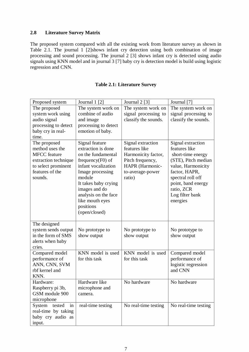
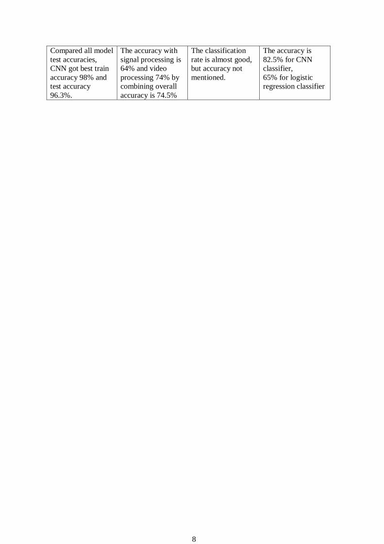
2.8 Literature Survey Matrix

The proposed system compared with all the existing work from literature survey as shown in

Table 2.1. The journal 1 [2]shows infant cry detection using both combination of image

processing and sound processing. The journal 2 [3] shows infant cry is detected using audio

signals using KNN model and in journal 3 [7] baby cry is detection model is build using logistic

regression and CNN.

Table 2.1: Literature Survey

Proposed system Journal 1 [2] Journal 2 [3] Journal [7]

The proposed

system work using

audio signal

processing to detect

baby cry in real-

time.

The system work on

combine of audio

and image

processing to detect

emotion of baby.

The system work on

signal processing to

classify the sounds.

The system work on

signal processing to

classify the sounds.

The proposed

method uses the

MFCC feature

extraction technique

to select prominent

features of the

sounds.

Signal feature

extraction is done

on the fundamental

frequency(F0) of

infant vocalization

Image processing

module

It takes baby crying

images and do

analysis on the face

like mouth eyes

positions

(open/closed)

Signal extraction

features like

Harmonicity factor,

Pitch frequency,

HAPR (Harmonic-

to-average-power

ratio)

Signal extraction

features like

short-time energy

(STE), Pitch median

value, Harmonicity

factor, HAPR,

spectral roll off

point, band energy

ratio, ZCR

Log filter bank

energies

The designed

system sends output

in the form of SMS

alerts when baby

cries.

No prototype to

show output

No prototype to

show output

No prototype to

show output

Compared model

performance of

ANN, CNN, SVM

rbf kernel and

KNN.

KNN model is used

for this task

KNN model is used

for this task

Compared model

performance of

logistic regression

and CNN

Hardware:

Raspberry pi 3b,

GSM module 900

microphone

Hardware like

microphone and

camera.

No hardware No hardware

System tested in

real-time by taking

baby cry audio as

input.

real-time testing No real-time testing No real-time testing

8

Compared all model

test accuracies,

CNN got best train

accuracy 98% and

test accuracy

96.3%.

The accuracy with

signal processing is

64% and video

processing 74% by

combining overall

accuracy is 74.5%

The classification

rate is almost good,

but accuracy not

mentioned.

The accuracy is

82.5% for CNN

classifier,

65% for logistic

regression classifier

9

CHAPTER 3

METHODOLOGY

3.1 System Overview

Key components of the system consist of Raspberry pi model 3B, USB (Universal serial Bus)

microphone, and output as GSM.

3.2 System Design

The methodology of the system development achieved in three stages.

Audio data collection of baby cry sounds and other domestic sounds.

Trained the data using SVM, KNN, ANN and CNN.

Deploy all trained algorithms in Raspberry pi for testing.

10

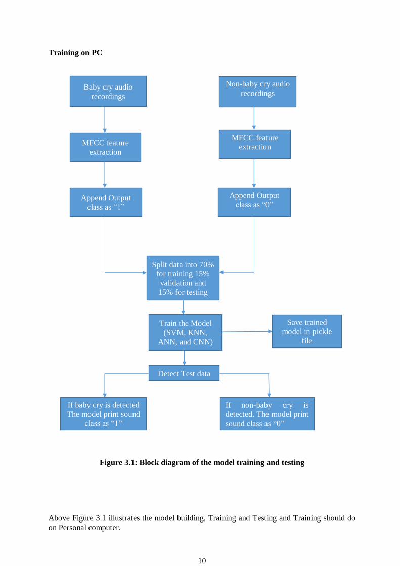
Training on PC

Figure 3.1: Block diagram of the model training and testing

Above Figure 3.1 illustrates the model building, Training and Testing and Training should do

on Personal computer.

Baby cry audio

recordings

Non-baby cry audio

recordings

MFCC feature

extraction

MFCC feature

extraction

Append Output

class as “1”

Append Output

class as “0”

Train the Model

(SVM, KNN,

ANN, and CNN)

Split data into 70%

for training 15%

validation and

15% for testing

Detect Test data

If baby cry is detected

The model print sound

class as “1”

If non-baby cry is

detected. The model print

sound class as “0”

Save trained

model in pickle

file

11

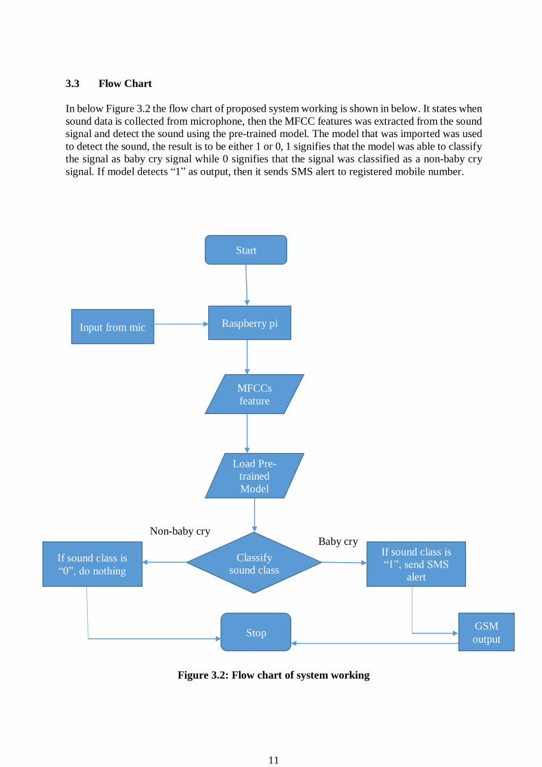
3.3 Flow Chart

In below Figure 3.2 the flow chart of proposed system working is shown in below. It states when

sound data is collected from microphone, then the MFCC features was extracted from the sound

signal and detect the sound using the pre-trained model. The model that was imported was used

to detect the sound, the result is to be either 1 or 0, 1 signifies that the model was able to classify

the signal as baby cry signal while 0 signifies that the signal was classified as a non-baby cry

signal. If model detects “1” as output, then it sends SMS alert to registered mobile number.

Figure 3.2: Flow chart of system working

Start

Raspberry pi Input from mic

MFCCs

feature

Load Pre-

trained

Model

Classify

sound class

class

If sound class is

“1”, send SMS

alert

Stop

If sound class is

“0”, do nothing

GSM

output

Baby cry Non-baby cry

12

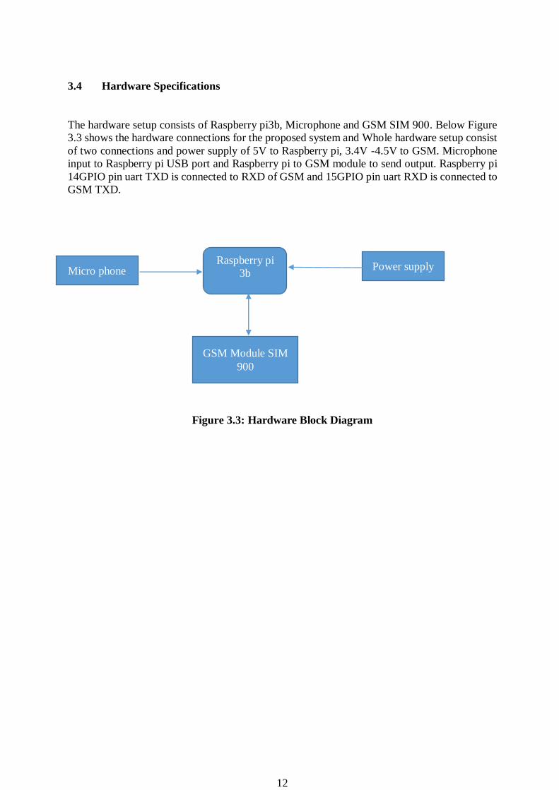
3.4 Hardware Specifications

The hardware setup consists of Raspberry pi3b, Microphone and GSM SIM 900. Below Figure

3.3 shows the hardware connections for the proposed system and Whole hardware setup consist

of two connections and power supply of 5V to Raspberry pi, 3.4V -4.5V to GSM. Microphone

input to Raspberry pi USB port and Raspberry pi to GSM module to send output. Raspberry pi

14GPIO pin uart TXD is connected to RXD of GSM and 15GPIO pin uart RXD is connected to

GSM TXD.

Figure 3.3: Hardware Block Diagram

GSM Module SIM

900

Micro phone Raspberry pi

3b

Power supply

13

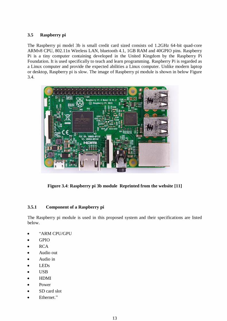
3.5 Raspberry pi

The Raspberry pi model 3b is small credit card sized consists od 1.2GHz 64-bit quad-core

ARMv8 CPU, 802.11n Wireless LAN, bluetooth 4.1, 1GB RAM and 40GPIO pins. Raspberry

Pi is a tiny computer containing developed in the United Kingdom by the Raspberry Pi

Foundation. It is used specifically to teach and learn programming. Raspberry Pi is regarded as

a Linux computer and provide the expected abilities a Linux computer. Unlike modern laptop

or desktop, Raspberry pi is slow. The image of Raspberry pi module is shown in below Figure

3.4.

Figure 3.4: Raspberry pi 3b module Reprinted from the website [11]

3.5.1 Component of a Raspberry pi

The Raspberry pi module is used in this proposed system and their specifications are listed

below.

“ARM CPU/GPU

GPIO

RCA

Audio out

Audio in

LEDs

USB

HDMI

Power

SD card slot

Ethernet.”

14

3.5.2 Setup up the Raspberry Pi

a) Hardware Setup

Power supply: A 5v power supply was provided

USB keyboard

USB Mouse

Micro SD USB card reader

Monitor

An Ethernet cable

Component of the set up

The setup of is made microphone, GSM module, power supply, and monitor.

b) Software Setup

Downloading operating system

The operating system was downloaded from Raspberrypi.com, NOOBs was

downloaded to computer

Formatting micro SD card

Copying the operating system file into the SD card

Slotting the SD card into Raspberry pi

Power on Raspberry pi

Waiting for installation process.

15

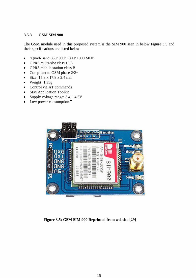
Figure 3.5: GSM SIM 900 Reprinted from website [29]

3.5.3 GSM SIM 900

The GSM module used in this proposed system is the SIM 900 seen in below Figure 3.5 and

their specifications are listed below

“Quad-Band 850/ 900/ 1800/ 1900 MHz

GPRS multi-slot class 10/8

GPRS mobile station class B

Compliant to GSM phase 2/2+

Size: 15.8 x 17.8 x 2.4 mm

Weight: 1.35g

Control via AT commands

SIM Application Toolkit

Supply voltage range: 3.4 ~ 4.3V

Low power consumption.”

16

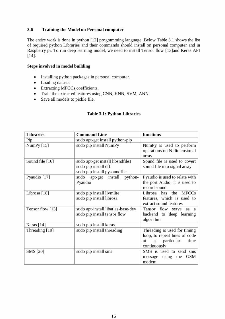
3.6 Training the Model on Personal computer

The entire work is done in python [12] programming language. Below Table 3.1 shows the list

of required python Libraries and their commands should install on personal computer and in

Raspberry pi. To run deep learning model, we need to install Tensor flow [13]and Keras API

[14].

Steps involved in model building

Installing python packages in personal computer.

Loading dataset

Extracting MFCCs coefficients.

Train the extracted features using CNN, KNN, SVM, ANN.

Save all models to pickle file.

Table 3.1: Python Libraries

Libraries Command Line functions

Pip sudo apt-get install python-pip

NumPy [15] sudo pip install NumPy NumPy is used to perform

operations on N dimensional

array

Sound file [16] sudo apt-get install libsndfile1

sudo pip install cffi

sudo pip install pysoundfile

Sound file is used to covert

sound file into signal array

Pyaudio [17] sudo apt-get install python-

Pyaudio

Pyaudio is used to relate with

the port Audio, it is used to

record sound

Librosa [18] sudo pip install llvmlite

sudo pip install librosa

Librosa has the MFCCs

features, which is used to

extract sound features

Tensor flow [13] sudo apt-install libatlas-base-dev

sudo pip install tensor flow

Tensor flow serve as a

backend to deep learning

algorithm

Keras [14] sudo pip install keras

Threading [19] sudo pip install threading Threading is used for timing

loop, to repeat lines of code

at a particular time

continuously

SMS [20] sudo pip install sms SMS is used to send sms

message using the GSM

modem

17

3.6.1 Model Building

The entire work is done on Jupiter notebook and with keras backend API [14]. Python functions

was written to produce the for mentioned features from the sounds, the file paths in the baby cry

array was used to extract the sound features by calling each of the functions. The first thing that

was done is importing the necessary modules.

3.6.2 Loading Dataset

Dataset of baby cry recordings and other sounds download from source [21] the data set consist

of baby cry, baby laugh, silences, noises and some traffic sounds of total length 1275 files [22].

The audio is in .ogg format which can be used for pre-processing. Extraction of sounds paths

into an array, the downloaded data was kept in different folders. The file paths were specified in

the python program. The sounds were classified into two arrays in the code which was the baby

cry array and the non-baby cry array. The baby cry array entails sound from the baby cry folder

while the non-baby cry array consists of sounds from the baby laugh, baby silence and noise.

And other domestic sounds. Module os was used to access the directory of the sounds file using

the attribute listdir. The directory of each folder (baby cry, baby laugh, silence and noise) was

defined as variables.

3.6.3 Mel-Frequency Cepstrum Coefficients (MFCCs)

Frame the signal into short frames.

For each frame calculate the periodogram estimate of the power spectrum.

Apply the Mel filter bank to the power spectra, sum the energy in each filter.

Take the logarithm of all filter bank energies.

Take the DCT of the log filter bank energies.

Keep DCT coefficients 2-13, discard the rest.

The entire process explained step by step to make MFCCs features.

An audio signal is constantly changing, so to simplify things we assume that on short time scales

the audio signal doesn't change. This is why we frame the signal into 20-40ms frames. If the

frame is much shorter, we don't have enough samples to get a reliable spectral estimate, if it is

longer the signal changes too much throughout the frame [23].

The next step is to calculate the power spectrum of each frame. This is motivated by the human

cochlea (an organ in the ear) which vibrates at different spots depending on the frequency of the

incoming sounds. periodogram helps to identify which frequencies are present in the frame. The

periodogram spectral estimate still contains a lot of information not required for Automatic

Speech Recognition (ASR), should take clumps of periodogram bins and sum them up to get an

idea of how much energy exists in various frequency regions. This is performed by Mel filter

bank; the first filter is very narrow and gives an indication of how much energy exists near 0

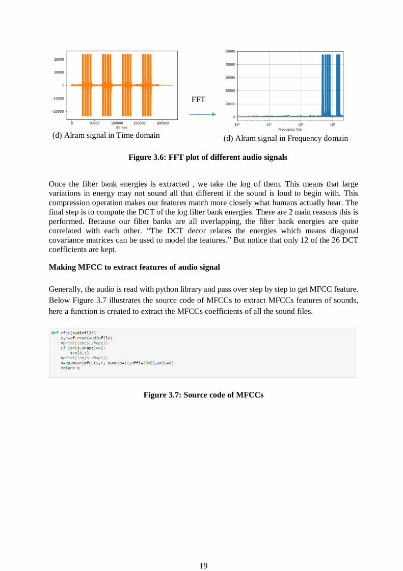
Hertz. Figure 3.6 shows power spectrum of audio signals taken in dataset (a) represents baby

cry, (b) represents baby Laugh, (c) represents baby silence, (d) represents alarm sound.

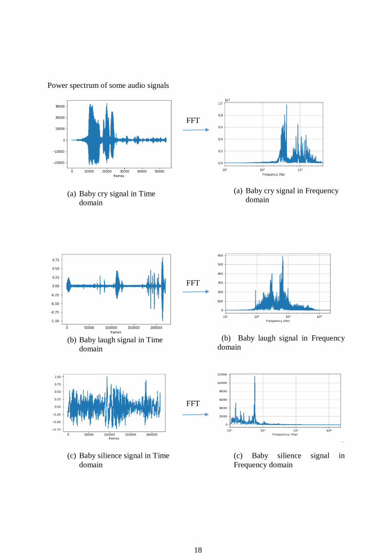
18

Power spectrum of some audio signals

(a) Baby cry signal in Time

domain

FFT

(a) Baby cry signal in Frequency

domain

(b) Baby laugh signal in Time

domain

FFT

(b) Baby laugh signal in Frequency

domain

(c) Baby silience signal in Time

domain

FFT

(c) Baby silience signal in

Frequency domain

19

(d) Alram signal in Time domain

FFT

(d) Alram signal in Frequency domain

Figure 3.6: FFT plot of different audio signals

Once the filter bank energies is extracted , we take the log of them. This means that large

variations in energy may not sound all that different if the sound is loud to begin with. This

compression operation makes our features match more closely what humans actually hear. The

final step is to compute the DCT of the log filter bank energies. There are 2 main reasons this is

performed. Because our filter banks are all overlapping, the filter bank energies are quite

correlated with each other. “The DCT decor relates the energies which means diagonal

covariance matrices can be used to model the features.” But notice that only 12 of the 26 DCT

coefficients are kept.

Making MFCC to extract features of audio signal

Generally, the audio is read with python library and pass over step by step to get MFCC feature.

Below Figure 3.7 illustrates the source code of MFCCs to extract MFCCs features of sounds,

here a function is created to extract the MFCCs coefficients of all the sound files.

Figure 3.7: Source code of MFCCs

20

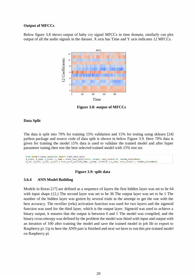
Output of MFCCs

Below figure 3.8 shows output of baby cry signal MFCCs in time domain, similarly can plot

output of all the audio signals in the dataset. X axis has Time and Y axis indicates 12 MFCCs.

Figure 3.8: output of MFCCs

Data Split

The data is split into 70% for training 15% validation and 15% for testing using sklearn [24]

python package and source code of data split is shown in below Figure 3.9. Here 70% data is

given for training the model 15% data is used to validate the trained model and after hyper

parameter tuning then test the best selected trained model with 15% test set.

3.6.4 ANN Model Building

Models in Keras [17] are defined as a sequence of layers the first hidden layer was set to be 64

with input shape (12,) The second layer was set to be 36 The output layer was set to be 1 The

number of the hidden layer was gotten by several trials in the attempt to get the one with the

best accuracy. The rectifier (relu) activation function was used for two layers and the sigmoid

function was used for the third layer, which is the output layer. Sigmoid was used to achieve a

binary output, it ensures that the output is between 0 and 1 The model was compiled, and the

binary cross entropy was defined by the problem the model was fitted with input and output with

an iteration of 100 after training the model and save the trained model in job lib to export to

Raspberry pi. Up to here the ANN part is finished and next we have to run this pre-trained model

on Raspberry pi.

Figure 3.9: split data

Time

1

2 C

oef

ficie

nts

21

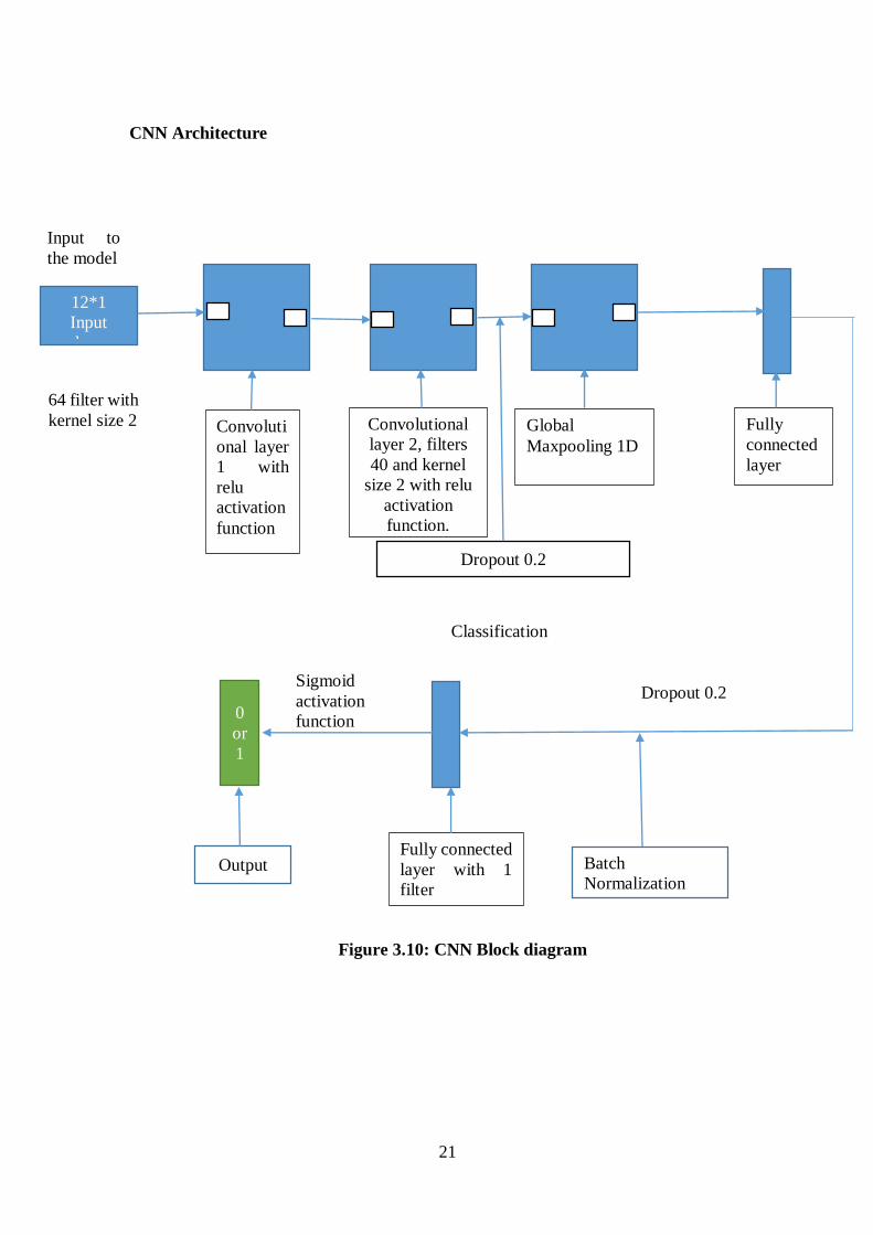
3.6.5 Proposed Convolutional Neural Networks

After extracting MFCC coefficients of size (1275, 12). The size is reshaped to (1275, 64, 12) to

have spatial dimensional to feed input to CNN. Below Figure 3.10 explains the proposed CNN

architecture model step by step in blocks. The CNN architecture consists of input layer, 2

convolutional layers + max pooling layer followed by two fully connected layers and output

layer. To specify the input shape first we passed sequential layer. Convolution is applied to input

data using a convolutional filter to produce a feature map. For conv1D layer the filter size is set

64 filters, kernel size set 2, input shape given (64, 12) with relu activation function. We perform

the convolution operation by sliding this filter over the input. At every location, we do element-

wise matrix multiplication and sum the result. This sum goes into the feature map. We again pass

the result of the convolution operation through relu activation function. So, the values in the final

feature maps are not actually the sums, but the relu function applied to them. The output of this

layer is given another convolutional layer with 40 filters and kernel size set to 2 with padding,

strides set to 1 and relu activation function is used. Padding is commonly used in CNN to

preserve the size of the feature maps. “The next hidden layer is Global max pooling layer which

helps effectively down sample the output of prior layer reducing the number of operations

required for all the following layer, but still passing on the valid information from the previous

layer.” In between layers we added dropout layer to avoid over fitting of the model it as a

regularization technique the dropout hyper parameter is set 0.2 after the convolution + pooling

layers we add a couple of fully connected layers to wrap up the CNN architecture. The next

hidden layer is dense layer 40 neurons for linear operation of previous layer. Batch

normalization layer is added in between two convolutional layers substitute of dropout layer.

“The use of Batch Normalization between the linear and non-linear layers in the network,

because it normalizes the input to your activation function”. One more dense layer is used as

hidden layer and finally we used sigmoid activation function in the output layer because the

model detects the output in form of 0 or 1.

21

CNN Architecture

12*1

Input

shape

0

or

1

Input to

the model

Convoluti

onal layer

1 with

relu

activation

function

Convolutional

layer 2, filters

40 and kernel

size 2 with relu

activation

function.

Global

Maxpooling 1D

64 filter with

kernel size 2 Fully

connected

layer

Dropout 0.2

Fully connected

layer with 1

filter

Sigmoid

activation

function

Output

Classification

Dropout 0.2

Batch

Normalization

Figure 3.10: CNN Block diagram

22

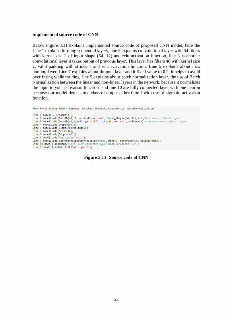
Implemented source code of CNN

Below Figure 3.11 explains implemented source code of proposed CNN model, here the

Line 1 explains forming sequential layers, line 2 explains convolutional layer with 64 filters

with kernel size 2 of input shape (64, 12) and relu activation function, line 3 is another

convolutional layer it takes output of previous layer. This layer has filters 40 with kernel size

2, valid padding with strides 1 and relu activation function. Line 5 explains about max

pooling layer. Line 7 explains about dropout layer and it fixed value to 0.2, it helps to avoid

over fitting while training. line 9 explains about batch normalization layer, the use of Batch

Normalization between the linear and non-linear layers in the network, because it normalizes

the input to your activation function and line 10 are fully connected layer with one neuron

because our model detects one class of output either 0 or 1 with use of sigmoid activation

function.

Figure 3.11: Source code of CNN

23

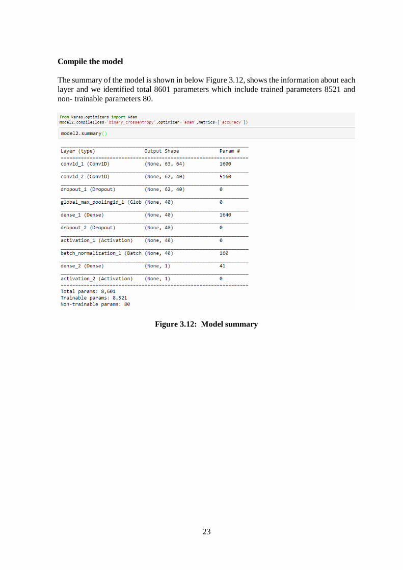
Compile the model

The summary of the model is shown in below Figure 3.12, shows the information about each

layer and we identified total 8601 parameters which include trained parameters 8521 and

non- trainable parameters 80.

Figure 3.12: Model summary

24

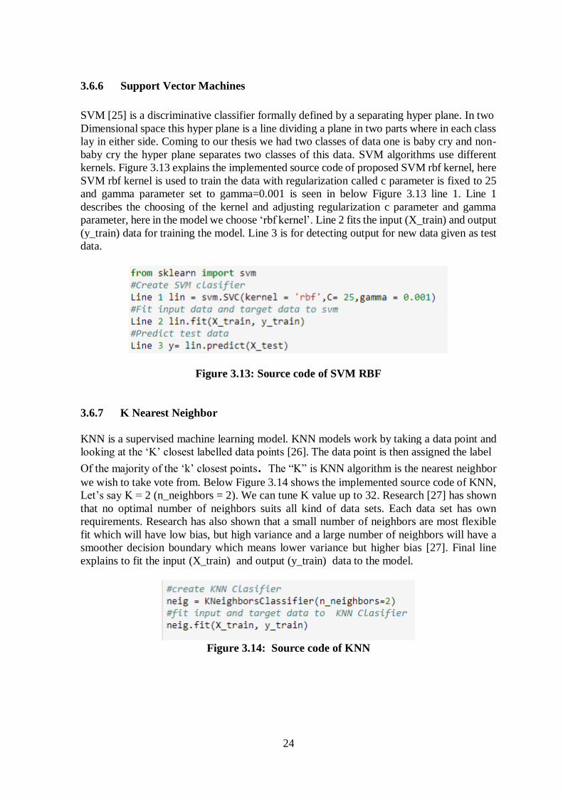
3.6.6 Support Vector Machines

SVM [25] is a discriminative classifier formally defined by a separating hyper plane. In two

Dimensional space this hyper plane is a line dividing a plane in two parts where in each class

lay in either side. Coming to our thesis we had two classes of data one is baby cry and non-

baby cry the hyper plane separates two classes of this data. SVM algorithms use different

kernels. Figure 3.13 explains the implemented source code of proposed SVM rbf kernel, here

SVM rbf kernel is used to train the data with regularization called c parameter is fixed to 25

and gamma parameter set to gamma=0.001 is seen in below Figure 3.13 line 1. Line 1

describes the choosing of the kernel and adjusting regularization c parameter and gamma

parameter, here in the model we choose ‘rbf kernel’. Line 2 fits the input (X_train) and output

(y_train) data for training the model. Line 3 is for detecting output for new data given as test

data.

Figure 3.13: Source code of SVM RBF

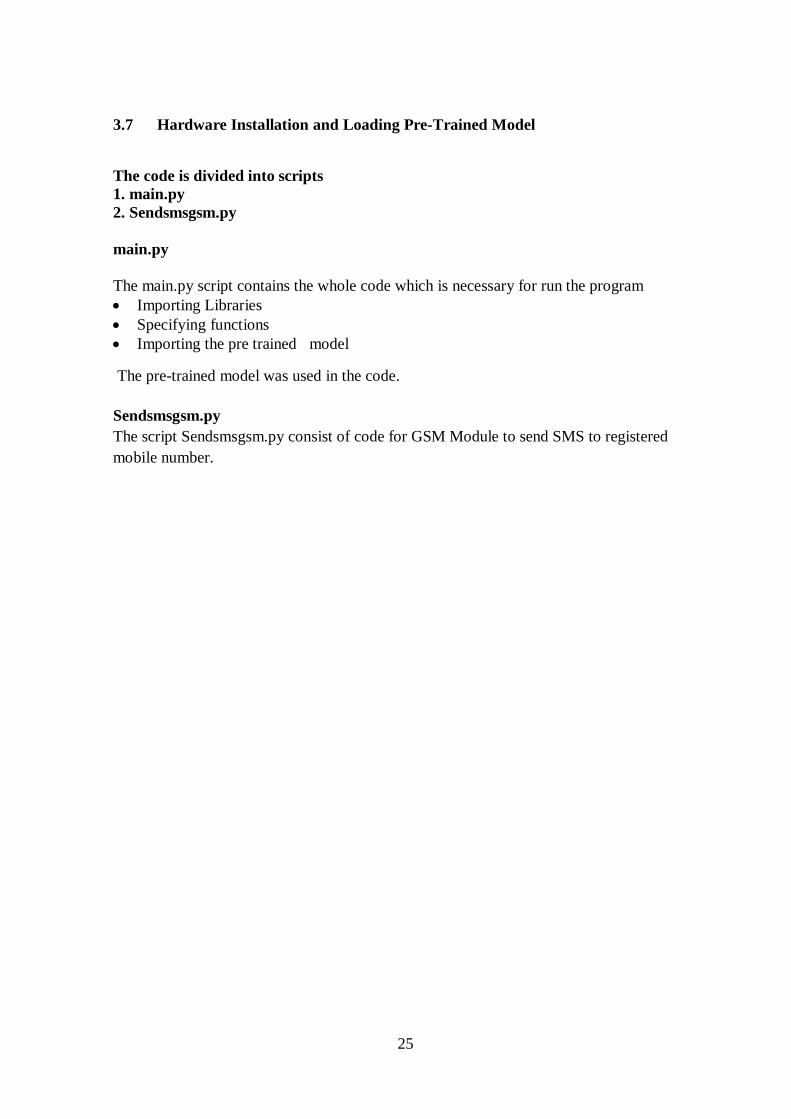
3.6.7 K Nearest Neighbor

KNN is a supervised machine learning model. KNN models work by taking a data point and

looking at the ‘K’ closest labelled data points [26]. The data point is then assigned the label

Of the majority of the ‘k’ closest points. The “K” is KNN algorithm is the nearest neighbor

we wish to take vote from. Below Figure 3.14 shows the implemented source code of KNN,

Let’s say K = 2 (n_neighbors = 2). We can tune K value up to 32. Research [27] has shown

that no optimal number of neighbors suits all kind of data sets. Each data set has own

requirements. Research has also shown that a small number of neighbors are most flexible

fit which will have low bias, but high variance and a large number of neighbors will have a

smoother decision boundary which means lower variance but higher bias [27]. Final line

explains to fit the input (X_train) and output (y_train) data to the model.

Figure 3.14: Source code of KNN

25

3.7 Hardware Installation and Loading Pre-Trained Model

The code is divided into scripts

1. main.py

2. Sendsmsgsm.py

main.py

The main.py script contains the whole code which is necessary for run the program

Importing Libraries

Specifying functions

Importing the pre trained model

The pre-trained model was used in the code.

Sendsmsgsm.py

The script Sendsmsgsm.py consist of code for GSM Module to send SMS to registered

mobile number.

26

3.8 Configuring Auto run

It is very important to auto-start all the programs upon booting-up of the Raspberry

pi. It is done using rc.local.

This was done with the steps below

Change boot from desktop to CLI

Editing profile configuration to setup program to run automatically when power

up the Raspberry pi.

Final setup after installation of the system

The final setup of Raspberry pi connected with USB microphone and GSM module. It is

placed near baby cradle with required power supply and when baby starts crying then the

model takes 5 seconds sound from the input microphone and detect sound with the help of

pre-trained model, if the model detects baby cry then system can send SMS alerts to

registered mobile number.

27

CHAPTER 4

EXPERIMENTAL RESULTS

4.1 Models

Data taken total 1275 sounds (718 baby cry, 557 non-baby cry) here 892 sounds are given

for training. 191 sounds are used to validate the trained model and finally after hyper

parameter tuning test best model with test set of 192 sounds.

Artificial Neural Network (ANN)

Convolutional Neural Network (CNN)

Support Vector Machine RBF kernel (SVM)

K Nearest Neighbor (KNN)

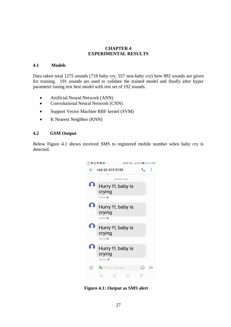
4.2 GSM Output

Below Figure 4.1 shows received SMS to registered mobile number when baby cry is

detected.

Figure 4.1: Output as SMS alert

28

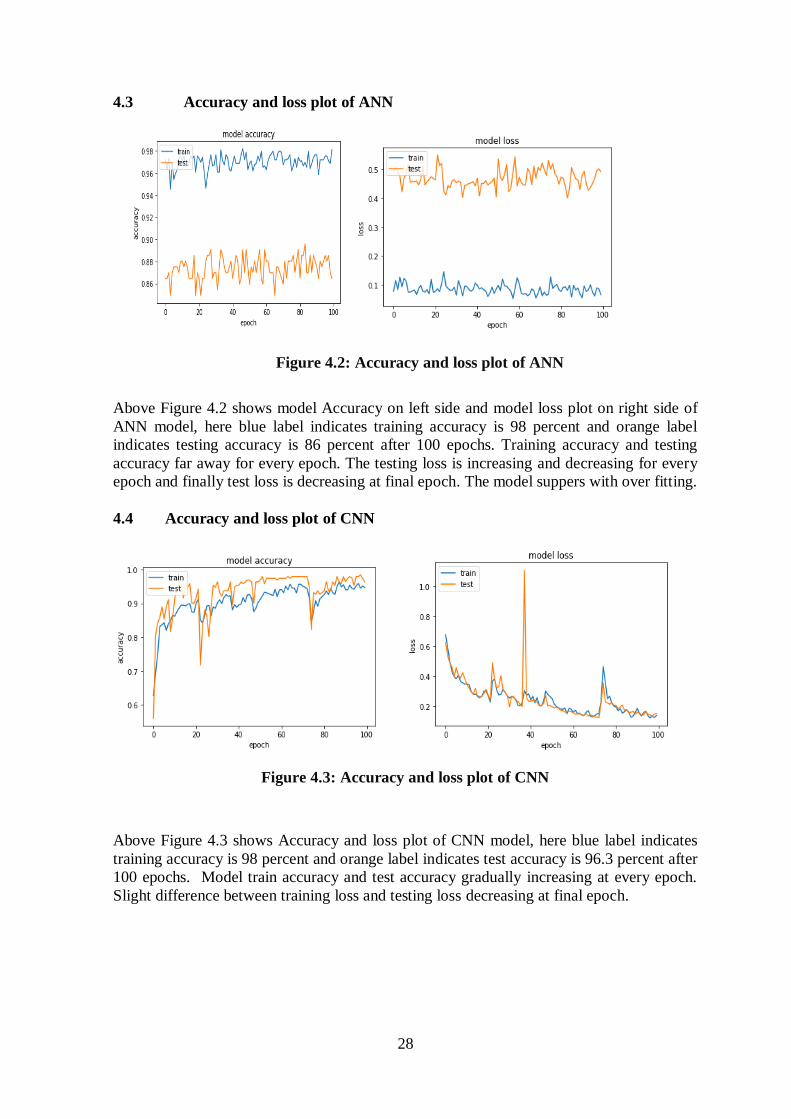
Figure 4.2: Accuracy and loss plot of ANN

4.3 Accuracy and loss plot of ANN

Above Figure 4.2 shows model Accuracy on left side and model loss plot on right side of

ANN model, here blue label indicates training accuracy is 98 percent and orange label

indicates testing accuracy is 86 percent after 100 epochs. Training accuracy and testing

accuracy far away for every epoch. The testing loss is increasing and decreasing for every

epoch and finally test loss is decreasing at final epoch. The model suppers with over fitting.

4.4 Accuracy and loss plot of CNN

Figure 4.3: Accuracy and loss plot of CNN

Above Figure 4.3 shows Accuracy and loss plot of CNN model, here blue label indicates

training accuracy is 98 percent and orange label indicates test accuracy is 96.3 percent after

100 epochs. Model train accuracy and test accuracy gradually increasing at every epoch.

Slight difference between training loss and testing loss decreasing at final epoch.

29

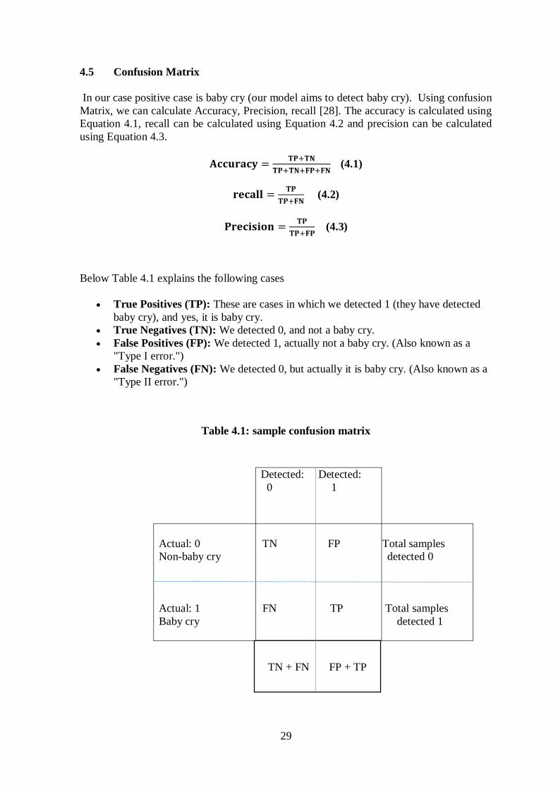
4.5 Confusion Matrix

In our case positive case is baby cry (our model aims to detect baby cry). Using confusion

Matrix, we can calculate Accuracy, Precision, recall [28]. The accuracy is calculated using

Equation 4.1, recall can be calculated using Equation 4.2 and precision can be calculated

using Equation 4.3.

𝐀𝐜𝐜𝐮𝐫𝐚𝐜𝐲 =𝐓𝐏+𝐓𝐍

𝐓𝐏+𝐓𝐍+𝐅𝐏+𝐅𝐍 (4.1)

𝐫𝐞𝐜𝐚𝐥𝐥 =𝐓𝐏

𝐓𝐏+𝐅𝐍 (4.2)

𝐏𝐫𝐞𝐜𝐢𝐬𝐢𝐨𝐧 =𝐓𝐏

𝐓𝐏+𝐅𝐏 (4.3)

Below Table 4.1 explains the following cases

True Positives (TP): These are cases in which we detected 1 (they have detected

baby cry), and yes, it is baby cry.

True Negatives (TN): We detected 0, and not a baby cry.

False Positives (FP): We detected 1, actually not a baby cry. (Also known as a

"Type I error.")

False Negatives (FN): We detected 0, but actually it is baby cry. (Also known as a

"Type II error.")

Table 4.1: sample confusion matrix

Detected: Detected:

0 1

Actual: 0 TN FP Total samples

Non-baby cry detected 0

Actual: 1 FN TP Total samples

Baby cry detected 1

STN + FN FP + TP

30

Figure 4.4: Confusion matrix of ANN

4.6 Confusion matrix of ANN

Above Figure 4.4 shows the Confusion matrix of ANN, here 0 represents non-baby cry and

1 represents baby cry. The model detects True positive 100 as baby cry and True Negative

66 as non-baby cry among 192 samples.

To calculate accuracy of the ANN model from Figure 4.4

𝐀𝐜𝐜𝐮𝐫𝐚𝐜𝐲 =𝐓𝐏+𝐓𝐍

𝐓𝐏+𝐓𝐍+𝐅𝐏+𝐅𝐍 (4.1)

Accuracy =100+66

100+66+10+16*100

Accuracy = 86%

TP = True Positive, TN = True Negative, FP = False Positive, FN = False Negative.

To calculate recall from Figure 4.4

𝐫𝐞𝐜𝐚𝐥𝐥 =𝐓𝐏

𝐓𝐏+𝐅𝐍 (4.2)

recall =100

100+16 *100

recall = 86%

31

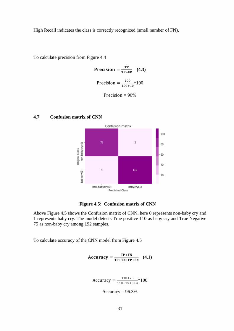
Figure 4.5: Confusion matrix of CNN

High Recall indicates the class is correctly recognized (small number of FN).

To calculate precision from Figure 4.4

𝐏𝐫𝐞𝐜𝐢𝐬𝐢𝐨𝐧 =𝐓𝐏

𝐓𝐏+𝐅𝐏 (4.3)

Precision =100

100+10*100

Precision = 90%

4.7 Confusion matrix of CNN

Above Figure 4.5 shows the Confusion matrix of CNN, here 0 represents non-baby cry and

1 represents baby cry. The model detects True positive 110 as baby cry and True Negative

75 as non-baby cry among 192 samples.

To calculate accuracy of the CNN model from Figure 4.5

𝐀𝐜𝐜𝐮𝐫𝐚𝐜𝐲 =𝐓𝐏+𝐓𝐍

𝐓𝐏+𝐓𝐍+𝐅𝐏+𝐅𝐍 (4.1)

Accuracy =110+75

110+75+3+4*100

Accuracy = 96.3%

32

TP = True Positive, TN = True Negative, FP = False Positive, FN = False Negative.

To calculate recall from Figure 4.5

𝐫𝐞𝐜𝐚𝐥𝐥 =𝐓𝐏

𝐓𝐏+𝐅𝐍 (4.2)

recall =110

110+4 *100

recall = 96.4%

High Recall indicates the class is correctly recognized (small number of FN).

To calculate precision from Figure 4.5

𝐏𝐫𝐞𝐜𝐢𝐬𝐢𝐨𝐧 =𝐓𝐏

𝐓𝐏+𝐅𝐏 (4.3)

Precision =110

110+3*100

Precision = 97.3%

33

4.8 Confusion matrix of SVM

Figure 4.6: Confusion matrix of SVM

Above Figure 4.6 shows the Confusion matrix of SVM. Here 0 represents non-baby cry and

1 represents baby cry. Model detects True Negative 79 as non-baby cry and True Positive

100 as baby cry among 192 samples.

To calculate accuracy of the SVM rbf from Figure 4.6

𝐀𝐜𝐜𝐮𝐫𝐚𝐜𝐲 =𝐓𝐏+𝐓𝐍

𝐓𝐏+𝐓𝐍+𝐅𝐏+𝐅𝐍 (4.1)

Accuracy =100+79

100+79+4+9*100

Accuracy = 93.2%

TP = True Positive, TN = True Negative, FP = False Positive, FN = False Negative.

To calculate recall from Figure 4.6

𝐫𝐞𝐜𝐚𝐥𝐥 =𝐓𝐏

𝐓𝐏+𝐅𝐍 (4.2)

recall =100

100+4 *100

34

recall = 96%

To calculate precision from Figure 4.6

𝐏𝐫𝐞𝐜𝐢𝐬𝐢𝐨𝐧 =𝐓𝐏

𝐓𝐏+𝐅𝐏 (4.3)

Precision =100

100+9*100

Precision = 92%

4.9 Confusion matrix of KNN

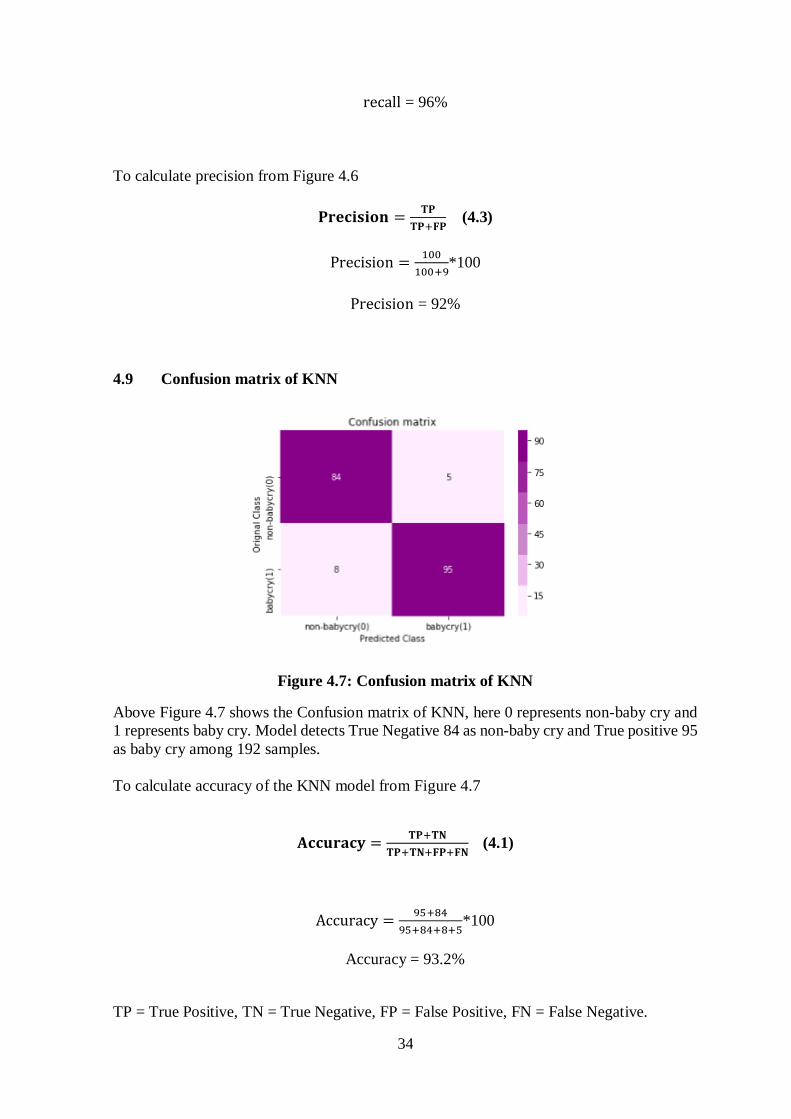
Figure 4.7: Confusion matrix of KNN Above Figure 4.7 shows the Confusion matrix of KNN, here 0 represents non-baby cry and

1 represents baby cry. Model detects True Negative 84 as non-baby cry and True positive 95

as baby cry among 192 samples.

To calculate accuracy of the KNN model from Figure 4.7

𝐀𝐜𝐜𝐮𝐫𝐚𝐜𝐲 =𝐓𝐏+𝐓𝐍

𝐓𝐏+𝐓𝐍+𝐅𝐏+𝐅𝐍 (4.1)

Accuracy =95+84

95+84+8+5*100

Accuracy = 93.2%

TP = True Positive, TN = True Negative, FP = False Positive, FN = False Negative.

35

To calculate recall from Figure 4.7

𝐫𝐞𝐜𝐚𝐥𝐥 =𝐓𝐏

𝐓𝐏+𝐅𝐍 (4.2)

recall =95

95+8 *100

recall = 92.2%

High Recall indicates the class is correctly recognized (small number of FN).

To calculate precision from Figure 4.7

𝐩𝐫𝐞𝐜𝐢𝐬𝐢𝐨𝐧 =𝐓𝐏

𝐓𝐏+𝐅𝐏 (4.3)

Precision =95

95+5*100

Precision = 95%

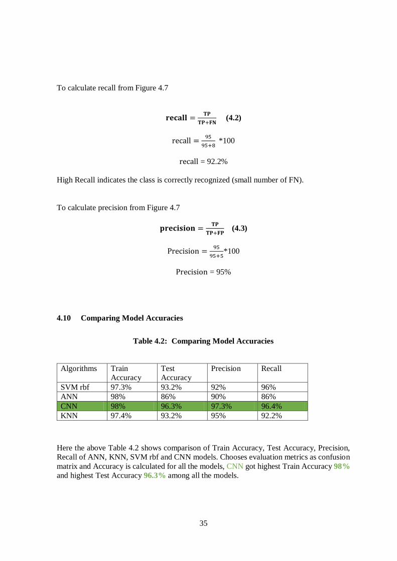
4.10 Comparing Model Accuracies

Table 4.2: Comparing Model Accuracies

Algorithms Train

Accuracy

Test

Accuracy

Precision Recall

SVM rbf 97.3% 93.2% 92% 96%

ANN 98% 86% 90% 86%

CNN 98% 96.3% 97.3% 96.4%

KNN 97.4% 93.2% 95% 92.2%

Here the above Table 4.2 shows comparison of Train Accuracy, Test Accuracy, Precision,

Recall of ANN, KNN, SVM rbf and CNN models. Chooses evaluation metrics as confusion

matrix and Accuracy is calculated for all the models, CNN got highest Train Accuracy 98%

and highest Test Accuracy 96.3% among all the models.

36

37

CHAPTER 5

CONCLUSION AND RECOMMENDATIONS

5.1 Conclusion

This thesis goal is to develop a system to detect baby cry. The goal is reached in proposed

three objectives. The goal of objective one is to train the data using SVM, KNN, ANN, and

CNN. The second goal is to load the pre-trained model in Raspberry pi for real-time testing

and final objective is to send SMS alert when cry is detected. The developed system detects

baby cry when baby starts crying and send SMS alerts to registered mobile number. Finally,

CNN model is loaded in Raspberry pi and the device is tested in real-time and it performed

well.

5.2 Recommendations

This system can be integrated in many ways to show output.

If the baby cries, we can set output to play a song. In this way the baby may stops

crying.

Can integrate too many applications related to baby care.

38

REFERENCES

[1] I. Suaste-Rivas, A. Díaz-Méndez, C. Reyes-García and O. Reyes-Galaviz, "Hybrid

Neural Network Design and Implementation on FPGA for Infant Cry Recognition," in

Text, Speech and Dialogue, Berlin, Heidelberg, Springer, 2006, pp. 703-709.

[2] P. Pal, A. Iyer and R. Yantorno, "Emotion Detection From Infant Facial Expressions

And Cries," in International Conference on Acoustics Speed and Signal Processing

Proceedings, 2006.

[3] Lavner, R. Cohen and Y., "Infant cry analysis and detection," Convention of Electrical

and Electronics Engineers in Israel, 2012.

[4] M. Hariharan, J. Saraswathy , R. Sindhu , Wan Khairunizam , Sazali Yaacob, "Infant

cry classification to identify asphyxia using time-frequency analysis," Expert Systems

with Applications, 2012.

[5] Y. K. Tadj, "Frequential Characterization of Healthy and Pathologic Newborns Cries,"

Article.sapub.org, 2013.

[6] Lu Wenping, H. W. L. Y and Li Min., "A facial expression recognition method for

baby video surveillance," in 3rd International Conference on Multimedia Technology

Proceeding, 2013.

[7] Yizhar Lavner, Rami Cohen, Dima Ruinskiy and Hans IJzerman, "Baby Cry Detection

in Domestic Environment using deep learning," ICSEE International Conference on

the Science of Electrical Engineering, 2016.

[8] Chen, Chuan-Yu ChangEmail authorChuan-Wang ChangS. KathiravanChen LinSzu-

Ta, "DAG-SVM based infant cry classification system using sequential forward

floating feature selection," Multidimensional Systems and Signal Processing, vol. 28,

no. 3, p. 961–976, 2016.

[9] A. C. N. Suwannata, "The Features Extraction of Infants Cries by Using Discrete

Wavelet Transform Techniques," 2016 International Electrical Engineering Congress,

iEECON2016, 2-4 March 2016, Chiang Mai, Thailand, 2016.

[10] Gaurav Naithani,Email author, Jaana Kivinummi, Tuomas Virtanen, Outi Tammela,

Mikko J. Peltola and Jukka M. Leppänen, "Automatic segmentation of infant cry

39

signals using hidden Markov models," EURASIP Journal on Audio, Speech, and

Music Processing, 26 January 2018.

[11] ""Raspberry Pi — Teach, Learn, and Make with Raspberry Pi"," R. Foundation, 2018.

[Online]. Available: https://www.raspberrypi.org.

[12] "Python.org," Welcome to Python.org, 2018. [Online]. Available:

https://www.python.org/..

[13] "TensorFlow," 2018. [Online]. Available: https://www.tensorflow.org/.

[14] "Guide to the Functional API - Keras Documentation, Keras.io," [Online]. Available:

https://keras.io/getting-started/functional-api-guide/.

[15] " Numpy.org," NumPy — NumPy, [Online]. Available: http://www.numpy.org/.

[16] "pysound," 2018. [Online]. Available: https://pypi.org/project/pysound/. [Accessed

2018].

[17] "PyAudio Documentation — PyAudio 0.2.11 documentation," People.csail.mit.edu,

2018. [Online]. Available: https://people.csail.mit.edu/hubert/pyaudio/docs/.

[Accessed 2018].

[18] "librosa.feature.mfcc — librosa 0.6.2 documentation", Librosa.github.io, 2018,"

librosa, [Online]. Available:

https://librosa.github.io/librosa/generated/librosa.feature.mfcc.html.

[19] " Docs.python.org," threading — Thread-based parallelism — Python 3.7.2rc1

documentation, [Online]. Available: https://docs.python.org/3/library/threading.html.

[20] "sms-api," PyPI, 2018. [Online]. Available: Available: https://pypi.org/project/sms-

api/. [Accessed 2018].

[21] K. J. Piczak, "ESC: Dataset for Environmental Sound Classification," in Proceedings

of the 23rd Annual ACM Conference on Multimedia, Brisbane, Australia, 2015.

[22] "Github," [Online]. Available: https://github.com/gveres/donateacry-corpus.

40

[23] jameslyons. [Online]. Available:

http://practicalcryptography.com/miscellaneous/machine-learning/guide-mel-

frequency-cepstral-coefficients-mfccs/.

[24] Pedregosa, F. and Varoquaux, G. and Gramfort, A. and Michel, "Scikit-learn: Machine

Learning in {P}ython," Journal of Machine Learning Research, vol. 12, pp. 2825--

2830, 2011.

[25] Kone Chaka, Nhan Le-Thanh, Remi Flamary and Cecile Belleudy, "Performance

Comparison of the KNN and SVM Classification Algorithms in the Emotion Detection

System EMOTICA," International Journal of Sensor Networks and Data

Communications, vol. 7, 2018.

[26] E. Allibhai, "Towards Data Science," sep 2018. [Online]. Available:

https://towardsdatascience.com/building-a-k-nearest-neighbors-k-nn-model-with-

scikit-learn-51209555453a.

[27] A. Navlani, "KNN Classification using Scikit-learn," DataCamp, aug 2018. [Online].

Available: https://www.datacamp.com/community/tutorials/k-nearest-neighbor-

classification-scikit-learn.

[28] W. Koehrsen, "Towards Data Science," 3 March 2018. [Online]. Available:

https://towardsdatascience.com/beyond-accuracy-precision-and-recall-3da06bea9f6c.

[29] "Simcom.ee," SIM900 | SIMCom | smart machines, smart decision | simcom.ee, , 2018.

[Online]. Available: https://simcom.ee/modules/gsm-gprs/sim900/.