Embed Size (px)
Citation preview

NEW MEXICO DEPARTMENT OF TRANSPORTATION
RREESSEEAARRCCHH BBUURREEAAUU
Innovation in Transportation
Development and Validation of a Unified Equation for Drilled Shaft Foundation Design in New Mexico
Prepared by: University of New Mexico Albuquerque, NM 87131 Prepared for: New Mexico Department of Transportation Research Bureau 7500B Pan American Freeway NE Albuquerque, NM 87109 In Cooperation with: The US Department of Transportation Federal Highway Administration
Report NM10MSC-01 December 3, 2012

SUMMARY PAGE
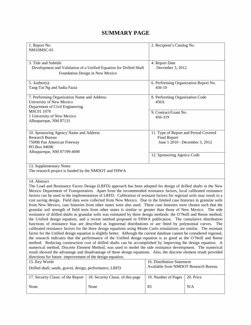
1. Report No. NM10MSC-01
2. Recipient’s Catalog No.
3. Title and Subtitle Development and Validation of a Unified Equation for Drilled Shaft
Foundation Design in New Mexico
4. Report Date December 3, 2012
5. Author(s): Tang-Tat Ng and Sadia Fazia
6. Performing Organization Report No. 456-10
7. Performing Organization Name and Address University of New Mexico Department of Civil Engineering MSC01 1070 1 University of New Mexico Albuquerque, NM 87131
8. Performing Organization Code 456A
9. Contract/Grant No. 456-319
10. Sponsoring Agency Name and Address Research Bureau 7500B Pan American Freeway PO Box 94690 Albuquerque, NM 87199-4690
11. Type of Report and Period Covered Final Report June 1 2010 - December 3, 2012
12. Sponsoring Agency Code
13. Supplementary Notes The research project is funded by the NMDOT and FHWA 14. Abstract The Load and Resistance Factor Design (LRFD) approach has been adopted for design of drilled shafts in the New Mexico Department of Transportation. Apart from the recommended resistance factors, local calibrated resistance factors can be used in the implementation of LRFD. Calibration of resistant factors for regional soils may result in a cost saving design. Field data were collected from New Mexico. Due to the limited case histories in granular soils from New Mexico, case histories from other states were also used. These case histories were chosen such that the granular soil strength of field tests from other states is similar or greater than those of New Mexico. The side resistance of drilled shafts in granular soils was estimated by three design methods: the O’Neill and Reese method, the Unified design equation, and a recent method proposed in FHWA publication. The cumulative distribution functions of resistance bias are described as lognormal distributions or are fitted by polynomial curves. The calibrated resistance factors for the three design equations using Monte Carlo simulations are similar. The resistant factor for the Unified design equation is slightly better. Although the current database cannot be considered regional, the research indicates that the performance of the Unified design equation is as good as the O’Neill and Reese method. Reducing construction cost of drilled shafts can be accomplished by improving the design equation. A numerical method, Discrete Element Method, was used to model the side resistance development. The numerical result showed the advantage and disadvantage of these design equations. Also, the discrete element result provided directions for future improvement of the design equation. 15. Key Words 16. Distribution Statement
Available from NMDOT Research Bureau Drilled shaft, sands, gravel, design, performance, LRFD
17. Security Classi. of the Report None
18. Security Classi. of this page None
19. Number of Pages 83
20. Price N/A

Project No. NM10MSC-01
Development and Validation of a Unified Equation for Drilled Shaft
Foundation Design in New Mexico
Final Report
By
Tang-Tat Ng, Ph.D., P.E. Sadia Faiza, Graduate Research Assistant
Department of Civil Engineering MSC01 1070, Albuquerque, N.M. 87131
University of New Mexico
Report NM10MSC-01
A Report on Research Sponsored by New Mexico Department of Transportation
Research Bureau
in Cooperation with The U.S. Department of Transportation
Federal Highway Administration December 2012
NMDOT Research Bureau 7500B Pan American Freeway NE
PO Box 94690 Albuquerque, NM 87199-4690
(505) 841-9145
© New Mexico Department of Transportation
i
PREFACE
The research reported herein collects the case studies of field testing of drilled shaft in sands. This project conducts an in-depth literature search, and establishes contacts with state Departments of Transportation.
NOTICE
The United States government and the State of New Mexico do not endorse products or manufacturers. Trade or manufactures’ names appear herein solely because they are considered essential to the object of this report. This information is available in alternative accessible formats. To obtain an alternative format, contact the NMDOT Research Bureau, 7500B Pan American Freeway NE, PO Box 94690, Albuquerque, NM 87199-4690, (505)-841-9145
DISCLAIMER
This report presents the results of research conducted by the authors and does not necessarily reflect the views of the New Mexico Department of Transportation. This report does not constitute a standard or specification.
ii
EXECUTIVE SUMMARY
The Load and Resistance Factor Design (LRFD) approach has been adopted for design of drilled shafts by the New Mexico Department of Transportation. Although resistance factors have been recommended nationally, soil conditions and construction methods are different regionally. Calibration of the resistant factor for regional soils may result in a cost saving design. Field data of drilled shaft load tests in granular soils were collected from New Mexico and other states since there are only a few load tests conducted in New Mexico. We selected the field tests from other states such that the soil strength is similar or greater than the soil strength of New Mexico. The side resistance factor of drilled shafts in granular materials was calibrated for three design equations. They are the O’Neill and Reese method, the Unified Design equation, and the design method proposed in a recent FHWA publication. For the O’Neill and Reese method, the calibrated resistance factor by assuming the resistance bias is lognormal distribution is similar to the calibrated resistant factors reported by other researchers. When the cumulative distributed function of resistance bias is fitted by polynomial curves, the calibrated resistance factors for these three design equations are similar. The resistant factor for the Unified Design equation is slightly better. The result indicates that the performance of the Unified design equation is as good as the O’Neill and Reese method for this non-regional database. Reducing construction cost of drilled shafts can also be accomplished by improving the design equation. Numerical simulations using the Discrete Element Method have been carried out to model the development of side resistance. The numerical result has shown that the relationship between the side resistance and void ratio (relative density) is quite complicated. The side resistance is a function of relative density, vertical stress, and overconsolidation ratio (OCR). For normally consolidated samples at a certain confining pressure, a simple hyperbolic curve can be used to describe the relationship between the nominal side resistance and void ratio. The effect of OCR on side resistance is rather intricate. More numerical data are needed to identify the role of OCR.
The DEM simulations have indicated the advantages and disadvantages of the design equations. All design equations capture some of the nonlinear effect of depth on side resistance. The OCR term in the original Unified design equation is important. The effect of depth on side resistance is more complex than the simple function in the design equations. The DEM simulations indicated that the effect of OCR on side resistance is different from that of the design method proposed in a recent FHWA publication.
This research implies that a better design equation can be developed based on DEM simulations. However, current DEM simulations are limited such that a design equation cannot be defined completely. More DEM simulations are needed to clearly identify and describe the trend of certain factors. The DEM result can be used to modify and improve the Unified design equation. A small COV of the resistance bias can be obtained for a better Unified design equation. Then, a higher resistance factor will be calibrated from the reliability analysis.

iii
ACKNOWLEDGMENTS
This research is financially sponsored by the New Mexico Department of Transportation (NMDOT). The authors would like to thank the research Bureau Chief, Mr. Scott McClure for his support, and Administrator, Ms. Dee Billingsley for her fine accounting and reimbursements. The authors would like to thank the project technical panel for their helpful suggestions. The authors also would like to express their gratitude to Mr. James Wilson of ADOT who provided several case histories for this study. The authors appreciate the valuable service and time of Mr. Virgil Valdez, who is the project manager, and Mr. Bob Meyers, who is the sponsor of this project. Special thanks go Ms. Rebekah Lucero, UNM Civil Engineering accountant.
iv
Table of Contents
Introduction ..........................................................................................................................1
Background ..........................................................................................................................3
Drilled Shafts .................................................................................................................3
Design Resistance of Drilled Shafts ..............................................................................3
Prediction of Side Resistance of Drilled Shafts .............................................................4
The O’Neill and Reese Method (O’Neill and Reese 1999) ...........................................5
The NHI Method (FHWA 2010) ...................................................................................6
The Unified Design Equation (Chua et al. 2000) ..........................................................7
LRFD Calibration Using Reliability Theory .................................................................8
Monte Carlo Method ....................................................................................................11
Methodology ......................................................................................................................12
Database Collection and Evaluation ............................................................................12
LRFD Results.....................................................................................................................15
Statistical Analysis .......................................................................................................15
Calibration of Resistance Factor (Monte Carlo Method) ............................................20
The Discrete Element Analysis ..........................................................................................21
Side Resistance Simulations ........................................................................................24
Overconsolidated Samples ...........................................................................................29
Conclusions and Implementation Plan...............................................................................31
Implementation Plan ....................................................................................................31
References ..........................................................................................................................33
Appendix. ...........................................................................................................................37
v
LIST OF TABLES
TABLE 1 Final selected Cases. .................................................................................................... 13
TABLE 2 Statistics of the Bias of the Three Design Methods. .................................................... 15
TABLE 3 Statistics of the Bias of the Best-Fit-to-Tail Distributions. .......................................... 18
TABLE 4 Shaft Information ......................................................................................................... 37
TABLE 5 Soil Profile ................................................................................................................... 37
TABLE 6 Strain gage locations .................................................................................................... 37
TABLE 7 Shaft Information ........................................................................................................ 38
TABLE 8 Soil Profile ................................................................................................................... 38
TABLE 9 Strain Gage locations ................................................................................................... 39
TABLE 10 Shaft Information ....................................................................................................... 40
TABLE 11 Soil Profile ................................................................................................................. 40
TABLE 12 Shaft Information ....................................................................................................... 41
TABLE 13 Soil Profile ................................................................................................................. 41
TABLE 14 Shaft Information ....................................................................................................... 42
TABLE 15 Soil Profile ................................................................................................................. 42
TABLE 16 Strain Gage locations ................................................................................................. 42
TABLE 17 Shaft Information ....................................................................................................... 43
TABLE 18 Soil Profile ................................................................................................................. 43
TABLE 19 Shaft Information ....................................................................................................... 44
TABLE 20 Soil Profile ................................................................................................................. 44
TABLE 21 Shaft Information ....................................................................................................... 45
TABLE 22 Soil Profile ................................................................................................................. 45
TABLE 23 Strain Gage locations ................................................................................................. 46
TABLE 24 Shaft Information ....................................................................................................... 46
TABLE 25 Soil Profile ................................................................................................................. 47
TABLE 26 Strain Gage locations ................................................................................................. 47

vi
TABLE 27 Shaft Information ....................................................................................................... 49
TABLE 28 Soil Profile ................................................................................................................. 49
TABLE 29 Strain Gage locations ................................................................................................. 49
TABLE 30 Shaft Information ....................................................................................................... 51
TABLE 31 Soil Profile ................................................................................................................. 51
TABLE 32 Strain Gage locations ................................................................................................. 52
TABLE 33 Shaft Information ....................................................................................................... 53
TABLE 34 Soil Profile ................................................................................................................. 53
TABLE 35 Strain Gage Locations. ............................................................................................... 53
TABLE 36 Shaft Information ....................................................................................................... 55
TABLE 37 Soil Profile ................................................................................................................. 55
TABLE 38 Strain Gage locations ................................................................................................. 55
TABLE 39 Shaft Information ....................................................................................................... 56
TABLE 40 Soil Profile ................................................................................................................. 56
TABLE 41 Strain Gage locations ................................................................................................. 57
TABLE 42 Shaft Information ....................................................................................................... 58
TABLE 43 Soil Profile ................................................................................................................. 58
TABLE 44 Strain Gage locations ................................................................................................. 58
TABLE 45 Shaft Information ....................................................................................................... 60
TABLE 46 Soil Profile ................................................................................................................. 60
TABLE 47 Strain Gage locations ................................................................................................. 60
TABLE 48 Shaft Information ....................................................................................................... 61
TABLE 49 Soil Profile ................................................................................................................. 61
TABLE 50 Strain Gage locations ................................................................................................. 62
TABLE 51 Shaft Information ....................................................................................................... 63
TABLE 52 Soil Profile ................................................................................................................. 63
TABLE 53 Shaft Information ....................................................................................................... 64

vii
TABLE 54 Soil Profile ................................................................................................................. 64
TABLE 55 Shaft Information ....................................................................................................... 66
TABLE 56 Soil Profile ................................................................................................................. 66
TABLE 57 Shaft Information ....................................................................................................... 67
TABLE 58 Soil Profile ................................................................................................................. 67
TABLE 59 Shaft Information ....................................................................................................... 68
TABLE 60 Soil Profile ................................................................................................................. 68

viii
LIST OF FIGURES
FIGURE 1 Side Resistance and End Bearing of a Drilled Shaft. ................................................... 4
FIGURE 2 Side Resistance of Drilled Shaft. .................................................................................. 4
FIGURE 3 Angle of Internal Friction According to Soil Classification. ....................................... 8
FIGURE 4 Probability of Failure and Reliability Index (Withiam et al. 1998). ............................ 8
FIGURE 5 Relationship between ß and Pf. .................................................................................. 10
FIGURE 6 Measured vs. Predicted Side Resistance by the O’Neill & Reese Method. ............... 15
FIGURE 7 Measured vs. Predicted Side Resistance by the Unified Design Method. .................. 16
FIGURE 8 Measured vs. Predicted Side Resistance by the NHI Method. ................................... 16
FIGURE 9 CDF Plot of the Bias of Side Resistance Predicted by the O’Neill & Reese Method.17
FIGURE 10 CDF Plot of the Bias of Side Resistance Predicted by the Unified Design Method. 17
FIGURE 11 CDF Plot of the Bias of Side Resistance Predicted by the NHI Method. ................ 18
FIGURE 12 CDF Plot of the Bias for the Best Fit Polynomial Distribution. ............................... 19
FIGURE 13 A Numerical System used to simulate the Mobilization of Side Resistance. .......... 22
FIGURE 14 Behavior of Ko for Normally Consolidated Soil. ..................................................... 23
FIGURE 15 Behavior of Ko for Over-Consolidated Soil. ............................................................ 23
FIGURE 16 Behavior of the Ratio (Ko)OC/Ko. ............................................................................ 24
FIGURE 17 Result of Normally Consolidated Soil. ..................................................................... 25
FIGURE 18 The Dependence of ß on Initial Vertical Stresses and Void Ratio. .......................... 26
FIGURE 19 Comparison between the Hyperbolic Curve Fitting and Observed Data. ................ 27
FIGURE 20 Behavior of β with the Predicted Equations. ............................................................ 28
FIGURE 21 The Dependence of ß with Depth. ............................................................................ 29
FIGURE 22 Result of Overconsolidated Samples (σ = 2000 psf). ............................................... 30
FIGURE 23 Result of Overconsolidated Samples (OCR = 2). ..................................................... 30
FIGURE 24 Load Settlement Curve. ............................................................................................ 38
FIGURE 25 Load Settlement Curve. ............................................................................................ 39
ix
FIGURE 26 Load Settlement Curve. ............................................................................................ 40
FIGURE 27 Load Settlement Curve. ............................................................................................ 41
FIGURE 28 Load Settlement Curve. ............................................................................................ 43
FIGURE 29 Load Settlement Curve. ............................................................................................ 44
FIGURE 30 Load Settlement Curve. ............................................................................................ 45
FIGURE 31 Load Settlement Curve. ............................................................................................ 46
FIGURE 32 Load Settlement Curve. ............................................................................................ 47
FIGURE 33 Load Settlement Curve. ............................................................................................ 48
FIGURE 34 Load Settlement Curve. ............................................................................................ 48
FIGURE 35 Load Settlement Curve. ............................................................................................ 50
FIGURE 36 Load Settlement Curve. ............................................................................................ 50
FIGURE 37 Load Settlement Curve. ............................................................................................ 51
FIGURE 38 Load Settlement Curve. ............................................................................................ 52
FIGURE 39 Load Settlement Curve. ............................................................................................ 54
FIGURE 40 Load Settlement Curve. ............................................................................................ 56
FIGURE 41 Load Settlement Curve. ............................................................................................ 57
FIGURE 42 Load Settlement Curve. ............................................................................................ 59
FIGURE 43 Load Settlement Curve. ............................................................................................ 59
FIGURE 44 Load Settlement Curve. ............................................................................................ 61
FIGURE 45 Load Settlement Curve. ............................................................................................ 62
FIGURE 46 Load Settlement Curve. ............................................................................................ 63
FIGURE 47 Load Settlement Curve. ............................................................................................ 64
FIGURE 48 Load Settlement Curve. ............................................................................................ 66
FIGURE 49 Load Settlement Curve. ............................................................................................ 67
FIGURE 50 Load Settlement Curve. ............................................................................................ 68
1
Introduction
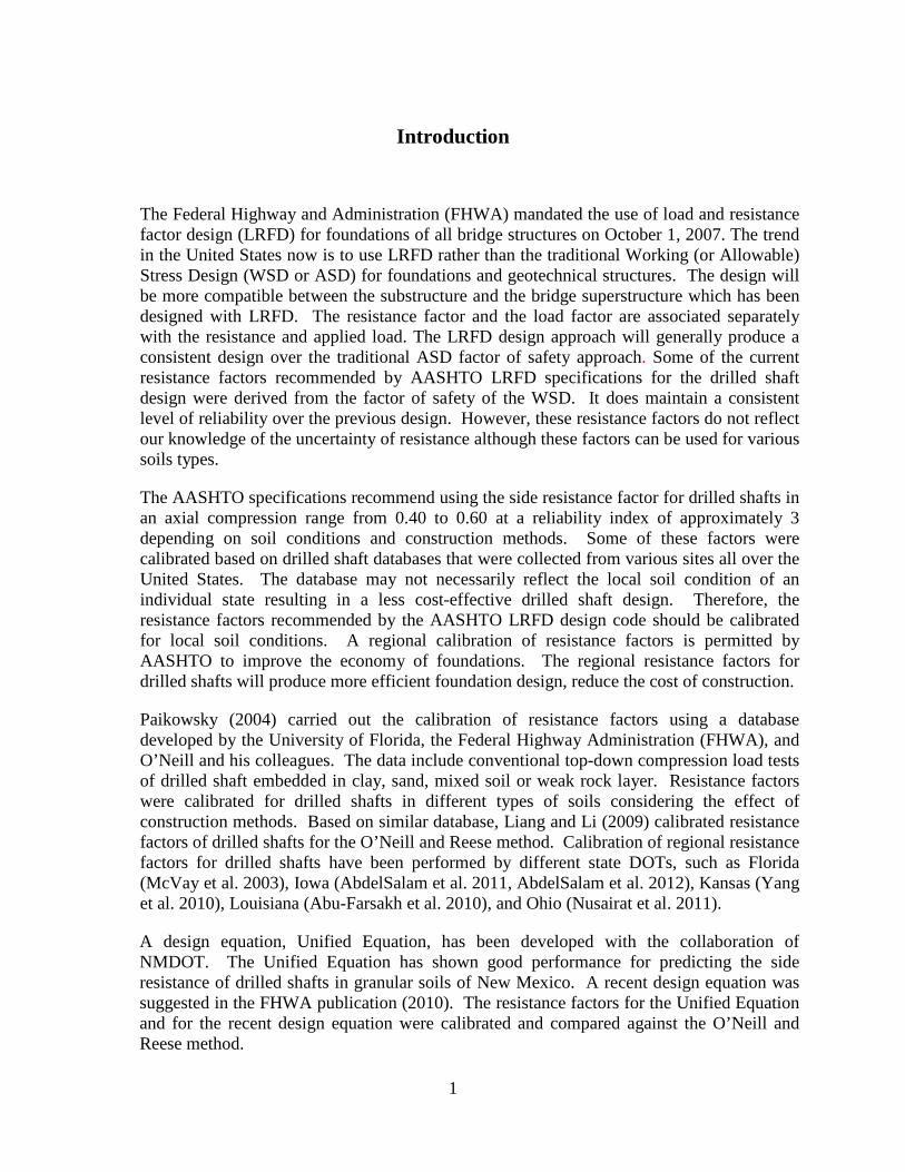
The Federal Highway and Administration (FHWA) mandated the use of load and resistance factor design (LRFD) for foundations of all bridge structures on October 1, 2007. The trend in the United States now is to use LRFD rather than the traditional Working (or Allowable) Stress Design (WSD or ASD) for foundations and geotechnical structures. The design will be more compatible between the substructure and the bridge superstructure which has been designed with LRFD. The resistance factor and the load factor are associated separately with the resistance and applied load. The LRFD design approach will generally produce a consistent design over the traditional ASD factor of safety approach. Some of the current resistance factors recommended by AASHTO LRFD specifications for the drilled shaft design were derived from the factor of safety of the WSD. It does maintain a consistent level of reliability over the previous design. However, these resistance factors do not reflect our knowledge of the uncertainty of resistance although these factors can be used for various soils types.
The AASHTO specifications recommend using the side resistance factor for drilled shafts in an axial compression range from 0.40 to 0.60 at a reliability index of approximately 3 depending on soil conditions and construction methods. Some of these factors were calibrated based on drilled shaft databases that were collected from various sites all over the United States. The database may not necessarily reflect the local soil condition of an individual state resulting in a less cost-effective drilled shaft design. Therefore, the resistance factors recommended by the AASHTO LRFD design code should be calibrated for local soil conditions. A regional calibration of resistance factors is permitted by AASHTO to improve the economy of foundations. The regional resistance factors for drilled shafts will produce more efficient foundation design, reduce the cost of construction.
Paikowsky (2004) carried out the calibration of resistance factors using a database developed by the University of Florida, the Federal Highway Administration (FHWA), and O’Neill and his colleagues. The data include conventional top-down compression load tests of drilled shaft embedded in clay, sand, mixed soil or weak rock layer. Resistance factors were calibrated for drilled shafts in different types of soils considering the effect of construction methods. Based on similar database, Liang and Li (2009) calibrated resistance factors of drilled shafts for the O’Neill and Reese method. Calibration of regional resistance factors for drilled shafts have been performed by different state DOTs, such as Florida (McVay et al. 2003), Iowa (AbdelSalam et al. 2011, AbdelSalam et al. 2012), Kansas (Yang et al. 2010), Louisiana (Abu-Farsakh et al. 2010), and Ohio (Nusairat et al. 2011).
A design equation, Unified Equation, has been developed with the collaboration of NMDOT. The Unified Equation has shown good performance for predicting the side resistance of drilled shafts in granular soils of New Mexico. A recent design equation was suggested in the FHWA publication (2010). The resistance factors for the Unified Equation and for the recent design equation were calibrated and compared against the O’Neill and Reese method.

2
Reducing construction cost of drilled shafts can be accomplished by improving the design equation. The numerical method, Discrete Element Method (DEM), was used to model the development of side resistance. The DEM result was compared against these design equations.
3
Background
Drilled Shafts
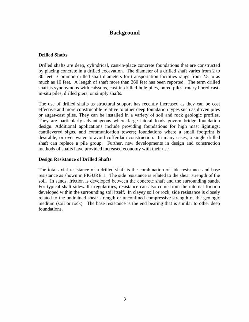
Drilled shafts are deep, cylindrical, cast-in-place concrete foundations that are constructed by placing concrete in a drilled excavation. The diameter of a drilled shaft varies from 2 to 30 feet. Common drilled shaft diameters for transportation facilities range from 2.5 to as much as 10 feet. A length of shaft more than 260 feet has been reported. The term drilled shaft is synonymous with caissons, cast-in-drilled-hole piles, bored piles, rotary bored cast-in-situ piles, drilled piers, or simply shafts.
The use of drilled shafts as structural support has recently increased as they can be cost effective and more constructible relative to other deep foundation types such as driven piles or auger-cast piles. They can be installed in a variety of soil and rock geologic profiles. They are particularly advantageous where large lateral loads govern bridge foundation design. Additional applications include providing foundations for high mast lightings; cantilevered signs, and communication towers; foundations where a small footprint is desirable; or over water to avoid cofferdam construction. In many cases, a single drilled shaft can replace a pile group. Further, new developments in design and construction methods of shafts have provided increased economy with their use.
Design Resistance of Drilled Shafts
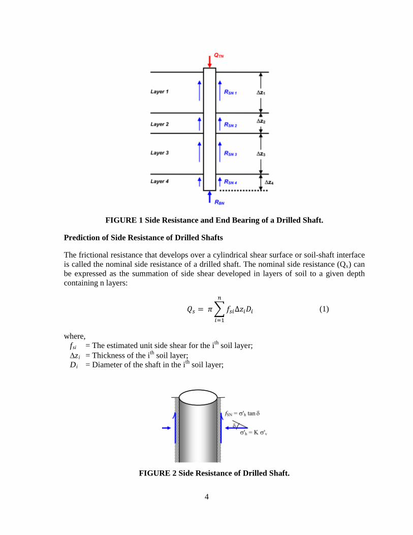
The total axial resistance of a drilled shaft is the combination of side resistance and base resistance as shown in FIGURE 1. The side resistance is related to the shear strength of the soil. In sands, friction is developed between the concrete shaft and the surrounding sands. For typical shaft sidewall irregularities, resistance can also come from the internal friction developed within the surrounding soil itself. In clayey soil or rock, side resistance is closely related to the undrained shear strength or unconfined compressive strength of the geologic medium (soil or rock). The base resistance is the end bearing that is similar to other deep foundations.
4
FIGURE 1 Side Resistance and End Bearing of a Drilled Shaft.
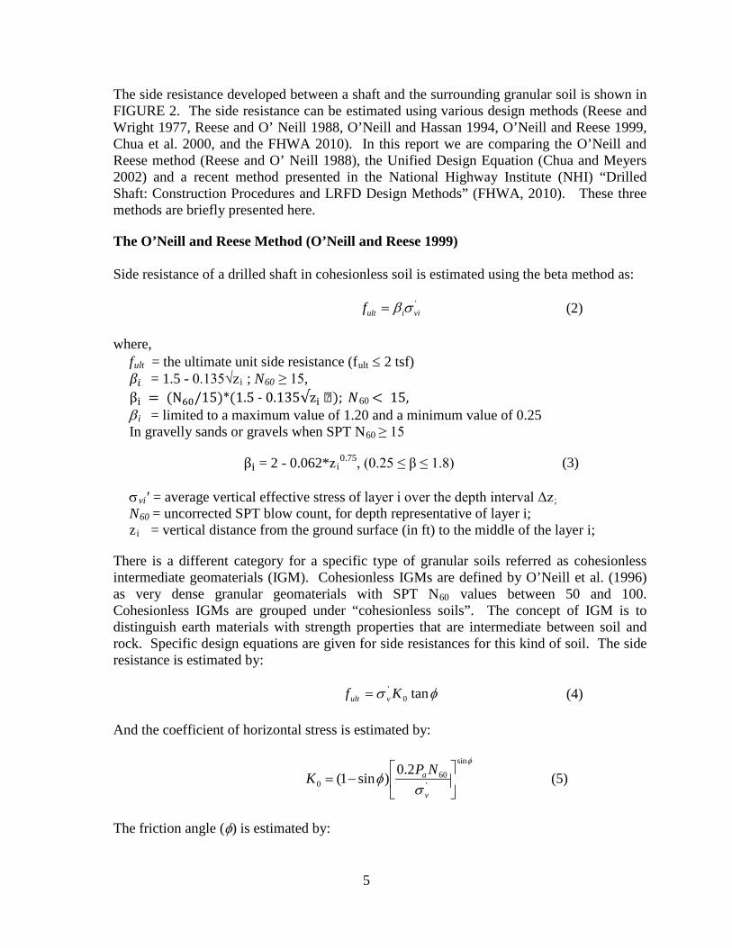
Prediction of Side Resistance of Drilled Shafts
The frictional resistance that develops over a cylindrical shear surface or soil-shaft interface is called the nominal side resistance of a drilled shaft. The nominal side resistance (Qs) can be expressed as the summation of side shear developed in layers of soil to a given depth containing n layers:
𝑄𝑠 = 𝜋�𝑓𝑠𝑖∆𝑧𝑖𝐷𝑖
𝑛
𝑖=1
(1)
where,
fsi = The estimated unit side shear for the ith soil layer; ∆zi = Thickness of the ith soil layer; Di = Diameter of the shaft in the ith soil layer;
FIGURE 2 Side Resistance of Drilled Shaft.
5
The side resistance developed between a shaft and the surrounding granular soil is shown in FIGURE 2. The side resistance can be estimated using various design methods (Reese and Wright 1977, Reese and O’ Neill 1988, O’Neill and Hassan 1994, O’Neill and Reese 1999, Chua et al. 2000, and the FHWA 2010). In this report we are comparing the O’Neill and Reese method (Reese and O’ Neill 1988), the Unified Design Equation (Chua and Meyers 2002) and a recent method presented in the National Highway Institute (NHI) “Drilled Shaft: Construction Procedures and LRFD Design Methods” (FHWA, 2010). These three methods are briefly presented here.
The O’Neill and Reese Method (O’Neill and Reese 1999)
Side resistance of a drilled shaft in cohesionless soil is estimated using the beta method as:
'viiultf σβ= (2)
where,
fult = the ultimate unit side resistance (fult ≤ 2 tsf) 𝛽𝑖 = 1.5 - 0.135√z i ; N60 ≥ 15, βi = (N60/15)*(1.5 - 0.135√zi �); 𝑁R60 < 15, βi = limited to a maximum value of 1.20 and a minimum value of 0.25 In gravelly sands or gravels when SPT N60 ≥ 15
βi = 2 - 0.062*zi0.75, (0.25 ≤ β ≤ 1.8) (3)
σvi′ = average vertical effective stress of layer i over the depth interval Δz ; N60 = uncorrected SPT blow count, for depth representative of layer i; zi = vertical distance from the ground surface (in ft) to the middle of the layer i;
There is a different category for a specific type of granular soils referred as cohesionless intermediate geomaterials (IGM). Cohesionless IGMs are defined by O’Neill et al. (1996) as very dense granular geomaterials with SPT N60 values between 50 and 100. Cohesionless IGMs are grouped under “cohesionless soils”. The concept of IGM is to distinguish earth materials with strength properties that are intermediate between soil and rock. Specific design equations are given for side resistances for this kind of soil. The side resistance is estimated by:
φσ tan0' Kf vult = (4)
And the coefficient of horizontal stress is estimated by:
φ
σφ
sin
'60
02.0)sin1(
−=
v
a NPK
(5)
The friction angle (φ) is estimated by:
6
34.0
'601
)(3.203.12tan
+= −
a
v
P
Nσ
φ
(6)
where, Pa = atmospheric pressure (1tsf).
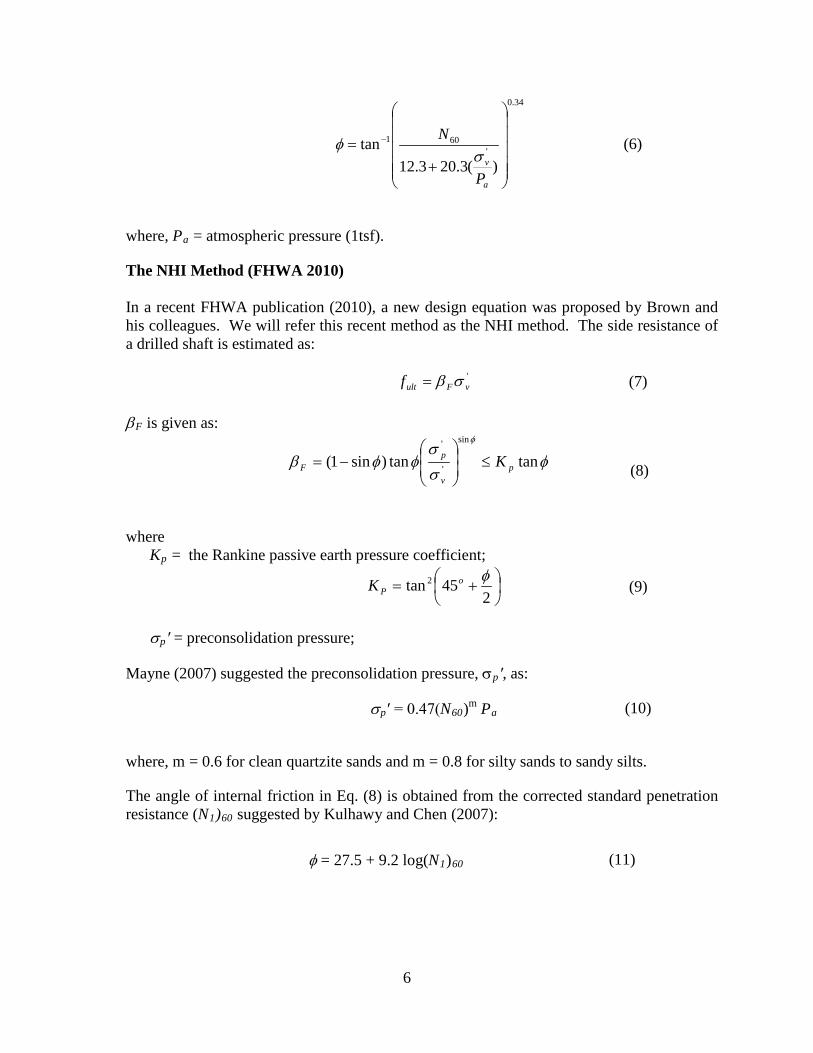
The NHI Method (FHWA 2010)
In a recent FHWA publication (2010), a new design equation was proposed by Brown and his colleagues. We will refer this recent method as the NHI method. The side resistance of a drilled shaft is estimated as:
'vFultf σβ= (7)
βF is given as:
φσσ
φφβφ
tantan)sin1(sin
'
'
pv
pF K≤
−=
(8)
where
Kp = the Rankine passive earth pressure coefficient;
+=
245tan 2 φo
PK (9)
σp′ = preconsolidation pressure;
Mayne (2007) suggested the preconsolidation pressure, σp′, as:
σp′ = 0.47(N60)m Pa (10)
where, m = 0.6 for clean quartzite sands and m = 0.8 for silty sands to sandy silts.
The angle of internal friction in Eq. (8) is obtained from the corrected standard penetration resistance (N1)60 suggested by Kulhawy and Chen (2007):
φ = 27.5 + 9.2 log(N1)60 (11)

7
The Unified Design Equation (Chua et al. 2000)
Chua et al. (2000) proposed a design equation for predicting the load-carrying capacity of drilled shafts in both cohesive and cohesionless soil. For a drilled shaft in cohesionless soils, the soil parameter needed for the design equation is the angle of internal friction as well as the unit weight of soils. This design equation has shown reasonable predictions for drilled shafts in granular soils of New Mexico.
In the Unified design equation (Chu and Meyers 2002), the βu value is calculated as:
+
−+−=
zKK
o
P
U 1
11tan)sin1( φφβ (12)
The nominal shaft resistance at depth z is:
'vuultf σβ= (13)
Gibbs and Holtz (1957) presented data that relate SPT blow counts to the relative density at different depths for sands. Chua et al. (2000) provided a predictive equation for the relative density based on regression analysis. The relative density (DR) is given as:
41.0223.0'
4.20 NP
Da
vR
−
=
σ (14)
Chua et al. (2000) also proposed a general equation between relative density and friction angle based on the data from Duncan et al (1980). The friction angle (φ) can be estimated as:
RD15.030 +=φ (15)
DM-7 (US Navy 1971) provides a correlation between friction angle and void ratio (relative density) for granular soils of different soil classifications. The relationships between the angle of international friction and DR for cohesionless soil are plotted in FIGURE 3.

8
FIGURE 3 Angle of Internal Friction According to Soil Classification.
Although Eq. 15 and FIGURE 3 give the estimation of friction angles, FIGURE 3 will be used here since it considers soil classification.
LRFD Calibration Using Reliability Theory
The basic concept behind LRFD calibration using reliability theory is illustrated in FIGURE 4. The distributions of random load (Q) and resistance (R) values are shown as normal distributions. The reliability based design treats load Q and resistance R components as random variables and targets the designed system to a particular probability of failure. The limit state function ‘g’ is the deviation of R and Q.
FIGURE 4 Probability of Failure and Reliability Index (Withiam et al. 1998).
The objective of LRFD is to ensure that for each limit state, the available resistance can be greater than the total load or somewhat less than the total load within acceptable risk.
2527293133353739414345
0 20 40 60 80 100
Ang
le o
f int
erna
l res
ista
nce
Relative density of granular soil
GW
GP
SW
SP
SM
ML
9
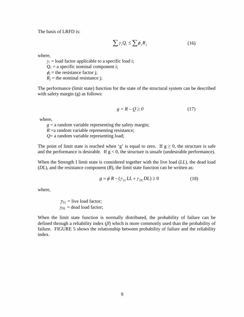
The basis of LRFD is:
jjii RQ ∑∑ ≤ φγ (16)
where,
γi = load factor applicable to a specific load i; Qi = a specific nominal component i; φj = the resistance factor j; Rj = the nominal resistance j;
The performance (limit state) function for the state of the structural system can be described with safety margin (g) as follows:
g = R – Q ≥ 0 (17)
where, g = a random variable representing the safety margin; R =a random variable representing resistance; Q= a random variable representing load;
The point of limit state is reached when ‘g’ is equal to zero. If g ≥ 0, the structure is safe and the performance is desirable. If g < 0, the structure is unsafe (undesirable performance).
When the Strength I limit state is considered together with the live load (LL), the dead load (DL), and the resistance component (R), the limit state function can be written as:
0)( ≥+−= DLLLRg DLLL γγφ (18)
where,
γLL = live load factor; γDL = dead load factor;
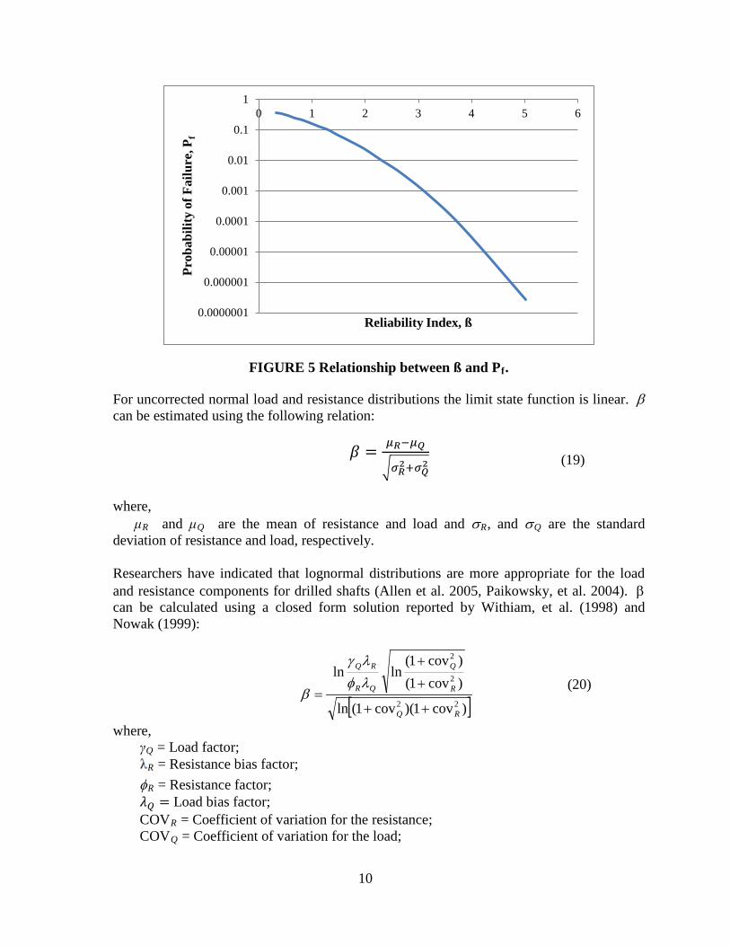
When the limit state function is normally distributed, the probability of failure can be defined through a reliability index (β) which is more commonly used than the probability of failure. FIGURE 5 shows the relationship between probability of failure and the reliability index.
10
FIGURE 5 Relationship between ß and Pf.
For uncorrected normal load and resistance distributions the limit state function is linear. β can be estimated using the following relation:
𝛽 = 𝜇𝑅−𝜇𝑄
�𝜎𝑅2+𝜎𝑄
2 (19)
where,
μR and μQ are the mean of resistance and load and σR, and σQ are the standard deviation of resistance and load, respectively.
Researchers have indicated that lognormal distributions are more appropriate for the load and resistance components for drilled shafts (Allen et al. 2005, Paikowsky, et al. 2004). β can be calculated using a closed form solution reported by Withiam, et al. (1998) and Nowak (1999):
[ ])cov1)(cov1(ln
)cov1()cov1(
lnln
22
2
2
RQ
R
Q
QR
RQ
++
+
+
=λφλγ
β (20)
where, γQ = Load factor;
R = Resistance bias factor; φR = Resistance factor; 𝜆𝑄 = Load bias factor; COVR = Coefficient of variation for the resistance; COVQ = Coefficient of variation for the load;
0.0000001
0.000001
0.00001
0.0001
0.001
0.01
0.1
10 1 2 3 4 5 6
Prob
abili
ty o
f Fai
lure
, Pf
Reliability Index, ß

11
When the lognormally distributed live and dead loads are considered, the resistance factor is estimated as:
[ ]( ))cov1)(covcov1(lnexp
)cov1()covcov1(ln
222
2
22
RLLDLLLLL
DLDL
R
LLDLLL
LL
DLDLR
R
++
+
++
+
=βλ
λ
γγ
λφ (21)
Where,
λDL = Dead load bias factor; COVDL = Coefficient of variation for the dead load; λLL = Live load bias factor; and
COVLL = Coefficient of variation for the live load;
When closed form solutions are unavailable, the Monte Carlo method is commonly used to calibrate the resistance factor (Allen et al. 2005).
Monte Carlo Method
The Monte Carlo method is a technique that utilizes a random number generator to generate values of random variables based on their own probability functions. The reliability index β is estimated from these values of random variables and the state function. Thus the probability of failure and reliability index can be estimated. The limit state function indicates that failure occurs at the point when the applied loads are just equal to or greater than the available resistance (g ≤ 0).
g = R - Q (22)
The steps of the Monte Carlo method used in this study are: I. Select a trial resistance factor (φ). Generate random numbers for each set of variables
(resistance, dead load and live load). Three random variables are generated independently. The limit state function, g, is then calculated for each pair of resistance and load (dead load and live load).
II. Determine the number of cases where g < 0. The probability of failure is the number of the failed cases (g < 0) divided by the total number of the cases generated:
50000
0<= gf
NP (23)
If the probability of failure is different from the desired value (0.001 in this study), another trial resistance factor (φ) will be used in step 1. The process is repeated until the desired probability of failure is obtained.

12
Methodology
Database Collection and Evaluation
To achieve the objectives of this study, ninety-five drilled shaft case histories of different lengths and diameters have been collected. The drilled shafts were tested either using the Osterberg cell (O-cell) method or conventional top-down static load test. The collected field test data were from NMDOT and from different parts of United States. The shafts are mostly in cohesionless soils.
An extensive search was conducted to collect all available drilled shaft case histories in New Mexico. Only five drilled shaft test cases in cohesionless soils of New Mexico are available. Due to the limited number of available cases in New Mexico, meaningful reliability analysis of drilled shaft cannot be accomplished. The accuracy of the results of a reliability analysis is directly dependent on the adequacy, in terms of quantity and quality, of the input data used. Therefore, drilled shaft cases in granular soils from different parts of the United States were also considered. Cases were selected such that the strength of the granular soils in other states is similar or stronger than those of the soils in New Mexico based on standard penetration resistance. Since the data are from different geographical regions, this research cannot be considered as a regional calibration. However, the determination of resistance factor for the Unified design equation in granular soils will be very helpful. In addition, the comparison among various design equations can be very useful to NMDOT geotechnical engineers.
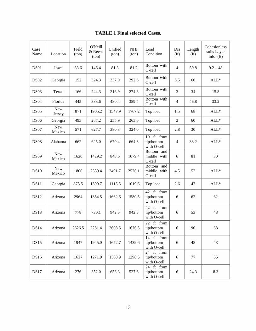
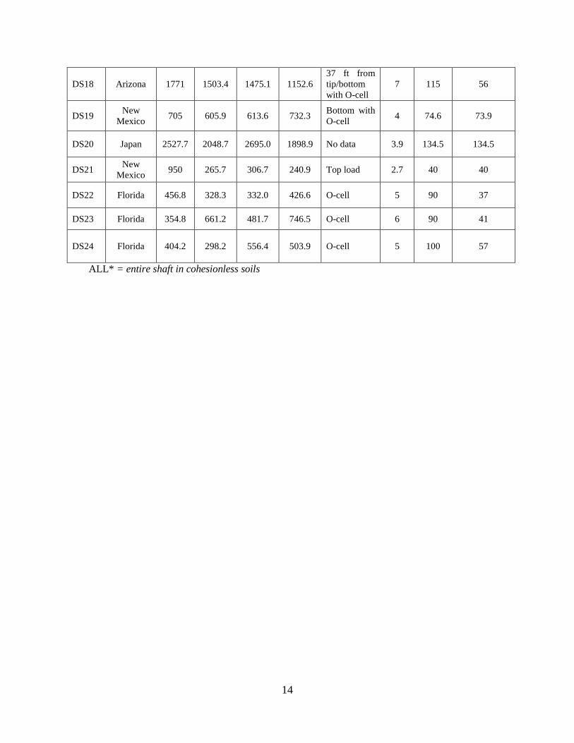
Finally, twenty-four drilled shaft case histories were selected and are reported. TABLE 1 shows the measured side resistance in the field, the side resistances estimated by the three design equations, the field loading condition (traditional top load or Osterberg cell ‘O-cell’), the diameter and length of the shaft, and the information of the cohesionless soils layers. Details of these cases can be found in the appendix.
The side resistances were determined in two ways; (a) the O-cell load-displacement curve was used to derive the total side resistance; and (b) the total side resistance is derived from the unit side resistance in each sub region from the strain gage data. The predicted values of side resistance were calculated by using the O’Neill and Reese’s method, the Unified design equation, and the NHI design method.
13
TABLE 1 Final selected Cases.
Case Name
Location
Field (ton)
O'Neill & Reese
(ton)
Unified (ton)
NHI (ton)
Load Condition
Dia (ft)
Length (ft)
Cohesionless soils Layer Info. (ft)
DS01 Iowa 83.6 146.4 81.3 81.2 Bottom with O-cell 4 59.8 9.2 – 48
DS02 Georgia 152 324.3 337.0 292.6 Bottom with O-cell 5.5 60 ALL*
DS03 Texas 166 244.3 216.9 274.8 Bottom with O-cell 3 34 15.8
DS04 Florida 445 383.6 480.4 389.4 Bottom with O-cell 4 46.8 33.2
DS05 New Jersey 871 1905.2 1547.9 1767.2 Top load 1.5 68 ALL*
DS06 Georgia 493 287.2 255.9 263.6 Top load 3 60 ALL*
DS07 New Mexico 571 627.7 380.3 324.0 Top load 2.8 30 ALL*
DS08 Alabama 662 625.0 670.4 664.3 10 ft from tip/bottom with O-cell
4 33.2 ALL*
DS09 New Mexico 1620 1429.2 848.6 1079.4
Bottom and middle with O-cell
6 81 30
DS10 New Mexico 1800 2559.4 2491.7 2526.1
Bottom and middle with O-cell
4.5 52 ALL*
DS11 Georgia 873.5 1399.7 1115.5 1019.6 Top load 2.6 47 ALL*
DS12 Arizona 2964 1354.5 1662.6 1580.5 42 ft from tip/bottom with O-cell
6 62
62
DS13 Arizona 778 730.1 942.5 942.5 42 ft from tip/bottom with O-cell
6 53 48
DS14 Arizona 2626.5 2281.4 2608.5 1676.3 22 ft from tip/bottom with O-cell
6 90 68
DS15 Arizona 1947 1945.0 1672.7 1439.6 14 ft from tip/bottom with O-cell
6 48 48
DS16 Arizona 1627 1271.9 1308.9 1298.5 24 ft from tip/bottom with O-cell
6 77 55
DS17 Arizona 276 352.0 653.3 527.6 24 ft from tip/bottom with O-cell
6 24.3 8.3
14
DS18 Arizona 1771 1503.4 1475.1 1152.6 37 ft from tip/bottom with O-cell
7 115 56
DS19 New Mexico 705 605.9 613.6 732.3 Bottom with
O-cell 4 74.6 73.9
DS20 Japan 2527.7 2048.7 2695.0 1898.9 No data 3.9 134.5 134.5
DS21 New Mexico 950 265.7 306.7 240.9 Top load 2.7 40 40
DS22 Florida 456.8 328.3 332.0 426.6 O-cell 5 90 37
DS23 Florida 354.8 661.2 481.7 746.5 O-cell 6 90 41
DS24 Florida 404.2 298.2 556.4 503.9 O-cell 5 100
57
ALL* = entire shaft in cohesionless soils
15
LRFD Results
Statistical Analysis
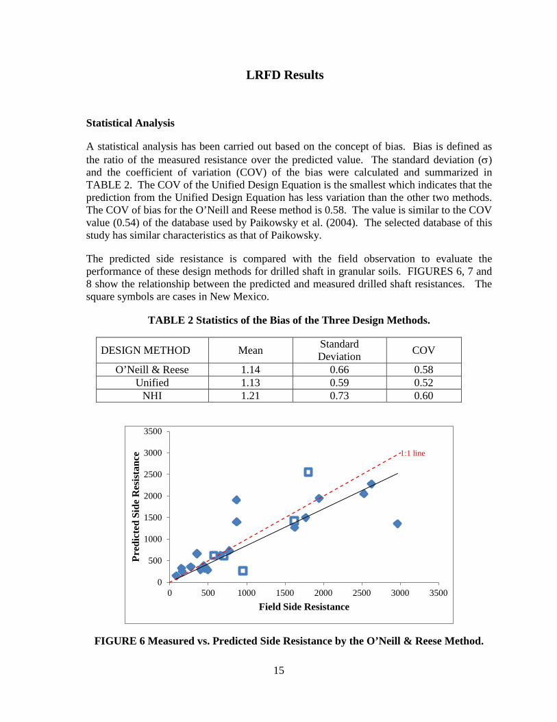
A statistical analysis has been carried out based on the concept of bias. Bias is defined as the ratio of the measured resistance over the predicted value. The standard deviation (σ) and the coefficient of variation (COV) of the bias were calculated and summarized in TABLE 2. The COV of the Unified Design Equation is the smallest which indicates that the prediction from the Unified Design Equation has less variation than the other two methods. The COV of bias for the O’Neill and Reese method is 0.58. The value is similar to the COV value (0.54) of the database used by Paikowsky et al. (2004). The selected database of this study has similar characteristics as that of Paikowsky.
The predicted side resistance is compared with the field observation to evaluate the performance of these design methods for drilled shaft in granular soils. FIGURES 6, 7 and 8 show the relationship between the predicted and measured drilled shaft resistances. The square symbols are cases in New Mexico.
TABLE 2 Statistics of the Bias of the Three Design Methods.
DESIGN METHOD Mean Standard Deviation COV
O’Neill & Reese 1.14 0.66 0.58 Unified 1.13 0.59 0.52
NHI 1.21 0.73 0.60
FIGURE 6 Measured vs. Predicted Side Resistance by the O’Neill & Reese Method.
0
500
1000
1500
2000
2500
3000
3500
0 500 1000 1500 2000 2500 3000 3500
Pred
icte
d Si
de R
esis
tanc
e
Field Side Resistance
1:1 line

16
FIGURE 7 Measured vs. Predicted Side Resistance by the Unified Design Method.
FIGURE 8 Measured vs. Predicted Side Resistance by the NHI Method.
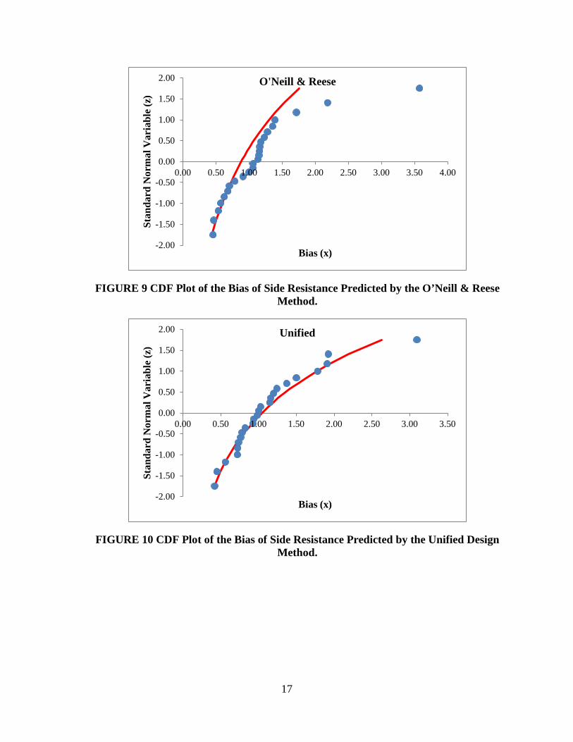
If the resistance bias is assumed to be lognormal distribution, the method of the best-fit-to-tail lognormal distribution recommended by Allen et al. (2005) is used. The statistical parameters shown in TABLE 2 cannot be used directly. Additional curve fitting is needed. FIGURES 9-11 show the cumulative distribution functions (CDF) of the bias of these three design equations as well as the curves of the best-fit-to-tail lognormal distributions.
0
500
1000
1500
2000
2500
3000
3500
0 500 1000 1500 2000 2500 3000 3500
Pred
icte
d Si
de R
esis
tanc
e
Field Side Resistance
1:1 line
0
500
1000
1500
2000
2500
3000
3500
0 500 1000 1500 2000 2500 3000 3500
Pred
icte
d Si
de R
esis
tanc
e
Field Side Resistance
1:1 line
17
FIGURE 9 CDF Plot of the Bias of Side Resistance Predicted by the O’Neill & Reese Method.
FIGURE 10 CDF Plot of the Bias of Side Resistance Predicted by the Unified Design Method.
-2.00
-1.50
-1.00
-0.50
0.00
0.50
1.00
1.50
2.00
0.00 0.50 1.00 1.50 2.00 2.50 3.00 3.50 4.00
Stan
dard
Nor
mal
Var
iabl
e (z
)
Bias (x)
O'Neill & Reese
-2.00
-1.50
-1.00
-0.50
0.00
0.50
1.00
1.50
2.00
0.00 0.50 1.00 1.50 2.00 2.50 3.00 3.50
Stan
dard
Nor
mal
Var
iabl
e (z
)
Bias (x)
Unified

18
FIGURE 11 CDF Plot of the Bias of Side Resistance Predicted by the NHI Method.
The mean, standard deviation, and COV of these best-fit-to-tail lognormal distributions of the design equations (curves in FIGURES 9-11) are listed in TABLE 3. They will be used in the LRFD calibration process and described in the later section.
TABLE 3 Statistics of the Bias of the Best-Fit-to-Tail Distributions.
DESIGN METHOD Mean Standard Deviation COV
O’Neill & Reese 0.95 0.39 0.41 Unified 1.2 0.68 0.57
NHI 0.88 0.31 0.35
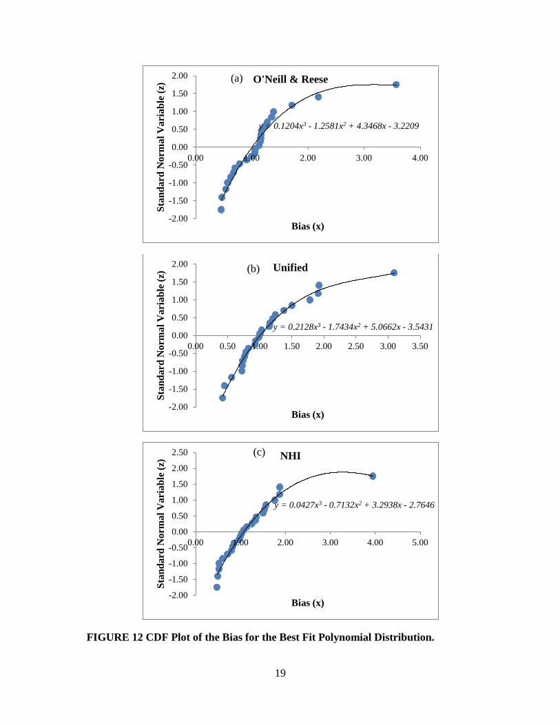
The CDF of the bias can also be fitted by polynomial curve. The best-fit polynomial curves (the solid curves) for the O’Neill & Reese method, the Unified design equation and the NHI equation are shown in FIGURE 12. The polynomial equations are also displayed in the figure. These polynomial equations are used to generate the random values of resistance in the Monte Carlo simulation.
The load (both dead load and live load) is assumed to be distributed lognormally. The statistical characteristics parameters of load components are the same as Paikowsky (2004).
The statistical parameters of live and dead loads are:
γLL = 1.75 λLL = 1.15 COVLL = 0.2
γDL = 1.25 λDL = 1.05 COVDL = 0.1
-2.00
-1.50
-1.00
-0.50
0.00
0.50
1.00
1.50
2.00
0.00 1.00 2.00 3.00 4.00 5.00
Stan
dard
Nor
mal
Var
iabl
e (z
)
Bias (x)
NHI
19
FIGURE 12 CDF Plot of the Bias for the Best Fit Polynomial Distribution.
y = 0.1204x3 - 1.2581x2 + 4.3468x - 3.2209
-2.00
-1.50
-1.00
-0.50
0.00
0.50
1.00
1.50
2.00
0.00 1.00 2.00 3.00 4.00St
anda
rd N
orm
al V
aria
ble
(z)
Bias (x)
O'Neill & Reese
y = 0.2128x3 - 1.7434x2 + 5.0662x - 3.5431
-2.00
-1.50
-1.00
-0.50
0.00
0.50
1.00
1.50
2.00
0.00 0.50 1.00 1.50 2.00 2.50 3.00 3.50
Stan
dard
Nor
mal
Var
iabl
e (z
)
Bias (x)
Unified
y = 0.0427x3 - 0.7132x2 + 3.2938x - 2.7646
-2.00
-1.50
-1.00
-0.50
0.00
0.50
1.00
1.50
2.00
2.50
0.00 1.00 2.00 3.00 4.00 5.00
Stan
dard
Nor
mal
Var
iabl
e (z
)
Bias (x)
NHI
(a)
(b)
(c)
20
Calibration of Resistance Factor (Monte Carlo Method)
When the resistance bias is assumed to be lognormal distribution, the Monte Carlo method used in this study is similar to the recommended procedures by the Transportation Research Circular E-C079 (Allen et al. 2005). Fifty thousand sets of random numbers for dead load, live load, and resistance are generated. The LL is set to 1 and the DL/LL is 3. Three random numbers, a, b, and c (0 < a, b, c < 1) are generated. The live load (LLrnd), dead load (DLrnd), and resistance (Rrnd) are calculated based on the random numbers as:
LLrnd= exp(µIn + a*σ in) DLrnd= exp(µIn + b*σ in) Rrnd=exp(µIn +c*σ in) σ in=(ln(COV²Q +1))0.5
σ in=(ln(COV²R +1))0.5
µIn= In(µQ*(LL)-0.5*σ in
2
µIn= In(µQ*(LL*DL/LL)-0.5*σ in2
µIn= In(µR*(LL*γLL +DL*γ DL)/ф)-0.5*σ in
(24)
For a probability of failure of 1 in 1000, the resistance factors for the O’Neill and Reese method, the Unified design equation, and the NHI design method, are found to be 0.32, 0.26, and 0.37, respectively. The resistance factor for the Unified design equation is the smallest due to the highest COV value of the best-fit-to-tail lognormal distribution (see Table 3). The value is greater than the value (0.2) reported by Murad et al. (2010). The resistance factor is in good agreement with the reported value (0.31) by Paikowsky et al. (2004).
When the CDF of the resistance bias is modeled as a polynomial curve, the calibrated resistance factors obtained from Monte Carlo simulations are 0.45, 0.49, and 0.47 for the O’Neill and Reese Method, the Unified design equation, and the NHI design equation, respectively. These resistance factors are very similar. These resistance factors are greater than those determined assuming the resistance bias is lognormally distributed. Since the CDF of the resistance bias is not lognormal, the curve fitted polynomial regression model is more rational.

21
The Discrete Element Analysis
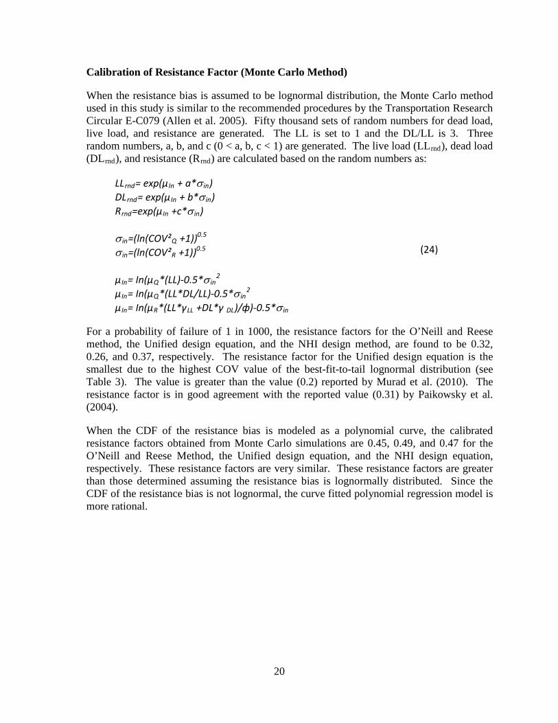
The discrete element method (DEM) is used to simulate the mobilization of the side resistance of a drilled shaft. Details of the method can be obtained in literature (Cundall and Strack 1979). FIGURE 13 shows a typical system. Two different types of boundary conditions are used. Rigid planar surfaces are at the top and bottom and at the front and back surfaces. Periodic boundaries along the azimuth direction are used to reduce the sample size.
Granular soils are modeled as assemblies of particles. Particles are created randomly. 1-D compression is then applied to densify the system. No lateral displacement is allowed. During the sample preparation stage, the friction coefficient is set to zero at the rigid planar boundaries. Uniform stress is observed in these samples. When frictional rigid boundaries are used, the stress distribution inside the sample becomes non-uniform. The non-uniform stress distribution is due to the development of arching from the top surface to the bottom surface during the compression stage. Therefore, frictionless boundaries are used during the compression stage.
In order to create samples of different initial densities, samples are compressed first with a friction coefficient between particles of 0.1 to a desired void ratio. The compression is stopped when the intermediate system has a void ratio of 0.8, 0.75, 0.7, 0.65, and 0.6. The vertical stresses of these intermediate systems are less than 200 psf. Then, the friction coefficient is set to 0.5 and the system is compressed again to a vertical stress of 2000 psf. The horizontal stresses of the final systems are measured. Five different samples are created. The void ratios of these final samples are 0.710, 0.685, 0.646, 0.622, and 0.597. The horizontal stresses in the two horizontal directions vary slightly. The ratio of the average horizontal stress and vertical stress is defined as the at rest earth pressure coefficient (Ko). The Ko of these samples are 0.730, 0.630, 0.439, 0.401, and 0.432 respectively. Ko decreases as the density of the sample increases except for the very dense sample.
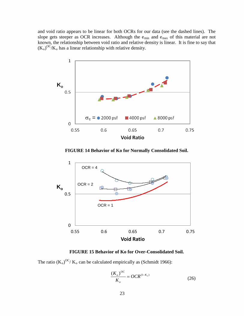
These five samples are further compressed to two other vertical stresses (4000 psf and 8000 psf). FIGURE 14 plots the Ko of these 15 samples. The result shows that the effect of vertical stress is negligible. Ko is a function of void ratio only. This is in agreement with the laboratory results on sands (Mesri and Vardhanabhuti, 2009). The DEM result shows that Ko reaches an asymptotic value (≈ 0.4) as void ratio (e) decreases. More data is needed to clarify this finding. A trend line can be defined for these normally consolidated samples. The equation of the trend line is given as:
Ko = 26.696e2 - 32.264e + 10.144 (25)
Overconsolidated samples are prepared by reducing the vertical stress of some normally consolidated samples. Two overconsolidation ratios (OCR) are selected. OCR is the ratio of maximum past consolidation pressure and the current vertical stress. The at rest earth pressure coefficient of these overconsolidated samples, (Ko)OC, is plotted in FIGURE 15. The superscript indicates the overconsolidated state. The behavior of normally consolidated samples (Eq. 25) is also plotted in the figure for comparision. The open symbols are OC
22
samples developed from the samples with a maximum past pressure of 8000 psf. The filled symbols are for the samples with a maximum past pressure of 4000 psf. Circle symbols are for samples with current vertical stress of 2000 psf. Square symbols are for samples with current vertical stress of 4000 psf. As expected, (Ko)OC is greater than Ko. The degree of increase in Ko with OCR is a function of void ratio. For samples of lower density (higher void ratio), the effect of OCR is less profound than those of dense samples (lower void ratio). Comparing the filled circle symbols (σv’ = 2000 psf) and square symbols (σv’ = 4000 psf) for OCR = 2, (Ko)OC indicates that the effect of current vertical stress is insignificant. This is similar to the observation for normally consolidation samples (OCR = 1).
FIGURE 13 A Numerical System used to simulate the Mobilization of Side Resistance.
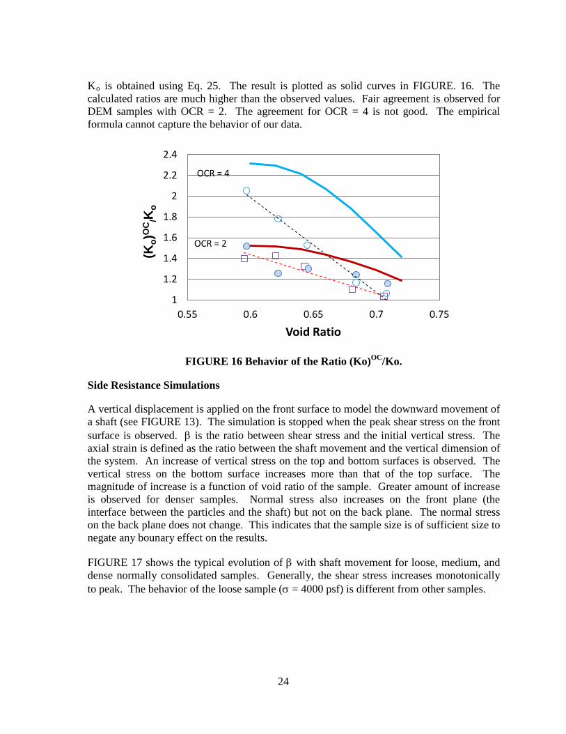
Another way to examine the effect of OCR is to plot the ratio of (Ko)OC and Ko versus void ratio as shown in FIGURE 16. The DEM result is plotted as symbols. The solid curves are obtained using an empirical formula. The ratio ((Ko)OC/Ko) decreases with the increase of void ratio (or the decrease of the density of a sample). The relationship between (Ko)OC/Ko
23
and void ratio appears to be linear for both OCRs for our data (see the dashed lines). The slope gets steeper as OCR increases. Although the emin and emax of this material are not known, the relationship between void ratio and relative density is linear. It is fine to say that (Ko)OC/Ko has a linear relationship with relative density.
FIGURE 14 Behavior of Ko for Normally Consolidated Soil.
FIGURE 15 Behavior of Ko for Over-Consolidated Soil.
The ratio (Ko)OC/ Ko can be calculated empirically as (Schmidt 1966):
)1()(oK
o
OCo OCRK
K −=
(26)
0
0.5
1
0.55 0.6 0.65 0.7 0.75
Ko
Void Ratio
OCR = 4
OCR = 2
OCR = 1
σc =
24
Ko is obtained using Eq. 25. The result is plotted as solid curves in FIGURE. 16. The calculated ratios are much higher than the observed values. Fair agreement is observed for DEM samples with OCR = 2. The agreement for OCR = 4 is not good. The empirical formula cannot capture the behavior of our data.
FIGURE 16 Behavior of the Ratio (Ko)OC/Ko.
Side Resistance Simulations
A vertical displacement is applied on the front surface to model the downward movement of a shaft (see FIGURE 13). The simulation is stopped when the peak shear stress on the front surface is observed. β is the ratio between shear stress and the initial vertical stress. The axial strain is defined as the ratio between the shaft movement and the vertical dimension of the system. An increase of vertical stress on the top and bottom surfaces is observed. The vertical stress on the bottom surface increases more than that of the top surface. The magnitude of increase is a function of void ratio of the sample. Greater amount of increase is observed for denser samples. Normal stress also increases on the front plane (the interface between the particles and the shaft) but not on the back plane. The normal stress on the back plane does not change. This indicates that the sample size is of sufficient size to negate any bounary effect on the results.
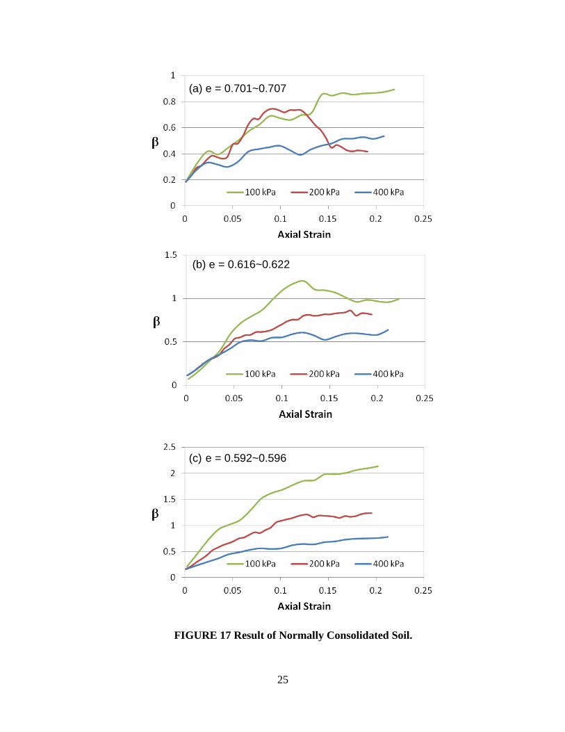
FIGURE 17 shows the typical evolution of β with shaft movement for loose, medium, and dense normally consolidated samples. Generally, the shear stress increases monotonically to peak. The behavior of the loose sample (σ = 4000 psf) is different from other samples.
1
1.2
1.4
1.6
1.8
2
2.2
2.4
0.55 0.6 0.65 0.7 0.75
(Ko)
OC
/Ko
Void Ratio
OCR = 2
OCR = 4
25
FIGURE 17 Result of Normally Consolidated Soil.
(a) e = 0.701~0.707
(b) e = 0.616~0.622
(c) e = 0.592~0.596
26
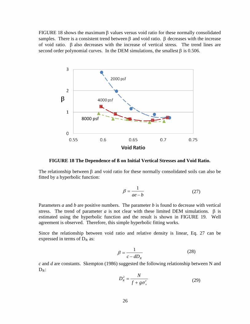
FIGURE 18 shows the maximum β values versus void ratio for these normally consolidated samples. There is a consistent trend between β and void ratio. β decreases with the increase of void ratio. β also decreases with the increase of vertical stress. The trend lines are second order polynomial curves. In the DEM simulations, the smallest β is 0.506.
FIGURE 18 The Dependence of ß on Initial Vertical Stresses and Void Ratio.
The relationship between β and void ratio for these normally consolidated soils can also be fitted by a hyperbolic function:
bae −
=1β (27)
Parameters a and b are positive numbers. The parameter b is found to decrease with vertical stress. The trend of parameter a is not clear with these limited DEM simulations. β is estimated using the hyperbolic function and the result is shown in FIGURE 19. Well agreement is observed. Therefore, this simple hyperbolic fitting works.
Since the relationship between void ratio and relative density is linear, Eq. 27 can be expressed in terms of DR as:
RdDc −
=1β (28)
c and d are constants. Skempton (1986) suggested the following relationship between N and DR:
v
R gfND
σ ′+=2
(29)
8000 psf

27
where f and g are constants. σ’v is the effective overburden stress in atm (1 tsf).
Finally, β is a function of σ’v and N. Another phenomenological model can be developed.
FIGURE 19 Comparison between the Hyperbolic Curve Fitting and Observed Data.
DEM simulations are compared with the prediction of the Unified design equation and the NHI method. For the Unified design equation, depth (z) is required to calculate β as shown in Eq. 30. For vertical stresses of 2000, 4000, and 8000 psf, the depths are equal to approximately 17 ft, 34 ft, and 68 ft, respectively. β is estimated as:
+
−+=
z
KKK op
oU 1tanφβ
(30)
Ko is obtained using Eq. 25 for a given void ratio. φ is calculated as:
)1(sin 1
oK−= −φ
(31)
In the NHI method, the vertical stress has no effect since the samples are normally consolidated. Equation 8 becomes:
φβ tanoF K= (32)
These predicted βs are shown in Figure 20. The dashed curves are obtained from the Unified design equation. The solid curve is for the NHI method. The estimated β from both design equations is smaller than the DEM data. β estimated by these design equations
0
1
2
3
0.55 0.6 0.65 0.7 0.75
β
Void Ratio
8000 psf
4000 psf
2000 psf

28
shows an increasing rate with the increase of void ratio. The numerical simulations show a decreasing rate (see FIGURE 19).
FIGURE 20 Behavior of β with the Predicted Equations.
The DEM simulations show that a larger decrease of β occurs when the vertical stress increases from 2000 psf to 4000 psf. A smaller decrease of β occurs when the vertical stress increases from 4000 psf to 8000 psf. The NHI method is not a function of vertical stress for normally consolidated soils. The Unified design equation predicts a similar amount of decrease in β from 4000 psf to 8000 psf as that from 2000 psf to 4000 psf.
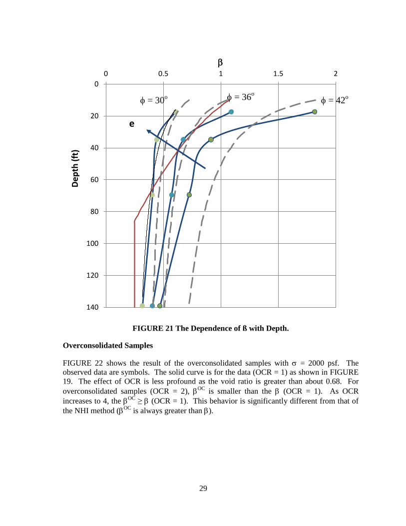
The relation between β and depth from the numerical observation is plotted in Figure 21, together with the behaviors of the O’Neill method and of the Unified design equation. The red line is for the O’Neill and Reese method. The dashed curves are for the Unified design equation for loose (φ = 30°), medium dense (φ = 36°) and dense (φ = 42°) sands. The solid curves with symbols are the DEM numerical result. The curve shifts to the left as void ratio increases. The DEM result shows a rapid reduction of β for depth above 40 ft. A linear reduction of β can be approximated below 40 ft.
FIGURE 21 indicates that the Unified design equation does capture some effect of depth. Greater similarity is found for loose and medium dense sands between the Unified design equation and DEM observation. However, the reduction of β with depth is much greater than the square root of depth as in Eq. 12. The DEM indicates that the reduction rate of β with depth is a function of the friction angle (void ratio). This may explain the good performance of the NHI method. The equation does contain a power index of sinφ (see Eq. 5). However, this is not the OCR effect as considered in the NHI method since the DEM models are normally consolidated.
0
0.2
0.4
0.6
0.8
1
1.2
0.55 0.6 0.65 0.7 0.75
β
Void Ratio
NHI
8000 psf
4000 psf
2000 psf Unified method
29
FIGURE 21 The Dependence of ß with Depth.
Overconsolidated Samples
FIGURE 22 shows the result of the overconsolidated samples with σ = 2000 psf. The observed data are symbols. The solid curve is for the data (OCR = 1) as shown in FIGURE 19. The effect of OCR is less profound as the void ratio is greater than about 0.68. For overconsolidated samples (OCR = 2), βOC is smaller than the β (OCR = 1). As OCR increases to 4, the βOC ≥ β (OCR = 1). This behavior is significantly different from that of the NHI method (βOC is always greater than β).
0
20
40
60
80
100
120
140
0 0.5 1 1.5 2De
pth
(ft)
β
φ = 30o φ = 36o φ = 42o
e

30
FIGURE 22 Result of Overconsolidated Samples (σ = 2000 psf).
FIGURE 23 shows the result of overconsolidated samples (OCR = 2) with various vertical stresses (σ = 2000 psf to 4000 psf). Although the vertical stress does not affect the trend between β and void ratio, it affects the magnitude of β slightly. This is different from the behavior of normally consolidated samples as the vertical stress affects both the trend and the magnitude.
FIGURE 23 Result of Overconsolidated Samples (OCR = 2).
0
1
2
3
4
0.55 0.6 0.65 0.7 0.75
βOC
Void Ratio
0
1
2
3
0.55 0.6 0.65 0.7 0.75
β
Void Ratio
OCR = 4
OCR = 2
σ = 2000 psf
σ = 4000 psf
31
Conclusions and Implementation Plan
In this study, the side resistance factor for drilled shafts in granular soils was calibrated on the basis of the statistical data. Based on the current data set, the resistance factor of 0.32 (using best fit-to-tail lognormal distribution) is determined for the O’Neill and Reese Method. The value is greater than the value (0.2) reported by Murad et al. (2010) for case histories around Louisiana. The resistance factor is in good agreement with the reported value (0.31) by Paikowsky et al. (2004) for case histories in the US. This indicates that the selected database for this study is compatible with that of Paikowsky et al.
When the cumulative distribution function of the resistance bias is described by a polynomial curve, the calibrated resistance factors are 0.45, 0.49, and 0.47 for the O’Neill and Reese Method, the Unified design equation, and the NHI design equation, respectively. The resistance factors for these three design equations are still less than the 0.55 (recommended for the O’Neill and Reese method). The results show that the resistance factor for the Unified design equation (0.49) is greater than that for the O’Neill and Reese method (0.45). It is reasonable to suggest that a similar resistance factor (0.55) could be suggested for the Unified Design Equation. However, further study should be carried out to confirm the resistance factor.
The DEM result has shown that the relationship between β and void ratio (relative density) is quite complicated. β is a function of relative density, vertical stress, and OCR. For normally consolidated samples, a simple hyperbolic curve can describe the relationship between β and void ratio. The effect of OCR on β is not clear. More DEM data is needed to identify the role of OCR.
Differences between the DEM simulations and the predicated equations are observed. Both the Unified design equation and the NHI method partially capture the effect of depth on β. The effect of vertical stress cannot be represented by the reciprocal of the square root of depth. Other functions should be used. In the NHI equation, the effect of OCR is attempted. However, the DEM data show that the effect of OCR on β is different from that of the NHI equation. Although conclusive result of OCR cannot be obtained due to the limited DEM simulations in this study, the Unified design equation should incorporate an OCR term.
It is suggested to carry out more DEM simulations to clearly identify the trend of certain factors. Then, modify the Unified design equation based on the DEM simulations. The uncertainty of predicted resistance could be reduced (a smaller COV). Finally, a higher resistance factor can be determined from the reliability analysis.
Implementation Plan
The research result has shown great promise in the development of a design equation for drilled shafts. It indicates the possibility of developing a cost saving scheme for drilled shaft design. The goal can be achieved by modifying the Unified design equation with the help of DEM simulations and by collecting more case histories from New Mexico.

32
It is recommended to continue this research effort to the next phase to achieve fruitful result. The expected product is a better design equation that will produce a more reliable design side resistance in granular soils. This will provide cost savings to the NMDOT. Suggested Framework for Future Study • Use a spreadsheet to develop nominal resistance on selected NMDOT STIP projects with the recommended resistance factors • Develop cost comparison of each method for factored resistances required • Develop fully instrumented load testing on selected projects to enhance the NMDOT database • Compare load test results with computed nominal resistance of each method • Recalibrate Unified Equation resistance factor utilizing additional database from load tests • Document cost savings of each project for Unified Equation as compared to other design methods

33
References
Abu-Farsakh, M.Y, X. Yu, S. Yoon, and C. Tsai. Calibration of Resistance Factors Needed in the LRFD Design of Drilled Shafts. FHWA/LA.10, 2010, pp. 470.
AbdelSalam, S., K. Ng, S. Sritharan, M. Suleiman, and M. Roling. Development of LRFD Procedures for Bridge Pile Foundations. Volume III: Recommended Resistance Factors with Consideration of Construction Control and Setup. Ames, IA: Iowa State University – Institute for Transportation, 2012.
AbdelSalam, S., S. Sritharan, M. Suleiman, LRFD Resistance Factors for Design of Driven H-Piles in Layered Soils. ASCE Journal of Bridge Engineering, 2011, 16(6): pp. 729-748.
Ackerman, A.F. and J.C. Niedzielski. Draft Demonstration Drilled Shaft Installation and Static Load Testing Report for US-70 over Gila River Bridge. Gannett Fleming Inc., 2011, pp. 215.
Allen, T., A. Nowak, and R. Bathurst. Calibration to Determine Load and Resistance Factors for Geotechnical and Structural Design, TRB Circular Number E-C079, Transportation Research Board, Washington, DC, 2005.
AASHTO. LRFD Bridge Design Specifications. 3d Edition, American Association of State Highway and Transportation Officials, Washington, D.C., USA, 2004, pp. 582.
Bullock, J. Paul. A Study of the Setup Behavior of Drilled Shafts, Final Report for Florida Department of Transportation, 2003.
Burch, S.B., F. Parra, F.C. Townsend and M.C. McVay. Design Guidelines for Drilled Shaft Foundations. Univ. of Florida, Gainesville, 1988, pp. 141.
Chua, K.M., W.A.N. Asper, and R. Meyers. Testing and Predicting the Movement of a Drilled Shaft in New Mexico. Foundations and Embankments Deformations. Geotechnical Special Publication No. 40, 1994, pp. 279-291.
Chua, K.M., R. Meyers, and N. Samtani. Evolution of a Load Test and Finite Element Analysis of Drilled Shafts in Stiff Soils. ASCE GeoDenver, Denver, CO, 2000.
Chua, K.M. and R. Meyers. A Unified Design Equation for Cylindrical Drilled Shafts in Compression. Deep Foundations 2002: An International Perspective on Theory, Design, Construction, and Performance, GSP No. 116, 2002, pp. 1550-1566
Cundall, P.A. and O. Strack, O. A discrete numerical model for granular assemblies. Geotechnique, London, 29(1), 1979, 47-65.
Duncan, J. M.,P. Byrne, K.S. Wong, and P. Mabry. Strength, Stress-Strain and Bulk Modulus Parameters for Finite Element Analysis of Stresses And Movements in Soil Masses. Report No. UCB/GT/80-01, Dept. Civil Engineering, U.C. Berkeley, 1980.

34
Federal Highway Administration (FHWA). Drilled Shafts: Construction Procedures and LRFD Design Methods. FHWA-NHI-10-016, Washington, D.C., 2010.
Federal Highway Administration (FHWA). Drilled Shafts: Construction Procedures and Design Methods. by Reese, L. C. and O’Neil, M. W., for Federal Highway Administration, FHWA Report No. FHWA-HI-88-042, 1988.
Gibbs, H.J. and W.G. Holts. Resarch on determining the relative density of sands by spoon penetration testing. Proc. 4th Intl. Conference on Soil Mech. And Foundation Engineering, 1957, pp. 35-39
HDR. Load Test Report: I-10/SR 303L System Interchange in Maricopa County, Arizona, 2010, pp. 349.
ISRM (1987). Suggested Methods for Deformability Determination Using a Flexible Dilatometer.
Kulhawy, F.H. and J.R. Chen. Discussion of ‘Drilled Shaft Side Resistance in Gravelly Soils’ by Rollins, Clayton, Mikesell, and Blaise. Journal of Geotechnical and Geoenvironmental Engineering, ASCE, Vol. 133, No. 10, 2007, pp. 1325-1328.
Liang, R. and J. Li. Resistance Factors Calibrated from FHWA Drilled Shafts Static Top-Down Test Data Base. GSP 186: Contemporary Topics in In-Situ Testing, analysis, and Reliability of Foundations, 2009.
Mayne, P.W. In-Situ Test Calibrations for Evaluating Soil Parameters. Characterisation and Engineering Properties of Natural Soils, Vol. 3, Eds. Tan, Phoon, Hight, and Leroueil, 2007, pp. 1601-1652
McVay, M.C., R.D. Ellis, M. Kim, J. Villegas, S.-H. Kim, and S. Lee. Static and Dynamic Field testing of Drilled Shafts: suggested guidelines on their use for FDOT structures. WPI No. BC354-08. Final Report 4910-4504-725-12, 2003, pp. 303.
Mesri, G. and B. Vardhanabhuti. Compression of Granular Materials. Canadian Geotechnical Journal. 46, 2009, pp. 369-392.
Murad Y. Abu-Farsakh, X. Yu, S. Yoon, and C. Tsi. Calibration of Resistance Factors needed in the LRFD design of Drilled Shafts. Report No: FHWA/LA. 10/470. Louisiana Department of Transportation and Development, Louisiana, 2010.
New Mexico Department of Transportation. Final report on drilled shaft load testing (Osterberg method) NM 74 over Rio Grande, 1995.
New Mexico Department of Transportation. Load test report: Drilled shaft load test project, Big I project, I25/I40 system interchange, Albuquerque, NM, 1999.

35
Noriyuki, Y. and H. Ochiai. Skin Friction of Non-Displacement Piles Related to Simple Shear Mode with Large Strain State Friction Angle. Soils and foundations, Vol. 46, No. 4, Aug. 2006, pp. 537-544.
Nowak, A.S. Calibration of LRFD Bridge Design code. NCHRP Report 368, TRB, National Academy Press, Washington, DC, 1999.
Nusairat, J., R.Y. Liang, and R.L. Engel. Verification and Calibration of the Design Methods for Rock Socketed Drilled Shafts for Lateral Loads. Final Report. Columbus, OH: E.L. Robinson Engineering of Ohio, Co, 2011.
O’Neill, M. W. and L.C. Reese, L. C. Drilled Shafts: Construction Procedures and Design Methods. Report No. FHWA-IF-99-025, FHWA, 1999.
O'Neill, M.W. and L.C. Reese. Load Transfer in a Slender Drilled Pier in Sand. Preprint 3141, ASCE Spring Convention, Pittsburgh, 1978, pp. 30.
O’Neill, M., F. Townsend, K. Hassan, A. Buller, and P. Chang. Load Transfer for Drilled Shafts in Intermediate Geomaterials. FHWA-RD-95-172, FHWA, 1996, pp. 184.
O'Neill, M.W. and K.M. Hassan. Drilled Shafts: Effects of Construction on Performance and Design Criteria. Proceedings of the International Conference on Design and Construction of Deep Foundations, December 1994, Vol. 1, 1994, pp. 137-187.
Owens, M.J. and L.C. Reese. The Influence of a Steel Casing on the Axial Capacity of a Drilled Shaft. Research report 255-1F, Report to the Texas State Depatment of Highways and Public Transportation Center for Transportation research, Bueau of Engineering Research, The niversity of Texas at Austin, Austin, Tesas, July, 1982, pp.204.
Paikowsky, S.G., with contributions from B. Birgisson, M. McVay, T. Nguyen, C. Kuo, G. Baecher, B. Ayyub, K. Stenersen, K. O.Malley, L. Chernauskas, and M. O’Neill, Load and Resistance Factor Design (LRFD) for Deep Foundations. NCHRP Report 507, Transportation Research Board, Washington, DC, 2004, pp. 126.
Pizzi, J. F. Case History: Capacity of a Drilled Shaft in the Atlantic Coastal Plain. Journal of Geotechnical and Geoenvironmental Engineering, Vol. 133, No. 5, 2007, pp. 522-530.
Reese, L.G. and M.W. O'Neill. Field Load Tests of Drilled Shafts. Proceedings, 1st Intl. Geotechnical seminar on deep foundations on bored and auger piles, Ghent, 1988, pp. 145-191.
Reese, L.C. and S.J. Wright. Construction Procedure and Design for Axial Loading. Vol. 1, Drilled shaft manual, HDV-22, Implementation Package 77-21, Implementation Division, U.S. Department of Transportation, McLean, Virginia, 1977, pp. 140.

36
Schmidt, B. Earth Pressures at Rest Related to Stress History Discussion. Canadian Geotechnical Journal, 3(4), 1966, pp. 239-242.
Skempton, A.W. Standard penetration test procedures and effects in sands of overburden pressure, relative density, particle size, aging and overconsolidation, Geotechnique, 36(3), 1986, pp. 425-447.
Simpson, R.C. Report on Drilled Shaft Load Testing (Osterberg method): SR24 SR 202L to Ellsworth road-Mesa, AZ, Loadtest Inc., 2011, pp. 113.
Simpson, R.C. Load Test Report: Test Shaft 1 - San Carlos River Bridge, Loadtest Inc., 2010, pp. 84.
Simpson, R.C. Report on Drilled Shaft Load Testing (Osterberg method): Sky Harbor International Airport, TS -1, Loadtest Inc., 2008, pp. 76.
Simpson, R.C. Report on Drilled Shaft Load Testing (Osterberg method): TS -1, Sunland Park Drive, Sunland Park, NM, Loadtest Inc., 2006, pp. 70.
Soil and Material Engineers, Inc. Elementary Geotechnical Foundation Report, Proposed Office Building. Prepared for Wilma southest corporation, Atlanta, Georgia, March, 1984.
U.S. Navy . Soil Mechanics, Foundations and Earth Structures. NAVFAC Design Manual DM-7, Washington. D.C., 1971.
Van Foeken, R.J. and G. Jonker. Bottom Driving Casing Technique Predictions with TNOWAVE. Deep foundations 2002, Vol. 1, 2002, pp. 351-362.
Waisnor, B. M., A. Ducote-Price, B. Jarosz, J. Duncan, and C.J. Smith. Geotechnical Engineering within the Piedmont Physiographic Province. Report of a study performed by the Virginia Tech Center for Geotechnical Practice and Research, 2001, pp. 27.
Wang, Y.Z. Design and Construction of Large Bored Piles over Yellow River, Proceedings, International Conference on Deep Foundations, Beijing, 1986, pp. 124-129.
Withiam, J.L., E.P. Voytko, R.M. Barker, J.M. Duncan, B.C. Kelly, S.C. Musser, and V. Elias. Load and Resistance Factor Design (LRFD) for Highway Bridge Substructures. FHWA HI-98-032, FHWA, Washington DC, 1998.
Wolff, T.E. Pile Capacity Prediction Using Parameter Functions. ASCE Geotechnical Special Publication, No. 23, 1989, pp. 96-107.
Yang, X., J. Han, R. Parsons, and R. Henthorne. Resistance Factors for Drilled Shafts in Weak Rocks Based on O-Cell Test Data. Transportation Research Record 2045. Transportation Research Board, National Research Council, Washington, D.C., 2008, pp. 62-67.
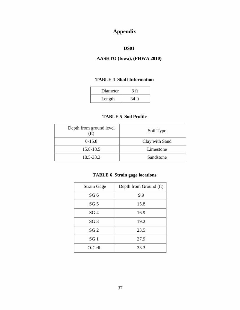
37
Appendix
DS01
AASHTO (Iowa), (FHWA 2010)
TABLE 4 Shaft Information
Diameter 3 ft
Length 34 ft
TABLE 5 Soil Profile
Depth from ground level (ft) Soil Type
0-15.8 Clay with Sand
15.8-18.5 Limestone
18.5-33.3 Sandstone
TABLE 6 Strain gage locations
Strain Gage Depth from Ground (ft)
SG 6 9.9
SG 5 15.8
SG 4 16.9
SG 3 19.2
SG 2 23.5
SG 1 27.9
O-Cell 33.3
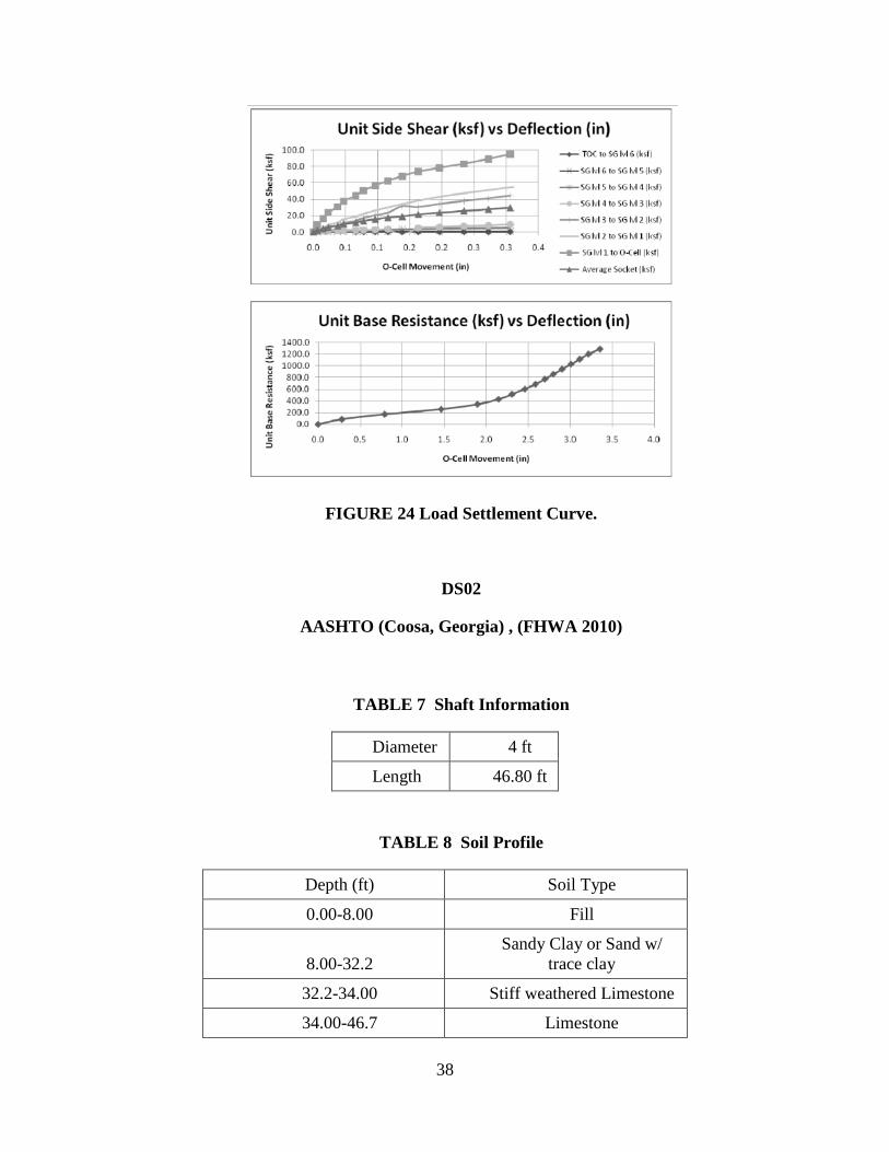
38
FIGURE 24 Load Settlement Curve.
DS02
AASHTO (Coosa, Georgia) , (FHWA 2010)
TABLE 7 Shaft Information
Diameter 4 ft
Length 46.80 ft
TABLE 8 Soil Profile
Depth (ft) Soil Type
0.00-8.00 Fill
8.00-32.2 Sandy Clay or Sand w/
trace clay
32.2-34.00 Stiff weathered Limestone
34.00-46.7 Limestone
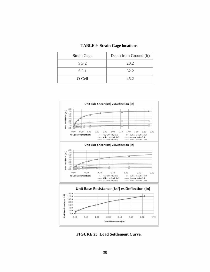
39
TABLE 9 Strain Gage locations
Strain Gage Depth from Ground (ft)
SG 2 20.2
SG 1 32.2
O-Cell 45.2
FIGURE 25 Load Settlement Curve.
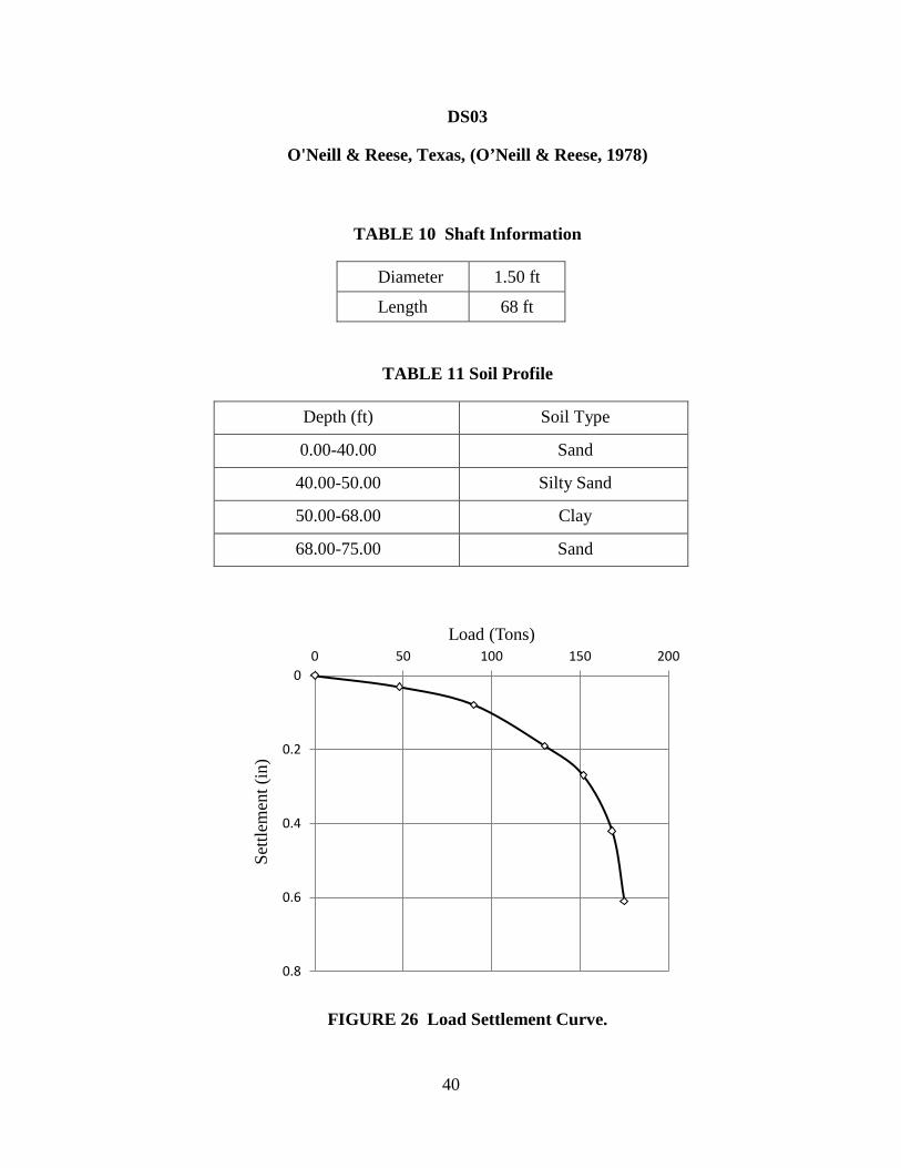
40
DS03
O'Neill & Reese, Texas, (O’Neill & Reese, 1978)
TABLE 10 Shaft Information
Diameter 1.50 ft
Length 68 ft
TABLE 11 Soil Profile
Depth (ft) Soil Type
0.00-40.00 Sand
40.00-50.00 Silty Sand
50.00-68.00 Clay
68.00-75.00 Sand
FIGURE 26 Load Settlement Curve.
0
0.2
0.4
0.6
0.8
0 50 100 150 200
Settl
emen
t (in
)
Load (Tons)
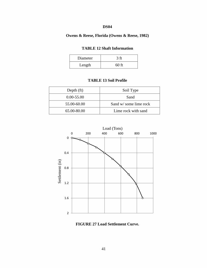
41
DS04
Owens & Reese, Florida (Owens & Reese, 1982)
TABLE 12 Shaft Information
Diameter 3 ft
Length 60 ft
TABLE 13 Soil Profile
FIGURE 27 Load Settlement Curve.
0
0.4
0.8
1.2
1.6
2
0 200 400 600 800 1000
Settl
emen
t (in
)
Load (Tons)
Depth (ft) Soil Type
0.00-55.00 Sand
55.00-60.00 Sand w/ some lime rock
65.00-80.00 Lime rock with sand
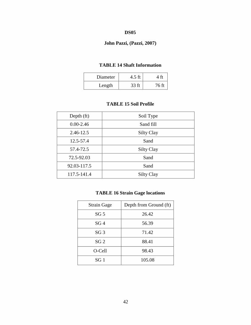
42
DS05
John Pazzi, (Pazzi, 2007)
TABLE 14 Shaft Information
Diameter 4.5 ft 4 ft
Length 33 ft 76 ft
TABLE 15 Soil Profile
Depth (ft) Soil Type
0.00-2.46 Sand fill
2.46-12.5 Silty Clay
12.5-57.4 Sand
57.4-72.5 Silty Clay
72.5-92.03 Sand
92.03-117.5 Sand
117.5-141.4 Silty Clay
TABLE 16 Strain Gage locations
Strain Gage Depth from Ground (ft)
SG 5 26.42
SG 4 56.39
SG 3 71.42
SG 2 88.41
O-Cell 98.43
SG 1 105.08
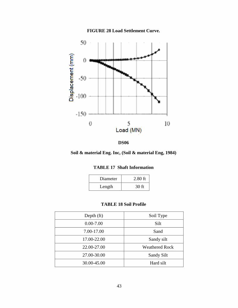
43
FIGURE 28 Load Settlement Curve.
DS06
Soil & material Eng. Inc, (Soil & material Eng, 1984)
TABLE 17 Shaft Information
Diameter 2.80 ft
Length 30 ft
TABLE 18 Soil Profile
Depth (ft) Soil Type
0.00-7.00 Silt
7.00-17.00 Sand
17.00-22.00 Sandy silt
22.00-27.00 Weathered Rock
27.00-30.00 Sandy Silt
30.00-45.00 Hard silt
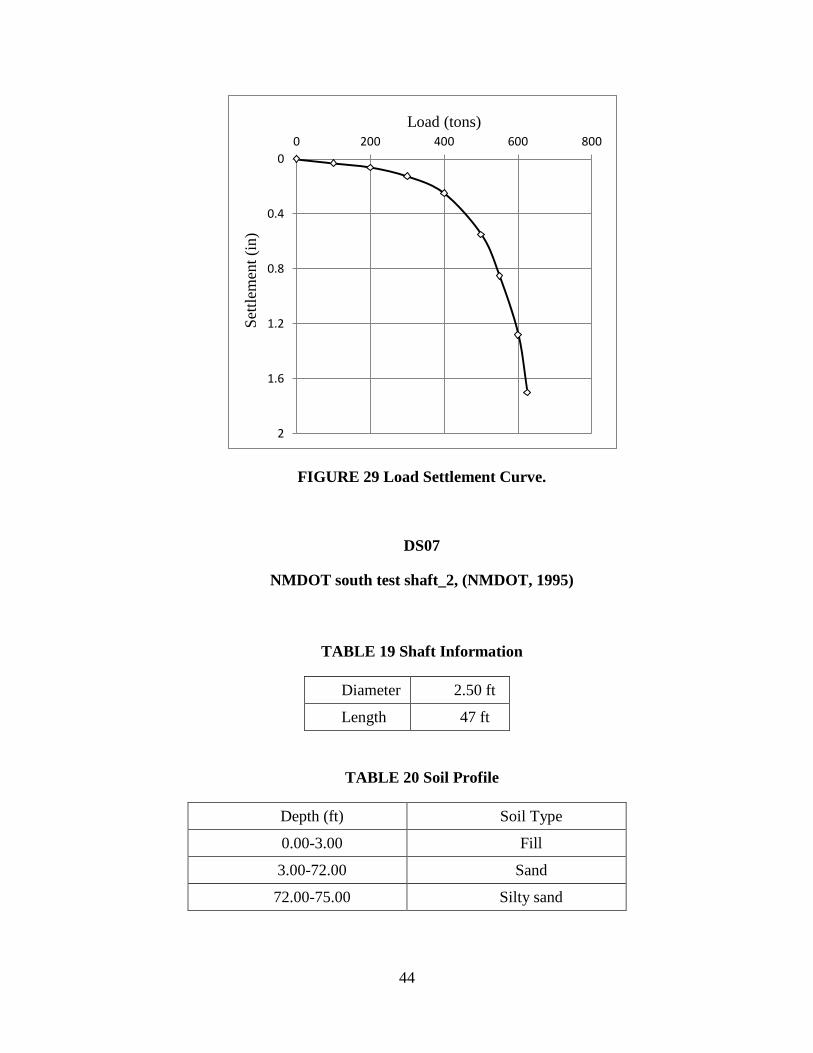
44
FIGURE 29 Load Settlement Curve.
DS07
NMDOT south test shaft_2, (NMDOT, 1995)
TABLE 19 Shaft Information
Diameter 2.50 ft
Length 47 ft
TABLE 20 Soil Profile
Depth (ft) Soil Type
0.00-3.00 Fill
3.00-72.00 Sand
72.00-75.00 Silty sand
0
0.4
0.8
1.2
1.6
2
0 200 400 600 800
Settl
emen
t (in
)
Load (tons)
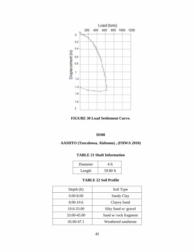
45
FIGURE 30 Load Settlement Curve.
DS08
AASHTO (Tuscaloosa, Alabama) , (FHWA 2010)
TABLE 21 Shaft Information
Diameter 4 ft
Length 59.80 ft
TABLE 22 Soil Profile
Depth (ft) Soil Type
0.00-8.00 Sandy Clay
8.00-10.6 Clayey Sand
10.6-33.00 Silty Sand w/ gravel
33.00-45.00 Sand w/ rock fragment
45.00-47.1 Weathered sandstone

46
TABLE 23 Strain Gage locations
Strain Gage Depth from Ground (ft)
SG 2 30.3
SG 1 45.6
O-Cell 57.6
FIGURE 31 Load Settlement Curve.
DS09
Big I, Albuquerque (L-1), (NMDOT, 1999)
TABLE 24 Shaft Information
Diameter 4.50 ft
Length 52 ft
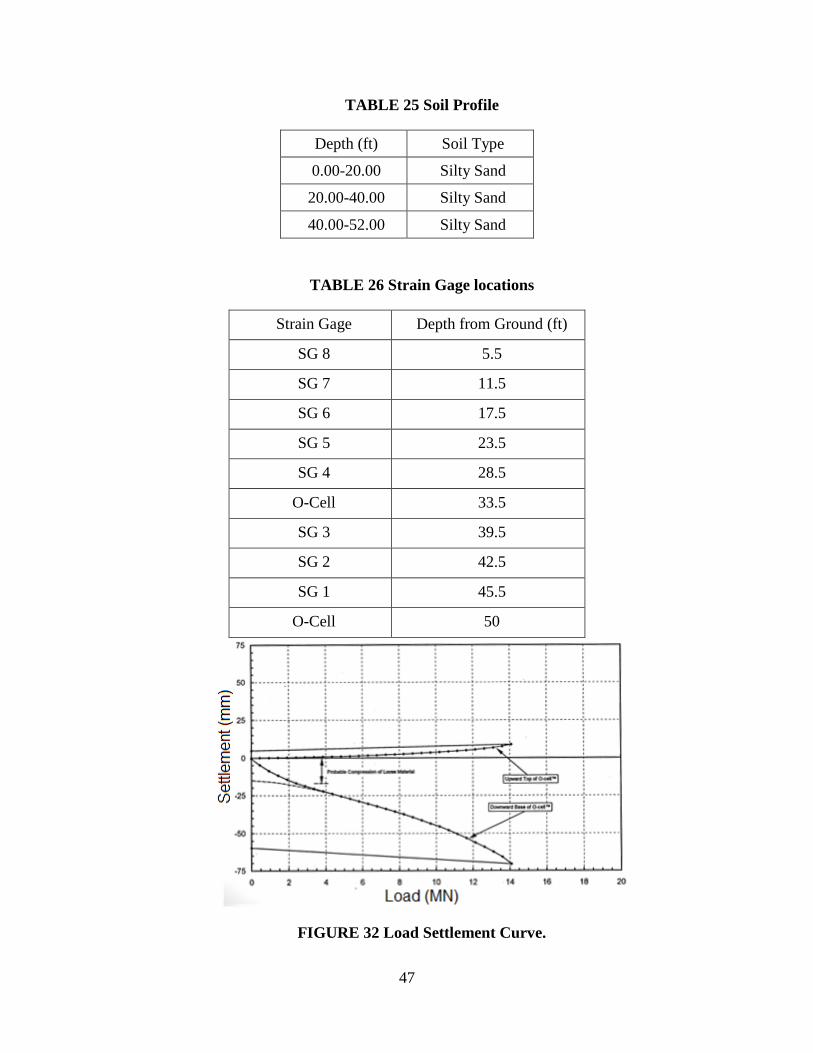
47
TABLE 25 Soil Profile
Depth (ft) Soil Type
0.00-20.00 Silty Sand
20.00-40.00 Silty Sand
40.00-52.00 Silty Sand
TABLE 26 Strain Gage locations
Strain Gage Depth from Ground (ft)
SG 8 5.5
SG 7 11.5
SG 6 17.5
SG 5 23.5
SG 4 28.5
O-Cell 33.5
SG 3 39.5
SG 2 42.5
SG 1 45.5
O-Cell 50
FIGURE 32 Load Settlement Curve.
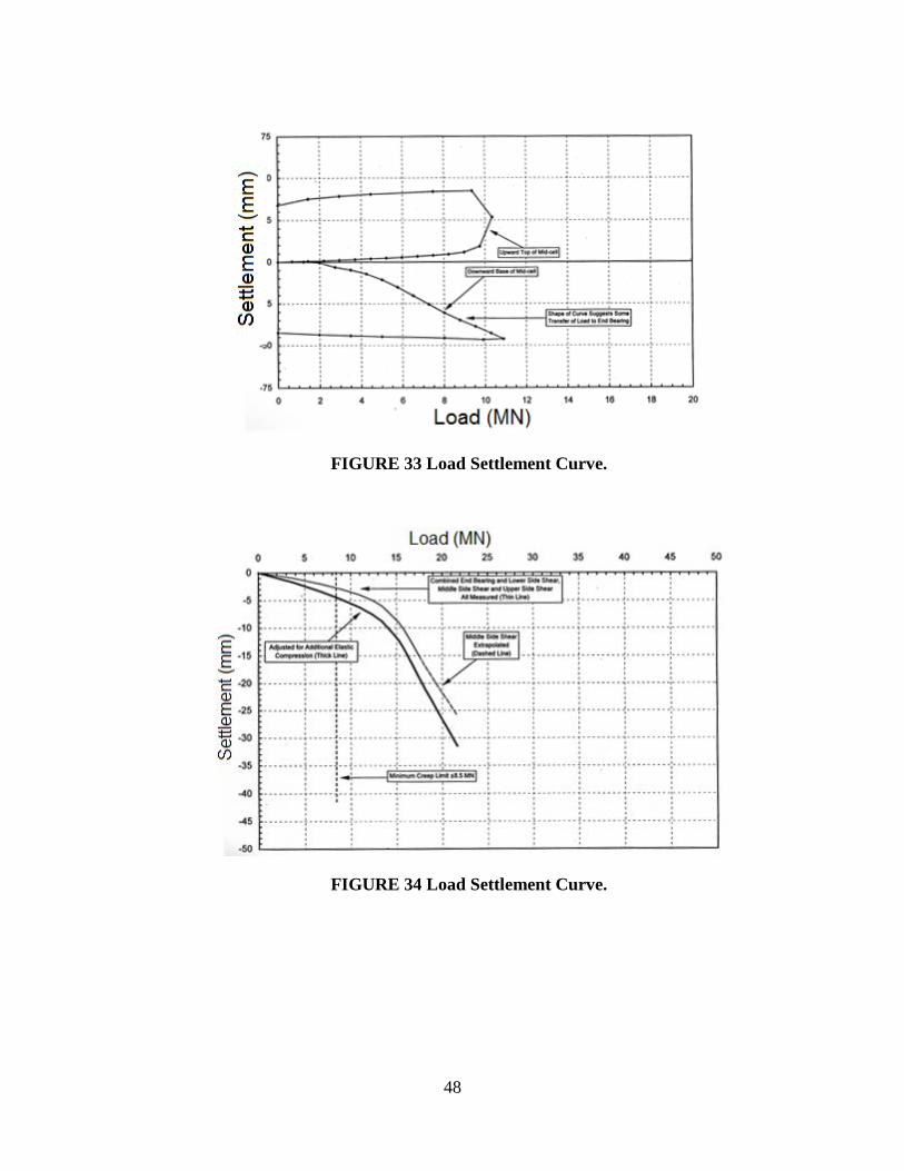
48
FIGURE 33 Load Settlement Curve.
FIGURE 34 Load Settlement Curve.
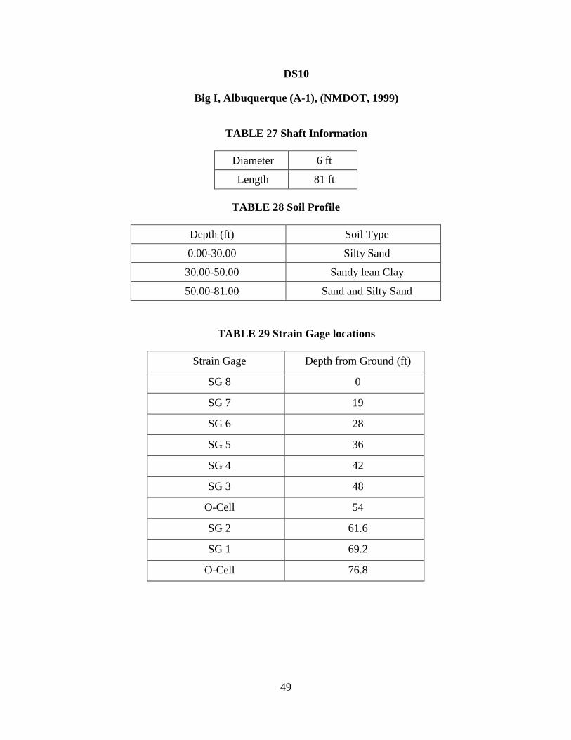
49
DS10
Big I, Albuquerque (A-1), (NMDOT, 1999)
TABLE 27 Shaft Information
Diameter 6 ft
Length 81 ft
TABLE 28 Soil Profile
Depth (ft) Soil Type
0.00-30.00 Silty Sand
30.00-50.00 Sandy lean Clay
50.00-81.00 Sand and Silty Sand
TABLE 29 Strain Gage locations
Strain Gage Depth from Ground (ft)
SG 8 0
SG 7 19
SG 6 28
SG 5 36
SG 4 42
SG 3 48
O-Cell 54
SG 2 61.6
SG 1 69.2
O-Cell 76.8
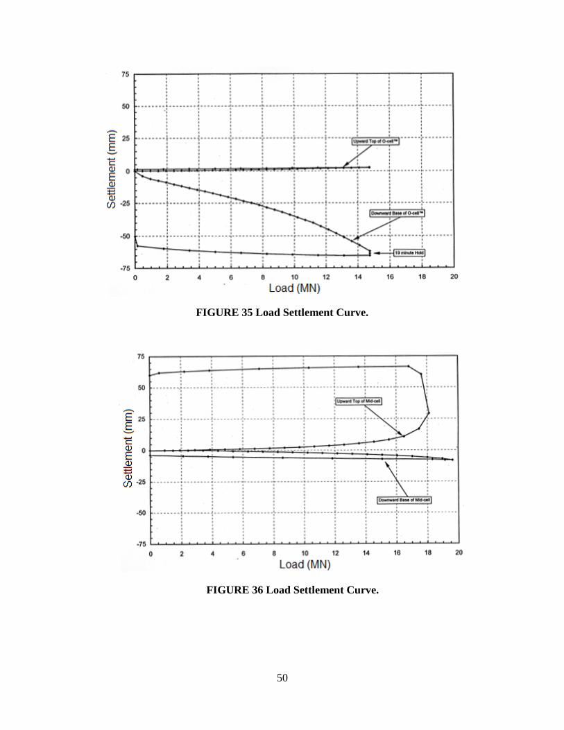
50
FIGURE 35 Load Settlement Curve.
FIGURE 36 Load Settlement Curve.
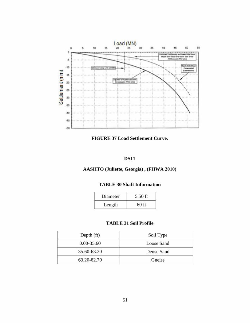
51
FIGURE 37 Load Settlement Curve.
DS11
AASHTO (Juliette, Georgia) , (FHWA 2010)
TABLE 30 Shaft Information
Diameter 5.50 ft
Length 60 ft
TABLE 31 Soil Profile
Depth (ft) Soil Type
0.00-35.60 Loose Sand
35.60-63.20 Dense Sand
63.20-82.70 Gneiss
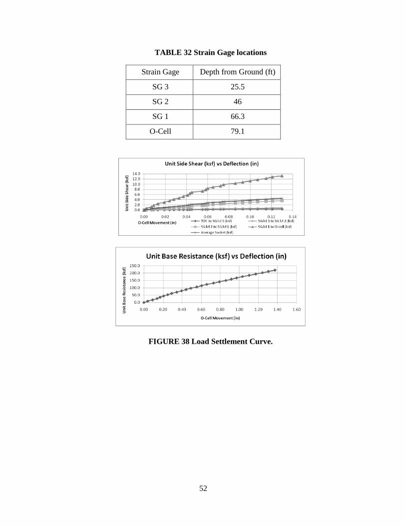
52
TABLE 32 Strain Gage locations
Strain Gage Depth from Ground (ft)
SG 3 25.5
SG 2 46
SG 1 66.3
O-Cell 79.1
FIGURE 38 Load Settlement Curve.

53
DS12 DS13
I-10 (ADOT)-a, (HDR Report, 2010) I-10 (ADOT)-b, (HDR Report, 2010)
TABLE 33 Shaft Information
Diameter 6 ft
Length 115 ft
TABLE 34 Soil Profile
Depth (ft) Soil Type
0.00-8.00 Lean clay
8.00-12.00 Clayey sand
12.00-28.00 Clay w/ sand
28.00-32.00 Clayey sand
32.00-57.00 Silty sand and poorly graded sand
57.00-62.00 Clayey sand
62.00-73.00 Lean clay w/ sand
73.00-77.00 Silty sand
TABLE 35 Strain Gage Locations.
Strain Gage Depth from Ground (ft)
SG 8 28
SG 7 42
SG 6 53
SG 5 63
Mid O-Cell 71
SG 4 79
SG 3 88
SG 2 94
SG 1 103
O-Cell 109
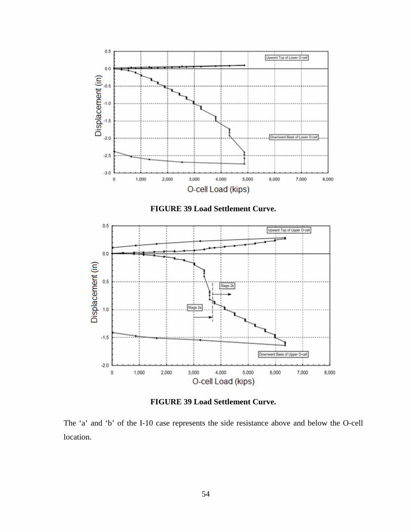
54
FIGURE 39 Load Settlement Curve.
FIGURE 39 Load Settlement Curve.
The ‘a’ and ‘b’ of the I-10 case represents the side resistance above and below the O-cell
location.
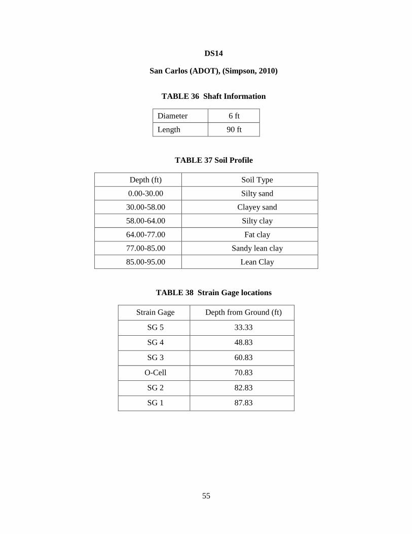
55
DS14
San Carlos (ADOT), (Simpson, 2010)
TABLE 36 Shaft Information
Diameter 6 ft
Length 90 ft
TABLE 37 Soil Profile
Depth (ft) Soil Type
0.00-30.00 Silty sand
30.00-58.00 Clayey sand
58.00-64.00 Silty clay
64.00-77.00 Fat clay
77.00-85.00 Sandy lean clay
85.00-95.00 Lean Clay
TABLE 38 Strain Gage locations
Strain Gage Depth from Ground (ft)
SG 5 33.33
SG 4 48.83
SG 3 60.83
O-Cell 70.83
SG 2 82.83
SG 1 87.83
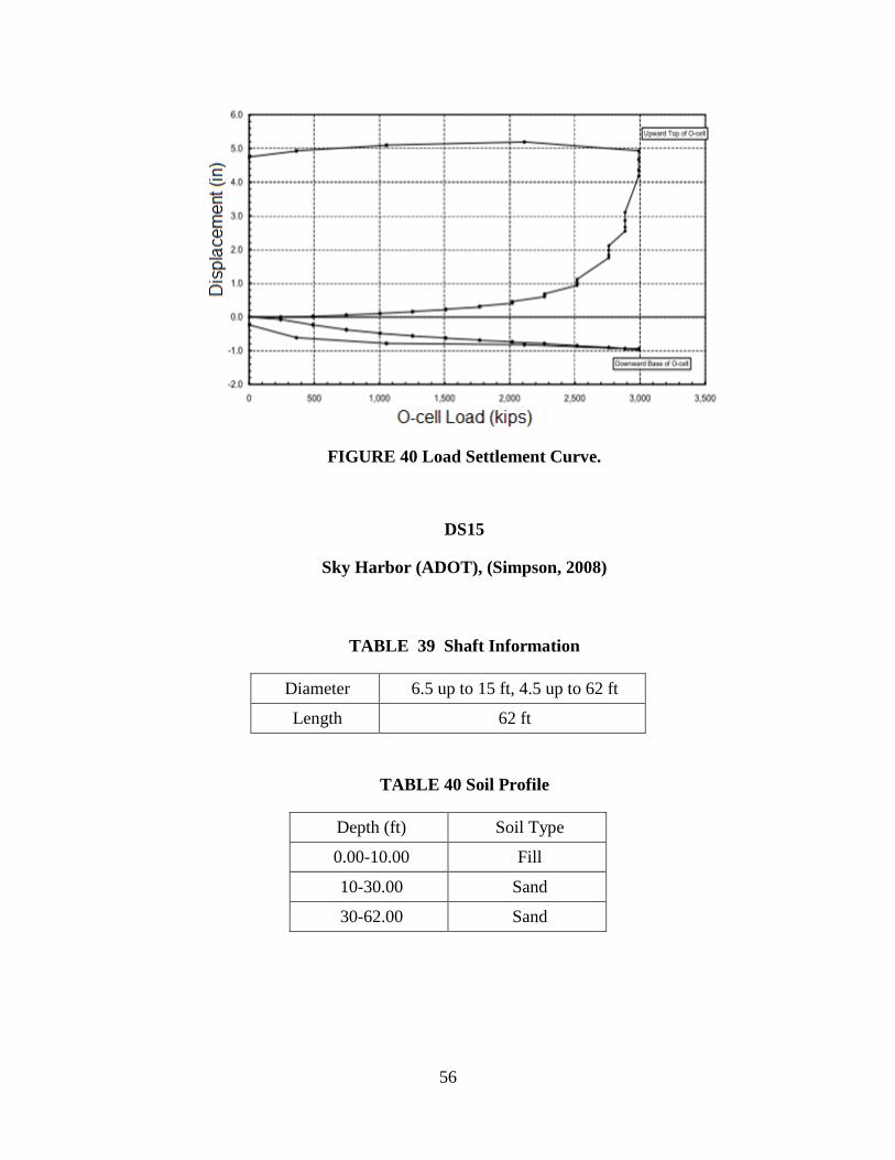
56
FIGURE 40 Load Settlement Curve.
DS15
Sky Harbor (ADOT), (Simpson, 2008)
TABLE 39 Shaft Information
Diameter 6.5 up to 15 ft, 4.5 up to 62 ft
Length 62 ft
TABLE 40 Soil Profile
Depth (ft) Soil Type
0.00-10.00 Fill
10-30.00 Sand
30-62.00 Sand

57
TABLE 41 Strain Gage locations
Strain Gage Depth from Ground (ft)
SG 5 11.93
SG 4 21.93
SG 3 31.93
SG 2 41.93
O-Cell 48.93
SG 1 57.93
FIGURE 41 Load Settlement Curve.
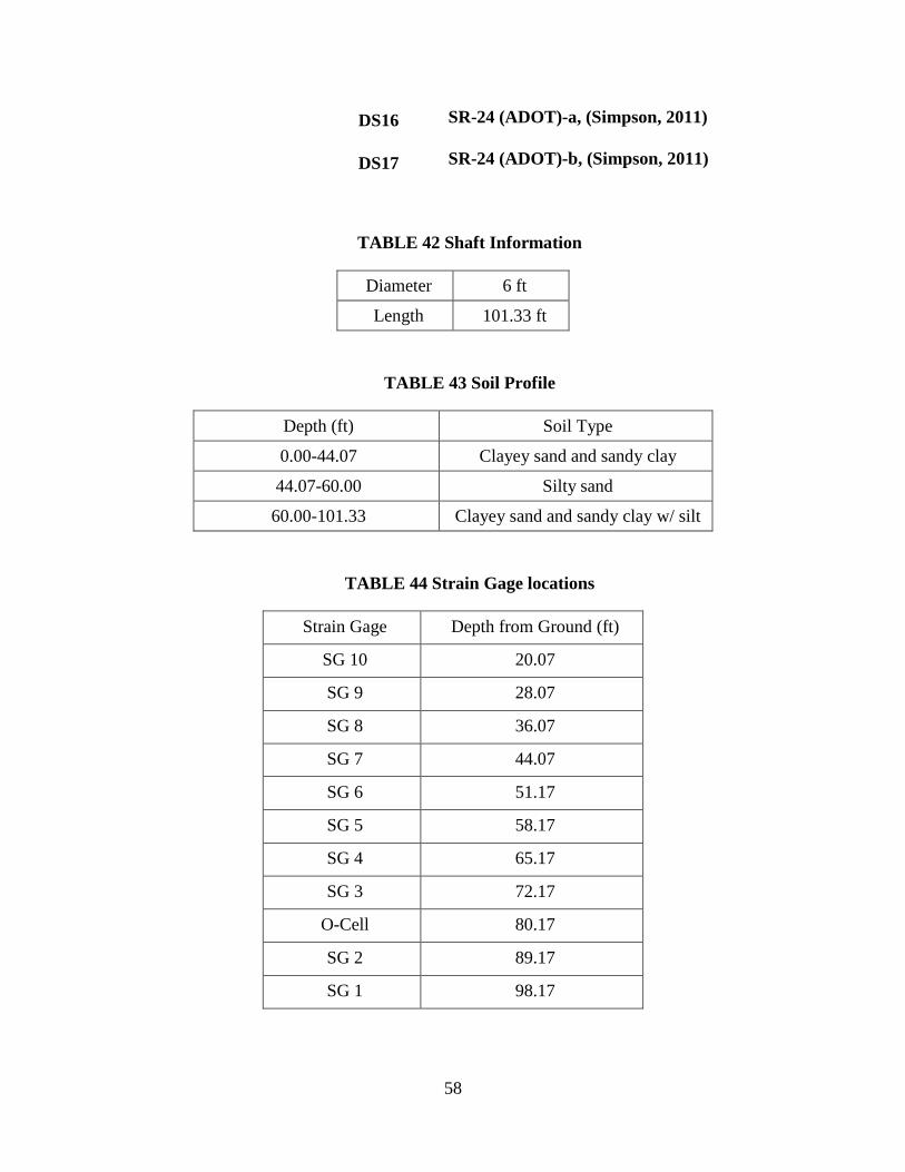
58
DS16 SR-24 (ADOT)-a, (Simpson, 2011)
DS17 SR-24 (ADOT)-b, (Simpson, 2011)
TABLE 42 Shaft Information
Diameter 6 ft
Length 101.33 ft
TABLE 43 Soil Profile
Depth (ft) Soil Type
0.00-44.07 Clayey sand and sandy clay
44.07-60.00 Silty sand
60.00-101.33 Clayey sand and sandy clay w/ silt
TABLE 44 Strain Gage locations
Strain Gage Depth from Ground (ft)
SG 10 20.07
SG 9 28.07
SG 8 36.07
SG 7 44.07
SG 6 51.17
SG 5 58.17
SG 4 65.17
SG 3 72.17
O-Cell 80.17
SG 2 89.17
SG 1 98.17
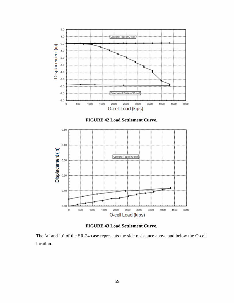
59
FIGURE 42 Load Settlement Curve.
FIGURE 43 Load Settlement Curve.
The ‘a’ and ‘b’ of the SR-24 case represents the side resistance above and below the O-cell
location.

60
DS18
Gila river (ADOT)
TABLE 45 Shaft Information
Diameter 7 ft
Length 117.50 ft
TABLE 46 Soil Profile
Depth (ft) Soil Type
0.00-43.00 Gravel w/ sand
43.00-60.00 Lean clay
60.00-70.00 Silty sand
70.00-75.00 Lean sand
75.00-78.00 Silty sand
78.00-100.00 Fat clay
100.00-115.00 Lean clay
TABLE 47 Strain Gage locations
Strain Gage Depth from Ground (ft)
SG 10 11.29
SG 9 21.29
SG 8 31.29
SG 7 41.29
SG 6 51.29
SG 5 61.29
SG 4 71.29
SG 3 81.04
O-Cell 91.04
SG 2 101.04
SG 1 112.54

61
FIGURE 44 Load Settlement Curve.
DS19
Sunland park (NMDOT), (Simpson, 2006)
TABLE 48 Shaft Information
Diameter 4 ft
Length 74.60 ft
TABLE 49 Soil Profile
Depth (ft) Soil Type
0.00-64.00 Silty sand
64.00-64.70 Silty clay
64.70-74.60 Silty sand
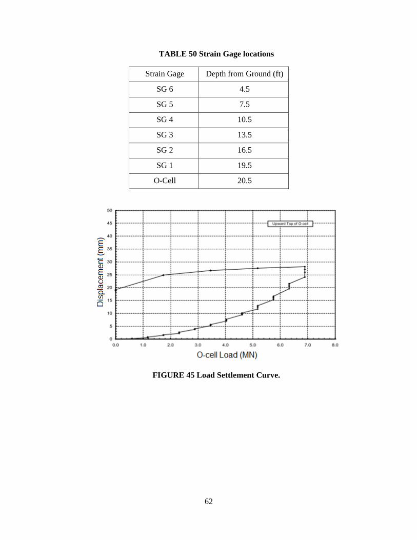
62
TABLE 50 Strain Gage locations
Strain Gage Depth from Ground (ft)
SG 6 4.5
SG 5 7.5
SG 4 10.5
SG 3 13.5
SG 2 16.5
SG 1 19.5
O-Cell 20.5
FIGURE 45 Load Settlement Curve.

63
FIGURE 46 Load Settlement Curve.
DS20
Japan, (Yasufuku & Ochiai, 2006)
TABLE 51 Shaft Information
Diameter 3.94 ft
Length 134.52 ft
No data
TABLE 52 Soil Profile
Depth (ft) Soil Type
0.00-10.00 Silty sand
10.00-85.00 Silty Sand
85.00-115.00 Silty Sand
115.00-134.52 Sand
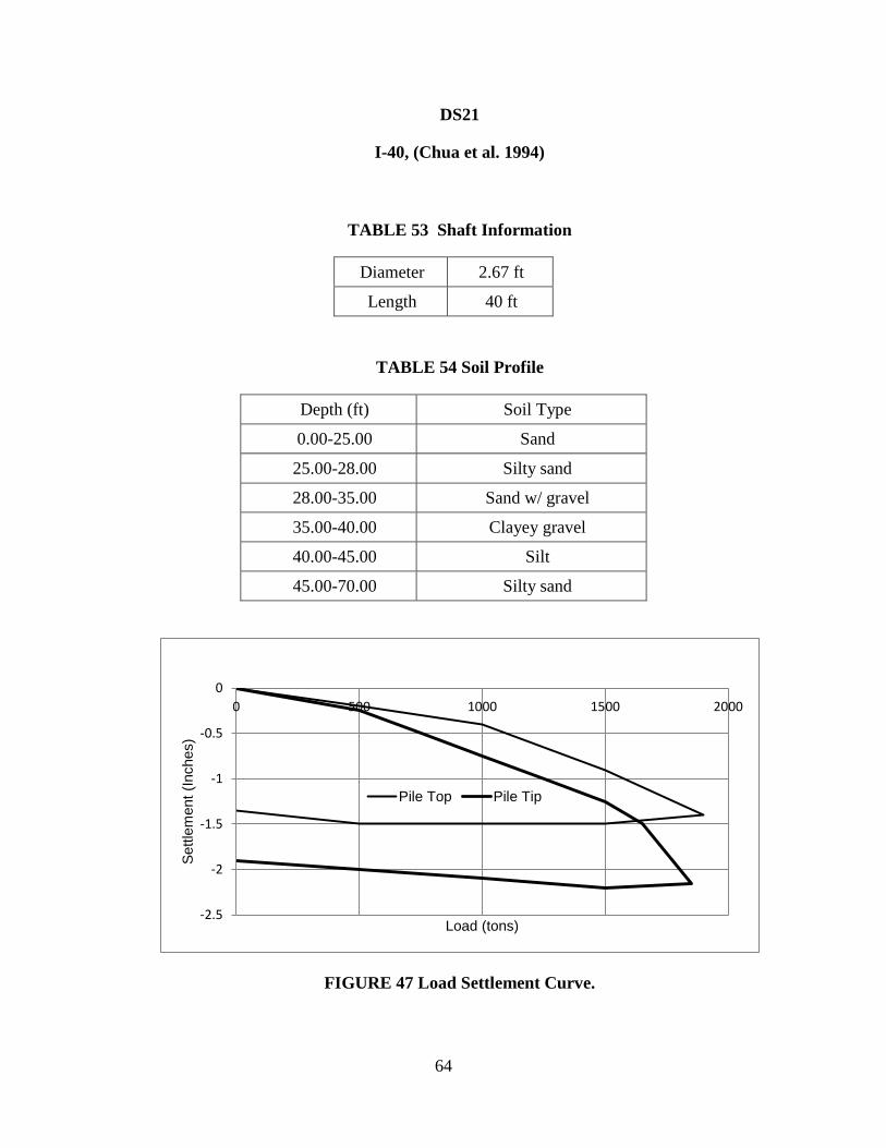
64
DS21
I-40, (Chua et al. 1994)
TABLE 53 Shaft Information
Diameter 2.67 ft
Length 40 ft
TABLE 54 Soil Profile
Depth (ft) Soil Type
0.00-25.00 Sand
25.00-28.00 Silty sand
28.00-35.00 Sand w/ gravel
35.00-40.00 Clayey gravel
40.00-45.00 Silt
45.00-70.00 Silty sand
FIGURE 47 Load Settlement Curve.
-2.5
-2
-1.5
-1
-0.5
00 500 1000 1500 2000
Settl
emen
t (In
ches
)
Load (tons)
Pile Top Pile Tip

65
FIGURE 49 Load Settlement Curve.
00.20.40.60.8
11.21.41.61.8
2
0 50 100 150 200 250 300 350 400
Settl
emen
t (In
ches
)
Load (tons)
Pile Top Pile Tip
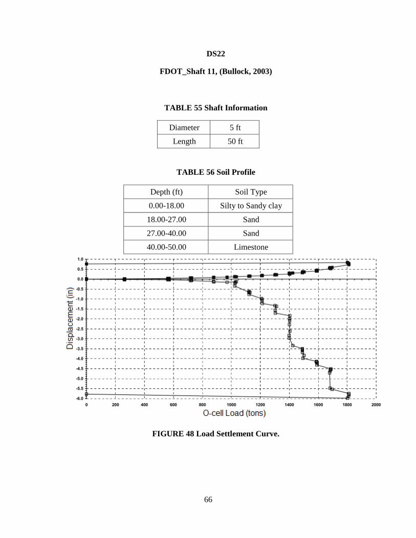
66
DS22
FDOT_Shaft 11, (Bullock, 2003)
TABLE 55 Shaft Information
Diameter 5 ft
Length 50 ft
TABLE 56 Soil Profile
Depth (ft) Soil Type
0.00-18.00 Silty to Sandy clay
18.00-27.00 Sand
27.00-40.00 Sand
40.00-50.00 Limestone
FIGURE 48 Load Settlement Curve.
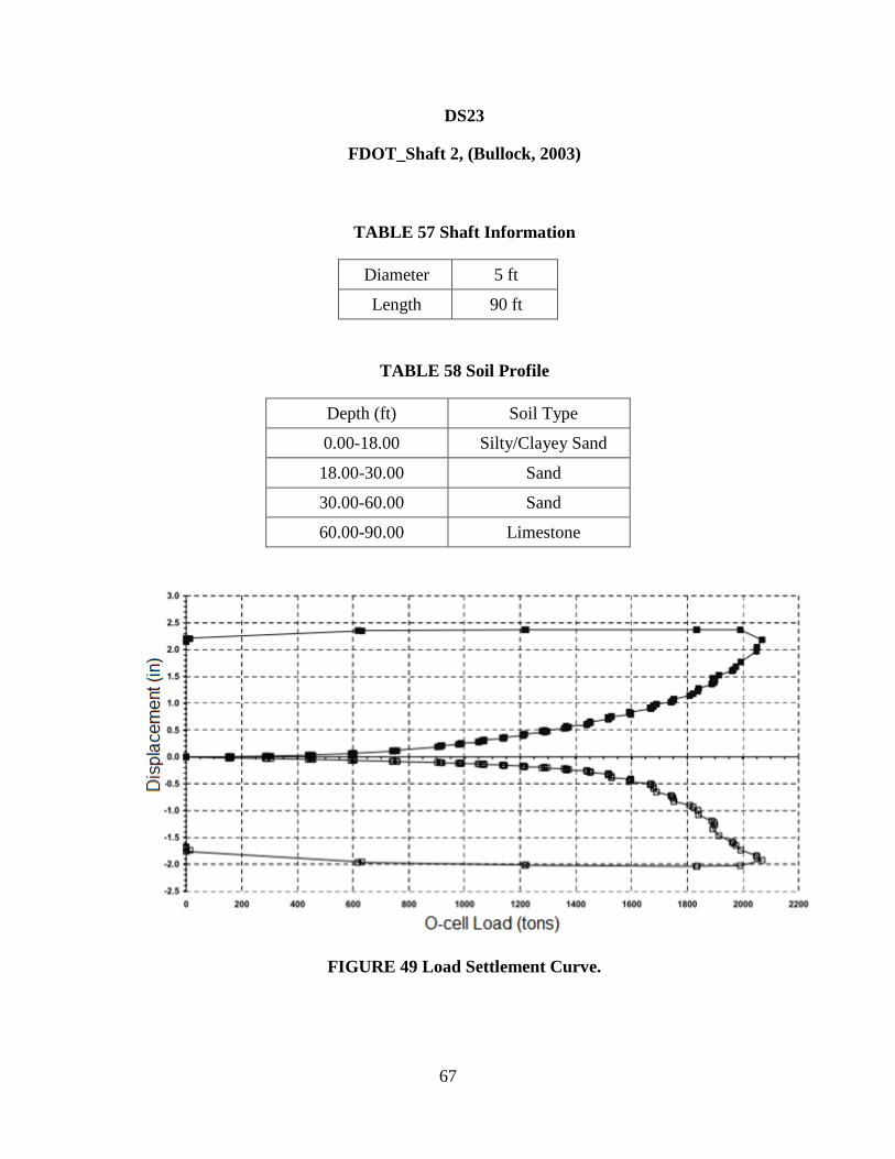
67
DS23
FDOT_Shaft 2, (Bullock, 2003)
TABLE 57 Shaft Information
Diameter 5 ft
Length 90 ft
TABLE 58 Soil Profile
Depth (ft) Soil Type
0.00-18.00 Silty/Clayey Sand
18.00-30.00 Sand
30.00-60.00 Sand
60.00-90.00 Limestone
FIGURE 49 Load Settlement Curve.
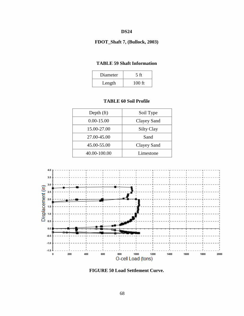
68
DS24
FDOT_Shaft 7, (Bullock, 2003)
TABLE 59 Shaft Information
Diameter 5 ft
Length 100 ft
TABLE 60 Soil Profile
Depth (ft) Soil Type
0.00-15.00 Clayey Sand
15.00-27.00 Silty Clay
27.00-45.00 Sand
45.00-55.00 Clayey Sand
40.00-100.00 Limestone
FIGURE 50 Load Settlement Curve.
69
New Mexico Department of Transportation RESEARCH BUREAU 7500B Pan American Freeway NE PO Box 94690 Albuquerque, NM 87199-4690 Tel: (505) 841-9145

![[AGENCY] CONTRACTS AND PROCUREMENT POLICY AND PROCEDURES ...dot.state.nm.us/content/dam/nmdot/Transit_Rail/ProcurementManual... · [agency] contracts and procurement policy and procedures](https://img.pdfslide.us/doc/110x75/5ae0bbb27f8b9a6e5c8dd48a/agency-contracts-and-procurement-policy-and-procedures-dotstatenmuscontentdamnmdottransitrailprocurementmanualagency.jpg)