Embed Size (px)
Citation preview
c
Development and Evaluation of Fault- tolerant Flight Control Systems
Final Report
(Period Covered: June 15,2000 - December 14,2003)
by Yong D. Song, PhD., P.E.
Department of Electrical Engineering North Carolina A&T State University, Greensboro, NC 27411
NAG4-211
Technical Monitor
Dr. Kajal Gupta
February 27,2004
https://ntrs.nasa.gov/search.jsp?R=20040041407 2018-05-29T20:30:35+00:00Z
I -
t .
NAG4-211
The research is concerned with developing a new approach to enhancing fault tolerance of flight control systems. The original motivation for fault-tolerant control comes from the need for safe operation of control elements (e.g. actuators) in the event of hardware failures in high reliability systems. One such example is modem space vehicle subjected to actuator/sensor impairments. A major task in flight control is to revise the control policy to balance impairment delectability and to achieve sufficient robustness. This involves careful selection of types and parameters of the controllers and the impairment detecting filters used. It also involves a decision, upon the identification of some failures, on whether and how a control reconfiguration should take place in order to maintain a certain system performance level.
In this project new flight dynamic model under uncertain flight conditions is considered, in which the effects of both ramp and jump faults are reflected. Stabilization algorithms based on neural network and adaptive method are derived. The control algorithms are shown to be effective in dealing with uncertain dynamics due to external disturbances and unpredictable faults. The overall strategy is easy to set up and the computation involved is much less as compared with other strategies. Computer simulation software is developed. A serious of simulation studies have been conducted with varying flight conditions.

Table of Contents
Section
summary
Table of Contents
1. Introduction
2. Problem Formulation
3. Neuro-adaptive Fault-tolerant Control
4. Simulation Verification
5. Conclusion and Future Work
6. Acknowledgement
7. References
i
ii
1
1
5
11
16
17
17

1. Introduction
A growing importance has been given in the last few years to the design of a flight
control system able to accomplish the reconfiguration of the aircraft following battle
damage [I]-[5]. While there exists many control methods for flight control, most of the
existing methods are based on "healthy" aircraft model in that the control algorithms are
derived from system dynamics without any faults in the system. Evidently, automatic
control plays a crucial role in achieving these features.
This work is concerned with the development and analysis of neural network based
control algorithms for flight vehicles with faulty dynamics. A neural-adaptive method to
enhance flight vehicle stability under unpredictable faults is presented. The method is
based on the dynamic model coupled with the effect of unpredictable faults and
disturbances. It is shown that with the proposed strategy the effect of faults on the system
performance can be effectively suppressed. The novelty of the proposed approach also
lies in the fact that it is fairly easy to set up and the computation involved is much less as compared with other strategies. An example is used to verify the validity of the proposed
approach.
2. Problem Formulation
The major thrust of this research is directed toward the stabilization of flight vehicle
subject to subsystem failures. The dynamic model considered is of the following form,
M(.)F + N ( i , r ) +d(z) = Bu (1)
with
M ( . ) = M o + p ( t - T f ) M f ( . )
N(.) = No k f l ( t - T f ) N f ( . )
where M E Rm is the inertia matrix depending on the mass property of the vehicle
structure, r~ Rn denotes the coordinatedstates of the system, N E Rnuz represents the
- 1 -

term related to damping and stiffness properties of the system, d e Rn represents the
external disturbance, u E Rm denotes the control signals of the actuator, and BE Rm is
the control input influence matrix reflecting the location of the actuator distributed along
the vehicle structure. In most cases B is a matrix with 0 and 1 as its elements.
The notation " f " is used in the matrices M and N to emphasize the fact that both the
direction and the magnitude of the uncertainties due to modeling approximation and
possible faults are not available for control design.
unknown portion of the dynamics due to a fault occurring at time t 2 Tf . The function
fl(t - Tf ) takes the form
which covers both jump and continuously time-varying (ramp) faults. For the system to
admit a feasible solution under faulty condition, we need to assume that there exists a
positive constant E, >o such that
Tiis assumption implies hat the fault condition under consideration is within atkkabie
range in that it does not dominate the value of A4 under normal conditions. In such a case,
the symmetric and positive definite property of the mass matrix still holds, Le.,
M (.) = M ( . ) T > 0 (2b)
Whenever a fault occurs, system dynamics may be changes in many different ways. In
such a case, our primary objective is to design a proper control to maintain the stability of
the system. Note that essentially two system modes are involved under any fault: critical
modes (denoted by G ) and non-critical modes (denoted by r , ) . The critical modes
should be stabilized explicitly for they are directly related to system safety.
- 2 -
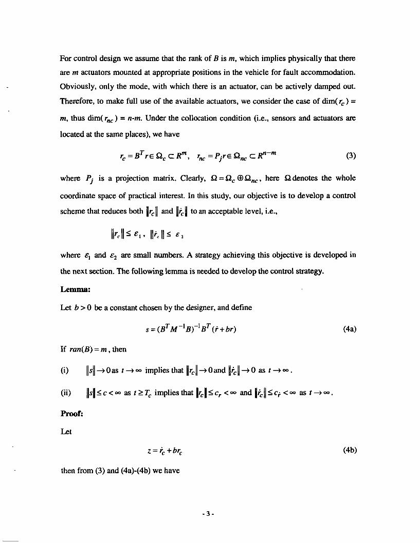
For control design we assume that the rank of B is rn, which implies physically that there
are rn actuators mounted at appropriate positions in the vehicle for fault accommodation.
Obviously, only the mode, with which there is an actuator, can be actively damped out.
Therefore, to make full use of the available actuators, we consider the case of dim( rc ) =
rn, thus dim( rm) = n-rn. Under the collocation condition (i.e., sensors and actuators are
located at the same places), we have
rc = BTrE Q, c Rm, rnc = PjrE Qnc c Rn-m (3)
where Pi is a projection matrix. Clearly, Q = SZ, @QW, here $2 denotes the whole
coordinate space of practical interest. In this study, our objective is to develop a control
scheme that reduces both lrci and Ii,[ to an acceptable level, i.e.,
11% II € 1 ' pc I1 5 E 2
where and
the next section. The following lemma is needed to develop the control strategy.
Lemma:
Let b > 0 be a constant chosen by the designer, and define
are small numbers. A strategy achieving this objective is developed in
(4a) ~ = ( B ~ M - ' B ) -1 B T ( i + b r )
If ran(Bj = rn , then
Proof:
Let
z = i-, + br,
then from (3) and (4a)-(4b) we have
- 3 -
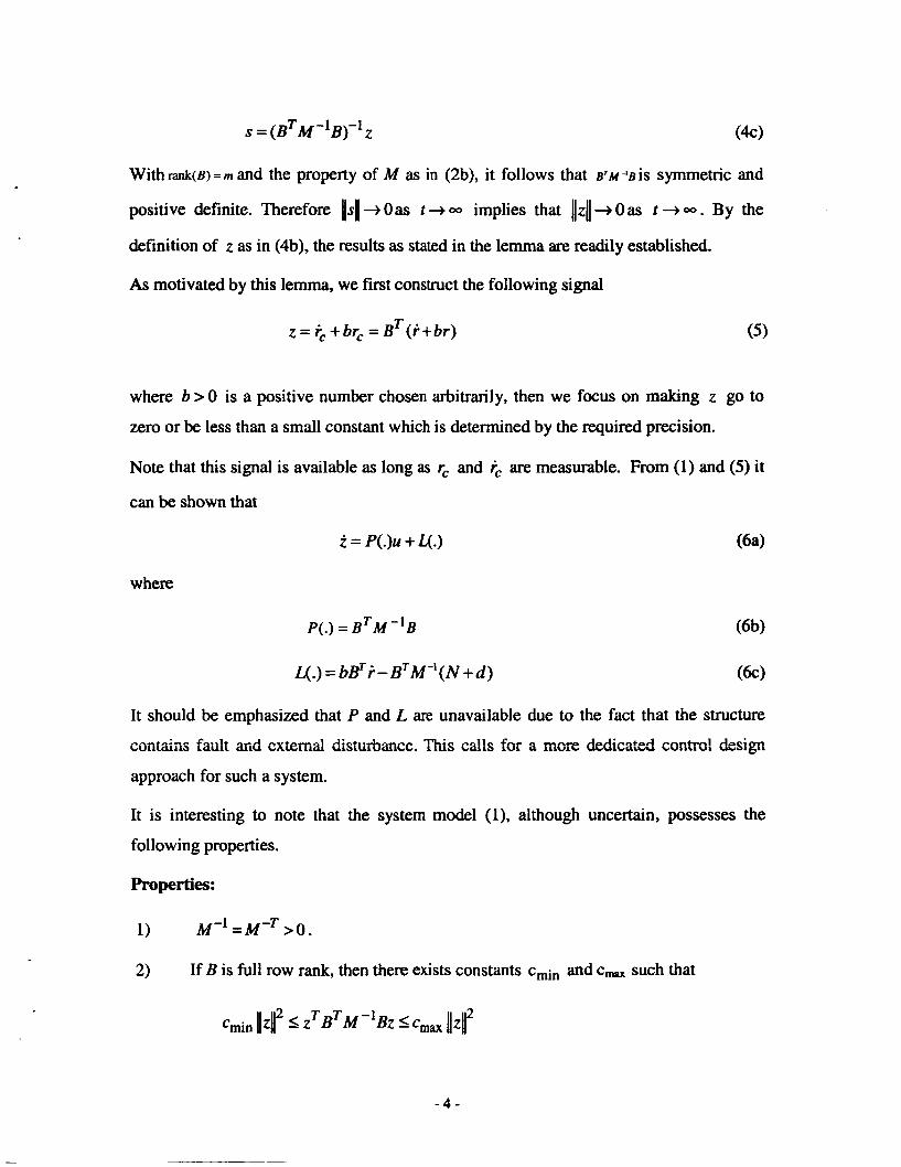
s = (BTM-'B)-'z (k)
With rank(~) = m and the property of M as in (2b), it follows that B ~ M - ~ B ~ S symmetric and
positive definite. Therefore us1 + Oas t + = implies that + Oas c + 0 0 . By the
definition of z as in (4b), the results as stated in the lemma are readily established.
As motivated by this lemma, we first construct the following signal
T z = iC + br, = B (it br) (5)
where b > 0 is a positive number chosen arbitrarily, then we focus on making z go to
zero or be less than a small constant which is determined by the required precision.
Note that this signal is available as long as rc and tC are measurable. From (1) and (5) it
can be shown that
i = P(.)u + L(.) (Gal
where
P(.) = B T M --'B
4.) = bBT i - B7M--' (N + d ) (W
It should be emphasized that P and L are unavailable due to the fact that the structure
zon*&iis fzilt a d zxtcxd &at~~imcc. This cdls f ~ r a ~XGE dedicated control design
approach for such a system.
It is interesting to note that the system model (l), although uncertain, possesses the
following properties.
1) M-' =KT > O .
2) If B is full row rank, then there exists constants cmin and c- such that
- 4 -

T where c- 2 cmin > 0 denotes the maximum and minimum eigenvalues of B M-’B
respectively .
Proof:
The proposition can be easily shown by noting that when B is full row rank BTM-lB is
symmetric and positive definite.
In our later controller design and stability analysis, we only use the fact that such
constants c- and cmax exist, while the actual estimation of these constants is not needed.
To close this section, we re-state the control objective as follows: find a smooth control u
without using the detailed information of P(.) and L(.) such that the system tracking error
vector z locks in a compact set containing origin as time goes by, i.e., lbll I ,u as t > T
(,u is a small constant related to control precision).
3. Neuro-adaptive Fault-tolerant Control
The nonlinear and uncertain nature of P(.) and L(.) represents the major challenge in
control system design. The typical approach is to re-organize L(.) as a linear combination
of some nonlinear functions. This has been the basis for most stable adaptive controllers,
known as the regressor bused method in literature [6]. For complex systems such as
composite structures, this method involves complicated design procedures and heavy
computations. In the early work of neural network based control, a common practice is
to construct multilayer NNs and train these networks via gradient algorithms [7]-[9],
[ 121-[ 131 to approximate P(.) and L(.) respectively. Recognizing the potential instability
associated with these algorithms, several researchers have proposed NN control schemes
using on-line and stable training mechanisms based on Lyapunov stability theory [11]-
WI.
In this work we develop a neuro-adaptive control scheme for the system (1). As a first
step, we “reconstruct” L(.) via the first NN unit as
- 5 -
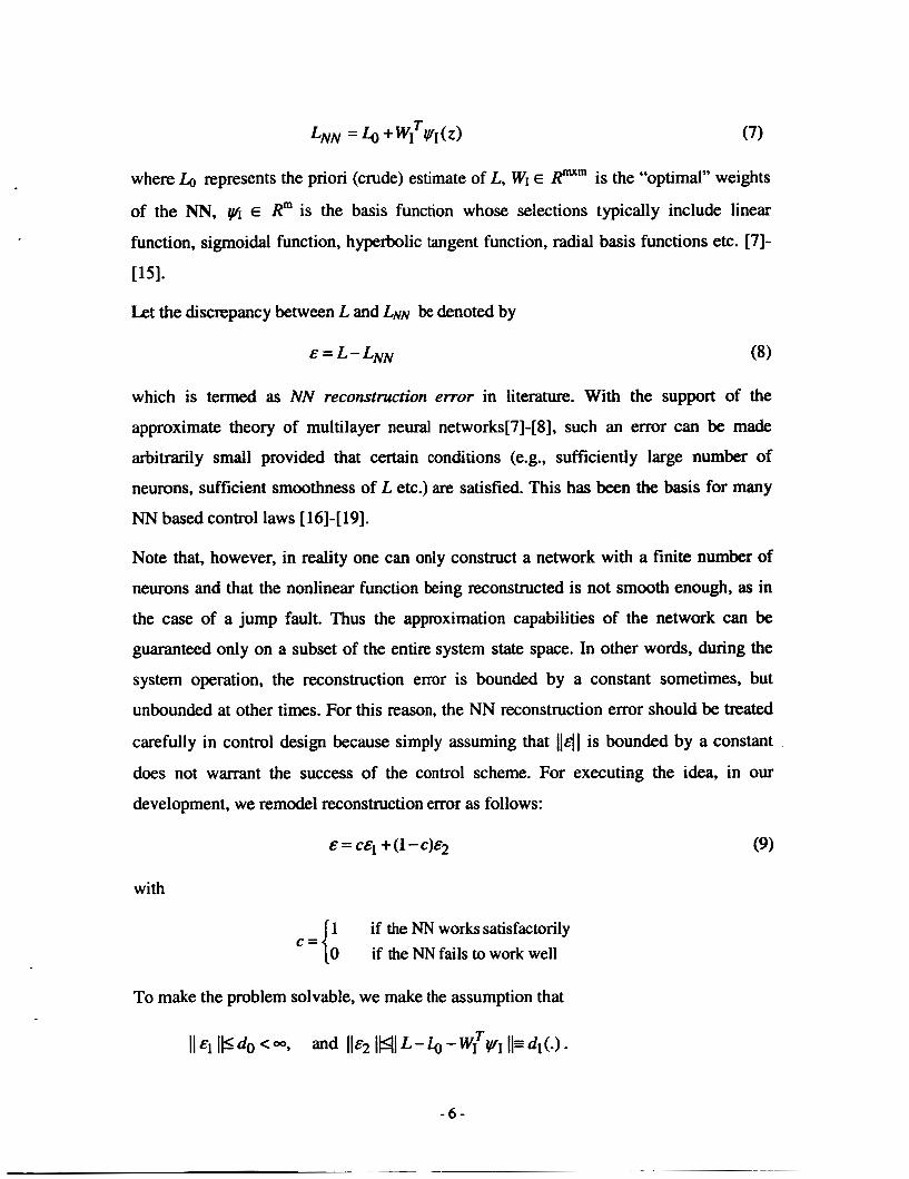
where & represents the priori (crude) estimate of L, WI E Pm is the "optimal" weights
of the NN, pi E R" is the basis function whose selections typically include linear
function, sigmoidal function, hyperbolic tangent function, radial basis functions etc. [7]-
i151.
Let the discrepancy between L and LNN be denoted by
which is termed as NN reconstruction error in literature. With the support of the
approximate theory of multilayer neural networks[7]-[8], such an error can be made
arbitrarily small provided that certain conditions (e.g., sufficiently large number of
neurons, sufficient smoothness of L etc.) are satisfied. This has been the basis for many
NN based control laws [ 161-[ 191.
Note that, however, in reality one can only construct a network with a finite number of
neurons and that the nonlinear function being reconstructed is not smooth enough, as in
the case of a jump fault. Thus the approximation capabilities of the network can be
guaranteed only on a subset of the entire system state space. In other words, during the
system operation, the reconstruction error is bounded by a constant sometimes, but
unbounded at other times. For this reason, the NN reconstruction error should be treated
carefully in control design because simply assuming that 1/41 is bounded by a constant
does not warrant the success of the control scheme. For executing the idea, in our
development, we remodel reconstruction error as follows:
€ = c q +(1-c)€2 (9)
with
1 0
if the NN works satisfactorily if the NN fails to work well
To make the problem solvable, we make the assumption that
II €1 IF do < 0% and llE2 IWI L - r, -WI% II= a . 1 -
- 6 -
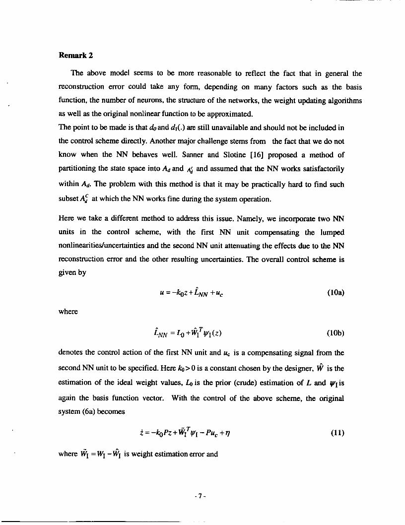
Remark 2
The above model seems to be more reasonable to reflect the fact that in general the
reconstruction error could take any form, depending on many factors such as the basis
function, the number of neurons, the structure of the networks, the weight updating algorithms
as well as the original nonlinear function to be approximated.
The point to be made is that 41 and dl(.) are still unavailable and should not be included in
the control scheme directly. Another major challenge stems from the fact that we do not
know when the NN behaves well. Sanner and Slotine 1161 proposed a method of
partitioning the state space into & and 4 and assumed that the NN works satisfactorily
within &. The problem with this method is that it may be practically hard to find such
subset A: at which the NN works fine during the system operation.
Here we take a different method to address this issue. Namely, we incoprate two NN
units in the control scheme, with the first NN unit compensating the lumped
nonlinearitieduncertainties and the second NN unit attenuating the effects due to the NN
reconstruction error and the other resulting uncertainties. The overall control scheme is
given by
where
(lob)
denotes the control action of the first NN unit and uc is a compensating signal from the
second NN unit to be specified. Here ki~> 0 is a constant chosen by the designer, W is the
estimation of the ideal weight values, Lo is the prior (crude) estimation of L and y ~ i s
again the basis function vector. With the control of the above scheme, the original
system (6a) becomes
i = - b P z + W&I - Pu, + q
where WI = WI - WI is weight estimation error and
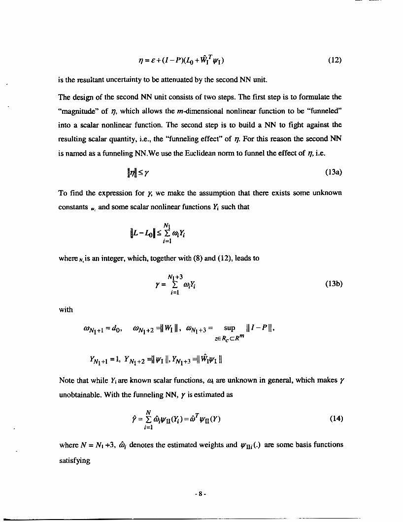
is the resultant uncertainty to be attenuated by the second NN unit.
The design of the second NN unit consists of two steps. The first step is to formulate the
“magnitude” of q, which allows the rn-dimensional nonlinear function to be “funneled”
into a scalar nonlinear function. The second step is to build a NN to fight against the
resulting scalar quantity, i.e., the “funneling effect” of q. For this reason the second NN is named as a funneling “.We use the Euclidean norm to funnel the effect of q, i.e.
To find the expression for x we make the assumption that there exists some unknown
constants and some scalar nonlinear functions yi such that
where N, is an integer, which, together with (8) and (12), leads to
with
Note that while yi are known scalar functions, q are unknown in general, which makes y
unobtainable. With the funneling NN, y is estimated as
where N = Nt +3,
satisfying
denotes the estimated weights and vni(.) are some basis functions
- 8 -
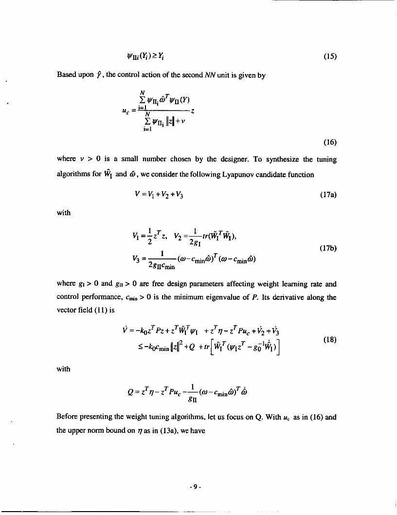
Based upon f , the control action of the second NN unit is given by
(16)
where v > 0 is a small number chosen by the designer. To synthesize the tuning
algorithms for WI and d , we consider the following Lyapunov candidate function
with
1 T 1 - T -
2 %I y=-z z, V2=-tr(W1 WI),
where gI > 0 and gII> 0 are free design parameters affecting weight learning rate and
control performance, c~~ > 0 is the minimum eigenvalue of P. Its derivative along the
vector field (1 1) is
with
Before presenting the weight tuning algorithms, let us focus on Q. With uc as in (16) and
the upper norm bound on 7 as in (13a), we have
- 9 -
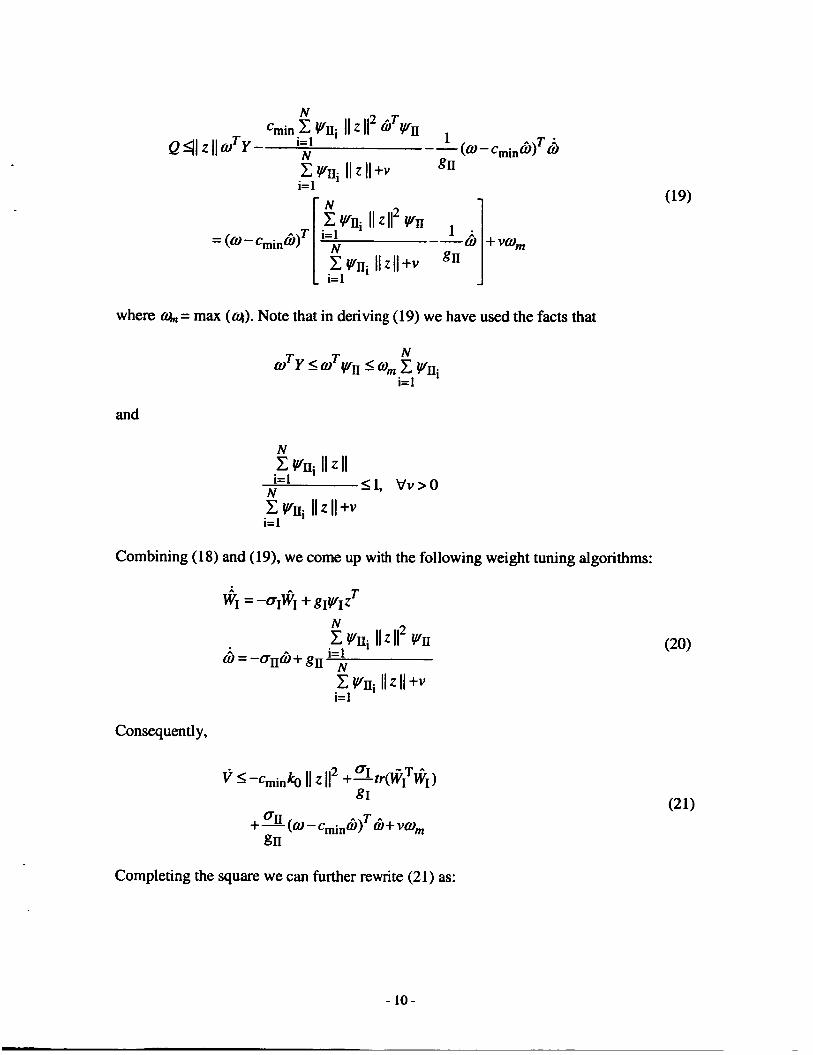
+-(W-CminW) a n A T - w+vwm gn
where & = max (a). Note that in deriving (19) we have used the facts that
N
i= 1
T T w Ylw VnlwmcVf l . 1
and
N c VIIj II z II i= 1 51, vv>o N
Combining (18) and (19), we come up with the following weight tuning algorithms:
Consequently,
Completing the square we can further rewrite (21) as:
- 1 0 -
where
Ai = 2Cdnk(). a2 = bI, A3 = On (23)
are constants independent of z. Note that (22) implies that llzll , ~ I and d are bounded.
Furthermore, from (22), we have
v I -kgcmin 1211' + s
It is seen that v is negative as long as
Therefore, z is confined in the region GI = [ zI llzll I (&)'I. From previous lemma,
we establish that the control error is bounded.
4. Simulation Verification
- 1 1 -
Simulation on a numerical example is conducted to test the effect, deness of the proposed
method. The parameters involved in the algorithms are chosen as
k() =lo, 01 =011 = O S , g1 = g l l = O S , ~ ~ 0 . 0 1 , AT=O.Olsec
The basis functions for the first NN unit are chosen as:

( ~ l i = 0.2, 0.4, ..., XII= . ) 11 where a = 0.5. The basis functions for the second NN unit are selected as in the
following:
where p = 0.5. Ten NN basis functions were used for each of the NN
units: w E RJ , j = 10. All the weights are initialized at zero in the simulation.
As mentioned earlier, any fault due to damage, element malfunction, and so forth, plays
an important role in the behavior of the system. To have a realistic simulation it is
necessary to model the aerodynamic effects of the damage. For this purpose, it may be
said that the changed aircraft dynamics following damages to a stabilator surface is
mainly due to an instantaneous change of the normal force coefficient of the surface, with
the axial force coefficient being usually negligible and with the moment coefficient being
proportional, through the geometry, to the normal force coefficient. Therefore we
consider the expressions for fault in the simulation as follows,
N, (.) = /3 . ( N , i + N , r + N,)
is the fault function, Th=15 sec is the time instant at which the where B=l -e
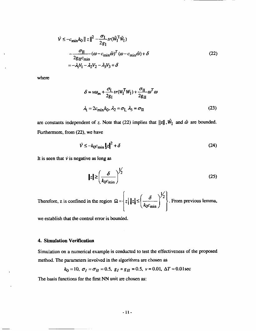
fault occurs, m=0.2 is the fault coefficient. The results are presented in Figures 14,
where Figure 1 is the stabilization error for critical and non-critical modes, Figure 2
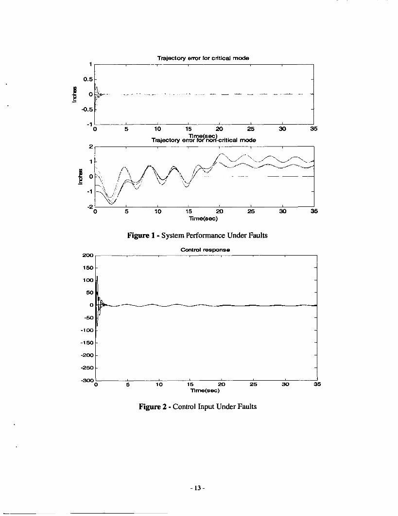
shows the control signals, Figure 3 and Figure 4 illustrated the on-line updating of
weights for the two NN units.
-rn(t-T')
- 12-
Trejectory error for critical mode 1 , I 1
1 5 0
Figure 1 - System Performance Under Faults
-
-50
- 1 0 0
-150
-200
-250
-300
Figure 2 - Control Input Under Faults
- I -
-
-
-
5
- 13-
L

-1 I I I I 1 I I I 0 5 10 15 20 25 30 35
Ti esec Trajectory emr%#ndcritical mode
2 I 1 I r I
1 -
_ _ ~ _ _ _ _ _ _ _ _ _
J
-
-2 I I I I I I
0 5 10 15 20 25 30 35 Time(sec)
1 5 0
1 0 0
501
Figure 1 - System Performance Under Faults
- -
7 -
-
200
- -
-50 -
-100 -
-150 - -
-200 -
-250 -
-300
-
-
-
-
1 I
0 5 10 15 20 25 30
Figure 2 - Control Input Under Faults
35
- 13-
The plot of W 1 hat 0.05
0
-0.05
8 -0.15
-0.2 -
4-25 -
-0.3 ! t
0 5 10 15 20 25 30 35 Time(sec)
Figure 3 - Weights Updating for 1'' Neural Network
t.
0.4
0.2
0 0 5 10 15 20 25 30 35
Xmf3(SeC) -0 5 10 15 20 25 30 35
Xmf3(SeC)
Figure 4 - Weights Updating for 2nd Neural network
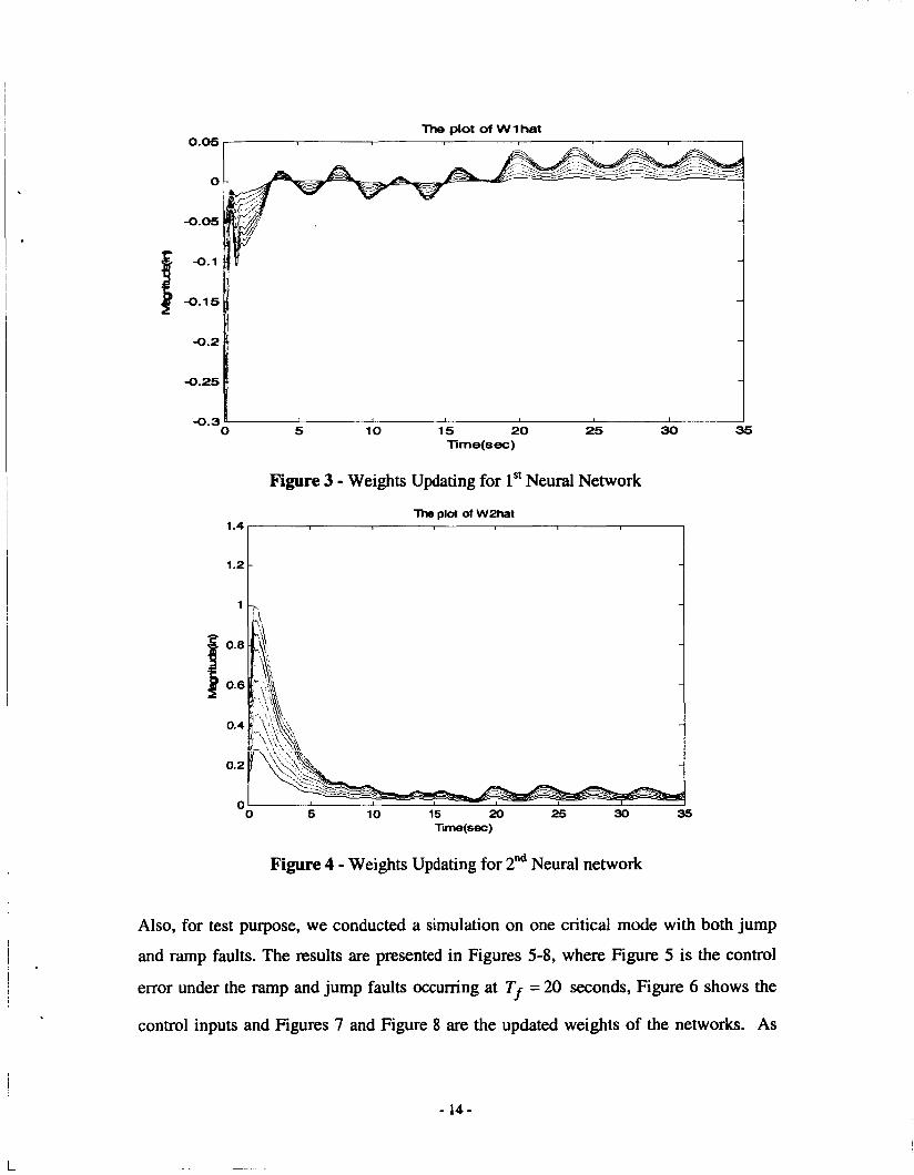
Also, for test purpose, we conducted a simulation on one critical mode with both jump
and ramp faults. The results are presented in Figures 5-8, where Figure 5 is the control
error under the ramp and jump faults occurring at Tf = 20 seconds, Figure 6 shows the
control inputs and Figures 7 and Figure 8 are the updated weights of the networks. As
- 14-

can be seen, with the proposed control method the system remains stable under severe
faults and all the internal signals are bounded and smooth.
I
x ~ -I
z -. I -.- - t o
a .
0 I D 10 *o .O 10 .o 70 .. .o 100 .lm.(.,
.I*
a) ramp fault
o y
-
I . , , . , , , . ,
' 0 * 10 , I 10 1 s 30 .I .o .a
b) jump fault
so
Figure 5 - System Performance Under Faults
2s 14
12 2
IO
I S a
--- I: O S
l 1 2
0 0
a) ramp fault b) jump fault
Figure 7 - Weights Updating for the 1'' Network I
- 15-
.
C r e C n l s U ).. F h t M *.cr(i $ 4 . , , . . , . , ,
a) ramp fault b) jump fault
Figure 8-Weights Updating for the 2nd Network II
5. Conclusion and Future Work Whenever an actuator fault occurs, the element of B is of the form,
where
[aiio f B(t - T')aii (.)I = 0 implies that the actuator is totally failing
Iaii0 f B(t - Tf)aii (.)I = 1 implies the actuation system is health
We are currently investigating the control problem under the following fault conditions,
This, physically, involves a fading actuation fault in which the actuating system has not
totally failed yet. The results will be reported in the forth coming publication.
- 16-
Acknowledgment
The PI would like to thank Dr. Kajal Gupta for his technical support and guidance
throughout this project.
References [l]. L. P. Lyanch. and S. S. Banda, “Active control for vibration damping, ” In S. N.
Atluri and A. K. Amos (Eds.), Springer Series in Computational. Mechanics. New York Springer, 1988,239-261.
[2]. J. Lu, J. S. Thorp and H.-D. Chiang,, “modal control of large flexible space structures using collocated actuators and sensors.”, IEEE Transactions on Automatic Control37, 10, l(1992).
[3]. Iyer, A., and S. N. Singh, “Variable structure slewing control and vibration damping of flexible spacecraft. Acta Astronautica, 25, 1 (1991), 1-9.
[4]. A. Bhaya and C. A. Desor, “On the design of large space structures” IEEE Transaction on Automatic Control, AC-30, 11 1985.
[5]. Y. D. Song and T. Mitchell, “Active Damping Control of Vibrational Systems,” IEEE Trans. On Aerospace and Electronic Svstems, Vol. 32, No. 2,1996, pp. 569-577.
[6]. Y. D. Song, “Adaptive Motion Tracking Control of Robot Manipulators-Non- regressor based Approach,” Int. J. Control, Vol. 63, No. 1, 1996, pp. 41-54.
[7]. K. J. Hunt, D. Sbarbaro, R. Zbikowski, and P. J. Gawthrop, “Neural networks for control systems- a survey,” Automatica ,26, 1085- 11 12,1992.
[SI. W. T. Miller, R. S. Sutton, and P. J. Werbos, Eds, “Neural network for control, 3d.” MlT Press, Cambridge, MA, 1992.
[9j. I(. S . Narendrid and A. M. hrthasarathy, “Identification and Conlroi of Dynamicai Systems Using Neural Networks,” IEEE Trans. on Neural Networks, Vol. 1, No. 1,
“Adaptively Controlling Nonlinear Contiguous-Time Systems Using Multilayer Neural Networks,” ZEEE Trans. on Auto. Control, Vol.
[ 111. F. C. Chen and H. K. Khalil, “Adaptive Control of a Class of Nonlinear Discrete- Time Systems Using Neural Networks,” ZEEE Trans. Auto. Control, Vol. 40, No. 5,
[12].T, Yamada and T. Yabuta, “Neural Network Controller Using Autotuning Method for Nonlinear Functions,” ZEEE Trans. on Neural Networks, Vol. 1, No. 4, July,
[13]. G. Cybenko, “Approximation by Superposition of a Sigmoidal Function,”
1990, pp. 4-27.
[ 101. F. C. Chen and C. C. Liu,
39, NO. 6, 1994, pp. 1306-1310.
1995, pp. 1306-1310.
1992, pp. 595-601.
Mathematics of Control, Signals, and Systems, No. 2, 1989, pp. 303-314.
- 17-
[14].F. L. Lewis, K. Liu and A. Yesildirek, “Neural Net Robot Controller with GuaranteedTracking Performance,” ZEEE Trans. on Neural Networks, Vol. 6,
El51.A. Karakasoglu, S. I. Sudharsanan and M. K. Sundareshan, “Identification and Decentralized Adaptive Control Using Dynamical Neural Networks with Application to Robotic Manipulators,” ZEEE Trans. on Neural Networks, Vol. 4, No. 6, 1993, pp.
[16].R. M. Sanner and J. J. Slotine, “Guassian Networks for Direct Adaptive Control”,
[17].E. Tzirkel-Hancock and F. Fallside, “Stable Control of Nonlinear Systems Using Neural Networks,” Int. J. of Robust and Nonlinear Control, Vol. 2, No. 1, 1992,
[ 181. K. Funahshi, “On the Approximate Realization of Continuous Mappings by Neural Networks,” Neural Networks, Vol. 2, pp. 183-192, 1989.
[ 191. M. Teshnehlab and K. Watanabe, “Self Tuning of Computed Torque Gains by Using Neural Networks with Flexible Structures,” ZEE Proc. -Control Theory Appl., Vol.
NO. 3, 1995, pp. 703-715.
9 19-930.
IEEE Trans. Neural Networks, Vol. 3, No. 6, 1992, pp. 837-863.
pp. 63-85.
141, NO. 4, 1994, pp. 235-242.
-18-