Embed Size (px)
Citation preview
Development and evaluation of a diverse dynamic global
vegetation model based on plant functional tradeoffs
Dissertation
zur Erlangung des Doktorgrades der Naturwissenschaften
im Department Geowissenschaften der Universitat Hamburg
vorgelegt von
Ryan Pavlick
aus Baltimore, Maryland
Hamburg, 2012
Als Dissertation angenommen vom Department Geowissenschaften
der Universitat Hamburg
auf Grund der Gutachten von Prof. Dr. Martin Claussen
und Dr. Axel Kleidon
Hamburg, den 17 Apr 2011
Professor Dr. Jurgen Oßenbrugge
Leiter des Departments fur Geowissenschaften
Abstract
Dynamic Global Vegetation Models (DGVMs) typically abstract the immense diver-
sity of vegetation forms and functioning into a relatively small set of predefined semi-
empirical Plant Functional Types (PFTs). There is growing evidence, however, from
the field ecology community as well as from modelling studies that current PFT schemes
may not adequately represent the observed variations in plant functional traits and their
effect on ecosystem functioning. Also, these PFTs are defined a priori and their simu-
lated distribution is often based on observed relationships between present-day climate
and vegetation patterns. Climate model projections, however, point towards the possi-
bility of regional climates without present-day analogs. This PhD study concerns the
development, evaluation, and application of a novel global vegetation model, the Jena
Diversity-DGVM, which seeks to overcome these deficits with a richer representation
of functional diversity more closely based on first-principles.
JeDi-DGVM simulates the performance of a large number of randomly-generated
plant growth strategies (PGSs), each defined by a set of 15 trait parameters which
characterize various aspects of plant functioning including carbon allocation, ecophys-
iology and phenology. Each trait parameter is involved in one or more functional
tradeoffs. These tradeoffs ultimately determine whether a PGS is able to survive under
the climatic conditions in a given model grid cell and its performance relative to the
other PGSs. The biogeochemical fluxes and land-surface properties of the individual
PGSs are aggregated to the grid cell scale using a mass-based weighting scheme based
on the ‘biomass-ratio hypothesis.
Simulated global biogeochemical and biogeographical patterns are evaluated against
a variety of field and satellite-based observations following a protocol established by
the Carbon-Land Model Intercomparison Project. The land surface fluxes and vegeta-
tion structural properties are reasonably well simulated by JeDi-DGVM, and compare
favorably with other state-of-the-art terrestrial biosphere models. This is despite the
parameters describing the ecophysiological functioning and allometry of JeDi-DGVM
plants evolving as a function of vegetation survival in a given climate, as opposed to
typical approaches that assign land surface parameters for each PFT a priori.
i
Abstract
JeDi-DGVM simulations are run in two configurations to quantify how the repre-
sentation of functional diversity influences the simulated magnitude and variability of
water and carbon fluxes. In the first configuration, we simulate a diverse biosphere
using a large number of plant growth strategies, allowing the modelled ecosystems to
adapt through emergent changes in ecosystem composition. In the second configura-
tion, we recreate a low diversity PFT-like representation of the terrestrial biosphere
by aggregating the surviving growth strategies from the diverse simulation to a sin-
gle community-weighted plant growth strategy per grid cell. In agreement with earlier
biodiversity-ecosystem functioning studies, the diverse representation of terrestrial veg-
etation leads generally to higher productivity and water-use efficiency. The land sur-
face fluxes in the diverse simulations show greater temporal stability and resilience to
climatic perturbations. These results demonstrate a need for improving the represen-
tation of functional diversity in comprehensive Earth System models and add support
for conserving biodiversity to maintain ecosystem services.
The JeDi-DGVM modelling approach developed in this thesis sets the foundation for
future applications, in which the simulated vegetation response to global change has a
greater ability to adapt through changes in ecosystem composition, having potentially
wide-ranging implications for biosphere-atmosphere interactions under global change.
ii
Contents
Abstract i
1 Introduction 1
1.1 Motivation . . . . . . . . . . . . . . . . . . . . . . . . . . . . . . . . . . 1
1.2 Research objectives . . . . . . . . . . . . . . . . . . . . . . . . . . . . . . 3
1.3 Thesis outline . . . . . . . . . . . . . . . . . . . . . . . . . . . . . . . . . 5
2 The Jena Diversity-Dynamic Global Vegetation Model (JeDi-DGVM) 7
2.1 Introduction . . . . . . . . . . . . . . . . . . . . . . . . . . . . . . . . . . 7
2.2 Representation of Trade-offs . . . . . . . . . . . . . . . . . . . . . . . . . 10
2.3 Environmental selection . . . . . . . . . . . . . . . . . . . . . . . . . . . 11
2.4 Aggregation to ecosystem scale . . . . . . . . . . . . . . . . . . . . . . . 12
3 Evaluating the broad-scale patterns of terrestrial biogeography and biogeo-
chemistry 15
3.1 Introduction . . . . . . . . . . . . . . . . . . . . . . . . . . . . . . . . . . 15
3.2 Simulation setup . . . . . . . . . . . . . . . . . . . . . . . . . . . . . . . 15
3.3 Evaluation protocol . . . . . . . . . . . . . . . . . . . . . . . . . . . . . . 16
3.4 Results and discussion . . . . . . . . . . . . . . . . . . . . . . . . . . . . 22
3.4.1 Biodiversity patterns . . . . . . . . . . . . . . . . . . . . . . . . . 22
3.4.2 Phenology . . . . . . . . . . . . . . . . . . . . . . . . . . . . . . . 24
3.4.3 Global carbon stocks . . . . . . . . . . . . . . . . . . . . . . . . . 27
3.4.4 Gross Primary Productivity . . . . . . . . . . . . . . . . . . . . . 27
3.4.5 Net Primary Productivity . . . . . . . . . . . . . . . . . . . . . . 33
3.4.6 Evapotranspiration . . . . . . . . . . . . . . . . . . . . . . . . . . 34
3.4.7 Seasonal cycle of atmospheric CO2 . . . . . . . . . . . . . . . . . 37
3.4.8 Net terrestrial carbon exchange . . . . . . . . . . . . . . . . . . . 39
3.4.9 Comparison with eddy covariance measurements . . . . . . . . . 41
3.4.10 Carbon stocks and flows in Amazonia . . . . . . . . . . . . . . . 42
3.4.11 Sensitivity to elevated atmospheric CO2 . . . . . . . . . . . . . . 43
iii
Contents
3.5 Summary of model evaluation . . . . . . . . . . . . . . . . . . . . . . . . 46
4 Quantifying functional diversity-biospheric functioning relationships 49
4.1 Introduction . . . . . . . . . . . . . . . . . . . . . . . . . . . . . . . . . . 49
4.2 Methods . . . . . . . . . . . . . . . . . . . . . . . . . . . . . . . . . . . . 53
4.2.1 Simulation setup . . . . . . . . . . . . . . . . . . . . . . . . . . . 53
4.2.2 Diversity measures . . . . . . . . . . . . . . . . . . . . . . . . . . 56
4.3 Results . . . . . . . . . . . . . . . . . . . . . . . . . . . . . . . . . . . . . 59
4.3.1 Differences in mean productivity and evapotranspiration . . . . . 59
4.3.2 Differences in variability of productivity and evapotranspiration . 63
4.3.3 Differences in the resilience of the biosphere to climatic perturbation 68
4.4 Discussion . . . . . . . . . . . . . . . . . . . . . . . . . . . . . . . . . . . 76
4.4.1 Diversity-Productivity . . . . . . . . . . . . . . . . . . . . . . . . 76
4.4.2 Diversity-Variability . . . . . . . . . . . . . . . . . . . . . . . . . 77
4.4.3 Diversity-Resilience . . . . . . . . . . . . . . . . . . . . . . . . . 78
4.5 Summary of diversity-biospheric functioning relationships . . . . . . . . 78
5 Summary and outlook 81
5.1 Summary . . . . . . . . . . . . . . . . . . . . . . . . . . . . . . . . . . . 81
5.2 Outlook . . . . . . . . . . . . . . . . . . . . . . . . . . . . . . . . . . . . 82
5.2.1 Representation of tradeoffs . . . . . . . . . . . . . . . . . . . . . 82
5.2.2 Is everything everywhere? . . . . . . . . . . . . . . . . . . . . . . 83
5.2.3 Aggregation scheme and competition . . . . . . . . . . . . . . . . 84
5.2.4 Further evaluation . . . . . . . . . . . . . . . . . . . . . . . . . . 85
5.2.5 Ongoing and potential applications . . . . . . . . . . . . . . . . . 86
A Jena Diversity-Dynamic Global Vegetation (JeDi-DGVM) Model Descrip-
tion 89
A.1 Plant module overview . . . . . . . . . . . . . . . . . . . . . . . . . . . . 89
A.2 Vegetation carbon pool dynamics . . . . . . . . . . . . . . . . . . . . . . 91
A.3 Growing Conditions . . . . . . . . . . . . . . . . . . . . . . . . . . . . . 91
A.4 Germination . . . . . . . . . . . . . . . . . . . . . . . . . . . . . . . . . . 93
A.5 Carbon allocation . . . . . . . . . . . . . . . . . . . . . . . . . . . . . . . 93
A.6 Turnover and Senescence . . . . . . . . . . . . . . . . . . . . . . . . . . . 94
A.7 Land Surface Parameters . . . . . . . . . . . . . . . . . . . . . . . . . . 95
A.8 Net Primary Productivity . . . . . . . . . . . . . . . . . . . . . . . . . . 97
A.9 Scaling from plant growth strategies to community-aggregated fluxes . . 99
A.10 Soil Carbon . . . . . . . . . . . . . . . . . . . . . . . . . . . . . . . . . . 100
iv
Contents
B Land Surface Module 103
B.1 Water storage and runoff generation . . . . . . . . . . . . . . . . . . . . 105
B.2 Potential evapotranspiration . . . . . . . . . . . . . . . . . . . . . . . . . 107
B.3 Actual evapotranspiration . . . . . . . . . . . . . . . . . . . . . . . . . . 108
B.3.1 Sublimation from snow cover . . . . . . . . . . . . . . . . . . . . 108
B.3.2 Evaporation from canopy interception reservoir . . . . . . . . . . 108
B.3.3 Bare soil evaporation . . . . . . . . . . . . . . . . . . . . . . . . . 109
B.3.4 Transpiration . . . . . . . . . . . . . . . . . . . . . . . . . . . . . 109
B.4 Approximation of latent and sensible heat fluxes . . . . . . . . . . . . . 109
C Model parameters and variables 111
Bibliography 119
Acknowledgments 141
v

Chapter 1
Introduction
1.1 Motivation
Human activities are altering the terrestrial biosphere at a large scale and an alarming
rate (Millennium Ecosystem Assessment 2005). The risks associated with these activi-
ties have led to the development of Dynamic Global Vegetation Models (DGVMs; e.g.
Foley et al. 1996; Friend et al. 1997; Woodward et al. 1998; Cox 2001; Sitch et al. 2003).
These mechanistic, process-based, numerical models simulate the large-scale dynamics
of terrestrial ecosystems and have proven useful for testing hypotheses and making
predictions regarding the responses of ecosystem structure and functioning to past
and future environmental changes (see recent review by Quillet et al. 2010). DGVMs
have also been embedded within comprehensive Earth System Models (ESMs) to cap-
ture biogeochemical (e.g. Cox et al. 2000) and biogeophysical (e.g. Foley et al. 2000)
feedbacks between the terrestrial biosphere and the physical climate system. Intercom-
parison studies (Friedlingstein et al. 2006; Sitch et al. 2008), however, have revealed
considerable divergence among the results of these models with respect to the fate of
the terrestrial biosphere and its function as a driver of the global carbon cycle under
projected scenarios of climate change. This divergence may be, at least in part, due
to their coarse and differing treatment of plant functional diversity (Sitch et al. 2008;
Harrison et al. 2010; Fisher et al. 2010b).
For reasons of computational efficiency as well as a lack of sufficient data and theory,
global vegetation models typically represent the immense functional diversity of the
over 300,000 documented plant species to a small number (typically between 4 and
20) of discrete Plant Functional Types (PFTs; Kattge et al. 2011) which are defined a
priori before any simulations are run. In the context of DGVMs, PFTs represent broad
biogeographical, morphological, and phenological aggregations (e.g. tropical broadleaf
evergreen forest or boreal needleleaf deciduous forest) within which parameter values
1
Chapter 1 Introduction
are held spatially and temporally constant and responses to physical and biotic factors
are assumed to be similar (Prentice et al. 2007). They have typically been classified
subjectively using expert knowledge and their occurence within a given model grid
cell is based, either directly or indirectly, on semi-empirical bioclimatic limits, such as
minimum or maximum annual temperature (e.g. Box 1996; Bonan et al. 2002; Sitch
et al. 2003). Inductive approaches have also been proposed wherein PFTs are objec-
tively classified by applying statistical techniques to large datasets of vegetation traits
and climatic variables (e.g. Chapin et al. 1996; Wang and Price 2007). Regardless of
approach, the PFT schemes used by current DGVMs have been criticized as ad hoc
and as ignoring much of our growing knowledge of comparative plant ecology (Harrison
et al. 2010).
In fact, the field ecology community has shown that for many plant traits there is
a large amount of variation within PFTs, and that for several important traits, there
is greater variation within PFTs than between PFTs (Wright et al. 2005; Reich et al.
2007; Kattge et al. 2011). This trait variation may play an important role for many
ecosystem functions (Dıaz and Cabido 2001; Westoby et al. 2002; Ackerly and Cornwell
2007) and for ecosystem resilience to environmental change (Dıaz et al. 2006). Recent
model-data assimilation studies using eddy covariance fluxes (Groenendijk et al. 2011)
as well as other field and satellite-based observations (Alton 2011) provide confirmation
that current PFT schemes are insufficient for representing the full variability of veg-
etation parameters necessary to accurately represent carbon cycle processes. A more
theoretical study by Kleidon et al. (2007) demonstrated that using a small number of
discrete vegetation classes in a coupled climate-vegetation model can lead to potentially
unrealistic multiple steady-states when compared with a more continuous representa-
tion of vegetation. Others have contended that DGVMs may overestimate the negative
effects of climate change by not accounting for potential shifts in ecosystem composi-
tions towards species with traits more suited to the new conditions (Purves and Pacala
2008; Tilman et al. 2006). For example, some coupled climate-vegetation models (e.g.
Cox et al. 2000) project an alarming dieback of the Amazon rainforest under plausible
scenarios of continuing anthropogenic greenhouse gas emissions. The coarse represen-
tation of functional diversity in these models provided by current PFT schemes could
be leading to an overestimation of the strength and abruptness of this response (Fisher
et al. 2010b). Likewise, DGVMs might underestimate the positive effects of environ-
mental changes on ecosystem performance, e.g. by ignoring warm-adapted species in
typically temperature-limited regions (Loehle 1998). Therefore, while PFTs have been
and will likely continue to be useful for many modelling applications, going forward we
2
1.2 Research objectives
will need new approaches that allow for a richer representation of functional diversity
in DGVMs.
Many approaches have been proposed to meet the challenge of improving the repre-
sentation of functional diversity in DGVMs (e.g. Wright et al. 2005; Reich et al. 2007;
Kattge et al. 2009; Harrison et al. 2010). However, so far, most of these continue to
rely on empirical relationships between observed plant traits and environmental (pri-
marily climatic) factors. The utility of such correlational approaches for predicting the
effects of global change on the terrestrial biosphere may be limited, as climate model
projections point towards the possibility of novel climates without modern or paleo
analogs (Jackson and Williams 2004; Williams and Jackson 2007). Other modellers
have introduced schemes in which PFT parameters adapt to environmental conditions;
e.g. with adaptive parameters related to leaf nitrogen (Zaehle and Friend 2010), alloca-
tion (Friedlingstein et al. 1999), and phenology (Scheiter and Higgins 2009). However,
despite some interesting proposals (e.g. Falster et al. 2010; Van Bodegom et al. 2011),
so far no DGVM has sought to mechanistically represent the full range of functional
trait diversity within plant communities (i.e. at the sub-grid scale) using a trait-based
tradeoff approach. Similar approaches have enabled significant progress in modelling
the biogeographical and biogeochemical patterns of global marine ecosystems (Brugge-
man and Kooijman 2007; Litchman et al. 2007; Follows et al. 2007; Dutkiewicz et al.
2009; Follows and Dutkiewicz 2011)
1.2 Research objectives
This thesis introduces a prototype for a new class of vegetation models that mecha-
nistically resolves sub-grid scale trait variability using functional tradeoffs, the Jena
Diversity DGVM (hereafter JeDi-DGVM). Just as the first generation of PFT-based
DGVMs were built upon earlier PFT-based equilibrium biogeography models, JeDi-
DGVM builds upon an equilibrium biogeography model (Kleidon and Mooney 2000,
hereafter KM2000) based on the concept of functional tradeoffs and environmental
filtering. JeDi-DGVM and KM2000 were inspired by the hypothesis ‘Everything is
everywhere, but the environment selects!’ (Baas-Becking 1934; O’Malley 2007). This
nearly century-old idea from marine microbiology postulates that all species (or in the
case of JeDi-DGVM, combinations of trait parameter values) are, at least latently,
present in all places, and that the relative abundances of those species are determined
by the local environment based on selection pressures. Rather than simulating a hand-
3
Chapter 1 Introduction
ful PFTs, JeDi-DGVM simulates the performance of a large number of plant growth
strategies, which are defined by a vector of 15 functional trait parameters. The trait
parameter values determine plant behavior in terms of carbon allocation, ecophysiology,
and phenology and are randomly selected from their complete theoretical or observed
ranges. JeDi-DGVM is constructed such that each trait parameter is involved in one
or more functional trade-offs (Bloom et al. 1985; Smith and Huston 1989; Hall et al.
1992; Westoby and Wright 2006). These tradeoffs ultimately determine which growth
strategies are able to survive under the climatic conditions in a given grid cell as well
as their relative biomasses.
KM2000 demonstrated that this bottom-up plant functional tradeoff approach is ca-
pable of reproducing the broad geographic distribution of plant species richness. More
recently, their approach has provided mechanistic insight into other biogeographical
phenomena including the global patterns of present-day biomes (Reu et al. 2010), com-
munity evenness and relative abundance distributions Kleidon et al. (2009), as well as
possible mechanisms for biome shifts and biodiversity changes under scenarios of global
warming (Reu et al. 2011). JeDi-DGVM extends the KM2000 modelling approach to
a population-based model capable of representing the large-scale dynamics of terres-
trial vegetation and associated biogeochemical fluxes by aggregating the fluxes from
the many individual growth strategies following the ‘biomass-ratio’ hypothesis (Grime
1998).
The major objectives of this study are to:
• To introduce a novel approach to representing functional diversity in a dynamic
global vegetation model, which is less coarse and less reliant on empirical biocli-
matic relationships than previous PFT-based approaches.
• Evaluate if this modelling approach is able to capture the broad-scale present-
day patterns of terrestrial biogeography and biogeochemical fluxes reasonably well
and compare its performance with previous PFT-based models.
• Investigate how a vegetation model with more diverse representation of func-
tional diversity behaves differently relative to a sparse PFT-like representation of
diversity. Specifically, we ask:
– Does a more diverse representation of the terrestrial biosphere lead to gen-
erally higher productivity and evapotranspiration? What modulates the
geographic pattern of these relationship?
– How does the representation of functional diversity influence the temporal
4
1.3 Thesis outline
variability of these biogeochemical fluxes?
– Does a more diverse representation of the terrestrial biosphere lead to greater
resilience of biospheric functioning to large climatic pertubations?
1.3 Thesis outline
The remainder of this thesis is structured as follows:
Chapter 2
The second chapter introduces the novel aspects of the Jena Diversity-Dynamic
Global Vegetation Model (JeDi-DGVM), including how functional diversity has
been implemented via mechanistic trade-offs and how the resulting biogeochemi-
cal fluxes and land-surface properties associated with many plant growth strate-
gies are aggregated to the ecosystem-scale.
Chapter 3
In the third chapter, simulated patterns of terrestrial biogeography and biogeo-
chemistry from JeDi-DGVM are evaluated against a variety of field and satellite-
based observations.The model evaluation follows a systematic protocol established
by the Carbon-Land Model Intercomparison Project (C-LAMP; Randerson et al.
2009). By following this protocol, it is possible to directly compare the bottom-up
functional tradeoff approach of JeDi-DGVM with evaluation results for terrestrial
biosphere models based on the dominant PFT paradigm.
Chapter 4
In the fourth chapter, we use JeDi-DGVM to quantify how differing representa-
tions of functional diversity impact the simulated magnitude and variability of
water and carbon fluxes.
Chapter 5
The fifth chapter begins with a concluding summary of the main findings of this
thesis. We then propose possible directions for further model development and
model evaluation and we highlight a few ongoing and potential applications of
JeDi-DGVM.
Appendices
The appendices contain a detailed description of JeDi-DGVM and the coupled
land–surface scheme.
5

Chapter 1 Introduction
Parts of this thesis are published for 1 open discussion in Biogeosciences Discussions.
1Pavlick, R., Drewry, D. T., Bohn, K., Reu, B., and Kleidon, A.: The Jena Diversity-DynamicGlobal Vegetation Model (JeDi-DGVM): a diverse approach to representing terrestrial biogeographyand biogeochemistry based on plant functional trade-offs, Biogeosciences Discuss., 9, 4627-4726,doi:10.5194/bgd-9-4627-2012, 2012
6
Chapter 2
The Jena Diversity-Dynamic Global
Vegetation Model (JeDi-DGVM)
2.1 Introduction
JeDi-DGVM consists of a plant growth module that is coupled tightly to a land sur-
face module. Both components contain parameterizations of ecophysiological and land
surface processes that are common to many current global vegetation and land sur-
face models. The main novelties in the vegetation component are (i) a mechanistic
representation of functional trade-offs, which (ii) constrain a large number of plant
growth strategies with trait parameter values randomly sampled from their complete
theoretical/observed ranges, and (iii) the aggregation of the fluxes/properties associ-
ated with those growth strategies to grid-scale structure and function based on their
relative abundances. . The following overview of the model focuses on describing the
novel combination of these components and how they are implemented in the model,
while the full description with the detailed parameterizations are described in the Ap-
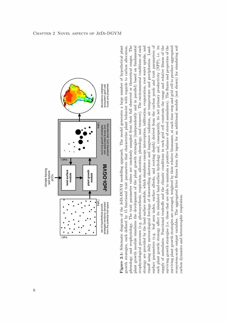
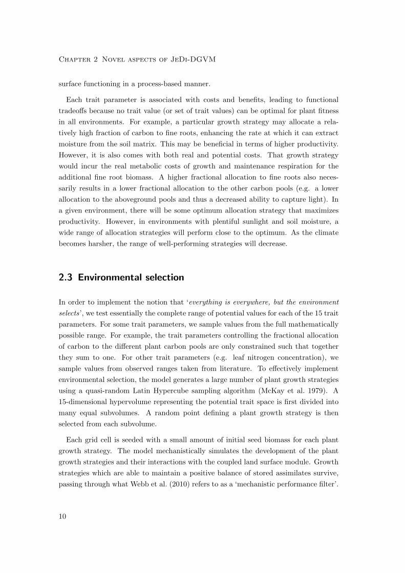
pendices. A schematic diagram of the JeDi-DGVM modelling approach is shown in
Fig. 2.1.
7
Chapter 2 Novel aspects of JeDi-DGVM
plan
t gro
wth
m
odul
e
trait i
trait
j
Fig
ure
10:
(a)
Obse
rvati
on-b
ase
des
tim
ate
of
mea
nannualev
apotr
ansp
irati
on
for
yea
rs1982-
2008
(Jung
etal.,2010);
(b)m
ean
annualgro
sspri
mary
pro
duct
ivity
from
JeD
i-D
GV
Mfo
ryea
rs1982-2
004;and
(c)
the
di↵
eren
cebet
wee
nth
eobse
rvati
on-b
ase
des
tim
ate
and
the
JeD
i-D
GV
Mm
odel
outp
ut.
47
set o
f hyp
othe
tical
gro
wth
st
rate
gies
rand
omly
sam
pled
fro
m th
e po
tent
ial t
rait
spac
e
clim
ate
forc
ing
soil t
extu
repC
O2
land
sur
face
m
odul
e
surv
iving
gro
wth
stra
tegi
es
with
ass
ocia
ted
fluxe
s an
d pr
oper
ties
(incl
. abu
ndan
ces)
abun
danc
e-w
eigh
ted
ecos
yste
m (g
rid-c
ell)
flux
es a
nd p
rope
rties
trait i
trait
j
JeD
i-DG
VM
Figure
2.1:
Sch
emat
icd
iagr
amof
the
JeD
i-D
GV
Mm
od
elli
ng
ap
pro
ach
.T
he
mod
elgen
erate
sa
larg
enu
mb
erof
hyp
oth
etic
al
pla
nt
grow
thst
rate
gies
,ea
chd
efin
edby
15fu
nct
ion
al
trait
para
met
ers
that
chara
cter
ize
pla
nt
beh
avio
rw
ith
regard
sto
carb
on
all
oca
tion
,p
hen
olog
y,an
dec
ophysi
olog
y.T
he
trai
tp
aram
eter
valu
esare
ran
dom
lysa
mp
led
from
thei
rfu
llob
serv
edor
theo
reti
cal
ran
ges
.T
he
pla
nt
grow
thm
od
ule
sim
ula
tes
the
dev
elop
men
tof
the
pla
nt
gro
wth
stra
tegie
s(i
nd
epen
den
tly
an
din
para
llel
)b
ase
don
fun
dam
enta
lec
ophysi
olog
ical
pro
cess
es(e
.g.
ph
otos
ynth
esis
,re
spir
ati
on
,all
oca
tion
,p
hen
olo
gy,
an
dtu
rnov
er).
Th
een
vir
on
men
tal
con
dit
ion
sof
each
stra
tegy
are
pro
vid
edby
the
lan
dsu
rfac
em
od
ule
,w
hic
hsi
mu
late
sca
nopy
inte
rcep
tion
,in
filt
rati
on
,ev
ap
ora
tion
,ro
ot
wate
ru
pta
ke,
an
dru
noff
usi
ng
dai
lym
eteo
rolo
gica
lfo
rcin
gsof
dow
nw
elli
ng
short
wav
ean
dlo
ngw
ave
rad
iati
on
,air
tem
per
atu
rean
dp
reci
pit
ati
on
.L
an
d-
surf
ace
par
amet
ers
(e.g
.le
afar
eain
dex
,su
rface
alb
edo,
an
dro
oti
ng
dep
th)
der
ived
from
the
carb
on
pools
an
dtr
ait
para
met
ers
of
each
pla
nt
grow
thst
rate
gyaff
ect
its
sim
ula
ted
lan
d-s
urf
ace
hyd
rolo
gy
an
d,
con
sequ
entl
y,it
sn
etp
rim
ary
pro
du
ctiv
ity
(NP
P),
i.e.
its
sup
ply
ofas
sim
ilat
es.
Fu
nct
ion
altr
adeo
ffs
and
the
clim
ati
cco
nd
itio
ns
inea
chgri
dce
llco
nst
rain
the
ran
ge
an
dre
lati
vefi
tnes
sof
the
surv
ivin
ggr
owth
stra
tegi
es(i
.e.
thos
eth
atar
eab
leto
main
tain
ap
osi
tive
bala
nce
of
store
dass
imil
ate
s).
Th
efl
uxes
an
dp
rop
erti
esof
the
surv
ivin
gp
lant
grow
thst
rate
gies
are
aver
aged
,w
eighte
dby
thei
rre
lati
ve
bio
mass
es,
at
each
tim
est
epan
dgri
dce
llto
pro
du
ceaggre
gate
dec
osyst
em-s
cale
outp
ut
vari
able
s.T
he
aggr
egate
dli
tter
flu
xes
form
the
inpu
tfo
ran
ad
dit
ion
al
mod
ule
(not
show
n)
for
sim
ula
tin
gso
ilca
rbon
dyn
amic
san
dh
eter
otro
ph
icre
spir
atio
n.
8
2.2 Representation of Trade-offs
2.2 Representation of Trade-offs
When we speak of terrestrial vegetation, we speak of a large number of plants of different
species that differ to some extent in how they grow and respond to the environment.
In fact, in a given environment there are potentially many different strategies by which
individual plant species could grow and cope with the environment, with some ways
being more beneficial to growth and reproductive success than other ways. Some plant
species, for instance, grow and reproduce rapidly, such as grasses, while others, such as
trees, grow slowly and it takes them a long time to reproduce. Some species allocate
a greater proportion of their assimilates to leaves, thereby able to capture more of
the incoming sunlight, while others allocate more to root growth and thereby being
able to access more moisture within the soil. Some species react quickly to a change
in environmental conditions, thereby potentially able to exploit more of the beneficial
conditions for growth, while others are more conservative, thereby potentially avoiding
damage by a turn to less favorable conditions.
To represent this flexibility of how to grow and reproduce in the model, many different
plant growth strategies are simulated simultaneously using the same ecophysiological
parameterizations under the same atmospheric forcing. The only part in which the
plant growth strategies differ is in their values for fifteen functional trait parameters
(Table C.2). These parameters control the amount of carbon from photosynthesis and
storage allocated to six plant carbon pools (allocation), the response times to changes in
environmental conditions and turnover times of the various carbon pools (phenology),
and other aspects of ecophysiological functioning (e.g. leaf nitrogen concentration,
which determines the balance between photosynthesis and respiration).
Each growth strategy is represented by six carbon pools representing leaves, fine
roots, aboveground and belowground wood (stems and coarse roots), storage, and re-
production (‘seeds’). These compartments are linked to the physical functioning of
the land surface in terms of the absorption of solar radiation and soil moisture dy-
namics, which are simulated by the land surface module. For instance, leaf biomass
is linked to the amount of absorbed solar radiation, and fine root biomass to the ca-
pability of a growth strategy to extract soil moisture from the rooting zone. Both of
these examples have functional consequences: more absorbed radiation enhances the
supply of energy for photosynthesis and evapotranspiration, and the amount of ex-
tracted soil water determines the water status of the plant and the supply of moisture
for evapotranspiration. This coupled plant-land surface model is therefore capable of
simulating the interaction between development of a plant growth strategy and land
9
Chapter 2 Novel aspects of JeDi-DGVM
surface functioning in a process-based manner.
Each trait parameter is associated with costs and benefits, leading to functional
tradeoffs because no trait value (or set of trait values) can be optimal for plant fitness
in all environments. For example, a particular growth strategy may allocate a rela-
tively high fraction of carbon to fine roots, enhancing the rate at which it can extract
moisture from the soil matrix. This may be beneficial in terms of higher productivity.
However, it is also comes with both real and potential costs. That growth strategy
would incur the real metabolic costs of growth and maintenance respiration for the
additional fine root biomass. A higher fractional allocation to fine roots also neces-
sarily results in a lower fractional allocation to the other carbon pools (e.g. a lower
allocation to the aboveground pools and thus a decreased ability to capture light). In
a given environment, there will be some optimum allocation strategy that maximizes
productivity. However, in environments with plentiful sunlight and soil moisture, a
wide range of allocation strategies will perform close to the optimum. As the climate
becomes harsher, the range of well-performing strategies will decrease.
2.3 Environmental selection
In order to implement the notion that ‘everything is everywhere, but the environment
selects’, we test essentially the complete range of potential values for each of the 15 trait
parameters. For some trait parameters, we sample values from the full mathematically
possible range. For example, the trait parameters controlling the fractional allocation
of carbon to the different plant carbon pools are only constrained such that together
they sum to one. For other trait parameters (e.g. leaf nitrogen concentration), we
sample values from observed ranges taken from literature. To effectively implement
environmental selection, the model generates a large number of plant growth strategies
using a quasi-random Latin Hypercube sampling algorithm (McKay et al. 1979). A
15-dimensional hypervolume representing the potential trait space is first divided into
many equal subvolumes. A random point defining a plant growth strategy is then
selected from each subvolume.
Each grid cell is seeded with a small amount of initial seed biomass for each plant
growth strategy. The model mechanistically simulates the development of the plant
growth strategies and their interactions with the coupled land surface module. Growth
strategies which are able to maintain a positive balance of stored assimilates survive,
passing through what Webb et al. (2010) refers to as a ‘mechanistic performance filter’.
10
2.4 Aggregation to ecosystem scale
As environmental conditions change, different strategies will respond in different ways,
some may become more productive, others may no longer able to cope with new con-
ditions and die out. Strategies which were previously filtered out will again be given
small amounts of seed carbon and may persist under the new conditions. This process
allows the composition of the plant communities in each grid cell to adapt through
time, without relying on a priori bioclimatic limits relating the presence or absence
of a growth strategy to environmental variables. This mechanistic trial-and-error ap-
proach seems potentially better suited to simulate the response of the biosphere to
climates without present-day analogs because even under new conditions fundamental
functional tradeoffs that all plants face are unlikely to change.
2.4 Aggregation to ecosystem scale
Some mechanism is needed to aggregate the biogeochemical fluxes and vegetation prop-
erties of the potentially many surviving growth strategies within each grid cell. Most
current DGVMs calculate grid-cell fluxes and properties as weighted averages across
fractional coverages of PFTs. Of those models, the competition between PFTs for frac-
tional area in a grid cell is typically computed implicitly based on moving averages of
bioclimatic limits (Arora and Boer 2006). This approach is not suitable for JeDi-DGVM
because its tradeoff-based framework does not rely on a priori bioclimatic limits. A few
DGVMs (e.g. Cox 2001; Arora and Boer 2006) calculate PFT fractional coverages using
a form of the Lotka–Volterra equations, in which the colonization rate of each of N
PFTs is linked through a N -by-N matrix of competition coefficients. For JeDi-DGVM,
this Lotka–Volterra approach quickly becomes computationally burdensome as the size
of the necessary competition matrix increases with the square of the potentially large
number of tested growth strategies. The necessary competition coefficients are also
difficult to determine theoretically (McGill et al. 2006).
Instead, JeDi-DGVM aggregates vegetation fluxes and properties to the grid-cell
scale following the ‘biomass–ratio’ hypothesis (Grime 1998), which postulates that the
immediate effects of the functional traits of a species are closely proportional to the
relative contribution of that species to the total biomass of the community. Recent
work (e.g. Garnier et al. 2004; Vile et al. 2006; Kazakou et al. 2006; Dıaz et al. 2007;
Quetier et al. 2007) supporting the ‘biomass-ratio’ hypothesis has shown strong sta-
tistical links between community-weighted functional traits (i.e. the mean trait values
of all species in a community, weighted by their mass-based relative abundances) and
11
Chapter 2 Novel aspects of JeDi-DGVM
observed ecosystem functions (e.g. aboveground net primary productivity and litter
decomposition). Others have combined the concept of community-weighted functional
traits with the Maximum Entropy (MaxEnt) formalism from statistical mechanics to
successfully make predictions, in the other direction, about the relative abundances of
individual species within communities (e.g. Shipley et al. 2006b; Sonnier et al. 2010;
Laughlin et al. 2011).
Here, rather than weighting the functional traits, JeDi-DGVM calculates ecosystem-
scale variables by directly averaging the fluxes and properties across all surviving growth
strategies, weighting the contribution of each strategy by its current biomass relative
to the total biomass of all strategies within that grid cell (see Appendix A.9 for more
details). The resulting ecosystem-scale variables are for the most part diagnostic and do
not influence the development of the individual growth strategies or their environmen-
tal conditions. Although, the community-aggregated litter fluxes do form the input for
a relatively simple soil carbon module, which then provides simulated estimates of het-
erotrophic respiration (see Appendix A.10). This implementation of the ‘biomass-ratio’
hypothesis assumes that interactions between plants, both competitive and facilitative,
are weak and do not significantly alter plant survival or relative fitness. The potential
implications of this assumption are discussed in Chapter 5.2.3. In principle, the trait
parameters of the surviving growth strategies could also be aggregated, forming an
additional testable output of the model. This is discussed further in Chapter 5.2.4.
12

Chapter 3
Evaluating the broad-scale patterns of
terrestrial biogeography and
biogeochemistry
3.1 Introduction
In this chapter, simulated patterns of terrestrial biogeography and biogeochemistry
from JeDi-DGVM are evaluated against a variety of field and satellite-based observa-
tions. The model evaluation follows a systematic protocol established by the Carbon-
Land Model Intercomparison Project (C-LAMP; Randerson et al. 2009). By following
this protocol, we are also able to directly compare the bottom-up functional trade-off
approach of JeDi-DGVM with evaluation results for terrestrial biosphere models based
on the dominant PFT paradigm. We also evaluate the simulated biogeographical pat-
terns of functional richness and relative abundances to illustrate the parsimonious na-
ture of a functional trade-off approach to dynamic global vegetation modelling, i.e. it
can provide more types of testable outputs with fewer inputs.
3.2 Simulation setup
In our simulation setup, we followed the experimental protocol from C-LAMP (Rander-
son et al. 2009) to facilitate comparison with other terrestrial biogeochemistry models.
JeDi-DGVM was run with 2000 randomly-sampled plant growth strategies on a global
grid at a spatial resolution of approximately 2.8◦ by 2.8◦ resolution, covering all land
areas except Antarctica. The model was forced at a daily time step with downward
shortwave and longwave radiation, precipitation, and near-surface air temperature from
13
Chapter 3 JeDi-DGVM overview and evaluation
an improved NCEP/NCAR atmospheric reanalysis dataset (Qian et al. 2006). We
looped the first 25 years of the reanalysis dataset (1948-1972) with a fixed, preindus-
trial atmospheric CO2 concentration until the vegetation and soil carbon pools reached
a quasi-steady state (∼3500 years). After this spinup simulation, a transient simulation
was run for years 1798-2004 using prescribed global atmospheric CO2 concentrations
from the C4MIP reconstruction of Friedlingstein et al. (2006). This transient simula-
tion was forced by the same climate forcing as the spinup run for years 1798-1947 and
by the full reanalysis dataset for years 1948-2004. We ran an additional experiment to
compare the response of JeDi-DGVM to a sudden increase in atmospheric CO2 with re-
sults from the Free-Air CO2 Enrichment (FACE) experiments (Norby et al. 2005). This
FACE experiment simulation was similar to the transient simulation described above
but with the atmospheric CO2 concentration set to 550 ppm for years 1997-2004. We
deviated from the C-LAMP experimental protocol by allowing the vegetation to evolve
dynamically through the simulations, rather than prescribing the pre-industrial land
cover dataset. The aspects of the C-LAMP protocol related to N deposition were not
considered as a nitrogen cycle has not yet been implemented in JeDi-DGVM.
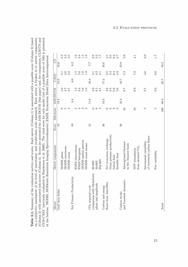
3.3 Evaluation protocol
We evaluated the performance of the JeDi-DGVM against multiple observational datasets
using a set of systematic metrics developed for the C-LAMP (Randerson et al. 2009).
As computed, each C-LAMP metric falls somewhere between zero and one and is then
scaled by a numerical weight to produce a score. The weights are based on subjec-
tive estimates of a metric’s uncertainty, considering both the measurement precision of
the observations and the scaling mismatch between the model and observations. Fur-
ther details about each metric and the justifications behind their particular numerical
weighting are described in Randerson et al. (2009). The metrics, their weights, along
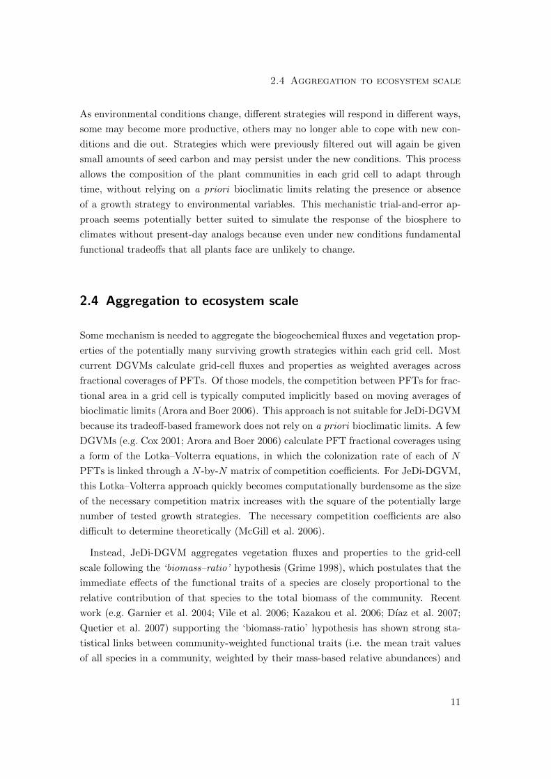
with the resulting scores for JeDi-DGVM are summarized in Table 3.1. The scores for
two terrestrial biogeochemistry models based on the PFT concept, CLM-CN (Thornton
et al. 2007) and CLM-CASA’ (Fung et al. 2005; Doney et al. 2006), are also shown for
comparison (both were previously evaluated in Randerson et al. 2009). Below, we pro-
vide a brief summary of the datasets and scoring methods. The results of the evaluation
are described in the following section.
14
3.3 Evaluation protocolTable
3.1:
Su
mm
ary
of
the
eval
uat
ion
met
rics
an
dsc
ore
s.E
ach
met
ric
(Colu
mn
1)
isass
oci
ate
dw
ith
ap
oss
ible
score
(Colu
mn
3)
base
don
asu
bje
ctiv
eas
sess
men
tof
its
leve
lof
un
cert
ain
tyan
dm
od
el-d
ata
scale
mis
matc
h.
Each
met
ric
isb
roke
nin
tom
etri
cco
mp
on
ents
(Col
um
n2)
wit
has
soci
ated
sub
-sco
res
(Col
um
n4).
Sco
res
are
pre
sente
dfo
rJeD
i-D
GV
M(t
his
pap
er)
an
d,
for
com
pari
son
,C
LM
-CN
an
dC
LM
-CA
SA
’(p
revio
uly
eval
uat
edin
Ran
der
son
etal.
2009).
Th
eto
tal
score
for
each
mod
el(o
ut
of
ap
oss
ible
score
of
100)
ispre
sente
dat
the
bot
tom
.M
OD
IS,
MO
Der
ate
Res
olu
tion
Imagin
gS
pec
trora
dio
met
er;
EM
DI,
Eco
syst
emM
od
elD
ata
Inte
rcom
pari
son
Met
ric
Met
ric
com
ponen
tsSco
reSub-s
core
JeD
i-D
GV
MC
ASA
’C
N
Lea
fA
rea
Index
15
13.4
13.5
12.0
MO
DIS
phase
65.0
5.1
4.2
MO
DIS
maxim
um
54.7
4.6
4.3
MO
DIS
mea
n4
3.7
3.8
3.5
Net
Pri
mary
Pro
duct
ivit
y10
8.4
8.0
8.2
EM
DI
obse
rvati
ons
21.5
1.5
1.6
EM
DI
his
togra
m4
3.4
3.0
3.4
MO
DIS
spati
al
patt
ern
21.6
1.6
1.4
MO
DIS
zonal
mea
ns
21.9
1.9
1.8
CO
2se
aso
nal
cycl
e15
11.8
10.4
7.7
com
pari
son
wit
hG
lobalv
iew
60-9
0N
64.9
4.1
2.8
phase
and
am
plitu
de
30-6
0N
64.5
4.2
3.2
EQ
-30N
32.5
2.1
1.7
Carb
on
and
ener
gy
30
18.3
17.2
16.6
fluxes
from
Am
erifl
ux
Net
ecosy
stem
exch
ange
62.6
2.5
2.1
Gro
sspri
mary
pro
duct
ivit
y6
3.5
3.4
3.5
Late
nt
hea
t9
6.6
6.4
6.4
Sen
sible
hea
t9
5.6
4.9
4.7
Carb
on
stock
s30
16.3
16.7
13.8
and
transi
ent
dynam
ics
Ab
oveg
round
bio
mass
10
6.7
5.3
5.0
inth
eA
mazo
nbasi
n
NP
Pst
imula
tion
10
6.9
7.9
4.1
from
elev
ate
dC
O2
Inte
rannual
vari
abilit
y5
2.7
3.6
3.0
of
terr
estr
ial
carb
on
fluxes
Fir
eva
riabilit
y5
0.0
0.0
1.7
Tota
l100
68.2
65.7
58.4
15
Chapter 3 JeDi-DGVM overview and evaluation
Phenology
We compared the simulated leaf area index (LAI) values against observations from
the MODerate resolution Imaging Spectroradiometer (MODIS) (Myneni et al. 2002;
Zhao et al. 2005, MOD15A2 Collection 4). We consider three phenology metrics, the
timing of maximum LAI, the maximum monthly LAI, and the annual mean LAI. All
three metrics used monthly mean LAI observations and modelled estimates from years
2000 to 2004. The LAI phase metric was computed at each grid cell as the offset
in months between the observed and simulated maximum LAI values, normalized by
the maximum possible offset (6 months), and finally, averaged across biomes. The
maximum and annual mean LAI metrics M were computed using the equation:
M = 1−
n∑i=1
|mi−oi|mi+oi
n(3.1)
where mi is the simulated LAI at the grid cell corresponding to the satellite observation
(oi) and n is the number of model grid cells in each biome. Global means for these
metrics were computed by averaging M across different biome types.
Global patterns of productivity and evapotranspiration
Modelled estimates of net primary productivity (NPP) are compared against a com-
pilation of field-based observations from the Ecosystem Model Data Intercomparison
(EMDI) (Olson et al. 2001) and remote sensing-based estimates extracted from the
MODIS MOD17A3 Collection 4.5 product (Heinsch et al. 2006; Zhao et al. 2005, 2006).
We compared the mean annual NPP as simulated by JeDi-DGVM for years 1975-2000
with the EMDI observations on a point-by-point basis of each observation site to the
corresponding model grid cell using Eq. 3.1 described above. As a second NPP metric,
we used Eq. 3.1 again with the modeled and observed values averaged into discrete
precipitation bins of 400mm per year. For the third and fourth NPP metrics, we com-
puted the square of the Pearson coefficient of determination (r2) between the mean
annual MODIS and modelled NPP (for years 2000-2004) for all non-glaciated land grid
cells and for the zonal means.
In addition to the NPP metrics from the C-LAMP protocol, we also evaluated JeDi-
DGVM against spatially-explicit, data-driven estimates of evapotranspiration (ET;
Jung et al. 2010) and gross primary productivity (GPP; Beer et al. 2010). The esti-
mate of ET (Jung et al. 2010) was compiled by upscaling FLUXNET site measurements
16
3.3 Evaluation protocol
with geospatial information from remote sensing and surface meteorological data using
a model tree ensemble algorithm (Jung et al. 2009). It covers years 1982-2008, although
here, we use only use model years 1982-2004 for the comparison due to the limitation
of the meteorological forcing dataset. The estimate of GPP (Beer et al. 2010) was
derived from five empirical models calibrated also against FLUXNET observations. It
covers years 1998-2005, although here, we use only use model years 1998-2004 for the
comparison.
Seasonal cycle of atmospheric CO2
We simulated the annual cycle of atmospheric CO2 by applying the atmospheric im-
pulse response functions from the Atmospheric Tracer Transport Model Intercompar-
ison Project (TRANSCOM) Phase 3 Level 2 experiments (Gurney et al. 2004) to the
JeDi-DGVM net ecosystem exchange (NEE) fluxes. The monthly JeDi-DGVM NEE
fluxes for years 1991-2000 were aggregated into the 11 TRANSCOM land basis regions.
The aggregated NEE fluxes are multiplied by monthly response functions from Baker
et al. (2006), yielding simulated atmospheric CO2 time series for 57 observation sta-
tions around the globe. This process was repeated for all 13 TRANSCOM atmospheric
transport models and the multi-model mean annual cycle was compared with observa-
tions from the GLOBALVIEW dataset (Masarie and Tans 1995). We computed the
square of the Pearson correlation coefficient (r2) as a measure of phase and the ratio
of modeled amplitude AM to observed amplitude AO as a measure of magnitude (see
Eq. 3.2).
M = 1−∣∣∣∣AM
AO− 1
∣∣∣∣ (3.2)
These two metrics were computed for three latitude bands in the northern hemisphere
(EQ-30◦N, 30-60◦N, 60-90◦N). All stations within each band were weighted equally. The
scores from the mid and high latitude bands were given more weight due to the stronger
annual signal and the relatively smaller contributions from oceanic and anthropogenic
fluxes.
Interannual variability in CO2 fluxes
The same TRANSCOM response functions (Baker et al. 2006) and the GLOBALVIEW
CO2 measurements (Masarie and Tans 1995) described above were combined to obtain
estimates of the interannual variability in the global terrestrial NEE fluxes for years
17
Chapter 3 JeDi-DGVM overview and evaluation
1988-2004. We compared these estimates with JeDi-DGVM, again incorporating infor-
mation about the phase and magnitude. The phase agreement was evaluated by the
coefficient of determination (r2) between the simulated global annual mean NEE fluxes
and the TRANSCOM-based estimates. The magnitude of interannual variability was
calculated using the standard deviation of the simulated and observation values as AM
and AO in Eq. 3.2. The phase and magnitude metrics were then averaged together
with equal weighting.
In their C-LAMP evaluation, Randerson et al. (2009) also evaluated the magnitude
and pattern of simulated fire emissions against observations in the Global Fire Emissions
Database version 2 (GFEDv2; van der Werf et al. 2006). We set the score for this metric
to zero because JeDi-DGVM does not simulate fire emissions.
Eddy covariance measurements of energy and carbon
We compared the simulated monthly mean surface energy and carbon fluxes against
gap-filled L4 Ameriflux data (Falge et al. 2002; Heinsch et al. 2006; Stockli et al. 2008).
For each Ameriflux data-month, we sampled the corresponding model grid output.
Then, we constructed an annual cycle of monthly means and using Eq. 3.1 computed
metrics for NEE, GPP, and the fluxes of sensible and latent heat. All 74 tower sites
were weighted equally.
Carbon stocks and flows in Amazonia
We evaluated the simulated aboveground living biomass in Amazonia against the LBA-
ECO LC-15 Amazon Basin Aboveground Live Biomass Distribution Map compiled by
Saatchi et al. (2007). We used Eq. 3.1 to calculate the model-data agreement between
the simulated aboveground live biomass and the observed biomass values at each grid
cell within the Amazon Basin. The model output used for comparison was the sum of
the simulated aboveground wood and leaf carbon pools for year 2000. Although, not
part of the metric calculation, we also compared the model results with carbon budget
observations from three mature forest ecosystems in Amazonia (Malhi et al. 2009).
Sensitivity of NPP to elevated CO2 concentrations
To evaluate the sensitivity of simulated NPP to elevated CO2 concentrations, we per-
formed a model experiment (described above in Chapter 3.2) to mimic the treatment
18
3.4 Results and discussion
plots in FACE experiments. We calculated the mean percentage increase in NPP be-
tween the control and elevated CO2 simulations for years 1997-2001. Using Eq. 3.1, we
compared the simulated increases at four temperate forest grid cells with corresponding
site-level average increases reported by Norby et al. (2005). We also report a global map
of the simulated NPP response to a step change in CO2 concentrations from ambient
to 550 ppm.
3.4 Results and discussion
The Jena Diversity DGVM described in this paper presents a new approach to ter-
restrial biogeochemical modeling, in which the functional properties of the vegetation
emerge as a result of reproductive success and productivity in a given climate. This
contrasts with the standard approach to mechanistic land surface modeling that uti-
lizes a set of fixed PFTs, whose pre-determined properties are specified by parameter
values often determined from databases of observed plant trait values. In an effort to
understand if a more diverse representation of the terrestrial biosphere can reasonably
capture observed patterns of biophysical and biogeochemical states and fluxes, we con-
trast below the performance of the less constrained JeDi-DGVM approach against the
performance of two previously evaluated land surface models.
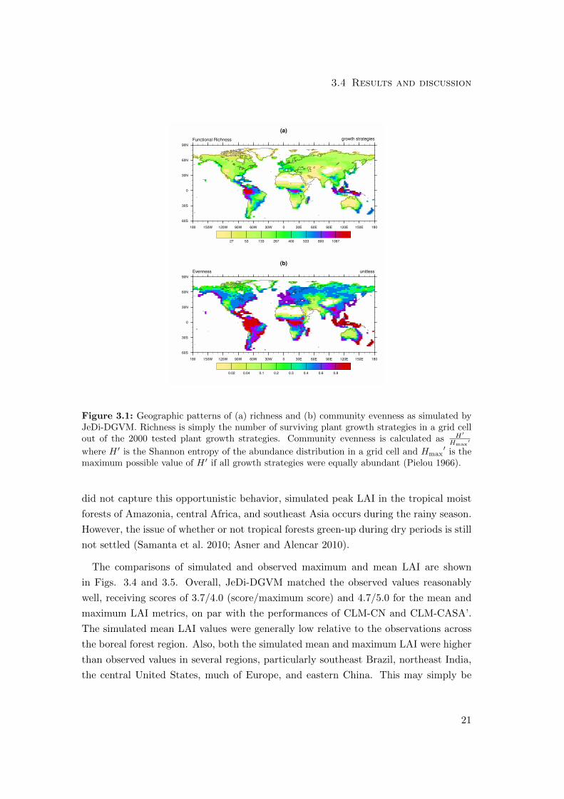
3.4.1 Biodiversity patterns
In contrast to standard DGVMs, the broad sampling across a multi-dimensional trait
space allows JeDi-DGVM to provide insight into potential plant biodiversity through
an examination of the simulated functional richness (the number of sampled plants
that survive in a grid cell). The geographic pattern of simulated functional richness
(Fig. 3.1a) is highly and significantly (r2 = 0.71) correlated with a map of vascular
plant species richness derived from observations (Kreft and Jetz 2007). Out of the 2000
randomly-assembled plant growth strategies, 1411 growth strategies survived in at least
one grid cell and the maximum value for a single grid cell was 1322 in western Amazonia.
These fractions of surviving growth strategies are much higher than those reported by
KM2000. This is likely attributable to the difference in the survival criterion. In the
earlier model of KM2000, the criteria for survival was whether or not a growth strategy
was able to produce more seed carbon over its lifetime than its initial amount of seed
carbon. Here, the criterion for survival was simply whether or not a growth strategy
was able to maintain a positive carbon balance. Nonetheless, JeDi-DGVM is still able
19
Chapter 3 JeDi-DGVM overview and evaluation
to reproduce the observed broad global pattern of plant diversity through mechanistic
environmental filtering due to functional trade-offs, and without invoking historical,
competitive, or other factors.
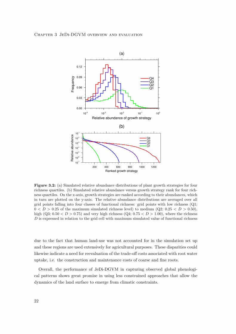
The mean relative abundance distributions for four richness classes (Fig. 3.2a) are
similar in shape to left-skewed log-normal distributions commonly observed throughout
nature (McGill et al. 2007). The left skewness means that rare species are greater
in number than abundant ones, another commonly observed attribute, especially in
tropical rainforests (Hubbell 1997). With increasing levels of functional richness, the
mean as well as the variance of the relative abundance distribution successively shifts to
lower values. We also see that there is not necessarily one optimal combination of trait
parameters for obtaining high biomass in an environment, but often many differing
growth strategies can reach similarly high levels of fitness (cf. Marks and Lechowicz
2006; Marks 2007). As the climate becomes less constraining, in terms of increasing
availability of light and precipitation, the range of feasible plant growth strategies
increases. The ranked abundances of growth strategies (Fig. 3.2b) clearly show that
the simulated relative abundances become increasingly even with higher richness. This
pattern is also evident when visually comparing the maps of simulated function richness
(Fig. 3.1a) and community evenness (Fig. 3.1b). This simulated trend towards greater
evenness in more productive regions qualitatively reproduces the observed trend in
rank-abundance plots of forests that show a much steeper decline in abundance in
boreal forests than in tropical rainforests (Hubbell 1979, 1997).
3.4.2 Phenology
For the C-LAMP phase metric, JeDi-DGVM received a score of 5.0 out of 6, performing
comparably with the two other land surface models (CLM-CN and CLM-CASA’) pre-
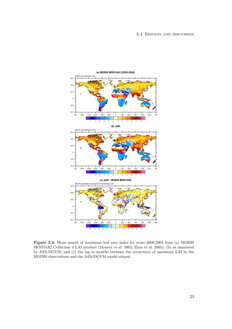
viously evaluated in Randerson et al. (2009). Fig. 3.3 shows the comparison between
the simulated and observed month of maximum LAI. The simulated timing of peak LAI
matched observations reasonably well in the moisture-limited grassland and savannah
regions of South America, Africa, and Australia. There were two clear patterns of bias,
however. First, like CLM-CN and CLM-CASA’, JeDi-DGVM simulated maximum
LAI occuring about one month later than the MODIS observations across much of the
northern hemisphere. Second, in the MODIS dataset, leaf area follows the seasonality
of incident solar radiation across large parts of the Amazon basin, peaking during the
early to mid part of the dry season when radiation levels are high and deep-rooted
vegetation still has access to sufficient moisture (Myneni et al. 2007). JeDi-DGVM
20
3.4 Results and discussion
Figure 3.1: Geographic patterns of (a) richness and (b) community evenness as simulated byJeDi-DGVM. Richness is simply the number of surviving plant growth strategies in a grid cellout of the 2000 tested plant growth strategies. Community evenness is calculated as H′
Hmax′
where H ′ is the Shannon entropy of the abundance distribution in a grid cell and Hmax′ is the
maximum possible value of H ′ if all growth strategies were equally abundant (Pielou 1966).
did not capture this opportunistic behavior, simulated peak LAI in the tropical moist
forests of Amazonia, central Africa, and southeast Asia occurs during the rainy season.
However, the issue of whether or not tropical forests green-up during dry periods is still
not settled (Samanta et al. 2010; Asner and Alencar 2010).
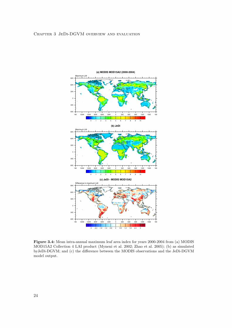
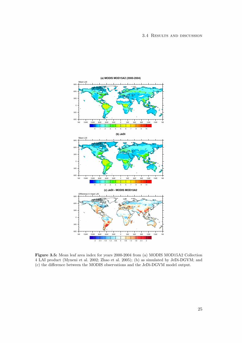
The comparisons of simulated and observed maximum and mean LAI are shown
in Figs. 3.4 and 3.5. Overall, JeDi-DGVM matched the observed values reasonably
well, receiving scores of 3.7/4.0 (score/maximum score) and 4.7/5.0 for the mean and
maximum LAI metrics, on par with the performances of CLM-CN and CLM-CASA’.
The simulated mean LAI values were generally low relative to the observations across
the boreal forest region. Also, both the simulated mean and maximum LAI were higher
than observed values in several regions, particularly southeast Brazil, northeast India,
the central United States, much of Europe, and eastern China. This may simply be
21
Chapter 3 JeDi-DGVM overview and evaluation
Figure 3.2: (a) Simulated relative abundance distributions of plant growth strategies for fourrichness quartiles. (b) Simulated relative abundance versus growth strategy rank for four rich-ness quartiles. On the x-axis, growth strategies are ranked according to their abundances, whichin turn are plotted on the y-axis. The relative abundance distributions are averaged over allgrid points falling into four classes of functional richness: grid points with low richness (Q1;0 < D > 0.25 of the maximum simulated richness level) to medium (Q2; 0.25 < D > 0.50),high (Q3; 0.50 < D > 0.75) and very high richness (Q4; 0.75 < D > 1.00), where the richnessD is expressed in relation to the grid cell with maximum simulated value of functional richness
due to the fact that human land-use was not accounted for in the simulation set up
and these regions are used extensively for agricultural purposes. These disparities could
likewise indicate a need for reevaluation of the trade-off costs associated with root water
uptake, i.e. the construction and maintenance costs of coarse and fine roots.
Overall, the performance of JeDi-DGVM in capturing observed global phenologi-
cal patterns shows great promise in using less constrained approaches that allow the
dynamics of the land surface to emerge from climatic constraints.
22
3.4 Results and discussion
Figure 3.3: Mean month of maximum leaf area index for years 2000-2004 from (a) MODISMOD15A2 Collection 4 LAI product (Myneni et al. 2002; Zhao et al. 2005); (b) as simulatedby JeDi-DGVM; and (c) the lag in months between the occurrence of maximum LAI in theMODIS observations and the JeDi-DGVM model output.
23
Chapter 3 JeDi-DGVM overview and evaluation
Figure 3.4: Mean intra-annual maximum leaf area index for years 2000-2004 from (a) MODISMOD15A2 Collection 4 LAI product (Myneni et al. 2002; Zhao et al. 2005); (b) as simulatedbyJeDi-DGVM; and (c) the difference between the MODIS observations and the JeDi-DGVMmodel output.
24
3.4 Results and discussion
Figure 3.5: Mean leaf area index for years 2000-2004 from (a) MODIS MOD15A2 Collection4 LAI product (Myneni et al. 2002; Zhao et al. 2005); (b) as simulated by JeDi-DGVM; and(c) the difference between the MODIS observations and the JeDi-DGVM model output.
25
Chapter 3 JeDi-DGVM overview and evaluation
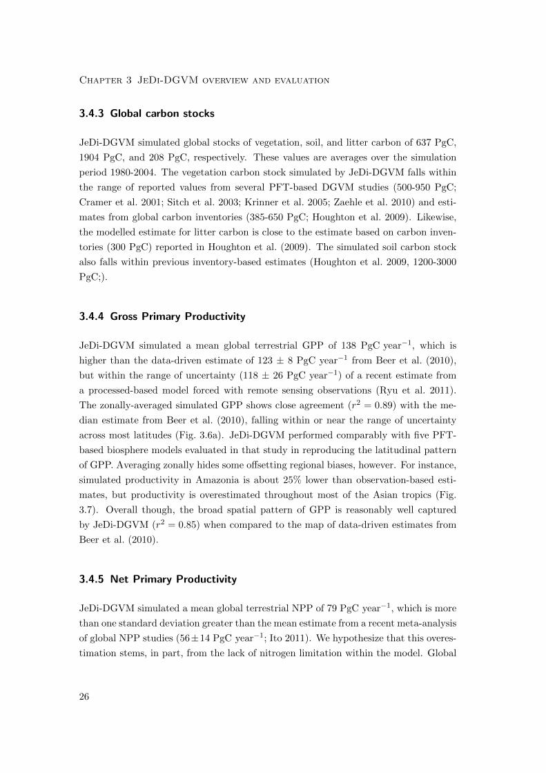
3.4.3 Global carbon stocks
JeDi-DGVM simulated global stocks of vegetation, soil, and litter carbon of 637 PgC,
1904 PgC, and 208 PgC, respectively. These values are averages over the simulation
period 1980-2004. The vegetation carbon stock simulated by JeDi-DGVM falls within
the range of reported values from several PFT-based DGVM studies (500-950 PgC;
Cramer et al. 2001; Sitch et al. 2003; Krinner et al. 2005; Zaehle et al. 2010) and esti-
mates from global carbon inventories (385-650 PgC; Houghton et al. 2009). Likewise,
the modelled estimate for litter carbon is close to the estimate based on carbon inven-
tories (300 PgC) reported in Houghton et al. (2009). The simulated soil carbon stock
also falls within previous inventory-based estimates (Houghton et al. 2009, 1200-3000
PgC;).
3.4.4 Gross Primary Productivity
JeDi-DGVM simulated a mean global terrestrial GPP of 138 PgC year−1, which is
higher than the data-driven estimate of 123 ± 8 PgC year−1 from Beer et al. (2010),
but within the range of uncertainty (118 ± 26 PgC year−1) of a recent estimate from
a processed-based model forced with remote sensing observations (Ryu et al. 2011).
The zonally-averaged simulated GPP shows close agreement (r2 = 0.89) with the me-
dian estimate from Beer et al. (2010), falling within or near the range of uncertainty
across most latitudes (Fig. 3.6a). JeDi-DGVM performed comparably with five PFT-
based biosphere models evaluated in that study in reproducing the latitudinal pattern
of GPP. Averaging zonally hides some offsetting regional biases, however. For instance,
simulated productivity in Amazonia is about 25% lower than observation-based esti-
mates, but productivity is overestimated throughout most of the Asian tropics (Fig.
3.7). Overall though, the broad spatial pattern of GPP is reasonably well captured
by JeDi-DGVM (r2 = 0.85) when compared to the map of data-driven estimates from
Beer et al. (2010).
3.4.5 Net Primary Productivity
JeDi-DGVM simulated a mean global terrestrial NPP of 79 PgC year−1, which is more
than one standard deviation greater than the mean estimate from a recent meta-analysis
of global NPP studies (56±14 PgC year−1; Ito 2011). We hypothesize that this overes-
timation stems, in part, from the lack of nitrogen limitation within the model. Global
26
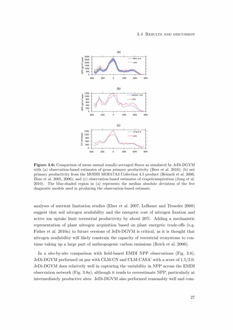
3.4 Results and discussion
Figure 3.6: Comparison of mean annual zonally-averaged fluxes as simulated by JeDi-DGVMwith (a) observation-based estimates of gross primary productivity (Beer et al. 2010); (b) netprimary productivity from the MODIS MOD17A3 Collection 4.5 product (Heinsch et al. 2006;Zhao et al. 2005, 2006); and (c) observation-based estimates of evapotranspiration (Jung et al.2010). The blue-shaded region in (a) represents the median absolute deviation of the fivediagnostic models used in producing the observation-based estimate.
analyses of nutrient limitation studies (Elser et al. 2007; LeBauer and Treseder 2008)
suggest that soil nitrogen availability and the energetic cost of nitrogen fixation and
active ion uptake limit terrestrial productivity by about 20%. Adding a mechanistic
representation of plant nitrogen acquisition based on plant energetic trade-offs (e.g.
Fisher et al. 2010a) to future versions of JeDi-DGVM is critical, as it is thought that
nitrogen availability will likely constrain the capacity of terrestrial ecosystems to con-
tinue taking up a large part of anthropogenic carbon emissions (Reich et al. 2006).
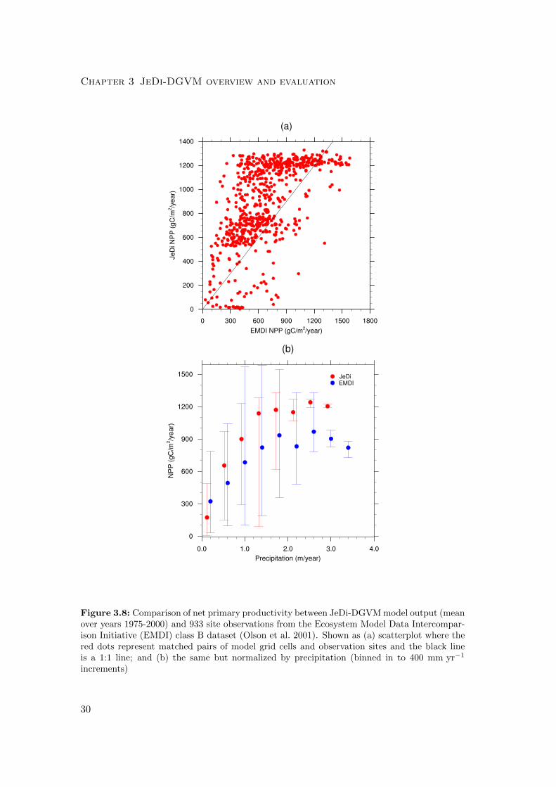
In a site-by-site comparison with field-based EMDI NPP observations (Fig. 3.8),
JeDi-DGVM performed on par with CLM-CN and CLM-CASA’ with a score of 1.5/2.0.
JeDi-DGVM does relatively well in capturing the variability in NPP across the EMDI
observation network (Fig. 3.8a), although it tends to overestimate NPP, particularly at
intermediately productive sites. JeDi-DGVM also performed reasonably well and com-
27
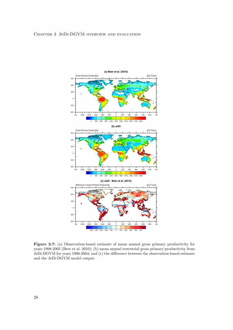
Chapter 3 JeDi-DGVM overview and evaluation
Figure 3.7: (a) Observation-based estimate of mean annual gross primary productivity foryears 1998-2005 (Beer et al. 2010); (b) mean annual terrestrial gross primary productivity fromJeDi-DGVM for years 1998-2004; and (c) the difference between the observation-based estimateand the JeDi-DGVM model output.
28
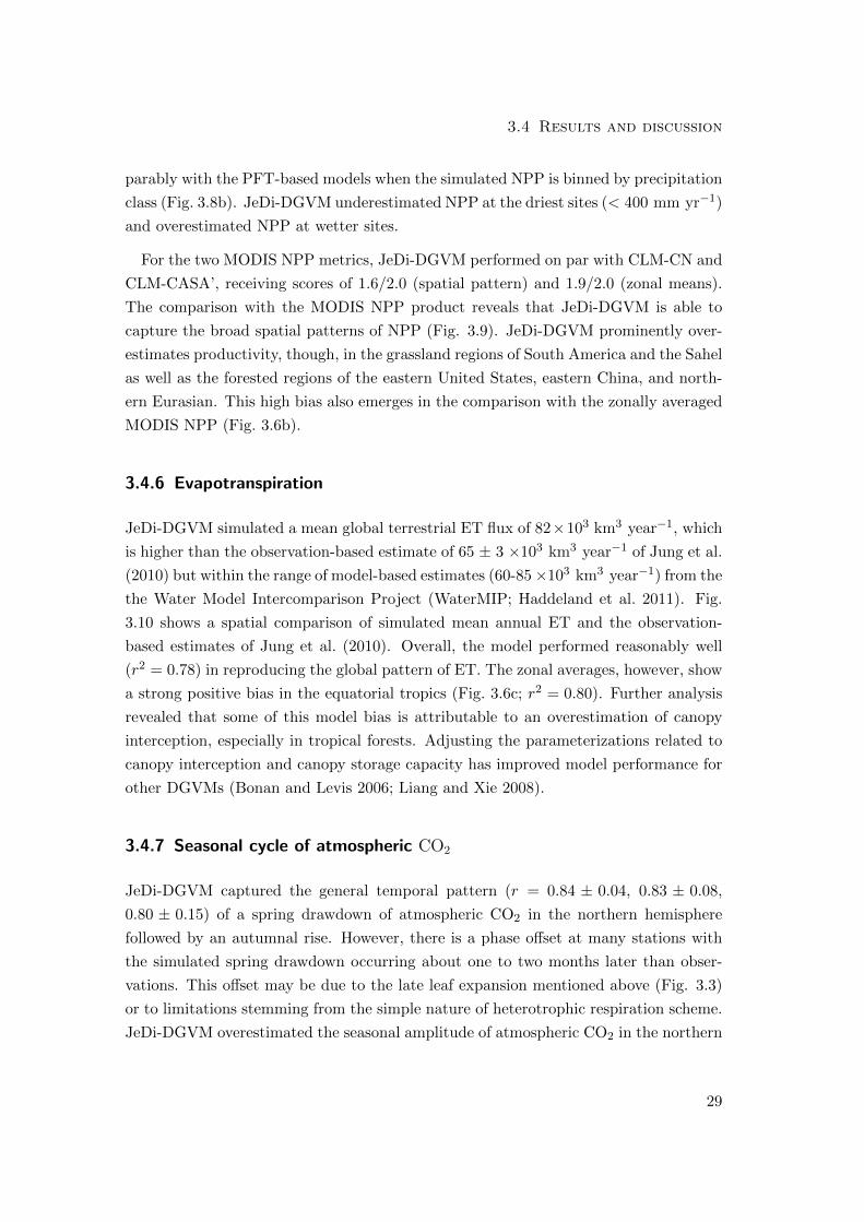
3.4 Results and discussion
parably with the PFT-based models when the simulated NPP is binned by precipitation
class (Fig. 3.8b). JeDi-DGVM underestimated NPP at the driest sites (< 400 mm yr−1)
and overestimated NPP at wetter sites.
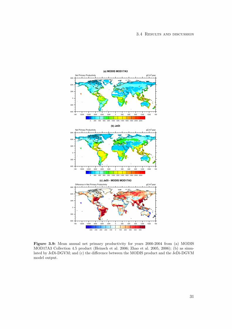
For the two MODIS NPP metrics, JeDi-DGVM performed on par with CLM-CN and
CLM-CASA’, receiving scores of 1.6/2.0 (spatial pattern) and 1.9/2.0 (zonal means).
The comparison with the MODIS NPP product reveals that JeDi-DGVM is able to
capture the broad spatial patterns of NPP (Fig. 3.9). JeDi-DGVM prominently over-
estimates productivity, though, in the grassland regions of South America and the Sahel
as well as the forested regions of the eastern United States, eastern China, and north-
ern Eurasian. This high bias also emerges in the comparison with the zonally averaged
MODIS NPP (Fig. 3.6b).
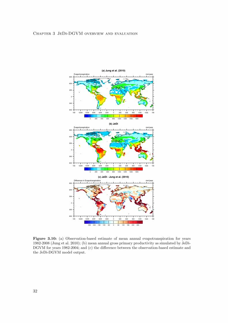
3.4.6 Evapotranspiration
JeDi-DGVM simulated a mean global terrestrial ET flux of 82×103 km3 year−1, which
is higher than the observation-based estimate of 65 ± 3 ×10³ km3 year−1 of Jung et al.
(2010) but within the range of model-based estimates (60-85×103 km3 year−1) from the
the Water Model Intercomparison Project (WaterMIP; Haddeland et al. 2011). Fig.
3.10 shows a spatial comparison of simulated mean annual ET and the observation-
based estimates of Jung et al. (2010). Overall, the model performed reasonably well
(r2 = 0.78) in reproducing the global pattern of ET. The zonal averages, however, show
a strong positive bias in the equatorial tropics (Fig. 3.6c; r2 = 0.80). Further analysis
revealed that some of this model bias is attributable to an overestimation of canopy
interception, especially in tropical forests. Adjusting the parameterizations related to
canopy interception and canopy storage capacity has improved model performance for
other DGVMs (Bonan and Levis 2006; Liang and Xie 2008).
3.4.7 Seasonal cycle of atmospheric CO2
JeDi-DGVM captured the general temporal pattern (r = 0.84 ± 0.04, 0.83 ± 0.08,
0.80 ± 0.15) of a spring drawdown of atmospheric CO2 in the northern hemisphere
followed by an autumnal rise. However, there is a phase offset at many stations with
the simulated spring drawdown occurring about one to two months later than obser-
vations. This offset may be due to the late leaf expansion mentioned above (Fig. 3.3)
or to limitations stemming from the simple nature of heterotrophic respiration scheme.
JeDi-DGVM overestimated the seasonal amplitude of atmospheric CO2 in the northern
29
Chapter 3 JeDi-DGVM overview and evaluation
Figure 3.8: Comparison of net primary productivity between JeDi-DGVM model output (meanover years 1975-2000) and 933 site observations from the Ecosystem Model Data Intercompar-ison Initiative (EMDI) class B dataset (Olson et al. 2001). Shown as (a) scatterplot where thered dots represent matched pairs of model grid cells and observation sites and the black lineis a 1:1 line; and (b) the same but normalized by precipitation (binned in to 400 mm yr−1
increments)
30
3.4 Results and discussion
Figure 3.9: Mean annual net primary productivity for years 2000-2004 from (a) MODISMOD17A3 Collection 4.5 product (Heinsch et al. 2006; Zhao et al. 2005, 2006); (b) as simu-lated by JeDi-DGVM; and (c) the difference between the MODIS product and the JeDi-DGVMmodel output.
31
Chapter 3 JeDi-DGVM overview and evaluation
Figure 3.10: (a) Observation-based estimate of mean annual evapotranspiration for years1982-2008 (Jung et al. 2010); (b) mean annual gross primary productivity as simulated by JeDi-DGVM for years 1982-2004; and (c) the difference between the observation-based estimate andthe JeDi-DGVM model output.
32

3.4 Results and discussion
hemisphere, particularly in the middle and high latitude bands. The ratios of simu-
lated to observed amplitudes were 1.23±0.08, 1.33±0.26, and 1.10±0.16, for the high,
middle, and equatorial latitude bands, respectively. This overestimation in seasonal
amplitude is directly attributable to the overestimation of NPP in those regions. Fig.
3.11 illustrates the reasonably good agreement between the simulated seasonal CO2 cy-
cle and GLOBALVIEW measurements at a high latitude (Point Barrow, Alaska, United
States), a mid-latitude (Niwot Ridge, Colorado, United States), and an equatorial sta-
tion (Mauna Loa, Hawaii, United States). The results for all GLOBALVIEW stations
considered here are summarized in a Taylor diagram (Taylor 2001) in Fig. 3.12.
Overall, JeDi-DGVM performed better than CLM-CN and CLM-CASA’ on this met-
ric with a combined score of 11.8/15.0. It scored better than both PFT-based models
on the measure of amplitude agreement and fell between the scores of those models on
the measure of phase agreement.
3.4.8 Net terrestrial carbon exchange
The net terrestrial carbon sink simulated by JeDi-DGVM is compatible with decadal
budgets of the global carbon cycle given the uncertainties regarding the oceanic and
anthropogenic fluxes. For the 1980s, JeDi-DGVM simulated a global terrestrial car-
bon flux of −2.89 PgC yr−1 (negative values indicate a net uptake of carbon by the
terrestrial biosphere), which lies within the range of uncertainty from the IPCC (-3.8
to 0.3 PgC yr−1; Denman et al. 2007). In agreement with the IPCC carbon budgets,
JeDi-DGVM simulated a larger carbon sink in the 1990s (−3.35 PgC yr−1), which also
lies within the IPCC range of -4.3 to -1.0 PgC yr−1 (Denman et al. 2007). The model
estimates presented here suggest a stronger land carbon sink than previous DGVM
studies (1.2-2.75 PgC; Sitch et al. 2008; Randerson et al. 2009).
JeDi-DGVM captured the magnitude of interannual variability of terrestrial NEE
quite well (σ = 0.94 Pg yr−1) when compared to the TRANSCOM-derived estimates
(σ = 1.04 PgC yr−1)or the period 1988-2004. The model results are also moderately
correlated (r = 0.42; p < 0.05) with the year-to-year TRANSCOM anomalies. The
simulated anomalies fell within one standard deviation of the multi-model TRANSCOM
mean in 12 of the 17 years.
The model captured the strong positive anomaly associated with the 1998 El Nino
event, but not the similarly strong anomaly in 1997. The rapid growth rate of at-
mospheric CO2 in 1997 has been linked with large peat and forest fires in the Asian
33

Chapter 3 JeDi-DGVM overview and evaluation
Month
Detre
nded
CO
2 m
ixin
g ra
tio (p
pm) a) Barrow
b) Niwot Ridge
c) Mauna Loa
GLOBALVIEW JeDi-DGVM + TRANSCOM
Figure 3.11: Mean seasonal cycle of atmospheric CO2 at (a) Barrow, Alaska (71 ◦N), (b) NiwotRidge, Colorado (40 ◦N), (c) Mauna Loa, Hawaii (20 ◦N) for years 1991-2000. The dashed bluelines represent the observations from the GLOBALVIEW dataset (Masarie and Tans 1995).The JeDi-DGVM estimates were obtained by combining the simulated NEE fluxes with themonthly impulse response functions (Gurney et al. 2004) of the 13 TRANSCOM atmospherictracer transport models. The red line represents the mean of the model estimates. The lightred shaded region represents one standard deviation around the multimodel mean.
tropics (Page et al. 2002; van der Werf et al. 2008). Incorporating mechanistic rep-
resentations of fire (e.g. Thonicke et al. 2008) and peat dynamics (e.g. Kleinen et al.
2012) in JeDi-DGVM may improve performance on this metric.
JeDi-DGVM was also not able to capture the negative anomaly in 1992-1993. This
drawdown has been associated with climate impacts from the Mount Pinatubo eruption,
including an increase in diffuse radiation due to elevated stratospheric aerosol loads
(Gu et al. 2003; Mercado et al. 2009). A more detailed canopy radiation transfer model
(e.g. Drewry et al. 2010) would be required to to appropriately capture the effects
of diffuse light on vegetation productivity. If the two years strongly affected by the
Pinatubo eruption (1992-1993) are excluded, the model time series is highly correlated
(r = 0.63; p < 0.01) with the interannual TRANSCOM anomalies.
34
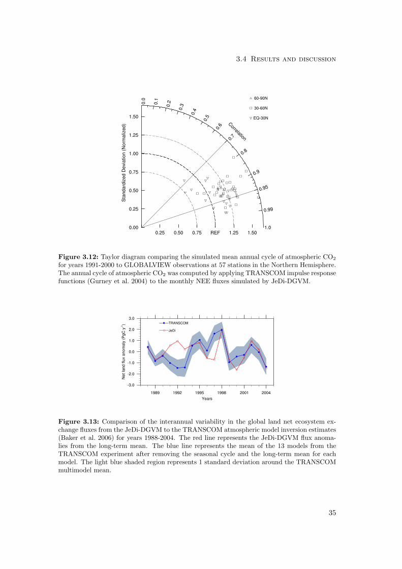
3.4 Results and discussion
Figure 3.12: Taylor diagram comparing the simulated mean annual cycle of atmospheric CO2
for years 1991-2000 to GLOBALVIEW observations at 57 stations in the Northern Hemisphere.The annual cycle of atmospheric CO2 was computed by applying TRANSCOM impulse responsefunctions (Gurney et al. 2004) to the monthly NEE fluxes simulated by JeDi-DGVM.
Figure 3.13: Comparison of the interannual variability in the global land net ecosystem ex-change fluxes from the JeDi-DGVM to the TRANSCOM atmospheric model inversion estimates(Baker et al. 2006) for years 1988-2004. The red line represents the JeDi-DGVM flux anoma-lies from the long-term mean. The blue line represents the mean of the 13 models from theTRANSCOM experiment after removing the seasonal cycle and the long-term mean for eachmodel. The light blue shaded region represents 1 standard deviation around the TRANSCOMmultimodel mean.
35
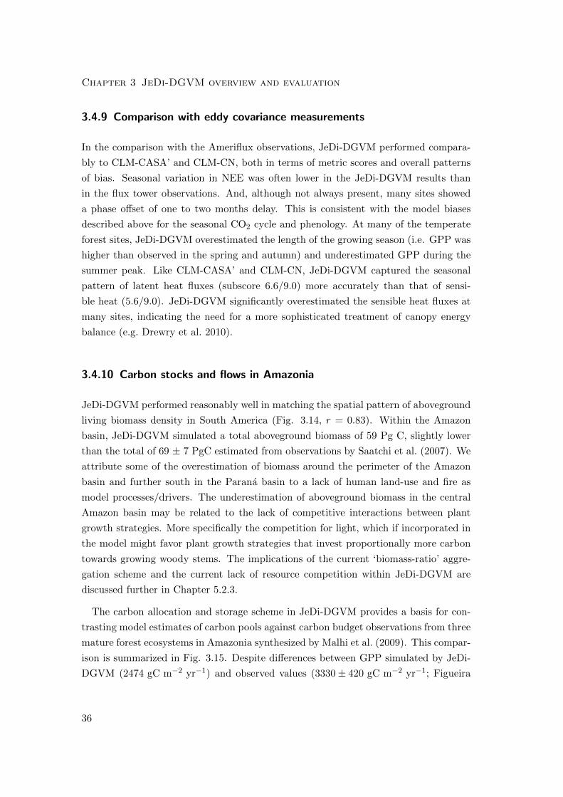
Chapter 3 JeDi-DGVM overview and evaluation
3.4.9 Comparison with eddy covariance measurements
In the comparison with the Ameriflux observations, JeDi-DGVM performed compara-
bly to CLM-CASA’ and CLM-CN, both in terms of metric scores and overall patterns
of bias. Seasonal variation in NEE was often lower in the JeDi-DGVM results than
in the flux tower observations. And, although not always present, many sites showed
a phase offset of one to two months delay. This is consistent with the model biases
described above for the seasonal CO2 cycle and phenology. At many of the temperate
forest sites, JeDi-DGVM overestimated the length of the growing season (i.e. GPP was
higher than observed in the spring and autumn) and underestimated GPP during the
summer peak. Like CLM-CASA’ and CLM-CN, JeDi-DGVM captured the seasonal
pattern of latent heat fluxes (subscore 6.6/9.0) more accurately than that of sensi-
ble heat (5.6/9.0). JeDi-DGVM significantly overestimated the sensible heat fluxes at
many sites, indicating the need for a more sophisticated treatment of canopy energy
balance (e.g. Drewry et al. 2010).
3.4.10 Carbon stocks and flows in Amazonia
JeDi-DGVM performed reasonably well in matching the spatial pattern of aboveground
living biomass density in South America (Fig. 3.14, r = 0.83). Within the Amazon
basin, JeDi-DGVM simulated a total aboveground biomass of 59 Pg C, slightly lower
than the total of 69 ± 7 PgC estimated from observations by Saatchi et al. (2007). We
attribute some of the overestimation of biomass around the perimeter of the Amazon
basin and further south in the Parana basin to a lack of human land-use and fire as
model processes/drivers. The underestimation of aboveground biomass in the central
Amazon basin may be related to the lack of competitive interactions between plant
growth strategies. More specifically the competition for light, which if incorporated in
the model might favor plant growth strategies that invest proportionally more carbon
towards growing woody stems. The implications of the current ‘biomass-ratio’ aggre-
gation scheme and the current lack of resource competition within JeDi-DGVM are
discussed further in Chapter 5.2.3.
The carbon allocation and storage scheme in JeDi-DGVM provides a basis for con-
trasting model estimates of carbon pools against carbon budget observations from three
mature forest ecosystems in Amazonia synthesized by Malhi et al. (2009). This compar-
ison is summarized in Fig. 3.15. Despite differences between GPP simulated by JeDi-
DGVM (2474 gC m−2 yr−1) and observed values (3330± 420 gC m−2 yr−1; Figueira
36
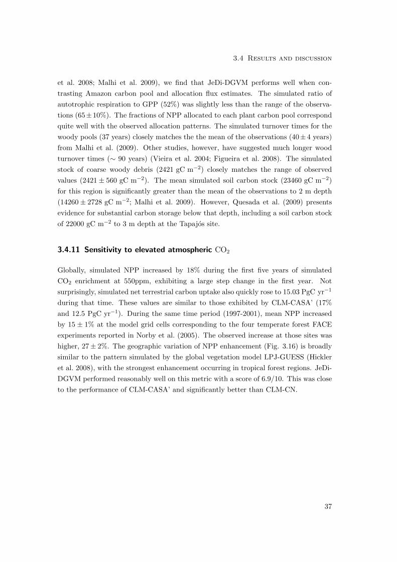
3.4 Results and discussion
et al. 2008; Malhi et al. 2009), we find that JeDi-DGVM performs well when con-
trasting Amazon carbon pool and allocation flux estimates. The simulated ratio of
autotrophic respiration to GPP (52%) was slightly less than the range of the observa-
tions (65±10%). The fractions of NPP allocated to each plant carbon pool correspond
quite well with the observed allocation patterns. The simulated turnover times for the
woody pools (37 years) closely matches the the mean of the observations (40± 4 years)
from Malhi et al. (2009). Other studies, however, have suggested much longer wood
turnover times (∼ 90 years) (Vieira et al. 2004; Figueira et al. 2008). The simulated
stock of coarse woody debris (2421 gC m−2) closely matches the range of observed
values (2421± 560 gC m−2). The mean simulated soil carbon stock (23460 gC m−2)
for this region is significantly greater than the mean of the observations to 2 m depth
(14260± 2728 gC m−2; Malhi et al. 2009). However, Quesada et al. (2009) presents
evidence for substantial carbon storage below that depth, including a soil carbon stock
of 22000 gC m−2 to 3 m depth at the Tapajos site.
3.4.11 Sensitivity to elevated atmospheric CO2
Globally, simulated NPP increased by 18% during the first five years of simulated
CO2 enrichment at 550ppm, exhibiting a large step change in the first year. Not
surprisingly, simulated net terrestrial carbon uptake also quickly rose to 15.03 PgC yr−1
during that time. These values are similar to those exhibited by CLM-CASA’ (17%
and 12.5 PgC yr−1). During the same time period (1997-2001), mean NPP increased
by 15 ± 1% at the model grid cells corresponding to the four temperate forest FACE
experiments reported in Norby et al. (2005). The observed increase at those sites was
higher, 27± 2%. The geographic variation of NPP enhancement (Fig. 3.16) is broadly
similar to the pattern simulated by the global vegetation model LPJ-GUESS (Hickler
et al. 2008), with the strongest enhancement occurring in tropical forest regions. JeDi-
DGVM performed reasonably well on this metric with a score of 6.9/10. This was close
to the performance of CLM-CASA’ and significantly better than CLM-CN.
37
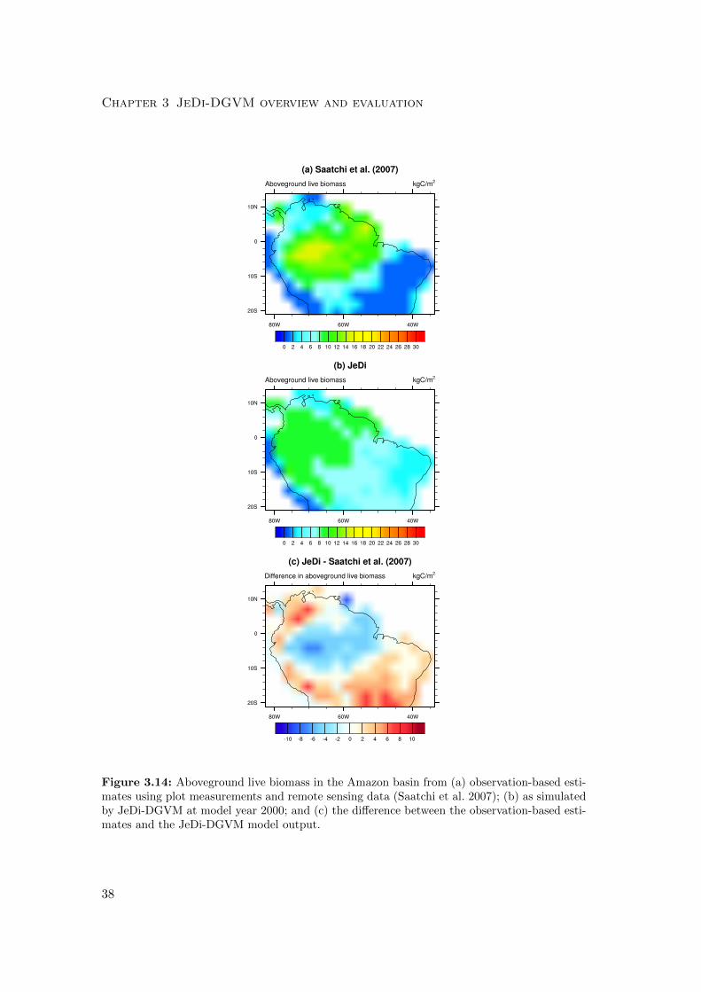
Chapter 3 JeDi-DGVM overview and evaluation
Figure 3.14: Aboveground live biomass in the Amazon basin from (a) observation-based esti-mates using plot measurements and remote sensing data (Saatchi et al. 2007); (b) as simulatedby JeDi-DGVM at model year 2000; and (c) the difference between the observation-based esti-mates and the JeDi-DGVM model output.
38
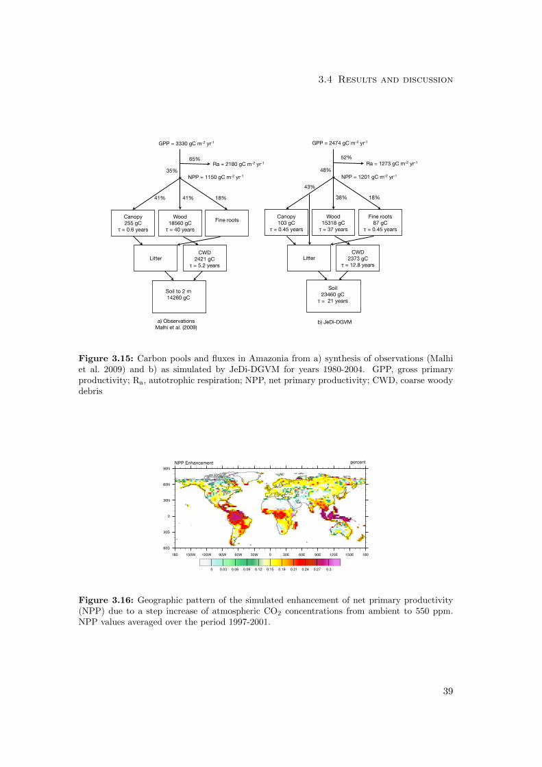
3.4 Results and discussion
Canopy103 gC
τ = 0.45 years
Wood15318 gC
τ = 37 years
Fine roots87 gC
τ = 0.45 years
Litter
Soil23460 gC
τ = 21 years
GPP = 2474 gC m-2 yr-1
Ra = 1273 gC m-2 yr-1
NPP = 1201 gC m-2 yr-1
18%38%
43%
52%
48%
CWD2373 gC
τ = 12.8 years
Canopy255 gC
τ = 0.6 years
Wood18560 gC
τ = 40 yearsFine roots
LitterCWD
2421 gCτ = 5.2 years
GPP = 3330 gC m-2 yr-1
Ra = 2180 gC m-2 yr-1
NPP = 1150 gC m-2 yr-1
18%41%41%
a) ObservationsMalhi et al. (2009)
65%
35%
b) JeDi-DGVM
Soil to 2 m14260 gC
Figure 3.15: Carbon pools and fluxes in Amazonia from a) synthesis of observations (Malhiet al. 2009) and b) as simulated by JeDi-DGVM for years 1980-2004. GPP, gross primaryproductivity; Ra, autotrophic respiration; NPP, net primary productivity; CWD, coarse woodydebris
Figure 3.16: Geographic pattern of the simulated enhancement of net primary productivity(NPP) due to a step increase of atmospheric CO2 concentrations from ambient to 550 ppm.NPP values averaged over the period 1997-2001.
39
Chapter 3 JeDi-DGVM overview and evaluation
3.5 Summary of model evaluation
Overall, JeDi-DGVM received a score of 68.2 (out of 100 possible), exceeding the scores
of the two PFT-based models (CLM-CASA’; 65.7 and CLM-CN; 58.4) evaluated in Ran-
derson et al. (2009). The scores of the individual metrics are summarized in Table 3.1.
JeDi-DGVM matched or exceeded the performance of at least one of the other models
on almost every metric. The two exceptions were the comparisons with estimates of
interannual terrestrial carbon exchange and fire emissions. The results of this eval-
uation imply that that the bottom-up functional trade-off approach of JeDi-DGVM,
linked with an aggregation mechanism based on the ‘biomass-ratio’ hypothesis, is capa-
ble of simulating the broad-scale patterns of terrestrial biogeochemistry at least as well
as two other state-of-the-art terrestrial biosphere models based on the dominant PFT
paradigm. We have also shown that unlike PFT-based DGVMs, JeDi-DGVM is able
to mechanistically represent the large-scale biogeographical patterns of plant species
richness, community evenness, and relative abundance distributions, opening avenues
to explore the impacts of future climate variability on terrestrial ecosystem composition
and function in a much less constrained way than has been previously performed.
40
Chapter 4
Quantifying functional diversity-biospheric
functioning relationships
4.1 Introduction
Ecologists have long suspected that plant functional diversity influences the magnitude
and variability of ecosystem functioning. This thinking is well illustrated by a passage
from Charles Darwin’s unfinished manuscript Natural Selection, which was later edited
and published nearly 100 years after his death (Darwin 1987):
We may . . . assert that a greater absolute amount of life can be supported;
. . . when life is developed under many & widely different forms, than when
under a few & allied forms; – the fairest measure of the amount of life,
being probably the amount chemical composition within a given period.
Imagine the case of an island, peopled with only three or four plants of
the same order all well adapted to their conditions of life, & by three or
four insects of the same order; the surface would no doubt be pretty well
clothed with plants & there would many individuals of these species; . . . but
assuredly there would seasons of the year, peculiar & intermediate stations,
. . . which would not be well searched for food, & the amount of life would
be consequently less, than if our island had been stocked with hundreds of
forms, belonging to the most diversified orders.
Field and laboratory experiments in the last several decades have confirmed Darwin’s
thinking. Diversity manipulation experiments have shown that higher levels of func-
tional diversity lead to higher ecosystem productivity (Cardinale et al. 2011; Hooper
et al. 2005; Hector et al. 1999; Flombaum and Sala 2008) and lower temporal variability
of ecosystem functioning (Tilman et al. 2006; Proulx et al. 2010; Ives and Carpenter
41
Chapter 4 Diversity and biospheric functioning
2007; Balvanera et al. 2006). There is a growing consensus in the ecological science
community that human-induced biodiversity loss is a threat to the ecosystem services
we rely upon and thus our well-being (Dıaz et al. 2006). At the same time, the loss of
species and, more importantly, the functional traits of those species is likely going to
reduce the ability of ecosystems to adapt to environmental changes including ongoing
global warming (Elmqvist et al. 2003). This ability of ecosystems to adapt to changes
and to maintain their functioning in the face of those change is referred to as resilience
(Peterson et al. 1998).
In many ways, current global vegetation models (Dynamic Global Vegetation Models,
DGVMs) based on the PFT paradigm are simulating Darwin’s island. DGVMs reduce
the immense functional diversity of terrestrial vegetation to handful of PFTs. Recent
studies using trait data collected and compiled from all over the globe have shown that
for several functional traits, there is greater variation within PFTs than between PFTs
(Wright et al. 2005; Reich et al. 2007; Kattge et al. 2011). Current models, however,
can only use a single parameter value to represent this large within–PFT variation.
Model-data assimilation studies (Groenendijk et al. 2011; Alton 2011) have shown that
the coarse representation of functional diversity provided by these PFT schemes is
insufficient for representing the full variability of vegetation parameters necessary to
accurately represent carbon cycle processes.
Based on the growing consensus regarding biodiversity-ecosystem functioning rela-
tionships, we can hypothesize that PFT-based models would underestimate productiv-
ity and overestimate the response of terrestrial ecosystems to climatic variability and
change. In this chapter, we contrast the magnitude and variability of net primary pro-
ductivity and evapotranspiration fluxes of diverse communities to those of a single, but
representative PFT. This is accomplished by running a diverse JeDi-DGVM simulation
with many plant growth strategies and where the community fluxes are aggregated
from the different strategies (the Community Weighted Functioning, ”CWF” approach
in the following) and another simulation wherein the functional diversity is reduced.
This reduction is accomplished by recreating something like a PFT by simulating only a
single plant growth strategy at each grid cell characterized by the community-weighted
functional trait parameters from the diverse simulation (the Community Weighted Trait
”CWF” approach in the following). The major difference between the two approaches
is that in the CWT approach, the community-weighted mean trait values are fixed at
the start of the simulation. In the CWF approach of the diverse communities, the
relative abundances of the growth strategies change throughout the simulation as the
climate becomes relatively more or relatively less favorable for its particular set of trait
42
4.1 Introduction
values.
The two model simulations are investigated to evaluate the role of diversity in ecosys-
tem functioning. We focus on three different aspects with regard to the functioning. We
hypothesize that the diverse representation of the terrestrial biosphere leads to a higher
productivity in the climatic mean, to greater time stability, and to greater resilience
to large climatic perturbations. In the CWF approach, altered climatic conditions
would favor different trait combinations that are better suited to these conditions. If,
for instance, conditions become wetter, then this would favor trait combinations that
can exploit the greater availability of moisture, for instance by enhancing allocation
to leaves rather than roots. This is schematically shown by the blue line in Fig. 4.1.
Likewise, when conditions become drier, productivity is likely be reduced. The extent
of this reduction can, however, be partly compensated by trait combinations that can
achieve a higher productivity at lower water availability (shown by the red curve in
Fig. 4.1). In other words, the diverse ecosystem would be better able to exploit current
climatic conditions as well as altered conditions due to climatic variability or change.
In contrast, the CWT approach only captures the average trait composition of the
mean climate, implying that the vegetation that this approach represents would likely
to be best suited and most productive under climatic mean conditions. Any deviation
from the mean climate, for instance drier or wetter conditions due to climate variability
or change, the resulting trait combination would likely not to be most suitable to the
altered conditions. This is schematically illustrated in Fig. 4.1 on the right.
To demonstrate a the potential importance of vegetation diversity to climate, we also
evaluate these simulations with respect to the differences in evapotranspiration.
43
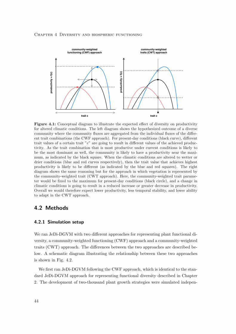
Chapter 4 Diversity and biospheric functioning
prod
uctiv
ity =
f(c)
community-weightedtraits (CWT) approach
community-weightedfunctioning (CWF) approach
trait c trait c
prod
uctiv
ity =
f(c)
Figure 4.1: Conceptual diagram to illustrate the expected effect of diversity on productivityfor altered climatic conditions. The left diagram shows the hypothesized outcome of a diversecommunity where the community fluxes are aggregated from the individual fluxes of the differ-ent trait combinations (the CWF approach). For present-day conditions (black curve), differenttrait values of a certain trait ”c” are going to result in different values of the achieved produc-tivity. As the trait combination that is most productive under current conditions is likely tobe the most dominant as well, the community is likely to have a productivity near the maxi-mum, as indicated by the black square. When the climatic conditions are altered to wetter ordrier conditions (blue and red curves respectively), then the trait value that achieves highestproductivity is likely to be different (as indicated by the blue and red squares). The rightdiagram shows the same reasoning but for the approach in which vegetation is represented bythe community-weighted trait (CWT approach). Here, the community-weighted trait parame-ter would be fixed to the maximum for present-day conditions (black circle), and a change inclimatic conditions is going to result in a reduced increase or greater decrease in productivity.Overall we would therefore expect lower productivity, less temporal stability, and lower abilityto adapt in the CWT approach.
4.2 Methods
4.2.1 Simulation setup
We ran JeDi-DGVM with two different approaches for representing plant functional di-
versity, a community-weighted functioning (CWF) approach and a community-weighted
traits (CWT) approach. The differences between the two approaches are described be-
low. A schematic diagram illustrating the relationship between these two approaches
is shown in Fig. 4.2.
We first ran JeDi-DGVM following the CWF approach, which is identical to the stan-
dard JeDi-DGVM approach for representing functional diversity described in Chapter
2. The development of two-thousand plant growth strategies were simulated indepen-
44
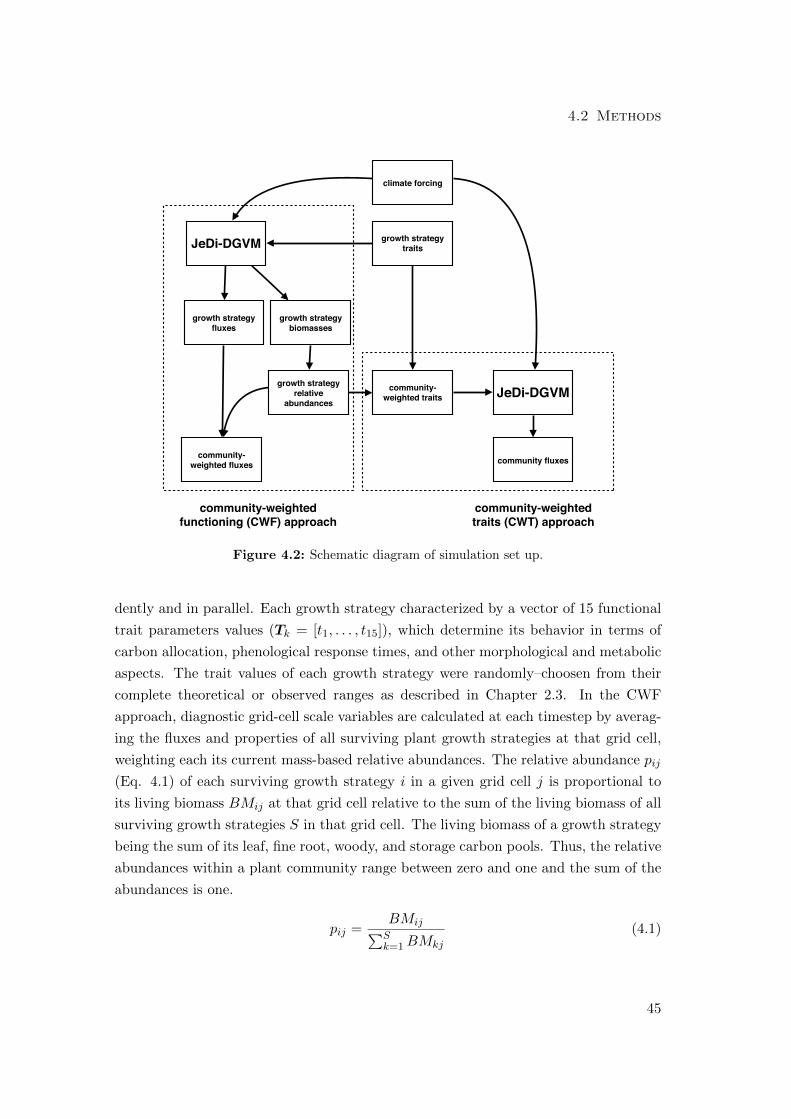
4.2 Methods
JeDi-DGVM
JeDi-DGVM
growth strategy fluxes
growth strategy biomasses
growth strategy relative
abundances
community-weighted fluxes
growth strategy traits
climate forcing
community-weighted traits
community fluxes
community-weightedtraits (CWT) approach
community-weightedfunctioning (CWF) approach
Figure 4.2: Schematic diagram of simulation set up.
dently and in parallel. Each growth strategy characterized by a vector of 15 functional
trait parameters values (Tk = [t1, . . . , t15]), which determine its behavior in terms of
carbon allocation, phenological response times, and other morphological and metabolic
aspects. The trait values of each growth strategy were randomly–choosen from their
complete theoretical or observed ranges as described in Chapter 2.3. In the CWF
approach, diagnostic grid-cell scale variables are calculated at each timestep by averag-
ing the fluxes and properties of all surviving plant growth strategies at that grid cell,
weighting each its current mass-based relative abundances. The relative abundance pij
(Eq. 4.1) of each surviving growth strategy i in a given grid cell j is proportional to
its living biomass BMij at that grid cell relative to the sum of the living biomass of all
surviving growth strategies S in that grid cell. The living biomass of a growth strategy
being the sum of its leaf, fine root, woody, and storage carbon pools. Thus, the relative
abundances within a plant community range between zero and one and the sum of the
abundances is one.
pij =BMij∑S
k=1BMkj
(4.1)
45
Chapter 4 Diversity and biospheric functioning
Following Garnier et al. (2004), we refer to these diagnostic grid-cell scale variables
as community-weighted fluxes (or properties). As an example, the NPPij of each
growth strategy i at a grid cell j is a function of its traits parameter values Ti and
the environment forcing variables Xj . The community-weighted NPP1 〈NPPj〉 for
that grid cell is the sum of the NPP fluxes of all growth strategies S at that grid cell,
weighting the contribution of each growth strategy by its mass-based relative abundance
pi,j :
〈NPPj〉 =S∑
i=1
pi,j NPPij =S∑
i=1
pi,j f (Ti,Xj) . (4.2)
In the CWT approach, we use the time-averaged relative abundances pij from the
CWF simulation to calculate the community-weighted mean trait parameters (〈Tj〉 =∑Si=1 pij Ti) at each grid cell j. We then run JeDi-DGVM with just one plant growth
strategy at each grid cell characterized by the community-weighted mean trait vector
〈Tj〉. Continuing the example from above, the community NPP NPPj in the CWT
approach is a function of the community-weighted mean trait vector 〈Tj〉 from the the
CWF approach and the same environment forcing variables Xj :
NPPj = f (〈Tj〉,Xj) = f(∑
pij Ti,Xj). (4.3)
For both approaches, JeDi-DGVM was run on a global grid at a spatial resolution of
approximately 2.8◦ by 2.8◦ resolution, covering all land areas except Antarctica. The
model was forced at a daily time step with downward shortwave and longwave radia-
tion, precipitation, and near-surface air temperature from an improved NCEP/NCAR
atmospheric reanalysis dataset (Qian et al. 2006). The atmospheric CO2 concentration
was fixed at 380 ppm throughout all simulations. We looped through the reanalysis
dataset for 1000 years, allowing the vegetation carbon pools to reach a quasi-steady
state. We used only the last 100 years of model output to evaluate the differences
between the two approaches.
We also ran two additional 100 year pertubation simulations for both approaches to
investigate the role of modelled functional diversity on ecosystem resilience to sudden
climatic change. These pertubation simulations were branched from the end of the
spin-up simulations described above. In the first pertubation, we reduced the precipi-
tation at each time step by 50%. In the second pertubation, we added 2◦ C to the air
1We adopt chevron notation (e.g. 〈NPPj〉 to denote community-aggregated fluxes and properties.
46
4.2 Methods
temperature.
4.2.2 Diversity measures
We calculated three functional diversity measures for each grid cell of the CWF simu-
lation. We use these diversity measures in the following section to help understand the
differences between the CWT and CWF simulations.
The functional richness (FR) at each grid cell is derived from the number of surviving
growth strategies (Fig. 4.3a). The FR is normalized by the maximum number of
surviving PGSs in any of the grid cells. Here, survival is defined as maintaining a
positive balance of stored assimilates. Thus, FR varies between zero for grid cells with
no surviving PGSs and one at the grid cell (or grid cells) with the maximum number
of growth strategies.
Functional evenness (FE) at each grid cell is calculated following the Pielou index
(Pielou 1966), which is the the Shannon entropy of the relative abundances pi of the
S surviving growth strategies within that grid cell, normalized by the maximized pos-
sible Shannon entropy for that community (i.e. when all growth strategies are equally
abundant). A map of simulated FE is shown in Fig. 4.3b.
FE =
∑Si=1 pi ln pi
lnS(4.4)
FE approaches zero as more and more plant biomass is found in only one or a few
growth strategies. FE is set to zero when there is one or no surviving growth strategies.
The Shannon entropy of a given community is basically a measure of uncertainty in
predicting the relative abundances of the growth strategies that compose the relative
abundance vector p = (p1, p2, . . . , pS).
Functional dispersion (FD) is calculated as the weighted mean Euclidean distance
of all growth strategies to the community-weighted centroid of all growth strategies in
47
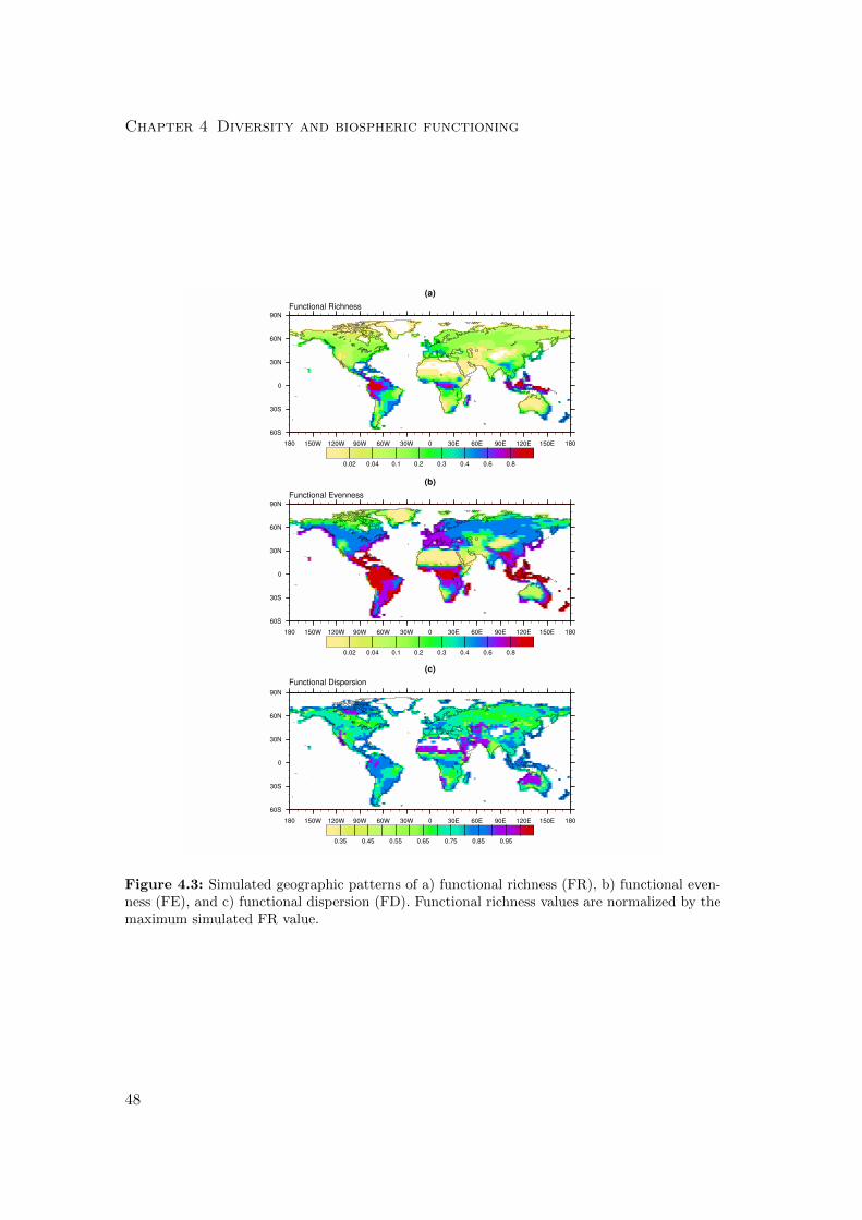
Chapter 4 Diversity and biospheric functioning
Figure 4.3: Simulated geographic patterns of a) functional richness (FR), b) functional even-ness (FE), and c) functional dispersion (FD). Functional richness values are normalized by themaximum simulated FR value.
48
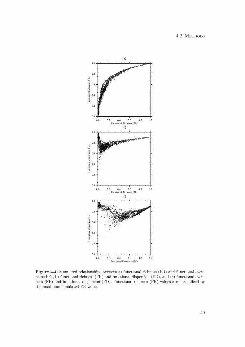
4.2 Methods
Figure 4.4: Simulated relationships between a) functional richness (FR) and functional even-ness (FE), b) functional richness (FR) and functional dispersion (FD), and (c) functional even-ness (FE) and functional dispersion (FD). Functional richness (FR) values are normalized bythe maximum simulated FR value.
49
Chapter 4 Diversity and biospheric functioning
multidimensional trait space (4.3c):
zi = ‖Ti − 〈T 〉‖ =
√√√√ n∑k=1
(tik − 〈tk〉)2 (4.5)
FD =S∑
i=1
pizi (4.6)
(4.7)
where pi is the relative abundance of growth strategy i, and zi is the distance of growth
strategy i to the community-weighted centroid 〈T 〉 (Laliberte and Legendre 2010). FD
is low when the most abundant growth strategies (possibly the only surviving growth
strategies) are all near the centroid. FD is highest when the community biomass is
dominated by a few growth strategies that differ widely in their trait values.
4.3 Results
4.3.1 Differences in mean productivity and evapotranspiration
Fig. 4.5 shows the absolute difference (top) and relative difference (bottom) between
the CWT and CWF simulations in mean NPP. The CWT simulation yielded lower NPP
than the CWF simulation in nearly all regions, however, the magnitude of this decrease
varies spatially. The relative difference in NPP varies nearly quite strongly with FR
and FE (Figs. 4.6a and 4.6b), grid cells with more surviving growth strategies and
strategies with more evenly distributed community biomass tend to have less difference
in productivity between the CWT and the CWF approaches. The relative decrease
in NPP is strongest in arid and arctic regions with high FD (Fig. 4.6c), i.e. regions
where the distribution of community biomass is dominated by a few growth strategies
with widely different in one or more trait parameter values. In fact, in some of these
high FD grid cells, the CWT simulation shows no NPP, indicating that the growth
strategy in the CWT simulation with community-weighted mean trait parameters from
the CWF simulation is not able to survive. The absolute differences in productivity
are most pronounced in the semi-arid tropical grassland and the temperate forests of
eastern North America, Europe, and east Asia.
Fig. 4.7 shows the absolute differences (top) and relative differences (bottom) in
the mean ET fluxes. Unlike the NPP fluxes, the ET fluxes in the CWT simulations
50
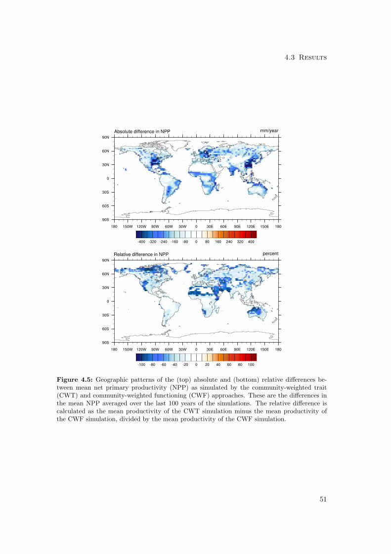
4.3 Results
Figure 4.5: Geographic patterns of the (top) absolute and (bottom) relative differences be-tween mean net primary productivity (NPP) as simulated by the community-weighted trait(CWT) and community-weighted functioning (CWF) approaches. These are the differences inthe mean NPP averaged over the last 100 years of the simulations. The relative difference iscalculated as the mean productivity of the CWT simulation minus the mean productivity ofthe CWF simulation, divided by the mean productivity of the CWF simulation.
51
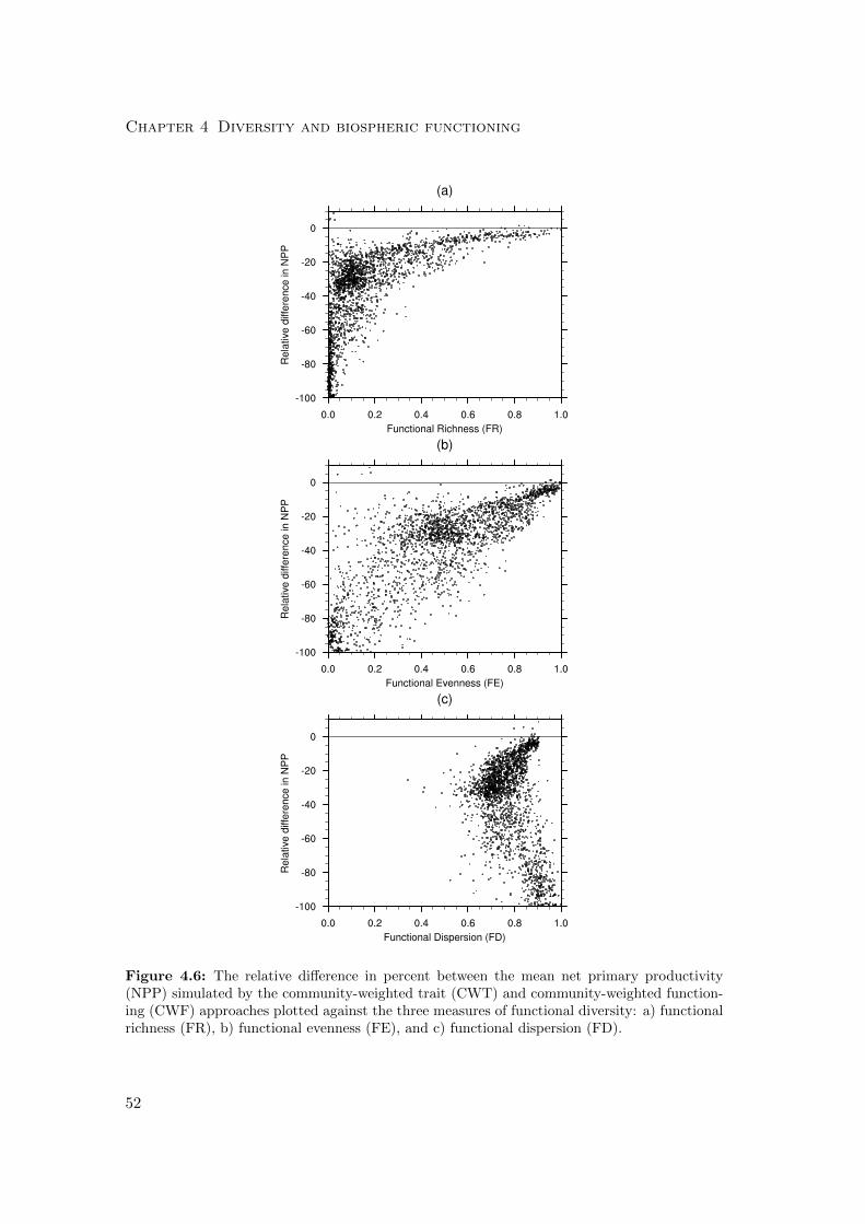
Chapter 4 Diversity and biospheric functioning
Figure 4.6: The relative difference in percent between the mean net primary productivity(NPP) simulated by the community-weighted trait (CWT) and community-weighted function-ing (CWF) approaches plotted against the three measures of functional diversity: a) functionalrichness (FR), b) functional evenness (FE), and c) functional dispersion (FD).
52
4.3 Results
are generally higher than in the CWF simulations. However, the strength of these
differences varies spatially and there are some regions where the ET flux is lower in the
CWT simulations. Also, the magnitude of these differences in relative terms, however,
is much less than for the NPP. For the ET fluxes, the patterns of absolute and relative
difference between the two simulations are quite similar. The absolute differences are
greatest in the tropics where the magnitude of the ET flux itself is highest. The greatest
absolute differences are generally in the tropical forests, especially the seasonal dry
forests of South America and southeast Asia, where the the land surface evapotranspires
more than 100 mm per year more in the CWT simulation than in the CWF simulation.
This corresponds to a relative increase of ET of about 10%. Larger relative differences
approaching 20% are found in the more temperate regions of western Europe, New
Zealand, and Chile.
The relationships between the relative differences in ET and the functional diversity
metrics (Fig. 4.8) are weaker and less clear than those for the relative differences in
NPP. There is a hump pattern in the relationships between the relative difference in
ET and the FR and FE diversity metrics, with low or negative relative differences
at the sites with the lowest FR and FE and the most pronounced relative difference
at intermediate richness and evenness, and again a reversion towards no change in ET
when approaching the grid cells with the highest FR and FE values. There is almost no
difference between the two approaches in the ET fluxes in the aseasonal and constantly
moist western Amazon basin, the region with the highest FR and FE values. Unlike
with NPP, the ET fluxes were also quite similar between the two approaches in regions
with the highest FD values.
4.3.2 Differences in variability of productivity and evapotranspiration
Fig. 4.9 shows the relative differences between the CWT and CWF simulation in the
interannual (top) and intraannual (bottom) variability of NPP. Fig. 4.10 shows the
same relative differences for the ET fluxes. The variability of the NPP and ET fluxes,
both interannual and intraannual, in the CWT simulation is generally higher than in
CWF simulation, although the spatial patterns vary between the the two fluxes and
the two measures of variability. There are no clear global relationships between the
relative differences in NPP or ET variability and the three functional diversity metrics.
The largest relative differences in the interannual variability of NPP (> 200% +) oc-
cur in the desert and arctic regions with high FD values, however, the temperate/boreal
forests and non-tropical grasslands also see strong positive relative differences. There
53
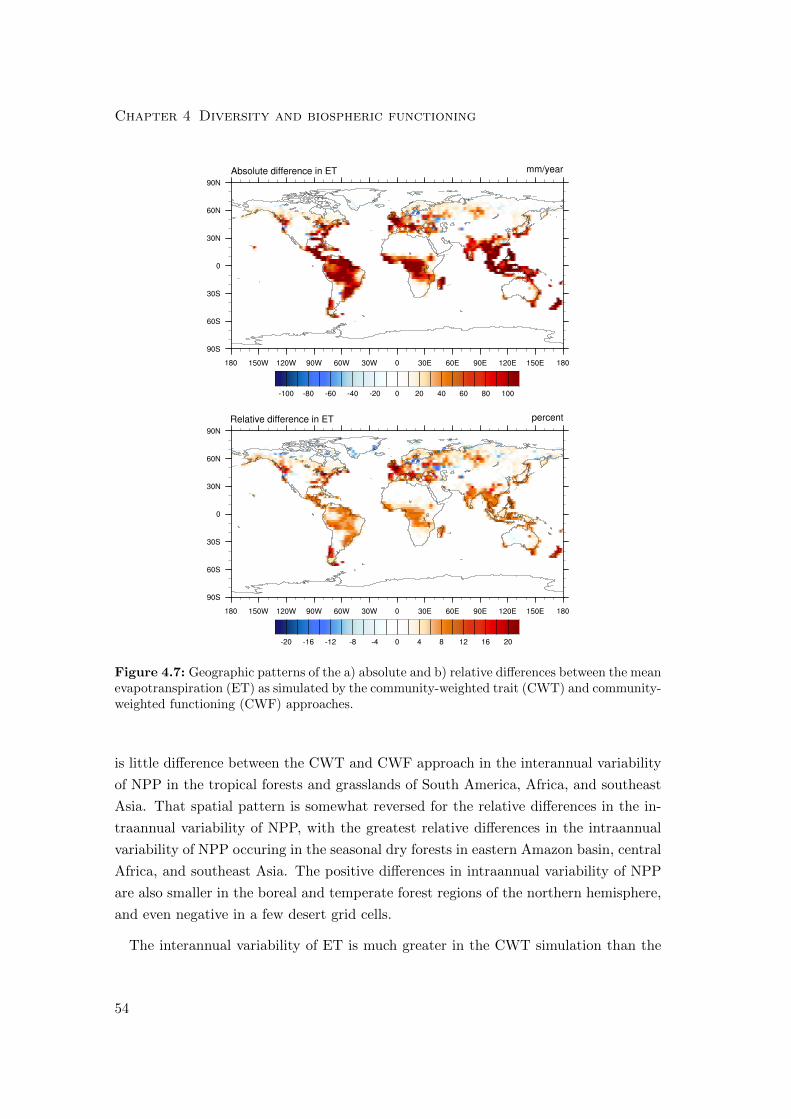
Chapter 4 Diversity and biospheric functioning
Figure 4.7: Geographic patterns of the a) absolute and b) relative differences between the meanevapotranspiration (ET) as simulated by the community-weighted trait (CWT) and community-weighted functioning (CWF) approaches.
is little difference between the CWT and CWF approach in the interannual variability
of NPP in the tropical forests and grasslands of South America, Africa, and southeast
Asia. That spatial pattern is somewhat reversed for the relative differences in the in-
traannual variability of NPP, with the greatest relative differences in the intraannual
variability of NPP occuring in the seasonal dry forests in eastern Amazon basin, central
Africa, and southeast Asia. The positive differences in intraannual variability of NPP
are also smaller in the boreal and temperate forest regions of the northern hemisphere,
and even negative in a few desert grid cells.
The interannual variability of ET is much greater in the CWT simulation than the
54
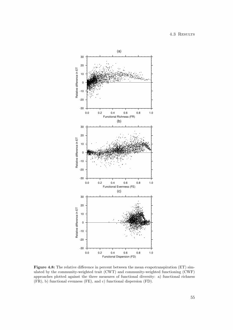
4.3 Results
Figure 4.8: The relative difference in percent between the mean evapotranspiration (ET) sim-ulated by the community-weighted trait (CWT) and community-weighted functioning (CWF)approaches plotted against the three measures of functional diversity: a) functional richness(FR), b) functional evenness (FE), and c) functional dispersion (FD).
55
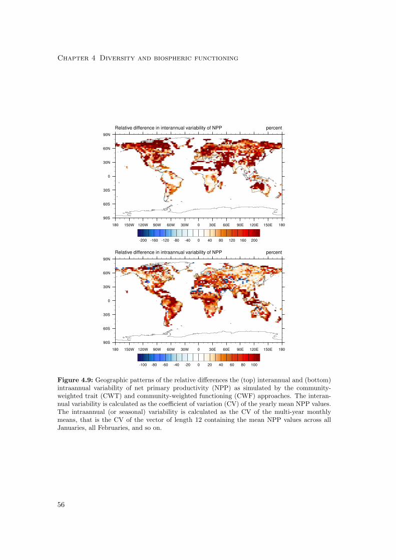
Chapter 4 Diversity and biospheric functioning
Figure 4.9: Geographic patterns of the relative differences the (top) interannual and (bottom)intraannual variability of net primary productivity (NPP) as simulated by the community-weighted trait (CWT) and community-weighted functioning (CWF) approaches. The interan-nual variability is calculated as the coefficient of variation (CV) of the yearly mean NPP values.The intraannual (or seasonal) variability is calculated as the CV of the multi-year monthlymeans, that is the CV of the vector of length 12 containing the mean NPP values across allJanuaries, all Februaries, and so on.
56
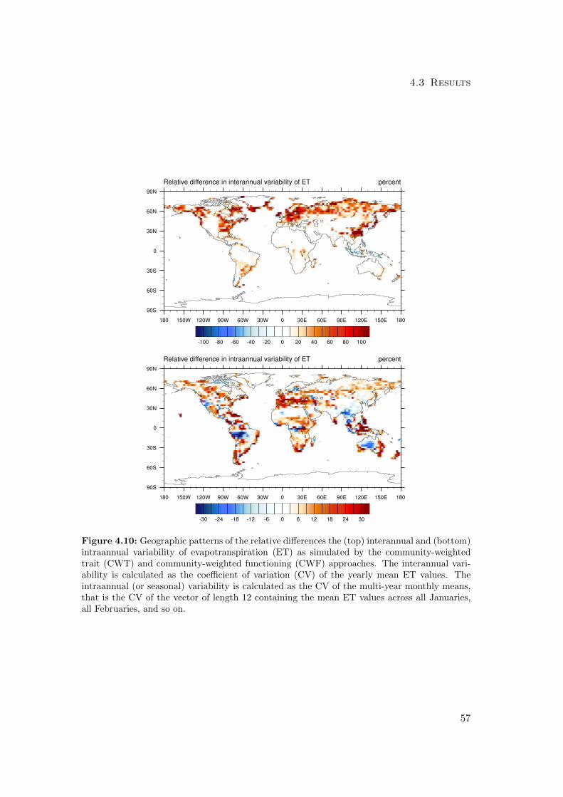
4.3 Results
Figure 4.10: Geographic patterns of the relative differences the (top) interannual and (bottom)intraannual variability of evapotranspiration (ET) as simulated by the community-weightedtrait (CWT) and community-weighted functioning (CWF) approaches. The interannual vari-ability is calculated as the coefficient of variation (CV) of the yearly mean ET values. Theintraannual (or seasonal) variability is calculated as the CV of the multi-year monthly means,that is the CV of the vector of length 12 containing the mean ET values across all Januaries,all Februaries, and so on.
57
Chapter 4 Diversity and biospheric functioning
CWF simulation throughout the temperate and boreal forest regions of North America
and Eurasia, more than 100% greater in some grid cells. There is little difference in
the interannual variability of ET in the tropics and arid region. The differences in
the intraannual variability of ET are more mixed. In some regions, e.g. around the
Mediterrean, the intraannual variability of ET is more than 25% greater in the CWT
simulation, while in other regions, e.g. the southern part of Amazon basin, it is 25%
less. There is no clear global trend relating the differences in the variability of ET and
any of the three functional diversity measures.
4.3.3 Differences in the resilience of the biosphere to climatic perturbation
Fig. 4.11 shows the simulated changes in global mean terrestrial NPP and ET over
the course of the first pertubation experiment in which the precipitation forcing was
reduced by 50%. . The changes shown are relative to the long-term means of each
flux prior to the imposing pertubation. Global mean NPP and ET fell significantly in
both the CWT and CWF simulations after reducing the precipitation. The simulated
fluxes associated with the diverse CWF simulation, however, were less affected by the
perturbation than the sparse CWT simulation. The NPP and ET fluxes decreased
across all regions (Fig. 4.13 and4.14, although the magnitude of these decreases varied
spatially. As one might expect, the semi-arid and arid regions showed the greatest
response to the reduction in precipitation in both simulations. The smallest changes
in both the CWT and CWF simulations are found in moist regions (e.g. tropical
rainforest, boreal forests).
Fig. 4.12 shows the simulated change in global mean terrestrial NPP over the course
of the second perturbation experiment in which a 2 degree warming was applied. Global
mean There was little difference between the two approaches in the global mean change
in ET after the warming pertubation. In the sparse PFT-like CWT simulation , the
warming resulted in lower NPP throughout the tropics (Fig. 4.15a) and mixed results
elsewhere. The diverse CWF simulation showed little change in NPP in the tropics
(Fig. 4.15b) and consistently positive changes throughout colder regions. The changes
in ET after the warming were relatively smaller (Fig. 4.16) than the changes in NPP
in both simulations.
58
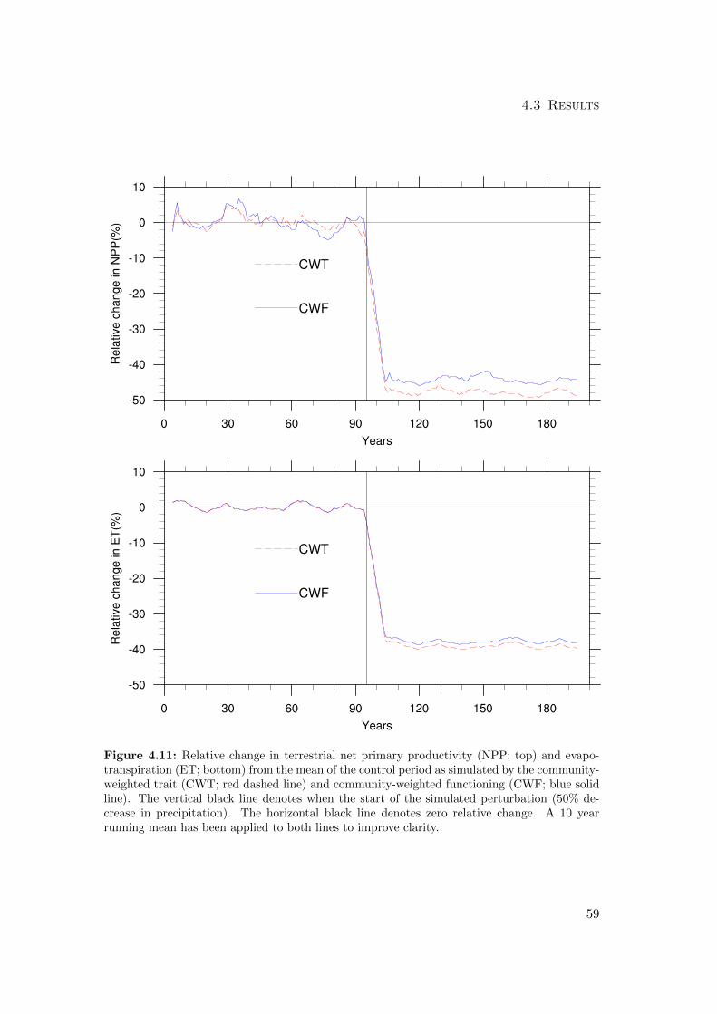
4.3 Results
Figure 4.11: Relative change in terrestrial net primary productivity (NPP; top) and evapo-transpiration (ET; bottom) from the mean of the control period as simulated by the community-weighted trait (CWT; red dashed line) and community-weighted functioning (CWF; blue solidline). The vertical black line denotes when the start of the simulated perturbation (50% de-crease in precipitation). The horizontal black line denotes zero relative change. A 10 yearrunning mean has been applied to both lines to improve clarity.
59
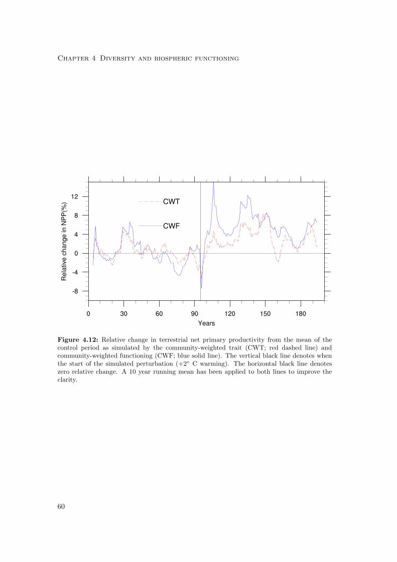
Chapter 4 Diversity and biospheric functioning
Figure 4.12: Relative change in terrestrial net primary productivity from the mean of thecontrol period as simulated by the community-weighted trait (CWT; red dashed line) andcommunity-weighted functioning (CWF; blue solid line). The vertical black line denotes whenthe start of the simulated perturbation (+2◦ C warming). The horizontal black line denoteszero relative change. A 10 year running mean has been applied to both lines to improve theclarity.
60
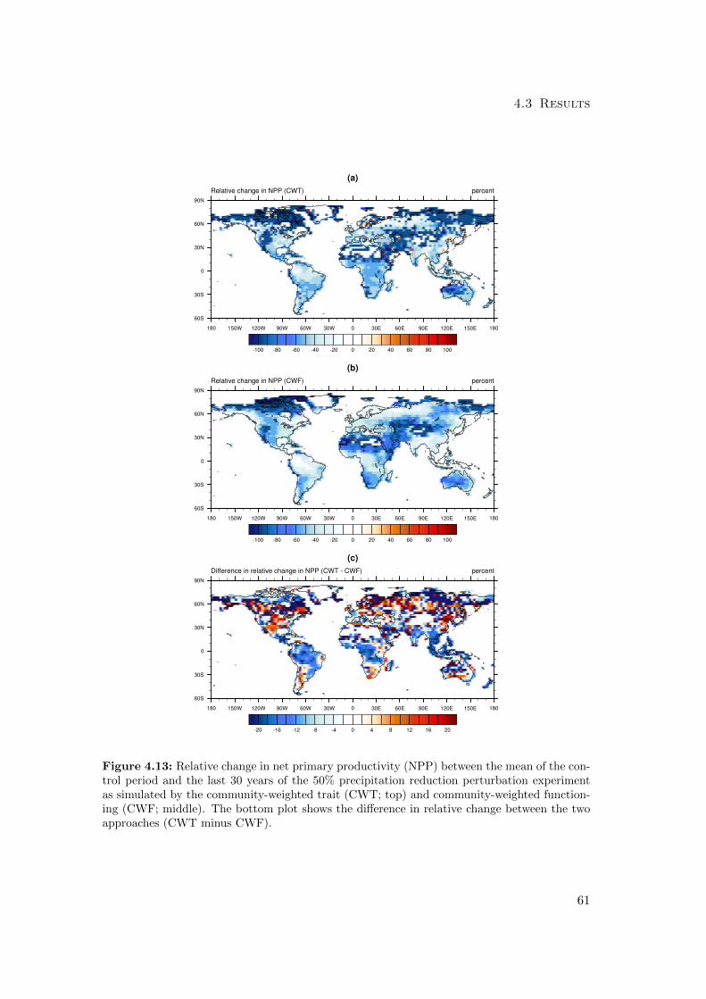
4.3 Results
Figure 4.13: Relative change in net primary productivity (NPP) between the mean of the con-trol period and the last 30 years of the 50% precipitation reduction perturbation experimentas simulated by the community-weighted trait (CWT; top) and community-weighted function-ing (CWF; middle). The bottom plot shows the difference in relative change between the twoapproaches (CWT minus CWF).
61
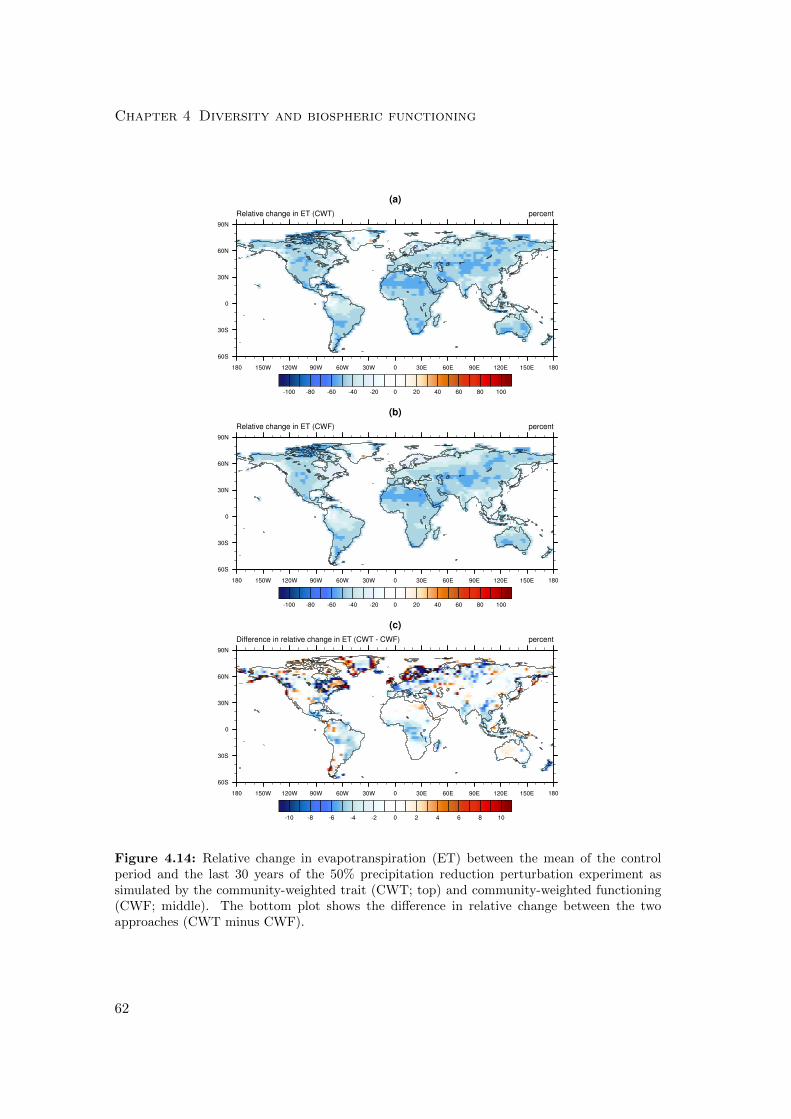
Chapter 4 Diversity and biospheric functioning
Figure 4.14: Relative change in evapotranspiration (ET) between the mean of the controlperiod and the last 30 years of the 50% precipitation reduction perturbation experiment assimulated by the community-weighted trait (CWT; top) and community-weighted functioning(CWF; middle). The bottom plot shows the difference in relative change between the twoapproaches (CWT minus CWF).
62
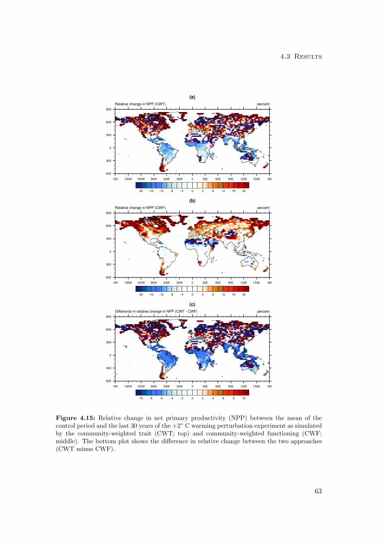
4.3 Results
Figure 4.15: Relative change in net primary productivity (NPP) between the mean of thecontrol period and the last 30 years of the +2◦ C warming perturbation experiment as simulatedby the community-weighted trait (CWT; top) and community-weighted functioning (CWF;middle). The bottom plot shows the difference in relative change between the two approaches(CWT minus CWF).
63
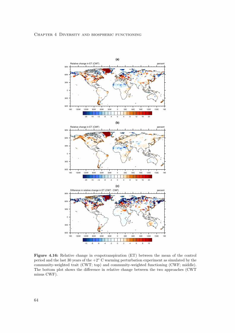
Chapter 4 Diversity and biospheric functioning
Figure 4.16: Relative change in evapotranspiration (ET) between the mean of the controlperiod and the last 30 years of the +2◦ C warming perturbation experiment as simulated by thecommunity-weighted trait (CWT; top) and community-weighted functioning (CWF; middle).The bottom plot shows the difference in relative change between the two approaches (CWTminus CWF).
64
4.4 Discussion
4.4 Discussion
This comparison of a diverse representation of functional diversity (CWF approach)
and coarse representation of functional diversity (CWT approach) yielded three major
results. The diverse approach resulted in (i) higher temporal mean vegetation produc-
tivity and water-use efficiency, (ii) a lower temporal variance of vegetation productivity
and evapotranspiration, and (iii) a more adaptive response to climatic perturbations
leading to more positive or less negative changes in productivity and evapotranspiration.
These insights are consistent with the ecological understanding of diversity-ecosystem
functioning relationships and are discussed in more detail in the following subsections.
4.4.1 Diversity-Productivity
The simulations showed that the diverse CWF approach yields higher temporal mean
productivity. This is consistent to what we hypothesized in the introduction of this
chapter (see Fig. 4.1). This effect of diversity on productivity is known as the diversity-
productivity hypothesis in ecological theory. This result of the JeDi-DGVM is surpris-
ing to some extent because the model does not account for faciliation, i.e. the beneficial
effects of one growth strategy on another.
We found that this productivity-enhancing effect was strongest in regions with the
highest FD. These are regions where the distribution of community biomass is dom-
inated by a few growth strategies which differ widely in one or more trait parameter
values. With a greater productivity, the diverse simulations also exhibited a greater
water-use efficiency (i.e. lower evapotranspiration flux relative to ecosystem productiv-
ity). This effect was strongest in tropical ecosystems. These results would imply that
the coarse representation of functional diversity in current PFT-based DGVMs may
lead to an underestimation of productivity and water-use efficiency.
4.4.2 Diversity-Variability
The simulations showed that the diverse CWF approach exhibits less temporal variation
in both productivity and evapotranspiration. This is the case for interannual variations
as well as seasonal variations within the year. This is again consistent to what we
hypothesized in the introduction and with previous diversity-manipulation experiments
(Tilman et al. 2006; Proulx et al. 2010; Allan et al. 2011) and models in theoretical
ecology (Tilman et al. 1998; Naeem 1998; Doak et al. 1998; Yachi 1999).
65
Chapter 4 Diversity and biospheric functioning
To some extent, these result are mathematically inevitable due to the averaging and
negative covariance effects. The growth strategy that does best in the mean climate,
can not necessarily be the most productive during drier or wetter years. In the con-
trary, species that do better during wet period, for instance by allocating more to leaf
growth can not also do better during dry periods, when possibly a higher allocation
to roots would be favorable. When growth strategies under altered conditions perform
better, they gain more biomass, becoming more abundant and consequently, more
heavily weighted in the aggregation of fluxes to the ecosystem-scale functioning. Thus,
with a richer represenation of functional diversity, the impact of climatic variability on
ecosystem functioning will be reduced.
The strong effect of the representation of diversity on the evapotranspiration is likely
to alter feedbacks between the vegetation and the atmosphere. The lower temporal
variability in fluxes associated with the diverse approach would seem likely to stabilize
vegetation fluxes under atmospheric variability, whereas the greater variability asso-
ciated with the CWT approach could amplify these effects. This result supports the
need for integrating a more diverse representation of functional diversity in to the land
surface component of Earth System models.
4.4.3 Diversity-Resilience
The productivity response of the diverse CWF simulation was generally less negative
than the CWT simulation to drying perturbation experiment. The CWF simulation
also exhibited generally more positive changes in productivity in response to the warm-
ing perturbation experiment. On the other hand, in the CWT simulation, the produc-
tivity decreased dramatically in some regions. This outcome is expected because the
diverse representation allows for a shift in the dominance towards growth strategies
with traits more suited to the altered conditions. This is also consistent with other
two results described above. In a way this is the same result as the case of diversity-
productivity effect, except that climatic variability is replaced by a climatic change.
This insight is specifically relevant for climate change research. For instance, the
study by Cox et al. (2000) suggest an Amazon dieback under global warming scenar-
ios. This result was obtained with a coarse representation of functional diversity with
only a very few PFTs. Our results imply that with a more diverse representation of
vegetation within an Earth system model would lead to less severe vegetation changes
under climatic change. This would also support the importance of conserving func-
tional diversity in ecosystems for them to maintain their ability to adapt to changing
66
4.5 Summary of diversity-biospheric functioning relationships
conditions.
4.5 Summary of diversity-biospheric functioning relationships
JeDi-DGVM simulations were run in two configurations to quantify how the representa-
tion of functional diversity influences the simulated magnitude and variability of water
and carbon fluxes between the land surface and the atmosphere. In the first configura-
tion, we simulated a diverse biosphere using a large number of plant growth strategies,
allowing the modelled ecosystems to adapt through emergent changes in ecosystem
composition. In the second configuration, we recreated a low diversity PFT-like rep-
resentation of the terrestrial biosphere by aggregating the surviving growth strategies
from the diverse simulation to a single community-weighted plant growth strategy per
grid cell. In agreement with earlier biodiversity-ecosystem functioning studies, the di-
verse representation of terrestrial vegetation exhibited higher productivity and water-
use efficiency in many regions. The land surface fluxes of productivity in the diverse
simulations show greater temporal stability and resilience to climatic perturbations.
The strength of these differences in magnitude and variability were modulated by the
composition of the simulated ecosystems in the diverse simulations. In summary, these
results support the notion that functional diversity plays a role in the functioning of
the Earth System.
These results demonstrate a need for improving the representation of functional diver-
sity in comprehensive Earth System models and add support for conserving biodiversity
to maintain ecosystem services and land surface functioning.
67

Chapter 5
Summary and outlook
5.1 Summary
In this thesis, we introduced JeDi-DGVM as a prototype for a new class of dynamic
global vegetation models with representation of functional diversity that are less coarse
and less reliant on empirical bioclimatic relationships than previous PFT-based ap-
proaches. This is accomplished with (i) a mechanistic representation of functional
trade-offs, which (ii) constrain a large number of plant growth strategies with trait pa-
rameter values randomly sampled from their complete theoretical/observed ranges, and
(iii) the aggregation of the fluxes/properties associated with those growth strategies to
grid-scale structure and function based on their relative abundances.
In a systematic evaluation of JeDi-DGVM in Chapter 3, we have shown that its
bottom-up plant functional tradeoff approach together with a simple mass-based ag-
gregation mechanism is able to capture the broad patterns of terrestrial biogeochemical
fluxes and associated land surface properties reasonably well. The evaluation results
compare favorably with two other state-of-the-art terrestrial biosphere models based
on the presently dominant PFT paradigm. Additionally, we have shown that JeDi-
DGVM is able to mechanistically reproduce the global-scale biogeographical patterns
of plant species richness and community evenness. Because it is more closely based on
first-principles, JeDi-DGVM requires less input data and is able to produce a wider
range of testable outputs than earlier DGVMs based on the PFT concept.
We have also shown in Chapter 4, that when compared with a coarser representation
of functional diversity, that the diverse JeDi-DGVM approach leads to a simulated
terrestrial biosphere with higher productivity and water-use efficiency, greater stability
in terms of its carbon and water fluxes, and greater resilience to climatic perturba-
tions. These findings fit with previous theoretical and empirical work on biodiversity-
69
Chapter 5 Summary and outlook
ecosystem functioning relationships. They highlight the need for improving the rep-
resentation of functional diversity within the vegetation component of comprehensive
Earth System models, but they also bolster support for conserving biodiversity to
maintain biospheric functioning in a changing climate.
The JeDi-DGVM modelling approach developed in this thesis sets the foundation
for future applications, in which the simulated vegetation response to global change
has a greater ability to adapt through changes in ecosystem composition, having po-
tentially wide-ranging implications for biosphere-atmosphere interactions under global
change. In the next and last section of this thesis, we propose possible directions for
further model development/evaluation and we highlight a few ongoing and potential
applications of JeDi-DGVM.
5.2 Outlook
JeDi-DGVM introduces several elements novel to dynamic vegetation modeling, allow-
ing for an explicit representation of functional diversity that can evolve temporally. As
the current implementation represents an initial prototype from which refinements and
added functionality will be made, we discuss below several key concepts that underlie
the formulation of JeDi-DGVM, and which will likely result in the greatest impact on
model improvement in future efforts. We also highlight several ongoing and potential
applications of the model.
5.2.1 Representation of tradeoffs
JeDi-DGVM is a prototype meant to explore the potential utility of a trait-based
functional tradeoff approach for transitioning the state-of-the-art of global vegetation
modelling beyond the limitations of a set of fixed PFTs. One of the greatest potential
advantages of this approach is that it does not constrain the vegetated land surface
to be represented by a small set of functional types, but instead allows for a more
continuous representation of vegetation types that can evolve as a function of climatic
suitability. We demonstrate in this work that from this tradeoff-based approach a
realistic representation of land surface biophysical form and function can emerge.
For this approach to be successful, several key requirements must be met, particularly
(1) identification of the key tradeoffs that determine the ability of a plant to survive
in a given environment, and (2) proper parameterization of the costs and benefits of
70
5.2 Outlook
the traits associated with those tradeoffs. In this current implementation, JeDi-DGVM
utilizes 15 functional parameters that characterize the behavior of a growth strategy
in terms of its carbon allocation strategy, phenological dynamics, tissue turnover and
the balance between respiration and photosynthesis. The positive performance of JeDi-
DGVM in the C-LAMP evaluation lends credibility to this approach, and will motivate
further evaluation of the critical plant traits and tradeoffs that determine the perfor-
mance of the vegetated land surface. New information sources linking costs and benefits
with observed traits, such as the TRY database (Kattge et al. 2011), will provide im-
portant constraints on future refinements of this approach.
5.2.2 Is everything everywhere?
JeDi-DGVM assumes that the distribution of plant growth strategies is able to ad-
just quickly to climatic changes, allowing all of the sampled plant growth strategies
to emerge when a given climate anywhere on the globe becomes suitable. This can be
stated through the ecological hypothesis of “Everything is everywhere, but the environ-
ment selects.” While this ecological hypothesis was originally formulated with respect
to the biogeography of marine microbes, terrestrial plant species face considerable bar-
riers to migration (e.g. mountain ranges, deserts, oceans). The timescales of terrestrial
plant growth and dispersal also differ greatly from those of fast-lived marine microbes
transported along ocean currents. A model-based study (Malcolm et al. 2002) showed
that the preferred ranges of many plant species could shift tens to hundreds of kilome-
ters over the next century due to anthropogenic greenhouse warming, making the issue
of estimating migration rates, and the extent to which everything is truly everywhere,
key to predicting future vegetation composition.
Despite the importance of this issue to the vegetation modelling community (Neilson
et al. 2005), only one modelling group (Lee 2011) has introduced mechanistic migration
processes in a DGVM. Lee (2011) attributes this partially to the difficulties associated
with the considerable variation in seed dispersal rates within the PFTs used by the
current generation of DGVMs. Incorporating aspects of seed dispersal in a functional
tradeoff framework, through additional traits such as seed size, could help to constrain
plant migration rates in climate change simulation experiments. Seed dispersal range,
and consequently the rate of plant migration, is closely linked to seed size. Smaller seeds
are more easily transported by the wind and animals than larger seeds (Ezoe 1998). On
the other hand, larger seeds allow establishing plants to persist through longer periods
of stress. Parameterizing the tradeoff between seed size and dispersal rates will be
71
Chapter 5 Summary and outlook
challenging but possibly less so than modelling migration with a PFT-based scheme.
5.2.3 Aggregation scheme and competition
The aggregation of vegetation states and fluxes across the diversity represented in
each computational grid cell is based on the ‘biomass-ratio’ hypothesis. This scheme
determines the grid cell flux or state as an average across all surviving plant growth
strategies in the grid cell, weighted by their respective biomass, imposing the implicit
assumption that interaction between plant growth strategies is weak. For example,
JeDi-DGVM does not currently account for shading of plant growth strategies that
resemble understory plants by those that resemble dominant canopy trees. Likewise,
the hydrologic conditions that a plant growth strategy experiences are not influenced
by the other surviving plant growth strategies in its grid cell. Thus, understory plant
growth strategies do not stand to benefit during periods of drought from the observed
phenomena of hydraulic distribution, wherein deep-rooted plants redistribute soil water
from lower soil layers (Lee et al. 2005; Prieto et al. 2012). These types of competitive
and facilitative interactions are known to influence community-assembly processes at
the local scale (Cavender-Bares et al. 2009), leading to trait divergence. However, at
larger scales, including the spatial resolution of the simulation results presented here,
trait selection and trait convergence due to environmental filtering have been shown to
be the dominant community-assembly processes (Kraft et al. 2008; Swenson and Weiser
2010; Freschet et al. 2011; Kraft et al. 2011).
This ‘biomass-ratio’ aggregation scheme was chosen for its simplicity and its demon-
strated effectiveness for making statistical predictions about community fluxes from
trait abundance information at the field-scale (Garnier et al. 2004; Vile et al. 2006;
Kazakou et al. 2006; Dıaz et al. 2007; Quetier et al. 2007). However, the mechanistic
tradeoff-based trait filtering framework of JeDi-DGVM does not preclude the inte-
gration of more sophisticated aggregation schemes. For example, Bohn et al. (2011)
recently used JeDi-DGVM model output together with a simple population dynamics
model DIVE (Dynamics and Interactions of VEgetation) to explore how seed competi-
tion, resource competition and environmental disturbance might influence community
structure. In the future, the tradeoff-based modelling approach of the JeDi-DGVM
could be directly integrated with the representation of population dynamics from the
DIVE model or from other recent models (e.g. the Ecosystem Demography model;
Moorcroft et al. 2001; Medvigy et al. 2009; Fisher et al. 2010b) which explicitly ac-
count for canopy height structure and age classes.
72
5.2 Outlook
5.2.4 Further evaluation
In this thesis, we evaluated the feasibility of using the JeDi-DGVM modelling approach
to simulate broad-scale patterns of terrestrial biogeochemistry and ecosystem proper-
ties. However, another key and unique test for this approach would be to directly com-
pare the emergent patterns of simulated FT parameters with our growing knowledge
about the geographic distribution of plant traits and their environmental co-variates.
This information could come from trait databases (e.g. TRY; Kattge et al. 2011) or
remote sensing products (e.g. canopy nitrogen observations; Ollinger et al. 2008). A
further test would be to compare simulated shifts in FT parameters and allocation
patterns with observed shifts in trait abundances from ecosystem manipulation exper-
iments, e.g. irrigation (Axelsson and Axelsson 1986), CO2 enhancement (Ainsworth
and Long 2004), or throughfall exclusion (Fisher et al. 2007). These fine-scale compar-
isons would help further refine various aspects of the biogeochemical formulations and
trade-offs incorporated into JeDi-DGVM, and give greater confidence in projections
regarding the future fate of the terrestrial biosphere.
In Chapter 3.4.10, we briefly compared the simulated allocation of NPP to differ-
ent plant carbon pools with carbon budget observations (Malhi et al. 2009) from three
Amazonian forest ecosystems. This analysis should be expanded globally by comparing
the the simulated patterns of carbon flows and stocks with observations from other ex-
isting datasets based on carbon inventories (Cannell 1982; Litton et al. 2007; Luyssaert
et al. 2007; Malhi et al. 2011). More specifically, one could look at how the simu-
lated allocation patterns vary along environmental gradients (cf. Litton and Giardina
2008; Cornwell and Ackerly 2009). In this study we only examined at the community-
weighted allocation fluxes. It would be equally interesting to explore how the simulated
partitioning of NPP varies among surviving plant growth strategies within grid cells
(cf. Ackerly and Cornwell 2007).
For instance, Wolf et al. (2011) and Malhi et al. (2011) found evidence that the
strongest allocation trade-off was not between root and shoots, as has been commonly
thought, but rather more specifically between allocation to fine roots and aboveground
wood. This relationship is likely mediated between sites by hydrological conditions and
within sites by the competitive dynamics between faster and slower growing trees. In
principle, the functional tradeoff modelling approach of JeDi-DGVM should be able to
capture both of these phenomena. However, it might require the introduction of further
constraints related to disturbances (Bohn et al. 2011) and FT parameters related to
wood economics and plant hydraulics (cf. Hickler et al. 2006; Chave et al. 2009; Falster
73
Chapter 5 Summary and outlook
et al. 2010)
5.2.5 Ongoing and potential applications
The “bottom-up” functional tradeoff-based modelling framework presented here repre-
sents a step forward in the development of a comprehensive and predictive representa-
tion of the terrestrial biosphere for use in Earth System Models. By mechanistically
simulating the full range and continuous nature of plant functional diversity, it will be
possible to explore new areas of research including:
1. The JeDi-DGVM is currently participating in the Intersectoral Model Intercom-
parison Project. This initiative is seeking to make quantitative estimates regard-
ing climate change impacts and their uncertainties across different sectors (e.g.
agriculture, water, ecosystems, infrastructure and health) with multiple impact
models. We hypothesize based on the results from Chapter 4, which showed
the more flexible approach of JeDi led to greater productivity, stability, and re-
silience than a more coarse PFT-like represenation of functional diversity, that
JeDi-DGVM will simulate less severe biospheric impacts of projected climate
change than the other participating DGVMs based on the PFT paradigm.
2. By coupling the JeDi-DGVM tradeoff-based approach with an optimization algo-
rithm, it is possible to seek out those functional trait combinations that maximize
a particular ecosystem service. For example, Drewry et al. (in prep), have used
JeDi-DGVM to investigate the the optimal set of trait parameters which maxi-
mize the allocation to seed biomass under the present-day climate of each model
grid cell, allowing for estimates of the upper bound of realizable yields as a func-
tion of climatic constraint. One could also apply the same methodology with
climate model projections to identify regions where the optimal crop traits shift
in order to inform agricultural and food security policies. The same methodology
could also easily be applied to many other ecosystem system services of inter-
est (e.g. maximizing leaf biomass production for forage/fodder or belowground
carbon allocation for carbon sequestration).
3. Climate model projections point towards the possibility of novel climates without
present-day analogs (Jackson and Williams 2004; Williams and Jackson 2007).
This causes difficulties for PFT-based modelling approaches because they often
rely so heavily on bioclimatic relationships based on present-day empirical ob-
servations. Because JeDi-DGVM samples functional trait parameters from their
74
5.2 Outlook
full theoretical or observed ranges, it may produce surviving growth strategies
or compositions of growth strategies without present-day analogs (Reu et al., in
review). Coupling JeDi-DGVM directly within an Earth System Model would
allow for the exciting possibility of exploring where these no-analog vegetation
compositions appear in climates that widely different from that of today. It
would also be interesting to explore the role of functional diversity in moderat-
ing atmosphere-biosphere feedbacks. As an example, one could compare “online”
and “offline” simulations to quantify the net effect of biodiversity on sustaining
continental moisture recycling.
75

Appendix A
Jena Diversity-Dynamic Global Vegetation
(JeDi-DGVM) Model Description
JeDi-DGVM builds upon the plant diversity model of KM2000, which itself took many
model formulations from earlier land surface (Roeckner et al. 1996) and terrestrial bio-
sphere models (e.g. Potter et al. 1993; Knorr and Heimann 1995; Kaduk and Heimann
1996). Here, the ecophysiological parameterizations have been kept relatively simple to
keep the computational requirements manageable. This makes it possible to simulate
many the development of many plant growth strategies in parallel across a global grid
over long simulation periods within a reasonable timeframe on a single Linux worksta-
tion. That said, several of the formulations and parameter values, particularly with
respect to the calculation of productivity and respiration, have been changed to im-
prove the realism of the simulated fluxes. Also, whereas the KM2000 model simulated
the life-cycle of individual generic plants from germination to death, the JeDi-DGVM
introduces tissue turnover and thus simulates something closer to the mean of a pop-
ulation for each plant growth strategy. Finally, the most important new feature is
the introduction of a scaling mechanism to aggregate the exchange fluxes and land-
surface properties of many plant growth strategies to the community-level based on the
‘biomass-ratio’ hypothesis.
A.1 Plant module overview
The plant module simulates the development of plant growth strategies based on the
fundamental ecophysiological processes of photosynthesis, respiration, allocation, phe-
nology, and reproduction. Plant development is coupled in a process-based manner
to a land-surface hydrology module which simulates canopy interception, throughfall,
infiltration, evaporation, root-water uptake, and surface runoff, using daily meteoro-
77
Appendix A Model Description
logical forcing of downwelling shortwave and net longwave radiation, precipitation, and
near-surface air temperature. The variables and parameters involved in the develop-
ment of the plant growth strategies are summarized in Table C.1. The details of the
land-surface module are described in Appendix B.
Each plant growth strategy is represented by six carbon tissue pools: stored assim-
ilates CA, leaves CL, fine roots CR, aboveground wood (branches and stems) CWL,
belowground wood (coarse roots) CWR, and a reproductive (or ‘seed’) pool CS. When
growing conditions are favorable, carbon germinates from the ‘seed’ pool to the storage
pool. The plant then begins to grow by allocating carbon from the storage pool to
the various tissue pools. The tissue pools are also subject to turnover and senescence.
The litter fluxes from these two processes serve as input to the soil carbon module.
The sizes of the tissue pools influence the parameter values of the land-surface module,
affecting both the absorption of solar radiation and the land-surface hydrology. For ex-
ample, the absorption of solar radiation, which supplies the energy for photosynthesis
and evapotranspiration, is proportional to leaf area index (LAI) which is derived from
leaf biomass. Fine root biomass affects the maximum rate of water uptake from the
rooting zone, influencing the plant’s water status and the supply of moisture for evap-
otranspiration. Likewise, the coarse root biomass of a plant determines the hydrologic
depth of its rooting zone. The land-surface conditions in turn affect the net primary
productivity (NPP), which forms the input to the storage pool. A plant growth strat-
egy is considered to be alive as long as the carbon in the storage pool is greater than
zero (CA > 0). The details of these processes are described in the following subsections.
The particular functioning of a plant growth strategy is defined by a set of 15 func-
tional trait (FT) parameters (t1 ... t15). These FT parameters control the allocation
of carbon from the storage pool to the other tissue pools, the tissue turnover rates, the
phenological response to environmental conditions, and the ecophysiological balance
between photosynthesis and respiration. All of the FT parameters range between zero
and one. However, these ranges are often extended by using the FT parameters as
either exponents or coefficients. Each FT parameter is associated with one or more
functional tradeoffs. For instance, a higher allocation to fine roots enhances the rate at
which a plant can extract moisture from the soil matrix, but this comes at the expense
of allocation to the aboveground pools and thus a decreased ability to capture light for
photosynthesis, as well as the metabolic cost of maintaining that biomass. The imple-
mentation of these tradeoffs are explained in further detail below. The descriptions of
the FT parameters are summarized in Table C.2.
78
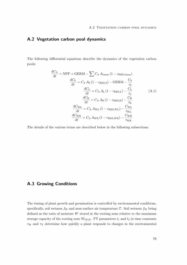
A.2 Vegetation carbon pool dynamics
A.2 Vegetation carbon pool dynamics
The following differential equations describe the dynamics of the vegetation carbon
pools:
dCA
dt= NPP + GERM−
∑CAAtissue (1− cRES,tissue)
dCS
dt= CAAS (1− cRES,S)−GERM− CS
τS
dCL
dt= CAAL (1− cRES,L)− CL
τL(A.1)
dCR
dt= CAAR (1− cRES,R)− CR
τR
dCWL
dt= CAAWL (1− cRES,WL)− CWL
τWL
dCWR
dt= CAAWR (1− cRES,WR)− CWR
τWR
The details of the various terms are described below in the following subsections.
A.3 Growing Conditions
The timing of plant growth and germination is controlled by environmental conditions,
specifically, soil wetness fW and near-surface air temperature T . Soil wetness fW being
defined as the ratio of moisture W stored in the rooting zone relative to the maximum
storage capacity of the rooting zone WMAX. FT parameters t1 and t2 in time constants
τW and τT determine how quickly a plant responds to changes in the environmental
79
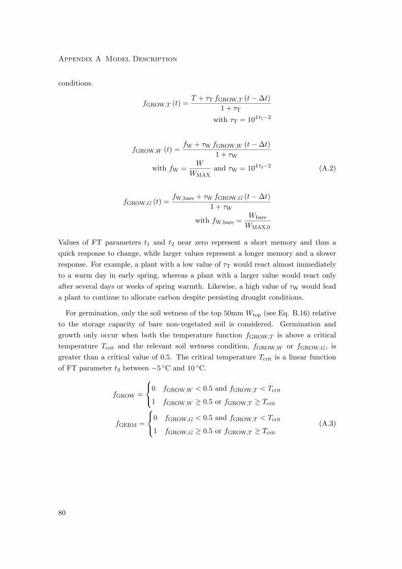
Appendix A Model Description
conditions.
fGROW,T (t) =T + τT fGROW,T (t−∆t)
1 + τT
with τT = 104 t1−2
fGROW,W (t) =fW + τW fGROW,W (t−∆t)
1 + τW
with fW =W
WMAXand τW = 104 t2−2 (A.2)
fGROW,G (t) =fW,bare + τW fGROW,G (t−∆t)
1 + τW
with fW,bare =Wbare
WMAX,0
Values of FT parameters t1 and t2 near zero represent a short memory and thus a
quick response to change, while larger values represent a longer memory and a slower
response. For example, a plant with a low value of τT would react almost immediately
to a warm day in early spring, whereas a plant with a larger value would react only
after several days or weeks of spring warmth. Likewise, a high value of τW would lead
a plant to continue to allocate carbon despite persisting drought conditions.
For germination, only the soil wetness of the top 50mm Wtop (see Eq. B.16) relative
to the storage capacity of bare non-vegetated soil is considered. Germination and
growth only occur when both the temperature function fGROW,T is above a critical
temperature Tcrit and the relevant soil wetness condition, fGROW,W or fGROW,G, is
greater than a critical value of 0.5. The critical temperature Tcrit is a linear function
of FT parameter t3 between −5 ◦C and 10 ◦C.
fGROW =
0 fGROW,W < 0.5 and fGROW,T < Tcrit
1 fGROW,W ≥ 0.5 or fGROW,T ≥ Tcrit
fGERM =
0 fGROW,G < 0.5 and fGROW,T < Tcrit
1 fGROW,G ≥ 0.5 or fGROW,T ≥ Tcrit
(A.3)
80
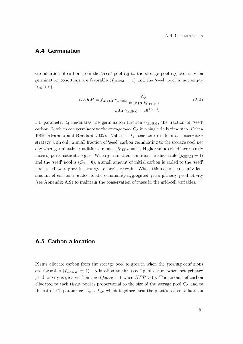
A.4 Germination
A.4 Germination
Germination of carbon from the ‘seed’ pool CS to the storage pool CA occurs when
germination conditions are favorable (fGERM = 1) and the ‘seed’ pool is not empty
(CS > 0):
GERM = fGERM γGERMCS
max (p, kGERM)(A.4)
with γGERM = 104 t4−4.
FT parameter t4 modulates the germination fraction γGERM, the fraction of ‘seed’
carbon CS which can germinate to the storage pool CA in a single daily time step (Cohen
1968; Alvarado and Bradford 2002). Values of t4 near zero result in a conservative
strategy with only a small fraction of ‘seed’ carbon germinating to the storage pool per
day when germination conditions are met (fGERM = 1). Higher values yield increasingly
more opportunistic strategies. When germination conditions are favorable (fGERM = 1)
and the ‘seed’ pool is (CS = 0), a small amount of initial carbon is added to the ‘seed’
pool to allow a growth strategy to begin growth. When this occurs, an equivalent
amount of carbon is added to the community-aggregated gross primary productivity
(see Appendix A.9) to maintain the conservation of mass in the grid-cell variables.
A.5 Carbon allocation
Plants allocate carbon from the storage pool to growth when the growing conditions
are favorable (fGROW = 1). Allocation to the ‘seed’ pool occurs when net primary
productivity is greater then zero (fSEED = 1 when NPP > 0). The amount of carbon
allocated to each tissue pool is proportional to the size of the storage pool CA and to
the set of FT parameters, t5 . . . t10, which together form the plant’s carbon allocation
81
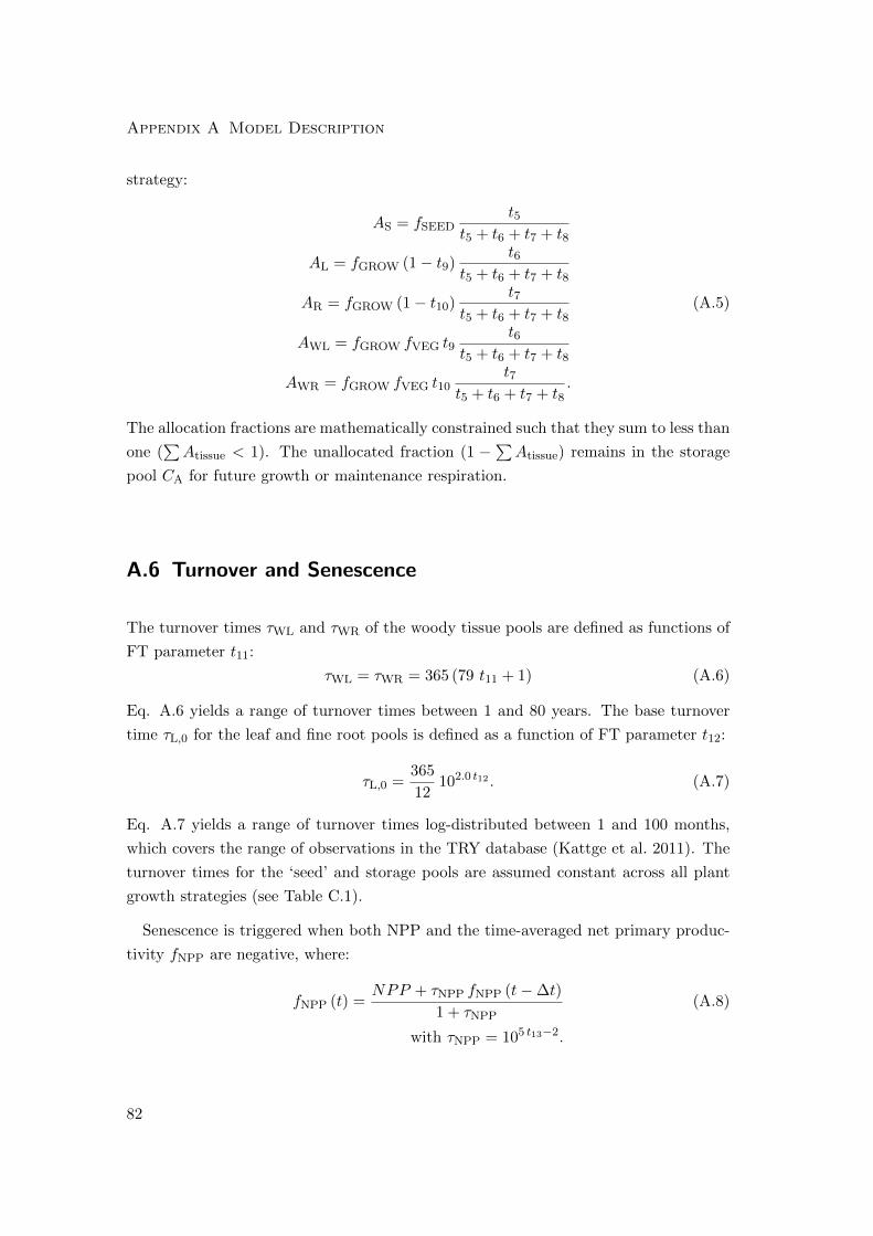
Appendix A Model Description
strategy:
AS = fSEEDt5
t5 + t6 + t7 + t8
AL = fGROW (1− t9)t6
t5 + t6 + t7 + t8
AR = fGROW (1− t10)t7
t5 + t6 + t7 + t8(A.5)
AWL = fGROW fVEG t9t6
t5 + t6 + t7 + t8
AWR = fGROW fVEG t10t7
t5 + t6 + t7 + t8.
The allocation fractions are mathematically constrained such that they sum to less than
one (∑Atissue < 1). The unallocated fraction (1 −
∑Atissue) remains in the storage
pool CA for future growth or maintenance respiration.
A.6 Turnover and Senescence
The turnover times τWL and τWR of the woody tissue pools are defined as functions of
FT parameter t11:
τWL = τWR = 365 (79 t11 + 1) (A.6)
Eq. A.6 yields a range of turnover times between 1 and 80 years. The base turnover
time τL,0 for the leaf and fine root pools is defined as a function of FT parameter t12:
τL,0 =365
12102.0 t12 . (A.7)
Eq. A.7 yields a range of turnover times log-distributed between 1 and 100 months,
which covers the range of observations in the TRY database (Kattge et al. 2011). The
turnover times for the ‘seed’ and storage pools are assumed constant across all plant
growth strategies (see Table C.1).
Senescence is triggered when both NPP and the time-averaged net primary produc-
tivity fNPP are negative, where:
fNPP (t) =NPP + τNPP fNPP (t−∆t)
1 + τNPP(A.8)
with τNPP = 105 t13−2.
82
A.7 Land Surface Parameters
fSEN =
0 fNPP ≥ 0 or NPP ≥ 0
1 fNPP < 0 and NPP < 0(A.9)
FT parameter t13 in time constant τNPP describes the memory to past NPP conditions.
Values of t13 near zero represent a short persistence during periods of negative NPP,
while values closer to one represent longer persistence. During periods of senescence,
the turnover rates of the leaf and fine root pools increase proportional to a constant
factor τSEN. The relative magnitude of this increase is determined by FT parameter
t14:
τL =
(1
τL,0+
1
τSENfSEN t14
)−1
τR =
(1
τL,0+
1
τSENfSEN (1− t14)
)−1
(A.10)
A.7 Land Surface Parameters
The land-surface parameters (maximum plant available water storage in the rooting
zone WMAX, leaf area index LAI, potential supply rate for transpiration S, fractional
vegetative cover fVEG, fractional forest cover fFOR, snow-free surface albedo ans, and
the storage capacity of the canopy WLMAX) relate the development of a plant growth
strategy to the coupled land-surface module which simulates its environmental con-
ditions. The module itself is based on the land-surface component of the ECHAM4
atmospheric General Circulation Model (Roeckner et al. 1996) along with modifica-
tions introduced by KM2000 and is described in detail in Appendix B. These parame-
ters are computed for each plant growth strategy from its carbon tissue pools and FT
parameters:
LAI = CL SLA
fVEG = 1− e−k LAI
fFOR = 1− e−cFOR CWL
WLMAX = cWLMAX LAI (A.11)
ans = fVEG aVEG + (1− fVEG) aSOIL
Wmax = max[Wmax,0, cPAW
√cSRLCWR
]S = cSRUCR fW
83
Appendix A Model Description
The land-surface parameters and their conversion constants are summarized in Table
C.3.
The leaf area index LAI of a plant growth strategy is calculated as the product of
its leaf biomass CL and its specific leaf area SLA. The SLA of a plant growth strategy
being estimated as a function of leaf lifespan using an empirical relationship derived by
Reich et al. (1997), where τL0 is the base leaf turnover rate from Eq. A.7.
SLA = 0.030
(365
τL0
)−0.46
(A.12)
This establishes a trade-off such that a plant growth strategy falls along a spectrum
between an evergreen strategy with thicker, long-lived leaves and a deciduous strategy
with thinner, short-lived leaves (Reich et al. 1998; Westoby et al. 2002; Shipley et al.
2006a).
The leaf area index LAI is then used to determine both the fractional vegetation
cover fVEG according to the Lambert-Beer law (Monsi and Saeki 1953) and the water
storage capacity of the canopy WLMAX . The parameterization of the fractional forest
cover fFOR is taken as an analogy to the formulation used for vegetative cover fVEG.
The snow-free surface albedo ans is calculated as the mean of its canopy albedo aVEG
and the bare soil albedo aSOIL (constant for all plant growth strategies), weighted by its
fractional vegetation cover fVEG. The canopy albedo aVEG of a plant growth strategy
is a linear function of the canopy nitrogen concentration [NL] (Hollinger et al. 2010).
aVEG = 3.216 [NL] + 0.02 (A.13)
The formulations regarding root properties (WMAX and S) are obtained from first
principles. The motivation for using a square-root relationship for the maximum plant
available water storage in the rooting zone comes from the Shinozaki et al. (1964) pipe
model. From the pipe model perspective, the root system is viewed as an assemblage
of pipes which connect the root ends (the organs responsible for water absorption from
the soil) with the leaves. If we assume a uniform density of root ends within the
rooting zone, we obtain a square root relationship between the depth of the rooting
zone and the total length of the coarse roots (given by the product of the coarse root
biomass CWR and an assumed constant specific root length parameter cSRL). The
maximum plant available soil water storage WMAX is then given by the product of this
rooting zone depth and the unit plant available water capacity cPAW (i.e. the difference
between field capacity and permanent wilting point per unit depth) taken from a global
84
A.8 Net Primary Productivity
dataset (Dunne and Willmott 1996). Finally, we assume the potential supply rate for
transpiration S is related to the fine root biomass CR and soil wetness fW via a constant
specific root water uptake parameter cSRU.
A.8 Net Primary Productivity
The net primary productivity NPP of each plant growth strategy is computed as the
difference between its gross primary productivity GPP and its autotrophic respiration
flux RESa.
NPP = GPP −RESa (A.14)
The parameters and variables involved in the calculation of these fluxes are summarized
in Table C.4.
GPP is estimated using a big-leaf non-rectangular hyperbola approach (Johnson and
Thornley 1984; Franklin 2007):
GPP =h
2θ
[(φIa + Pmax)−
√(φIa + Pmax)2 − 4θφIaPmax
]αH2O (A.15)
While more sophisticated and likely more accurate photosynthesis schemes are abun-
dant, we chose to use this relatively simple approach for its computational expediency
and to keep the number of necessary parameters low. Absorbed photosynthetically
active radiation Ia is derived, following the Lambert-Beer law of light extinction, from
the photosynthetically active radiation (assumed to be half of downward shortwave
radiation) above the canopy I0 and the fractional coverage of vegetation (Monsi and
Saeki 1953):
Ia = I0 fVEG (A.16)
The light-saturated canopy photosynthetic capacity Pmax of a plant growth strategy
is estimated as a linear function of the canopy nitrogen concentration [NL] following
an empirical relationship proposed by Ollinger et al. (2008) assuming a foliar carbon
content of 0.48 gC gDM−1. Similar relationships between N content and photosynthetic
capacity are well-documented at the leaf scale (Field and Mooney 1986; Reich et al.
1997; Wright et al. 2004).
Pmax = (59.2× 10⁻⁴ [NL] + 1.1× 10⁻⁴) αT (A.17)
[NL] = 10t15−2
85
Appendix A Model Description
The canopy nitrogen concentration [NL] itself is a function of FT parameter t15 leading
to a range of values log-distributed between 0.01 and 0.10 gN gC−1. The supply of
nitrogen is not considered as a limiting factor. The curvature parameter θ is assumed
constant across all plant growth strategies. Daylength h is computed from the cosine
of the solar zenith angle, which varies with season and latitude (Hartmann 1994). The
quantum efficiency φ and the factor αT modifying the light-saturated photosynthetic
capacity are computed as functions of both air temperature and ambient CO2 concen-
trations following Cannell and Thornley (1998).
The moisture stress factor αH2O is a function of the the ratio between the potential
supply rate for transpiration (S) and the atmospheric demand for transpiration (D;
further details in Appendix B).
αH2O = 1− e−SD (A.18)
The autotrophic respiration RESa of a plant growth strategy is calculated as the
sum of its growth respiration RESg and maintenance respiration RESm fluxes (McCree
1970; Thornley 1970). Growth respiration consumes a fixed fraction cRES,tissue of the
carbon allocated from the storage pool CA to the each tissue pool. These fractions are
assumed to be constant across all plant growth strategies.
RESg = CA
∑(Atissue cRES,tissue) . (A.19)
Following Ryan (1991), maintenance respiration RESm is calculated based on the ni-
trogen content of each tissue, a specific respiration rate cRES,N at 20◦C and a Q10
temperature function.
RESm = cRES,NQ10,a(T−20
10) [NL] [(CL + CR) + csapwood (CWL + CWR)] (A.20)
The fine root nitrogen concentration [NR] is assumed to be equal to the leaf nitrogen
concentration [NL] for all plant growth strategies. The fractions of sapwood carbon to
woody carbon (0.05) and sapwood nitrogen to leaf nitrogen (0.10) are similarly assumed
constant across all plant growth strategies and are accounted for by parameter csapwood.
The ‘seed’ and storage carbon pools are not subject to maintenance respiration within
the model, however, they do decay at a constant rate as described in Section A.6.
86
A.9 Scaling from plant growth strategies to community-aggregated fluxes
A.9 Scaling from plant growth strategies to
community-aggregated fluxes
JeDi-DGVM calculates community-aggregated fluxes and land surface properties as-
suming the ‘biomass-ratio’ hypothesis (Grime 1998), i.e. as the mean over the indi-
vidual plant growth strategies weighted by their mass-based relative abundances. The
instantaneous relative abundance p∗(i,j) of a plant growth strategy i in a grid cell j is
assumed to be proportional to its living biomass at that grid cell relative to the sum
of the living biomass of all surviving growth strategies S in that grid cell. The living
biomass Ctot(i,j) of a growth strategy being the sum of its leaf, fine root, woody and
storage carbon pools (Ctot(i,j) = CA(i,j) + CL(i,j) + CR(i,j) + CWL(i,j) + CWR(i,j)).
p∗(i,j) =Ctot(i,j)∑S
k=1Ctot(k,j)
dp(i,j)
dt=p∗(i,j) − p(i,j)
τp(A.21)
The relative abundance p(i,j) used for the calculation of community-aggregated fluxes
and properties relaxes towards the instantaneous relative abundance p∗(i,j) at time scale
τp (= 365 days). This relaxation mechanism was necessary to alleviate numerical
issues related to the conservation of mass. In the previous subsections describing the
development of a individual plant growth strategies, we omitted this subscript notation
to improve readability. Throughout the remainder of this appendix, we adopt chevron
(angled bracket) notation to denote community-aggregated fluxes and properties. As
an example, the community-aggregated gross primary productivity 〈GPPj〉 for a given
grid cell j is equal to the sum of the GPP fluxes of all the plant growth strategies S in
that grid cell weighted by their respective mass-based relative abundances.
〈GPPj〉 =
S∑i=1
p(i,j)GPP(i,j) (A.22)
A.10 Soil Carbon
The soil carbon module in JeDi-DGVM is loosely based on the soil carbon component
of the JSBACH land surface model (Raddatz et al. 2007; Thum et al. 2011). The
parameters and variables of the soil carbon module are summarized in Table C.5. The
following differential equations describe the dynamics of the three detritus carbon pools,
87
Appendix A Model Description
fine litter carbon CLIT, woody litter carbon CCWD, and soil carbon CSOIL:
dCLIT
dt= 〈LITL〉+ 〈LITR〉+ 〈LITA〉+ 〈LITS〉 −DECLIT
dCCWD
dt= 〈LITWL〉+ 〈LITWR〉 −DECCWD (A.23)
dCSOIL
dt= (1− clit.atm)DECLIT + (1− ccwd.atm)DECCWD −DECSOIL
The soil carbon dynamics are not computed separately for each plant growth strategy.
Instead, carbon enters the two common litter pools through the community-aggregated
litter fluxes 〈LITtissue〉 from the turnover of the various vegetation tissue pools.
〈LITtissue〉 =n∑
k=1
(p(k)
Ctissue(k)
τtissue(k)
)+
n∑k=1
(Ctissue(k) max
(0,−∆p(k)
))(A.24)
〈LITS〉 =n∑
k=1
CS(k)
τA(k)
The second term in the calculation of 〈LITtissue〉 is necessary to maintain the conserva-
tion of carbon when the relative abundance of a plant growth strategy decreases during
the current time step. Likewise, the vegetation carbon pools (except the ‘seed’ pool
CS) are scaled down when the relative abundance of a growth strategy increases during
the current time step.
Ctissue(t) = Ctissue(t−∆t)
p(t−∆t)
p(t−∆t) + max (0,∆p)(A.25)
The decomposition fluxes DECx out of the detritus carbon pools are computed from
the amount of carbon in that pool, a Q10 temperature response function, and a fixed
turnover time for that pool at reference temperature 20◦C. The value of 1.4 for the
sensitivity of heterotrophic respiration to air temperature Q10,h is taken from a re-
cent global study of FLUXNET sites (Mahecha et al. 2010). Fixed fractions of the
decomposition fluxes from the litter pools enter the common soil carbon pool.
DECx = Q10,h(T−20
10) Cx
τx(A.26)
The heterotrophic respiration flux RESh to the atmosphere is estimated as the sum
of the fractions of the decomposition fluxes from the litter pools not entering the soil
carbon pool and the decomposition flux out of the soil carbon pool.
RESh = clit.atmDECLIT + ccwd.atmDECCWD +DECSOIL (A.27)
88

A.10 Soil Carbon
Finally, the community-aggregated net ecosystem exchange NEE is calculated as the
difference the heterotrophic respiration and the community-aggregated net primary
productivity fluxes.
NEE = RESh − 〈NPP 〉 (A.28)
89

Appendix B
Land Surface Module
The land-surface hydrology module of JeDi-DGVM is largely based on the land-surface
component of the ECHAM4 atmospheric General Circulation Model (Roeckner et al.
1996) along with modifications introduced by KM2000. It consists of four budget
equations for water stored in the vegetation canopy WL, in the snow cover WS, in the
rooting zone W , and below the rooting zone WSUB:
dWL
dt= Prain − Ecan − Fthfall (B.1)
dWS
dt= Psnow − Fmelt − Esnow
dW
dt= Fthfall + Fmelt − Frunoff − Ebare − Etrans − Fdrain − F∆Wmax
dWSUB
dt= Fdrain − Fsubdrain + F∆Wmax
The variables and parameters of the land-surface module are summarized in Tables C.6
and C.7. The module runs on a daily time step using forcing variables: precipitation
flux (P ), near-surface air temperature (T ), and downward shortwave and longwave
radiation fluxes (Rsw↓ and Rlw↓). The various flux terms of the budget equations are
described below. A schematic diagram of the land-surface module is shown in Fig. B.1.
91
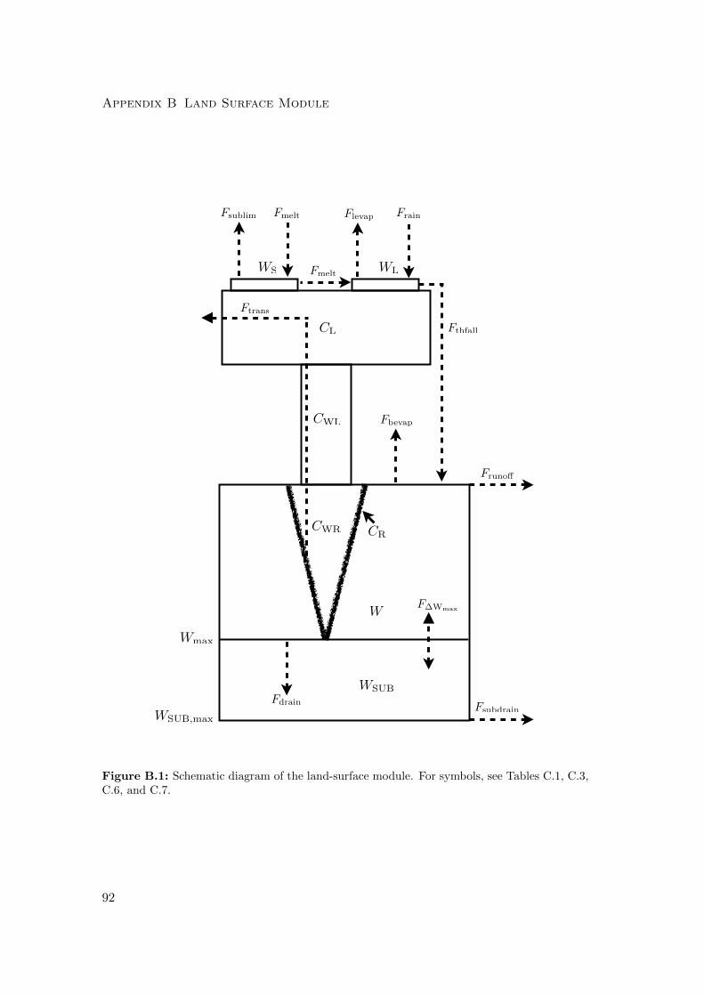
Appendix B Land Surface Module
WSUB,max
Wmax
CWL
CWR
CL
CR
W
WSUB
WS WLFmelt
Fthfall
FrainFmelt
Fruno↵
FsubdrainFdrain
F�Wmax
Fbevap
Fsublim Flevap
Ftrans
Figure B.1: Schematic diagram of the land-surface module. For symbols, see Tables C.1, C.3,C.6, and C.7.
92
B.1 Water storage and runoff generation
B.1 Water storage and runoff generation
The partitioning of precipitation between snow Psnow and rain Prain depends on near-
surface air temperature T following Wigmosta et al. (1994).
Psnow =
P T ≤ −1.1
P 3.3−T4.4 −1.1 < T < 3.3
0 T ≥ 3.3
(B.2)
Prain = P − Psnow
Rainfall is first intercepted in the canopy reservoir WL up to a maximum storage ca-
pacity WLmax which depends on LAI (see Eq. A.11). If a precipitation event causes
the water in the canopy reservoir to exceed its storage capacity, the excess water flows
from the canopy reservoir to the rooting zone as throughfall Fthfall.
Fthfall = max(0, WL + Prain −WLmax) (B.3)
Snowmelt Fmelt is computed according to a day-degree formula using a melt rate of
3.22 mm d−1 ◦C−1 (Hagemann and Dumenil 1997).
Fmelt =
0 T < 0
min (3.22 T, Psnow +WS) T ≥ 0(B.4)
Surface runoff Frunoff occurs when the throughfall or snowmelt fluxes cause the rooting
zone reservoir to exceed its maximum capacity WMAX (see Eq. A.11).
Frunoff =
Fthfall T ≤ 0
max (0, W + Fthfall + Fmelt −Wmax) T > 0(B.5)
When the air temperature drops below 0 ◦C, the soil is assumed to be frozen, inhibiting
infiltration, and the entire throughfall flux becomes surface runoff.
Drainage from the rooting zone Fdrain supplies water to the sub-rooting zone and
93
Appendix B Land Surface Module
depends on the soil wetness (fW = W/WMAX).
Fdrain =
0 fW ≤ 0.05
dmin fW; 0.05 < fW < 0.9
dmin fW + (dmax − dmin)(fW−0.91−0.9
)d; fW ≥ 0.9
(B.6)
When the rooting zone is between 5% and 90% of field capacity, it drains slowly (dmin =
0.24 mm d−1) with a linear dependence on soil wetness. When the rooting zone nears
saturation (fW ≥ 0.9), the drainage rate quickly increases with increasing wetness
towards its maximum drainage rate (dmax = 2.40 mm d−1). Drainage from the rooting
zone ceases when the soil wetness falls below 5%.
When the incoming drainage from the overlying rooting zone Fdrain causes the sub-
rooting zone to exceed its maximum capacity (WSUB,max), the excess flows out as sub-
rooting zone drainage Fsubdrain:
Fsubdrain = max (0, WSUB + Fdrain − (WSUB,max −Wmax)) (B.7)
where WSUB,max is maximum storage capacity of the entire soil column.
The flux term F∆Wmax accounts for changes in the depth of the rooting zone WMAX
(see Eq. A.11) due to the balance between carbon allocation to coarse root growth and
the loss of coarse root biomass via turnover.
F∆Wmax =
∆Wmax · WSUBWSUB,max−Wmax
∆Wmax < 0
∆Wmax · WWmax
∆Wmax > 0(B.8)
Coarse root growth (i.e. an increase in the depth of the rooting zone WMAX) leads
to a virtual flow of water from the sub-rooting zone to the rooting zone. Likewise, a
decrease in the depth of rooting zone due to coarse root turnover leads to a virtual flow
of water from the rooting zone to the sub-rooting zone.
94
B.2 Potential evapotranspiration
B.2 Potential evapotranspiration
The fractional snow area fSNOW depends on the amount of water in the snow cover
WS:
fSNOW = min(1,WS
WScrit) (B.9)
where WS,crit is the critical snow depth (water-equivalent). Following Robock (1980),
the albedo of snow as depends on air temperature T and the fractional forest cover
fFOR (see Eq. A.11).
as,min = 0.3 fFOR + 0.4 (1− fFOR)
as,max = 0.4 fFOR + 0.8 (1− fFOR)
as =
0 T ≥ 0
as,max − (as,max − as,min) T+1010 −10 < T < 0
1 T ≤ −10
(B.10)
The potential evapotranspiration fluxes for the snow-covered and snow-free fractions
are estimated using the Priestley-Taylor equation (Priestley and Taylor 1972) from the
net radiation fluxes described below, the slope of the saturation-vapor pressure curve
ε at air temperature T , the psychrometric constant Γ, the latent heat of vaporization
λ, and the Priestley-Taylor coefficient αp.
Ds = αpε(T )
ε(T ) + Γ
Rnet,s
λ
Dns = αpε(T )
ε(T ) + Γ
Rnet,ns
λ(B.11)
The net radiative energy available for evaporative processes Rnet is calculated separately
for the snow-covered and snow-free fractions from the downward shortwave Rsw↓ and
net longwave Rlw radiation fluxes, daylength h, and the albedo of the respective fraction
(as and ans).
Rnet,s = fSNOW 86400
(Rsw↓ (1− as) +
h
86400Rlw
)Rnet,ns = (1− fSNOW) 86400
(Rsw↓ (1− ans) +
h
86400Rlw
)(B.12)
95
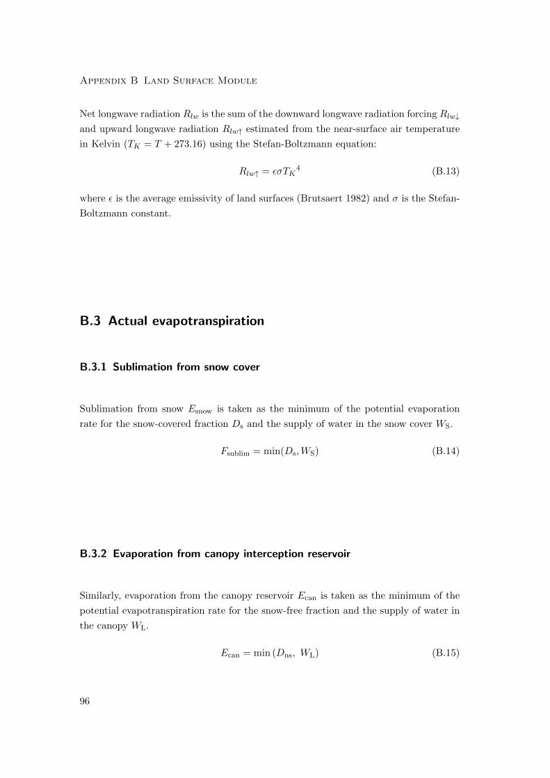
Appendix B Land Surface Module
Net longwave radiation Rlw is the sum of the downward longwave radiation forcing Rlw↓
and upward longwave radiation Rlw↑ estimated from the near-surface air temperature
in Kelvin (TK = T + 273.16) using the Stefan-Boltzmann equation:
Rlw↑ = εσTK4 (B.13)
where ε is the average emissivity of land surfaces (Brutsaert 1982) and σ is the Stefan-
Boltzmann constant.
B.3 Actual evapotranspiration
B.3.1 Sublimation from snow cover
Sublimation from snow Esnow is taken as the minimum of the potential evaporation
rate for the snow-covered fraction Ds and the supply of water in the snow cover WS.
Fsublim = min(Ds,WS) (B.14)
B.3.2 Evaporation from canopy interception reservoir
Similarly, evaporation from the canopy reservoir Ecan is taken as the minimum of the
potential evapotranspiration rate for the snow-free fraction and the supply of water in
the canopy WL.
Ecan = min (Dns, WL) (B.15)
96
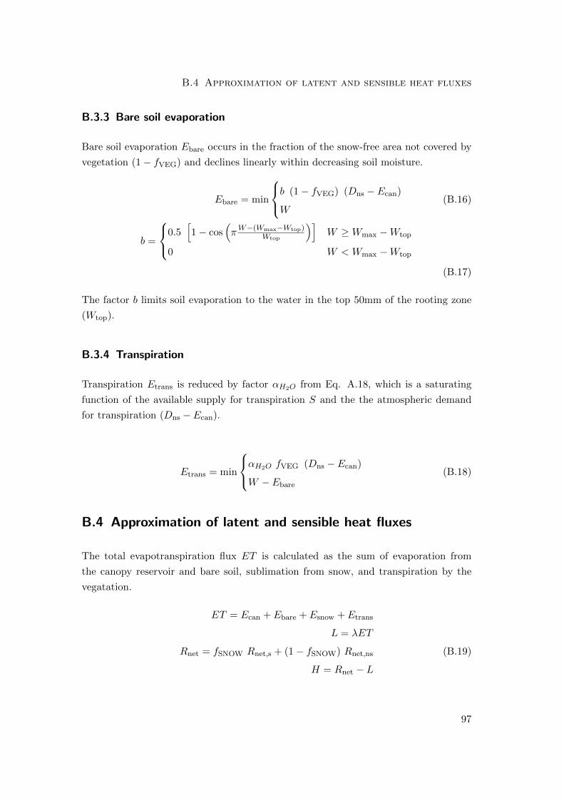
B.4 Approximation of latent and sensible heat fluxes
B.3.3 Bare soil evaporation
Bare soil evaporation Ebare occurs in the fraction of the snow-free area not covered by
vegetation (1− fVEG) and declines linearly within decreasing soil moisture.
Ebare = min
b (1− fVEG) (Dns − Ecan)
W(B.16)
b =
0.5[1− cos
(πW−(Wmax−Wtop)
Wtop
)]W ≥Wmax −Wtop
0 W < Wmax −Wtop
(B.17)
The factor b limits soil evaporation to the water in the top 50mm of the rooting zone
(Wtop).
B.3.4 Transpiration
Transpiration Etrans is reduced by factor αH2O from Eq. A.18, which is a saturating
function of the available supply for transpiration S and the the atmospheric demand
for transpiration (Dns − Ecan).
Etrans = min
αH2O fVEG (Dns − Ecan)
W − Ebare
(B.18)
B.4 Approximation of latent and sensible heat fluxes
The total evapotranspiration flux ET is calculated as the sum of evaporation from
the canopy reservoir and bare soil, sublimation from snow, and transpiration by the
vegatation.
ET = Ecan + Ebare + Esnow + Etrans
L = λET
Rnet = fSNOW Rnet,s + (1− fSNOW) Rnet,ns (B.19)
H = Rnet − L
97

Appendix B Land Surface Module
The latent heat flux L is estimated by multiplying the evapotranspiration flux by
the latent heat of vaporization for water λ. Total net radiation Rnet is computed as
the weighted combination of the net radiation over snow-covered and snow-free areas.
Sensible heat H is assumed to make up the difference between the net radiation and
latent heat fluxes.
98

Appendix C
Model parameters and variables
99
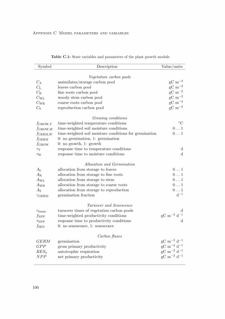
Appendix C Model parameters and variables
Table C.1: State variables and parameters of the plant growth module
Symbol Description Value/units
Vegetation carbon poolsCA assimilates/storage carbon pool gC m−2
CL leaves carbon pool gC m−2
CR fine roots carbon pool gC m−2
CWL woody stem carbon pool gC m−2
CWR coarse roots carbon pool gC m−2
CS reproduction carbon pool gC m−2
Growing conditionsfGROW,T time-weighted temperature conditions ◦CfGROW,W time-weighted soil moisture conditions 0 . . . 1fGERM,W time-weighted soil moisture conditions for germination 0 . . . 1fGERM 0: no germination, 1: germinationfGROW 0: no growth, 1: growthτT response time to temperature conditions dτW response time to moisture conditions d
Allocation and GerminationAL allocation from storage to leaves 0 . . . 1AR allocation from storage to fine roots 0 . . . 1AWL allocation from storage to stem 0 . . . 1AWR allocation from storage to coarse roots 0 . . . 1AS allocation from storage to reproduction 0 . . . 1γGERM germination fraction d−1
Turnover and Senescenceτtissue turnover times of vegetation carbon pools dfNPP time-weighted productivity conditions gC m−2 d−1
τNPP response time to productivity conditions dfSEN 0: no senescence, 1: senescence
Carbon fluxesGERM germination gC m−2 d−1
GPP gross primary productivity gC m−2 d−1
RESa autotrophic respiration gC m−2 d−1
NPP net primary productivity gC m−2 d−1
100
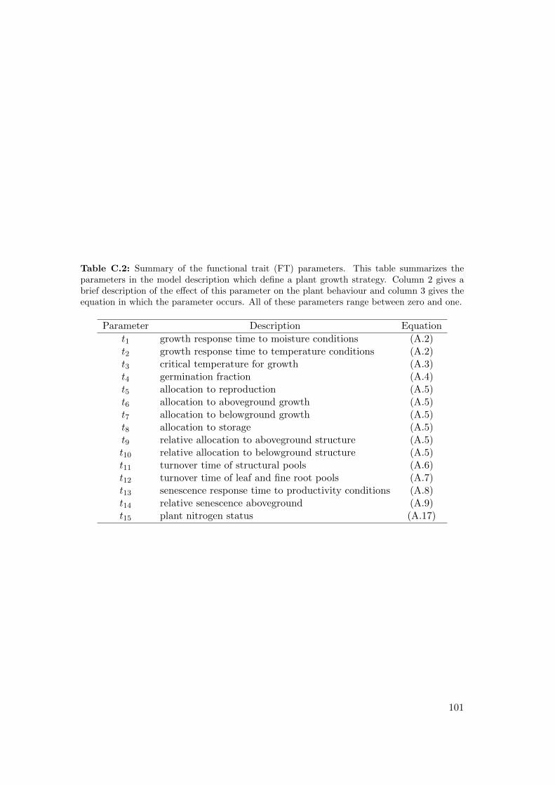
Table C.2: Summary of the functional trait (FT) parameters. This table summarizes theparameters in the model description which define a plant growth strategy. Column 2 gives abrief description of the effect of this parameter on the plant behaviour and column 3 gives theequation in which the parameter occurs. All of these parameters range between zero and one.
Parameter Description Equation
t1 growth response time to moisture conditions (A.2)t2 growth response time to temperature conditions (A.2)t3 critical temperature for growth (A.3)t4 germination fraction (A.4)t5 allocation to reproduction (A.5)t6 allocation to aboveground growth (A.5)t7 allocation to belowground growth (A.5)t8 allocation to storage (A.5)t9 relative allocation to aboveground structure (A.5)t10 relative allocation to belowground structure (A.5)t11 turnover time of structural pools (A.6)t12 turnover time of leaf and fine root pools (A.7)t13 senescence response time to productivity conditions (A.8)t14 relative senescence aboveground (A.9)t15 plant nitrogen status (A.17)
101
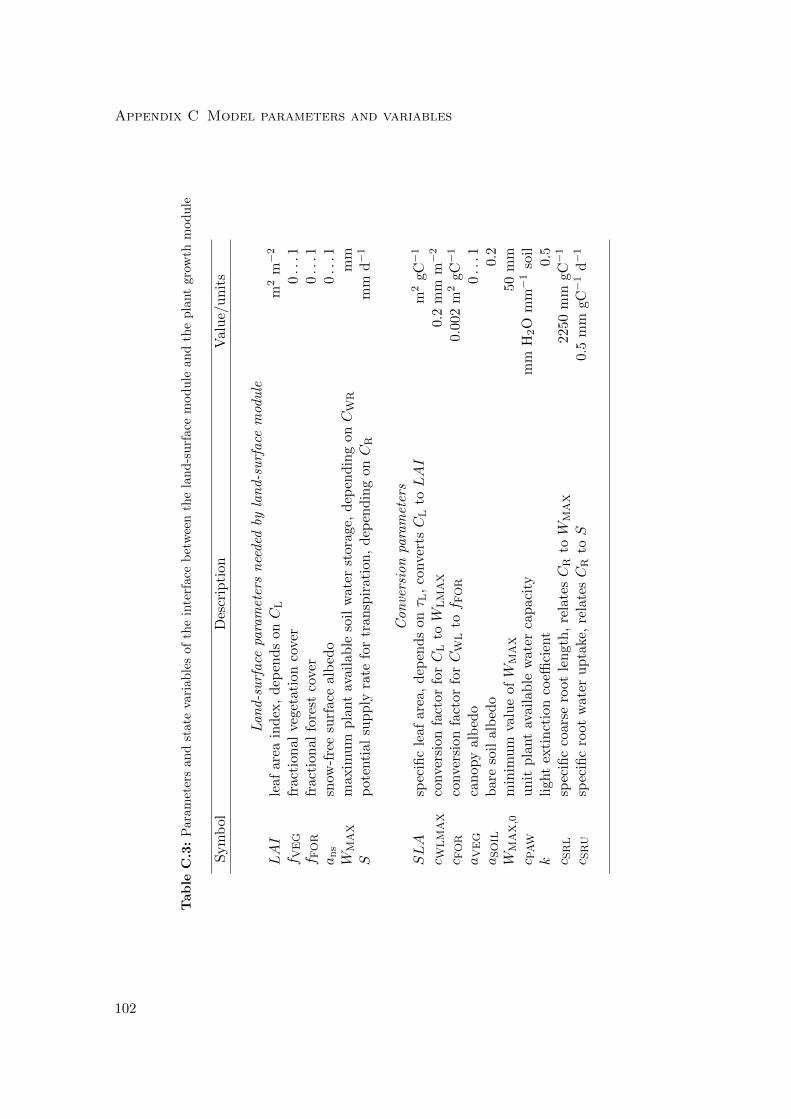
Appendix C Model parameters and variables
Table
C.3:
Par
amet
ers
and
stat
eva
riab
les
of
the
inte
rface
bet
wee
nth
ela
nd
-su
rface
mod
ule
an
dth
ep
lant
gro
wth
mod
ule
Sym
bol
Des
crip
tion
Val
ue/
un
its
Lan
d-s
urf
ace
para
met
ers
nee
ded
byla
nd-s
urf
ace
mod
ule
LAI
leaf
area
ind
ex,
dep
end
son
CL
m2
m−
2
f VE
Gfr
acti
onal
vege
tati
onco
ver
0...1
f FO
Rfr
acti
onal
fore
stco
ver
0...1
an
ssn
ow-f
ree
surf
ace
alb
edo
0...1
WM
AX
max
imu
mp
lant
avai
lab
leso
ilw
ater
stor
age,
dep
end
ing
onC
WR
mm
Sp
oten
tial
sup
ply
rate
for
tran
spir
atio
n,
dep
end
ing
onC
Rm
md−
1
Con
vers
ion
para
met
ers
SLA
spec
ific
leaf
area
,d
epen
ds
onτ L
,co
nve
rtsC
LtoLAI
m2
gC−
1
c WL
MA
Xco
nve
rsio
nfa
ctor
forC
LtoW
LM
AX
0.2
mm
m−
2
c FO
Rco
nve
rsio
nfa
ctor
forC
WL
tof F
OR
0.00
2m
2gC−
1
aV
EG
can
opy
alb
edo
0...1
aS
OIL
bar
eso
ilal
bed
o0.2
WM
AX,0
min
imu
mva
lue
ofW
MA
X50
mm
c PA
Wu
nit
pla
nt
avai
lab
lew
ater
cap
acit
ym
mH
2O
mm−
1so
ilk
ligh
tex
tin
ctio
nco
effici
ent
0.5
c SR
Lsp
ecifi
cco
arse
root
len
gth
,re
late
sC
RtoW
MA
X22
50m
mgC−
1
c SR
Usp
ecifi
cro
otw
ater
up
take
,re
late
sC
RtoS
0.5
mm
gC−
1d−
1
102
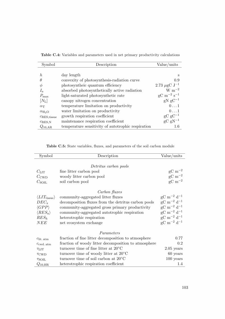
Table C.4: Variables and parameters used in net primary productivity calculations
Symbol Description Value/units
h day length sθ convexity of photosynthesis-radiation curve 0.9φ photosyntheic quantum efficiency 2.73 µgC J−1
Ia absorbed photosynthetically active radiation W m−2
Pmax light-saturated photosynthetic rate gC m−2 s−1
[NL] canopy nitrogen concentration gN gC−1
αT temperature limitation on productivity 0 . . . 1αH2O water limitation on productivity 0 . . . 1cRES,tissue growth respiration coefficient gC gC−1
cRES,N maintenance respiration coefficient gC gN−1
Q10,AR temperature sensitivity of autotrophic respiration 1.6
Table C.5: State variables, fluxes, and parameters of the soil carbon module
Symbol Description Value/units
Detritus carbon poolsCLIT fine litter carbon pool gC m−2
CCWD woody litter carbon pool gC m−2
CSOIL soil carbon pool gC m−2
Carbon fluxes〈LITtissue〉 community-aggregated litter fluxes gC m−2 d−1
DECx decomposition fluxes from the detritus carbon pools gC m−2 d−1
〈GPP 〉 community-aggregated gross primary productivity gC m−2 d−1
〈RESa〉 community-aggregated autotrophic respiration gC m−2 d−1
RESh heterotrophic respiration gC m−2 d−1
NEE net ecosystem exchange gC m−2 d−1
Parametersclit.atm fraction of fine litter decomposition to atmosphere 0.77ccwd.atm fraction of woody litter decomposition to atmosphere 0.2τLIT turnover time of fine litter at 20◦C 2.05 yearsτCWD turnover time of woody litter at 20◦C 60 yearsτSOIL turnover time of soil carbon at 20◦C 100 yearsQ10,HR heterotrophic respiration coefficient 1.4
103
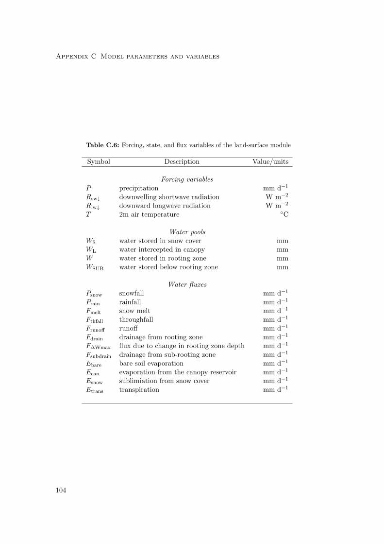
Appendix C Model parameters and variables
Table C.6: Forcing, state, and flux variables of the land-surface module
Symbol Description Value/units
Forcing variablesP precipitation mm d−1
Rsw↓ downwelling shortwave radiation W m−2
Rlw↓ downward longwave radiation W m−2
T 2m air temperature ◦C
Water poolsWS water stored in snow cover mmWL water intercepted in canopy mmW water stored in rooting zone mmWSUB water stored below rooting zone mm
Water fluxesPsnow snowfall mm d−1
Prain rainfall mm d−1
Fmelt snow melt mm d−1
Fthfall throughfall mm d−1
Frunoff runoff mm d−1
Fdrain drainage from rooting zone mm d−1
F∆Wmax flux due to change in rooting zone depth mm d−1
Fsubdrain drainage from sub-rooting zone mm d−1
Ebare bare soil evaporation mm d−1
Ecan evaporation from the canopy reservoir mm d−1
Esnow sublimiation from snow cover mm d−1
Etrans transpiration mm d−1
104
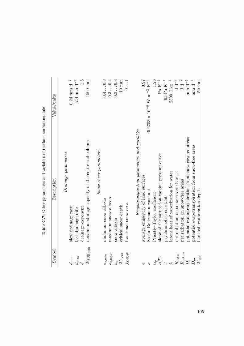
Table
C.7:
Oth
erp
ara
met
ers
an
dva
riab
les
of
the
lan
d-s
urf
ace
mod
ule
Sym
bol
Des
crip
tion
Val
ue/
un
its
Dra
inage
para
met
ers
dm
insl
owd
rain
age
rate
0.24
mm
d−
1
dm
ax
fast
dra
inag
era
te2.
4m
md−
1
dd
rain
age
exp
onen
t1.
5W
SU
Bm
ax
max
imu
mst
orag
eca
pac
ity
ofth
een
tire
soil
colu
mn
1500
mm
Sn
ow
cove
rpa
ram
eter
sa
s,m
inm
inim
um
snow
alb
edo
0.4...0.8
as,
max
max
imu
msn
owal
bed
o0.
3...0.4
as
snow
alb
edo
0.3...0.8
WS,c
rit
crit
ical
snow
dep
th10
mm
f SN
OW
frac
tion
alsn
owar
ea0...1
Eva
potr
an
spir
ati
on
para
met
ers
an
dva
riabl
esε
aver
age
emis
sivit
yof
lan
dsu
rfac
es0.
97σ
Ste
fan
-Bol
tzm
ann
con
stan
t5.6
703×
10−
8W
m−
2K−
4
αp
Pri
estl
y-T
aylo
rco
effici
ent
1.26
ε(T
)sl
ope
ofth
esa
tura
tion
-vap
our
pre
ssu
recu
rve
Pa
K−
1
Γp
sych
rom
etri
cco
nst
ant
65P
aK−
1
λla
tent
hea
tof
vap
oriz
atio
nfo
rw
ater
2500
Jkg−
1
Rn
et,s
net
rad
iati
onon
snow
-cov
ered
area
sJ
d−
2
Rn
et,n
sn
etra
dia
tion
onsn
ow-f
ree
area
sJ
d−
2
Ds
pot
enti
alev
apot
ran
spir
atio
nfr
omsn
ow-c
over
edar
eas
mm
d−
1
Dn
sp
oten
tial
evap
otra
nsp
irat
ion
from
snow
-fre
ear
eas
mm
d−
1
Wto
pb
are
soil
evap
orat
ion
dep
th50
mm
105

Bibliography
Ackerly, D. and Cornwell, W. K. (2007). A trait-based approach to community assem-
bly: partitioning of species trait values into within- and among-community compo-
nents. Ecology Letters, 10(2):135–145.
Ainsworth, E. A. and Long, S. P. (2004). What have we learned from 15 years of free-air
CO2 enrichment (FACE)? A meta-analytic review of the responses of photosynthe-
sis, canopy properties and plant production to rising CO2. The New Phytologist,
165(2):351–372.
Allan, E., Weisser, W., Weigelt, A., Roscher, C., Fischer, M., and Hillebrand, H. (2011).
More diverse plant communities have higher functioning over time due to turnover in
complementary dominant species. Proceedings of the National Academy of Sciences
of the United States of America, 108(41):17034–17039.
Alton, P. B. (2011). How useful are plant functional types in global simulations of the
carbon, water, and energy cycles? Journal of Geophysical Research, 116(G01030).
Alvarado, V. and Bradford, K. (2002). A hydrothermal time model explains the cardinal
temperatures for seed germination. Plant, Cell & Environment, 25(8):1061–1069.
Arora, V. and Boer, G. (2006). Simulating competition and coexistence between plant
functional types in a dynamic vegetation model. Earth Interactions, 10(10):1–30.
Asner, G. P. and Alencar, A. (2010). Drought impacts on the Amazon forest: the
remote sensing perspective. The New Phytologist, 187(3):569–578.
Axelsson, E. and Axelsson, B. (1986). Changes in carbon allocation patterns in spruce
and pine trees following irrigation and fertilization. Tree Physiology, 2(1 2 3):189–
204.
Baas-Becking, L. (1934). Geobiologie of inleiding tot de milieukunde. van Stockum and
Zoon, The Hague, Netherlands.
107
Bibliography
Baker, D., Law, R., Gurney, K., Rayner, P., Peylin, P., Denning, A., Bousquet, P.,
Bruhwiler, L., Chen, Y., Ciais, P., Fung, I., Heimann, M., John, J., Maki, T.,
Maksyutov, S., Masarie, K., Prather, M., Pak, B., Taguchi, S., and Zhu, Z. (2006).
TransCom 3 inversion intercomparison: Impact of transport model errors on the in-
terannual variability of regional CO2 fluxes, 1988-2003. Global Biogeochemical Cycles,
20(GB1002).
Balvanera, P., Pfisterer, A. B., Buchmann, N., He, J.-S., Nakashizuka, T., Raffaelli, D.,
and Schmid, B. (2006). Quantifying the evidence for biodiversity effects on ecosystem
functioning and services. Ecology Letters, 9(10):1146–1156.
Beer, C., Reichstein, M., Tomelleri, E., Ciais, P., Jung, M., Carvalhais, N., Rodenbeck,
C., Arain, M. A., Baldocchi, D. D., Bonan, G., Bondeau, A., Cescatti, A., Lasslop,
G., Lindroth, A., Lomas, M., Luyssaert, S., Margolis, H., Oleson, K. W., Roupsard,
O., Veenendaal, E., Viovy, N., Williams, C., Woodward, F. I., and Papale, D. (2010).
Terrestrial Gross Carbon Dioxide Uptake: Global Distribution and Covariation with
Climate. Science, 329(5993):834–838.
Bloom, A. J., Chapin, F. S. I., and Mooney, H. (1985). Resource Limitation in Plants-
An Economic Analogy. Annual Review of Ecology and Systematics, 16(1):363–392.
Bohn, K., Dyke, J. G., Pavlick, R., Reineking, B., Reu, B., and Kleidon, A. (2011). The
relative importance of seed competition, resource competition and perturbations on
community structure. Biogeosciences, 8(5):1107–1120.
Bonan, G. and Levis, S. (2006). Evaluating aspects of the community land and atmo-
sphere models (CLM3 and CAM3) using a dynamic global vegetation model. Journal
of Climate, 19(11):2290–2301.
Bonan, G., Levis, S., Kergoat, L., and Oleson, K. W. (2002). Landscapes as patches
of plant functional types: An integrating concept for climate and ecosystem models.
Global Biogeochemical Cycles, 16(2):1–18.
Box, E. (1996). Plant functional types and climate at the global scale. Journal of
Vegetation Science, 7(3):309–320.
Bruggeman, J. and Kooijman, S. A. L. M. (2007). A biodiversity-inspired approach to
aquatic ecosystem modeling. Limnology and Oceanography, 52(4):1533–1544.
Brutsaert, W. (1982). Evaporation into the atmosphere. theory, history, and applica-
tions. Kluwer Academic Publishers, Dordrecht, The Netherlands.
108
Bibliography
Cannell, M. G. R. (1982). World forest biomass and primary production data. Academic
Press, London, UK.
Cannell, M. G. R. and Thornley, J. H. M. (1998). Temperature and CO2 Responses of
Leaf and Canopy Photosynthesis: a Clarification using the Non-rectangular Hyper-
bola Model of Photosynthesis. Annals of Botany, 82(6):883–892.
Cardinale, B. J., Matulich, K. L., Hooper, D. U., Byrnes, J. E., Duffy, E., Gamfeldt,
L., Balvanera, P., O’Connor, M. I., and Gonzalez, A. (2011). The functional role of
producer diversity in ecosystems. American Journal of Botany, 98(3):572–592.
Cavender-Bares, J., Kozak, K. H., Fine, P. V. A., and Kembel, S. W. (2009). The
merging of community ecology and phylogenetic biology. Ecology Letters, 12(7):693–
715.
Chapin, F. S. I., BretHarte, M., Hobbie, S., and Zhong, H. (1996). Plant functional
types as predictors of transient responses of arctic vegetation to global change. Jour-
nal of Vegetation Science, 7(3):347–358.
Chave, J., Coomes, D., Jansen, S., Lewis, S. L., Swenson, N. G., and Zanne, A. E.
(2009). Towards a worldwide wood economics spectrum. Ecology Letters, 12(4):351–
366.
Cohen, D. (1968). A General Model of Optimal Reproduction in a Randomly Varying
Environment. Journal of Ecology, 56(1):219–228.
Cornwell, W. K. and Ackerly, D. (2009). Community assembly and shifts in plant
trait distributions across an environmental gradient in coastal California. Ecological
Monographs, 79(1):109–126.
Cox, P. (2001). Description of the TRIFFID dynamic global vegetation model. Hadley
Centre, Bracknell, UK.
Cox, P., Betts, R. A., Jones, C. D., Spall, S. A., and Totterdell, I. J. (2000). Acceleration
of global warming due to carbon-cycle feedbacks in a coupled climate model. Nature,
408(6809):184–187.
Cramer, W., Bondeau, A., Woodward, F. I., Prentice, I. C., Betts, R. A., Brovkin,
V., Cox, P., Fisher, V., Foley, J. A., Friend, A. D., Kucharik, C., Lomas, M. R.,
Ramankutty, N., Sitch, S., Smith, B., White, A., and Young-Molling, C. (2001).
Global response of terrestrial ecosystem structure and function to CO 2and climate
109

Bibliography
change: results from six dynamic global vegetation models. Global Change Biology,
7(4):357–373.
Darwin, C. (1987). Charles Darwin’s Natural Selection: Being the Second Part of his
Big Species Book Written from 1856 to 1858. Cambridge University Press.
Denman, K., Brasseur, G., Chidthaisong, A., Ciais, P., Cox, P., Dickinson, R., Hauglus-
taine, D., Heinze, C., Holland, E., Jacob, D., Lohnmann, U., Ramachandran, S.,
da Silva Dias, P., Wofsy, S. C., and Zhang, X. (2007). Couplings Between Changes
in the Climate System and Biogeochemistry. In Solomon, S., Qin, D., Manning, M.,
Chen, Z., Marquis, M., Averyt, K., Tignor, M., and Miller, H. L., editors, Climate
Change 2007: The Physical Science Basis. Contribution of Working Group I to the
Fourth Assessment Report of the Intergovernmental Panel on Climate Change. Cli-
mate Change 2007: The Physical Science Basis. Contribution of Working Group I to
the Fourth Assessment Report of the Intergovernmental Panel on Climate Change,
Cambridge, United Kingdom.
Dıaz, S. and Cabido, M. (2001). Vive la difference: plant functional diversity matters
to ecosystem processes. Trends in Ecology & Evolution, 16(11):646–655.
Dıaz, S., Fargione, J., Chapin, F. S. I., and Tilman, D. (2006). Biodiversity loss
threatens human well-being. Plos Biology, 4(8):1300–1305.
Dıaz, S., Lavorel, S., de Bello, F., Quetier, F., Grigulis, K., and Robson, T. M. (2007).
Incorporating plant functional diversity effects in ecosystem service assessments.
Proceedings of the National Academy of Sciences of the United States of America,
104(52):20684–20689.
Doak, D. F., Bigger, D., Harding, E. K., Marvier, M. A., O’Malley, R. E., and Thom-
son, D. (1998). The Statistical Inevitability of StabilityDiversity Relationships in
Community Ecology. http://dx.doi.org/10.1086/286117.
Doney, S., Lindsay, K., Fung, I., and John, J. (2006). Natural Variability in a Stable,
1000-Yr Global Coupled Climate–Carbon Cycle Simulation. Journal of Climate,
19(13):3033–3054.
Drewry, D. T., Kumar, P., Long, S., Bernacchi, C., Liang, X., and Sivapalan, M. (2010).
Ecohydrological responses of dense canopies to environmental variability: 1. Inter-
play between vertical structure and photosynthetic pathway. Journal of Geophysical
Research-Biogeosciences, 115(G04022).
110
Bibliography
Dunne, K. and Willmott, C. (1996). Global Distribution of Plant Extractable Water
Capacity of Soil. International Journal of Climatology, 16(8):841–859.
Dutkiewicz, S., Follows, M. J., and Bragg, J. G. (2009). Modeling the coupling of ocean
ecology and biogeochemistry. Global Biogeochemical Cycles, 23(GB4017).
Elmqvist, T., Folke, C., Nystrom, M., Peterson, G., Bengtsson, J., Walker, B., and
Norberg, J. (2003). Response diversity, ecosystem change, and resilience. Frontiers
in Ecology and the Environment, 1(9):488–494.
Elser, J. J., Bracken, M. E. S., Cleland, E. E., Gruner, D. S., Harpole, W. S., Hillebrand,
H., Ngai, J. T., Seabloom, E. W., Shurin, J. B., and Smith, J. E. (2007). Global
analysis of nitrogen and phosphorus limitation of primary producers in freshwater,
marine and terrestrial ecosystems. Ecology Letters, 10(12):1135–1142.
Ezoe, H. (1998). Optimal dispersal range and seed size in a stable environment . Journal
of Theoretical Biology, 190(3):287–293.
Falge, E., Baldocchi, D. D., Tenhunen, J., Aubinet, M., Bakwin, P., Berbigier, P.,
Bernhofer, C., Burba, G., Clement, R., Davis, K. J., Elbers, J. A., Goldstein, A. H.,
Grelle, A., Granier, A., Guomundsson, J., Hollinger, D., Kowalski, A. S., Katul,
G., Law, B. E., Malhi, Y., Meyers, T., Monson, R. K., Munger, J. W., Oechel, W.,
Paw U, K. T., Pilegaard, K., Rannik, U., Rebmann, C., Suyker, A., Valentini, R.,
Wilson, K., and Wofsy, S. (2002). Seasonality of ecosystem respiration and gross
primary production as derived from FLUXNET measurements. Agricultural and
Forest Meteorology, 113(1-4):53–74.
Falster, D. S., Brannstrom, A., Dieckmann, U., and Westoby, M. (2010). Influence of
four major plant traits on average height, leaf-area cover, net primary productivity,
and biomass density in single-species forests: a theoretical investigation. Journal of
Ecology, 99(1):148–164.
Figueira, A. M. e. S., Miller, S. D., de Sousa, C. A. D., Menton, M. C., Maia, A. R.,
da Rocha, H. R., and Goulden, M. L. (2008). Effects of selective logging on tropical
forest tree growth. Journal of Geophysical Research-Biogeosciences, 113(G00B05).
Fisher, J. B., Sitch, S., Malhi, Y., FISHER, R. A., Huntingford, C., and Tan, S. Y.
(2010a). Carbon cost of plant nitrogen acquisition: A mechanistic, globally applicable
model of plant nitrogen uptake, retranslocation, and fixation. Global Biogeochemical
Cycles, 24(GB1014).
111
Bibliography
Fisher, R., McDowell, N., Purves, D., Moorcroft, P., Sitch, S., Cox, P., Huntingford,
C., Meir, P., and Woodward, F. I. (2010b). Assessing uncertainties in a second-
generation dynamic vegetation model caused by ecological scale limitations. The
New Phytologist, 187(3):666–681.
Fisher, R., Williams, M., Lola da Costa, A., Malhi, Y., Lola da Costa, R. F., Almeida,
S., and Meir, P. (2007). The response of an Eastern Amazonian rain forest to drought
stress: results and modelling analyses from a throughfall exclusion experiment. Global
Change Biology, 13(11):2361–2378.
Flombaum, P. and Sala, O. E. (2008). From the Cover: Higher effect of plant species
diversity on productivity in natural than artificial ecosystems. Proceedings of the
National Academy of Sciences of the United States of America, 105(16):6087–6090.
Foley, J. A., Levis, S., Costa, M., Cramer, W., and Pollard, D. (2000). Incorporat-
ing dynamic vegetation cover within global climate models. Ecological Applications,
10(6):1620–1632.
Foley, J. A., Prentice, I. C., Ramankutty, N., Levis, S., Pollard, D., Sitch, S., and
Haxeltine, A. (1996). An integrated biosphere model of land surface processes, ter-
restrial carbon balance, and vegetation dynamics. Global Biogeochemical Cycles,
10(4):603–628.
Follows, M. J. and Dutkiewicz, S. (2011). Modeling Diverse Communities of Marine
Microbes. Annual Review of Marine Science, 3:427–451.
Follows, M. J., Dutkiewicz, S., Grant, S., and Chisholm, S. W. (2007). Emergent
Biogeography of Microbial Communities in a Model Ocean. Science, 315(5820):1843–
1846.
Franklin, O. (2007). Optimal nitrogen allocation controls tree responses to elevated
CO2. The New Phytologist, 174(4):811–822.
Freschet, G. T., Dias, A. T. C., Ackerly, D., Aerts, R., Van Bodegom, P. M., Cornwell,
W. K., Dong, M., Kurokawa, H., Liu, G., Onipchenko, V. G., Ordonez, J. C., Peltzer,
D. A., Richardson, S. J., Shidakov, I. I., Soudzilovskaia, N. A., Tao, J., and Cor-
nelissen, J. H. C. (2011). Global to community scale differences in the prevalence of
convergent over divergent leaf trait distributions in plant assemblages. Global Ecology
and Biogeography, 20(5):755–765.
112
Bibliography
Friedlingstein, P., Cox, P., Betts, R. A., Bopp, L., von Bloh, W., Brovkin, V., Cadule,
P., Doney, S., Eby, M., Fung, I., Bala, G., John, J., Jones, C., Joos, F., Kato, T.,
Kawamiya, M., Knorr, W., Lindsay, K., Matthews, H. D., Raddatz, T., Rayner,
P., Reick, C., Roeckner, E., Schnitzler, K. G., Schnur, R., Strassmann, K., Weaver,
A. J., Yoshikawa, C., and Zeng, N. (2006). Climate–Carbon Cycle Feedback Analysis:
Results from the C 4MIP Model Intercomparison. Journal of Climate, 19(14):3337–
3353.
Friedlingstein, P., Joel, G., Field, C. B., and Fung, I. Y. (1999). Toward an allocation
scheme for global terrestrial carbon models. Global Change Biology, 5(7):755–770.
Friend, A., Stevens, A., Knox, R., and Cannell, M. G. R. (1997). A process-based, ter-
restrial biosphere model of ecosystem dynamics (Hybrid v3.0). Ecological Modelling,
95:249–287.
Fung, I. Y., Doney, S., Lindsay, K., and John, J. (2005). Evolution of carbon sinks in
a changing climate. Proceedings of the National Academy of Sciences of the United
States of America, 102(32):11201–11206.
Garnier, E., Cortez, J., Billes, G., Navas, M., Roumet, C., Debussche, M., Laurent,
G., Blanchard, A., Aubry, D., Bellmann, A., Neill, C., and Toussaint, J. (2004).
Plant functional markers capture ecosystem properties during secondary succession.
Ecology, 85(9):2630–2637.
Grime, J. (1998). Benefits of plant diversity to ecosystems: immediate, filter and
founder effects. Journal of Ecology, 86(6):902–910.
Groenendijk, M., Dolman, A. J., van der Molen, M. K., Leuning, R., Arneth, A.,
Delpierre, N., Gash, J. H. C., Lindroth, A., Richardson, A. D., and Verbeeck, H.
(2011). Assessing parameter variability in a photosynthesis model within and between
plant functional types using global Fluxnet eddy covariance data. Agricultural and
Forest Meteorology, 151(1):22–38.
Gu, L., Baldocchi, D., Wofsy, S., Munger, J., Michalsky, J., Urbanski, S., and Boden, T.
(2003). Response of a deciduous forest to the Mount Pinatubo eruption: Enhanced
photosynthesis. Science, 299(5615):2035–2038.
Gurney, K., Law, R., Denning, A., Rayner, P., Pak, B., Baker, D., Bousquet, P., Bruh-
wiler, L., Chen, Y., Ciais, P., Fung, I., Heimann, M., John, J., Maki, T., Maksyutov,
113
Bibliography
S., Peylin, P., Prather, M., and Taguchi, S. (2004). Transcom 3 inversion intercom-
parison: Model mean results for the estimation of seasonal carbon sources and sinks.
Global Biogeochemical Cycles, 18(GB1010).
Haddeland, I., Clark, D. B., Franssen, W., Ludwig, F., Voß, F., Arnell, N. W., Bertrand,
N., Best, M., Folwell, S., Gerten, D., Gomes, S., Gosling, S. N., Hagemann, S.,
Hanasaki, N., Harding, R., Heinke, J., Kabat, P., Koirala, S., Oki, T., Polcher, J.,
Stacke, T., Viterbo, P., Weedon, G. P., and Yeh, P. (2011). Multimodel Estimate of
the Global Terrestrial Water Balance: Setup and First Results. Journal of Hydrom-
eteorology, 12(5):869–884.
Hagemann, S. and Dumenil, L. (1997). A parametrization of the lateral waterflow for
the global scale. Climate Dynamics, 14(1):17–31.
Hall, C., Stanford, J., and Hauer, F. (1992). The Distribution and Abundance of Organ-
isms as a Consequence of Energy Balances Along Multiple Environmental Gradients.
Oikos, 65(3):377–390.
Harrison, S. P., Prentice, I. C., Barboni, D., Kohfeld, K. E., Ni, J., and Sutra, J.-P.
(2010). Ecophysiological and bioclimatic foundations for a global plant functional
classification. Journal of Vegetation Science, 21(2):300–317.
Hartmann, D. L. (1994). Global Physical Climatology. International Geophysics Series.
Academic Press, San Francisco, 1 edition.
Hector, A., Schmid, B., Beierkuhnlein, C., Caldeira, M., Diemer, M., Dimitrakopou-
los, P., Finn, J., Freitas, H., Giller, P., and Good, J. (1999). Plant diversity and
productivity experiments in European grasslands. Science, 286(5442):1123–1127.
Heinsch, F., Zhao, M., Running, S. W., Kimball, J. S., Nemani, R. R., Davis, K. J.,
Bolstad, P. V., Cook, B. D., Desai, A. R., Ricciuto, D. M., LAW, B. E., Oechel, W. C.,
Kwon, H., Luo, H., Wofsy, S. C., Dunn, A. L., Munger, J. W., Baldocchi, D. D., Xu,
L., Hollinger, D. Y., Richardson, A. D., Stoy, P. C., Siqueira, M. B. S., Monson,
R. K., Burns, S. P., and Flanagan, L. B. (2006). Evaluation of remote sensing
based terrestrial productivity from MODIS using regional tower eddy flux network
observations. Geoscience and Remote Sensing, IEEE Transactions on, 44(7):1908–
1925.
Hickler, T., Prentice, I. C., Smith, B., Sykes, M. T., and Zaehle, S. (2006). Implement-
ing plant hydraulic architecture within the LPJ Dynamic Global Vegetation Model.
Global Ecology and Biogeography, 15(6):567–577.
114
Bibliography
Hickler, T., Smith, B., Prentice, I. C., Mjofors, K., Miller, P., Arneth, A., and Sykes,
M. T. (2008). CO2 fertilization in temperate FACE experiments not representative
of boreal and tropical forests. Global Change Biology, 14(7):1531–1542.
Hollinger, D. Y., Ollinger, S. V., Richardson, A. D., Meyers, T. P., Dail, D. B., Martin,
M. E., Scott, N. A., Arkebauer, T. J., Baldocchi, D. D., Clark, K. L., Curtis, P. S.,
Davis, K. J., Desai, A. R., Dragoni, D., Goulden, M. L., Gu, L., Katul, G. G.,
Pallardy, S. G., Paw U, K. T., Schmid, H. P., Stoy, P. C., Sukyer, A. E., and
Verma, S. B. (2010). Albedo estimates for land surface models and support for
a new paradigm based on foliage nitrogen concentration. Global Change Biology,
16(2):696–710.
Hooper, D., Chapin, F. S. I., Ewel, J., Hector, A., Inchausti, P., Lavorel, S., Lawton, J.,
Lodge, D., Loreau, M., Naeem, S., Schmid, B., Setala, H., Symstad, A., Vandermeer,
J., and Wardle, D. (2005). Effects of biodiversity on ecosystem functioning: A
consensus of current knowledge. Ecological Monographs, 75(1):3–35.
Houghton, R. A., Hall, F., and Goetz, S. J. (2009). Importance of biomass in the global
carbon cycle. Journal of Geophysical Research-Biogeosciences, 114(G00E03).
Hubbell, S. P. (1979). Tree dispersion, abundance, and diversity in a tropical dry forest.
Science, 203(4387):1299–1309.
Hubbell, S. P. (1997). A unified theory of biogeography and relative species abundance
and its application to tropical rain forests and coral reefs. Coral Reefs, 16(5):S9–S21.
Ito, A. (2011). A historical meta-analysis of global terrestrial net primary productivity:
are estimates converging? Global Change Biology, 17(10):3161–3175.
Ives, A. R. and Carpenter, S. R. (2007). Stability and Diversity of Ecosystems. Science,
317(5834):58–62.
Jackson, S. and Williams, J. (2004). Modern analogs in Quaternary paleoecology:
Here today, gone yesterday, gone tomorrow? Annual Review of Earth and Planetary
Sciences, 32:495–537.
Johnson, I. R. and Thornley, J. H. M. (1984). A model of instantaneous and daily
canopy photosynthesis. Journal of Theoretical Biology, 107(4):531–545.
Jung, M., Reichstein, M., and Bondeau, A. (2009). Towards global empirical upscaling
of FLUXNET eddy covariance observations: validation of a model tree ensemble
approach using a biosphere model. Biogeosciences, 6(10):2001–2013.
115
Bibliography
Jung, M., Reichstein, M., Ciais, P., Seneviratne, S. I., Sheffield, J., Goulden, M. L.,
Bonan, G., Cescatti, A., Chen, J., de Jeu, R., Dolman, A. J., Eugster, W., Gerten,
D., Gianelle, D., Gobron, N., Heinke, J., Kimball, J., Law, B. E., Montagnani, L.,
Mu, Q., Mueller, B., Oleson, K. W., Papale, D., Richardson, A. D., Roupsard, O.,
Running, S., Tomelleri, E., Viovy, N., Weber, U., Williams, C., Wood, E. F., Zaehle,
S., and Zhang, K. (2010). Recent decline in the global land evapotranspiration trend
due to limited moisture supply. Nature, 467(7318):951–954.
Kaduk, J. and Heimann, M. (1996). Assessing the climate sensitivity of the global
terrestrial carbon cycle model SILVAN. Physics and Chemistry of The Earth, 21:529–
535.
Kattge, J., Dıaz, S., Lavorel, S., Prentice, I. C., Leadley, P., Bonisch, G., Garnier, E.,
Westoby, M., Reich, P., Wright, I. J., Cornelissen, J. H. C., Violle, C., Harrison,
S., van Bodegom, P., Reichstein, M., Enquist, B., Soudzilovskaia, N., Ackerly, D.,
Anand, M., Atkin, O., Bahn, M., Baker, T., Baldocchi, D. D., Bekker, R., Blanco,
C., Blonder, B., Bond, W., Bradstock, R., Bunker, D., Casanoves, F., Cavender-
Bares, J., Chambers, J. Q., Chapin, F. S. I., Chave, J., Coomes, D., Cornwell, W.,
Craine, J., Dobrin, B., Duarte, L., Durka, W., Elser, J., Esser, G., Estiarte, M.,
Fagan, W., Fang, J., Fernandez-Mendez, F., Fidelis, A., Finegan, B., Flores, O.,
Ford, H., Frank, D., Freschet, G., Fyllas, N., Gallagher, R., Green, W., Gutierrez,
A., Hickler, T., Higgins, S. L., Hodgson, J., Jalili, A., Jansen, S., Joly, C., Kerkhoff,
A., Kirkup, D., Kitajima, K., Kleyer, M., Klotz, S., Knops, J., Kramer, K., Kuhn,
I., Kurokawa, H., Laughlin, D., Lee, T., Leishman, M., Lens, F., Lenz, T., Lewis, S.,
Lloyd, J., Llusia, J., Louault, F., Ma, S., Mahecha, M., Manning, P., Massad, T.,
Medlyn, B., Messier, J., Moles, A., Muller, S., Nadrowski, K., Naeem, S., Niinemets,
U., Nollert, S., Nuske, A., Ogaya, R., Oleksyn, J., Onipchenko, V., Onoda, Y.,
Ordonez, J., Overbeck, G., Ozinga, W., Patino, S., Paula, S., Pausas, J., Penuelas,
J., Phillips, O., Pillar, V., Poorter, H., Poorter, L., Poschlod, P., Prinzing, A.,
Proulx, R., Rammig, A., Reinsch, S., Reu, B., Sack, L., Salgado-Negret, B., Sardans,
J., Shiodera, S., Shipley, B., Siefert, A., Sosinski, E., Soussana, j.-F., Swaine, E.,
Swenson, N., Thompson, K., Thornton, P., Waldram, M., Weiher, E., White, M.,
White, S., Wright, J., Yguel, B., Zaehle, S., Zanne, A., and Wirth, C. (2011). TRY
– a global database of plant traits. Global Change Biology, 17(9):2905–2935.
Kattge, J., Knorr, W., Raddatz, T. J., and Wirth, C. (2009). Quantifying photosyn-
thetic capacity and its relationship to leaf nitrogen content for global-scale terrestrial
biosphere models. Global Change Biology, 15(4):976–991.
116
Bibliography
Kazakou, E., Vile, D., Shipley, B., Gallet, C., and Garnier, E. (2006). Co-Variations in
Litter Decomposition, Leaf Traits and Plant Growth in Species From a Mediterranean
Old-Field Succession. Functional Ecology, 20(1):21–30.
Kleidon, A., Adams, J., Pavlick, R., and Reu, B. (2009). Simulated geographic varia-
tions of plant species richness, evenness and abundance using climatic constraints on
plant functional diversity. Environmental Research Letters, 4(1).
Kleidon, A., Fraedrich, K., and Low, C. (2007). Multiple steady-states in the terres-
trial atmosphere-biosphere system: a result of a discrete vegetation classification?
Biogeosciences, 4(5):707–714.
Kleidon, A. and Mooney, H. (2000). A global distribution of biodiversity inferred from
climatic constraints: results from a process-based modelling study. Global Change
Biology, 6(5):507–523.
Kleinen, T., Brovkin, V., and Schuldt, R. (2012). A dynamic model of wetland extent
and peat accumulation: results for the Holocene. Biogeosciences, 9:235–248.
Knorr, W. and Heimann, M. (1995). Impact of Drought Stress and Other Factors on
Seasonal Land Biosphere CO2 Exchange Studied Through an Atmospheric Tracer
Transport Model. Tellus B, 47(4):471–489.
Kraft, N. J. B., Comita, L. S., Chase, J. M., Sanders, N. J., Swenson, N. G., Crist,
T. O., Stegen, J. C., Vellend, M., Boyle, B., Anderson, M. J., Cornell, H. V., Davies,
K. F., Freestone, A. L., Inouye, B. D., Harrison, S. P., and Myers, J. A. (2011).
Disentangling the Drivers of Diversity Along Latitudinal and Elevational Gradients.
Science, 333(6050):1755–1758.
Kraft, N. J. B., Valencia, R., and Ackerly, D. (2008). Functional Traits and Niche-Based
Tree Community Assembly in an Amazonian Forest. Science, 322(5901):580–582.
Kreft, H. and Jetz, W. (2007). Global patterns and determinants of vascular plant
diversity. Proceedings of the National Academy of Sciences of the United States of
America, 104(14):5925–5930.
Krinner, G., Viovy, N., de Noblet-Ducoudre, N., Ogee, J., Polcher, J., Friedlingstein, P.,
Ciais, P., Sitch, S., and Prentice, I. C. (2005). A dynamic global vegetation model for
studies of the coupled atmosphere-biosphere system. Global Biogeochemical Cycles,
19(GB1015).
117
Bibliography
Laliberte, E. and Legendre, P. (2010). A distance-based framework for measuring
functional diversity from multiple traits. Ecology, 91(1):299–305.
Laughlin, D. C., Fule, P. Z., Huffman, D. W., Crouse, J., and Laliberte, E. (2011).
Climatic constraints on trait-based forest assembly. Journal of Ecology, 99(6):1489–
1499.
LeBauer, D. S. and Treseder, K. K. (2008). Nitrogen limitation of net primary produc-
tivity in terrestrial ecosystems is globally distributed. Ecology, 89(2):371–379.
Lee, E. (2011). Impacts of Meteorology-Driven Seed Dispersal on Plant Migration:
Implications for Future Vegetation Structure under Changing Climates. PhD thesis,
Massachusetts Institute of Technology, Cambridge, Massachusetts.
Lee, J.-E., Oliveira, R. S., Dawson, T. E., and Fung, I. (2005). Root functioning
modifies seasonal climate. Proceedings of the National Academy of Sciences of the
United States of America, 102(49):17576–17581.
Liang, M. and Xie, Z. (2008). Improving the vegetation dynamic simulation in a land
surface model by using a statistical-dynamic canopy interception scheme. Advances
in Atmospheric Sciences, 25(4):610–618.
Litchman, E., Klausmeier, C. A., Schofield, O. M., and Falkowski, P. G. (2007). The
role of functional traits and trade-offs in structuring phytoplankton communities:
scaling from cellular to ecosystem level. Ecology Letters, 10(12):1170–1181.
Litton, C. M. and Giardina, C. (2008). Below-ground carbon flux and partitioning:
global patterns and response to temperature. Functional Ecology, 22(6):941–954.
Litton, C. M., Raich, J. W., and Ryan, M. G. (2007). Carbon allocation in forest
ecosystems. Global Change Biology, 13(10):2089–2109.
Loehle, C. (1998). Height growth rate tradeoffs determine northern and southern range
limits for trees. Journal of Biogeography, 25(4):735–742.
Luyssaert, S., Inglima, I., Jung, M., Richardson, A. D., Reichsteins, M., Papale, D.,
Piao, S. L., Schulzes, E. D., Wingate, L., Matteucci, G., Aragao, L., Aubinet, M.,
Beers, C., Bernhoffer, C., Black, K. G., Bonal, D., Bonnefond, J. M., Chambers, J.,
Ciais, P., Cook, B., Davis, K. J., Dolman, A. J., Gielen, B., Goulden, M., Grace,
J., Granier, A., Grelle, A., Griffis, T., Gruenwald, T., Guidolotti, G., Hanson, P. J.,
Harding, R., Hollinger, D. Y., Hutyra, L. R., Kolar, P., Kruijt, B., Kutsch, W.,
118
Bibliography
Lagergren, F., Laurila, T., LAW, B. E., Le Maire, G., Lindroth, A., Loustau, D.,
Malhi, Y., Mateus, J., Migliavacca, M., Misson, L., Montagnani, L., Moncrieff, J.,
Moors, E., Munger, J. W., Nikinmaa, E., Ollinger, S. V., Pita, G., Rebmann, C.,
Roupsard, O., Saigusa, N., Sanz, M. J., Seufert, G., Sierra, C., Smith, M. L., Tang,
J., Valentini, R., Vesala, T., and Janssens, I. A. (2007). CO2 balance of boreal, tem-
perate, and tropical forests derived from a global database. Global Change Biology,
13(12):2509–2537.
Mahecha, M. D., Reichstein, M., Carvalhais, N., Lasslop, G., Lange, H., Seneviratne,
S. I., Vargas, R., Ammann, C., Arain, M. A., Cescatti, A., Janssens, I. A., Migli-
avacca, M., Montagnani, L., and Richardson, A. D. (2010). Global Convergence in the
Temperature Sensitivity of Respiration at Ecosystem Level. Science, 329(5993):838–
840.
Malcolm, J., Markham, A., Neilson, R., and Garaci, M. (2002). Estimated migration
rates under scenarios of global climate change. Journal of Biogeography, 29(7):835–
849.
Malhi, Y., Aragao, L. E. O. C., Metcalfe, D. B., Paiva, R., Quesada, C. A., Almeida,
S., Anderson, L., Brando, P., Chambers, J. Q., da Costa, A. C. L., Hutyra, L. R.,
Oliveira, P., Patino, S., Pyle, E. H., Robertson, A. L., and Teixeira, L. M. (2009).
Comprehensive assessment of carbon productivity, allocation and storage in three
Amazonian forests. Global Change Biology, 15(5):1255–1274.
Malhi, Y., Doughty, C., and Galbraith, D. (2011). The allocation of ecosystem net
primary productivity in tropical forests. Philosophical Transactions of the Royal
Society B: Biological Sciences, 366(1582):3225–3245.
Marks, C. O. (2007). The Causes of Variation in Tree Seedling Traits: the Roles of
Environmental Selection Versus Chance. Evolution, 61(2):455–469.
Marks, C. O. and Lechowicz, M. J. (2006). A holistic tree seedling model for the
investigation of functional trait diversity. Ecological Modelling, 193(3-4):141–181.
Masarie, K. A. and Tans, P. P. (1995). Extension and integration of atmospheric carbon
dioxide data into a globally consistent measurement record. Journal of Geophysical
Research, 100(D6):11593–11610.
McCree, K. (1970). An equation for the rate of respiration of white clover plants
grown under controlled conditions. In Setlik, I., editor, Productivity of Photosynthetic
Systems; Models and Methods, pages 221–229. PUDOC, Wageningen.
119
Bibliography
McGill, B. J., Enquist, B. J., Weiher, E., and Westoby, M. (2006). Rebuilding commu-
nity ecology from functional traits. Trends in Ecology & Evolution, 21(4):178–185.
McGill, B. J., Etienne, R. S., Gray, J. S., Alonso, D., Anderson, M. J., Benecha,
H. K., Dornelas, M., Enquist, B. J., Green, J. L., He, F., Hurlbert, A. H., Magurran,
A. E., Marquet, P. A., Maurer, B. A., Ostling, A., Soykan, C. U., Ugland, K. I.,
and White, E. P. (2007). Species abundance distributions: moving beyond single
prediction theories to integration within an ecological framework. Ecology Letters,
10(10):995–1015.
McKay, M., Conover, W., and Bechman, R. (1979). A Comparison of Three Methods
for Selecting Values of Input Variables in the Analysis of Output From a Computer
Code. Technom etrics, 21(2):239–245.
Medvigy, D., Wofsy, S. C., Munger, J. W., Hollinger, D. Y., and Moorcroft, P. R. (2009).
Mechanistic scaling of ecosystem function and dynamics in space and time: Ecosys-
tem Demography model version 2. Journal of Geophysical Research, 114(G01002).
Mercado, L. M., Bellouin, N., Sitch, S., Boucher, O., Huntingford, C., Wild, M., and
Cox, P. (2009). Impact of changes in diffuse radiation on the global land carbon sink.
Nature, 458(7241):1014–1017.
Millennium Ecosystem Assessment (2005). Ecosystems and human well-being: Synthe-
sis. Island Press, Washington, D.C.
Monsi, M. and Saeki, T. (1953). Uber Den Lichtfaktor in Den Pflanzengesellschaften
Und Seine Bedeutung Fuer Die Stoffproduktion. Japanese Journal of Botany, 14:22–
52.
Moorcroft, P., Hurtt, G., and Pacala, S. (2001). A method for scaling vegetation dynam-
ics: The ecosystem demography model (ED). Ecological Monographs, 71(4):557–585.
Myneni, R., Hoffman, S., Knyazikhin, Y., Privette, J. L., Glassy, J., Tian, Y., Wang,
Y., Song, X., Zhang, Y., Smith, G., Lotsch, A., Friedl, M., Morisette, J., Votava,
P., Nemani, R. R., and Running, S. (2002). Global products of vegetation leaf
area and fraction absorbed PAR from year one of MODIS data. Remote Sensing of
Environment, 83:214–231.
Myneni, R. B., Yang, W., Nemani, R. R., Huete, A. R., Dickinson, R. E., Knyazikhin,
Y., Didan, K., Fu, R., Negron Juarez, R. I., Saatchi, S. S., Hashimoto, H., Ichii,
K., Shabanov, N. V., Tan, B., Ratana, P., Privette, J. L., Morisette, J. T., Vermote,
120
Bibliography
E. F., Roy, D. P., Wolfe, R. E., Friedl, M. A., Running, S. W., Votava, P., El-Saleous,
N., Devadiga, S., Su, Y., and Salomonson, V. V. (2007). Large seasonal swings in
leaf area of Amazon rainforests. Proceedings of the National Academy of Sciences of
the United States of America, 104(12):4820–4823.
Naeem, S. (1998). Species redundancy and ecosystem reliability. Conservation Biology.
Neilson, R., Pitelka, L., Solomon, A., Nathan, R., Midgley, G., Fragoso, J., Lischke, H.,
and Thompson, K. (2005). Forecasting regional to global plant migration in response
to climate change. Bioscience, 55(9):749–759.
Norby, R., DeLucia, E., Gielen, B., Calfapietra, C., Giardina, C., King, J., Ledford,
J., McCarthy, H., Moore, D., and Ceulemans, R. (2005). Forest response to elevated
CO2 is conserved across a broad range of productivity. Proceedings of the National
Academy of Sciences of the United States of America, 102(50):18052.
Ollinger, S. V., Richardson, A. D., Martin, M. E., Hollinger, D. Y., Frolking, S. E.,
Reich, P. B., Plourde, L. C., Katul, G. G., Munger, J. W., Oren, R., Smith, M. L.,
Paw U, K. T., Bolstad, P. V., Cook, B. D., Day, M. C., Martin, T. A., Monson,
R. K., and Schmid, H. P. (2008). Canopy nitrogen, carbon assimilation, and albedo
in temperate and boreal forests: Functional relations and potential climate feedbacks.
Proceedings of the National Academy of Sciences of the United States of America,
105(49):19336–19341.
Olson, R. J., Scurlock, J. M. O., Prince, S. D., Zheng, D. L., and Johnson, K. R.
(2001). NPP Multi-Biome: NPP and Driver Data for Ecosystem Model-Data Inter-
comparison. Data set. Technical report, Environmental Sciences Division, Oak Ridge
National Laboratory, ORNL Distributed Active Archive Cener for Biogeochemical
Dynamics, Oak Ridge, TN USA.
O’Malley, M. A. (2007). The nineteenth century roots of ’everything is everywhere’.
Nature Reviews Microbiology, 5(8):647–651.
Page, S. E., Siegert, F., Rieley, J. O., Boehm, H.-D. V., Jaya, A., and Limin, S. (2002).
The amount of carbon released from peat and forest fires in Indonesia during 1997.
Nature, 420(6911):61–65.
Peterson, G., Allen, C. R., and Holling, C. S. (1998). Ecological Resilience, Biodiversity,
and Scale. Ecosystems, 1(1):6–18.
Pielou, E. C. (1966). The measurement of diversity in different types of biological
collections. Journal of Theoretical Biology, 13:131–144.
121
Bibliography
Potter, C., Randerson, J., Field, C., Matson, P., Vitousek, P., Mooney, H., and
Klooster, S. (1993). Terrestrial Ecosystem Production - a Process Model-Based on
Global Satellite and Surface Data. Global Biogeochemical Cycles, 7(4):811–841.
Prentice, I. C., Bondeau, A., Cramer, W., Harrison, S. P., Hickler, T., Lucht, W.,
Sitch, S., Smith, B., and Sykes, M. T. (2007). Dynamic Global Vegetation Modeling:
Quantifying Terrestrial Ecosystem Responses to Large-Scale Environmental Change.
In Canadell, J. G., Pataki, D. E., and Pitelka, L. F., editors, Terrestrial Ecosystems
in a Changing World, pages 175–192. Springer Berlin Heidelberg, Berlin, Heidelberg.
Priestley, C. and Taylor, R. (1972). On the assessment of Surface Heat-Flux and
Evaporation Using Large-Scale Parameters. Monthly Weather Review, 100(2):81–89.
Prieto, I., Armas, C., and Pugnaire, F. I. (2012). Water release through plant roots: new
insights into its consequences at the plant and ecosystem level. The New Phytologist,
193(4):830–841.
Proulx, R., Wirth, C., Voigt, W., Weigelt, A., Roscher, C., Attinger, S., Baade, J.,
Barnard, R. L., Buchmann, N., Buscot, F., Eisenhauer, N., Fischer, M., Gleixner,
G., Halle, S., Hildebrandt, A., Kowalski, E., Kuu, A., Lange, M., Milcu, A., Niklaus,
P. A., Oelmann, Y., Rosenkranz, S., Sabais, A., Scherber, C., Scherer-Lorenzen,
M., Scheu, S., Schulze, E.-D., Schumacher, J., Schwichtenberg, G., Soussana, j.-F.,
Temperton, V. M., Weisser, W. W., Wilcke, W., and Schmid, B. (2010). Diversity
Promotes Temporal Stability across Levels of Ecosystem Organization in Experimen-
tal Grasslands. PLoS ONE, 5(10).
Purves, D. and Pacala, S. (2008). Predictive models of forest dynamics. Science,
320(5882):1452–1453.
Qian, T., Dai, A., Trenberth, K. E., and Oleson, K. W. (2006). Simulation of global
land surface conditions from 1948 to 2004. Part I: Forcing data and evaluations.
Journal of Hydrometeorology, 7(5):953–975.
Quesada, C. A., Lloyd, J., Anderson, L. O., Fyllas, N. M., Schwarz, M., and Czim-
czik, C. I. (2009). Soils of amazonia with particular reference to the rainfor sites.
Biogeosciences Discussions, 6(2):3851–3921.
Quetier, F., Thebault, A., and Lavorel, S. (2007). Plant traits in a state and tran-
sition framework as markers of ecosystem response to land-use change. Ecological
Monographs, 77(1):33–52.
122
Bibliography
Quillet, A., Peng, C., and Garneau, M. (2010). Toward dynamic global vegetation
models for simulating vegetation-climate interactions and feedbacks: recent develop-
ments, limitations, and future challenges. Environmental Reviews, 18:333–353.
Raddatz, T. J., Reick, C. H., Knorr, W., Kattge, J., Roeckner, E., Schnur, R., Schnit-
zler, K. G., Wetzel, P., and Jungclaus, J. (2007). Will the tropical land biosphere
dominate the climate–carbon cycle feedback during the twenty-first century? Climate
Dynamics, 29(6):565–574.
Randerson, J. T., Hoffman, F. M., Thornton, P. E., Mahowald, N. M., Lindsay, K.,
Leee, Y.-H., Nevison, C. D., Doney, S., Bonan, G., Stoeckli, R., Covey, C., Running,
S. W., and Fung, I. Y. (2009). Systematic assessment of terrestrial biogeochemistry
in coupled climate-carbon models. Global Change Biology, 15(10):2462–2484.
Reich, P. B., Hobbie, S. E., Lee, T., Ellsworth, D. S., West, J. B., Tilman, D., Knops, J.
M. H., Naeem, S., and Trost, J. (2006). Nitrogen limitation constrains sustainability
of ecosystem response to CO2. Nature, 440(7086):922–925.
Reich, P. B., Walters, M., Ellsworth, D., Vose, J., Volin, J., Gresham, C., and Bowman,
W. (1998). Relationships of leaf dark respiration to leaf nitrogen, specific leaf area
and leaf life-span: a test across biomes and functional groups. Oecologia, 114(4):471–
482.
Reich, P. B., Walters, M. B., and Ellsworth, D. S. (1997). From tropics to tundra:
global convergence in plant functioning. Proceedings of the National Academy of
Sciences of the United States of America, 94(25):13730–13734.
Reich, P. B., Wright, I. J., and Lusk, C. H. (2007). Predicting leaf physiology from
simple plant and climate attributes: a global GLOPNET analysis. Ecological Appli-
cations, 17(7):1982–1988.
Reu, B., Proulx, R., Bohn, K., Dyke, J. G., Kleidon, A., Pavlick, R., and Schmidtlein,
S. (2010). The role of climate and plant functional trade-offs in shaping global biome
and biodiversity patterns. Global Ecology and Biogeography, 20:570–581.
Reu, B., Zaehle, S., Proulx, R., Bohn, K., Kleidon, A., Pavlick, R., and Schmidtlein,
S. (2011). The role of plant functional trade-offs for biodiversity changes and biome
shifts under scenarios of global climatic change. Biogeosciences, 8:1255–1266.
Robock, A. (1980). The Seasonal Cycle of Snow Cover, Sea Ice and Surface Albedo.
Monthly Weather Review, 108(3):267–285.
123
Bibliography
Roeckner, E., Arpe, K., Bengtsson, L., Christoph, M., Claussen, M., Dumenil, L.,
Esch, M., Giorgetta, M., Schlese, U., and Schulzweida, U. (1996). The atmospheric
general circulation model ECHAM-4: Model description and simulation of present-
day climate. Max Planck Institute for Meteorology, Hamburg, Germany.
Ryan, M. (1991). A Simple Method for Estimating Gross Carbon Budgets for Vegeta-
tion in Forest Ecosystems. Tree Physiology, 9:255–266.
Ryu, Y., Baldocchi, D. D., Kobayashi, H., van Ingen, C., Li, J., Black, T. A., Beringer,
J., van Gorsel, E., Knohl, A., Law, B. E., and Roupsard, O. (2011). Integration
of MODIS land and atmosphere products with a coupled-process model to estimate
gross primary productivity and evapotranspiration from 1 km to global scales. Global
Biogeochemical Cycles, 25(GB4017).
Saatchi, S. S., Houghton, R. A., Alvala, R. C. D. S., Soares, J. V., and Yu, Y. (2007).
Distribution of aboveground live biomass in the Amazon basin. Global Change Biol-
ogy, 13(4):816–837.
Samanta, A., Ganguly, S., Hashimoto, H., Devadiga, S., Vermote, E., Knyazikhin, Y.,
Nemani, R. R., and Myneni, R. B. (2010). Amazon forests did not green-up during
the 2005 drought. Geophysical Research Letters, 37(L05401).
Scheiter, S. and Higgins, S. L. (2009). Impacts of climate change on the vegetation of
Africa: an adaptive dynamic vegetation modelling approach. Global Change Biology,
15(9):2224–2246.
Shinozaki, K., Yoda, K., Hozumi, K., and Kira, T. (1964). A Quantitative Analysis of
Plant Form-The Pipe Model Theory, 1. Basic Analysis. Japanese Journal of Ecology,
14(3):97–105.
Shipley, B., Lechowicz, M., Wright, I. J., and Reich, P. B. (2006a). Fundamental trade-
offs generating the worldwide leaf economics spectrum. Ecology, 87(3):535–541.
Shipley, B., Vile, D., and Garnier, E. (2006b). From Plant Traits to Plant Communities:
A Statistical Mechanistic Approach to Biodiversity. Science, 314(5800):812–814.
Sitch, S., Huntingford, C., Gedney, N., Levy, P. E., Lomas, M., Piao, S. L., Betts, R. A.,
Ciais, P., Cox, P., Friedlingstein, P., Jones, C. D., Prentice, I. C., and Woodward, F. I.
(2008). Evaluation of the terrestrial carbon cycle, future plant geography and climate-
carbon cycle feedbacks using five Dynamic Global Vegetation Models (DGVMs).
Global Change Biology, 14(9):2015–2039.
124
Bibliography
Sitch, S., Smith, B., Prentice, I. C., Arneth, A., Bondeau, A., Cramer, W., Kaplan,
J. O., Levis, S., Lucht, W., Sykes, M. T., Thonicke, K., and Venevsky, S. (2003).
Evaluation of ecosystem dynamics, plant geography and terrestrial carbon cycling in
the LPJ dynamic global vegetation model. Global Change Biology, 9(2):161–185.
Smith, T. and Huston, M. (1989). A theory of the spatial and temporal dynamics of
plant communities. Plant Ecology, 83(1-2):49–69.
Sonnier, G., Shipley, B., and Navas, M.-L. (2010). Plant traits, species pools and
the prediction of relative abundance in plant communities: a maximum entropy
approach. Journal of Vegetation Science, 21(2):318–331.
Stockli, R., Lawrence, D. M., Niu, G.-Y., Oleson, K. W., Thornton, P. E., Yang, Z.-
L., Bonan, G., Denning, A. S., and Running, S. W. (2008). Use of FLUXNET
in the Community Land Model development. Journal of Geophysical Research,
113(G01025).
Swenson, N. G. and Weiser, M. (2010). Plant geography upon the basis of functional
traits: an example from eastern North American trees. Ecology, 91(8):2234–2241.
Taylor, K. (2001). Summarizing multiple aspects of model performance in a single
diagram. Journal of Geophysical Research-Atmospheres, 106(D7):7183–7192.
Thonicke, K., Venevsky, S., Sitch, S., and Cramer, W. (2008). The role of fire distur-
bance for global vegetation dynamics: coupling fire into a Dynamic Global Vegetation
Model. Global Ecology and Biogeography, 10(6):661–677.
Thornley, J. H. M. (1970). Respiration, Growth and Maintenance in Plants. Nature,
227(5255):304–305.
Thornton, P. E., Lamarque, J.-F., Rosenbloom, N. A., and Mahowald, N. M. (2007). In-
fluence of carbon-nitrogen cycle coupling on land model response to CO 2fertilization
and climate variability. Global Biogeochemical Cycles, 21(GB4018).
Thum, T., Raisanen, P., Sevanto, S., Tuomi, M., Reick, C., Vesala, T., Raddatz, T.,
Aalto, T., Jarvinen, H., Altimir, N., Pilegaard, K., Nagy, Z., Rambal, S., and Liski,
J. (2011). Soil carbon model alternatives for ECHAM5/JSBACH climate model:
Evaluation and impacts on global carbon cycle estimates. Journal of Geophysical
Research, 116(G02028).
125
Bibliography
Tilman, D., Lehman, C. L., and Bristow, C. E. (1998). Diversity-stability relationships:
statistical inevitability or ecological consequence? American Naturalist, 151(3):277–
282.
Tilman, D., Reich, P. B., and Knops, J. M. H. (2006). Biodiversity and ecosystem
stability in a decade-long grassland experiment. Nature, 441(7093):629–632.
Van Bodegom, P. M., Douma, J. C., Witte, J. P. M., Ordonez, J. C., Bartholomeus,
R. P., and Aerts, R. (2011). Going beyond limitations of plant functional types when
predicting global ecosystem-atmosphere fluxes: exploring the merits of traits-based
approaches. Global Ecology and Biogeography.
van der Werf, G. R., Dempewolf, J., Trigg, S. N., Randerson, J. T., Kasibhatla, P. S.,
Giglio, L., Murdiyarso, D., Peters, W., Morton, D. C., Collatz, G. J., Dolman, A. J.,
and DeFries, R. S. (2008). Climate regulation of fire emissions and deforestation
in equatorial Asia. Proceedings of the National Academy of Sciences of the United
States of America, 105(51):20350–20355.
van der Werf, G. R., Randerson, J. T., Giglio, L., Collatz, G. J., Kasibhatla, P. S.,
and Arellano Jr., A. F. (2006). Interannual variability in global biomass burning
emissions from 1997 to 2004. Atmospheric Chemistry and Physics, 6(11):3423–3441.
Vieira, S., de Camargo, P. B., Selhorst, D., da Silva, R., Hutyra, L., Chambers, J. Q.,
Brown, I. F., Higuchi, N., dos Santos, J., Wofsy, S. C., Trumbore, S. E., and Mar-
tinelli, L. A. (2004). Forest structure and carbon dynamics in Amazonian tropical
rain forests. Oecologia, 140(3):468–479.
Vile, D., Shipley, B., and Garnier, E. (2006). Ecosystem productivity can be pre-
dicted from potential relative growth rate and species abundance. Ecology Letters,
9(9):1061–1067.
Wang, A. and Price, D. T. (2007). Estimating global distribution of boreal, temper-
ate, and tropical tree plant functional types using clustering techniques. Journal of
Geophysical Research, 112(G01024).
Webb, C. T., Hoeting, J. A., Ames, G. M., Pyne, M. I., and LeRoy Poff, N. (2010). A
structured and dynamic framework to advance traits-based theory and prediction in
ecology. Ecology Letters, 13(3):267–283.
Westoby, M., Falster, D., Moles, A., Vesk, P., and Wright, I. J. (2002). Plant ecological
strategies: Some leading dimensions of variation between species. Annual Review of
Ecology and Systematics, 33:125–159.
126
Bibliography
Westoby, M. and Wright, I. J. (2006). Land-plant ecology on the basis of functional
traits. Trends in Ecology & Evolution, 21(5):261–268.
Wigmosta, M., Vail, L., and Lettenmaier, D. (1994). A Distributed Hydrology-
Vegetation Model for Complex Terrain. Water Resources Research, 30(6):1665–1679.
Williams, J. W. and Jackson, S. T. (2007). Novel climates, no-analog communities,
and ecological surprises. Frontiers in Ecology and the Environment, 5(9):475–482.
Wolf, A., Field, C. B., and Berry, J. A. (2011). Allometric growth and allocation in
forests: a perspective from FLUXNET. Ecological Applications, 21(5):1546–1556.
Woodward, F. I., Lomas, M. R., Betts, R. A., Wagner, A., Mulligan, M., and Hewitt,
C. N. (1998). Vegetation-Climate Feedbacks in a Greenhouse World. Philosophical
Transactions: Biological Sciences, 353(1365):29–39.
Wright, I. J., Reich, P. B., Cornelissen, J. H. C., Falster, D. S., Garnier, E., Hikosaka,
K., Lamont, B. B., Lee, W., Oleksyn, J., Osada, N., Poorter, H., Villar, R., Warton,
D. I., and Westoby, M. (2005). Assessing the generality of global leaf trait relation-
ships. The New Phytologist, 166(2):485–496.
Yachi, S. (1999). Biodiversity and ecosystem productivity in a fluctuating environment:
The insurance hypothesis. Proceedings of the National Academy of Sciences of the
United States of America, 96(4):1463–1468.
Zaehle, S. and Friend, A. D. (2010). Carbon and nitrogen cycle dynamics in the O-CN
land surface model: 1. Model description, site-scale evaluation, and sensitivity to
parameter estimates. Global Biogeochemical Cycles, 24(GB1005).
Zaehle, S., Friend, A. D., Friedlingstein, P., Dentener, F., Peylin, P., and Schulz,
M. (2010). Carbon and nitrogen cycle dynamics in the O-CN land surface model:
2. Role of the nitrogen cycle in the historical terrestrial carbon balance. Global
Biogeochemical Cycles, 24(GB1006).
Zhao, M., Heinsch, F. A., Nemani, R. R., and Running, S. W. (2005). Improvements
of the MODIS terrestrial gross and net primary production global data set. Remote
Sensing of Environment, 95(2):164–176.
Zhao, M., Running, S. W., and Nemani, R. R. (2006). Sensitivity of Moderate Resolu-
tion Imaging Spectroradiometer (MODIS) terrestrial primary production to the ac-
curacy of meteorological reanalyses. Journal of Geophysical Research-Biogeosciences,
111(G01002).
127


Acknowledgments
It is hard to believe that it has been almost 10 years, since I was sitting in the back
row of Dr. Axel Kleidon’s GEOG345 Introduction to Climatology course. I got a B in
that class. Probably because I nodded off one too many times, no fault of the teacher,
only my notoriously poor sleep habits. Something drew me back in though and I was
back for more with GEOG445 Advanced Climatology . Then, it was Climate Modeling
and Analysis. Then, a disasterous Undergraduate Research Project. That was my first
real battle with debugging Fortran code. Fortran won that round and I never did finish
quantifying atmospheric entropy production on Mars.
Nearing graduation day, Axel offered me a graduate research assistantship. I had
just received another job offer doing GIS programming and the pay was much better
than grad student money. But, I was hooked on this science stuff and I quickly decided
money wasn’t everything and told Axel I was in. Only a week or so after I started
though, Axel and I went to lunch and he told me he was moving to Germany at the
end of the school year to start a research group there. I wondered if I had made a
mistake. It all worked out well though. And, I ended up visiting Jena the next summer
to finish up my Masters thesis work, and Axel offered me a PhD position. I had to
think a bit longer about that one.
I made the right choice though and it has been a great time. I’m still hooked on this
science stuff. I’ve developed a cool model and have a dozen ideas for what to do next
with it. I’ve co-supervised my own Masters student and seen things from the other
side. I’ve fought many bloody battles with Fortran and won them all, eventually. I’ve
met good friends and I married my incredible wife. I wonder what that sleepy kid in
the back row of GEOG345 would think if you told him all that.
And now, I’m finally here, at the end of it all. I’ve made it to the top of this mountain,
but I wouldn’t be here without an excellent guide. You have always been supportive
and inspiring. Thanks Axel.
I would also like to thank the other members of my advisory panel, Prof. Dr. Mar-
tin Claussen, Prof. Dr. Martin Heimann, and Dr. Christian Reick for their time and
129
Acknowledgments
guidance throughout my PhD process.
May the Force be with my fellow “Jedis”, Dr. Bjorn Reu and Kristin Bohn, who
were there from the begining when JeDi was just an idea sketched out on a piece of A4
during a train ride to and from Hamburg. I am particularly indebted to Dr. Darren
Drewry, another “Jedi” who came along a little later, for his extensive support while
writing and his patient and thorough editing.
I’m thankful to all of the members of the Biospheric Theory and Modelling Group for
their constructive comments, encouraging support, and just for being cool, interesting
people. Our joint seminars with the former Organismal Biogeochemistry group at
the MPI-BGC and our occasional meetings with the Land Department at the MPI-
M were always fruitful. I received helpful feedback and suggestions from many other
colleagues as well, too many to list here without leaving someone out, but know that
I’ve appreciated every day, every conservation, every coding tip, suggestion, pat on the
back and open ear, every constructive criticism, many of the distractions, and even
every nagging reminder of “When do you finish?”.
The countless simulations that went in to developing and debugging JeDi-DGVM
would not have been possible without Dr. Peer-Joachim Koch and the rest of MPI-
BGC IT department working their magic to keep the computing cluster up and running.
Steffen Richter and Kerstin Sickel were also invaluable in maintaining the JeDi model
code. Birgitta Wiehl, our department secretary, was incredibly helpful throughout
my PhD time but most especially in those first few months in Jena, when everything
seemed new, different, and bewildering.
Another big thank you goes to Dr. Antje Weitz and Cornelia Kampmann from the
IMPRS-ESM office for their administrative support throughout my PhD. I also sin-
cerely appreciate their efforts and those of so many affiliated with the school for always
managing to make the ‘Jena’ students (as well as our compatriots from PIK and Kassel)
feel welcome and integrated in the school. Participating in the IMPRS-ESM has been
a great privilege. While the official retreat programs made for interesting albeit long
days, and the knowledge gained from my coursework has proven quite useful, it was the
sum of all the informal moments of getting to know and sharing ideas with the faculty,
visitors, and other students that will leave the longest impression.
I’m also thankful to the Max Planck Society (and thus, ultimately, the German
taxpayers) for making this PhD project possible through their financial support of the
Max Planck Research Group for Biospheric Theory and Modelling.
130

I’m very grateful for my family back in the US, especially my parents and grandpar-
ents. You made this PhD possible. You helped shape me in to the person I am and
have always encouraged me in all my pursuits, even when they took me far away to do
something as crazy as a PhD.
Finally, but most importantly, I dedicate this thesis to my wife, Damiana. Words
will never express my gratitude for your unceasing support and your immeasurable
patience. I would not have finished this long project without you.
131

Eidesstattliche Erklarung
Hiermit versichere ich, dass ich diese Arbeit selbstandig verfasst habe und keine anderen
als die angegebenen Quellen und Hilfsmittel benutzt habe.
Ryan Pavlick
133