1

Dynamic global vegetation modelling: quantifying terrestrialecosystem responses to large-scale environmental change

I. Colin Prentice1, Alberte Bondeau2, Wolfgang Cramer2, Sandy P. Harrison3,

Thomas Hickler4, Wolfgang Lucht2, Stephen Sitch5, Ben Smith4, Martin T. Sykes4

1QUEST, Department of Earth Sciences, University of Bristol, Wills MemorialBuilding, Bristol BS8 1RJ, UK2Potsdam Institute for Climate Impact Research (PIK), Telegrafenberg, DE-14412Potsdam, Germany3School of Geographical Sciences, University of Bristol, University Road, BristolBS8 1SS, UK4Department of Physical Geography & Ecosystems Analysis, Lund University,Sölvegatan 12, SE-223 62 Lund, Sweden5Met Office (JCHMR), Maclean Building, Crowmarsh-Gifford, Wallingford, OX108BB, UK

ZZ.1 INTRODUCTION

The annual exchange of carbon between the atmosphere and the land biota amountsto one-sixth of the atmospheric content of carbon dioxide (CO2), and the averageturnover time of terrestrial organic carbon (including the biota and soils, butexcluding geological storages) is only about 20 years. The land biosphere thereforeplays a dynamic role in the global carbon cycle on time scales relevant to humanactivities (Prentice et al. 2001; Schimel et al. 2001; Field et al. 2004). The landbiosphere’s variations in space and time also influence the fluxes of energy,momentum, water vapour, and many climatically important or reactive trace gasesand aerosol precursors across the lower boundary of the troposphere. The land biotarespond individualistically to local environmental factors such as photosyntheticallyactive radiation (PAR), temperature, atmospheric humidity, soil moisture, CO2concentration and land management. These responses of organisms to theirenvironment are fundamental for the continuing provision of ecosystem goods andservices on which all human activities ultimately depend (MA 2003).

Among the many methods for observing the dynamics of terrestrial ecosystems, eachmethod has a restricted window of applicability in space and time. Ground-basedmeasurements (biomass inventories, community descriptions, productivitymeasurements, flux measurements) are made at single sites or across networks, butare not readily scaled up. Satellite-based measurements provide up to 20 years ofglobal coverage with spatial resolution on the order of a few kilometres, andtemporal sampling intervals of days to weeks. Satellite observations have specialimportance for understanding large-scale processes because they can providecomprehensive coverage, averaged over landscapes. New sensors and satellites areexpanding the scope of such observations. But there are limitations on what can beobserved from space, particularly with regard to biodiversity and below-groundprocesses. For the foreseeable future, it will be important to use multiple sources ofinformation on terrestrial ecosystem structure and dynamics, and to use modellingtechniques to link them.

2

The identification of mechanisms in the functioning of the land biosphere hasmeanwhile become a high scientific priority. On a fundamental level, many non-linearities and feedbacks in the Earth System, including processes determiningchanges in atmospheric composition on glacial-interglacial and longer time scalesand rapid changes in ecosystems and the atmosphere during the recent geologicalpast, originate in the incompletely understood coupling between globalbiogoechemical cycles and the physical climate (Prentice and Raynaud 2001;Overpeck et al. 2003). On a more practical level, anthropogenic alterations of theglobal environment have accelerated massively, through land use change (Foley etal. in press) as well as changes in atmospheric composition and climate (Houghton etal. 2001); this situation has created an urgent demand by society for tools to predictthe risks of continued environmental changes for ecosystem services, and indeed forthe future of climate and sustainable land management. The development ofDynamic Global Vegetation Models (DGVMs) by several research groups during thepast 10-15 years has been largely a response to these dual “drivers” ofinterdisciplinary Earth system science.

ZZ.2 HISTORICAL ANTECEDENTS AND DEVELOPMENT OF DGVMS

The conceptual development of a DGVM dominated the activities of the BiosphereDynamics Project, led by Allen M. Solomon, at the International Institute forApplied Systems Analysis (IIASA) during 1988-1990. GCTE subsequently adoptedDGVM development as a near-term goal, and provided an umbrella for further workby several groups. DGVMs fuse research on four broad groups of processes: plantgeography, plant physiology and biogeochemistry, vegetation dynamics, andbiophysics, each historically pursued by a separate research community (Figure 1).The early development of DGVMs concentrated on representing these processes andtheir interactions as they would have occurred without human influence. LatelyDGVM development has expanded to include the representation of humanintervention (agriculture, urbanization and forest management).

ZZ.2.1 Plant geography

The beginnings of predictive modelling in plant geography can be traced toKöppen’s (1931) world climate zones. Köppen tried to match the distribution ofbiomes, and included relevant seasonal aspects of climate in his classificationscheme. A later (but more artificial) classification scheme based on annual climatestatistics by Holdridge (1947) was used by Emanuel et al. (1985) to produce the firstclimate-derived map of global potential natural vegetation, and the first globalprojection of vegetation for a “greenhouse world” as simulated by a generalcirculation model (GCM). Further climate classifications designed to match biomedistributions have been proposed by Whittaker (1975) and several others.

None of these schemes was based explicitly on an underlying theory of the controlson vegetation distribution, although the rudiments of a theory had been put forwardby Raunkiær (1909, 1913, 1934). Raunkiær emphasized the role of mechanisms forsurviving the unfavourable season in determining the distribution of different typesof plants, which we would now call “plant functional types” (PFTs). Building onRaunkiær’s ideas, Box (1981) created the first numerical model of global PFTdistributions driven by climate. Woodward (1987) created the first explicitly process-

3

based model of global biome distribution. The model included limits to woody PFTsurvival associated with cold tolerance, based on a review of experimental data. Itincluded the dependence of leaf area index (LAI) on water availability, using anoptimization principle introduced by Specht (1972). Woodward’s approach wasfurther developed in the “equilibrium biogeography models” BIOME (Prentice et al.,1992) and MAPSS (Neilson et al. 1992; Neilson and Marks 1994; Neilson 1995;).

ZZ.2.2 Plant physiology and biogeochemistry

General quantitative relationships between plant growth and resource availabilitybecame available during the 1960s through the International Biological Programme(IBP). Walter’s Vegetation der Erde (Walter 1962, 1968) combined the olderprinciples of plant geography with the new understanding of plant production. Lieth(1975) analysed IBP data statistically to create the so-called Miami model for netprimary production (NPP) as a function of climate. Schulze (1982) reviewed the roleof carbon, water and nutrient constraints in determining the distribution of PFTs,emphasizing the importance of competitive success as well as survival limits.

“Terrestrial biogeochemistry models” (TBMs), as they are now known, wereoriginally developed with the main goal of simulating NPP. The first to be appliedglobally was the Terrestrial Ecosystem Model (TEM) (Melillo et al. 1993). OtherTBMs include Century (Parton et al. 1993), Forest-BGC (Running and Gower 1991:later BIOME-BGC, Running and Hunt 1993), CASA (Field et al. 1995), G’DAY(Comins and McMurtrie 1993), CARAIB (Warnant et al. 1994), DOLY (Woodwardet al. 1995) and BETHY (Knorr 2000; Knorr and Heimann 2001). The more recentTBMs use the biochemical model of Farquhar et al. (1980) for the dependence ofphotosythesis on external variables. This model makes explicit the dependence ofphotosynthesis on the leaf-internal partial pressure of CO2, providing a keycomponent for process-based simulation of CO2 effects.

Several of the original TBMs are still used widely. In addition, the BIOMEn models(Haxeltine and Prentice 1996a and b; Kaplan et al. 2003) are a hybrid of theequilibrium biogeography and TBM approaches. They predict geographicdistributions of biomes by comparing the modelled NPP of different PFTs withineach PFT’s survival limits. They can therefore make competition-based distinctionsamong biomes that the earlier equilibrium biogeography models could not, and theycan incorporate CO2 effects mechanistically (Cowling 1999; Harrison and Prentice2003).

ZZ.2.3 Vegetation dynamics

All of the models discussed above are restricted in their application because theycannot represent dynamic transitions between biomes (Prentice and Solomon 1991;VEMAP Members 1995; Neilson and Running 1996; Woodward and Lomas 2004).To provide this capability, DGVMs have drawn on a very different scientifictradition. Classic ecological studies of vegetation dynamics, including Sernander(1936), Watt (1947) and Sprugel (1976), laid the foundations for the modernunderstanding of vegetation dynamics and prepared the way for the formaldescription of forest dynamics in terms of individual tree establishment, growth andmortality in JABOWA (Botkin et al. 1972), FORET (Shugart and West 1977),

4

LINKAGES (Pastor and Post 1985) and a host of descendants (Shugart 1984),including extensions to non-forest vegetation types (e.g. Prentice et al. 1987). Newerincarnations of this “gap model” concept include FORSKA (Prentice and Leemans1990; Prentice et al. 1993) and SORTIE (Pacala et al. 1993, 1996). These modelstypically are applied in a small region with parameter sets based on observations forindividual species. They are computationally intensive because they simulate thestochastic behaviour of many individual plants on multiple replicate plots.

DGVMs struggle to represent vegetation dynamics in a computationally efficientway without losing essential features that depend on interactions between plantindividuals. Friend et al. (1997) used a simplified gap model approach, representinggrid cell dynamics by a sample of patches. More efficient layer- (Fulton and Prentice1997) and cohort-based (Bugmann 1996; Bugmann and Solomon 2000)approximations for vegetation dynamics exist, but have not been widely adopted.Most DGVMs rely instead on various ad hoc large-area parameterizations. Smith etal. (2001) however showed that the gap model formalism continues to give morerealistic estimates of PFT dynamics, at least when compared to the large-areaparameterization in the Lund-Potsdam-Jena (LPJ) DGVM (Sitch et al. 2003; see alsoHickler et al. 2004a). A possible route to a more rigorously “traceable”representation of individual-based processes over large areas is suggested by thework of Moorcroft et al. (2001).

ZZ.2.4 Biophysics

GCMs include representations of the controls on the exchange of energy, watervapour and momentum between the atmosphere and the land surface. Biophysicalmodels developed for this purpose are called “land surface schemes” or “soil-vegetation atmosphere transfer models” (SVATs). Vegetation properties needed bythe GCM include rooting depth, soil porosity, surface albedo, surface roughness,fractional vegetation cover, and surface conductance. Surface albedo depends on leafreflectance, canopy structure and vegetation structural properties (including height)that determine the “masking” of snow. Changes in vegetation that affect surfacealbedo can profoundly affect climate (Bonan et al. 1992). Surface conductancedepends on leaf area index and stomatal conductance, and is one of the controls onevapotranspiration. Accurate simulation of exchanges between the land and the freetoposphere also depends on having an adequate representation of the planetaryboundary layer (PBL). PBL dynamics depend on properties of the land surface,including the latent heat flux from the canopy (Finnegan and Raupach 1987;Monteith 1995; Prentice et al. 2004).

The first GCM land-surface schemes to represent vegetation explicitly were SiB(Sellers et al. 1986) and BATS (Dickinson et al. 1993). These models representedvariations in stomatal conductance by empirical functions of PAR, temperature,humidity and soil moisture (Jarvis 1976). Later models have exploited the tightcoupling of CO2 and water exchange through stomatal conductance (Collatz et al.1991). The current trend is to replace GCM land-surface schemes with full DGVMs.For this purpose, exchanges of energy, water vapour and momentum must bemodelled at a time step similar to the shortest atmospheric time step of the GCM(typically about 30 minutes). The DGVMs IBIS (Foley et al. 1996) and TRIFFID(Cox 2001) were developed for GCM coupling. Full coupling to an atmospheric

5

GCM was first achieved by Foley et al. (1998) and Delire et al. (2002). Full physicalcoupling to an ocean-atmosphere GCM has been achieved by Robert J. Gallimoreand others (e.g. Notaro et al. in press) using LPJ (Sitch et al. 2003). LPJ alsoprovided the basis for a generic vegetation dynamics component in Orchidée(Krinner et al. 2005) and several other DGVMs that are being developed for GCMcoupling. All of the major climate modelling groups are now working towards fullphysical and carbon-cycle coupling of atmosphere, ocean and land, as firstimplemented by Cox et al. (2000).

ZZ.2.5 Human intervention

A final strand of model development addresses the changing suitability of the landfor human land use and the reciprocal influence of human land use on the state of thebiosphere. The most widely known example, and the most explicit in terms ofrepresenting land cover, is IMAGE2 (Alcamo 1994). IMAGE2 is widely cited andused for integrated assessment and scenario development. The land surfacecomponent of IMAGE2 was derived from BIOME (Prentice et al. 1992). However,several groups are now developing more advanced large-area representations ofmanaged ecosystems, including explicit simulations of agricultural and forestmanagement, as components of DGVMs.

ZZ.3 PRINCIPLES AND CONSTRUCTION OF DGVMS

ZZ.3.1 Model architecture

The modular organization of DGVMs is rather uniform (Cramer et al. 2001; Sykes etal. 2001; Beerling and Woodward 2001; Woodward and Lomas 2004; Figure 2). Thedesign and process formulations of DGVMs are not fundamentally different fromthose in TBMs, which have been used to investigate some of the same questions(Heimann et al. 1998; McGuire et al. 2001). The most important unique feature ofDGVMs is their ability to simulate vegetation dynamics. Within a grid cell,vegetation may be represented by fractions or strata occupied by different PFTs. Ageor size classes may be distinguished, but more typically the modelled propertiesrepresent averages among the entire grid cell population of a given PFT (e.g. Sitch etal. 2003; Figure 3). PFT-specific state variables, i.e. physical properties that changedynamically in the course of the model simulation, may include a description of theaverage geometry of individual plants, the carbon content of one or more plantbiomass compartments (leaves, roots, wood), nitrogen (N) status, factors affectingresource uptake capacity (leaf area index, root density) and population density.

DGVMs implement two or three nested timing loops, calling different processes ondifferent operational time steps (Figure 2) corresponding loosely to the fastestcharacteristic time scale of the process. "Fast" processes varying on a diurnal cycleinclude energy and gas exchange at the canopy-atmosphere interface, photosynthesisand plant-soil water exchange. These processes are invoked either on a time step ofone day, using daily integrals of driving variables such as PAR, or (more accurately,in principle) at shorter time steps of one hour or less, in models that explicitlysimulate the diurnal cycle. Processes with seasonal dynamics include plantphenology, growth and soil organic matter dynamics; the typical time step used for

6

these processes is one month. Vegetation dynamics are generally the slowest processmodelled, and are typically represented with a time step of one year.

ZZ.3.2 Net primary production

The currency of growth in DGVMs is NPP, the balance of carbon uptake byphotosynthesis and release by autotrophic respiration. Most DGVMs use theFarquhar et al. (1980) model, or derivatives thereof (Collatz et al. 1991, 1992;Haxeltine & Prentice 1996a and b), to model photosynthesis at the leaf level.Environmental and leaf parameters are either available from the input data (e.g. airtemperature and CO2 concentration), calculated based on the current vegetation orsystem state (stomatal conductance, leaf nitrogen content), or prescribed (specificleaf area). DGVMs explicitly or implicitly take into account shading of leaves atlower levels in the vegetation canopy by the levels above. Nitrogen invested in leaffunctional proteins is commonly assumed to distribute among canopy layers in afashion that maximises net assimilation, i.e. photosynthesis minus leaf respiration(Haxeltine & Prentice 1996a and b; Foley et al. 1996; Friend et al. 1997; Sitch et al.2003), at each canopy level (see Dewar 1996 and Prentice 2001 for furtherdiscussion of this hypothesis and its variants).

The rate of diffusion of CO2 from the ambient air via the boundary layer adjacent toleaf surfaces and the stomata is controlled by aggregate stomatal conductance, andlimits photosynthesis. Plants are considered to regulate stomatal conductance, withinlimits, to optimise CO2 uptake in relation to water loss through transpiration (Cowan1977; Collatz et al. 1991). Thus, DGVMs typically couple photosynthesis, canopybiophysics and soil hydrology submodels via canopy conductance, although thedetailed formulations vary.

Respiration is usually separated into maintenance and growth components.Maintenance respiration is sensitive to temperature and differs among tissues (Ryan1991). Models may adopt a tissue-specific scaling factor combined with a commontemperature response function, generally a Q10 or Arrhenius relationship.Alternatively, a function based on tissue C:N ratio may replace the tissue-specificmultiplier. Growth respiration is usually defined as a fixed fraction of NPP. SomeDGVMs alternatively use more empirical approaches to estimate NPP, with apotential rate moderated by scalars standing for environmental stresses (e.g. soilwater, low temperatures, shading of grasses by trees: Daly et al. 2000) and/orresource availability and uptake capacity (Pan et al. 2002; Potter and Klooster 1999).

ZZ.3.3 Plant growth and vegetation dynamics

In all DGVMs, multiple PFTs are allowed to co-occur and compete. Tolerance limitsfor bioclimatic variables, such as coldest-month mean temperatures and growing-season heat sums, define the climatic space each PFT can occupy (Woodward 1987;Harrison et al. submitted). PFTs may be switched "on" or "off" in a particular gridcell, through PFT-specific establishment and mortality functions, as the favourabilityof the climate varies. The driving force for vegetation dynamics is then the NPP ofcompeting PFTs. In the simplest formulations of vegetation dynamics (e.g. Foley etal. 1996; Potter & Klooster 1999), individual and population growth are combined inan overall parameterization of the effects of resource competition on PFT

7

abundances. Carbon assimilated by each PFT is partitioned among its biomasscompartments (leaves, roots, stems) according to fixed allocation coefficients. Eachcompartment has a residence time, which determines the rate of transfer of carbon tolitter pool due to tissue turnover and mortality. More mechanistic approachesdistinguish individual- and population-level growth. In the LPJ implementation, theNPP accumulated by a tree PFT population during a year is first partitioned among"average individuals" based on the current population density (Sitch et al. 2003).Allocation and tissue turnover are calculated for the average individual, and areconstrained to satisfy allometric relationships (Figure 3). Population growth is thebalance of an annual rate of establishment of new saplings, influenced by currentdensity, and mortality, which may increase under conditions of resource limitation,crowding or disturbance.

The ability to adjust allocation patterns to maintain a balance between resourceuptake and utilisation is a key feature of plant competitive strategies (Field et al.1992). Modelled allocation patterns in DGVMs can therefore be influenced by therelative supply of above- and below-ground resources. Soil water deficits in thecurrent growing season, for example, may lead to increased investment in roots at theexpense of leaves the following growing season.

ZZ.3.4 Hydrology

DGVMs typically include some multi-layer scheme for soil water, with percolationand/or saturated flow between layers. Evaporation from the upper soil layer and thevegetation canopy (i.e. interception loss) may supplement plant transpiration. Watercontent in excess of field capacity is lost as runoff. Some models take account of theeffects of snow and ground frost on seasonal water cycles. DGVMs have also beencoupled to large-scale models for lateral water transport, in order to examine e.g.impacts of land-use change on river flow.

ZZ.3.5 Soil organic matter transformations

Carbon enters the soil as litter associated with tissue turnover and mortality. Litterand soil carbon provide the substrate for soil heterotrophs, whose respiration releasesCO2. “Pools” with different degrees of decomposability are usually distinguished. Asthe labile fractions are consumed, residues are transferred to pools with longeraverage residence times. The number of pools represented ranges from two or threeto eight or more in models that implement the soil module from Century.Decomposition rates for a given pool are influenced by temperature, soil moisturestatus and, in some models, properties such as the C:N ratio of the decomposingmaterial, soil texture and clay content.

ZZ.3.6 Nitrogen (N) cycling

After light and water availability, plant-available N is the most important limitingfactor in many terrestrial ecosystems (e.g. Townsend et al. 1996). Nevertheless, onlysome of the current DGVMs include a full interactive terrestrial N cycle, taking intoaccount below-ground controls on N mineralization as well as N limitations on NPP.DGVMs that incorporate the Century approach to soil processes inherit its coupledsoil C and N scheme (Friend et al. 1997; Potter & Klooster 1999; Daly et al. 2000;

8

Woodward et al. 2001; Bachelet et al. 2001). Here litter quality influences net Nmineralisation and decomposition rates; labile "metabolic" inputs, such as litterderived from leaves and fine roots, tend to increase net N mineralization, whereaslignin-rich "structural" material causes N immobilization and may limit Navailability to plants. N limitation of production may be modelled by scaling netassimilation to plant uptake of N from the soil mineral N pool. In the Hybrid DGVM,N limitation implicitly reduces investment in Rubisco and chlorophyll, resulting in alower maximum carboxylation rate and reduced photosynthesis (Friend et al. 1997).

ZZ.3.7 Disturbance

The term “disturbance” is widely used to refer to processes such as fires, windstormsand floods, which rapidly destroy biomass, alter vegetation structure and alter theconditions for the growth of remaining plants and/or the establishment of new plants.This usage is illogical because “disturbances” by this definition are intrinsic toecosystems and part of the mechanism that maintains their typical composition andcharacter (Allen and Hoekstra 1990); however, it is entrenched in the literature. Thestochastic nature of disturbance regimes makes them difficult to represent in models.Some DGVMs do not explicitly model disturbances; instead, they incorporate theireffects implicitly in turnover constants for vegetation carbon (Foley et al. 1996;Friend et al. 1997).

Fire is the most important type of natural disturbance type worldwide, affecting allbiomes except rainforests and deserts, at frequencies ranging from every year to onceevery few centuries. The most important controls on fire regimes are the frequencyof ignition (whether natural or human-caused) and the amount, moisture content andflammability of biomass fuels. These controls depend on both climate and vegetationstate, allowing for a variety of feedbacks in vegetation dynamics involving fire.Thonicke et al. (2001) introduced a semi-empirical fire module for use in DGVMs(Pan et al. 2002; Sitch et al. 2003). The modelled area (grid cell) is considered to belarge enough that ignition sources are available, and that the fraction of the grid cellaffected by fire in a given year is equal to the probability of fire affecting a randomlychosen point. This probability is estimated using empirical equations based on fuelload and moisture content (estimated from the moisture of the top soil layer). PFTsdiffer in their resistance to fire, so that the degree of damage caused to standingbiomass depends on the vegetation composition. Fires result in vegetation mortalityand volatilisation of a fraction of litter and biomass over the affected area.

A more advanced approach to modelling fire dynamics has been adopted in the MC1DGVM. This model distinguishes surface and crown fires, and fire effects aresensitive to stand structure as well as fuel load (Lenihan et al. 1998; Daly et al. 2000;Bachelet et al. 2001, 2003). Venevsky et al. (2002) and Arora and Boer (in press)have developed fire models of intermediate complexity that allow for variations inignition rates associated with human activities.

ZZ.4 EVALUATING DGVMS

DGVMs simulate processes at a wide range of space and time scales and,accordingly, many different types of contemporary observations can be used to testtheir performance. The following is a non-exhaustive summary of observational

9

“benchmarks” for DGVMs. For further examples see e.g. Kucharik et al. (2000),Beerling and Woodward (2001) and Woodward and Lomas (2004).

ZZ.4.1 Net primary production

Following the Potsdam NPP Intercomparison Project (Cramer et al. 1999), whichengaged mainly TBMs in a first large-scale comparison of terrestrial models drivenby a common set of input variables, the Ecosystem Model-Data Intercomparisonproject (http://gaim.unh.edu/Structure/Intercomparison/EMDI/) ran site-specificsimulations of NPP and compared them to measurements of NPP from sites in eachof the major biomes. A large data synthesis effort yielded NPP values at 162 Class Asites (“well documented and intensively studied”) and 2363 Class B sites (“globallyextensive but less well documented and with less site-specific information”). Atendency was found for models to over-estimate low- to mid-range production atboreal and temperate sites, and to underestimate NPP in highly productive tropicalsites. Modelled NPP tended towards an asymptote ~1000 gC/m2 while measurementsshowed some higher values. The reasons for these discrepancies remain to beestablished.

ZZ.4.2 Remotely sensed “greenness” and vegetation composition

The fraction of Absorbed Photosynthetically Active Radiation (fAPAR) is the ratioof vegetation-absorbed to incident PAR. It can derived from satellite spectralreflectance data and is a measure of vegetation “greenness”. The seasonal course offAPAR provides a way to test modelled phenology (Bondeau et al. 1999). SomeTBMs, known as light-use efficiency models, use remotely sensed fAPAR as input(e.g. Potter et al. 1993; Knorr and Heimann 1995; Ruimy et al. 1996). Alternatively,fAPAR observations can also be used to calibrate phenology in models (Kaduk andHeimann 1996; Botta and Foley 2002; Arora and Boer 2005). Seasonal cycles offAPAR have also been used together with ancillary information to construct globalmaps of vegetation composition in terms of a few broadly defined PFTs. Forexample, Sitch et al. (2003) used the DeFries et al. (2000) global data set ofestimated fractional PFT cover as a benchmark for vegetation composition, whileWoodward and Lomas (2004) used the HYDE land-cover type data set of KleinGoldewijk (2001).

ZZ.4.3 Atmospheric CO2 concentration

A different approach to large-scale evaluation of terrestrial models (Prentice et al.2000) makes use of high-precision atmospheric measurements of CO2 concentration(http://www.cmdl.noaa.gov/ccgg/globalview/co2/). Both the amplitude and thetiming of the seasonal cycle of CO2 vary geographically, reflecting different seasonalpatterns of biospheric activity. The amplitude is greatest in northern high latitudesbecause of the large vegetated area in the north and the large offset in the timing ofNPP and heterotrophic respiration maxima in high latitudes. Heimann et al. (1998)ran the TM2 atmospheric transport model with monthly fields of net ecosystemexchange (heterotrophic respiration and combustion minus NPP) from four terrestrialmodels. The output was sampled at the locations of CO2 monitoring stations. Knorrand Heimann (1995, 2001), Dargaville et al. (2002) and Sitch et al. (2003) continuedthis approach. The main caveat for such comparisons is that they rely on the realism

10

of the transport model; this is an active research area (Denning et al. 1999; Gurney etal. 2003; Law et al. 2003; Gurney et al. 2004). Inversion of tracer transport modelshas also been used to infer regional sources and sinks of CO2 directly from the CO2concentration network (Fan et al. 1998; Bousquet et al. 2000; Kaminski andHeimann 2001; Rödenbeck et al. 2003). Peylin et al. (2005) showed good agreementbetween interannual carbon exchanges over broad regions as calculated by inversemodels and as simulated with a DGVM and a TBM. Most of the observedinterannual variability in the atmospheric CO2 growth rate was shown to beexplained by the differential responses of NPP and heterotrophic respiration toclimate.

ZZ.4.4 Runoff

As all terrestrial biosphere models simulate the interaction of the carbon and watercycles, the models can be evaluated in terms of their performance in simulatingmeasured water fluxes (Gordon and Famiglietti 2004; Gordon et al. 2004). Overmulti-annual time scales, runoff – which is measured at gauging stations on rivers –is equivalent to the difference between precipitation and evapotranspiration,averaged over the catchment upstream of the station. Gerten et al. (2004)demonstrated that LPJ showed comparable skill to existing global hydrology modelsin predicting global runoff patterns. They went on to model the additional effect ofchanging CO2 concentration (via changes in stomatal conductance) on runoff.

ZZ.4.5 CO2 and water flux measurements

Measurements of CO2 and water flux from towers by the eddy covariance techniqueprovide a temporally highly resolved record, and a powerful new tool for modelevaluation (Falge et al. 2002; Baldocchi 2003). The FLUXNET global network offlux measurement stations gathers data from as many as 200 sites, although these arestill very unevenly distributed across the globe (Baldocchi and Gu 2002;http://www.daac.ornl.gov/FLUXNET/fluxnet.html/). The data record diurnal,seasonal and interannual variability. CO2, water and energy fluxes are measuredsimultaneously and concurrently with meteorological measurements that can be useddirectly to drive the models. There are two main limitations: the data are typicallyincomplete (for reasons discussed by Dolman et al. 2003), and the results (incommon with conventional NPP measurements) are site-specific so that accuratespecification of local soil conditions and disturbance history may be important. Theexperience obtained so far (e.g. Amthor et al. 2001; Potter et al. 2001; Gerten et al.2004; Krinner et al. 2005; Morales et al. submitted) suggests that TBMs and DGVMscan perform well in simulating seasonal cycles and interannual variability ofmeasured CO2 and water exchange, but that the annually integrated carbon balancemay depend on site-specific and generally unknown historical management factors.

ZZ.5 EXAMPLES OF APPLICATIONS OF DGVMS

DGVMs can be used alone or coupled to other types of models as tools to understandchanges in the Earth System. Here we summarize a selection of DGVM studies thathave helped either to explain observed phenomena, or to predict the consequences ofhuman activities in the future.

11

ZZ.5.1 Holocene changes in atmospheric CO2

The causes of changes in the atmospheric concentration of CO2 since the end of thelast glacial period, about 12 ka before present (BP), are controversial. Ice-coreanalyses show a drop of 7 ppm from 11 to 8 ka BP, followed by a gradual rise of 20ppm towards the pre-industrial 280 ppm (Indermühle et al. 1999; Flückiger et al.2002). Indermühle et al. (1999) attributed both the initial drop and subsequent riseprimarily to changes in terrestrial carbon storage. Broecker et al. (2001) questionedthis explanation for the rise, suggesting instead that CO2 removed from theatmosphere and surface ocean water by terrestrial carbon uptake after the glacialmaximum was slowly replaced due to the precipitation of CaCO3 at depth (“calcitecompensation”). Ruddiman (2003) on the other hand has ascribed the CO2 rise todeforestation. This problem has been studied with DGVMs by Brovkin et al. (2002)and by Joos et al. (2004). Joos et al. (2004) forced the Bern-CC coupled carbon cyclemodel (which includes the LPJ DGVM for terrestrial carbon dynamics) withpalaeoclimate model simulations (Kaplan, 2002). The coupled model reproduced theobserved CO2 trajectory since 11 ka BP to within a few ppm. The initial drop wasexplained by vegetation regrowth. The subsequent increase in CO2 concentration wasmainly due to (a) rising sea surface temperature, and (b) calcite compensation, asBroecker et al. (2001) proposed. The ice-core record of δ13C (Indermühle et al. 1999)rules out any large contribution from deforestation. This model version alsosimulates the terrestrial δ13C budget, based on Kaplan et al. (2002) and Scholze et al.(2003). The modelled δ13C history was consistent with the ice-core data.

ZZ.5.2 Boreal “greening” and the contemporary carbon balance

Spectral reflectance observations have shown a persistent greening trend in northernhigh latitudes through the 1980s and 1990s (Myneni et al. 1997; Zhou et al. 2001).Maximum summer LAI in the boreal zone, estimated from these observations,increased by 0.19 between 1982 and 1998. Potential explanations include vegetationresponse to high-latitude warming, forest regrowth due to changed management,vegetation recovery from disturbance by fire or insect attacks, CO2 fertilization, or(just possibly) incomplete correction for drifts in the response of the sensor. Lucht etal. (2002) investigated whether the greening trend could be explained by vegetationresponses to climate. Simulations driven by monthly climate data (New et al. 2000)showed that the trend, its seasonal cycles and interannual variability could all bereproduced. The simulations were entirely independent of the satellite observations.Thus, it is most likely that the observed greening trend is real and was caused by thechanging climate. Further simulations showed that virtually all of the effect has beendue to warming. These findings are consistent with the over-riding control oftemperature on vegetation growth in high latitudes. The controls are more complexin warmer climates. Figure 4 shows the simulated land-atmosphere flux averagedover the whole period, compared with climate anomalies. Some regions showed alarge reduction in precipitation (e.g. the Sahel), others a large increase in temperature(e.g. southern Africa), both leading to a release of carbon because of reduced NPPand/or increased heterotrophic respiration. Some regions, such as the southeasternUSA, experienced increased precipitation and decreased temperatures, leading toincreased carbon uptake (cf. Nemani et al. 2002; Hicke et al. 2002; Rödenbeck et al.2003).

12

ZZ.5.3 The Pinatubo effect

Atmospheric CO2 concentration temporarily slowed its increase after the eruption ofMount Pinatubo in 1991. Aerosols from this eruption cooled the globe by around 0.5ºC (more in northern latitudes). DGVM simulations over this period have reproducedboth a temporary drop in boreal LAI (also shown by the satellite data) and anenhanced high-latitude terrestrial carbon sink (Lucht et al. 2002). Although NPP andheterotrophic respiration were both reduced, the modelled effect on respiration wasstronger, producing an enhanced carbon sink. But these changes at high latitudeswere not large enough to provide the full explanation. The simulated global patternsof simulated NPP and heterotrophic respiration anomalies are more complex, andcontroversial. Roderick et al. (2001) and Gu et al. (2002) have argued that anincrease in the fraction of diffuse versus direct radiation caused large-scaleenhancement of NPP during the post-Pinatubo period. In other words, an enhancedsink was produced by increased NPP. But Angert et al. (2004) have shown that thishypothesis is inconsistent with observed seasonal cycles of CO2 during these years.Jones and Cox (2001) used GCM simulations incorporating the TRIFFID DGVM tosuggest that post-Pinatubo climatic anomalies overall produced enhanced NPP in thetropics, while respiration globally was reduced.

ZZ.5.4 Future carbon balance projections

Schaphoff et al. (submitted) predicted the response to climate and CO2 changesduring the 21st century, as simulated by five ocean-atmosphere GCMs, all driven by astandard “business as usual” CO2 emissions scenario. The simulated change interrestrial carbon storage ranged from a loss of 106 PgC to a gain of 201 PgC(neglecting land use changes). This finding complements Cramer et al. (2001), whofound large uncertainty within one climate change scenario, due to differencesamong six DGVMs. The spatial patterns of changes in carbon content found bySchaphoff et al. were more robust than the global total. Carbon storage was enhanceddue to warming in the Arctic and at high elevations, but reduced over the temperateand boreal zones. Carbon storage was also increased in many semi-arid regions dueto increased vegetation water-use efficiency and woody encroachment at high CO2,with soil carbon loss inhibited due to drought. Tropical vegetation response varieddue to precipitation differences among GCMs.

ZZ.5.5 Carbon-cycle feedbacks to future climate change

DGVM simulations based on climate projections of the 21st century have indicatedthat the time course of carbon storage depends on a balance of CO2 fertilization andthe positive effect on NPP of longer and warmer growing seasons in cold climates,versus the general increase in heterotrophic respiration rates and the negative effectof high temperatures on NPP in warm climates (Cao and Woodward 1998;Kicklighter et al. 1999; Cramer et al. 2001; Schaphoff et al. submitted). CO2fertilization is expected to show a “diminishing return” while the effect of warmingon respiration will continue (Jones et al. 2003). As a result, future projections ofterrestrial carbon storage have often shown an initial increase in terrestrial carbonstorage followed by a decline. Cox et al. (2000) used a fully coupled GCM, includingthe Hadley Centre (HADCM3) ocean-atmosphere model and the TRIFFID DGVM,to perform a comprehensive analysis based on a “business as usual” CO2 emissions

13

scenario. They found that the carbon-climate feedback had generated an additional1.5 K global warming by 2100, mostly due to increased heterotrophic respiration. Asimilar analysis using the IPSL ocean-atmosphere model and the SLAVE TBM(Dufresne et al. 2002) also found a positive feedback, but the change was less, andwas mostly due to reduced NPP in the tropics. Reasons for the difference includestronger vertical mixing in the IPSL ocean model, and greater initial soil carbonstorage in the Hadley Centre model (Friedlingstein et al. 2003). Yet despiteuncertainty about the size of carbon cycle feedbacks, the largest uncertainty in thefuture CO2 concentration is still the unknown future of CO2 emissions from fossilfuels. Joos et al. (2001) used the Bern-CC model to examine the consequences of sixdifferent emissions scenarios. A positive carbon-cycle feedback to climate changewas found in all cases and atmospheric CO2 rose to between 540 and 960 ppm,depending on the scenario and on assumptions about climate sensitivity, by 2100.

ZZ.5.6 Effects of land-use change on the carbon cycle

Land-use change was the main cause of increasing atmospheric CO2 in the earlyindustrial period, and is still a substantial contributor. McGuire et al. (2001) usedfour terrestrial models to assess the relative roles of CO2 fertilization, climatevariation and land-use change through the industrial era. The simulated cumulativeeffect of cropland establishment and abandonment from 1920 to 1992 was a releaseof 56-91 PgC. The concurrent simulated uptake, due mainly to CO2 fertilization, was54-105 PgC. The modelled net terrestrial carbon budget proved broadly consistentwith independent estimates from atmospheric measurements (Prentice et al. 2001;House et al. 2003). This global analysis has not yet been extended beyond 1992, norcarried into the future. Some possible consequences of future land use change havebeen analysed, however. Cramer et al. (2004) used LPJ to estimate past and potentialfuture losses of carbon from wet tropical ecosystems, which are the main site ofdeforestation today. During the 20th century, deforestation was estimated to havereleased 39-49 PgC. Extrapolating a range of estimates for current rates ofdeforestation into the future yielded a projected additional loss of 158-243 PgC by2100. By comparison, CO2 fertilization and climate change produced a responseranging from a gain of 80 PgC to a loss of 50 PgC. Direct human intervention,therefore, is likely to be the most important determinant of the fate of carbon intropical forests.

ZZ.6 SOME PERSPECTIVES AND RESEARCH NEEDS

The following discussion is by no means a complete overview of the aspects ofDGVMs that are in need of further testing and development. However, it points tosome key areas where an international collaborative effort, building on theachievements of GCTE, would very likely lead to more rapid progress than could beachieved by individual groups working alone.

ZZ.6.1 Comparison with field experiments

Experimental studies of the response of terrestrial ecosystems to environmentalchanges has been a major focus for GCTE. For example, experimental evidence fromstudies with small trees in open-top chambers has shown an average stimulation ofphotosynthesis by ≈ 60% for a 300 ppmv increase in CO2, while the annual

14

increment in wood mass per unit leaf area increased by ≈ 27% (Norby et al. 1999).The Free-air CO2 enrichment (FACE) methodology was introduced so thatexperiments on the effects of raised CO2 concentrations could be conducted on intactecosystems (Hendry et al. 1999; Nowak et al. 2004; Long et al. 2004). The firstFACE study in an intact forest ecosystem was set up in a Pinus taeda plantation inthe southeastern USA (DeLucia et al. 1999). Ambient CO2 concentrations wereincreased to 560 ppmv in the replicated plots from autumn 1996. From 1997 to 2000,annual NPP was on average 23% higher in plots with elevated CO2 than in thecontrol plots (Delucia et al. 1999; Hamilton et al. 2002; Schäfer et al. 2003). F.I.Woodward and M. Lomas (personal communication 2004) used the SDGVM tosimulate this experiment. They obtained a realistic 20% enhancement in net primaryproduction after four years. Hickler et al. (2004b) obtained a range from 15 to 33%increase over the same period. There is considerable scope for rigorous testing ofdifferent process formulations in DGVMs using the data now available fromexperiments involving artificial warming, drought and N fertilization as well as anincreasing range of FACE studies.

ZZ.6.2 Plant functional types

PFT schemes in current DGVMs are simplistic, and the values of most PFT-specificparameters are neither agreed nor well founded. GCTE has stimulated new interest inPFT classification (Diaz & Cabido 1997; Diaz et al. 1999a; Gitay and Noble 1997;Lavorel et al. 1997; Lavorel and Cramer 1999; Lavorel and Garnier 2002; Lavorel etal. this volume), but this has not yet filtered through to influence DGVM design.Current approaches to PFT classification emphasise readily observable plant traitsthat confer characteristic responses to factors of the environment and disturbance ormanagement regime (e.g. Diaz et al. 1999b; Diaz et al. 2002; Gurvich et al. 2002;Barboni et al. 2004; Diaz et al. 2004; Wright et al. 2004). This is precisely the kindof information that is needed for the more rational representation of PFTs inDGVMs. The development of an internally-consistent, global vegetation mapexplicitly based on PFTs and based on high-resolution multispectral reflectance datais a related but distinct goal, proposed by Nemani and Running (1996). Such a mapwould be extremely useful for testing DGVMs. Various satellite-based global landcover maps are now available, but there are still considerable differences amongthem, and the procedures used to generate them are not entirely transparent.

ZZ.6.3 The nitrogen cycle

Hungate et al. (2003) suggested that scenario analyses with current DGVMs (Crameret al. 2001; Prentice et al. 2001) exaggerate the amount of carbon the biosphere couldtake up in response to a continued increase in atmospheric CO2. In fact, the twoDGVMs in Cramer et al. (2001) that explicitly allow for N cycle constraints on NPPproduce lower estimates of future carbon storage than those that do not. But theseestimates still fall above the range postulated by Hungate et al. (2003). Recentsimulations with the LPJ model (Schaphoff et al. submitted) produce estimateswithin this range, even though this model does not yet include N cycle constraints onNPP. Whatever the correct view on future CO2 uptake, improving the representationof N cycling within DGVMs is a research priority. This work is hampered byinadequate quantification of gain and loss terms in the N cycle at regional and globalscales (e.g. amount of N in precipitation, controls of N2-fixation and dissolved

15

organic N losses, and the release and fate of N-containing trace gases). Incorporationof a realistic N cycle is also important for prediction of the influence of soil nutrientstatus controls on PFT distributions, and to assess the impacts of anthropogenic Ndeposition on the carbon cycle and ecosystems.

ZZ.6.4 Plant dispersal and migration

Current DGVMs assume that the rate of plant dispersal and migration does not limitthe response of vegetation to climate change. This assumption is called into questionby the fact that large changes in climate could occur rapidly (i.e. over a few decades)in some regions, and by the potential barriers to plant migration caused by landscapefragmentation. The issue is hard to address observationally because of the difficultyin quantifying rare long-distance dispersal events, which are believed on theoreticalgrounds to be crucial to explaining how rapid, continent-wide plant migrationsoccurred in response to climate changes in the Quaternary (Pitelka and PlantMigration Working Group 1997; Clark et al. 1998). Model formalisms to representplant dispersal (e.g. Higgins et al. 2003) have been devised, but not implemented inDGVMs.

ZZ.6.5 Wetlands

Wetlands are a major carbon store and are sources of the greenhouse gases methane(CH4) and nitrous oxide (N2O). The lateral transport of water is generally lessimportant as a determinant of terrestrial vegetation than the in situ water balance, butthis is not so for wetlands. DGVMs to date treat only dryland ecosystems. Extensionto wetlands will require DGVMs to be coupled to water routing models with highspatial resolution. It will also be important to account for specific wetland PFTs, andthe controls on nutrient supply to different types of wetland.

ZZ.6.6 Multiple nutrient limitations

Realistic simulation of nutrient constraints on vegetation productivity will require notonly the incorporation of lateral transport of nutrients by water, but also lateraltransport in the atmosphere. For example, on geological time scales, aeolian transportof dust is a major control on phosphorus supply to terrestrial ecosystems (Chadwicket al. 1999). Transport of sulphate-containing aerosols derived from the productionof dimethylsulphide by phytoplankton is a unique natural route for the redistributionof sulphur to the land surface. Precipitation is a significant source of N even inremote, unpolluted regions. Models of plant growth have scarcely begun to addressthe way in which different nutrient limitations interact. Marine ecosystems arealready beginning to incorporate the interactions of the cycles of nitrogen,phosphorus, iron and silicon and their consequences for competition amongphytoplankton PFTs (Aumont et al. 2003; Blackford and Burkill 2002; Blackford etal. 2004; Le Quéré et al. in press) and may inspire further DGVM development inthis field.

ZZ.6.7 Agriculture and forestry

Efforts are already underway to simulate crop productivity and yield genericallyusing DGVMs (e.g. Kucharik and Brye 2003). One objective of this work is to

16

predict the consequences of climate change for agriculture. Such predictions will alsohave to consider climatically induced changes in the suitability of different crops,and non-climatic as well as climatic drivers of changes in land use – requiring thatDGVMs be embedded in an integrated assessment framework. Forest managementlikewise has been only partially treated in DGVMs. Global carbon cycle studies havetaken into account the consequences of deforestation and reforestation (Houghton2003; McGuire et al. 2001), but not changes in logging intensity although these arethought to have had a major role in creating a present-day carbon sink in northerntemperate forests (Nabuurs et al. 2003). The representation of forest managementplaces new demands on DGVMs to show the correct response of forest NPP to standage and density. Progress in modelling economically important ecosystems must bematched by progress in the collection and standardization of statistical data on cropdistribution, yields and farming practices, and past and present forest managementregimes. Adequate representation of management is important for the assessment ofpractices designed to increase carbon storage in ecosystems, which the presentgeneration of DGVMs is not well adapted to address.

ZZ.6.8 Grazers and pests

The eventual expansion of DGVMs to cover components of the ecosystem other thanautotrophic plants and heterotrophic soil organisms (bacteria and fungi) isunavoidable. The abundances of grazing animals, and of pests such as leaf- and bark-eating insects, exert an important control on vegetation productivity and disturbancein several biomes. It should be possible to simulate the impact of changes in bothnatural and managed grazing regimes by introducing a small number of animalfunctional types (AFTs). Models of marine ecosystems, where the ratio of secondaryto primary production is much higher, already incorporate functional types ofzooplankton grazers with different feeding preferences and population growth rates(Bopp et al. 2002; Aumont et al. 2003; Le Quéré et al. in press).

ZZ.6.9 Biogenic emissions of trace gases and aerosol precursors

Through various processes, the terrestrial biosphere emits the greenhouse gas N2O,reactive gases that have a major influence on atmospheric chemistry including thegreenhouse gas CH4, carbon monoxide (CO), nitrogen oxides (NOx), volatile organiccompounds (VOCs) such as isoprene, and aerosol precursors in the form of dust,black carbon and VOCs. The extension of DGVMs to model sources and sinks oftrace gases and aerosol components is a natural development. DGVMs will be calledon to model CH4 production in wetlands and oxidation in drylands (Kaplan 2002;Ridgwell et al. 1999), VOC production (e.g. Guenther et al. 1995), the N cycleincluding controls on the relative production of N2, N2O and NO in soils (Potter andKlooster 1999), ozone (O3) uptake by vegetation, the relationships among dustemission, vegetation density and height (Tegen et al. 2002), the occurrence andintensity of fires, and the emissions of CO, CH4, NOx and black carbon associatedwith fires (Andreae and Merlet 2001; Thonicke et al. in press). Progress has beenmade in most of these areas individually, but further efforts will be required todevelop a comprehensive emissions model that can be coupled to an atmosphericchemistry and transport model (CTM) and ultimately to a GCM, in order to betterunderstand the role of the biosphere in determining the atmosphere’s changingchemical composition and, through this, the Earth’s climate.

17

ZZ.7 CONCLUDING COMMENTS

DGVMs exploit the power of modern computers and computational methods to yielda predictive description of land ecosystem processes that takes account of knowledgepreviously developed through long histories of separate disciplinary approaches tothe study of the biosphere. The degree of interaction between the different scientificapproaches still falls far short of optimal; thus, DGVM developers have aresponsibility to be aware of progress in several disciplines in order to ensure thattheir models remain state-of-the-art. We have presented a series of case studies of theevaluation of DGVMs that demonstrate the predictive capability that current modelshave achieved. Nevertheless, there are plenty of unresolved issues – differencesamong models that are not well understood, important processes that are omitted ortreated simplistically by some or all models, and sets of observations that are notsatisfactorily reproduced by current models. More comprehensive “benchmarking”of DGVMs against multiple data sets is required and would be most effectivelycarried out through an international consortium, so as to avoid duplicating the largeamount of work involved in selecting and processing data sets and modelexperiments. We have also presented a series of case studies that illustrate the powerof DGVMs, even with their known limitations, in explaining a remarkable variety ofEarth system phenomena and in addressing contemporary issues related to climateand land-use change. These case studies encourage us to believe that the continueddevelopment of DGVMs is a worthwhile enterprise. Finally, new directions in EarthSystem Science point to a range of aspects in which DGVMs could be improved soas to take account of recently acquired knowledge, such as experimental work onwhole-ecosystem responses to environmental modification and new understanding ofthe functional basis of plant traits; complemented by an effort to represent semi-natural and agricultural ecosystems and the impacts of different managementpractices on these ecosystems; and extended to include processes such as trace-gasemissions, which are important in order to understand the functional role of theterrestrial biosphere in the Earth system. Together, these potential developments addup to an ambitious research programme, requiring the economies of scale that onlyan international collaborative effort can provide.

18

ZZ.8 REFERENCES

Alcamo J (1994) IMAGE 2.0: Integrated Modeling of Global Climate Change. KluwerAcademic Press, Dordrecht, Boston, pp. 314

Allen TFH, Hoekstra TW (1990) The confusion between scale-defined levels andconventional levels of organization in ecology. Journal of Vegetation Science 1: 5-12

Amthor JS, Chen JM, Clein JS, Frolking SE, Goulden ML, Grant RF, Kimball A, King W,McGuire AD, Nikolov NT, Potter CS, Wang S, and Wofsy SC, (2001) Boreal forestCO2 exchange and evapotranspiration predicted by nine ecosystem process models:Inter-model comparisons and relations to field measurements. Journal ofGeophysical Research, 106: D24 33, 623- 33,648.

Andreae MO, Merlet P (2001) Emission of trace gases and aerosols from biomass burning.Global Biochemical Cycles 15: 955-966

Angert A, Biraud S, Bonfils C, Buermann W, Fung I (2004) CO2 seasonality indicatesorigins of post-Pinatubo sink. Geophysical Research Letters 31: L11103,doi:10.1029/2004GL019760.

Arora VK, Boer GJ (2005) A parameterization of leaf phenology for the terrestrialecosystem component of climate models. Global Change Biology 11: 39-5

Arora VK, Boer GJ (in press) Fire as an interactive component of dynamic vegetationmodels, Journal of Geophysical Research - Biogeosciences

Aumont O, Maier-Reimer E, Blain S, Pondaven P (2003) An ecosystem model of the globalocean including Fe, Si, P co-limitations. Global Biochemical Cycles 17:doi:10.1029/2001GB001745

Bachelet D, Lenihan JM, Daly C, Neilson RP, Ojima DS, Parton WJ. (2001) MC1: Adynamic vegetation model for estimating the distribution of vegetation andassociated ecosystem fluxes of carbon, nutrients and water. USDA Forest ServiceGeneral Technical Report, PNW-GTR-508:1-95

Bachelet D, Neilson RP, Hickler T, Drapek RJ, Lenihan JM, Sykes MT, Smith B, Sitch S,Thonicke K (2003) Simulating past and future dynamics of natural ecosystems in theUnited States. Global Biochemical Cycles 17: 1045 doi:1010.1029/2001GB001508

Baldocchi D (2003). Assessing the eddy covariance technique for evaluating carbon dioxideexchange rates of ecosystems: past, present and future. Global Change Biology 9:479–492.

Baldocchi D, Gu LH (2002) Fluxnet 2000 synthesis – Foreword. Agricultural and ForestMeteorology 113: 1-2

Barboni D, Harrison SP, Bartlein PJ, Jalut G, New M, Prentice IC, Sanchez-Goñi M-F,Spessa A, Davis B, Stevenson AC (2004) Relationships between plant traits andclimate in the Mediterranean region: A pollen data analysis. Journal of VegetationScience 15: 635-646

Beerling DJ, Woodward FI (2001) Vegetation and the Terrestrial Carbon Cycle: Modellingthe first 400 Million Years. Cambridge University Press.

Blackford JC, Allen JI, Gilbert FJ (2004) Ecosystem dynamics at six contrasting sites: ageneric modeling study. Journal of Marine Systems 52: 191-215

Blackford JC, Burkill PH (2002) Planktonic community structure and carbon cycling in theArabian Sea as a result of monsoonal forcing: the application of a generic model.Journal of Marine Systems 36: 239-267

Bonan GB, Pollard D, Thompson SL (1992) Effects of boreal forest vegetation on globalclimate. Nature 359: 716-718

19

Bondeau A, Kicklighter DW, Kaduk J (1999) Comparing global models of terrestrial netprimary productivity (NPP): importance of vegetation structure on seasonal NPPestimates. Global Change Biology 5: 35-45

Bopp L, Le Quéré C, Heimann M, Manning AC, Monfray P (2002) Climate-inducedoceanic oxygen fluxes: Implications for the contemporary carbon budget. GlobalBiogeochemical Cycles 16: doi:10.1029/2001GB001445

Botkin DB, Janak JF, Wallis JR (1972) Some ecological consequences of a computer modelof forest growth. Journal of Ecology 60: 849-872

Botta A, Foley JA (2002) Effects of climate variability and disturbances on the Amazonianterrestrial ecosystems dynamics. Global Biogeochemical Cycles 16: 18-1 - 18-11

Bousquet P, Peylin P, Ciais P, Le Quéré C, Friedlingstein P, Tans P (2000) Regionalchanges in carbon dioxide fluxes of land and oceans since 1980. Science 290: 1342-1346

Box EO (1981) Predicting physiognomic vegetation types with climate variables. Vegetatio45: 127-139

Broecker WS, Lynch-Stieglitz J, Clark E, Hadjas I, Bonani G (2001) What caused theatmosphere’s CO2 content to rise during the last 8000 years? Geochem. Geosyst. 2:doi:2001GC00177

Brovkin V, Bendtsen J, Claussen M, Ganopolski A, Kubatzki A, Petoukhov V,. Andreev A(2002) Carbon cycle, vegetation, and climate dynamics in the Holocene:Experiments with the CLIMBER-2 model Global Biogeochemical Cycles 16: 1139;doi:10.1029/2001GB001662

Bugmann H (1996) A simplified forest model to study species composition along climategradients. Ecology 77: 2055-2074

Bugmann H, Solomon AM (2000) Explaining forest composition and biomass acrossmultiple biogeographical regions. Ecological Applications 10: 95-114

Cao M, Woodward FI. (1998) Dynamic responses of terrestrial ecosystem carbon cycling toglobal climate change. Nature 393: 249–252.

Chadwick OA, Derry LA, Vitousek PM, Huebert BJ, Hedin LO (1999) Changing sources ofnutrient during four million years of ecosystem development. Nature 397: 491-497

Clark JS, Fastie C, Hurtt G, Jackson ST, Johnson C, King GA, Lewis M, Lynch J, Pacala S,Prentice C, Schupp EW, Webb T, Wyckoff (1998) Reid’s paradox of rapid plantmigration – Dispersal theory and interpretation of paleoecological records.Bioscience 48: 13-24

Collatz GJ, Ball JT, Grivet C, Berry JA (1991) Physiological and environmental regulationof stomatal conductance, photosynthesis and transpiration: a model that includes alaminar boundary layer. Agricultural and Forest Meteorology 54: 107-136

Collatz GJ, Ribas-Carbo M, Berry JA (1992) Coupled photosynthesis stomatal conductancemodel for leaves of C4 plants. Australian Journal of Plant Physiology 19: 519-538

Comins HN, McMurtrie RE (1993) Long-term response of nutrient-limited forests to CO2-enrichment; equilibrium behaviour of plant-soil models. Ecological Applications 3:666-681

Cowan IR (1977) Stomatal behaviour and environment. Advances in Botanical Research 4:117-228

Cowling SA (1999) Simulated effects of low atmospheric CO2 on structure and compositionof North American vegetation at the Last Glacial Maximum. Global Ecology andBiogeography 8: 81-93

Cox PM (2001) Description of the TRIFFID dynamic global vegetation model, Tech. Note24, Hadley Centre, Bracknell, UK, pp 16

20

Cox PM, Betts RA, Jones CD, Spall SA, Totterdell IJ (2000) Acceleration of globalwarming due to carbon-cycle feedbacks in a coupled climate model. Nature 408:184-187

Cramer W, Bondeau A, Schaphoff S, Lucht W, Smith B, Sitch S (2004) Tropical forests andthe global carbon cycle: impacts of atmospheric carbon dioxide, climate change andrate of deforestation. Philosophical Transactions of the Royal Society of LondonSeries B-Biological Sciences 359: 331-343

Cramer W, Bondeau A, Woodward FI, Prentice C, Betts RA, Brovkin V, Cox PM, Fisher V,Foley JA, Friend AD, Kucharik C, Lomas MR, Ramankutty N, Sitch S, Smith B,White A, Young-Molling C (2001) Global response of terrestrial ecosystem structureand function to CO2 and climate change: results from six dynamic global vegetationmodels. Global Change Biology 7: 357-374

Cramer W, Kicklighter DW, Bondeau A, Moore B, Churkina C, Nemry B, Ruimy A, AL S(1999) Comparing global models of terrestrial net primary productivity (NPP):overview and key results. Global Change Biology 5: 1-15

Daly C, Bachelet D, Lenihan JM, Neilson RP, Parton W, Ojima D (2000) Dynamicsimulation of tree-grass interactions for global change studies. EcologicalApplications 10: 449-469

Dargaville RJ, Heimann M, McGuire AD, Prentice IC, Kicklighter DW, Joos F, Clein JS,Esser G, Foley J, Kaplan J, Meier RA, Melillo JM, Moore III B, Ramankutty N,Reichenau T, Schloss A, Sitch S, Tian H, Williams LJ, Wittenberg U (2002)Evaluation of terrestrial carbon cycle models with atmospheric CO2 measurements:Results from transient simulations considering increasing CO2, climate, and land-useeffects. Global Biogeochemical Cycles 16: 1092, doi:1010.1029/2001GB001426

DeFries RS, Hansen MC, Townsend JRG, Janetos AC, Loveland TR (2000) A new global 1-km dataset of percentage tree cover derived from remote sensing. Global ChangeBiology 6: 247-254

Delire C, Levis S, Bonan G, Foley JA, Coe M, Vavrus S (2002) Comparison of the climatesimulated by the CCM3 coupled to two different land-surface models ClimateDynamics 19: 657-669

DeLucia EH, Hamilton JG, Naidu SL, Thomas RB, Andrews JA, Finzi A, Lavine M,Matamala R, Mohan JE, Hendrey GR, Schlesinger WH (1999) Net primaryproduction of a forest ecosystem with experimental CO2 enrichment. Science 284:1177-1179

Denning AS, Holzer M, Gurney KR, Heimann M, Law RM, Rayner PJ, Fung IY, Fan S,Taguchi S, Friedlingstein P, Balkanski Y, Maiss M, Levin I (1999) Three-dimensional transport and concentration of SF6: A model intercomparison study(Transcom 2). Tellus 51B: 266-297

Dewar RC (1996) The correlation between plant growth and intercepted radiation: aninterpretation in terms of optimal plant nitrogen content. Annuals of Botany 78: 125-136

Diaz S, Cabido M (1997) Plant functional types and ecosystem function in relation to globalchange. Journal of Vegetation Science 8: 463-474

Diaz S, Cabido M, Casanoves F (1999a) Functional implications of trait-environmentlinkages in plant communities. In: Weiher E, Keddy P (eds) Ecological assemblyrules - Perspectives, advances, retreats. Cambridge University Press, Cambridge, pp338-362

21

Diaz S, Cabido M, Zak M, Martínez Carretero E, Araníbar J (1999b) Plant functional traits,ecosystem structure and land-use history along a climatic gradient in central-westernArgentina. Journal of Vegetation Science 10: 651-660

Diaz S, Hodgson JG, Thompson K, Cabido M, Cornelissen JHC, Jalili A, Montserrat-MartiG, Grime JP, Zarrinkamar F, Asri Y, Band SR, Basconcelo S, Castro-Diez P, FunesG, Hamzehee B, Khoshnevi M, Perez-Harguindeguy N, Perez-Rontome MC,Shirvany FA, Vendramini F, Yazdani S, Abbas-Azimi R, Bogaard A, Boustani S,Charles M, Dehghan M, de Torres-Espuny L, Falczuk V, Guerrero-Campo J, HyndA, Jones G, Kowsary E, Kazemi-Saeed F, Maestro-Martinez M, Romo-Diez A,Shaw S, Siavash B, Villar-Salvador P, Zak MR (2004) The plant traits that driveecosystems: Evidence from three continents. Journal of Vegetation Science 15: 295-304

Diaz S, McIntyre S, Lavorel S, Pausas JG (2002) Does hairiness matter in Harare?Resolving controversy in global comparisons of plant trait responses to ecosystemdisturbance. New Phytologist 154: 7-9

Dickinson RE, Henderson-Sellers A, Kennedy PJ (1993) Biosphere-Atmosphere TransferScheme (BATS) Version 1E as coupled to the NCAR Community Climate Model,Tech. Note NCAR/TN-383+STR, Natl. Cent. For Atmos. Res., Boulder, Colorado,pp 72

Dolman AJ, Schulze ED, Valentini R (2003) Analyzing carbon flux measurements. Science301 (5635): 916-916

Dufresne J-L, Friedlingstein P, Berthelot M, Bopp L, Ciais P, Fairhead L, Le Treut H,Monfray P (2002) On the magnitude of positive feedback between future climatechange and the carbon cycle. Geophysical Research Letters 29: 43.41 - 43.44

Emanuel WR, Shugart HH, Stevenson MP(1985). Climatic change and the broad-scaledistribution of terrestrial ecosystem complexes. Climatic Change 7: 29–43

Falge E, Baldocchi D, Tenhunen J, Aubinet M, Bakwin P, Berbigier P, Bernhofer C, BurbaG, Clement R, Davis KJ, Elbers JA, Goldstein AH, Grelle A, Granier A,Gudmundsson J, Hollinger D, Kowalski AS, Katul G, Law BE, Malhi Y, Meyers T,Monson RK, Munger JW, Oechel W, Paw UKT, Pilegaard, K., Rannik, U.,Rebmann, C., Suyker, A., Valentini, R., Wilson K, Wofsy S (2002) Seasonality ofecosystem respiration and gross primary production as derived from FLUXNETmeasurements. Agricultural and Forest Meteorology 113: 53–74.

Fan S, Gloor M, Mahlman J, Pacala S, Sarmiento J, Takahashi T, Tans P (1998) A largeterrestrial carbon sink in North America implied by atmospheric and oceanic carbondioxide data and models. Science 282: 442-446

Farquhar GD, van Caemmerer S, Berry JA (1980) A biochemical model of photosyntheticCO2 assimilation in leaves of C3 species. Planta 149: 78-90

Field CB, Chapin FS, Matson PA, Mooney HA (1992) Responses of terrestrial ecosystemsto the changing atmosphere: a resource based approach. Annual Review of Ecologyand Systematics 23: 201-235

Field CB, Randerson JT, Malmström CM (1995) Global net primary production: combiningecology and remote sensing. Remote Sensing of Environment 51: 74-88

Field CB, Raupach MR, Victoria R. (2004) The Global Carbon Cycle: Integrating Humans,Climate, and the Natural World. In: Field CB, Raupach MR (eds) The Global CarbonCycle: Integrating Humans, Climate, and the Natural World. Island Press,Washington, D.C., pp 1-13

22

Finnegan JJ, Raupach MR (1987) Transfer processes in plant canopies in relation tostomatal characteristics. In: Zeiger, E. Farquhar GD, and Cowan IR (eds) StomatalFunction, Stanford University Press, Stanford, pp 385-429

Flückiger J, Monnin E, Stauffer B, Schwander J, Stocker TF, Chappellaz J, Raynaud D,Barnola J-M (2002) High-resolution Holocene N2O ice core record and itsrelationship with CH4 and CO2. Global Biogeochemical Cycles 16:doi:10.1029/2001GB001417

Foley JA, DeFries R, Asner GP, Barford C, Bonan G, Carpenter SR, Chapin FS, Coe MT,Daily GC, Gibbs HK, Helkowski JH, Holloway T, Howard EA, Kucharik CJ,Monfreda C, Patz CJ, Prentice IC, Ramankutty N, Snyder PK. (in press) Globalconsequences of land use. Science

Foley JA, Levis S, Prentice IC, Pollard D, Thompson SL (1998) Coupling dynamic modelsof climate and vegetation. Global Change Biology 4: 561-579

Foley JA, Prentice IC, Ramankutty N, Levis S, Pollard D, Sitch S, Haxeltine A (1996) Anintegrated biosphere model of land surface processes, terrestrial carbon balance, andvegetation dynamics. Global Biogeochemical Cycles 10: 603-628

Friend AD, Stevens AK, Knox RG, Cannell MGR (1997) A process-based, terrestrialbiosphere model of ecosystem dynamics (Hybrid v3.0). Ecological Modelling 95:249-287

Friedlingstein P, Dufresne J-L, Cox PM, Rayner P (2003)How positive is the feedbackbetween climate change and the carbon cycle? Tellus B55 692-700

Fulton MR, Prentice IC (1997) Edaphic controls on the boreonemoral forest mosaic. Oikos78: 291-298

Gerten D, Schaphoff S, Haberlandt U, Lucht W, Sitch S (2004) Terrestrial vegetation andwater balance––hydrological evaluation of a dynamic global vegetation model.Journal of Hydrology 286: 249-270

Gitay H, Noble IR (1997) What are functional types and how should we seek them? In:Smith TM, Shugart HH, Woodward FI (eds) Plant functional types: their relevance toecosystem properties and global change. Cambridge University Press, Cambridge, pp3-19

Gordon WS, Famiglietti JS (2004) Response of the water balance to climate change in theUnited States over the 20th and 21st centuries: Results from the VEMAP Phase 2model intercomparisons, Global Biogeochemical Cycles 18: GB1030,doi:10.1029/2003GB002098

Gordon WS, Famiglietti JS, Fowler NA, Kittel TGF, Hibbard KA (2004) Validation ofsimulated runoff from six terrestrial ecosystem models: Results from VEMAP.Ecological Applications 14: 527-545

Gu LH, Baldocchi D, Verma SB, Black TA, Vesala T, Falge EM, Dowty PR (2002)Advantages of diffuse radiation for terrestrial ecosystem productivity. Journal ofGeophysical Research-Atmospheres 107: ACL 2.1 - 2.23

Guenther A, Hewitt CN, Erickson D, Fall R, Geron C, Graedel T, Harley P, Klinger L,Lerdau M, McKay WA, Pierce T, Scholes B, Seinbrecher R, Tallamraju R, Taylor J,Zimmerman P (1995) A global model of natural volatile organic compoundemissions. Journal of Geophysical Research 100: 8873-8892

Gurney KR, Law RM, Denning AS, Rayner PJ, Baker D, Bousquet P, Bruhwiler L, ChenYH, Ciais P, Fan S, Fung IY, Gloor M, Heimann M, Higuchi K, John J, KowalczykiE, Maki T, Maksyutov S, Peylin P, Prather M, Pak BC, Sarmiento J, Taguchi S,Takahashi T, Yuen CW (2003) Transcom 3 CO2 Inversion Intercomparison: 1.

23

Annual mean control results and sensitivity to transport and prior flux information.Tellus 55B: 555-579

Gurney KR, Law RM, Denning AS, Rayner PJ, Pak B, and the TransCom3 L2 modelers(2004) TransCom3 Inversion Intercomparison: Control results for the estimation ofseasonal carbon sources and sinks. Global Biogeochemical Cycles 18: GB1010,doi:10.1029/2003GB002111

Gurvich DE, Diaz S, Falczuk V, Perez-Harguindeguy N, Cabido M, Thorpe PC (2002)Foliar resistance to simulated extreme temperature events in contrasting plantfunctional and chorological types. Global Change Biology 8: 1139-1145

Hamilton JG, George K, DeLucia EH, Naidu SL, Finzi AC, Schlesinger WH (2002) Forestcarbon balance under elevated CO2. Oecologia 131: 250-260

Harrison SP, Prentice IC (2003) Climate and CO2 controls on global vegetation distributionat the last glacial maximum: analysis based on palaeovegetation data, biomemodelling and palaeoclimate simulations. Global Change Biology 9: 983-1004

Harrison SP, Prentice IC, Barboni D, Kohfeld KE, Ni J, Sutra J-P (submitted) Towards aglobal plant functional type classification for ecosystem modelling, palaeoecologyand climate impacts research. Journal of Vegetation Science

Haxeltine A, Prentice IC (1996a) BIOME3: an equilibrium terrestrial biosphere model basedon ecophysiological constraints, resource availability, and competition among plantfunctional types. Global Biogeochemical Cycles 10: 693-709

Haxeltine A, Prentice IC (1996b) A general model for the light-use efficiency of primaryproduction. Functional Ecology 10: 551-561

Haxeltine A, Prentice IC, Creswell ID (1996) A coupled carbon and water flux model topredict vegetation structure. Journal of Vegetation Science 7: 651-666

Heimann M, Esser G, Haxeltine A, Kaduk J, Kicklighter DW, Knorr W, Kohlmaier GH,McGuire AD, Melillo J, III BM, Otto RD, Prentice IC, Sauf W, Schloss A, Sitch S,Wittenberg U, Würth G (1998) Evaluation of terrestrial carbon cycle models throughsimulations of the seasonal cycle of atmospheric CO2: first results of a modelintercomparison study. Global Biogeochemical Cycles 12: 1 – 24

Hendry GR, Ellsworth DS, Lewin KF, Nagy J (1999) A free-air enrichment system forexposing tall forest vegetation to elevated atmospheric CO2. Global Change Biology5: doi: 10.1046/j.1365-2486.1999.00228.x

Hicke JA, Asner GP, Randerson JT, Tucker C, Los S, Birdsey R, Jenkins JC, Field C (2002)Trends in North American net primary productivity derived from satelliteobservations, 1982-1998. Global Biogeochemical Cycles 16:doi:10.1029/2001GB001550

Hickler T, Prentice IC, Smith B, Sykes MT (2004a) Simulating the effects of elevated CO2on productivity at the Duke Forest FACE experiment: a test of the dynamic globalvegetation model LPJ. In: Hickler T, Towards an integrated ecology throughmechanistic modelling of ecosystem structure and functioning. Meddelanden frånLunds Universitets Geografiska Institution. Avhandlingar: 153.

Hickler T, Smith B, Sykes MT, Davis M, Sugita S, Walker. K (2004b) Using a generalizedvegetation model to simulate vegetation dynamics in northeastern USA. Ecology 85:519-530

Higgins SI, Clark JS, Nathan R, Hovestadt T, Schurr F, Fragoso JMV, Aguiar MR, RibbensE, Lavorel S (2003) Forecasting plant migration rates: managing uncertainty for riskassessment. Journal of Ecology 91: 341-347

Holdridge LR (1947) Determination of world plant formations from simple climatic data.Science 105: 367-368

24

Houghton JT, Ding Y, Griggs DJ, Noguer M, van der Linden PJ, Xiaosu D (Eds.) (2001)Climate Change 2001: The Scientific Basis. Contribution of Working Group I to theThird Assessment Report of the Intergovernmental Panel on Climate Change (IPCC).Cambridge University Press, UK.

Houghton RA (2003) Revised estimates of the annual net flux of carbon to the atmospherefrom changes in land use and land management 1850-2000. Tellus 55B: 378-390

House JI, Prentice IC, Ramankutty N, Houghton RA, Heimann M (2003) Reconcilingapparent inconsistencies in estimates of terrestrial CO2 sources and sinks. Tellus 55:345-363

Hungate BA, Dukes JS, Shaw MB, Luo Y, Field CB (2003) Nitrogen and Climate Change.Science 302: 1512-1513

Indermühle A, Stocker TF, Joos F, Fischer H, Smith HJ, Wahlen M, Deck B, Mastroianni D,Tschumi J, Blunier T, Meyer R, Stauffer B (1999) Holocene carbon-cycle dynamicsbased on CO2 trapped in ice at Taylor Dome, Antarctica. Nature 398: 121-126

Jarvis PG (1976) The interpretation of the variances in leaf water potential and stomatalconductance found in canopies in the field. Phil. Trans. Roy. Soc. Lond. B273: 593-610

Jones CD, Cox PM (2001) Modeling the volcanic signal in the atmospheric CO2 record.Global Biogeochemical Cycles 15: 453-465

Jones CD, Cox PM, Essery RLH, Roberts DL, Woodage MJ (2003) Strong carbon cyclefeedbacks in a climate model with interactive CO2 and sulphate aerosols.Geophysical Research Letters 30: 1479, doi:1410.1029/2003GL016867

Joos F, Gerber S, Prentice IC, Otto-Bliesner BL, Valdes PJ (2004) Transient simulations ofHolocene atmospheric carbon dioxide and terrestrial carbon since the Last GlacialMaximum. Global Biogeochemical Cycles 18: GB2002, doi:2010.1029/2003GB002156

Joos F, Prentice IC, Sitch S, Meyer R, Hooss G, Plattner G-K, Gerber S, Hasselmann K(2001) Global warming feedbacks on terrestrial carbon uptake under theIntergovernmental Panel on Climate Change (IPCC) emission scenarios. GlobalBiogeochemical Cycles 15: 891-907

Kaduk J, Heimann M (1996) A prognostic phenology model for global terrestrial carboncycle models, Climate Research 6: 1-19

Kaminski T, Heimann M (2001) Inverse modeling of atmospheric carbon dioxide fluxes.Science 294: 259a

Kaplan JO (2002) Wetlands at the Last Glacial Maximum: Distribution and methaneemissions. Geophysical Research Letters 29: doi: 10.1029/2001GL013366

Kaplan JO, Bigelow NH, Prentice IC, Harrison SP, Bartlein PJ, Christensen TR, Cramer W,Matveyeva NV, McGuire AD, Murray DF, Razzhivin VY, Smith B, Walker DA,Anderson PM, Andreev AA, Brubaker LB, Edwards ME, Lozhkin AV (2003)Climate change and arctic ecosystems II: Modeling, paleodata-model comparisons,and future projections. Journal of Geophysical Research 108: 8171, doi:8110.1029/2002JD002559

Kaplan JO, Prentice IC, Knorr W, Valdes PJ (2002) Modeling the dynamics of terrestrialcarbon storage since the Last Glacial Maximum. Geophysical Research Letters 29:2074, DOI: 2010.1029/2002GL015230

Kicklighter DW, Bruno M, Donges S, Esser G, Heimann M, Helfrich J, Ift F, Joos F, KadukJ, Kohlmaier GH, McGuire AD, Melillo JM, Meyer R, Moore B, Nadler A, PrenticeIC, Sauf W, Schloss AL, Sitch S, Wittenberg U, Wurth G (1999) A first-orderanalysis of the potential role of CO2 fertilization to affect the global carbon budget: a

25

comparison of four terrestrial biosphere models. Tellus Series B-Chemical andPhysical Meteorology 51: 343-366

Klein Goldewijk K. (2001). Estimating global land use change over the past 300 years: theHYDE database. Global Biogeochemical Cycles 15: 417–433

Knorr W (2000) Annual and interannual CO2 exchanges of the terrestrial biosphere: process-based simulations and uncertainties. Global Ecology and Biogeography 9: 225-252

Knorr W, Heimann M (1995) Impact of drought stress and other factors on seasonal landbiosphere CO2 exchange studied through an atmospheric tracer transport model.Tellus Series B-Chemical and Physical Meteorology 47: 471-489

Knorr W, Heimann M (2001) Uncertainties in global terrestrial biosphere modeling. Part II:global constraints for a process-based vegetation model. Global BiogeochemicalCycles 15: 227-246

Köppen W. 1931. Grundriss der Klimakunde. Walter de Gruyter Co, Berlin.Krinner G, Viovy N, de Noblet-Ducoudré N, Ogée J, Polcher J, Friedlingstein P, Ciais P,

Sitch S, Prentice IC (2005) A dynamic global vegetation model for studies of thecoupled atmosphere-biosphere system. Global Biogeochemical Cycles 19: GB1015,doi:10.1029/2003GB002199

Kucharik CJ, Brye KR (2003) Integrated BIosphere Simulator (IBIS) yield and nitrate losspredictions for Wisconsin maize receiving varied amounts of nitrogen fertilizer.Journal of Environmental Quality 32: 247-268

Kucharik CJ, Foley JA, Delire C, Fisher VA, Coe MT, Lenters JD, Young-Molling C,Ramankutty N, Norman JM, Gower ST (2000) Testing the performance of aDynamic Global Ecosystem Model: Water balance, carbon balance, and vegetationstructure. Global Biogeochemical Cycles 14: 795-825

Lavorel S, Cramer W (1999) Plant functional response to land use and natural disturbance.Journal of Vegetation Science 10: 604-732

Lavorel S, Díaz S, Cornelissen H, Garnier E, Harrison SP, McIntyre S, Pausas JG, Pérez-Harguindeguy N, Urcelay C (this volume) Plant functional types: are we getting anycloser to the Holy Grail?

Lavorel S, Garnier E (2002) Predicting changes in community composition and ecosystemfunctioning from plant traits: revisiting the Holy Grail. Functional Ecology 16: 545-556

Lavorel S, McIntyre S, Landsberg J, Forbes TDA (1997) Plant functional classifications:from general groups to specific groups based on response to disturbance. Tree 12:474-478

Law R, Chen YH, Gurney KR, Rayner P, Denning AS, and TransCom3 modelers (2003)TransCom3 CO2 inversion intercomparison: 2. Sensitivity of annual mean results todata choices. Tellus 55B: 512-521

Lenihan JM, Daly C, Bachelet D, Neilson RP (1998) Simulating broad-scale fire severity ina dynamic global vegetation model. Northwest Science 72:91-103

Le Quéré C, Harrison SP, Prentice IC, Buitenhuis ET, Aumont O, Bopp L, Claustre H,Cotrim da Cunha L, Geider R, Giraud X, Klaas C, Kohfeld KE, Legendre L,Manizza M, Platt T, Rivkin R, Sathyendranath S, Uitz J, Watson AJ, Wolf-GladrowD (in press) Ecosystem dynamics based on plankton functional types for globalocean biogeochemistry models. Global Change Biology

Lieth H (1975) Modeling the Primary Productivity of the World. In: Lieth H, Whittaker RH(eds) Primary Productivity of the Biosphere, Springer-Verlag, Berlin, pp. 237-263

Long SP, Ainsworth EA, Rogers A, Ort DR. (2004) Rising atmospheric carbon dioxide.Annual Review of Plant Biology 55: 591-628

26

Lucht W, Prentice IC, Myneni RB, Sitch S, Friedlingstein P, Cramer W, Bousquet P,Buermann W, Smith B (2002) Climatic control of the high-latitude vegetationgreening trend and Pinatubo effect. Science 296: 1687-1689

MA (Millenium Ecosystem Assessment) (2003) Ecosystems and Human Well-being: AFramework for Assessment. Island Press, Washington DC

McGuire AD, Sitch S, Clein JS, Dargaville R, Esser G, Foley J, Heimann M, Joos F, KaplanJ, Kicklighter DW, Meier RA, Melillo JM, Moore III B, Prentice IC, Ramankutty N,Reichenau T, Schloss A, Tian H, Williams LJ, Wittenberg U (2001) Carbon balanceof the terrestrial biosphere in the twentieth century: Analyses of CO2, climate andland use effects with four process-based ecosystem models. Global BiogeochemicalCycles 15: 183-206

Melillo JM, McGuire AD, Kicklighter DW, Moore B, Vorosmarty CJ, Schloss AL (1993)Global climate change and terrestrial net primary production. Nature 363: 234-240

Monteith JL (1995) Accommodation between transpiring vegetation and the convectiveboundary layer. Journal of Hydrology 166: 251-263

Moorcroft PR, Hurtt GC, Pacala. SW (2001) A method for scaling vegetation dynamics: theecosystem demography model (ED). Ecological Monographs 71: 557-585

Morales P, Sykes MT, Prentice IC, Smith P, Smith B, Bugmann H, Zierl B, Friedlingstein P,Viovy N, Sabate S, Sanchez A, Pla E, Gracia CA, Sitch S, Arneth A, Ogee J(submitted) Comparing and evaluating process-baserd ecosystem model predictionsof carbon and water fluxes in major European forest biomes. Global Change Biology

Myneni RB, Keeling CD, Tucker CJ, Asrar G, Nemani RR (1997) Increased plant growth inthe northern high latitudes from 1981 to 1991. Nature 386: 698-702

Nabuurs GJ, Schelhas MJ, Mohren GMJ, Field CB (2003) Temporal evolution of theEuropean Forest sector carbon sink 1950-1999. Global Change Biology 9: 152-160

Neilson RP (1995) A model for predicting continental scale vegetation distribution andwater balance. Ecological Applications 5:362-385

Neilson RP, King GA, Koerper G (1992) Toward a rule based biome model. LandscapeEcology 7: 27-43

Neilson RP, Marks D (1994) A global perspective of regional vegetation and hydrologicsensitivities and risks from climatic change. Journal of Vegetation Science 5:715-730.

Neilson RP, Running SW (1996) Global dynamic vegetation modelling: couplingbiogeochemistry and biogeography models. pp. 451-465 in Walker B, Steffen W,(eds.) Global Change and Terrestrial Ecosystems. Cambridge University Press,Cambridge.

Nemani R, Running SW (1996) Implementation of a hierarchical global vegetationclassification in ecosystem function models. Journal of Vegetation Science 7: 337-346

Nemani R, White M, Thornton P, Nishida K, Reddy S, Jenkins J, Running S (2002) Recenttrends in hydrologic balance have enhanced the terrestrial carbon sink in the UnitedStates. Geophysical Research Letters 29: Art. No. 1468

New M, Hulme M, Jones P (2000) Representing twentieth-century space-time climatevariability. Part II: Development of 1901-96 monthly grids of terrestrial surfaceclimate. Journal of Climate 13: 2217-2238

Norby RJ, Wullschleger SD, Gunderson CA, Johnson DW, Ceulemans R (1999) Treeresponses to rising CO2 in field experiments: implications for the future forest. PlantCell and Environment 22: 683-714

27

Notaro M, Liu Z, Gallimore R, Vavrus SJ, Kutzbach JE, Prentice IC, Jacob RL (in press)Simulated and observed pre-Industrial to modern vegetation and climate changes.Journal of Climate

Nowak RS, Ellsworth DS, Smith SD (2004) Functional responses of plants to elevatedatmospheric CO2 - do photosynthetic and productivity data from FACE experimentssupport early predictions? New Phytologist 162: 253-280

Overpeck JT, Whitlock C, Huntley B (2003) Terrestrial biosphere dynamics in the climatesystem: past and future. In: Alverson K, Bradley R, Pedersen T (eds) Paleoclimate,Global Change and the Future (IGBP Synthesis Volume), Springer-Verglag, Berlin,pp 81-111

Pacala SW, Canham CD, Saponara J, Silander Jr JA (1993) Forest models defined by fieldmeasurements: I. The design of a northeastern forest simulator. Canadian Journal ofForest Research 23: 1980-1998

Pacala SW, Canham CD, Saponara J, Silander Jr JA, Kobe RK, Ribens E (1996) Forestmodels defined by field measurements: estimation, error analysis and dynamics.Ecological Monographs 66: 1-43

Pan Y, McGuire AD, Melillo JM, Kicklighter DW, Sitch S, Prentice IC (2002) Abiogeochemistry-based dynamic vegetation model and its application along amoisture gradient in the continental United States. Journal of Vegetation Science 13:369-382

Parton WJ, Scurlock JMO, Ojima DS, Gilmanov TG, Scholes RJ, Schimel DS, Kirchner T,Menaut J-C, Seastedt T, Garcia Moya E, Apinan Kamnalrut, Kinyamario JI (1993)Observations and modeling of biomass and soil organic matter dynamics for thegrassland biome worldwide. Global Biogeochemical Cycles 7: 785-809

Pastor J, Post WM (1985) Development of a linked forest productivity-soil process model.ORNL/TM-9519. Oak Ridge, Tennessee.

Peylin P, Bousquet P, Le Quéré C, Sitch S, Friedlingstein P, McKinley G, Gruber N, RaynerP, Ciais P, (2005) Multiple constraints on regional CO2 flux variations over land andoceans. Global Biogeochemical Cycles 19: GB1011, doi:10.1029/2003GB002214

Pitelka LF, Plant Migration Workshop Group (1997) Plant migration and climate change.American Scientist 85: 464-473

Potter CS, Klooster SA (1999) Dynamic global vegetation modelling for prediction of plantfunctional types and biogenic trace gas fluxes. Global Ecology and Biogeography 8:473-488

Potter CS, Randerson JT, Field CB, Matson PA, Vitousek PM, Mooney HA, Klooster S(1993) Terrestrial Ecosystem Production - A Process Model-Based On GlobalSatellite And Surface Data Global Biogeochemical Cycles 7: 811-841

Potter, CS, Wang S, Nikolov, NT, McGuire, AD, Liu, J, King AW, Kimball J S, Grant RF,Frolking SE, Clein JS, Chen JM, Amthor JS (2001) Comparison of boreal ecosystemmodel sensitivity to variability in climate and forest site parameters. Journal of.Geophysical Research 106: D24, 33, 671 (2000JD000224)

Prentice IC (2001) Controls on the primary productivity of terrestrial ecosystems. In: GeiderRJ, DeLucia EH, Falkowski PG, Finzi A, Grime JP, Grace J, Kana TM, LaRoche J,Long SP, Osborne BA, Platt T, Prentice IC, Raven JA, Schlesinger WH, SmetacekV, Stuart V, Sathyendranath S, Thomas RB, Vogelmann TC, Williams P, WoodwardFI (2001) Primary productivity of planet earth: biological determinants and physicalconstraints in terrestrial and aquatic habitats. Global Change Biology 7: 849-882

28

Prentice IC, Cramer W, Harrison SP, Leemans R, Monserud RA, Solomon AM (1992) Aglobal biome model based on plant physiology and dominance, soil properties andclimate. Journal of Biogeography 19: 117-134

Prentice IC, Farquhar GD, Fasham MJR, Goulden ML, Heimann M, Jaramillo VJ, KheshgiHS, Le Quéré C, Scholes RJ, Wallace DWR (2001) The carbon cycle andatmospheric carbon dioxide. In: Houghton JT, Ding Y, Griggs DJ, Noguer M, vander Linden PJ, Dai X, Maskell K, Johnson CA (eds.) Climate Change 2001: TheScientific Basis. Contribution of Working Group I to the Third Assessment Report ofthe Intergovernmental Panel on Climate Change. Cambridge University Press,Cambridge, 185-225

Prentice IC, Heimann M, Sitch S (2000) The carbon balance of the terrestrial biosphere:Ecosystem models and atmospheric observations Ecological Applications 10 (6):1553-1573

Prentice IC, Le Quéré C, Buitenhuis ET, House JI, Klaas C, Knorr W (2004) Biospheredynamics: questions for Earth system modelling. In: Hawkesworth CJ, Sparks RSJ(eds) The State of the Planet: Frontiers and Challenges. AGU Monograph.

Prentice IC, Leemans R (1990) Pattern and process and the dynamics of forest structure: asimulation approach. Journal of Ecology 78: 340-355

Prentice IC, Raynaud D (2001) Paleogeochemistry, in Global Biogeochemiscal Cycles inthe Climate System (eds. Schulze ED, Heinmann M, Holland E. et al.), San Diego:Academic Press, 2001, 87—94.

Prentice IC, Solomon AM (1991) Vegetation models and global change. In: Bradley RS(ed.) Global changes of the past: Papers arising from the 1989 OIES Global ChangeInstitute; Snowmass, Colorado, 24. July - 4. August 1989. UCAR, Office forInterdisciplinary Earth Studies, Boulder, Colorado. 365-384

Prentice IC, Sykes MT, Cramer W (1993). A simulation model for the transient effects ofclimate change on forest landscapes. Ecological Modelling 65: 51-70

Prentice IC, van Tongeren O, de Smidt JT (1987) Simulation of heathland vegetationdynamics. Journal of Ecology 75: 203-219

Raunkiær C (1909) Formationsundersøgelse og formationstatistik. Bot. Tidsskr. 30: 20-80Raunkiær C (1913) Formationsstatistike Undersøgelser paa Skagens Odde. Botanisk

Tidsskrift. Dansk Botanisk Forening 33: 197-243Raunkiær C (1934) The life-forms of plants and statistical plant geography. Clarendon

Press, OxfordRidgwell A, Marshall S, Gregson K (1999) Consumption of atmospheric methane by soils: a

process-based model. Global Biogeochemical Cycles 13: 59-70Rödenbeck C, Houweling S, Gloor M, Heimann M (2003) CO2 flux history 1982-2001

inferred from atmospheric data using a global inversion of atmospheric transport.Atmos. Chem. Phys. 3: 1919-1964

Roderick ML, Farquhar GD, Berry SL, Noble IR (2001) On the direct effect of clouds andatmospheric particles on the productivity and structure of vegetation. Oecologia 129:213-232

Ruddiman WF (2003). The Anthropogenic Greenhouse Era Began Thousands of Years Ago.Climatic Change, 61: 261 - 293

Ruimy A, Dedieu G, Saugier B (1996) TURC: A diagnostic model of continental grossprimary productivity and net primary productivity Global Biogeochemical Cycles10: 269-285

29

Running SW, Gower ST (1991) FOREST-BGC, a general model of forest ecosystemprocesses for regional applications. 2. Dynamic carbon allocation and nitrogenbudgets. Tree Physiology 9: 147-160

Running SW, Hunt ER (1993) Generalization of a forest ecosystem process model for otherbiomes, BIOME-BGC, and an application for global-scale models. Scaling processesbetween leaf and landscape levels. In: Ehleringer JR, Field CB (eds) ScalingPhysiological Processes: Leaf to Globe. Academic Press, San Diego, 141-158

Ryan MG (1991) Effects of climate change on plant respiration. Ecological Applications 1:157-167

Schäfer KVR, Oren R, Ellsworth DS, Lai C-T, Herrick JD, Finzi AC, Richter DD, Katul GG(2003) Exposure to an enriched CO2 atmosphere alters carbon assimilation andallocation in a pine forest ecosystem. Global Change Biology 9: 10, 1378-1400

Schaphoff S, Lucht W, Gerten D, Sitch S, Cramer W, Prentice IC (submitted) Terrestrialbiosphere carbon storage under alternative climate projections. Climatic Change

Schimel DS, House JI, Hibbard KA, Bousquet P, Ciais P, Peylin P, Braswell BH, Apps MJ,Baker D, Bondeau A, Canadell J, Churkina G, Cramer W, Denning AS, Field CB,Friedlingstein P, Goodale C, Heimann M, Houghton RA, Melillo JM, Moore III B,Murdiyarso D, Noble I, Pacala SW, Prentice IC, Raupach MR, Rayner PJ, ScholesRJ, Steffen WL, Wirth C (2001) Recent patterns and mechanisms of carbonexchange by terrestrial ecosystems. Nature 414: 169-172

Scholze M, Kaplan JO, Knorr W, Heimann M (2003) Climate and interannual variability ofthe atmosphere-biosphere 13CO2 flux. Geophysical Research Letters 30: 1097,doi:10.1029/2002GL015631

Schulze E-D (1982) Plant life forms and their carbon, water and nutrient relationsEncyclopedia of Plant Physiology. Springer Verlag, Berlin, Heidelberg, 615-676

Sellers PJ, Mintz Y, Sud YC, Dalcher A (1986) A simple biosphere model (SiB) for usewithin general circulation models. Journal of the Atmospheric Sciences 43: 505-531

Sernander R (1936) The primitive forest of Granskär and Fiby. Acta Phytogeogr. Suec. 8.Shugart HH, (1984) A Theory of Forest Dynamics. Springer-Verlag, New YorkShugart HH, West DC (1977) Development of an Appalachian deciduous forest succession

model and its application to assessment of impact of chestnut blight. Journal ofEnvironmental Management 5: 161-179

Sitch S, Smith B, Prentice IC, Arneth A, Bondeau A, Cramer W, Kaplan JO, Levis S, LuchtW, Sykes MT, Thonicke K, Venevsky S (2003) Evaluation of ecosystem dynamics,plant geography and terrestrial carbon cycling in the LPJ dynamic global vegetationmodel. Global Change Biology 9: 161-185

Smith B, Prentice IC, Sykes MT (2001) Representation of vegetation dynamics in themodelling of terrestrial ecosystems: comparing two contrasting approaches withinEuropean climate space. Global Ecology and Biogeography 10: 621-637

Specht RL (1972) Water use by perennial evergreen plant communities in Australia andPapua New Guinea. Australian Journal of Botany 20: 273-299

Sprugel DG (1976) Dynamic structure of wave-generated Abies balsamea forests in thenortheastern United States. Journal of Ecology 64: 889-911

Sykes MT, Prentice IC, Smith B, Cramer W, Venevsky S (2001) An introduction to theEuropean Terrestrial Ecosystem Modelling Activity. Global Ecology andBiogeography 10: 581-593

Tegen I, Harrison SP, Kohfeld KE, Prentice IC, Coe MT, Heimann M (2002) Impact ofvegetation and preferential source areas on global dust aerosol: Results from a model

30

study. Journal of Geophysical Research-Atmospheres 107: 4576,doi:4510.1029/2001JD000963

Thonicke K, Prentice IC, Hewitt C (in press) Modelling glacial-interglacial changes inglobal fire regimes and trace gas emissions. Global Biogeochemical Cycles.

Thonicke K, Venevsky S, Sitch S, Cramer W (2001) The role of fire disturbance for globalvegetation dynamics: coupling fire into a Dynamic Global Vegetation Model. GlobalEcology and Biogeography 10: 661-677

Townsend AR, Braswell BH, Holland EA, Penner JE (1996) Spatial and temporal patternsin terrestrial carbon storage due to deposition of fossil fuel nitrogen. EcologicalApplications 6: 806-814

VEMAP Members (1995) Vegetation/ecosystem modeling and analysis project: Comparingbiogeography and biogeochemistry models in a continental-scale study of terresttrialecosystem responses to climate change and CO2 doubling. Global BiogeochemicalCycles 9: 407-437

Venevsky S, Thonicke K, Sitch S, Cramer W (2002) Simulating fire regimes in human-dominated ecosystems: Iberian Peninsula case study. Global Change Biology 8: 984-998

Walter H (1962) Die Vegetation der Erde in ökophysiologischer Betrachtung - Dietropischen und subtropischen Zonen, Band 1. VEB Gustav Fischer Verlag, Jena

Walter H (1968) Die Vegetation der Erde in ökophysiologischer Betrachtung - Diegemässigten und arktischen Zonen, Band 2. VEB Gustav Fischer Verlag, Jena

Warnant P, François L, Strivay D, Gérard J-C (1994) CARAIB: a global model of terrestrialbiological productivity. Global Biogeochemical Cycles 8: 255-270

Watt AS (1947) Pattern and process in the plant community. Journal of Ecology 1/2: 1-22Whittaker RH (1975) Communities and ecosystems, 2nd edition. Macmillan, New York.Woodward FI (1987) Climate and Plant Distribution. Cambridge University Press,

Cambridge, pp 174Woodward FI, Lomas ML (2004) Vegetation dynamics – simulating responses to climatic

change, Biological Reviews 79, 1-28; DOI: 10.1017/S1464793103006419Woodward FI, Lomas MR, Lee SE (2001) Predicting the future productivity and distribution

of global terrestrial vegetation. In: Roy J, Mooney HA, Saugier B (eds) TerrestrialGlobal Productivity, Academic Press, San Diego, pp 521-541

Woodward FI, Smith TM, Emanuel WR (1995) A global land primary productivity andphytogeography model. Global Biogeochemical Cycles 9: 471-490

Wright IJ, Reich PB, Westoby M, Ackerly DD, Baruch Z, Bongers F, Cavender-Bares J,Chapin T, Cornelissen JHC, Diemer M, Flexas J, Garnier E, Groom PK, Gulias J,Hikosaka K, Lamont BB, Lee T, Lee W, Lusk C, Midgley JJ, Navas ML, NiinemetsU, Oleksyn J, Osada N, Poorter H, Poot P, Prior L, Pyankov VI, Roumet C, ThomasSC, Tjoelker MG, Veneklaas EJ, Villar R (2004) The worldwide leaf economicsspectrum. Nature 428: 821-827

Zhou LM, Tucker CJ, Kaufmann RK, Slayback D, Shabanov NV, Myneni RB (2001)Variations in northern vegetation activity inferred from satellite data of vegetationindex during 1981 to 1999. Journal of Geophysical Research-Atmospheres 106:20069-20083

31

FIGURE CAPTIONS

Figure 1. A summary of the historical antecedents and recent development ofDGVMs.

Figure 2. DGVMs are structurally rather similar. This figure illustrates a typicalstructure, showing driving variables, main process modules (organized byoperational timestep) and state variables.

Figure 3. Each DGVM has adopted a different large-area parameterization forvegetation dynamics. This figure depicts one example (Sitch et al. 2003). Here, eachPFT occupies a fraction of the modelled area (grid cell). Structural properties for oneaverage individual for each PFT vary dynamically depending on carbon allocation,tissue turnover and allometric relationships. Population density scales PFT propertiesfrom the average individual to the grid cell.

Figure 4. Global patterns of the modelled terrestrial carbon balance during 1980-1998, simulated with the LPJ DGVM. The top left panel shows anomalies of netecosystem exchange (NEE = heterotrophic respiration + combustion − NPP), i.e.mean NEE during 1980-1998 minus NEE for the standard climatological period(1931-60). The top right panel shows the origin of the anomalies in terms ofincreases or decreases in “respiration” (strictly, heterotrophic respiration +combustion) and “production” (NPP). The corresponding annual mean anomalies oftemperature and precipitation are shown in the bottom panels.

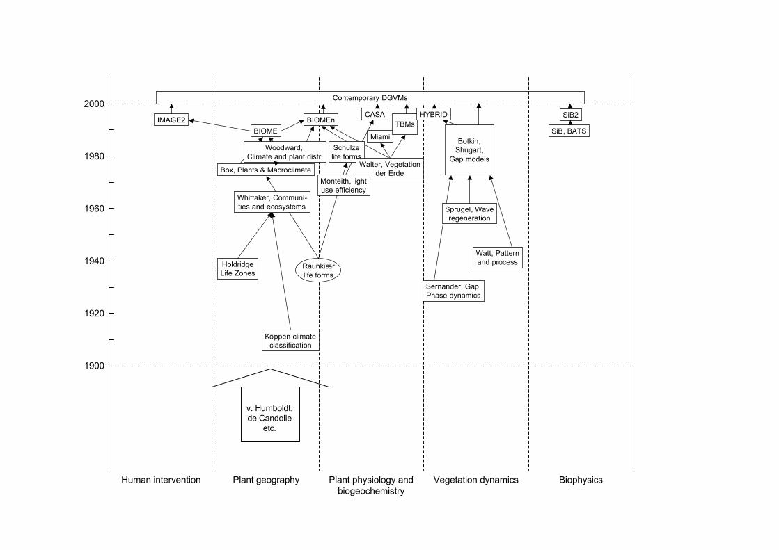
Schulzelife forms1980

Plant geography Plant physiology andbiogeochemistry

Vegetation dynamicsHuman intervention

1900

1920

1940

1960

2000

Köppen climateclassification

v. Humboldt,de Candolle

etc.

Miami

TBMs

Box, Plants & Macroclimate

HoldridgeLife Zones

Raunkiærlife forms

BIOME

BIOMEn

Sernander, Gap Phase dynamics

Sprugel, Waveregeneration

Botkin,Shugart,

Gap models

Contemporary DGVMs

IMAGE2

Biophysics

Whittaker, Communi-ties and ecosystems

CASA

Woodward, Climate and plant distr.

Walter, Vegetationder Erde

SiB, BATS

HYBRID

Watt, Patternand process

SiB2

Monteith, lightuse efficiency

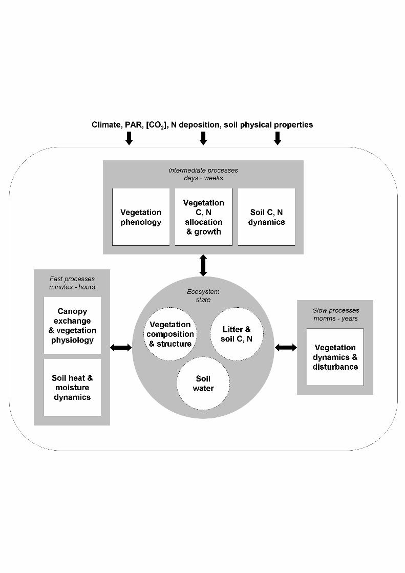
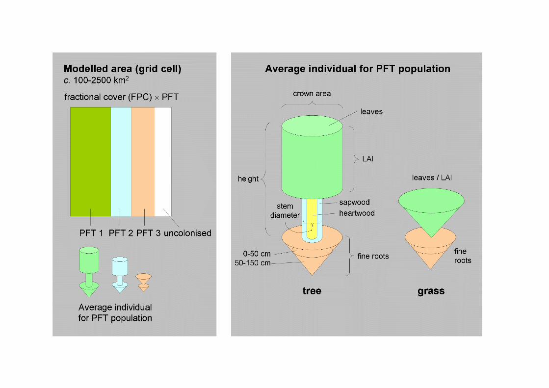
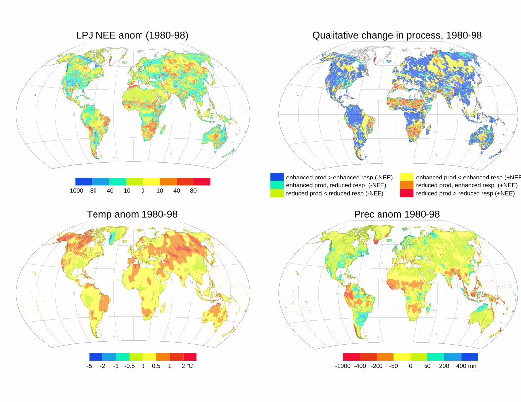
Qualitative change in process, 1980-98

enhanced prod > enhanced resp (-NEE)enhanced prod, reduced resp (-NEE)reduced prod < reduced resp (-NEE)

enhanced prod < enhanced resp (+NEEreduced prod, enhanced resp (+NEE)reduced prod > reduced resp (+NEE)

LPJ NEE anom (1980-98)

8040100-10-40-80-1000

Prec anom 1980-98

400 mm200500-50-200-400-1000

Temp anom 1980-98

2 °C10.50-0.5-1-2-5