Embed Size (px)
Citation preview
DEVELOPMENT AND ASSESSMENT OF AN X-RAY
FLUORESCENCE SYSTEM FOR IN VIVO STUDIES
by
WAN SALWANI JAAFAR
Thesis submitted in fulfilment of the requirements
for the Degree of Doctor of Philosophy
June 2009

ii
ACKNOWLEDGEMENTS
Praise is to Allah the Lord of the Universe.
It is a pleasure to acknowledge indebtedness to the many individuals that
made this study possible. First and foremost, I wish to express my sincere thanks to
my main supervisor, Professor Dr. Ahmad Shukri Mustapa Kamal for his kind
guidance, generous support, constant encouragement and invaluable advice over the
course of my study. My sincere thanks also go to my co-supervisor, Dr. Sabar Bauk
for his support, encouragement, helpful suggestions in working on the experiments
and also for his invaluable criticisms and suggestions right from the early drafts of
this thesis.
I would like to express my gratitude to Universiti Teknologi Mara for the
financial support throughout my study and also to the Dean, Faculty of Applied
Sciences, UiTM and the Campus Director, UiTM Perlis for their permission to
release me for my study leave.
I would like to thank the Dean and staff of the School of Physics, Universiti
Sains Malaysia for providing me with substantial support, most notably Mr. Azmi
Omar, Mr. Azmi Abdullah and Mr. Yahya for their technical assistance in the
laboratory and assuring that all my supplies was there when they were needed. I am
greatly indebted to my colleagues in UiTM Perlis; Professor Dr. Khudzir, Sabiha
Hanim, Assoc. Prof Zurina, Zaini and Rohaiza who shared with me their expertise in
analytical chemistry and Assoc. Prof. Norsila for the identification of the marine

iii
specimens. I also would like to thank current and former graduate students of the
Medical Physics group; especially to Dr Eid for sharing his expertise in the Monte
Carlo simulations and taking time to engage in open scientific discussions with me
and Dr Bassam for his guidance on using the X-ray generator during the initial stage
of experimentation. In addition, I would like to thank my friends; Aishah, Dr Rini
and Ramzun who could always be counted on for diversions and also for making my
life in the laboratory and my stay in the International House joyful.
Special thanks go to my parents, Jaafar and Wan Halimah for their
motivation, prayers and moral support and to my children; Firdaus, Nadiah, Faiz,
Najwa, Farhan and Nuha and also daughter-in-law, Nik Farhana for their
understanding and patience while mum was away from home. I also would like to
thank my siblings; Sakinah, Dr. Suhaimi, Salmiah, Saidi and Salmizi for their
encouragement throughout my study.
Finally, the greatest thanks go to my beloved husband, Mohamad Nadzam
Yaacob for giving me the permission to pursue my studies, for his love and
emotional support, for his patience and understanding, for his advices and
encouragement, and also for his sacrifices in taking the responsibility of the whole
family throughout this endeavour. This thesis is dedicated especially to him.
iv
TABLE OF CONTENTS
ACKNOWLEDGEMENTS ii
TABLE OF CONTENTS iv
LIST OF TABLES x
LIST OF FIGURES xii
LIST OF PLATES xvi
LIST OF SYMBOLS xvii
LIST OF ABBREVIATIONS xviii
LIST OF APPENDICES xx
LIST OF PUBLICATIONS & SEMINARS xxi
ABSTRAK xxii
ABSTRACT xxiv
CHAPTER ONE 1
INTRODUCTION 1
1.1 Introduction 1
1.2 Applications of X-ray Fluorescence 2
1.3 Scope of Work 3
1.4 Research Objectives 4
1.5 Thesis Organisation 5
v
CHAPTER TWO 6
THEORETICAL BACKGROUND 6
2.1 Introduction 6
2.2 Interactions of X-rays with Matter 6
2.2.1 Rayleigh Scattering 6
2.2.2 Compton Scattering 7
2.2.3 Photoelectric Absorption 8
2.2.4 Pair Production 11
2.3 Attenuation 12
2.4 Trace Elements 15
2.5 XRF for in vivo studies 16
2.6 Review of an XRF System 18
2.6.1 The Excitation Source 19
2.6.2 Measurement Geometry 22
2.6.3 Collimation and Shielding 23
2.6.4 Phantoms 24
2.6.5 Detectors 26
2.6.6 Dosimetry 28
2.7 Minimum Detectable Limits 29
2.8 Computer Simulations 31
2.8.1 Monte Carlo Methods 31
2.8.2 Applications of Monte Carlo Simulations for in vivo XRF
System 33
2.8.3 Monte Carlo N-Particle (MCNP) 34
2.8.4 Geometry Specifications of MCNP5 36
vi
2.8.5 The Input File 37
2.8.5(a) Cell Cards 38
2.8.5(b) Surface Cards 38
2.8.5(c) Data Cards 38
2.8.6 Simulations 39
2.8.7 The Output File 40
2.9 Conclusion 41
CHAPTER THREE 43
DEVELOPMENT OF THE XRF SYSTEM 43
3.1 Introduction 43
3.2 Set up with the Monte Carlo Method 43
3.2.1 Geometry Specifications 43
3.2.2 Data Cards 45
3.2.3 The Monte Carlo Simulations 47
3.3 Experimental Development 48
3.3.1 Excitation System 48
3.3.2 Detection System 51
3.3.2(a) Physical Characteristics of the Detector 52
3.3.3 Properties of the Calibration Source 53
3.3.4 Acquisition of Data 54
3.3.5 Analysis of Data 55
3.3.5(a) Statistical Error in Counting 55
3.3.6 Energy Calibration 57
3.3.7 Energy Resolution 59
3.3.8 Detection Efficiency 61
vii
3.3.9 Sample Preparation 64
3.3.10 Collimation and Shielding Assembly 67
3.3.11 XRF System Configuration 68
CHAPTER FOUR 71
OPTIMIZATION OF THE XRF SYSTEM 71
4.1 Introduction 71
4.2 Optimization by the Monte Carlo Method 72
4.2.1 Geometrical Optimization 73
4.2.1(a) Variation of the Source-to-Sample Distance (SSD) 73
4.2.1(b) Variation of the Sample-to-Detector Distance (SDD) 75
4.2.1(c) Variation of the Grazing Angle 76
4.2.2 Arsenic Content Calibration of the XRF System 78
4.2.3 Comparison of the Sensitivity and Minimum Detectable
Level 80
4.2.3(a) Variation of the SSD 80
4.2.3(b) Variation of the SDD 81
4.2.3(c) Variation of the Grazing Angle 82
4.3 Optimization by Experimentation 83
4.3.1 The Spectrum 84
4.3.2 Operating Voltage and Tube Current 86
4.3.3 Geometrical Optimization 88
4.3.3(a) Variation of the Grazing Angle 88
4.3.3(b) Variation of the SSD 89
4.3.3(c) Variation of the SDD 91
4.3.4 Arsenic Content Calibration of the XRF System 93
viii
4.4 Comparison of Simulations and Experimentation 95
4.5 Conclusion 97
CHAPTER FIVE 100
MULTI-ELEMENTAL ANALYSIS 100
5.1 Introduction 100
5.2 Elements Considerations 100
5.3 The Elements Selected 102
5.3.1 Chromium 103
5.3.2 Cobalt 103
5.3.3 Selenium 104
5.3.4 Strontium 104
5.3.5 Cadmium 105
5.4 Calibration of the XRF System for a Range of Elements 105
5.4.1 By Monte Carlo Methods 106
5.4.1(a) Different Operating Voltages 106
5.4.1(b) Identical Operating Voltage 109
5.4.1(c) Minimum Detectable Level of the Elements 111
5.4.2 By Experimentation 112
5.4.2(a) Preparation of Samples 113
5.4.2(b) Different Operating Voltages 115
5.4.2(c) Identical Operating Voltages 117
5.4.2(d) Minimum Detectable Level of the Elements 122
5.5 Minimum Detectable Level: Simulations versus Experimentation 122
5.6 Multi-elemental Analysis 123
5.6.1 Dual Elements 124
ix
5.6.2 Multiple Elements 127
5.7 Application of Multi-elemental Analysis 129
5.8 The Marine Samples 130
5.9 Multi-elemental Analysis with the XRF System 133
5.9.1 Experimental Procedures 133
5.9.2 Spectra of the Marine Samples 133
5.9.3 Elemental Concentration Analysis 139
5.10 Multi-elemental Analysis with Neutron Activation Analysis 142
5.11 Comparison of Concentration for Common Elements 143
5.12 Elemental Concentrations for Marine Species in other Studies 145
5.13 Conclusion 149
CHAPTER SIX 151
CONCLUSION 151
6.1 Summary 151
6.2 Future Work 153
REFERENCES 166
x
LIST OF TABLES Table 2.1: The MCNP5 Input file structure. 37
Table 3.1: The most abundant -rays produced in the decay of 241Am. 54
Table 3.2: The photo peaks of 241Am and several metal plates. 58
Table 3.3: The energy resolution of the LEGe detector. 61
Table 3.4: Physical and chemical properties of arsenic pentoxide. 65
Table 3.5: The properties of arsenic and its X-ray energies. 66
Table 4.1: Range of values of the variables studied. 84
Table 4.2: Concentration of arsenic. 93
Table 5.1: Elements of interest. 102
Table 5.2: The properties of the selected elements and its X-ray
energies. 103
Table 5.3: Minimum detectable level of the elements by simulations. 112
Table 5.4: Physical and chemical properties of the substances used. 113
Table 5.5: Solution concentration. 114
Table 5.6: Minimum detectable level of the elements by
experimentation. 122
Table 5.7: Comparison of counts in individual and combined samples. 126
Table 5.8: Comparison of measured and actual concentrations of the
elements in dual samples. 127
Table 5.9: Comparison of counts in individual and multiple samples. 128
Table 5.10: Comparison of measured and actual concentrations of the
elements in multiple samples. 129
Table 5.11: The classifications of the marine samples. 131
Table 5.12: As, Se, Sr and Cd in marine samples by XRF. 140
xi
Table 5.13: Action Levels, Tolerances and Guidance Levels for Toxic
Elements in Seafood 141
Table 5.14: Element concentrations in marine samples by NAA. 143
Table 5.15: As, Se, Sr and Cd concentrations in different species
reported as means or range of concentrations from
regions in various parts of the world. 147
xii
LIST OF FIGURES
Figure 2.1: Illustrative summary of (A) Rayleigh scattering and (B)
Compton scattering. 7
Figure 2.2: Photoelectric absorption. 9
Figure 2.3: Fluorescence X-ray emission of (A) K and (B) K. 9
Figure 2.4: Auger electron emission. 10
Figure 2.5: Energy level diagram and electronic transition. 11
Figure 2.6: Illustration of pair production. 12
Figure 3.1: Cross-sectional x-y view of the geometrical setting. 44
Figure 3.2: The pulse height distributions for 600 g/g As obtained
using the Monte Carlo code. 48
Figure 3.3: A schematic representation of the X-ray beam profile
experiments setup. 49
Figure 3.4: A schematic representation of the X-ray beam image on a
film. 50
Figure 3.5: Variations of X-ray beam diameter with distance of image
from the collimator. 50
Figure 3.6: Variations of X-ray beam height with distance of image
from the X-ray aperture. 51
Figure 3.7: (A) Cross-section of the LEGe detector and (B) the
detector chamber. 53
Figure 3.8: A schematic diagram of the data acquisition system. 55
Figure 3.9: Probability P(N) as a function of N and . 57
Figure 3.10: Photon spectrum of 241Am recorded with the LEGe
detector. 58
Figure 3.11: Energy calibration for the LEGe detector. 59
xiii
Figure 3.12: Definition of detector resolution. 60
Figure 3.13: Energy resolution for the LEGe detector. 61
Figure 3.14: Solid angle subtended by the detector at the source
position. 62
Figure 3.15: The intrinsic efficiency curve for the LEGe detector. 64
Figure 3.16: The schematic system components of the experimental
XRF system. 68
Figure 3.17: Variation of dead time of the detector to sample angle. 70
Figure 4.1: Variation of XRF counts with SSD. 74
Figure 4.2: Variation of the percentage of particles entering the
detector to that entering the sample with the SSD. 74
Figure 4.3: Variation of XRF counts with SDD. 75
Figure 4.4: Variation of the percentage of particles entering the
detector to that entering the sample with the SDD. 76
Figure 4.5: Variation of XRF counts with the grazing angle. 77
Figure 4.6: Variation of the percentage of particles entering the
detector to that entering the sample with grazing angle. 77
Figure 4.7: Illustration of sample area irradiated by the source. 78
Figure 4.8: Calibration line of arsenic. 79
Figure 4.9: Effect of different SSD on the sensitivity and MDL. 81
Figure 4.10: Effect of different SDD on the sensitivity and MDL. 82
Figure 4.11: Effect of different sample angle on the sensitivity and
MDL. 83
Figure 4.12: A typical spectrum of the sample. 85
Figure 4.13: A typical fit to the arsenic response peak using PeakFit. 86
Figure 4.14: Variation of counts with tube current for different
operating voltage. 87
xiv
Figure 4.15: Variation of counts-to-background ratio with tube current
for different operating voltage. 88
Figure 4.16: Variation of counts with grazing angle. 89
Figure 4.17: Variation of the arsenic peak area with distance from the
sample to the excitation source. 91
Figure 4.18: Representation of the X-ray beam incident on a sample
with a smaller source-to-detector distance in (A)
compared to that in (B). 91
Figure 4.19: Variation of the arsenic peak area with distance from the
sample to the detector. 92
Figure 4.20: Variations in the 10.5 keV peak due to differing arsenic
concentrations. 94
Figure 4.21: The calibration curve of arsenic. 95
Figure 4.22: Variation of normalized counts with SSD. 96
Figure 4.23: Variation of normalized counts with grazing angle. 97
Figure 5.1: Calibration curves of (A) Cr at 30 kVp, (B) Co at 30 kVp,
(C) Se at 35 kVp, (D) Sr at 45 kVp and (E) Cd at 45
kVp. 108
Figure 5.2: Calibration curves of (A) Cr, (B) Co, (C) As and (D) Se
with an identical operating voltage of 45 kVp. 110
Figure 5.3: Variation of sensitivity at 45 kVp for a range of elements. 111
Figure 5.4: Variation of MDL for a range of elements. 112
Figure 5.5: Calibration curves of (A) Cr at 20 kVp, (B) Co at 25 kVp,
(C) Se at 40 kVp, (D) Sr at 45 kVp and (E) Cd at 45
kVp. 117
Figure 5.6: A typical spectrum of (A) Cr, (B) Co, (C) As, (D) Se, (E)
Sr and (F) Cd with an identical operating voltage of 45
kVp. 119
xv
Figure 5.7: Calibration curves of (A) Cr, (B) Co, (C) As and (D) Se
with an identical operating voltage of 45 kVp. 121
Figure 5.8: MDL as a function of the atomic number of the elements. 123
Figure 5.9: Typical spectra for samples containing (A) Cr and Co, (B)
As and Se and (C) Sr and Cd. 125
Figure 5.10: Typical spectrum for a sample containing all six
elements. 127
Figure 5.11: The typical XRF spectra of the banana prawn samples:
(A) PR11, (B) PR12 and (C) PR13. 134
Figure 5.12: The typical XRF spectra of the blood cockle samples: (A)
CK11, (B) CK12 and (C) CK13. 135
Figure 5.13: The typical XRF spectra of the carpet clam samples: (A)
MS11, (B) MS12 and (C) MS13. 136
Figure 5.14: The typical XRF spectra of other clam samples: (A)
CL11, (B) CL12 and (C) CL13. 137
Figure 5.15: The typical XRF spectra of the sea cucumber samples:
(A) SC11, (B) SC12 and (C) SC13. 138
Figure 5.16: Radiative capture. 142
Figure 5.17: Comparison of As concentration 144
Figure 5.18: Comparison of Se concentration 144
xvi
LIST OF PLATES Plate 3.1: The XRF system setup in the Biophysics Lab. 67
Plate 5.1: The marine samples used were (A) banana prawns, (B)
blood cockles, (C) carpet clams, (D) other clams and (E)
sea cucumbers. 132

xvii
LIST OF SYMBOLS alpha
beta
gamma
theta
phi
micro
m milli
k kilo
decay constant
Z atomic number
A mass number
standard deviation
density
0E incident photon energy
BEE binding energy
SE scattered photon energy
l linear attenuation coefficient
m mass attenuation coefficient
xviii
LIST OF ABBREVIATIONS
Bq becquerel
CdTe cadmium telluride
CdZnTe cadmium zinc telluride
EGS electron gamma shower
ETRAN electron transport
eV electron volt
GHz gigahertz
Gy gray
HVL half value layer
HPGe high purity germanium
ITS integrated tiger system
IAEA International Atomic Energy Agency
kVp kilovolt peak voltage
Ge(Li) lithium drifted germanium
Si(Li) lithium drifted silicon
L litre
LEGe low energy germanium
MDL minimum detectable limit
HgI mercury iodide
MCNP Monte Carlo N-Particle
MCNP5 Monte Carlo N-Particle version 5
NAA neutron activation analysis
ppm parts-per-million

xix
RAM random access memory
SDD sample-to-detector distance
Sv sievert
NaI(Tl) sodium iodide thallium
SSD source-to-sample distance
sr steradian
XRF X-ray fluorescence

xx
LIST OF APPENDICES Appendix A: The input file for the Monte Carlo simulations of arsenic
concentration of 600 g/g with a grazing angle at 45°. 155
Appendix B: The activity of 241Am. 158
Appendix C: The intrinsic peak efficiency of the LEGe detector. 159
Appendix D: The error analysis for the intrinsic peak efficiency 160
Appendix E: The stock solution of orthoarsenic acid. 162
Appendix F: The reference solutions of orthoarsenic acid. 164
Appendix G: The arsenic concentration. 165
xxi
LIST OF PUBLICATIONS & SEMINARS
Jaafar, W. S. and Shukri, A., 2006. Monte Carlo Simulations for in vivo Analysis of
Arsenic Using X-Ray Fluorescence. In: 5th National Seminar on Medical Physics:
Globalization of Physics in Health and Medical Sciences. Kuala Lumpur, Malaysia
14-15 December 2006. Malaysian Association of Medical Physics: Kuala Lumpur.
Jaafar, W. S. and Shukri, A., 2006. Monte Carlo Simulations for in vivo Analysis of
Arsenic Using X-Ray Fluorescence, NSMP 2006 Proceedings, pp.68-74.
xxii
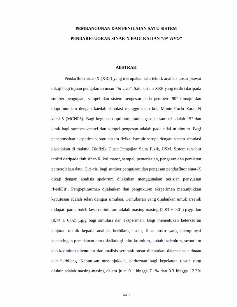
PEMBANGUNAN DAN PENILAIAN SATU SISTEM
PENDARFLUORAN SINAR-X BAGI KAJIAN “IN VIVO”
ABSTRAK
Pendarfluor sinar-X (XRF) yang merupakan satu teknik analisis unsur piawai
dikaji bagi tujuan pengukuran unsur “in vivo”. Satu sistem XRF yang terdiri daripada
sumber pengujaan, sampel dan sistem pengesan pada geometri 90° dimaju dan
dioptimumkan dengan kaedah simulasi menggunakan kod Monte Carlo Zarah-N
versi 5 (MCNP5). Bagi kegunaan optimum, sudut geselan sampel adalah 15° dan
jarak bagi sumber-sampel dan sampel-pengesan adalah pada nilai minimum. Bagi
penentusahan eksperimen, satu sistem fizikal hampir serupa dengan sistem simulasi
disediakan di makmal Biofizik, Pusat Pengajian Sains Fizik, USM. Sistem tersebut
terdiri daripada tiub sinar-X, kolimator, sampel, pemerisaian, pengesan dan peralatan
pemerolehan data. Ciri-ciri bagi sumber pengujaan dan pengesan pendarfluor sinar-X
dikaji dengan analisis spektrum dilakukan menggunakan perisian penyuaian
‘PeakFit’. Pengoptimuman dijalankan dan pengukuran eksperimen menunjukkan
keputusan adalah selari dengan simulasi. Tentukuran yang dijalankan untuk arsenik
didapati paras boleh kesan minimum adalah masing-masing (2.83 0.01) g/g dan
(0.74 0.02) g/g bagi simulasi dan eksperimen. Bagi menentukan ketersauran
lanjutan teknik kepada analisis berbilang unsur, lima unsur yang mempunyai
kepentingan pemakanan dan toksikologi iaitu kromium, kobalt, selenium, strontium
dan kadmium ditentukur dan analisis serentak unsur ditentukan dalam unsur duaan
dan berbilang. Keputusan menunjukkan, perbezaan bagi kepekatan unsur yang
diukur adalah masing-masing dalam julat 0.1 hingga 7.1% dan 0.3 hingga 12.3%
xxiii
bagi unsur duaan dan berbilang dibandingkan dengan sampel satu unsur. Bagi
melanjutkan penilaian keupayaan teknik tersebut, analisis unsur dalam invertebrat
marin Malaysia umum dijalankan. Keputusan bagi kepekatan arsenik dan selenium
adalah dalam magnitud yang sama dibandingkan dengan yang didapati melalui
teknik Analisis Pengaktifan Neutron (NAA). Julat kepekatan bagi arsenik, selenium,
strontium dan kadmium yang diperolehi adalah sebanding dengan yang diperolehi
bagi spesis marin dari kajian literatur yang lain.
xxiv
DEVELOPMENT AND ASSESSMENT OF AN X-RAY FLUORESCENCE
SYSTEM FOR IN VIVO STUDIES
ABSTRACT
X-ray fluorescence (XRF), which is a standard elemental analysis technique,
was investigated for the purpose of measuring elements in vivo. An XRF system
comprising of an excitation source, sample and a detection system in a 90° geometry
was developed and optimized by simulations using the Monte Carlo code, Monte
Carlo N-Particle version 5 (MCNP5). For optimal use, the grazing angle of the
sample is at 15° and the source-to-sample distance (SSD) and sample-to-detector
distance (SDD) were at minimum values. For experimental verification, a physical
system almost similar to the simulated system was set up at the Biophysics
Laboratory, School of Physics, USM. The system comprises of an X-ray tube,
collimators, sample, shielding, a detector and data acquisition equipments. The
characteristics of the excitation source and the fluorescent X-ray detector were
investigated with spectral analysis performed using the PeakFit fitting software.
Optimizations were carried out and experimental measurements showed that the
results agreed with that obtained by simulations. Calibration for arsenic was
performed with the minimum detectable level by simulation and experimentation
determined to be (2.83 0.01) g/g and (0.74 0.02) g/g respectively. To
determine the feasibility of extending the technique to multi-elemental analysis;
another five elements of nutritional and toxicological interest, namely chromium,
cobalt, selenium, strontium and cadmium were calibrated and then simultaneously
determined in dual and multi-elemental analysis. Results showed that, compared to
single element samples, the differences of the measured concentrations of the
xxv
elements ranges from 0.1 to 7.1% and 0.3 to 12.3% in dual and multi-elemental
samples respectively. To further evaluate the capacity of the technique, analysis of
the elements in common Malaysian marine invertebrates were performed. Results for
arsenic and selenium concentrations as compared with that obtained from another
technique, Neutron Activation Analysis (NAA) showed that the concentrations were
within the same order of magnitude. The ranges of arsenic, selenium, strontium and
cadmium concentrations obtained were comparable to that obtained for marine
species in other studies in the literature.
1
CHAPTER ONE
INTRODUCTION
1.1 Introduction
XRF has become a powerful and portable analytical tool in many fields.
Fluorescence, or the generation of secondary radiation, is accomplished by a two-
step process. In the first step, a high energy particle such as a photon, a proton or an
electron strikes an atom and knocks out an inner-shell electron (photoelectric effect).
The second step is readjustment in the atom almost immediately (10-12 to 10-14 s) by
filling the inner-shell vacancy with one of the outer-shell electrons and the
simultaneous emission of an X-ray photon. The first step uses up the energy of the
incident quantum, and in the second step energy is emitted as the characteristic X-ray
photon.
The technology works by irradiating samples of materials using X-rays
without destroying the analysed material. The material emits radiation, which has an
energy characteristic of the atoms present. Analysis by XRF consists of determining
the content of specific elements in a sample by producing vacancies in the electronic
structures and analysing the photons emitted as a consequence. At the same time, it
can identify a vast number of elements simultaneously, making it an excellent way to
"fingerprint" all kinds of materials.

2
1.2 Applications of X-ray Fluorescence
The great flexibility and range of the various types of X-ray spectrometers
coupled with the development in X-ray detectors has established the XRF method as
a powerful technique in a number of applications, including:
a) Geology and mineralogy; for the analysis of minerals (Pinetown et al., 2007,
Siyanbola et al., 2004), rocks (Tarasov et al., 1998), ore (Devan et al., 1997,
Herrera Peraza et al., 2004), soils (Mc Donald et al., 1999), silts and
sediments (Zachara et al., 2004) and the heavy metals measurement in rock
phosphates (Hayumbu et al., 1995).
b) Ecology and environmental management; for the analysis of aerosols (Devan
et al., 1997); pollution of water (Marques et al., 2003), soil (Krishna and
Govil, 2007) and air particle (Suarez et al., 2004); lead monitoring in lead-
based industrial areas (Herman et al., 2006) and soil samples (Markey et al.,
2008); and the assessment of marine pollution (Woelfl et al., 2006) and heavy
metals in lake sediments (de Vives et al., 2007).
c) Archaeology and forensics; in the analysis of ancient pottery
(Papachristodoulou et al., 2006), Chinese jades (Casadio et al., 2007),
ceramics (Cechak et al., 2007), porcelain (Yu and Miao, 1997) and glass
(Jembrih-Simburger et al., 2004); metal artifacts (Araujo et al., 2004, Fikrle
et al., 2006) and coins (Linke et al., 2004); human bones of ancient
populations (Rebocho et al., 2006) and the investigation of paintings
(Szokefalvi-Nagy et al., 2004) and other works of art (Cesareo et al., 1999).
d) Industry; for the analysis of trace elements in a metal matrix for the
assessment of radiation damage of core components in a nuclear power plant
(van Aarle et al., 1999), elemental composition of chromites ore in the
3
ceramic industry (Sanchez-Ramos et al., 2008), elemental analysis in
lubricants (Schramm, 2002), determination of wear metals in engine oil
(Yang et al., 2003) and used lubricating oils (Arikan et al., 1996),
concentration of sulphur in the products of the petroleum industry
(Christopher et al., 2001, Miskolczi et al., 2005) and the analysis of trace
elements in coal (Suarez-Fernandez et al., 2001), waste material (Akinci and
Artir, 2008) and cement factory raw material (Polat et al., 2004).
e) Clinical and biological; for in vivo studies such as measurement of lead in
bone (Somervaille et al., 1985); studies on aquatic species such as the
analysis of muscles and livers of freshwater fish (Wagner and Boman, 2004),
studies on how metals accumulate and redistribute during fertilization and
embryonic developments of the African clawed frog (Popescu et al., 2007);
studies of plants (Richardson et al., 1995), mushrooms (Carvalho et al.,
2005), plants having medicinal properties (Ekinci et al., 2004) and plant
materials such as the analysis of fruit juice (Bao et al., 1999) and spices (Al-
Bataina et al., 2003, Jayasekera et al., 2004).
1.3 Scope of Work
XRF has been an established technique for the measurement of toxic and
essential trace elements in vivo (Borjesson et al., 1998, Chettle, 2005). This study
involves the designing, developing and assessing of an XRF system and will be
restricted to applications for in vivo studies.
With the help of faster computers, simulation is becoming more and more
important in many fields of design and analysis due to the several advantages of

4
simulations compared to experimental studies. Taking this into account, computer
simulations, particularly the Monte Carlo N-Particle version 5 (MCNP5) code will be
used. Different parameters in the simulation will be changed and the effect of these
changes on the performance of the XRF system will be investigated. The system will
be optimized and calibrated by using both computer simulations and experimental
methods.
1.4 Research Objectives
The objective of this research is to use computer simulations and
experimental analysis to examine photon interactions associated with in vivo XRF
measurement of arsenic. This investigation is designed to determine the feasibility of
extending the technique of XRF of arsenic to multi-elemental analysis of another five
elements particularly, chromium, strontium, cadmium, cobalt and selenium where
their atomic number, Z ranges from Z = 24 to Z = 48.
During the course of the investigation attempts were made:
a. To develop an arsenic XRF system with Monte Carlo simulation and
experimental verification.
b. To calibrate the X-ray intensity with concentration for arsenic and the other
elements by both methods.
c. To acquire information concerning the feasibility of obtaining concentration
for two elements and six elements simultaneously for in vivo measurements
and
d. To apply the XRF system to determine the concentration of elements of
interest in common Malaysian marine invertebrates in vivo and to compare
5
with those obtained by using the method of neutron activation analysis
(NAA).
1.5 Thesis Organisation
In this thesis, an XRF system with the potential for in vivo studies is
presented. The XRF system was developed and optimized by computer simulations
using the Monte Carlo N-Particle Version 5 (MCNP5) code and also by
experimentation.
Appropriate parameters had to be identified and understood in terms of how
the parameters affect the output counts of the XRF system. With this in mind,
Chapter 2 contains the theoretical background and characterisation parameters which
are related and important to the XRF system. The descriptions about MCNP5 which
are relevant to the system are also presented. Chapter 3 contains a description of the
characteristics of each component of the XRF system and Chapter 4 contains a
description of how those parameters were optimized by both MCNP5 and
experimentation and also the calibration of the XRF system for arsenic. Chapter 5
contains the extension of the XRF system for five other elements of interest which
includes elemental calibration and the analysis of two and six elements
simultaneously. The application of multi-elemental analysis on common Malaysian
marine invertebrates was described and with the analysis of data obtained, the
elements concentrations were evaluated. Comparisons made with the method of
neutron activation analysis showed that the XRF system has the potential to be used
for in vivo studies.
6
CHAPTER TWO
THEORETICAL BACKGROUND
2.1 Introduction
X-rays are electromagnetic radiation with their region lying between 0.01 and
10 nm (0.1 to 100 keV) in the electromagnetic spectrum, that is between the -
region at the short-wavelength or high-energy side and the ultraviolet region at the
long-wavelength or low-energy side. However, these boundaries are not clearly
defined.
2.2 Interactions of X-rays with Matter
When a beam of X-ray photons passes into an absorbing medium, the process
of collision between one photon and some electrons in the medium produces
scattered radiation and the setting in motion of a high speed electron. The process of
interaction is by four distinct mechanisms known as Rayleigh scattering, Compton
scattering, photoelectric absorption and pair production.
2.2.1 Rayleigh Scattering
An incident X-ray photon can interact with an electron and be deflected
(scattered) with no loss of energy. The process which is also known as coherent or
elastic scattering occurs by temporarily raising the energy of the electron although
the electron remains bound to the nucleus. The electron returns to its initial energy
level by emitting an X-ray photon of equal energy but with a slightly different
direction, as illustrated in Figure 2.1A. No ionisation takes place and no energy is
lost in Rayleigh scattering. Rayleigh scattering occurs at all X-ray energies, however
7
it never accounts for more that 10% of the total interaction processes in diagnostic
radiology (Dendy and Heaton, 2000). This type of scattering is dependent
approximately on 2Z and of importance in analytical X-ray fluorescence because of
its contribution to the general background (Biran-Izak and Mantel, 1994).
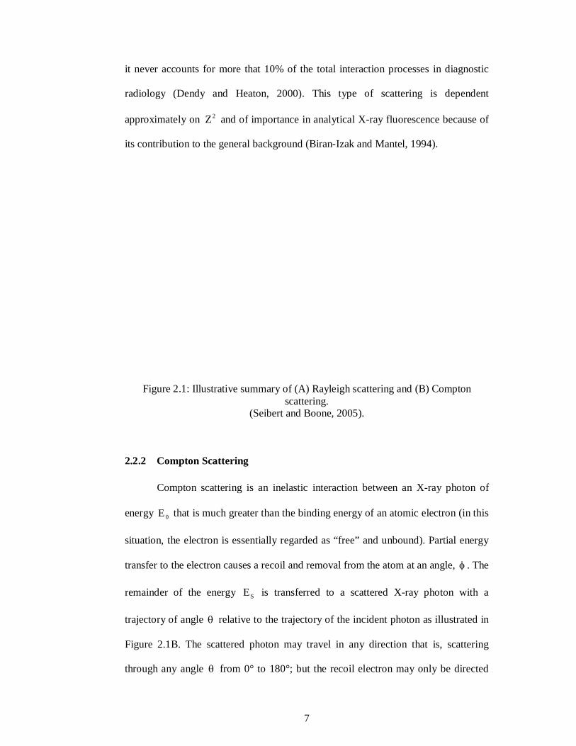
Figure 2.1: Illustrative summary of (A) Rayleigh scattering and (B) Compton scattering.
(Seibert and Boone, 2005).
2.2.2 Compton Scattering
Compton scattering is an inelastic interaction between an X-ray photon of
energy 0E that is much greater than the binding energy of an atomic electron (in this
situation, the electron is essentially regarded as “free” and unbound). Partial energy
transfer to the electron causes a recoil and removal from the atom at an angle, . The
remainder of the energy SE is transferred to a scattered X-ray photon with a
trajectory of angle relative to the trajectory of the incident photon as illustrated in
Figure 2.1B. The scattered photon may travel in any direction that is, scattering
through any angle from 0° to 180°; but the recoil electron may only be directed
8
forward relative to the angle of the incident photon that is the angle lies from 0° to
~90°. Due to the physical requirements to preserve both energy and momentum, the
energy of the scattered photon relative to the incident photon for a photon scattering
angle is given by the Compton relations:
cos1
keV511E
1
1EE
00
S (2.1)
where 511 keV is the energy equal to the rest mass of the electron and 0E and SE
are in keV.
Compton scattering is independent of atomic number and it decreases with
increase in energy. The most important consequence of Compton scattering is the
appearance of scattered photons of lower energy than the incident photon beam,
which may cause overlap and high background effects in the XRF spectra.
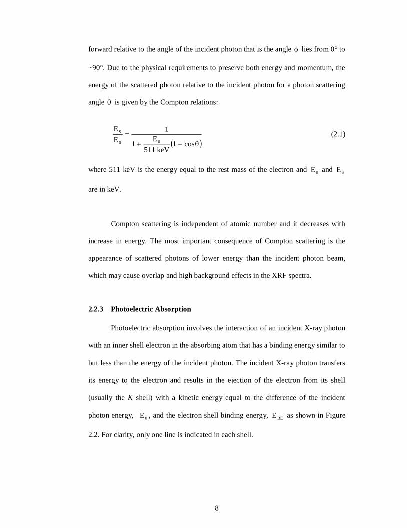
2.2.3 Photoelectric Absorption
Photoelectric absorption involves the interaction of an incident X-ray photon
with an inner shell electron in the absorbing atom that has a binding energy similar to
but less than the energy of the incident photon. The incident X-ray photon transfers
its energy to the electron and results in the ejection of the electron from its shell
(usually the K shell) with a kinetic energy equal to the difference of the incident
photon energy, 0E , and the electron shell binding energy, BEE as shown in Figure
2.2. For clarity, only one line is indicated in each shell.
9
Figure 2.2: Photoelectric absorption. (Als-Nielsen and Mc Morrow, 2001).
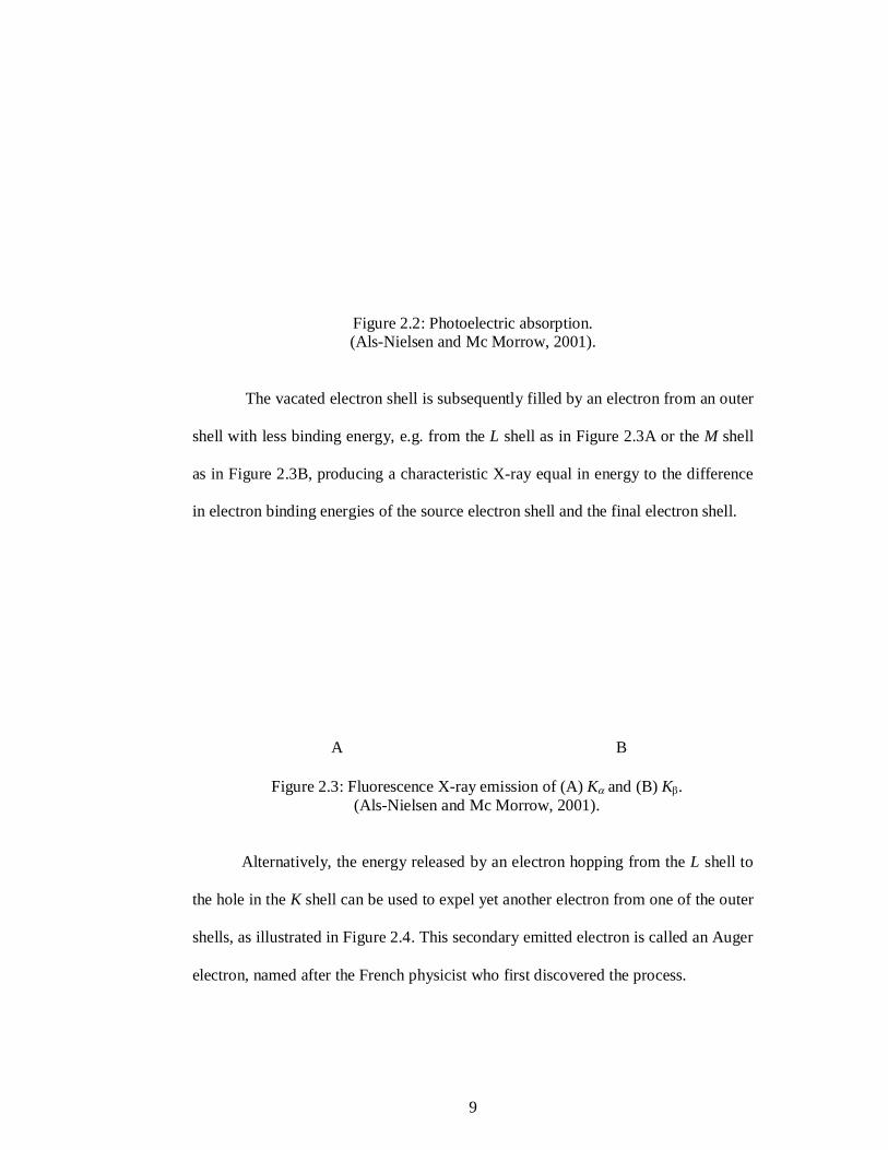
The vacated electron shell is subsequently filled by an electron from an outer
shell with less binding energy, e.g. from the L shell as in Figure 2.3A or the M shell
as in Figure 2.3B, producing a characteristic X-ray equal in energy to the difference
in electron binding energies of the source electron shell and the final electron shell.
A B
Figure 2.3: Fluorescence X-ray emission of (A) K and (B) K. (Als-Nielsen and Mc Morrow, 2001).
Alternatively, the energy released by an electron hopping from the L shell to
the hole in the K shell can be used to expel yet another electron from one of the outer
shells, as illustrated in Figure 2.4. This secondary emitted electron is called an Auger
electron, named after the French physicist who first discovered the process.

10
Figure 2.4: Auger electron emission. (Als-Nielsen and Mc Morrow, 2001).
If the incident photon energy is less than the binding energy of the electron,
the photoelectric interaction cannot occur, but if the X-ray energy is equal to the
electronic binding energy )EE( BE0 , the photoelectric effect becomes energetically
feasible and a large increase in attenuation occurs. As the incident photon energy
increases above that of the electron shell binding energy, the likelihood of
photoelectric absorption decreases at a rate proportional to 3E .
The K absorption edge refers to the sudden jump in the probability of
photoelectric absorption when the K-shell interaction is energetically possible.
Similarly, the L absorption edge refers to the sudden jump in photoelectric absorption
occurring at the L-shell electron binding energy (at much lower energy). Actually,
the K absorption edge is approximately the sum of the K, L and M line energies, and
the L absorption edge energy is approximately the sum of the L and M line energies
of the particular element.
The characteristic X-rays are labelled as K, L or M to denote the shells they
originated from. The designations , or is made to mark the X-rays that
originated from the transitions of electrons from the higher shells. Hence, a K X-ray
11
is produced from a transition of an electron from the L to the K shell, and a K X-ray
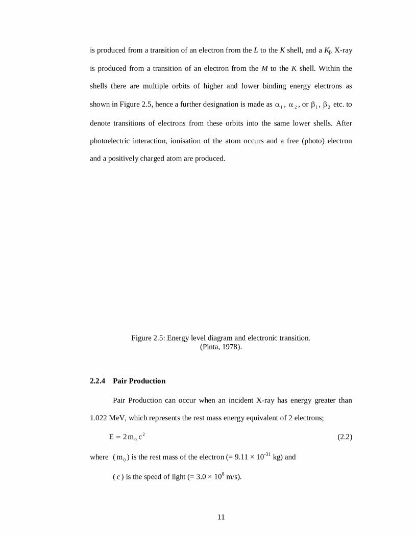
is produced from a transition of an electron from the M to the K shell. Within the
shells there are multiple orbits of higher and lower binding energy electrons as
shown in Figure 2.5, hence a further designation is made as 1 , 2 , or 1 , 2 etc. to
denote transitions of electrons from these orbits into the same lower shells. After
photoelectric interaction, ionisation of the atom occurs and a free (photo) electron
and a positively charged atom are produced.
Figure 2.5: Energy level diagram and electronic transition. (Pinta, 1978).
2.2.4 Pair Production
Pair Production can occur when an incident X-ray has energy greater than
1.022 MeV, which represents the rest mass energy equivalent of 2 electrons;
20 cm2E (2.2)
where ( 0m ) is the rest mass of the electron (= 9.11 × 10⁻³¹ kg) and
( c ) is the speed of light (= 3.0 × 10⁸ m/s).
12
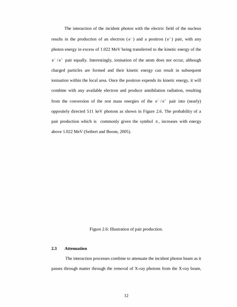
The interaction of the incident photon with the electric field of the nucleus
results in the production of an electron ( e ) and a positron ( e ) pair, with any
photon energy in excess of 1.022 MeV being transferred to the kinetic energy of the
e/e pair equally. Interestingly, ionisation of the atom does not occur, although
charged particles are formed and their kinetic energy can result in subsequent
ionisation within the local area. Once the positron expends its kinetic energy, it will
combine with any available electron and produce annihilation radiation, resulting
from the conversion of the rest mass energies of the e/e pair into (nearly)
oppositely directed 511 keV photons as shown in Figure 2.6. The probability of a
pair production which is commonly given the symbol , increases with energy
above 1.022 MeV (Seibert and Boone, 2005).
Figure 2.6: Illustration of pair production.
2.3 Attenuation
The interaction processes combine to attenuate the incident photon beam as it
passes through matter through the removal of X-ray photons from the X-ray beam,
13
therefore decreasing its intensity, either by absorption or scattering events. The
amount of decrease in intensity of the X-ray beam depends upon the depth of
penetration or thickness, x and linear attenuation coefficient, l which is a
characteristic of the material, that is
x0
leII (2.3)
where ( 0I ) and ( I ) are the initial and final X-ray beam intensities respectively.
The unit of thickness is commonly expressed in cm, so the corresponding unit of l
is cm-1, and l represents the probability of attenuation per cm of a material. The
total linear attenuation coefficient is the sum of the linear attenuation coefficients for
the individual interaction mechanisms, as
total = PE + CS + RS + PP (2.4)
total photoelectric effect Compton
scattering Rayleigh scattering Pair
production
At low X-ray energy, PE dominates and 34 EZ ; at high energy, CS
dominates and and only at very high energy, that is greater than 1.022 MeV
does PP contribute. Therefore, interaction by pair-production does not occur in this
study because the X-ray energy used is very much lower than 1.022 MeV. At a given
photon energy, the linear attenuation coefficient can vary significantly for the same
material if it exhibits differences in physical density. A classical example is water,
water vapour and ice. The mass attenuation coefficient,
lm (2.5)
14
compensated for these variations by normalising the linear attenuation by the density
of the material, . In terms of m , Equation 2.3 now becomes
x0
meII (2.6)
An interesting application of Equation 2.6 is to determine the depth of
penetration of X-rays. The attenuation length is defined as the depth into the material
where the intensity of the X-rays has decreased to about 37% or e1 of its value at the
surface. That is, 0Ie1I
, or
e1
II
0
where ( e ) sometimes called Euler's number
or Napier's constant, is the base of natural logarithms, or e ≈ 2.7183. Then,
substituting into Equation 2.6;
xe1ln m
x1 m
Hence
m
1x (2.7)
where ( x ) is also referred to as the “mean free path” of the X-rays. The mean free
path is, as the name suggests, the average distance travelled by a photon before
undergoing some form of interaction.
X-ray beams have a spectral distribution of energies. Hence a rule of thumb is
often used which states that the average X-ray energy is approximately one-third of
the maximum energy or kVp (Khan, 1984). Therefore, for an operating voltage of 45

15
kVp which has been used as the identical operating voltage and described in Section
5.4.2(c), the average energy is approximately 15 keV. For soft tissue (ICRU Four-
Component) of density, = 1 g/cm3 and the mass attenuation coefficient at 15 keV
is m = 1.266 cm2/g (N.I.S.T., 2005); plugging in the numbers into Equation 2.7, the
mean free path, x = 0.79 cm.
2.4 Trace Elements
Some metals are naturally found in the body and are essential to human
health. They normally occur at low concentrations and are known as trace metals. In
high doses, they may be toxic to the body or produce deficiencies in other trace
metals; for example, high levels of zinc can result in a deficiency of copper, another
metal required by the body. Heavy or toxic metals are trace metals with a density at
least five times that of water. As such, they are stable elements which mean that they
cannot be metabolised by the body and they are bio-accumulative, that is, they
passed up the food chain to humans. Once liberated into the environment through the
air, drinking water, food, or countless human-made chemicals and products, heavy
metals are taken into the body via inhalation, ingestion and skin absorption. If heavy
metals enter and accumulate in body tissues faster than the body’s detoxification
pathways can dispose them, a gradual build-up of these toxins will occur. High-
concentration exposure is not necessary to produce a state of toxicity in the body as
heavy metals accumulate in body tissues and over time can reach toxic concentration
levels. Thus there is a need to control their levels in human organs and tissues
especially for occupationally and environmentally highly exposed persons. The
distribution of trace elements within the body is often very non-uniform and are
16
usually found in specific organs such as iodine in the thyroid, lead in bone and
cadmium and mercury in kidney cortex, etc.
2.5 XRF for in vivo studies
There are two main non-invasive techniques for in vivo studies, namely the
XRF and neutron activation analysis (NAA). Compared to NAA, XRF has the
advantage of being non-destructive, multi-elemental, fast and cost-effective. The
analysis is said to be non-destructive in the sense that, at the end of it, most of the
elements originally present in the sample are still there and chemically unchanged.
The sample is therefore; to some extent available for further study should this be
considered necessary or desirable.
The first XRF measurement in vivo was performed to measure iodine levels
in the thyroid gland (Hoffer et al., 1968). However, the most recognised and applied
XRF technique is bone lead XRF measurements in humans. Measurements of lead in
vivo began in 1971 (Ahlgren et al., 1976, Ahlgren and Mattsson, 1979) using 122
and 136 keV photons from 57Co for excitation of the lead K X-rays and a similar
technique has also been used to estimate the lead concentration in children’s teeth in
situ (Bloch et al., 1976). There are four different approaches for bone lead
measurements which have been developed, namely:
a. A 109Cd source that induces K XRF of lead stored in the tibia or some other
bone was employed in a backscatter geometry (Green et al., 1993,
Kondrashov and Rothenberg, 2001, Somervaille et al., 1985),
17
b. A 57Co source that irradiated a subject’s finger bone, and thus, fluorescence
accumulated lead was used in a 90º geometry (Ahlgren et al., 1976,
Christoffersson et al., 1984),
c. A 125I source was used to irradiate the bone site and lead L X-rays were
measured (Wielopolski et al., 1983) and
d. An X-ray generator which utilises polarised radiation to induce L XRF of
lead stored in bone (Wielopolski et al., 1989).
Problems due to heavy elements accumulated in occupationally exposed
subjects led to a number of studies on in vivo XRF. Besides lead, several other heavy
elements, usually toxic, have also been successfully measured. In vivo XRF studies
of uranium (O' Meara et al., 1997), mercury (Borjesson and Mattsson, 1995),
cadmium (Carew et al., 2005, Popovic et al., 2006) and gold (Shakeshaft and
Lillicrap, 1993) that accumulate in bone have been reported and measurements of
cadmium in the kidney (Ahlgren and Mattsson, 1981, Christoffersson and Mattsson,
1983) and liver (Borjesson et al., 2000) were also measured. In vivo XRF
measurement of mercury content in organs near a surface, such as the superficial
tissues of the head and the limbs (Bloch and Shapiro, 1981) was also reported.
Studies of the uptake and kinetic behaviour of toxic elements unintentionally
introduced into the body through medical procedures or as diagnostic agents also led
to the in vivo XRF studies. Platinum-based drugs were a common choice in
chemotherapy and gold salts have been used in treating rheumatoid arthritis patients.
XRF was applied for the measurement of platinum in kidneys (Jonson et al., 1988,
Kadhim et al., 2000) and tumour in the head and neck region (Ali et al., 1998a) of
18
Cisplatin treated patients and measurement of gold in various tissues and organs
(Scott and Lillicrap, 1988). The studies have helped in the understanding of how
those elements behave in the human body.
Other elements for which in vivo measurements have been developed or were
proposed include iron (Farquharson and Bradley, 1999, Shukri et al., 1995) and
silver (Graham and O' Meara, 2004) in skin phantoms, arsenic in skin (Studinski et
al., 2004), strontium in bone (Pejovic-Milic et al., 2004, Zamburlini et al., 2007) and
simultaneous determination of iron, zinc and copper in skin phantoms (Bagshaw and
Farquharson, 2002, Bradley and Farquharson, 2000). The detection of metallic
fragments in the eye (Zeimer et al., 1974), and calcium and bone-seeking elements
such as lead, strontium and zinc in tooth enamel (Zaichick et al., 1999) were also
reported.
All the studies mentioned above uses the K XRF method except Wielopolski
et al. (1983) who first described the use of L XRF method for bone lead
measurements. The L XRF method uses weakly-penetrating radiation and
concentrates on the emissions from the L-shell electrons compared to the K XRF
method which uses radiation that penetrates more deeply and concentrates on the K-
shell electron emissions. The purpose of using the L XRF method was to obtain a
lower radiation dose so as to employ the system for lead measurement in children.
2.6 Review of an XRF System
The technique of XRF involves two principal components which are the
excitation system and the detection system. The design of an XRF system is
composed of several components which include the excitation source, measurement
19
geometry, collimation, shielding, samples, the detector with electronics, data
analysis, calibration and dosimetry.
2.6.1 The Excitation Source
The function of an excitation source is to excite the characteristic X-rays in a
sample via the XRF process. The major requirements of an excitation source are that
it is stable, efficient and sufficiently energetic to eject an electron from the
appropriate atomic level of the atom of the elements of interest. To be efficient, it
must yield a high counting rate for each analyte line and also provide a high peak-to-
background ratio (Jenkins et al., 1995). There are two types of excitation sources that
have been used for in vivo analysis, namely a radioactive isotope or an X-ray
machine.
An advantage of a radioactive source is the stable output intensity, compared
with the X-ray tube output which may vary to some extent over time. A radioactive
source is also compact, transportable and requires no power supply. On the other
hand, it may have a short half-life, is expensive, emitting radiation of fixed energy
only and give a low fluence rate. Radioactive sources are, therefore, not flexible
versus energy and not suitable for analysis of low amounts of chemical elements
(Tsuji et al., 2004). However, when a radioactive source is used, the choice of
radioactive sources depends on the photon energy emitted such that the energy must
be greater than, but as close as possible to the K absorption edge of the element of
interest. In this energy region, the K-shell photoelectric cross section of the element
is at its highest hence photons with this energy have a high probability of undergoing
a photoelectric event when interacting with an atom of the element. The source
20
should also have a relatively simple energy spectrum, preferably mono-energetic to
minimise the background due to scattered radiation in the energy region of the
fluorescence peaks of the element. Radioactive sources such as 241Am, 57Co, 125I,
109Cd and 133Xe have been used for the production of the characteristic X-rays of the
various elements. 241Am has been used as an excitation source where it benefits from
the 26.3 keV -rays emitted to generate the characteristic X-rays of 109Cd ( 1K =
23.1 keV) in the kidney and liver (Ahlgren and Mattsson, 1981) and the 59.5 keV -
rays emitted to generate the characteristic X-rays of iodine ( 1K = 28.5 keV) for the
determination of concentration and elimination rate of iodine-containing contrast
agent from living tissue of rabbits (Gronberg et al., 1981). The primary photon
energy of 122 keV from 57Co was used to excite lead in finger bone (Ahlgren et al.,
1976) and uranium with K absorption edge of 115.6 keV in bone phantoms (O'
Meara et al., 1997). 125I has been used as the excitation source to measure the soft L
X-rays emitted from lead in the bone (Wielopolski et al., 1983), K X-rays of
strontium in bone (Zamburlini et al., 2007) and silver in silver-doped skin phantoms
(Graham and O' Meara, 2004). For bone lead measurements, 109Cd source is the most
widely used compared to 57Co and 125I sources. The 88 keV -rays from 109Cd was
used to excite the K X-rays of lead (Aro et al., 1994, Green et al., 1993, Laird et al.,
1982, Somervaille et al., 1985). 109Cd was also used to excite other elements such as
arsenic (Studinski et al., 2004) and iron (Shukri et al., 1995) in skin phantoms,
cadmium in bone phantoms (Popovic et al., 2006) and bone strontium (Pejovic-Milic
et al., 2004) based upon the 22.1 keV silver X-rays emitted by the source. The
feasibility of measuring mercury in the kidney with 109Cd was also carried out
(Grinyer et al., 2007). The potential of 133Xe as an excitation source was studied for
the in vivo X-ray fluorescence of gold (Scott and Lillicrap, 1988) and platinum (Ogg
21
et al., 1994). The disadvantages of using 133Xe are it has a short half-life (5.25 days);
and because it is a gas it is difficult to obtain in high-activity concentrations, hence a
high counting time of 92 minutes was used due to the low activity of the 133Xe source
(Scott and Lillicrap, 1988).
X-ray tubes have been used ever since Roentgen’s discovery of the new kind
of radiation in 1895, and they have been developed into remarkably reliable and
useful devices. Employing an X-ray tube would reduce the cost and handling
difficulties associated with the radioactive materials. An X-ray tube source does not
decay over time and when switched off it produces no radiation. X-ray generators are
also easy to control and operate. For specific applications requiring a rather narrow
range of performance, excitation by radioactive source is convenient but for a broad
range of capability, an X-ray tube is usually employed (Jenkins et al., 1995). X-ray
tubes have been used for the in vivo XRF measurements with different operating
voltages and operating currents and anode material. An X-ray tube operated from 70
to 300 kV was used to excite platinum in the head and neck tumours (Ali et al.,
1998b). For the excitation of platinum in the kidney of Cisplatin-treated patients, X-
ray tubes operated at 155 kV and 25 mA (Jonson et al., 1988) and 220 kV (Kadhim
et al., 2000) were used. A tungsten anode X-ray tube operated at 150 kV and 15 mA
was used as the source for excitation of cadmium in the kidney (Christoffersson and
Mattsson, 1983) and at 160 kVp and 0.5 mA was employed for the in vivo XRF
measurements of kidney and liver cadmium (Borjesson et al., 2000). A molybdenum
target X-ray tube operated at 35 kV and 0.8 mA was employed to measure arsenic in
superficial layers of tissue-simulating phantoms (Studinski et al., 2006). Mercury
kidney and liver measurements were performed with an X-ray generator operated at
22
160 kV and 20 mA, while a current of 10 mA was used for the thyroid measurements
(Borjesson et al., 1995) and at 250 kV and 15 mA for measuring kidney mercury (O'
Meara et al., 2000). A tungsten target X-ray tube operated at 20 kV and 20 mA was
used to determine the concentration of iron in skin phantoms (Farquharson and
Bradley, 1999) and at 40 kV and 5 mA (Bagshaw and Farquharson, 2002) and 15
kVp and 23 mA (Bradley and Farquharson, 2000) for the evaluation of iron, copper
and zinc in skin phantoms while an X-ray tube operated at 50 kVp and 30 mA was
used to excite the bone lead L X-rays (Wielopolski et al., 1989).
2.6.2 Measurement Geometry
In the design of an excitation system, the principal aim is to obtain the
optimal ratio of fluorescence to scattering. For this purpose the angle between the
excitation radiation and the sample should be chosen as to obtain Compton scattering
with a maximum energy below the energy of the fluorescence X-ray to be measured.
A number of special configurations have been used by different workers in order to
solve specific analytical problems.
When an X-ray tube source is used for excitation, the detector is placed at 90°
on the other side of the source (Ali et al., 1998a, Christoffersson and Mattsson, 1983,
Farquharson and Bradley, 1999, Lewis, 1994, Pejovic-Milic et al., 2004, Studinski et
al., 2006). On the other hand when a radioisotope source is used, a 180° or
backscatter geometry is the preferred arrangement of the source-detector assembly
(Green et al., 1993, Grinyer et al., 2007, O' Meara et al., 1997, O' Meara et al.,
1998b, Ogg et al., 1994, Scott and Lillicrap, 1988, Shukri et al., 1995, Somervaille et
al., 1985, Zamburlini et al., 2007) although the 90° geometry have also been applied
23
(Graham and O' Meara, 2004, Pejovic-Milic et al., 2004). The backscatter geometry
is preferable compared to the 90° geometry as it offers minimum attenuation by
overlying sample since both incident and outgoing photons are approximately normal
to the sample surface (O' Meara et al., 1997) and it allows a more precise and reliable
positioning during measurement (Zamburlini et al., 2007). The 90° geometry gives a
lower detection limit as compared to the backscatter geometry for the measurement
of arsenic in skin phantoms when both configurations were employed using 109Cd as
the excitation source (Studinski et al., 2004).
2.6.3 Collimation and Shielding
A source collimator and a detector collimator would define the solid angle
subtended by the source and the detector respectively. The source need to be
collimated to minimise the beam’s divergence and the detector needs to be
collimated and shielded to reduce the detection of unwanted scattered radiation
which would reduce the signal-to-noise ratio. The subject and user also need to be
shielded from the scattered radiation. The total collimation in an experimental system
is a compromise between having a low count rate arising from too much detector
collimation and a deterioration in the signal-to-noise ratio due to insufficient detector
collimation, which produces a broad Compton peak and hence a high scatter
contribution under the element fluorescence peaks (Scott and Lillicrap, 1988). To
maximise the sensitivity of an XRF system, the collimation and the source-to-sample
distance (SSD) should be selected such that the volume irradiated by the source
coincides with the volume viewed by the detector. This reduces unnecessary dose to
the subject and minimises the energy range and intensity of the detected Compton
scattered photons (O' Meara et al., 1997, Somervaille et al., 1985).
24
Collimators that have been used for the in vivo XRF studies come in several
shapes and sizes and the collimator material depends on the element of interest. A
detector collimator made of copper was used instead of lead to reduce the detection
limit for platinum (Jonson et al., 1988) and tungsten was employed for having
characteristic X-rays well separated from that of lead and also to maximise photon
attenuation (Somervaille et al., 1985). Other researchers used brass with an inner
diameter of 25 mm (Ali et al., 1998b) and lead with an opening diameter of 15 mm
(Christoffersson and Mattsson, 1983). When a radioactive source is used, the source
collimator is constructed to also function as a source holder; such as 125I sources
placed inside a molybdenum collimator (Studinski et al., 2005) and a titanium
holder/collimator (Graham and O' Meara, 2004), a 57Co source was placed inside a
tungsten source holder (O' Meara et al., 1997) and a 109Cd source in a tungsten
collimator (Grinyer et al., 2007). For collimation of the primary and scattered beams,
a brass tube of length 250 mm and 25 mm in diameter (Jonson et al., 1988), lead
(Gronberg et al., 1981), lead cylinders of an inner diameter of 25 mm
(Christoffersson and Mattsson, 1983) and stainless steel tubes of lengths 125 mm and
250 mm and both with its inner and outer diameters of 25 mm and 45 mm
respectively (Ali et al., 1998b) were used.
2.6.4 Phantoms
A good phantom or sample preparation is a key factor in obtaining reliable,
precise, and representative results using XRF techniques. The shape and materials of
the phantoms used by researchers differ according to the specific part of the body to
be analysed such as the tibia, finger, bone, kidney, skin, liver etc. The calibration
phantoms were constructed or fabricated from different materials to which the