DEVELOPMENT AND ANALYSIS OF A TRADING …rossiter/independent_studies_projects/trading... · trading indicators such ... judge the next candlestick. 2. A 50-day data was used to

COMP 4971C – Independent Study (Summer 2016)

DEVELOPMENT AND ANALYSIS OF

A TRADING ALGORITHM

USING CANDLESTICK PATTERNS

By

MUTHUKUMAR, Sivaraam

Year 4, Dual Degree in Technology and Management (MEGBA)

[email protected]

11th August 2016

Supervised by:

Dr David Rossiter

Department of Computer Science and Engineering

Development and Analysis of a Trading Algorithm using Candlestick Patterns

Page 2 of 21

Table of Contents ABSTRACT .................................................................................................................................. 3

INTRODUCTION ......................................................................................................................... 3

Assumptions .......................................................................................................................... 3

PROCESS FLOW .......................................................................................................................... 4

GETTING DATA ........................................................................................................................... 5

Assumptions .......................................................................................................................... 5

COLOUR CODING THE CANDLESTICK CHART ............................................................................. 5

Assumptions .......................................................................................................................... 6

Colour coding algorithm ........................................................................................................ 6

Yellow to Green ................................................................................................................. 7

Yellow to Red ..................................................................................................................... 7

Green to Yellow ................................................................................................................. 7

Red to Yellow ..................................................................................................................... 7

Green to Green .................................................................................................................. 7

Red to Red ......................................................................................................................... 7

Setting the Buy and Sell order ............................................................................................... 9

Assumptions ...................................................................................................................... 9

Finding the multiplier for the SD ........................................................................................... 9

RESULTS ................................................................................................................................... 11

Colour coded candlestick chart ........................................................................................... 11

Best Performing SD Multiplier and Outputs of CA .............................................................. 14

Comparing results ............................................................................................................... 18

Theoretical Confirmation .................................................................................................... 18

CONCLUSION ........................................................................................................................... 21

REFERENCES ............................................................................................................................ 21


Page 3 of 21


ABSTRACT A custom algorithm was developed to analyse a candlestick chart patterns and colour

code the candlesticks based on candlestick reversal patterns and price fluctuations.

The colour codes were then used to set a buy or sell signal. The parameters of the

custom algorithm were optimised with respect to the Buy & Hold strategy. The results

of the algorithm were then tested against commonly used technical trading indicators

such as 14-25 Moving Average and the 70-30 Relative Strength Indicator. Results

indicate that the custom algorithm conforms with the financial theory of Risk/Return

Trade-off. Moreover, the performance of the custom algorithm is on average better

than the Buy & Hold strategy, and the commonly used technical trading indicators like

the Moving Average and the Relative Strength Index.

INTRODUCTION The purpose of this project was to analyse any given candlestick chart and to set a buy

and sell order. This is done to provide an alternative method to the Buy & Hold

Investment strategy. The Custom Algorithm (CA) was optimized with respect to the

Buy and Hold (BH) and then compared with the results from already existing technical

trading indicators such as the Moving Average (MA), and Relative Strength Index (RSI)

methods.

Assumptions 1. All values mentioned in this report are quoted in USD.

2. The initial amount for investment in each scenario was $100,000.00.

3. The trading cost per trade was set at $10.00.

4. The applicability of this strategy is only tested for a short-term investment with

a 1-year interval for 8 years. A short-term investment is assumed to be either:

a. An investor puts in $100,000.00 at the beginning of a 1-year interval

and then takes out the money at the end of the 1-year interval.

b. The investor puts in $100,000.00 at the beginning and at the end of

every 1-year interval, they make a decision to stay in and continue or

to end the investment. If decided to stay, the value of $100,000.00

initial investment has to be matched for every 1-year interval by taking

off or putting money into the investment.

5. The CA was tested against the benchmark BH and technical trading indicators

(MA and RSI) only. The benchmark and technical trading indicators are good

baseline to test the effectiveness of the CA outputs.

6. The MA [1] uses a 14-day and 25-day moving average crossings as an indicator

to buy or sell trades. 14 and 25 are commonly used short term moving

averages.


Page 4 of 21

7. The RSI [2] uses a 70 and 30 as the limits beyond which an indicator is set to buy

or sell trades.

For the purpose of this project, 9 Exchange Traded Funds (ETFs) were picked

representing the various existing markets and their types. The following is the list,

(Table 1), of ETFs picked for this project.

Table 1: List of ETFs chosen for this project

REGION ETF (Country) Description

ASIA

EWH (Hong Kong) Home country

EPI (India) Developing country

EWJ (Japan) Developed country

EUROPE

EWG (Germany) Developed country

EWU (United Kingdom)

Developed country

VGK All European markets combined

AMERICA SPY (S&P 500) Top 500 American stocks

VTI (All America) Developed country (Largest market)

EMERGING VWO All Emerging markets combined

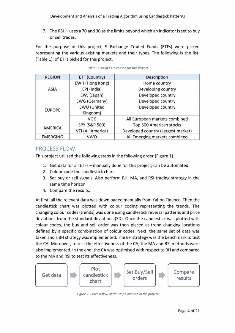
PROCESS FLOW This project utilized the following steps in the following order (Figure 1).

1. Get data for all ETFs – manually done for this project; can be automated.

2. Colour code the candlestick chart

3. Set buy or sell signals. Also perform BH, MA, and RSI trading strategy in the

same time horizon

4. Compare the results.

At first, all the relevant data was downloaded manually from Yahoo Finance. Then the

candlestick chart was plotted with colour coding representing the trends. The

changing colour codes (trends) was done using candlestick reversal patterns and price

deviations from the standard deviations (SD). Once the candlestick was plotted with

colour codes, the buy and sell order was then placed at trend changing locations

defined by a specific combination of colour codes. Next, the same set of data was

taken and a BH strategy was implemented. The BH strategy was the benchmark to test

the CA. Moreover, to test the effectiveness of the CA, the MA and RSI methods were

also implemented. In the end, the CA was optimised with respect to BH and compared

to the MA and RSI to test its effectiveness.

Figure 1: Process flow of the steps involved in the project

Get dataPlot

candlestick chart

Set Buy/Sell orders

Compare results


Page 5 of 21

GETTING DATA The data for all the ETFs were downloaded from Yahoo Finance. Data can be directly

utilized from Yahoo Finance Chart API links [3]. But for the reasons of very large number

of requests, constant internet connection, and running time for the research aspect

of this project, direct utilization of data from Chart API was not used in this project.

Instead, the data was downloaded beforehand (as a .csv file). Since the data was

downloaded from the Yahoo Finance, the data had a set time frame. Based on the

available data for each of the ETFs, an 8-year data set was found to be the largest

common data range. Hence, the data ranges from 26th July 2008 to 25th July 2016.

Assumptions 1. A 1-year time horizon consists of 252 trading days [4] (accounting for holidays).

2. An 8 x 1-year interval was chosen based on the ETFs used for this project.

3. This project used daily data for the actual trading days only.

Figure 2: Flowchart for obtaining data and finding maximum common data range

COLOUR CODING THE CANDLESTICK CHART A candlestick chart was used to plot the data obtained for each ETF. The candlestick

chart was a convenient way to display the comprehensive information about the price

of an instrument and how it moved along time. Moreover, candlesticks also have the

ability to display reversal patterns [5] that were studied by researchers. These reversal

patterns help identify moments of expected change in trends. The candlestick is

plotted using 4 points per day: open price, close price, high price and low price.

Start

Get ETF list

Get data

Find data range

For each ETF

Update Max.

data range Max. Data

Range

Stop


Page 6 of 21

The candlestick chart is colour coded to indicate the trend and performance of the

prices. The following colour codes are being used in the candlestick charting.

1. A solid fill candlestick – The closing price is higher than the opening price

2. A transparent fill candlestick – The closing price is lower than the opening price

3. Green – Up-trend

4. Red – Down-trend

5. Yellow – Sideways movement or closing price within ± (multiplier*SD)

The following (Table 2) lists the candlestick reversal patterns [5] along with all their

accepted variations were used in this project:

Table 2: Candlestick Reversal Patterns used in this project

Bearish Pattern Bullish Pattern

Hanging Man Hammer

Shooting Star Inverted Hammer

Doji (northern) Doji (southern)

Dark Cloud Cover Piercing Pattern

Bearish Engulfing Bullish Engulfing

Bearish Harami Bullish Harami

Evening Star Morning Star

Candlestick reversal patterns only indicate a potential change in trend (Green or Red

to Yellow). Another indicator was decided to indicate if we should continue with

Yellow, Green, or Red depending on the trend. For this, a recent 50-day data was used

to compute a SD. When the trend changes from Yellow to Green or Red, Green to

Green, or Red to Red, the SD is recomputed. The allowable range of price fluctuations

is the closing price of that day plus-minus a multiplier times the SD. The usage of this

SD will be mentioned in the following sections of this report.

Assumptions 1. The starting candlestick was set to Yellow colour and was the initial baseline to

judge the next candlestick.

2. A 50-day data was used to calculate the SD. 10-day, 21-day, 63-day [6] were

also used to find the best number of days to calculate the SD. In the numbers

tested, the 50-day SD gave the best results.

3. Since the volatility of each stock was different, to accommodate this

fluctuation, a multiplier was introduced to the SD to accommodate the daily

price volatility. This project puts a focus on finding the best SD multiplier for

each ETF based on a custom algorithm. This algorithm will be discussed in great

detail in the following sections.

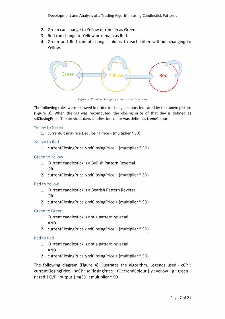
Colour coding algorithm The colour coding worked in the following way:

1. Yellow can change to Green, Red, or remain as Yellow.


Page 7 of 21

2. Green can change to Yellow or remain as Green.

3. Red can change to Yellow or remain as Red.

4. Green and Red cannot change colours to each other without changing to

Yellow.

Figure 3: Possible change of colour code directions

The following rules were followed in order to change colours indicated by the above picture

(Figure 3). When the SD was recomputed, the closing price of that day is defined as

sdClosingPrice. The previous days candlestick colour was define as trendColour.

Yellow to Green 1. currentClosingPrice ≥ sdClosingPrice + (multiplier * SD)

Yellow to Red

1. currentClosingPrice ≤ sdClosingPrice – (multiplier * SD)

Green to Yellow

1. Current candlestick is a Bullish Pattern Reversal

OR

2. currentClosingPrice ≤ sdClosingPrice – (multiplier * SD)

Red to Yellow

1. Current candlestick is a Bearish Pattern Reversal

OR

2. currentClosingPrice ≥ sdClosingPrice + (multiplier * SD)

Green to Green

1. Current candlestick is not a pattern reversal

AND

2. currentClosingPrice ≥ sdClosingPrice – (multiplier * SD)

Red to Red

1. Current candlestick is not a pattern reversal

AND

2. currentClosingPrice ≤ sdClosingPrice + (multiplier * SD)

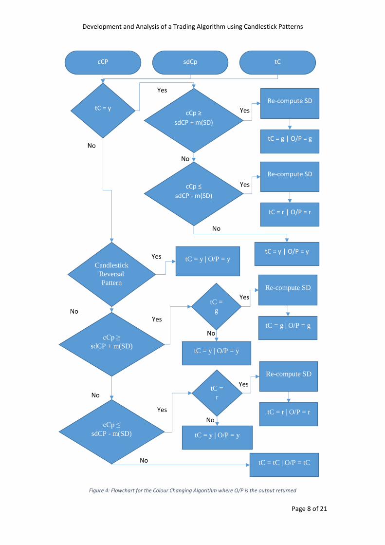
The following diagram (Figure 4) illustrates the algorithm. Legends used:- cCP :

currentClosingPrice | sdCP : sdClosingPrice | tC : trendColour | y : yellow | g : green |

r : red | O/P : output | m(SD) : multiplier * SD.

Yellow Green Red


Page 8 of 21

Figure 4: Flowchart for the Colour Changing Algorithm where O/P is the output returned

cCP sdCp tC

tC = y cCp ≥

sdCP + m(SD)

Re-compute SD

tC = g | O/P = g

cCp ≤

sdCP - m(SD)

Re-compute SD

tC = r | O/P = r

tC = y | O/P = y

Yes

No

Yes

Yes

No

No

Candlestick

Reversal

Pattern

tC = y | O/P = y

Re-compute SD

tC = g | O/P = g

Re-compute SD

tC = r | O/P = r

tC = tC | O/P = tC

Yes

Yes

No

No

tC =

g

tC =

r

tC = y | O/P = y

tC = y | O/P = y

Yes

Yes

Yes

No

No

No

cCp ≥

sdCP + m(SD)

cCp ≤

sdCP - m(SD)


Page 9 of 21

Setting the Buy and Sell order Once the candlestick chart was colour coded, the buy and sell order was set up.

Assumptions

1. The very first order has to be a buy order.

2. When a buy order was set, the entire amount-at-hand to spend was spent on

purchasing the maximum quantity of ETF at the closing price of that day.

3. When a sell order was set, the entire quantity of ETF purchased was sold at the

closing price of that day.

4. Quantities are positive integers only.

5. When a buy order has been set, the next order has to be a sell order.

Conversely, when a sell order is set, the next order has to be a buy order.

6. At a buy order, a stop- loss condition was set. For this project, the stop-loss

was at 80% of the purchase price. This merely reflects the users risk-aversion

level and the value will differ for different investors. The meaning of this was

that the price of an equity can fall 20% below its purchase price before the

stop-loss order was initiated.

The criteria that decided when to set a buy and sell order is explained in the following

points.

1. A buy order was executed when the colour code changed from Red to Yellow,

and when the previous signal was sell.

2. A sell order was executed when the colour code changed from Green to Yellow,

and when the previous signal was buy.

3. At the very beginning, if the Yellow trend changed to a Green, a buy order was

executed.

The order to buy or sell was executed as soon as the colour changed from Green/Red

to Yellow and not when the colour changed later from Yellow to Red/Green

respectively. This is because the Green/Red to Yellow indicated a pattern reversal.

Through such an indicator, the trader/investor was hoping that the pattern indeed

changed and the subsequent trend would be opposite to the trend before the pattern

reversal. A short-coming of this algorithm is when the trend does not change after the

pattern reversal is identified.

Finding the multiplier for the SD Allowing the price to move within 1 SD of the sdClosingPrice does not take into

account the historical volatility of the respective ETFs, and hence may produce

undesirable results. To account for the volatility of the respective ETFs, a range of

multipliers were used to find the multiplier that maximises the output of the program.

The range of multipliers is from 0.0 to 3.0 (both inclusive) at 0.1 intervals.

To find the SD multiplier that produces the maximum output, the Net Asset Value

(NAV) was computed for each ETF from the 8 x 1-year intervals for each SD multiplier

in the above said range. This lead to a 3-D array of size (31,8,9). 30 was for the number

of multiplier that the algorithm has to go through, 8 was the number of yearly intervals


Page 10 of 21

used in this project, and 9 was the number of ETFs used to test the algorithm. In the

pythonic language, the array is an numpy.array((31,8,9)). There were four such 3-D

arrays, one for each CA, BH, MA, and RSI.

[m1, yr1, ETF1] [m1, yr1, ETF2] … [m1, yr1, ETF9]


… … … …




… … … …


… … … …



… … … …


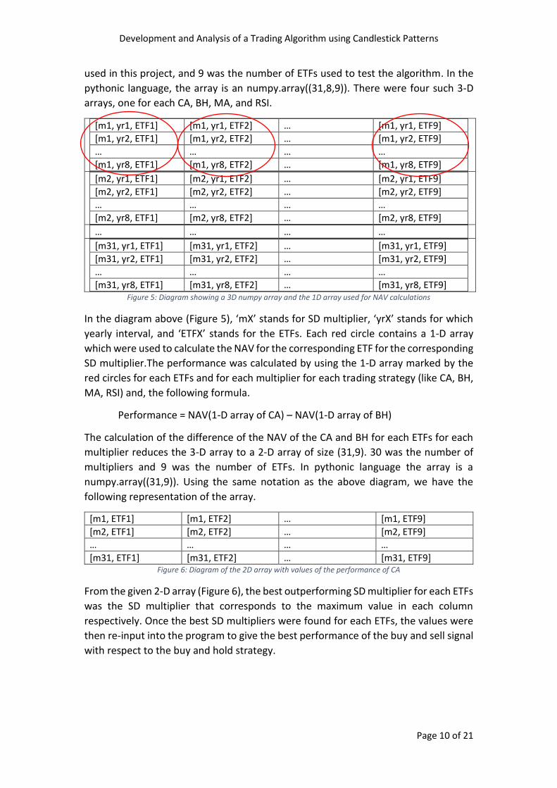
Figure 5: Diagram showing a 3D numpy array and the 1D array used for NAV calculations

In the diagram above (Figure 5), ‘mX’ stands for SD multiplier, ‘yrX’ stands for which

yearly interval, and ‘ETFX’ stands for the ETFs. Each red circle contains a 1-D array

which were used to calculate the NAV for the corresponding ETF for the corresponding

SD multiplier.The performance was calculated by using the 1-D array marked by the

red circles for each ETFs and for each multiplier for each trading strategy (like CA, BH,

MA, RSI) and, the following formula.

Performance = NAV(1-D array of CA) – NAV(1-D array of BH)

The calculation of the difference of the NAV of the CA and BH for each ETFs for each

multiplier reduces the 3-D array to a 2-D array of size (31,9). 30 was the number of

multipliers and 9 was the number of ETFs. In pythonic language the array is a

numpy.array((31,9)). Using the same notation as the above diagram, we have the

following representation of the array.

[m1, ETF1] [m1, ETF2] … [m1, ETF9]

[m2, ETF1] [m2, ETF2] … [m2, ETF9]

… … … …

[m31, ETF1] [m31, ETF2] … [m31, ETF9] Figure 6: Diagram of the 2D array with values of the performance of CA

From the given 2-D array (Figure 6), the best outperforming SD multiplier for each ETFs

was the SD multiplier that corresponds to the maximum value in each column

respectively. Once the best SD multipliers were found for each ETFs, the values were

then re-input into the program to give the best performance of the buy and sell signal

with respect to the buy and hold strategy.


Page 11 of 21

RESULTS The Custom Algorithm (CA) was optimized for the Buy & Hold (BH) strategy and then

compared with two technical trading indicators: Moving Average (MA) and Relative Strength

Index (RSI). The performance of CA in the following conclusion is relative to the performance

of BH. 100% means the performance of CA equals that of BH (there is no added advantage),

lower than 100% indicates lower performance (the investor is better off using a BH strategy),

and above 100% indicates higher performance (the investor gains using the CA strategy).

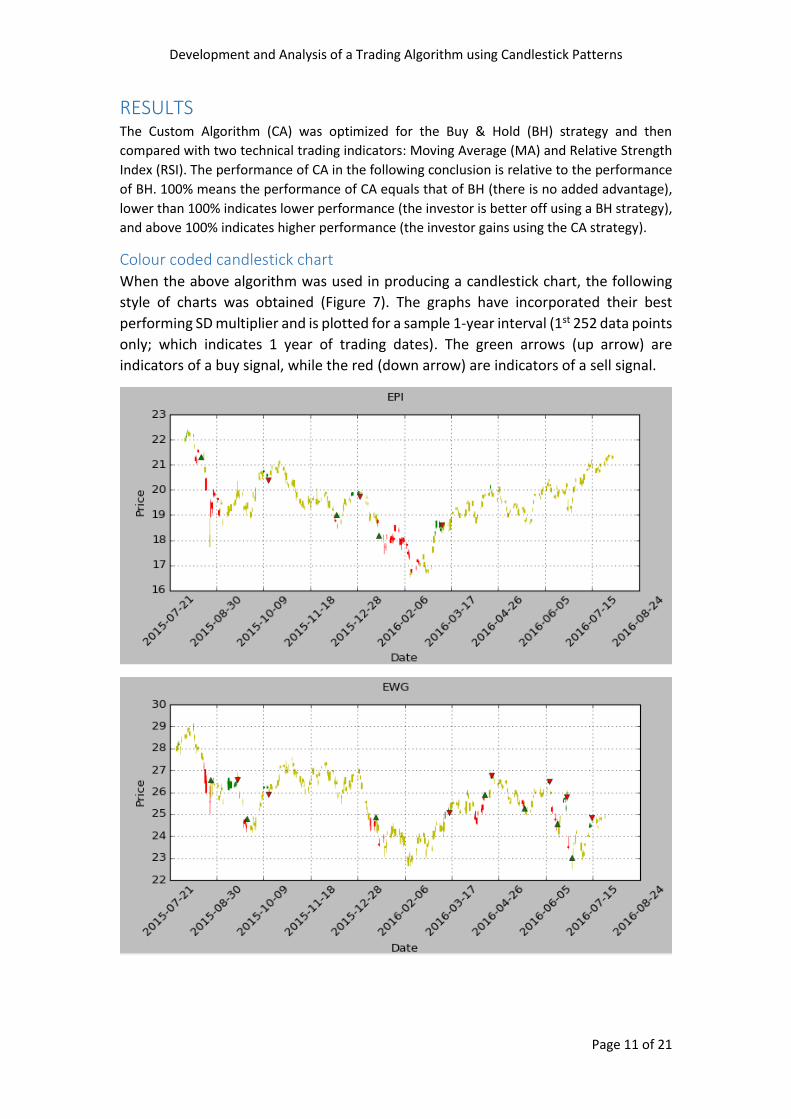
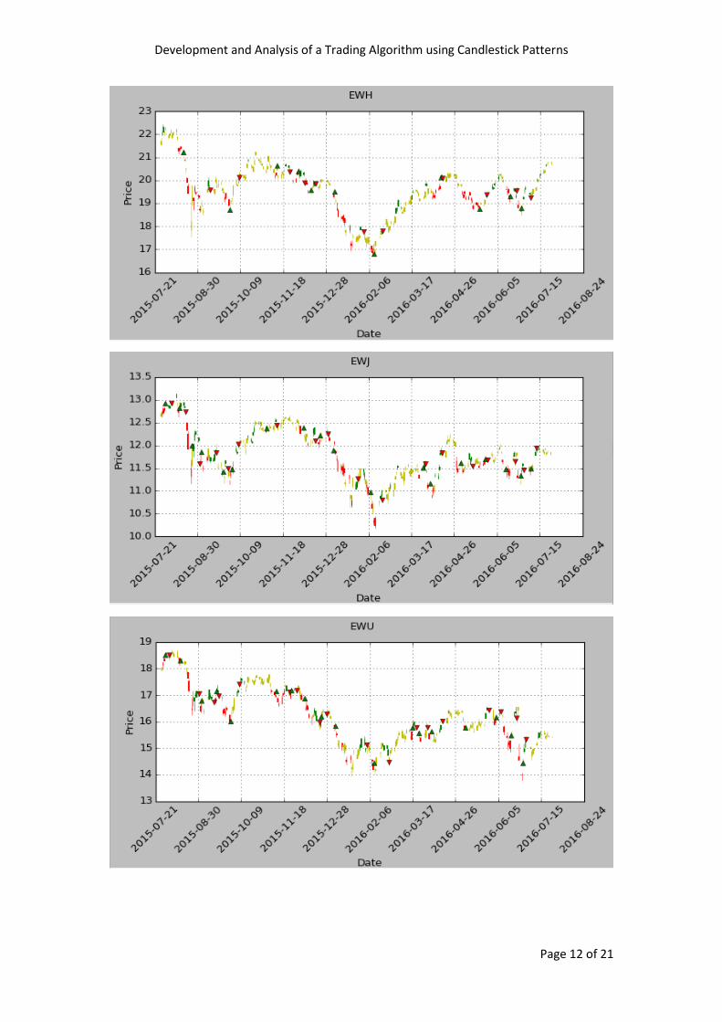
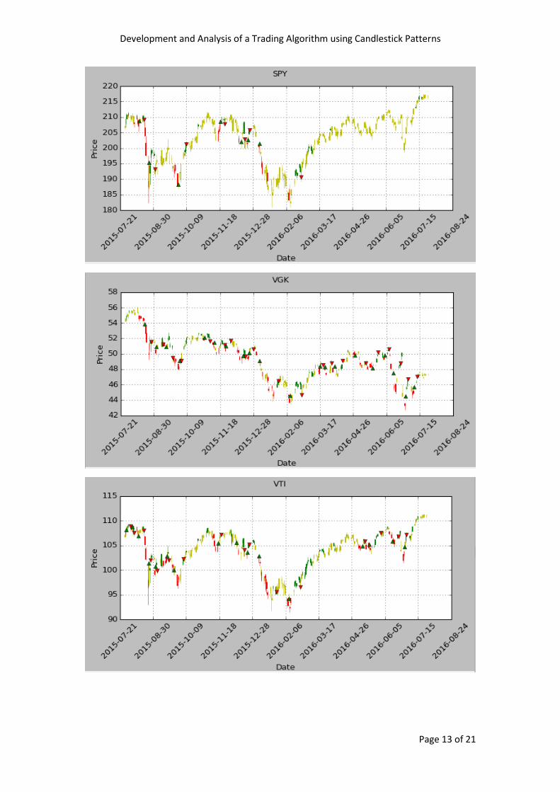
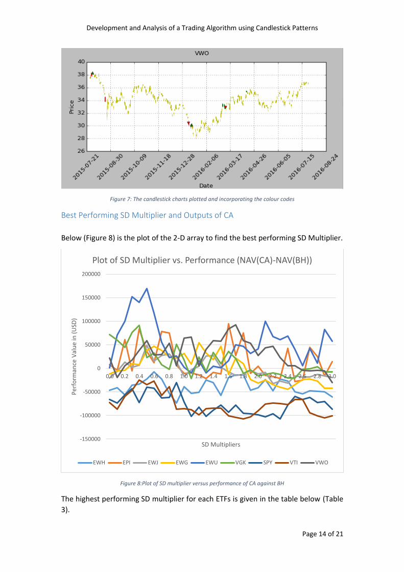
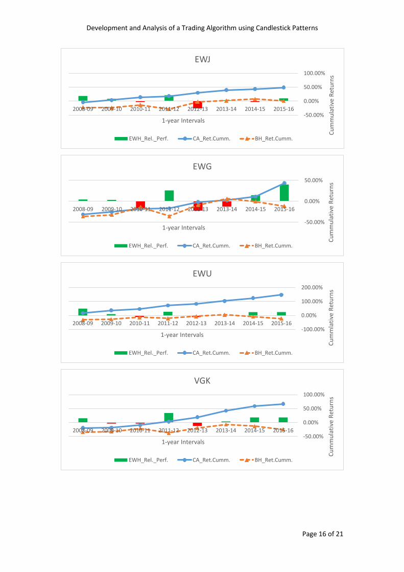
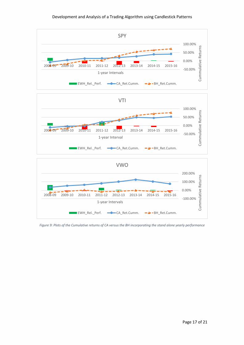
Colour coded candlestick chart When the above algorithm was used in producing a candlestick chart, the following

style of charts was obtained (Figure 7). The graphs have incorporated their best

performing SD multiplier and is plotted for a sample 1-year interval (1st 252 data points

only; which indicates 1 year of trading dates). The green arrows (up arrow) are

indicators of a buy signal, while the red (down arrow) are indicators of a sell signal.


Page 12 of 21


Page 13 of 21


Page 14 of 21

Figure 7: The candlestick charts plotted and incorporating the colour codes

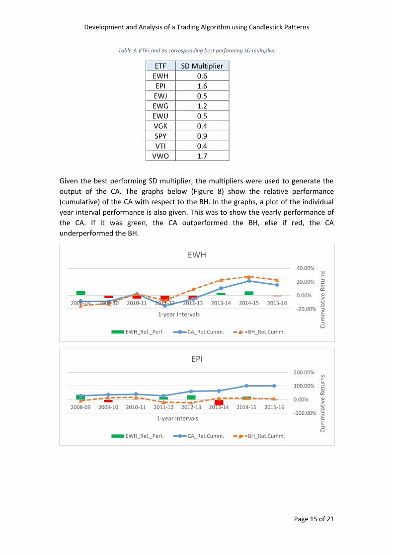
Best Performing SD Multiplier and Outputs of CA

Below (Figure 8) is the plot of the 2-D array to find the best performing SD Multiplier.

Figure 8:Plot of SD multiplier versus performance of CA against BH

The highest performing SD multiplier for each ETFs is given in the table below (Table

3).

-150000

-100000

-50000

0

50000

100000

150000

200000

0.0 0.2 0.4 0.6 0.8 1.0 1.2 1.4 1.6 1.8 2.0 2.2 2.4 2.6 2.8 3.0

Per

form

ance

Val

ue

in (

USD

)

SD Multipliers

Plot of SD Multiplier vs. Performance (NAV(CA)-NAV(BH))

EWH EPI EWJ EWG EWU VGK SPY VTI VWO


Page 15 of 21

Table 3: ETFs and its corresponding best performing SD multiplier

ETF SD Multiplier

EWH 0.6

EPI 1.6

EWJ 0.5

EWG 1.2

EWU 0.5

VGK 0.4

SPY 0.9

VTI 0.4

VWO 1.7

Given the best performing SD multiplier, the multipliers were used to generate the

output of the CA. The graphs below (Figure 8) show the relative performance

(cumulative) of the CA with respect to the BH. In the graphs, a plot of the individual

year interval performance is also given. This was to show the yearly performance of

the CA. If it was green, the CA outperformed the BH, else if red, the CA

underperformed the BH.

-20.00%

0.00%

20.00%

40.00%

2015-162014-152013-142012-132011-122010-112009-102008-09

Cu

mm

ula

tive

Ret

urn

s1-year Intervals

EWH

EWH_Rel._Perf. CA_Ret.Cumm. BH_Ret.Cumm.

-100.00%

0.00%

100.00%

200.00%

2015-162014-152013-142012-132011-122010-112009-102008-09

Cu

mm

ula

tive

Ret

urn

s

1-year Intervals

EPI



Page 16 of 21

-50.00%

0.00%

50.00%

100.00%

2015-162014-152013-142012-132011-122010-112009-102008-09

Cu

mm

ula

tive

Ret

urn

s

1-year Intervals

EWJ


-50.00%

0.00%

50.00%

2015-162014-152013-142012-132011-122010-112009-102008-09

Cu

mm

ula

tive

Ret

urn

s

1-year Intervals

EWG


-100.00%

0.00%

100.00%

200.00%

2015-162014-152013-142012-132011-122010-112009-102008-09C

um

mla

tive

Ret

urn

s1-year Intervals

EWU


-50.00%

0.00%

50.00%

100.00%

2015-162014-152013-142012-132011-122010-112009-102008-09

Cu

mm

ula

tive

Ret

urn

s

1-year Intervals

VGK



Page 17 of 21

Figure 9: Plots of the Cumulative returns of CA versus the BH incorporating the stand alone yearly performance

-50.00%

0.00%

50.00%

100.00%

2015-162014-152013-142012-132011-122010-112009-102008-09

Cu

mm

ula

tive

Ret

urn

s

1-year Intervals

SPY


-50.00%

0.00%

50.00%

100.00%

2015-162014-152013-142012-132011-122010-112009-102008-09

Cu

mm

ula

tive

Ret

urn

s

1-year Interval

VTI


-100.00%

0.00%

100.00%

200.00%

2015-162014-152013-142012-132011-122010-112009-102008-09C

um

mu

lati

ve R

etu

rns

1-year Intervals

VWO



Page 18 of 21

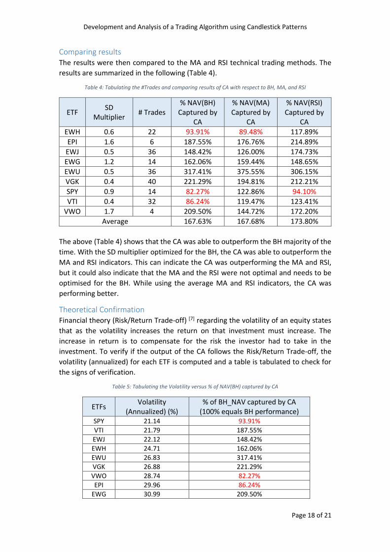
Comparing results The results were then compared to the MA and RSI technical trading methods. The

results are summarized in the following (Table 4).

Table 4: Tabulating the #Trades and comparing results of CA with respect to BH, MA, and RSI

ETF SD

Multiplier # Trades

% NAV(BH) Captured by

CA

% NAV(MA) Captured by

CA

% NAV(RSI) Captured by

CA

EWH 0.6 22 93.91% 89.48% 117.89%

EPI 1.6 6 187.55% 176.76% 214.89%

EWJ 0.5 36 148.42% 126.00% 174.73%

EWG 1.2 14 162.06% 159.44% 148.65%

EWU 0.5 36 317.41% 375.55% 306.15%

VGK 0.4 40 221.29% 194.81% 212.21%

SPY 0.9 14 82.27% 122.86% 94.10%

VTI 0.4 32 86.24% 119.47% 123.41%

VWO 1.7 4 209.50% 144.72% 172.20%

Average 167.63% 167.68% 173.80%

The above (Table 4) shows that the CA was able to outperform the BH majority of the

time. With the SD multiplier optimized for the BH, the CA was able to outperform the

MA and RSI indicators. This can indicate the CA was outperforming the MA and RSI,

but it could also indicate that the MA and the RSI were not optimal and needs to be

optimised for the BH. While using the average MA and RSI indicators, the CA was

performing better.

Theoretical Confirmation Financial theory (Risk/Return Trade-off) [7] regarding the volatility of an equity states

that as the volatility increases the return on that investment must increase. The

increase in return is to compensate for the risk the investor had to take in the

investment. To verify if the output of the CA follows the Risk/Return Trade-off, the

volatility (annualized) for each ETF is computed and a table is tabulated to check for

the signs of verification.

Table 5: Tabulating the Volatility versus % of NAV(BH) captured by CA

ETFs Volatility

(Annualized) (%) % of BH_NAV captured by CA

(100% equals BH performance) SPY 21.14 93.91%

VTI 21.79 187.55%

EWJ 22.12 148.42%

EWH 24.71 162.06%

EWU 26.83 317.41%

VGK 26.88 221.29%

VWO 28.74 82.27%

EPI 29.96 86.24%

EWG 30.99 209.50%


Page 19 of 21

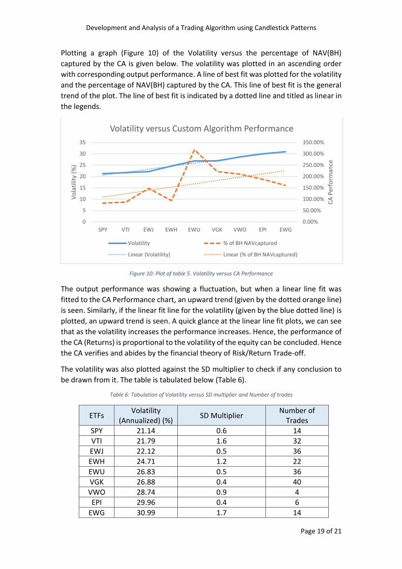
Plotting a graph (Figure 10) of the Volatility versus the percentage of NAV(BH)

captured by the CA is given below. The volatility was plotted in an ascending order

with corresponding output performance. A line of best fit was plotted for the volatility

and the percentage of NAV(BH) captured by the CA. This line of best fit is the general

trend of the plot. The line of best fit is indicated by a dotted line and titled as linear in

the legends.

Figure 10: Plot of table 5. Volatility versus CA Performance

The output performance was showing a fluctuation, but when a linear line fit was

fitted to the CA Performance chart, an upward trend (given by the dotted orange line)

is seen. Similarly, if the linear fit line for the volatility (given by the blue dotted line) is

plotted, an upward trend is seen. A quick glance at the linear line fit plots, we can see

that as the volatility increases the performance increases. Hence, the performance of

the CA (Returns) is proportional to the volatility of the equity can be concluded. Hence

the CA verifies and abides by the financial theory of Risk/Return Trade-off.

The volatility was also plotted against the SD multiplier to check if any conclusion to

be drawn from it. The table is tabulated below (Table 6).

Table 6: Tabulation of Volatility versus SD multiplier and Number of trades

ETFs Volatility

(Annualized) (%) SD Multiplier

Number of Trades

SPY 21.14 0.6 14

VTI 21.79 1.6 32

EWJ 22.12 0.5 36

EWH 24.71 1.2 22

EWU 26.83 0.5 36

VGK 26.88 0.4 40

VWO 28.74 0.9 4

EPI 29.96 0.4 6

EWG 30.99 1.7 14

0.00%

50.00%

100.00%

150.00%

200.00%

250.00%

300.00%

350.00%

0

5

10

15

20

25

30

35

SPY VTI EWJ EWH EWU VGK VWO EPI EWG

CA

Per

form

ance

Vo

lati

lity

(%)

Volatility versus Custom Algorithm Performance

Volatility % of BH NAVcaptured

Linear (Volatility) Linear (% of BH NAVcaptured)


Page 20 of 21

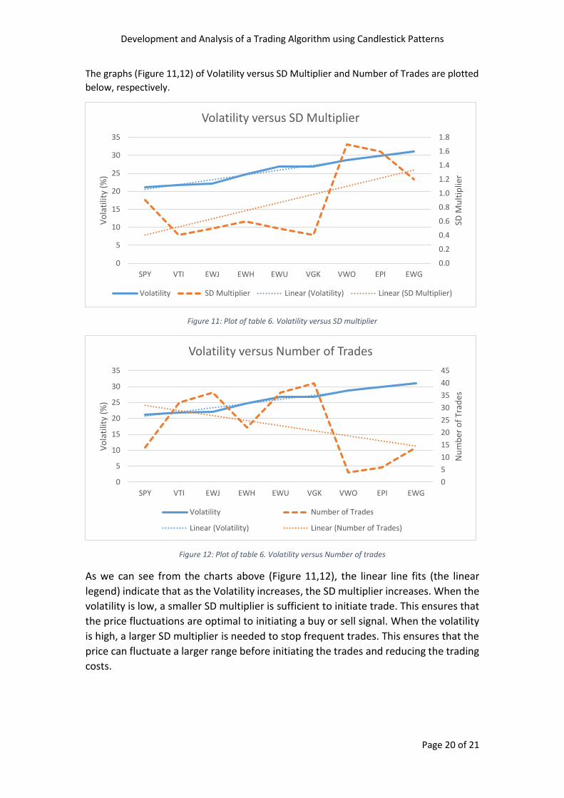
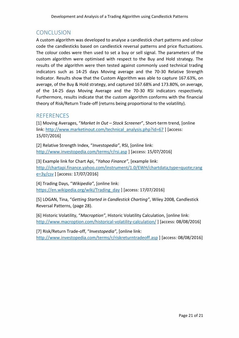
The graphs (Figure 11,12) of Volatility versus SD Multiplier and Number of Trades are plotted

below, respectively.

Figure 11: Plot of table 6. Volatility versus SD multiplier

Figure 12: Plot of table 6. Volatility versus Number of trades

As we can see from the charts above (Figure 11,12), the linear line fits (the linear

legend) indicate that as the Volatility increases, the SD multiplier increases. When the

volatility is low, a smaller SD multiplier is sufficient to initiate trade. This ensures that

the price fluctuations are optimal to initiating a buy or sell signal. When the volatility

is high, a larger SD multiplier is needed to stop frequent trades. This ensures that the

price can fluctuate a larger range before initiating the trades and reducing the trading

costs.

0.0

0.2

0.4

0.6

0.8

1.0

1.2

1.4

1.6

1.8

0

5

10

15

20

25

30

35


SD M

ult

iplie

r

Vo

lati

lity

(%)

Volatility versus SD Multiplier

Volatility SD Multiplier Linear (Volatility) Linear (SD Multiplier)

0

5

10

15

20

25

30

35

40

45

0

5

10

15

20

25

30

35


Nu

mb

er o

f Tr

ades

Vo

lati

lity

(%)

Volatility versus Number of Trades

Volatility Number of Trades

Linear (Volatility) Linear (Number of Trades)


Page 21 of 21

CONCLUSION A custom algorithm was developed to analyse a candlestick chart patterns and colour

code the candlesticks based on candlestick reversal patterns and price fluctuations.

The colour codes were then used to set a buy or sell signal. The parameters of the

custom algorithm were optimised with respect to the Buy and Hold strategy. The

results of the algorithm were then tested against commonly used technical trading

indicators such as 14-25 days Moving average and the 70-30 Relative Strength

Indicator. Results show that the Custom Algorithm was able to capture 167.63%, on

average, of the Buy & Hold strategy, and captured 167.68% and 173.80%, on average,

of the 14-25 days Moving Average and the 70-30 RSI indicators respectively.

Furthermore, results indicate that the custom algorithm conforms with the financial

theory of Risk/Return Trade-off (returns being proportional to the volatility).

REFERENCES [1] Moving Averages, “Market In Out – Stock Screener”, Short-term trend, [online

link: http://www.marketinout.com/technical_analysis.php?id=67 ] [access:

15/07/2016]

[2] Relative Strength Index, “Investopedia”, RSI, [online link:

http://www.investopedia.com/terms/r/rsi.asp ] [access: 15/07/2016]

[3] Example link for Chart Api, “Yahoo Finance”, [example link:

http://chartapi.finance.yahoo.com/instrument/1.0/EWH/chartdata;type=quote;rang

e=3y/csv ] [access: 17/07/2016]

[4] Trading Days, “Wikipedia”, [online link:

https://en.wikipedia.org/wiki/Trading_day ] [access: 17/07/2016]

[5] LOGAN, Tina, “Getting Started in Candlestick Charting”, Wiley 2008, Candlestick

Reversal Patterns, (page 28).

[6] Historic Volatility, “Macroption”, Historic Volatility Calculation, [online link:

http://www.macroption.com/historical-volatility-calculation/ ] [access: 08/08/2016]

[7] Risk/Return Trade-off, “Investopedia”, [online link:

http://www.investopedia.com/terms/r/riskreturntradeoff.asp ] [access: 08/08/2016]

http://www.marketinout.com/technical_analysis.php?id=67

http://www.investopedia.com/terms/r/rsi.asp

http://chartapi.finance.yahoo.com/instrument/1.0/EWH/chartdata;type=quote;range=3y/csv

http://chartapi.finance.yahoo.com/instrument/1.0/EWH/chartdata;type=quote;range=3y/csv

https://en.wikipedia.org/wiki/Trading_day

http://www.macroption.com/historical-volatility-calculation/

http://www.investopedia.com/terms/r/riskreturntradeoff.asp

Documents

DEVELOPMENT AND ANALYSIS OF A TRADING …rossiter/independent_studies_projects/trading... · trading indicators such ... judge the next candlestick. 2. A 50-day data was used to