Embed Size (px)
Citation preview
i
Project Report No. 364 MARCH 2005 Price: £3.85
Developing methods to improve sampling efficiency
for automated soil mapping
by
B.P. Marchant 1, R.M. Lark 1, H.C. Wheeler 2
1Biomathematics & Bioinformatics Division, Rothamsted Research,
Harpenden, Herts., AL5 2JQ 2Silsoe Research Institute, Wrest Park, Silsoe, Bedford, MK45 4HS
This is the final report of a three-year project that commenced in January 2002. The work was sponsored by the Biotechnology and Biological Sciences Research Council (BBSRC) Agri-Food committee (£142,639). As an industrial partner, HGCA provided a contract for £25,173 (project 2453). The Home-Grown Cereals Authority (HGCA) has provided funding for this project but has not conducted the research or written this report. While the authors have worked on the best information available to them, neither HGCA nor the authors shall in any event be liable for any loss, damage or injury howsoever suffered directly or indirectly in relation to the report or the research on which it is based. Reference herein to trade names and proprietary products without stating that they are protected does not imply that they may be regarded as unprotected and thus free for general use. No endorsement of named products is intended nor is it any criticism implied of other alternative, but unnamed, products.
ii
CONTENTS
Page
no.
Abstract 1
Summary 2
Chapter 1. Estimating variogram uncertainty 11
Chapter 2. Optimized sample schemes for geostatistical surveys 12
Chapter 3. Adaptive sampling for reconnaissance surveys for geostatistical mapping of the soil
18
Chapter 4. A field system for adaptive sampling 24 Acknowledgements 30 References 31
1
ABSTRACT
The goal of this project was to develop methods to sample spatial variables, such as soil or
crop properties, which are efficient and cost-effective despite the fact that we start with little
or no information about the spatial variability of the variable. Commonly when we begin a
survey we do not know in advance how intensively to sample, and so we run the risk of
completing then survey then finding that we have substantially over-sampled and so wasted
effort, or that we are not able to produce a reasonable map from the our data because they are
too sparse.
We developed an approach to optimization of sampling for a single-phase geostatistical
survey, showing how the combined uncertainty of our model of spatial variation (variogram),
and predictions under spatial variation could be quantified and minimized, assuming some
prior distribution of variogram parameters. We showed, using simulation, how this scheme
successfully models prediction error variance, and how under different underlying kinds of
spatial variation the resulting sample schemes achieve the dual goal of allowing adequate
estimates of the variogram and disposing sample points from which to map the variable.
We then developed a fully adaptive sample scheme. Under this the sampling is divided into
phases. In the initial phases (reconnaissance) our uncertainty about the required final sample
intensity is reduced by sampling designed to yield maximum information, and at the end of
each phase we are presented with a representation of this uncertainty which allows us to
decide whether further reconnaissance sampling is justified or whether we should proceed to a
final sampling phase before mapping. This final phase may be designed so as to allow for the
existing observations, and so to save on total sampling effort. We demonstrated the value of
this method by simulation.
We built a field system to implement these algorithms for mapping the water content of the
soil with a sensor. This uses GPS to record locations, and to guide the user to selected sample
sites. We applied the system in a survey of a field, and showed how it identified the relatively
sparse sample effort needed to map the variable to a specified precision.
In conclusion, we have shown how substantial efficiencies in sampling are possible using
appropriate algorithms. Some of the methods we have used, notably the spatial simulated
annealing algorithm to select sample points, could be applied to simpler sampling problems
that farmers and agronomists face.
2
SUMMARY
Background: the problem
Spatial variability of soil and other variables at within-field scales is recognized as both a
challenge and an opportunity for farmers and their advisers (see, for example, the HGCA
Research Strategy, 2004). It is also recognized that one of the biggest problems for
management of within-field variation is obtaining adequate information on the variations of
important variables at acceptable cost.
These issues have been tackled in previous projects funded by the HGCA. Lark et al. (1998,
2003) considered, among other problems, how ancillary variables, notably yield data, might
be used to direct sampling more efficiently. One of their principal conclusions, based on a
large set of fields across the arable landscape of Great Britain, was that
while all fields are variable, some fields are more variable than others.
This gnomic statement has significant implications. Most importantly it means that we
cannot, with confidence, present farmers or agronomists with a sampling strategy that will be
efficient in all fields. This conclusion is supported by the work of Oliver and Frogbrook
(2004) who showed that, if soil properties are to be mapped with adequate precision, then the
effort needed will differ between fields. Their results suggested that the standard practice of
sampling on a 100-m grid was unlikely to resolve spatial variation adequately.
The farmer or agronomist is left in a quandary. It may be summarized thus:
I am told that sampling every 100m is unlikely to generate adequate
information for spatially variable management, but I am not given an
alternative intensity against which I can make judgements about the costs
and benefits of this information. On the basis of what we are told a 50-m
sample interval (four times more costly than the standard) might turn out to
be woefully inadequate in some fields and wastefully generous in others.
How, then, am I to decide?
The research cited above provides some answers. Lark et al. (2003) presented an algorithm to
make a prediction in absolute terms as to whether the scales and magnitudes of variation
within a field are likely to justify attempts at precision management. They also showed how
3
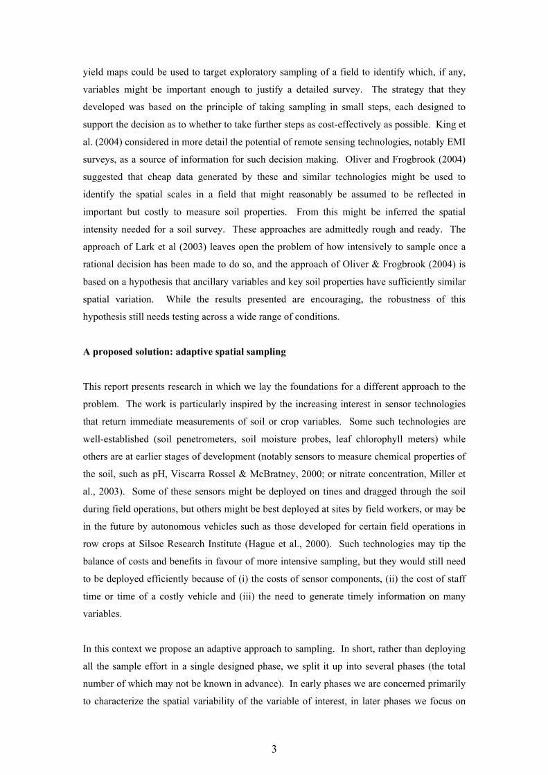
yield maps could be used to target exploratory sampling of a field to identify which, if any,
variables might be important enough to justify a detailed survey. The strategy that they
developed was based on the principle of taking sampling in small steps, each designed to
support the decision as to whether to take further steps as cost-effectively as possible. King et
al. (2004) considered in more detail the potential of remote sensing technologies, notably EMI
surveys, as a source of information for such decision making. Oliver and Frogbrook (2004)
suggested that cheap data generated by these and similar technologies might be used to
identify the spatial scales in a field that might reasonably be assumed to be reflected in
important but costly to measure soil properties. From this might be inferred the spatial
intensity needed for a soil survey. These approaches are admittedly rough and ready. The
approach of Lark et al (2003) leaves open the problem of how intensively to sample once a
rational decision has been made to do so, and the approach of Oliver & Frogbrook (2004) is
based on a hypothesis that ancillary variables and key soil properties have sufficiently similar
spatial variation. While the results presented are encouraging, the robustness of this
hypothesis still needs testing across a wide range of conditions.
A proposed solution: adaptive spatial sampling
This report presents research in which we lay the foundations for a different approach to the
problem. The work is particularly inspired by the increasing interest in sensor technologies
that return immediate measurements of soil or crop variables. Some such technologies are
well-established (soil penetrometers, soil moisture probes, leaf chlorophyll meters) while
others are at earlier stages of development (notably sensors to measure chemical properties of
the soil, such as pH, Viscarra Rossel & McBratney, 2000; or nitrate concentration, Miller et
al., 2003). Some of these sensors might be deployed on tines and dragged through the soil
during field operations, but others might be best deployed at sites by field workers, or may be
in the future by autonomous vehicles such as those developed for certain field operations in
row crops at Silsoe Research Institute (Hague et al., 2000). Such technologies may tip the
balance of costs and benefits in favour of more intensive sampling, but they would still need
to be deployed efficiently because of (i) the costs of sensor components, (ii) the cost of staff
time or time of a costly vehicle and (iii) the need to generate timely information on many
variables.
In this context we propose an adaptive approach to sampling. In short, rather than deploying
all the sample effort in a single designed phase, we split it up into several phases (the total
number of which may not be known in advance). In early phases we are concerned primarily
to characterize the spatial variability of the variable of interest, in later phases we focus on
4
sampling to support mapping of the variable by geostatistical interpolation. Any phase is
designed using information from past phases (including the known values of the property at
previously-sampled sites) and generates information used to decide how to sample next. We
hypothesize that, by such adaptive sampling, it should be possible to arrive at an efficient
final sampling scheme in the absence of any prior information on variability. However,
information from ancillary sources, such as those proposed by Oliver & Frogbrook (2004)
could be used to initiate the process, although if it turns out that the ancillary data is a poor
guide in any specific case this will be recognized.
The proposed approach draws on various geostatistical studies. The earliest is that by
McBratney et al. (1981) who showed how, given a variogram function that describes the
spatial variability of a property, we may plan a sampling scheme to ensure that the property is
mapped to some specified precision. This left open the problem of how to specify the
variogram, given that this must be based on data, and how we should allow for uncertainty in
the variogram estimates since these result in uncertainty both in the sample design and the
estimates generated after sampling. We tackle these problems in this project. Another
important precursor to our work is the study by Van Groenigen (1999). This showed how an
optimization method, simulated annealing, can be used to generate a spatial sampling array
that minimizes some objective function (such as the maximum expected error variance of a
geostatistical prediction at any site in a field). Lark (2002) applied this to the problem of
variogram estimation, showing how the best sample design for this purpose depends on the
underlying variogram itself, and demonstrating the principle of adaptive approaches in a two-
phase scheme where an estimate of the variogram from an initial sample on transects is used
to choose the disposition of a further set of points to refine this estimate.
This sets the context for the work that we present here. We tackle the following questions.
1. How can the uncertainty attendant on an estimated variogram model be
described quantitatively? This is necessary for our purpose if we are to allow for
the uncertainty of variograms estimated in early phases of sampling when designing
further phases. As is indicated in Chapter 1 (an abstract of a published paper), there
are problems with the methods that have previously been proposed for this, and we
tested and evaluated these as a necessary preamble to subsequent steps.
2. Can we design sampling schemes for geostatistical mapping in which the overall
uncertainty of predictions, due both to spatial variation and uncertainty in our
variogram, are known and minimized? In this way we deal with the limitation in

5
the approach of McBratney et al (1981) that the variogram is assumed known.
However, the problem is a complex one since the uncertainty of a variogram,
estimated from a particular sample scheme, depends on the (unknown) variogram
itself. We address these problems in Chapter 2.
3. How can the uncertainty about the specifications of a final sample grid, given a
set of observations and their experimental variogram, be quantified, and can this
be built into an adaptive sampling scheme for any variable of unknown
variability? These problems are addressed in Chapter 3 of this report.
4. Can these schemes be incorporated into a working field system? In Chapter 4 we
describe briefly a field system, and illustrate its use in a reconnaissance survey to
identify a sampling scheme for mapping soil water content.
Towards adaptive sampling: what we have done
1. How can the uncertainty attendant on an estimated variogram model be
described quantitatively?
We concluded that existing expressions for the uncertainty of variogram parameter
estimates, which were largely untested before this study, could give misleading
predictions of the error in non-linear parameters: i.e. the distance parameters which
control the distance over which a variable shows spatial dependence. Since this has
significant implications for problems like design of a survey grid, this put limitations
on how far we could use these expressions in further work, as well as being an
important finding for geostatistics in its own right. We used a Bayesian formulation
of variogram uncertainty for further work.
2. Can we design sampling schemes for geostatistical mapping in which the overall
uncertainty of predictions, due both to spatial variation and uncertainty in our
variogram, are known and minimized?
In this part of the project we addressed the problem of how to optimize a sampling
scheme in one phase to support both estimation of the variogram and subsequent
kriging. The critical issue here was to allow for how error in the specified variogram
will propagate through to error in the kriging estimates. We derived an expression for
the combined effects of spatial variation, and error in our model of this (variogram)
on the error variance of kriged predictions, and tested these by simulations. Using
spatial simulated annealing (Van Groenigen, 1999) it was then possible to design
6
overall sampling schemes, given the variogram. It was clear how these automatically
balanced the division of effort between variogram estimation and the more spatially
regular sampling aimed primarily at ensuring that no site is too far from its nearest
neighbouring points for prediction. Since in practice we do not know the variogram
at the start of this procedure we proposed a Bayesian framework in which we design
the sampling scheme to minimize an error variance over a set of plausible
variograms. This offers a framework within which ancillary data or knowledge of
variation of the same property in similar conditions could be used to aid sample
design.
3. How can the uncertainty about the specifications of a final sample grid, given a
set of observations and their experimental variogram, be quantified, and can this
be built into an adaptive sampling scheme for any variable of unknown
variability?
Here we developed a fully adaptive sampling scheme. At the end of each phase of
sampling we can compute, in a Bayesian framework, a probability distribution for the
interval of a sample grid which will allow us to map the variable of interest to a
specified precision. We may then consider the number of additional samples that are
needed to complete a survey for geostatistical mapping, such that the target precision
is met or exceeded with some probability. We may select a suitably conservative
confidence level (e.g. 95%) and compare the number with what we would need if the
best estimate of the variogram from our existing data were correct. On the basis of
this we can decide whether it is worth collecting further data in the hope that we can
then confidently proceed to map from a smaller sample, or whether further reductions
in uncertainty about the variogram are likely to be significant. If further samples are
to be selected for variogram estimation then the spatial simulated annealing method is
used to select the most informative locations to sample.
We are also able to plan the final survey allowing for the fact that the field of interest
is already sampled at many sites, so that an entirely regular grid is not needed in order
to achieve a target maximum variance of the estimation error. We demonstrated the
utility of these methods in simulation studies.
4. Can these schemes be incorporated into a working field system?
All the work reported above is statistical research, supported by simulation studies.
However, we also wished to show that the approach was feasible in practice. To this
end a field system was built. The key components are a Tablet PC which can run the

7
algorithms, an RTK GPS system for determining position, the antenna of which is
mounted on a staff bearing a Delta-T theta probe that measures soil water content.
The probe and the GPS are both connected to the PC so measurements and positions
can be recorded. The PC also runs an algorithm to direct the user to a sample site
selected by one of the methods described above.
Once the system was designed and built we used it in a reconnaissance survey of soil
water content in a field as described under (3) above. We specified a target error
variance for predictions before the survey, and a total of 75 points were sampled in
four phases before it was decided that the uncertainty in the final sample grid could
not be reduced further. The final survey could be completed either by adding 15
more points in a regular grid edited to remove redundant points, or by adding 4 more
points selected by spatial simulated annealing. We noted that the target error
variance was relatively large, and that it would have been easy to over-sample this
field without the adaptive approach in force.
The figure below shows the field system in action. The results of this trial survey are
shown in the full report.
Figure 0.1. The field system for adaptive sampling for geostatistical mapping of soil
water content.

8
Implications
As we have noted this project was funded primarily by the BBSRC as a piece of research into
the basic science of spatial sampling. It was thought to be of strategic relevance to HGCA,
rather than generating immediate solutions to Levy-payers' problems. We would suggest that
the strategic implications of this work are as follows.
1. We have shown that there is scope to make the sampling of spatial variables less hit-
and-miss through the methods that we have developed. The adaptive sampling
scheme ensures that, even when we have no prior knowledge about the variability of
a property, we end up with a sampling scheme that reflects the spatial scales at which
it varies. This can be done without any prior knowledge, although efficiencies may
be achieved if we do have some prior information.
2. This approach is most suited to systems where soil properties can be measured in situ,
and with increasing interest in development of sensor systems for soil and crop
properties this work positions the industry to ensure that such sensors are deployed
most efficiently.
3. Despite (2), it is also possible that we could apply these methods to other variables
where the cost of soil analysis is large, and the soil property is stable so that delays in
time between the phases do not create problems. For example, Oliver & Frogbrook
(2004) suggested that some variables, which are stable, might be measured in a single
survey which would yield information of long-term value to the farmer. This might
be information on physical properties of the soil, such as particle size distribution.
These could be mapped adaptively in a number of phases, and given the costs of
laboratory determination this might be worthwhile.
4. There is scope to use some of the spatial methods used and developed in this project
to study simpler sampling problems in agriculture. We have not discussed this in
detail in the main report, since it was not part of the original project proposal.
However, the spatial simulated annealing scheme was used to consider how best to
form a bulk (composite) sample from which to estimate the mean value of a property
in a single field. We specified an average variogram for phosphorous concentration
in topsoils of agricultural fields in the Netherlands, as presented by Brus et al (1999).
Using this we found a sample design for eight points to sample a square field (right-
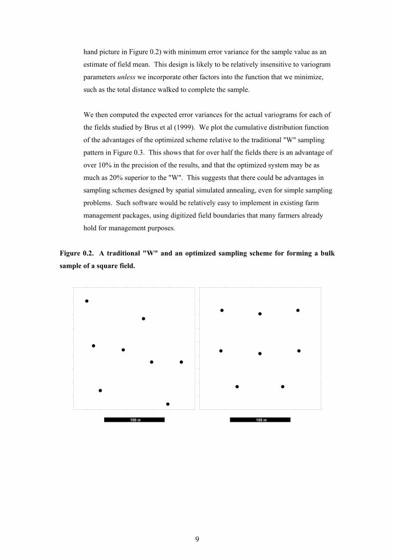
9
hand picture in Figure 0.2) with minimum error variance for the sample value as an
estimate of field mean. This design is likely to be relatively insensitive to variogram
parameters unless we incorporate other factors into the function that we minimize,
such as the total distance walked to complete the sample.
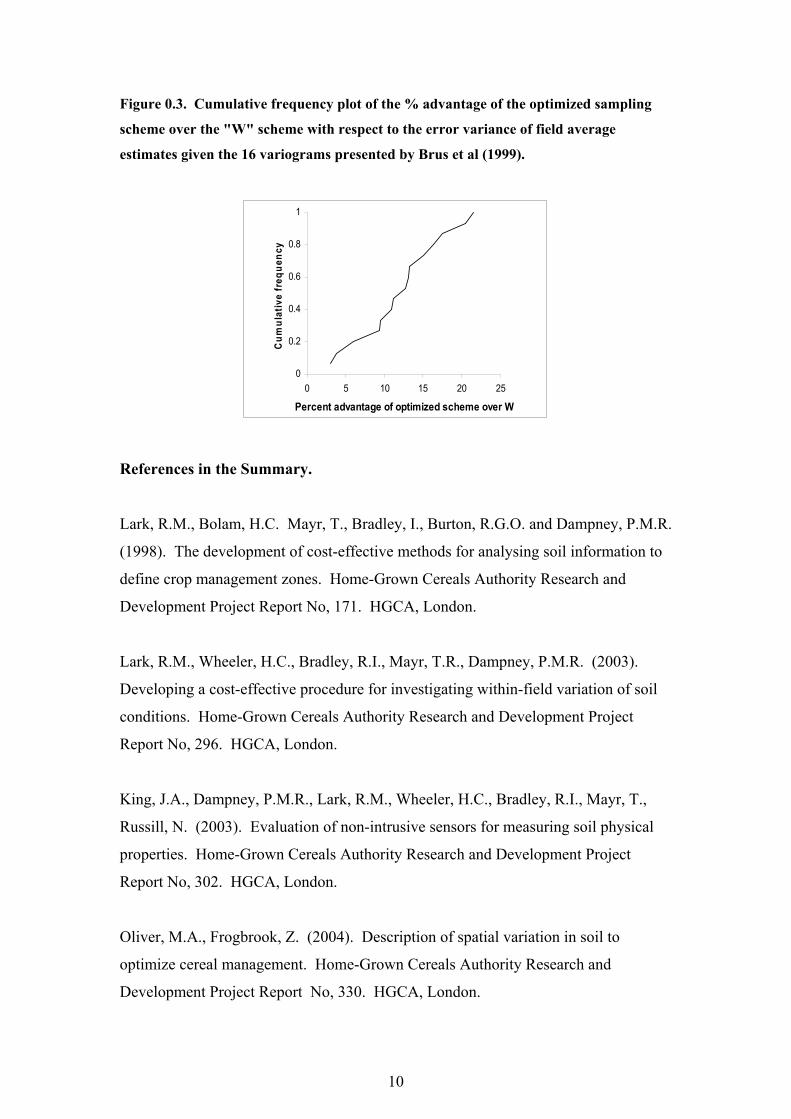
We then computed the expected error variances for the actual variograms for each of
the fields studied by Brus et al (1999). We plot the cumulative distribution function
of the advantages of the optimized scheme relative to the traditional "W" sampling
pattern in Figure 0.3. This shows that for over half the fields there is an advantage of
over 10% in the precision of the results, and that the optimized system may be as
much as 20% superior to the "W". This suggests that there could be advantages in
sampling schemes designed by spatial simulated annealing, even for simple sampling
problems. Such software would be relatively easy to implement in existing farm
management packages, using digitized field boundaries that many farmers already
hold for management purposes.
Figure 0.2. A traditional "W" and an optimized sampling scheme for forming a bulk
sample of a square field.
100 m 100 m
10
Figure 0.3. Cumulative frequency plot of the % advantage of the optimized sampling
scheme over the "W" scheme with respect to the error variance of field average
estimates given the 16 variograms presented by Brus et al (1999).
0
0.2
0.4
0.6
0.8
1
0 5 10 15 20 25
Percent advantage of optimized scheme over W
Cum
ulat
ive
freq
uenc
y
References in the Summary.
Lark, R.M., Bolam, H.C. Mayr, T., Bradley, I., Burton, R.G.O. and Dampney, P.M.R.
(1998). The development of cost-effective methods for analysing soil information to
define crop management zones. Home-Grown Cereals Authority Research and
Development Project Report No, 171. HGCA, London.
Lark, R.M., Wheeler, H.C., Bradley, R.I., Mayr, T.R., Dampney, P.M.R. (2003).
Developing a cost-effective procedure for investigating within-field variation of soil
conditions. Home-Grown Cereals Authority Research and Development Project
Report No, 296. HGCA, London.
King, J.A., Dampney, P.M.R., Lark, R.M., Wheeler, H.C., Bradley, R.I., Mayr, T.,
Russill, N. (2003). Evaluation of non-intrusive sensors for measuring soil physical
properties. Home-Grown Cereals Authority Research and Development Project
Report No, 302. HGCA, London.
Oliver, M.A., Frogbrook, Z. (2004). Description of spatial variation in soil to
optimize cereal management. Home-Grown Cereals Authority Research and
Development Project Report No, 330. HGCA, London.
11
CHAPTER 1. ESTIMATING VARIOGRAM UNCERTAINTY
We do not report this work in any detail here. Information may be found in the following
paper, and we include the abstract.
Marchant, B. P. & Lark, R.M. (2004). Estimating variogram uncertainty. Mathematical
Geology, vol 36, no. 8 pp. 867–898.
Abstract
The variogram is central to any geostatistical survey, but the precision of a variogram
estimated from sample data by the method of moments is unknown. In previous studies
theoretical expressions have been derived in order to approximate uncertainty in both
estimates of the experimental variogram and fitted variogram models. These expressions rely
upon various statistical assumptions about the data and are largely untested. They express
variogram uncertainty as functions of the sampling positions and the ergodic variogram.
Extensive simulation tests show that for a Gaussian variable with a known isotropic
variogram, the uncertainty of the experimental variogram estimate may be accurately
determined via these theoretical expressions. In practice however, the variogram of the
variable is unknown and the fitted variogram model must instead be used. For sampling
schemes of 100 points or more, this is seen to have only a small effect on the accuracy of the
uncertainty estimate.
The theoretical expressions generally overestimate the precision of fitted variogram
parameters. The uncertainty of the fitted parameters are seen to be more accurately
determined by simulating multiple experimental variograms and fitting variogram models to
these.
The tests emphasise the importance of distinguishing between the ergodic and non-ergodic
variogram. Most studies discussing variogram uncertainty describe the uncertainty associated
with estimates to the ergodic variogram. Generally however, it is the non-ergodic variogram
which is of interest. For dense sampling schemes, estimates of the non-ergodic variogram are
shown to be significantly more precise than estimates of the ergodic variogram. It is
important, when designing efficient sampling schemes or fitting variogram models, that the
appropriate expression for variogram uncertainty is applied.
12
CHAPTER 2. OPTIMIZED SAMPLE SCHEMES FOR GEOSTATISTICAL
SURVEYS
Introduction
The uncertainty associated with a soil map estimated by ordinary kriging is commonly
approximated by the kriging variance. The kriging variance depends upon the sample scheme
from which the soil map is estimated and the variogram of the variable being mapped. If the
variogram is known exactly then the kriging variance may be calculated prior to sampling.
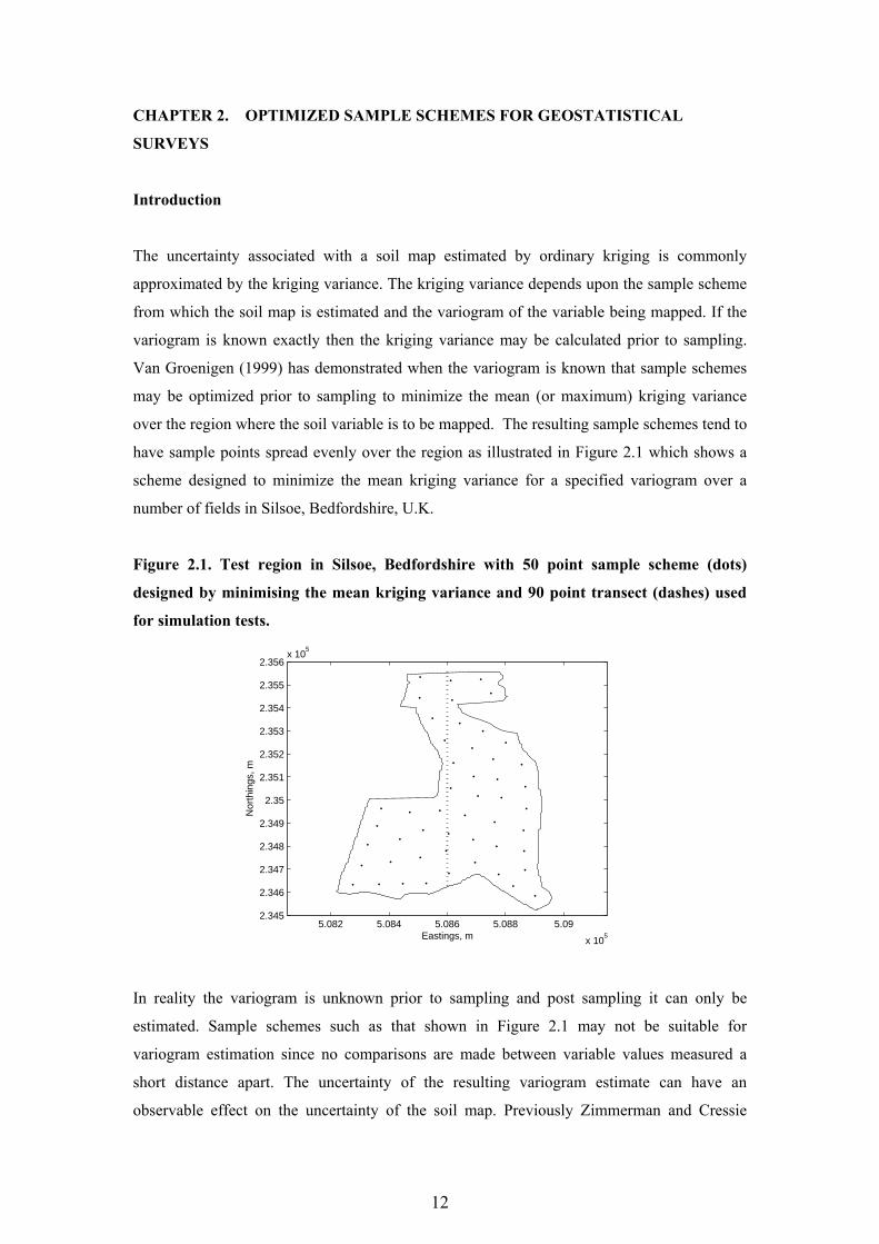
Van Groenigen (1999) has demonstrated when the variogram is known that sample schemes
may be optimized prior to sampling to minimize the mean (or maximum) kriging variance
over the region where the soil variable is to be mapped. The resulting sample schemes tend to
have sample points spread evenly over the region as illustrated in Figure 2.1 which shows a
scheme designed to minimize the mean kriging variance for a specified variogram over a
number of fields in Silsoe, Bedfordshire, U.K.
Figure 2.1. Test region in Silsoe, Bedfordshire with 50 point sample scheme (dots)
designed by minimising the mean kriging variance and 90 point transect (dashes) used
for simulation tests.
5.082 5.084 5.086 5.088 5.09
x 105
2.345
2.346
2.347
2.348
2.349
2.35
2.351
2.352
2.353
2.354
2.355
2.356x 10
5
Eastings, m
Nor
thin
gs, m
In reality the variogram is unknown prior to sampling and post sampling it can only be
estimated. Sample schemes such as that shown in Figure 2.1 may not be suitable for
variogram estimation since no comparisons are made between variable values measured a
short distance apart. The uncertainty of the resulting variogram estimate can have an
observable effect on the uncertainty of the soil map. Previously Zimmerman and Cressie
13
(1992) showed that the component of uncertainty in a soil map due to variogram uncertainty
may be approximated once the sampled data have been collected. We wish to approximate
this component of uncertainty prior to sampling in order to design sample schemes for which
the total uncertainty is minimized.
Approximation of the propagation of variogram uncertainty into kriging
In the previous chapter we discussed how the uncertainty in the estimation of a variogram
from sampled data may be approximated. Generally, variogram uncertainty is of little interest
in itself; the key concern is how this uncertainty propagates into soil maps. We have extended
work by Zimmerman and Cressie (1992) to derive an expression for the component of error in
soil maps generated by ordinary kriging due to variogram uncertainty. The size of this
component of uncertainty depends upon the sample scheme employed and the variogram of
the variable but not directly upon the sampled data. Thus if a particular variogram is assumed
both the kriging variance and the uncertainty in the soil map due to variogram uncertainty
may be calculated prior to sampling. The sum of these quantities is an approximation to the
total error in a soil map estimate which we denote 2Tσ .
In this study we focus upon variograms defined by a spherical model:
−+=
3
10 21
23)(
ah
ahcchγ for ,0 ah ≤<
10)( cch +=γ for ,ah >
.0)0( =γ
Here )(hγ denotes the variogram for lag distance h , 0c denotes the nugget effect, 1c denotes
the sill and a denotes the range of spatial correlation.
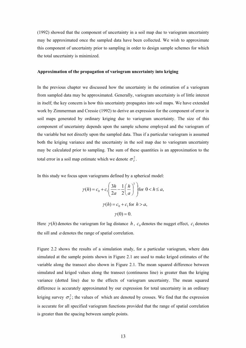
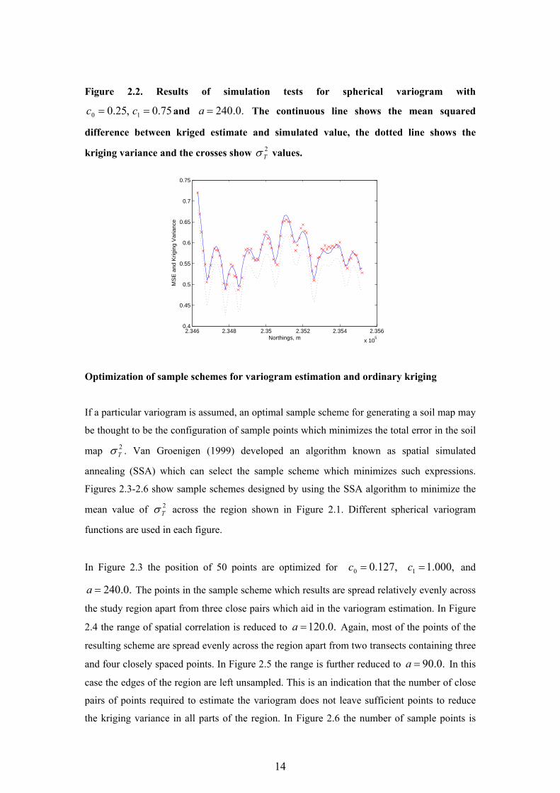
Figure 2.2 shows the results of a simulation study, for a particular variogram, where data
simulated at the sample points shown in Figure 2.1 are used to make kriged estimates of the
variable along the transect also shown in Figure 2.1. The mean squared difference between
simulated and kriged values along the transect (continuous line) is greater than the kriging
variance (dotted line) due to the effects of variogram uncertainty. The mean squared
difference is accurately approximated by our expression for total uncertainty in an ordinary
kriging survey 2Tσ ; the values of which are denoted by crosses. We find that the expression
is accurate for all specified variogram functions provided that the range of spatial correlation
is greater than the spacing between sample points.
14
Figure 2.2. Results of simulation tests for spherical variogram with
,25.00 =c 75.01 =c and .0.240=a The continuous line shows the mean squared
difference between kriged estimate and simulated value, the dotted line shows the
kriging variance and the crosses show 2Tσ values.
2.346 2.348 2.35 2.352 2.354 2.356
x 105
0.4
0.45
0.5
0.55
0.6
0.65
0.7
0.75
Northings, m
MS
E a
nd K
rigin
g V
aria
nce
Optimization of sample schemes for variogram estimation and ordinary kriging
If a particular variogram is assumed, an optimal sample scheme for generating a soil map may
be thought to be the configuration of sample points which minimizes the total error in the soil
map 2Tσ . Van Groenigen (1999) developed an algorithm known as spatial simulated
annealing (SSA) which can select the sample scheme which minimizes such expressions.
Figures 2.3-2.6 show sample schemes designed by using the SSA algorithm to minimize the
mean value of 2Tσ across the region shown in Figure 2.1. Different spherical variogram
functions are used in each figure.
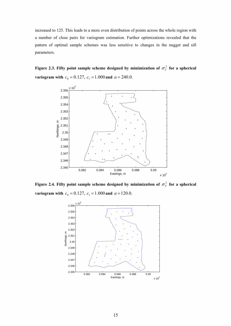
In Figure 2.3 the position of 50 points are optimized for ,127.00 =c ,000.11 =c and
.0.240=a The points in the sample scheme which results are spread relatively evenly across
the study region apart from three close pairs which aid in the variogram estimation. In Figure
2.4 the range of spatial correlation is reduced to .0.120=a Again, most of the points of the
resulting scheme are spread evenly across the region apart from two transects containing three
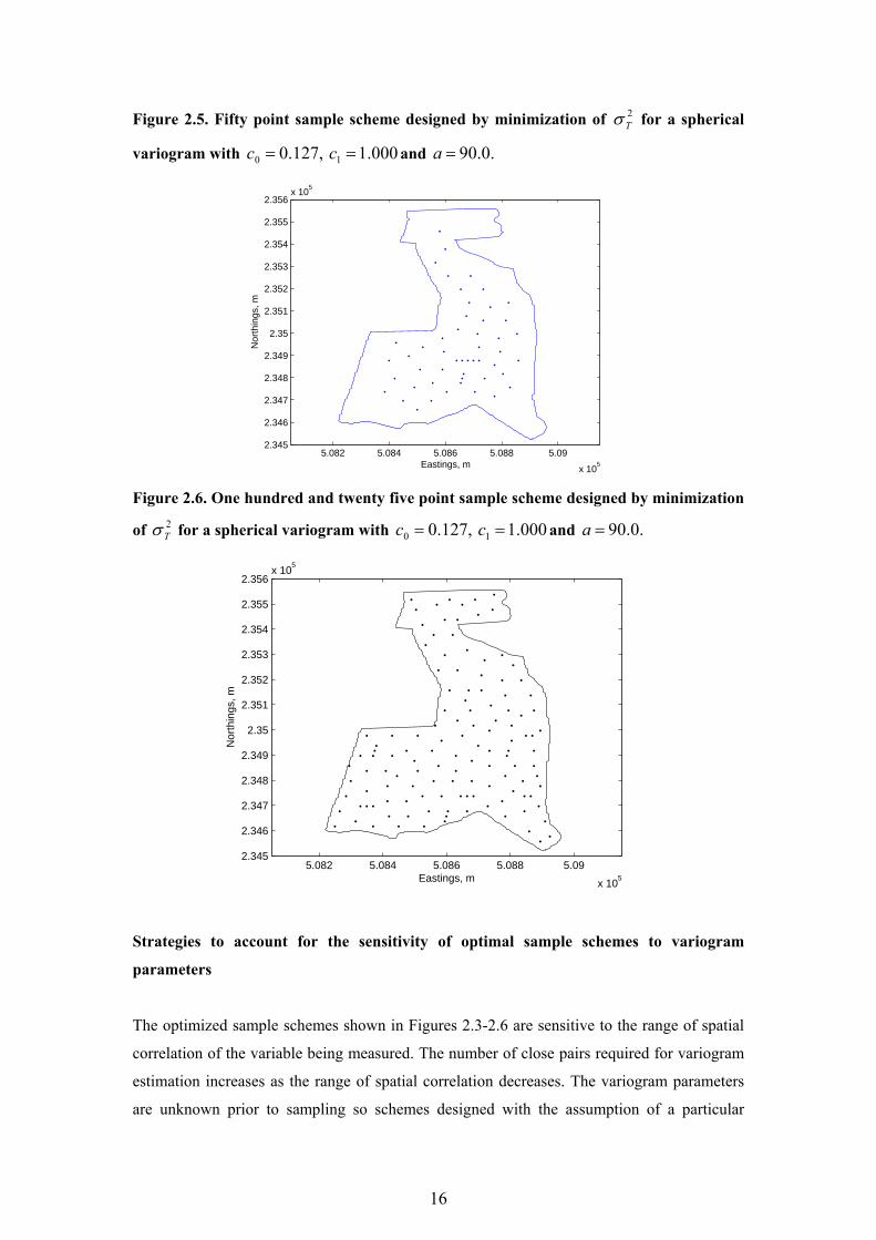
and four closely spaced points. In Figure 2.5 the range is further reduced to .0.90=a In this
case the edges of the region are left unsampled. This is an indication that the number of close
pairs of points required to estimate the variogram does not leave sufficient points to reduce
the kriging variance in all parts of the region. In Figure 2.6 the number of sample points is
15
increased to 125. This leads to a more even distribution of points across the whole region with
a number of close pairs for variogram estimation. Further optimizations revealed that the
pattern of optimal sample schemes was less sensitive to changes in the nugget and sill
parameters.
Figure 2.3. Fifty point sample scheme designed by minimization of 2Tσ for a spherical
variogram with ,127.00 =c 000.11 =c and .0.240=a
5.082 5.084 5.086 5.088 5.09
x 105
2.345
2.346
2.347
2.348
2.349
2.35
2.351
2.352
2.353
2.354
2.355
2.356x 10
5
Nor
thin
gs, m
Eastings, m
Figure 2.4. Fifty point sample scheme designed by minimization of 2Tσ for a spherical
variogram with ,127.00 =c 000.11 =c and .0.120=a
5.082 5.084 5.086 5.088 5.09
x 105
2.345
2.346
2.347
2.348
2.349
2.35
2.351
2.352
2.353
2.354
2.355
2.356x 10
5
Eastings, m
Nor
thin
gs, m
16
Figure 2.5. Fifty point sample scheme designed by minimization of 2Tσ for a spherical
variogram with ,127.00 =c 000.11 =c and .0.90=a
5.082 5.084 5.086 5.088 5.09
x 105
2.345
2.346
2.347
2.348
2.349
2.35
2.351
2.352
2.353
2.354
2.355
2.356x 10
5
Eastings, m
Nor
thin
gs, m
Figure 2.6. One hundred and twenty five point sample scheme designed by minimization
of 2Tσ for a spherical variogram with ,127.00 =c 000.11 =c and .0.90=a
5.082 5.084 5.086 5.088 5.09
x 105
2.345
2.346
2.347
2.348
2.349
2.35
2.351
2.352
2.353
2.354
2.355
2.356x 10
5
Eastings, m
Nor
thin
gs, m
Strategies to account for the sensitivity of optimal sample schemes to variogram
parameters
The optimized sample schemes shown in Figures 2.3-2.6 are sensitive to the range of spatial
correlation of the variable being measured. The number of close pairs required for variogram
estimation increases as the range of spatial correlation decreases. The variogram parameters
are unknown prior to sampling so schemes designed with the assumption of a particular
17
variogram may prove to be sub-optimal. This problem may be countered if the sample scheme
is optimized over all plausible variogram parameters rather than a single set of variogram
parameters. This optimization may be performed within a Bayesian framework.
The Bayesian approach requires the probability density function (pdf) of the variogram
parameter vector. The sample scheme is then optimized over all combinations of plausible
variogram parameters with a larger weighting given to the most probable parameters. Prior to
sampling little will be known about the variogram parameter pdf although previous
experience of sampling in similar situations may allow us to place bounds on the plausible
values. The pdf may be assumed to be uniform between these bounds and the sample scheme
which results will be suitable for all sets of variogram parameters within these bounds. Once
some data values have been collected it is possible to update the pdf of variogram parameters
using the method described by Pardo-Igúzquiza and Dowd (2003). From the updated pdf the
sample scheme may be re-optimized such that it is more suitable for the actual variogram of
the variable being mapped. This is an example of an adaptive sampling approach.
Conclusions
Optimal sample schemes from which a variable’s variogram may be estimated and unsampled
values may be interpolated by ordinary kriging can be designed by the minimization of an
approximation to the total error in a soil map. This approximate expression requires the
variogram of the variable being mapped as an input. Therefore truly optimal sample schemes
may only be designed if the actual variogram is known prior to sampling. In practice this is
not the case but if the optimization is carried out within a Bayesian framework it is possible to
design schemes which are optimal for generating soil maps based upon the information
available about the variogram.
18
CHAPTER 3. ADAPTIVE SAMPLING FOR RECONNAISSANCE SURVEYS FOR
GEOSTATISTICAL MAPPING OF THE SOIL
Introduction
McBratney, Webster and Burgess (1981) suggested a two-phase sampling algorithm to ensure
that soil maps have a specified precision. The first phase is a reconnaissance survey, from
which the variogram is estimated. The second phase is a regular grid which is suited to
ordinary kriging since the points are spread relatively evenly over the region. The required
spacing of the points in the regular grid depends upon the threshold placed upon the precision
of the soil map and upon the variogram of the variable. McBratney, Webster and Burgess
(1981) use the variogram estimated from the reconnaissance survey to estimate the spacing of
points required for the regular part of the survey. They select the spacing for which the
kriging variance at the centre of the regular grid cells is just less than the precision threshold.
This approach does not account for the uncertainty in the estimated variogram.
In this chapter we look in more detail at reconnaissance surveys and investigate how the
number and position of sample points within them may be optimized and how the spacing of
the regular survey may be selected in a manner that accounts for variogram uncertainty. We
divide the reconnaissance survey into a number of phases and analyse the data from each
phase within the Bayesian framework described in Chapter 2. The probability density
function (pdf) of the variogram parameters is updated after each phase of sampling. Each set
of variogram parameters corresponds to a particular required sampling interval for the regular
survey. Therefore it is possible to calculate a pdf for the sampling interval required by the
main survey. This pdf may be used to select a sampling interval for the main survey with a
specified degree of confidence that the kriging variance threshold will be satisfied. Also it is
possible to assess whether the reconnaissance survey is sufficient or whether the total
sampling costs of the survey may be reduced by learning more about the structure of spatial
correlation by through another phase of sampling in the reconnaissance survey.
Deciding whether a reconnaissance survey is sufficient
Our Bayesian approach to the assessment of reconnaissance surveys is illustrated in Figures
3.1 and 3.2. In this example the kriging variance threshold has been set at 0.5. The variable
19
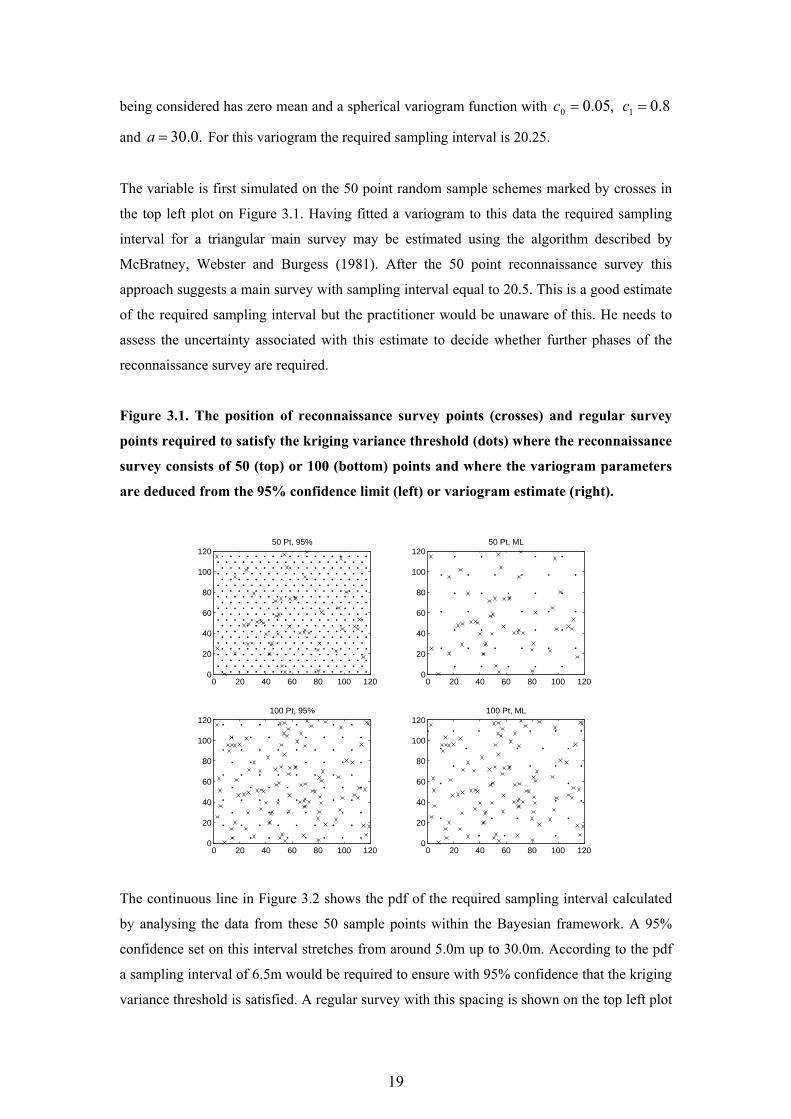
being considered has zero mean and a spherical variogram function with ,05.00 =c 8.01 =c
and .0.30=a For this variogram the required sampling interval is 20.25.
The variable is first simulated on the 50 point random sample schemes marked by crosses in
the top left plot on Figure 3.1. Having fitted a variogram to this data the required sampling
interval for a triangular main survey may be estimated using the algorithm described by
McBratney, Webster and Burgess (1981). After the 50 point reconnaissance survey this
approach suggests a main survey with sampling interval equal to 20.5. This is a good estimate
of the required sampling interval but the practitioner would be unaware of this. He needs to
assess the uncertainty associated with this estimate to decide whether further phases of the
reconnaissance survey are required.
Figure 3.1. The position of reconnaissance survey points (crosses) and regular survey
points required to satisfy the kriging variance threshold (dots) where the reconnaissance
survey consists of 50 (top) or 100 (bottom) points and where the variogram parameters
are deduced from the 95% confidence limit (left) or variogram estimate (right).
0 20 40 60 80 100 1200
20
40
60
80
100
12050 Pt, 95%
0 20 40 60 80 100 1200
20
40
60
80
100
120100 Pt, 95%
0 20 40 60 80 100 1200
20
40
60
80
100
12050 Pt, ML
0 20 40 60 80 100 1200
20
40
60
80
100
120100 Pt, ML
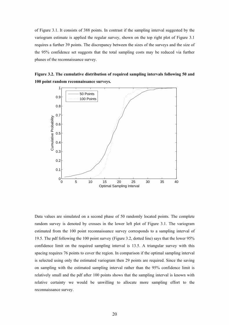
The continuous line in Figure 3.2 shows the pdf of the required sampling interval calculated
by analysing the data from these 50 sample points within the Bayesian framework. A 95%
confidence set on this interval stretches from around 5.0m up to 30.0m. According to the pdf
a sampling interval of 6.5m would be required to ensure with 95% confidence that the kriging
variance threshold is satisfied. A regular survey with this spacing is shown on the top left plot
20
of Figure 3.1. It consists of 388 points. In contrast if the sampling interval suggested by the
variogram estimate is applied the regular survey, shown on the top right plot of Figure 3.1
requires a further 39 points. The discrepancy between the sizes of the surveys and the size of
the 95% confidence set suggests that the total sampling costs may be reduced via further
phases of the reconnaissance survey.
Figure 3.2. The cumulative distribution of required sampling intervals following 50 and
100 point random reconnaissance surveys.
0 5 10 15 20 25 30 35 400
0.1
0.2
0.3
0.4
0.5
0.6
0.7
0.8
0.9
1
Optimal Sampling Interval
Cum
ulat
ive
Pro
babi
lity
50 Points100 Points
Data values are simulated on a second phase of 50 randomly located points. The complete
random survey is denoted by crosses in the lower left plot of Figure 3.1. The variogram
estimated from the 100 point reconnaissance survey corresponds to a sampling interval of
19.5. The pdf following the 100 point survey (Figure 3.2, dotted line) says that the lower 95%
confidence limit on the required sampling interval is 13.5. A triangular survey with this
spacing requires 76 points to cover the region. In comparison if the optimal sampling interval
is selected using only the estimated variogram then 29 points are required. Since the saving
on sampling with the estimated sampling interval rather than the 95% confidence limit is
relatively small and the pdf after 100 points shows that the sampling interval is known with
relative certainty we would be unwilling to allocate more sampling effort to the
reconnaissance survey.
21
Selecting sampling locations in a reconnaissance survey
The above example illustrates how the data collected in a reconnaissance survey may be
interpreted within a Bayesian framework in order to decide when the required sampling
interval is with enough precision to start the main survey. The position of the sample points
are selected at random. In this section we describe how the position of sample points may be
optimized in order to learn about the required sampling interval with as few sample points as
possible. In Chapter 2 we saw that the nature of an optimal sampling scheme for variogram
estimation depends on the variogram being estimated. In particular if the range of spatial
correlation is reduced more comparisons between close pairs of points are required.
We design reconnaissance surveys to minimize the uncertainty in the estimate of the required
sampling interval. This uncertainty depends upon the variogram of the variable being
measured. Since we can only estimate this variogram we express the uncertainty in the
required sampling interval in terms of the pdf of the variogram parameters. This pdf is re-
calculated after each phase of sampling. Thus the sample scheme varies according to the data
collected from earlier phases in the reconnaissance survey. We refer to such sample schemes
as Bayesian adaptive schemes.
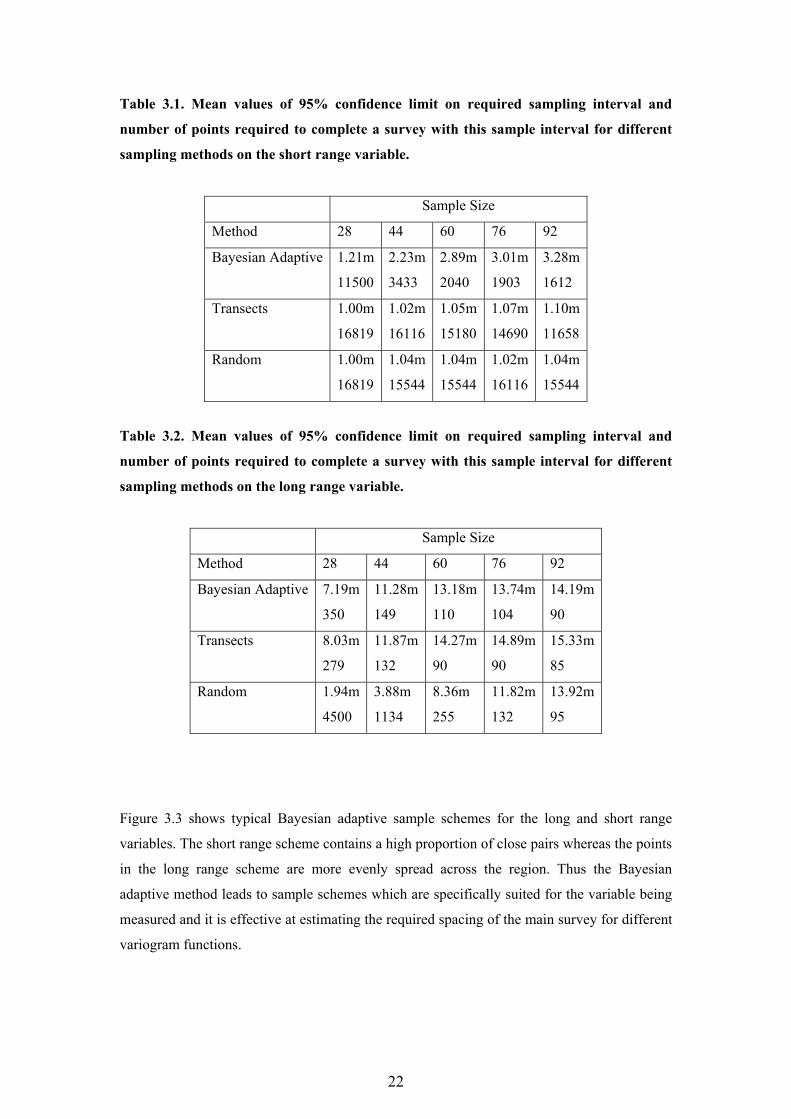
Tables 3.1 and 3.2 compare the performance of Bayesian adaptive schemes with random
schemes and regular transects for variables with a short and long range of spatial correlation.
Each transect is randomly positioned in the region and contains eight points separated by
10m. The mean value of the lower 95% confidence limit on the required sampling interval
and the number of sample points required to complete a triangular survey with this interval,
are shown for sample schemes of different sizes. For the short range variable the 95%
confidence limit from the Bayesian adaptive scheme is greater than those from the random
and transect schemes and the sampling load required to complete the survey is considerably
less. In many cases the random and transect schemes do not increase this confidence limit
above the minimum permitted value of 1.0.
There is much less difference in the performance of the schemes for the long range variable
although the transect scheme has slightly greater confidence limits than the Bayesian adaptive
scheme which are in turn slightly greater than those from random schemes. A relatively small
number of points are required to survey this variable – a fact which the Bayesian adaptive
scheme is able to identify, thus avoiding over-sampling.
22
Table 3.1. Mean values of 95% confidence limit on required sampling interval and
number of points required to complete a survey with this sample interval for different
sampling methods on the short range variable.
Sample Size
Method 28 44 60 76 92
Bayesian Adaptive 1.21m
11500
2.23m
3433
2.89m
2040
3.01m
1903
3.28m
1612
Transects 1.00m
16819
1.02m
16116
1.05m
15180
1.07m
14690
1.10m
11658
Random 1.00m
16819
1.04m
15544
1.04m
15544
1.02m
16116
1.04m
15544
Table 3.2. Mean values of 95% confidence limit on required sampling interval and
number of points required to complete a survey with this sample interval for different
sampling methods on the long range variable.
Sample Size
Method 28 44 60 76 92
Bayesian Adaptive 7.19m
350
11.28m
149
13.18m
110
13.74m
104
14.19m
90
Transects 8.03m
279
11.87m
132
14.27m
90
14.89m
90
15.33m
85
Random 1.94m
4500
3.88m
1134
8.36m
255
11.82m
132
13.92m
95
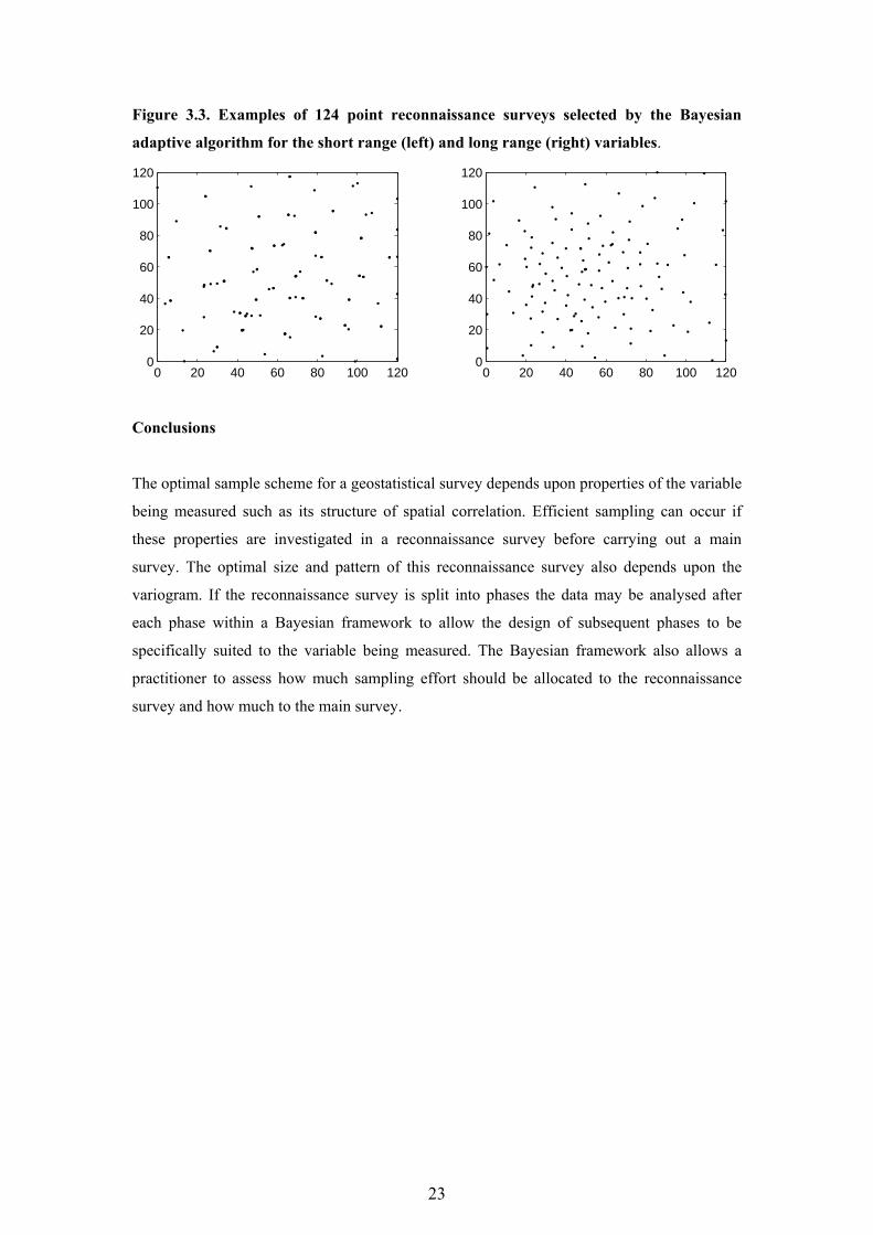
Figure 3.3 shows typical Bayesian adaptive sample schemes for the long and short range
variables. The short range scheme contains a high proportion of close pairs whereas the points
in the long range scheme are more evenly spread across the region. Thus the Bayesian
adaptive method leads to sample schemes which are specifically suited for the variable being
measured and it is effective at estimating the required spacing of the main survey for different
variogram functions.
23
Figure 3.3. Examples of 124 point reconnaissance surveys selected by the Bayesian
adaptive algorithm for the short range (left) and long range (right) variables.
0 20 40 60 80 100 1200
20
40
60
80
100
120
0 20 40 60 80 100 1200
20
40
60
80
100
120
Conclusions
The optimal sample scheme for a geostatistical survey depends upon properties of the variable
being measured such as its structure of spatial correlation. Efficient sampling can occur if
these properties are investigated in a reconnaissance survey before carrying out a main
survey. The optimal size and pattern of this reconnaissance survey also depends upon the
variogram. If the reconnaissance survey is split into phases the data may be analysed after
each phase within a Bayesian framework to allow the design of subsequent phases to be
specifically suited to the variable being measured. The Bayesian framework also allows a
practitioner to assess how much sampling effort should be allocated to the reconnaissance
survey and how much to the main survey.
24
CHAPTER 4. A FIELD SYSTEM FOR ADAPTIVE SAMPLING
Introduction
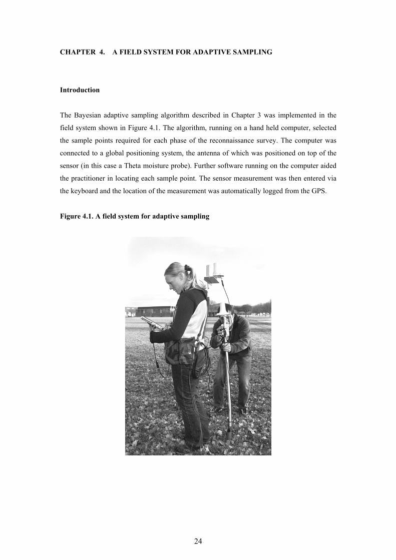
The Bayesian adaptive sampling algorithm described in Chapter 3 was implemented in the
field system shown in Figure 4.1. The algorithm, running on a hand held computer, selected
the sample points required for each phase of the reconnaissance survey. The computer was
connected to a global positioning system, the antenna of which was positioned on top of the
sensor (in this case a Theta moisture probe). Further software running on the computer aided
the practitioner in locating each sample point. The sensor measurement was then entered via
the keyboard and the location of the measurement was automatically logged from the GPS.
Figure 4.1. A field system for adaptive sampling
25
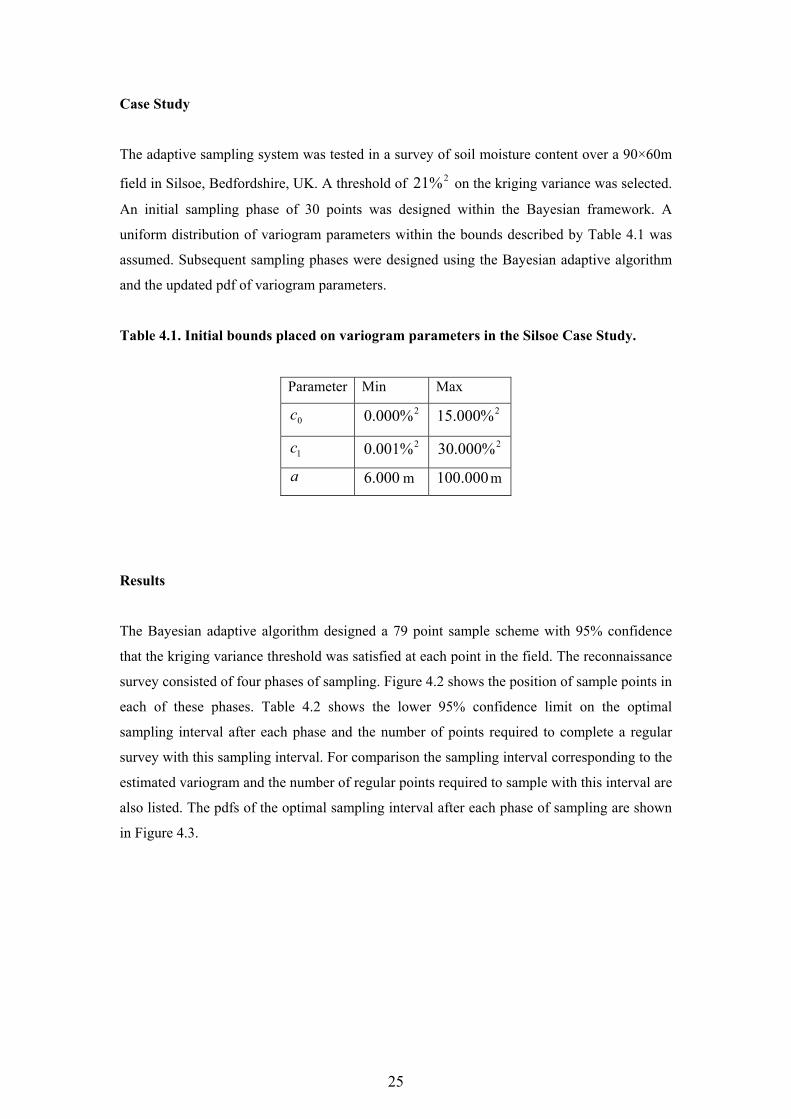
Case Study
The adaptive sampling system was tested in a survey of soil moisture content over a 90×60m
field in Silsoe, Bedfordshire, UK. A threshold of 2%21 on the kriging variance was selected.
An initial sampling phase of 30 points was designed within the Bayesian framework. A
uniform distribution of variogram parameters within the bounds described by Table 4.1 was
assumed. Subsequent sampling phases were designed using the Bayesian adaptive algorithm
and the updated pdf of variogram parameters.
Table 4.1. Initial bounds placed on variogram parameters in the Silsoe Case Study.
Parameter Min Max
0c 2%000.0 2%000.15
1c 2%001.0 2%000.30
a 000.6 m 000.100 m
Results
The Bayesian adaptive algorithm designed a 79 point sample scheme with 95% confidence
that the kriging variance threshold was satisfied at each point in the field. The reconnaissance
survey consisted of four phases of sampling. Figure 4.2 shows the position of sample points in
each of these phases. Table 4.2 shows the lower 95% confidence limit on the optimal
sampling interval after each phase and the number of points required to complete a regular
survey with this sampling interval. For comparison the sampling interval corresponding to the
estimated variogram and the number of regular points required to sample with this interval are
also listed. The pdfs of the optimal sampling interval after each phase of sampling are shown
in Figure 4.3.
26
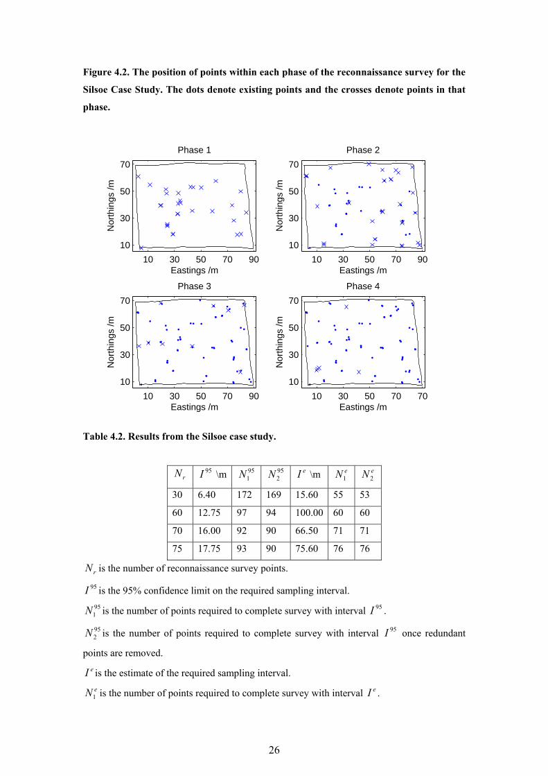
Figure 4.2. The position of points within each phase of the reconnaissance survey for the
Silsoe Case Study. The dots denote existing points and the crosses denote points in that
phase.
10 30 50 70 90
10
30
50
70
Phase 1
Eastings /m
Nor
thin
gs /m
10 30 50 70 90
10
30
50
70
Phase 2
Eastings /mN
orth
ings
/m
10 30 50 70 90
10
30
50
70
Phase 3
Eastings /m
Nor
thin
gs /m
10 30 50 70 70
10
30
50
70
Phase 4
Eastings /m
Nor
thin
gs /m
Table 4.2. Results from the Silsoe case study.
rN 95I \m 951N 95
2N eI \m eN1eN2
30 6.40 172 169 15.60 55 53
60 12.75 97 94 100.00 60 60
70 16.00 92 90 66.50 71 71
75 17.75 93 90 75.60 76 76
rN is the number of reconnaissance survey points.
95I is the 95% confidence limit on the required sampling interval. 951N is the number of points required to complete survey with interval 95I .
952N is the number of points required to complete survey with interval 95I once redundant
points are removed. eI is the estimate of the required sampling interval.
eN1 is the number of points required to complete survey with interval eI .
27
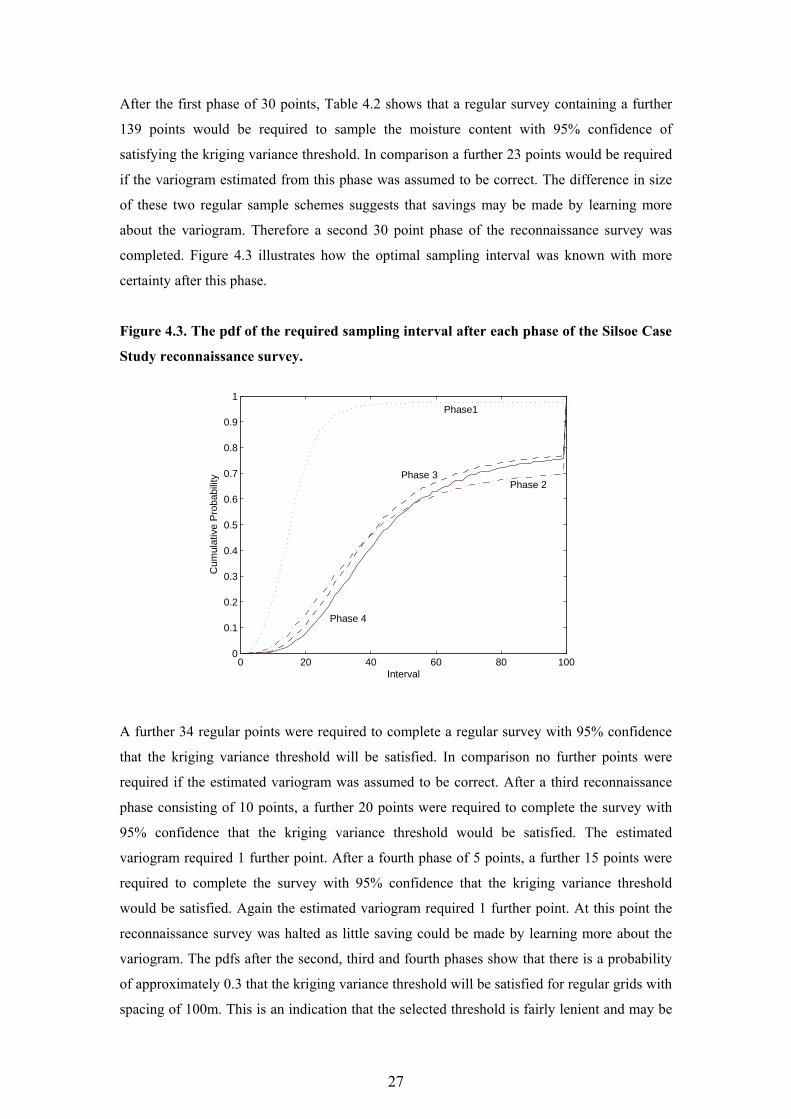
After the first phase of 30 points, Table 4.2 shows that a regular survey containing a further
139 points would be required to sample the moisture content with 95% confidence of
satisfying the kriging variance threshold. In comparison a further 23 points would be required
if the variogram estimated from this phase was assumed to be correct. The difference in size
of these two regular sample schemes suggests that savings may be made by learning more
about the variogram. Therefore a second 30 point phase of the reconnaissance survey was
completed. Figure 4.3 illustrates how the optimal sampling interval was known with more
certainty after this phase.
Figure 4.3. The pdf of the required sampling interval after each phase of the Silsoe Case
Study reconnaissance survey.
0 20 40 60 80 1000
0.1
0.2
0.3
0.4
0.5
0.6
0.7
0.8
0.9
1
Interval
Cum
ulat
ive
Pro
babi
lity
Phase1
Phase 3Phase 2
Phase 4
A further 34 regular points were required to complete a regular survey with 95% confidence
that the kriging variance threshold will be satisfied. In comparison no further points were
required if the estimated variogram was assumed to be correct. After a third reconnaissance
phase consisting of 10 points, a further 20 points were required to complete the survey with
95% confidence that the kriging variance threshold would be satisfied. The estimated
variogram required 1 further point. After a fourth phase of 5 points, a further 15 points were
required to complete the survey with 95% confidence that the kriging variance threshold
would be satisfied. Again the estimated variogram required 1 further point. At this point the
reconnaissance survey was halted as little saving could be made by learning more about the
variogram. The pdfs after the second, third and fourth phases show that there is a probability
of approximately 0.3 that the kriging variance threshold will be satisfied for regular grids with
spacing of 100m. This is an indication that the selected threshold is fairly lenient and may be
28
greater than the total variance of the moisture content across the field. For this reason a
relatively small number of points are required to complete the survey. A non adaptive
sampling scheme would not have recognised this, possibly leading to over-sampling of the
region.
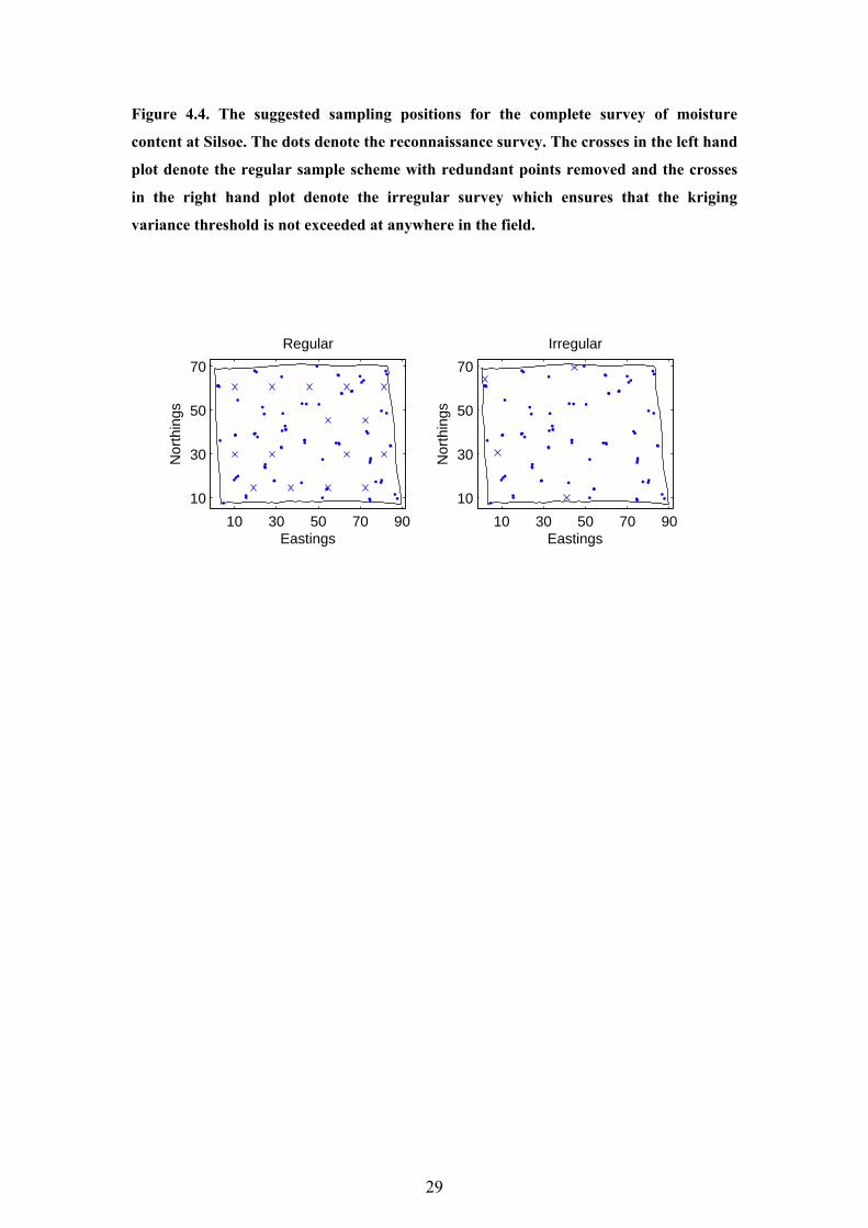
The left hand plot in Figure 4.4 shows the 75 point reconnaissance survey and the 15 points
on the regular grid suggested by the adaptive algorithm. The sample size may be reduced
further by permitting irregularly positioned points in the main survey. In the right hand plot of
Figure 4.4, the 15 regular points have been replaced by four irregularly positioned points. The
number and position of these points were chosen using an iterative spatial simulated
annealing algorithm designed to ensure that the kriging variance threshold was satisfied
everywhere in the field. This algorithm used the most probable of the sets of variogram
parameters which corresponded to a sampling interval equal to the lower 95% confidence
limit. Initially a SSA algorithm was used to minimize the maximum kriging variance within
the region with 15 points in addition to the reconnaissance survey points (van Groenigen,
1999). If the maximum kriging variance threshold was satisfied one point was removed and
the SSA algorithm was repeated. This process continued until there were insufficient points to
satisfy the kriging variance threshold. The four points shown on the right hand plot of Figure
4.4 represent the position of the smallest number of points able to satisfy the kriging variance
threshold.
Conclusions The Bayesian adaptive algorithm for reconnaissance surveys was successfully implemented
into a field system. This system was used to design a survey to map soil moisture content over
a field with 95% confidence that a threshold placed on the kriging variance was satisfied
everywhere in the field. The survey is specifically suited to the variable being measured and
the threshold placed on it; the relatively small number of points required indicates that the
threshold may have been almost as large as the total variance of the moisture content.
29
Figure 4.4. The suggested sampling positions for the complete survey of moisture
content at Silsoe. The dots denote the reconnaissance survey. The crosses in the left hand
plot denote the regular sample scheme with redundant points removed and the crosses
in the right hand plot denote the irregular survey which ensures that the kriging
variance threshold is not exceeded at anywhere in the field.
10 30 50 70 90
10
30
50
70
Regular
Eastings
Nor
thin
gs
10 30 50 70 90
10
30
50
70
Irregular
Eastings
Nor
thin
gs

30
Acknowledgements
We are grateful to the Agri-Food committee of the BBSRC for funding this project (85%)
through grant 204/D15335. Mr Peter Richards contributed to the design of the field system.
31
References
Brus, D.J., Spätjens, L.E.E.M. and de Gruitjer, J.J. (1999). A sampling scheme for estimating the mean extractable phosphorus concentration of fields for environmental regulation. Geoderma, 89, 129–148. Hague, T., Marchant, J.A. and Tillett, N.D. (2000). Ground based sensing systems for autonomous agricultural vehicles. Computers and Electronics in Agriculture, 25, 11-28. Lark, R.M. (2002). Optimized spatial sampling of soil for estimation of the variogram by maximum likelihood. Geoderma, 105, 49–80. McBratney, A.B., Webster, R. and Burgess, T.M. (1981). The design of optimal sampling schemes for local estimation and mapping of regionalised variables. Computers and Geosciences, 7, 331–334. Miller AJ, Wells DM, Braven J, Ebdon L, Le Goff T, Clark LJ, Whalley WR, Gowing DJG and Leeds-Harrison PB (2003). Novel Sensors for Measuring Soil Nitrogen, Water Availability and Strength. Proceedings of the British Society for Crop Protection International Congress, Glasgow. pp. 1107–1114. Pardo-Igqúzquiza, E. and Dowd, P.A. (2003). Assessment of the uncertainty of spatial covariance parameters of soil properties and its use in applications. Soil Science, 168, 769–782. Van Groenigen, J.W. (1999). Constrained optimisation of spatial sampling: ITC Publication Series, v.65, Enschede. Viscarra Rossel, R.A. and McBratney, A.B. (2000). A two-factor empirical deterministic response surface calibration model for site-specific predictions of lime requirement. Precision Agriculture 2, 163–178. Zimmerman, D.L. and Cressie, N. (1992). Mean squared prediction error in the spatial linear model with estimated covariance parameters. Annals of the Institute of Statistical Mathematics 44, 27–43.