Embed Size (px)
Citation preview
1-1
How Bad is Selfish Routing
Tim Roughgarden Eva Tardos
presented by Yajun Wang ([email protected])
for COMP670O Spring 2006, HKUST
2-1
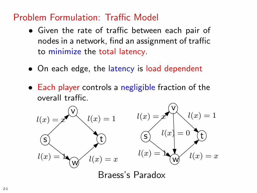
Problem Formulation: Traffic Model
• Given the rate of traffic between each pair ofnodes in a network, find an assignment of trafficto minimize the total latency.
• On each edge, the latency is load dependent
v
s t
w
l(x) = x
l(x) = xl(x) = 1
l(x) = 1
v
s t
w
l(x) = x
l(x) = xl(x) = 1
l(x) = 1
l(x) = 0
Braess’s Paradox
• Each player controls a negligible fraction of theoverall traffic.
3-1
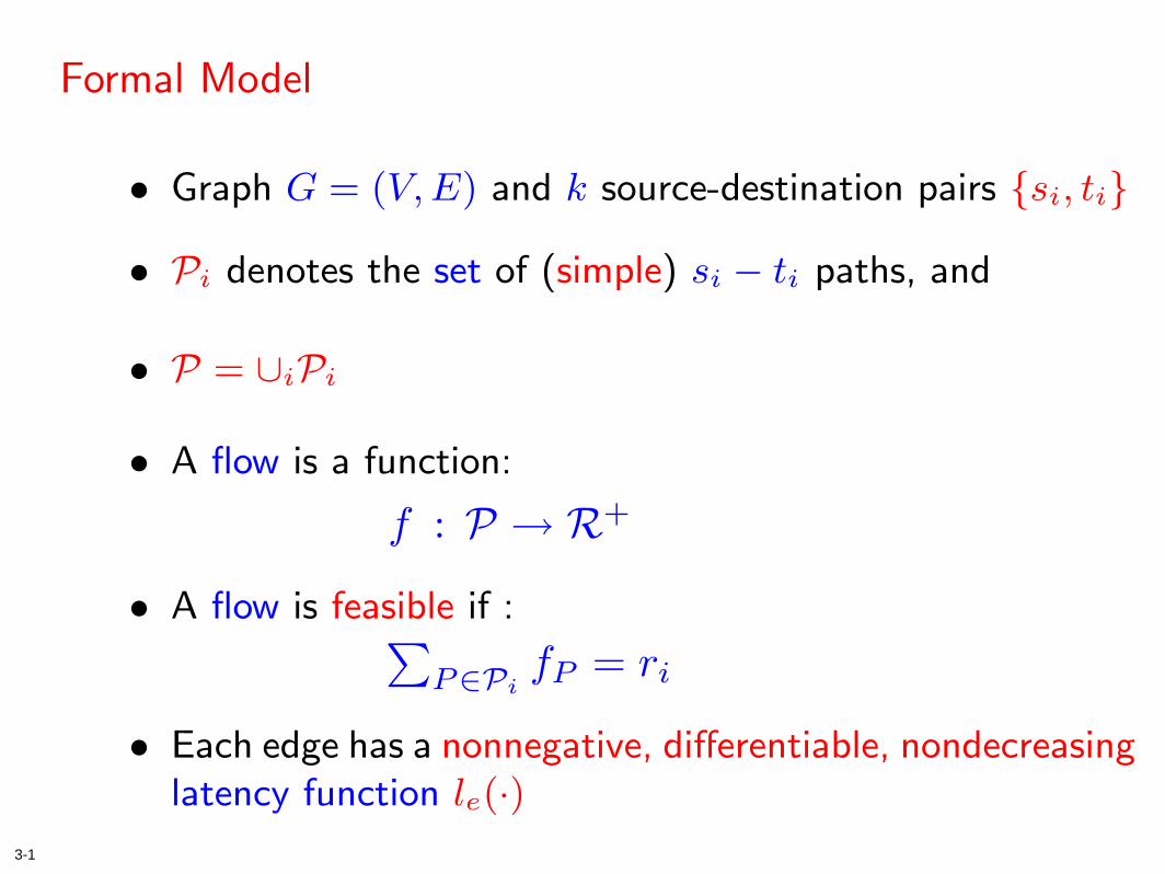
Formal Model
• Graph G = (V, E) and k source-destination pairs {si, ti}
• P = ∪iPi
• Pi denotes the set of (simple) si − ti paths, and
• A flow is a function:
f : P → R+
• A flow is feasible if :∑P∈Pi
fP = ri
• Each edge has a nonnegative, differentiable, nondecreasinglatency function le(·)
4-1
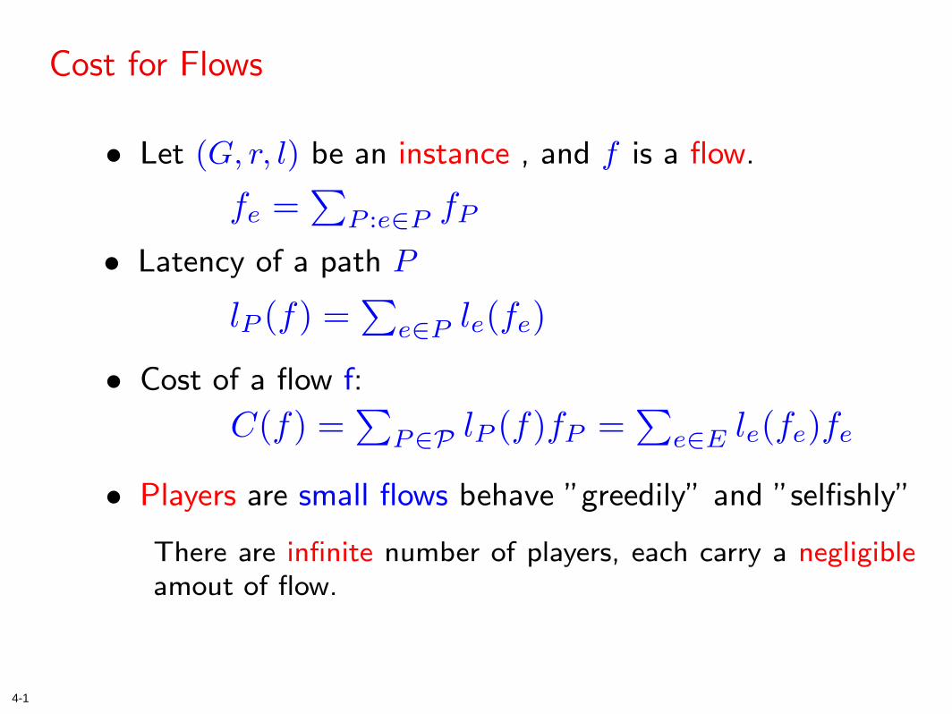
Cost for Flows
• Let (G, r, l) be an instance , and f is a flow.
• Latency of a path P
• Cost of a flow f:
• Players are small flows behave ”greedily” and ”selfishly”
lP (f) =∑
e∈P le(fe)
C(f) =∑
P∈P lP (f)fP =∑
e∈E le(fe)fe
There are infinite number of players, each carry a negligibleamout of flow.
fe =∑
P :e∈P fP
5-1
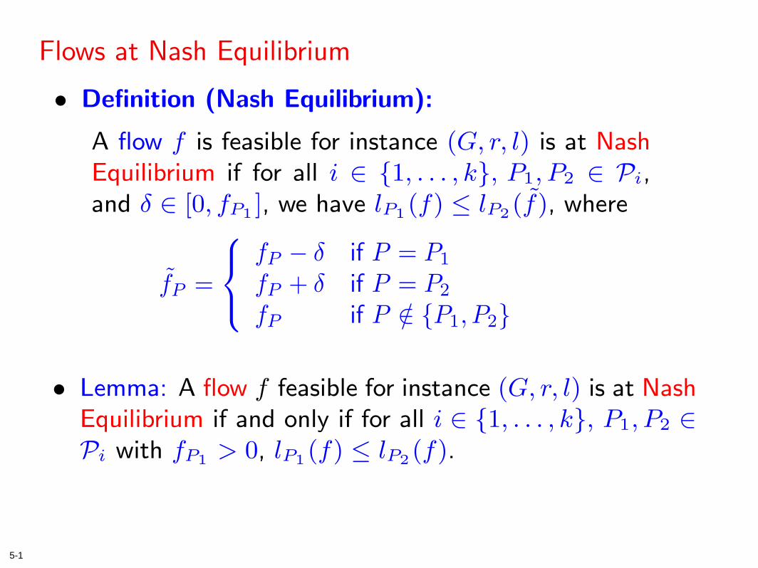
Flows at Nash Equilibrium
• Definition (Nash Equilibrium):
A flow f is feasible for instance (G, r, l) is at NashEquilibrium if for all i ∈ {1, . . . , k}, P1, P2 ∈ Pi,and δ ∈ [0, fP1 ], we have lP1(f) ≤ lP2(f̃), where
f̃P =
fP − δ if P = P1
fP + δ if P = P2
fP if P /∈ {P1, P2}
• Lemma: A flow f feasible for instance (G, r, l) is at NashEquilibrium if and only if for all i ∈ {1, . . . , k}, P1, P2 ∈Pi with fP1 > 0, lP1(f) ≤ lP2(f).
6-1
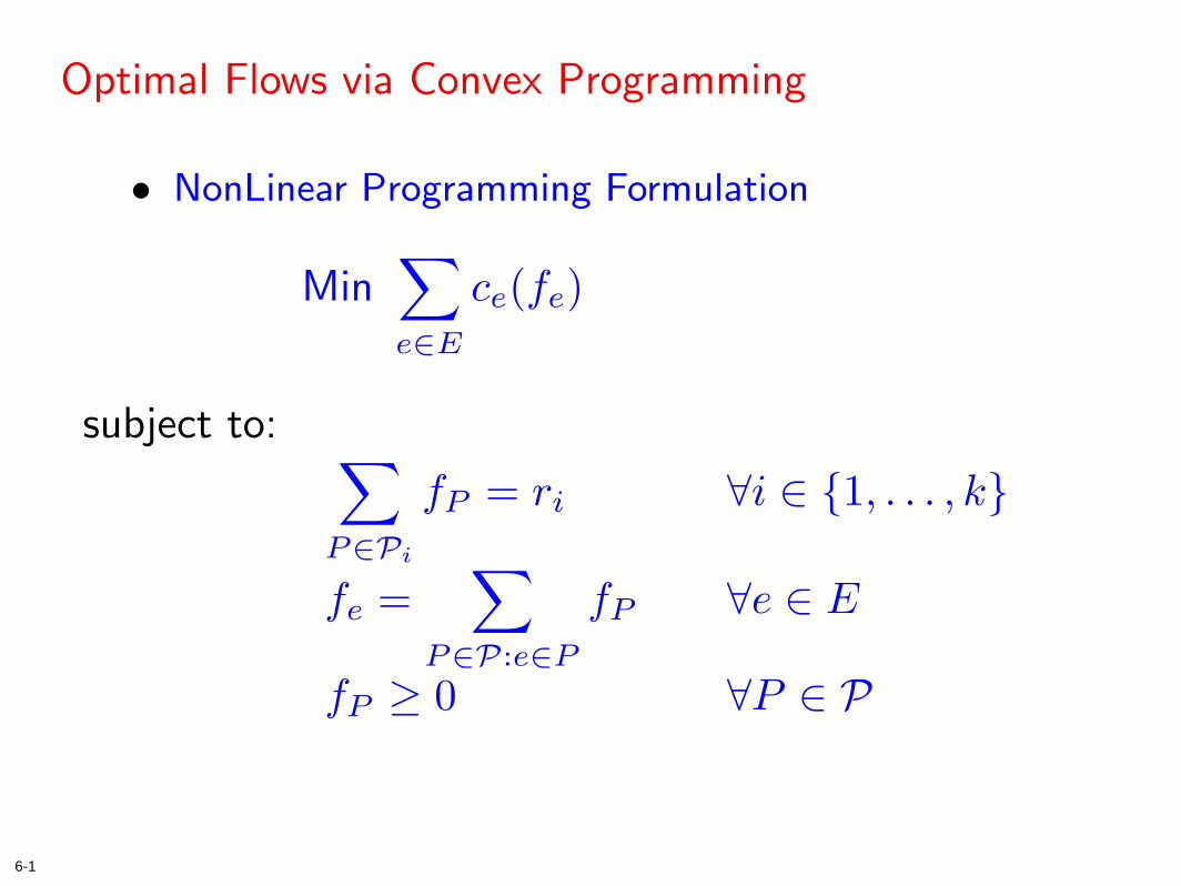
Optimal Flows via Convex Programming
• NonLinear Programming Formulation
∑P∈Pi
fP = ri ∀i ∈ {1, . . . , k}
fe =∑
P∈P:e∈P
fP ∀e ∈ E
fP ≥ 0 ∀P ∈ P
Min∑e∈E
ce(fe)
subject to:

7-1
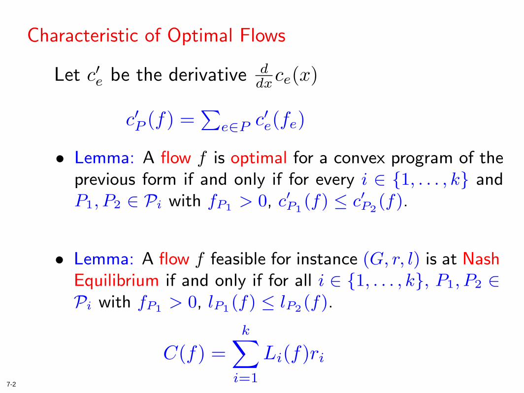
Characteristic of Optimal Flows
• Lemma: A flow f is optimal for a convex program of theprevious form if and only if for every i ∈ {1, . . . , k} andP1, P2 ∈ Pi with fP1 > 0, c′P1(f) ≤ c′P2(f).
c′P (f) =∑
e∈P c′e(fe)
Let c′e be the derivative ddxce(x)
7-2
Characteristic of Optimal Flows
• Lemma: A flow f is optimal for a convex program of theprevious form if and only if for every i ∈ {1, . . . , k} andP1, P2 ∈ Pi with fP1 > 0, c′P1(f) ≤ c′P2(f).
c′P (f) =∑
e∈P c′e(fe)
Let c′e be the derivative ddxce(x)
• Lemma: A flow f feasible for instance (G, r, l) is at NashEquilibrium if and only if for all i ∈ {1, . . . , k}, P1, P2 ∈Pi with fP1 > 0, lP1(f) ≤ lP2(f).
C(f) =k∑
i=1
Li(f)ri
8-1
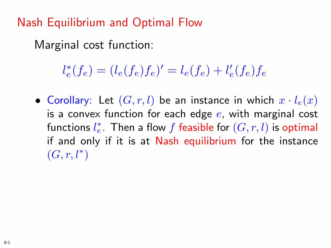
Nash Equilibrium and Optimal Flow
• Corollary: Let (G, r, l) be an instance in which x · le(x)is a convex function for each edge e, with marginal costfunctions l∗e . Then a flow f feasible for (G, r, l) is optimalif and only if it is at Nash equilibrium for the instance(G, r, l∗)
l∗e(fe) = (le(fe)fe)′ = le(fe) + l′e(fe)fe
Marginal cost function:
9-1
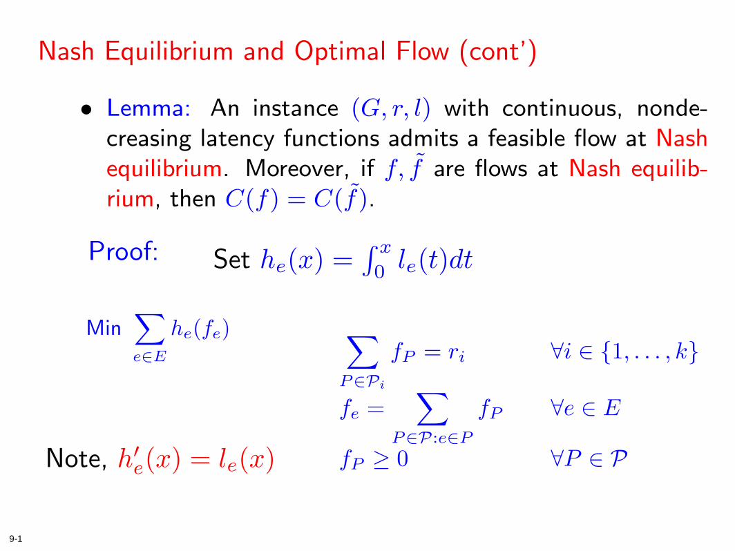
Nash Equilibrium and Optimal Flow (cont’)
• Lemma: An instance (G, r, l) with continuous, nonde-creasing latency functions admits a feasible flow at Nashequilibrium. Moreover, if f, f̃ are flows at Nash equilib-rium, then C(f) = C(f̃).
Proof:
∑P∈Pi
fP = ri ∀i ∈ {1, . . . , k}
fe =∑
P∈P:e∈P
fP ∀e ∈ E
fP ≥ 0 ∀P ∈ P
Min∑e∈E
he(fe)
Set he(x) =∫ x
0le(t)dt
Note, h′e(x) = le(x)
10-1
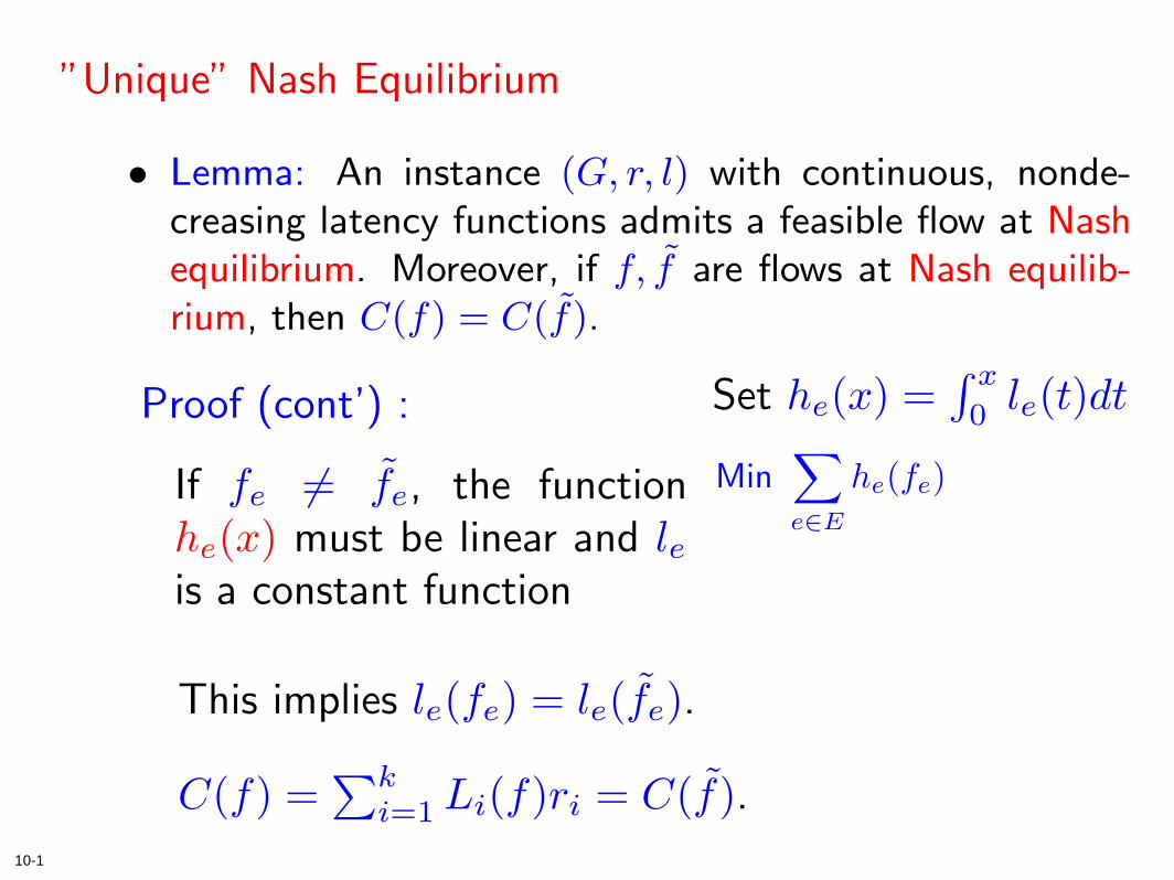
”Unique” Nash Equilibrium
• Lemma: An instance (G, r, l) with continuous, nonde-creasing latency functions admits a feasible flow at Nashequilibrium. Moreover, if f, f̃ are flows at Nash equilib-rium, then C(f) = C(f̃).
Proof (cont’) :
Min∑e∈E
he(fe)
Set he(x) =∫ x
0le(t)dt
If fe 6= f̃e, the functionhe(x) must be linear and leis a constant function
This implies le(fe) = le(f̃e).
C(f) =∑k
i=1 Li(f)ri = C(f̃).
11-1
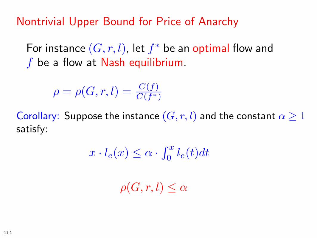
Nontrivial Upper Bound for Price of Anarchy
ρ = ρ(G, r, l) = C(f)C(f∗)
ρ(G, r, l) ≤ α
For instance (G, r, l), let f∗ be an optimal flow andf be a flow at Nash equilibrium.
Corollary: Suppose the instance (G, r, l) and the constant α ≥ 1satisfy:
x · le(x) ≤ α ·∫ x
0le(t)dt
12-1
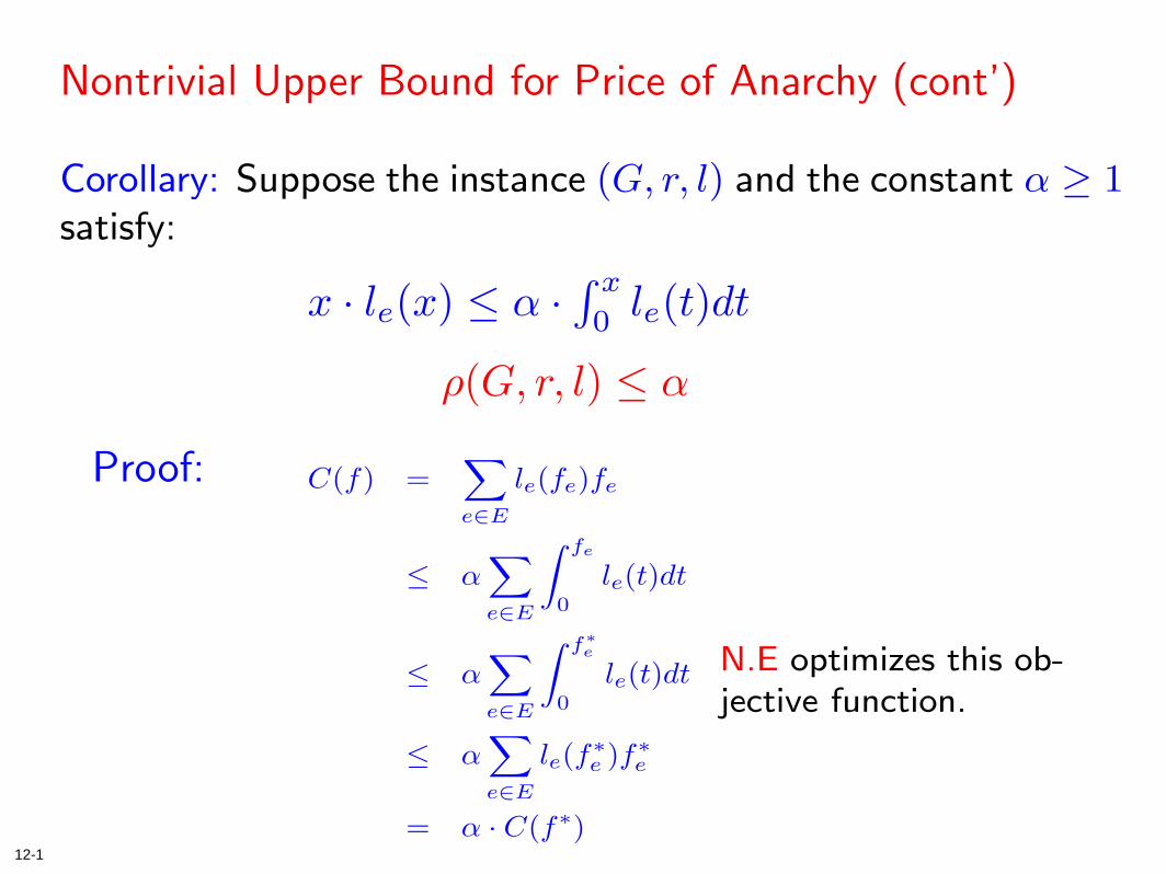
Nontrivial Upper Bound for Price of Anarchy (cont’)
ρ(G, r, l) ≤ α
Corollary: Suppose the instance (G, r, l) and the constant α ≥ 1satisfy:
x · le(x) ≤ α ·∫ x
0le(t)dt
Proof: C(f) =∑e∈E
le(fe)fe
≤ α∑e∈E
∫ fe
0
le(t)dt
≤ α∑e∈E
∫ f∗e
0
le(t)dt
≤ α∑e∈E
le(f∗e )f∗e
= α · C(f∗)
N.E optimizes this ob-jective function.
13-1
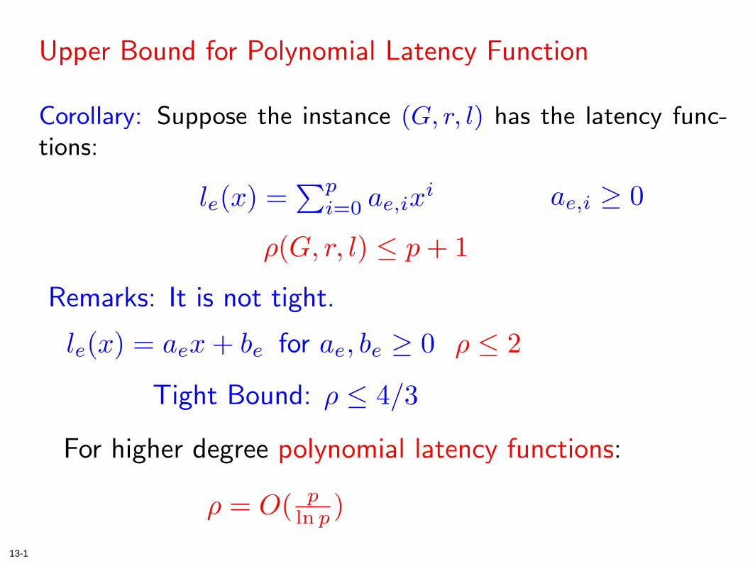
Upper Bound for Polynomial Latency Function
ρ(G, r, l) ≤ p + 1
Corollary: Suppose the instance (G, r, l) has the latency func-tions:
le(x) =∑p
i=0 ae,ixi
Remarks: It is not tight.
ae,i ≥ 0
le(x) = aex + be for ae, be ≥ 0 ρ ≤ 2
For higher degree polynomial latency functions:
ρ = O( pln p )
Tight Bound: ρ ≤ 4/3
14-1
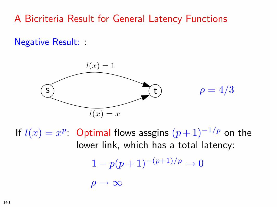
A Bicriteria Result for General Latency Functions
Negative Result: :
If l(x) = xp:
1− p(p + 1)−(p+1)/p → 0
s t
l(x) = 1
l(x) = x
ρ = 4/3
Optimal flows assgins (p+1)−1/p on thelower link, which has a total latency:
ρ →∞
15-1
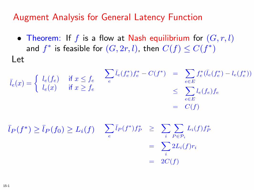
Augment Analysis for General Latency Function
Let
• Theorem: If f is a flow at Nash equilibrium for (G, r, l)and f∗ is feasible for (G, 2r, l), then C(f) ≤ C(f∗)
l̄e(x) ={
le(fe) if x ≤ fe
le(x) if x ≥ fe
∑e
l̄e(f∗e )f∗e − C(f∗) =∑e∈E
f∗e (l̄e(f∗e )− le(f∗e ))
≤∑e∈E
le(fe)fe
= C(f)
∑e
l̄P (f∗)f∗P ≥∑
i
∑P∈Pi
Li(f)f∗P
=∑
i
2Li(f)ri
= 2C(f)
l̄P (f∗) ≥ l̄P (f0) ≥ Li(f)
16-1
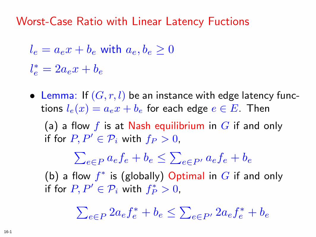
Worst-Case Ratio with Linear Latency Fuctions
• Lemma: If (G, r, l) be an instance with edge latency func-tions le(x) = aex + be for each edge e ∈ E. Then
le = aex + be with ae, be ≥ 0
l∗e = 2aex + be
(a) a flow f is at Nash equilibrium in G if and onlyif for P, P ′ ∈ Pi with fP > 0,∑
e∈P aefe + be ≤∑
e∈P ′ aefe + be
(b) a flow f∗ is (globally) Optimal in G if and onlyif for P, P ′ ∈ Pi with f∗P > 0,∑
e∈P 2aef∗e + be ≤
∑e∈P ′ 2aef
∗e + be
17-1
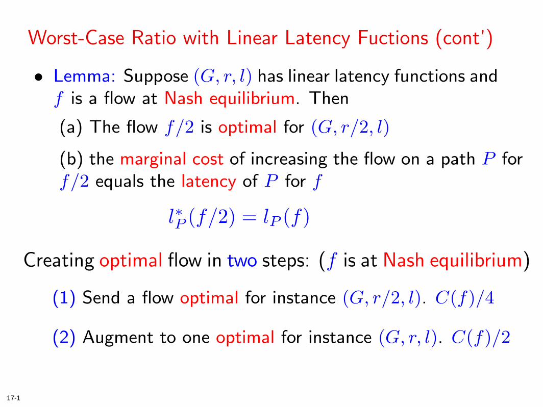
Worst-Case Ratio with Linear Latency Fuctions (cont’)
• Lemma: Suppose (G, r, l) has linear latency functions andf is a flow at Nash equilibrium. Then
(a) The flow f/2 is optimal for (G, r/2, l)
(b) the marginal cost of increasing the flow on a path P forf/2 equals the latency of P for f
Creating optimal flow in two steps: (f is at Nash equilibrium)
(1) Send a flow optimal for instance (G, r/2, l). C(f)/4
(2) Augment to one optimal for instance (G, r, l). C(f)/2
l∗P (f/2) = lP (f)
18-1
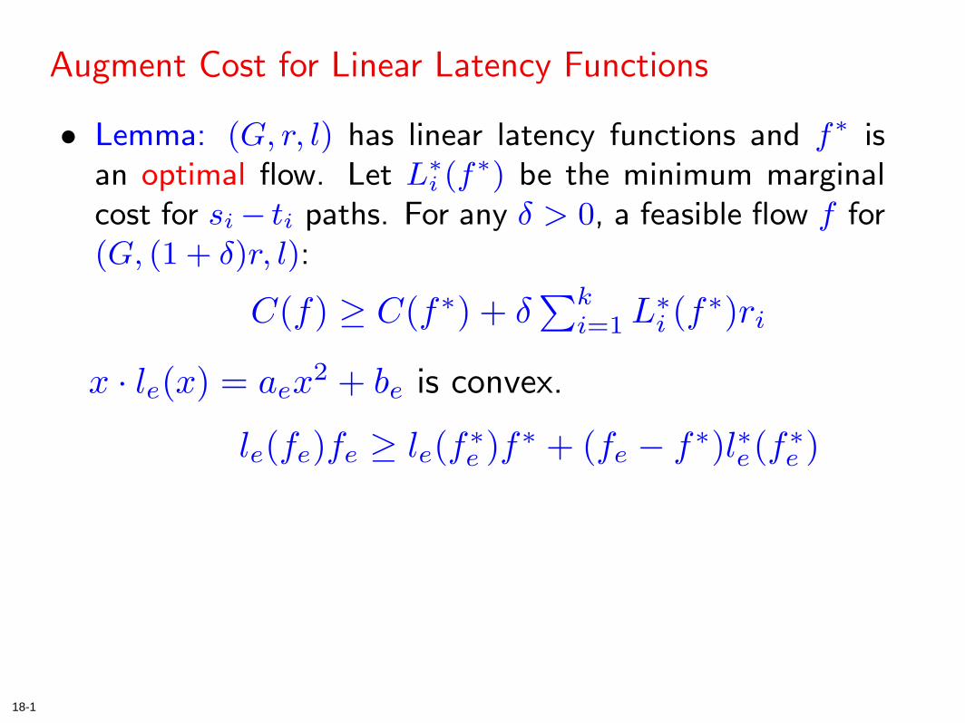
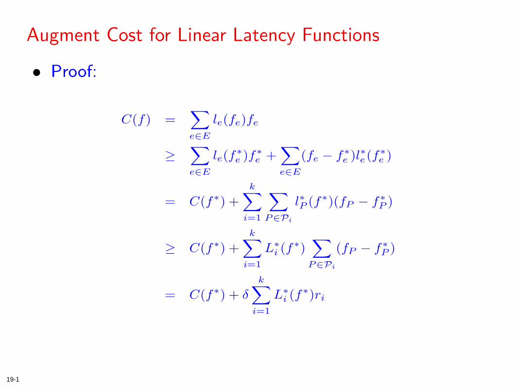
Augment Cost for Linear Latency Functions
• Lemma: (G, r, l) has linear latency functions and f∗ isan optimal flow. Let L∗
i (f∗) be the minimum marginal
cost for si− ti paths. For any δ > 0, a feasible flow f for(G, (1 + δ)r, l):
x · le(x) = aex2 + be is convex.
C(f) ≥ C(f∗) + δ∑k
i=1 L∗i (f
∗)ri
le(fe)fe ≥ le(f∗e )f∗ + (fe − f∗)l∗e(f∗e )
19-1
Augment Cost for Linear Latency Functions
• Proof:
C(f) =∑e∈E
le(fe)fe
≥∑e∈E
le(f∗e )f∗e +∑e∈E
(fe − f∗e )l∗e(f∗e )
= C(f∗) +k∑
i=1
∑P∈Pi
l∗P (f∗)(fP − f∗P )
≥ C(f∗) +k∑
i=1
L∗i (f
∗)∑
P∈Pi
(fP − f∗P )
= C(f∗) + δk∑
i=1
L∗i (f
∗)ri
20-1
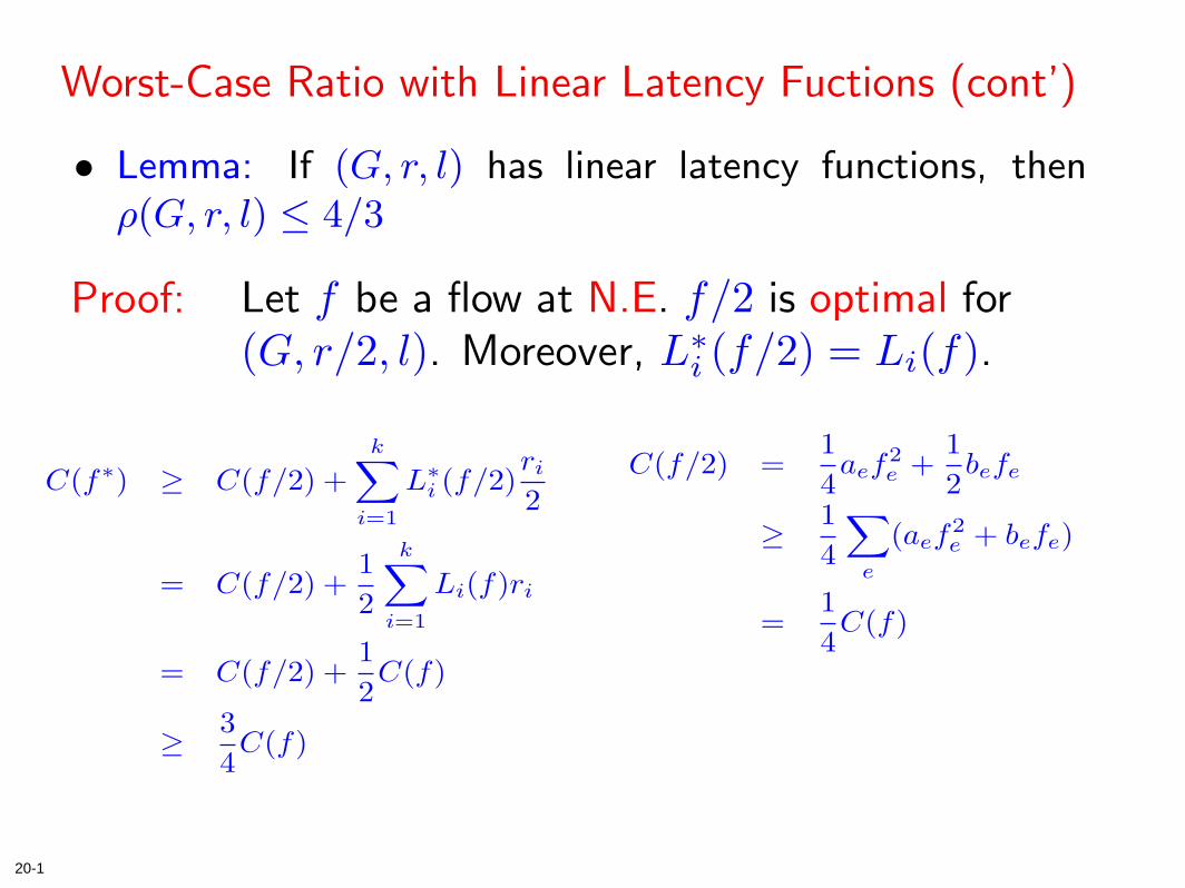
Worst-Case Ratio with Linear Latency Fuctions (cont’)
• Lemma: If (G, r, l) has linear latency functions, thenρ(G, r, l) ≤ 4/3
Let f be a flow at N.E. f/2 is optimal for(G, r/2, l). Moreover, L∗
i (f/2) = Li(f).Proof:
C(f∗) ≥ C(f/2) +k∑
i=1
L∗i (f/2)
ri
2
= C(f/2) +12
k∑i=1
Li(f)ri
= C(f/2) +12C(f)
≥ 34C(f)
C(f/2) =14aef
2e +
12befe
≥ 14
∑e
(aef2e + befe)
=14C(f)
21-1
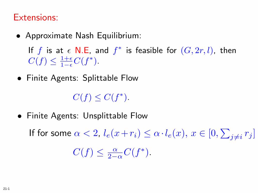
Extensions:
• Approximate Nash Equilibrium:
If f is at ε N.E, and f∗ is feasible for (G, 2r, l), thenC(f) ≤ 1+ε
1−εC(f∗).
• Finite Agents: Splittable Flow
C(f) ≤ C(f∗).
• Finite Agents: Unsplittable Flow
If for some α < 2, le(x+ri) ≤ α · le(x), x ∈ [0,∑
j 6=i rj ]
C(f) ≤ α2−αC(f∗).