Embed Size (px)
Citation preview
kTECHNOLOG1CAL FORECASTING AND SOCIAL CHANGE 46,153-173 (1-
Determination of the Uncertainties in S-Curve Logistic Fits
A. DEBECKER AND T. MODIS
ABSTRACT
Look-up tables and graphs are provided for determining the uncertainties during logistic fits, on the three parameters M, a and to describing an S-curve of the form:
The uncertainties and the associated confidence levels are given as a function of the uncertainty on the data points and the length of the historical period. Correlations between these variables are also examined; they make “what-if’ games possible even before doing the fit.
The study is based on some 35,000 S-curve fits on simulated data covering a variety of conditions and carried out via a x2 minimization technique. A rule-of-thumb general result is that, given at least half of the S-curve range and a precision of better than 10% on each hitorical point, the uncertainty on M will be less than 20% with 90% confidence level.
Introduction S-curve logistic fitting has been successful in describing learning and/or growing
processes. A variety of applications ranging from biology (echo-niche filling of species) to art and industry (market-niche filling of products) abounds in the literature [l-41.
The most facinating aspect of S-curve fitting is the ability to predict from early measurements the final maximum, a fact that often shocks and sometimes vexes individu- als, with its inherent element of predeterminism. This very fact, however, constitutes also the fundamental weakness and the major criticism in S-curve fitting, namely the uncertainty involved in an early determination of the final maximum. A three-parameter logistic fit can sometimes accomodate wildly different values for the final maximum. Obviously, the more precise the data and the more of the S-curve range they cover, the more accurate the determination of the final maximum but, unfortunately, at the same time, the less interesting this determination becomes.
The need for quantitative determination of the uncertainties resulting from such fits has not been adequately addressed up to now. In this work a study was undertaken to quantify the uncertainties on the parameters determined by logistic S-curve fits.
THEODORE MODIS is a physicist and a senior management strategy consultant at Digital Equipment Co. He has taught at Columbia University, New York, NY; the University of Geneva, Geneva, Switzerland; INSEAD, Fontainebleau, France; and IMD, Lausanne, Switzerland. ALAIN DEBECKER is amathematician and a manage- ment science consultant, teaching Quantitative Methods for management at Lyon University.
Address reprint requests to Dr. Theodore Modis. Digital Equipment Corp. International (Europe), 12, ave. des Morignes, C.P. 176, 1213 Petit-Lancy 1, Geneva, Switzerland.
I 0 1994 Elsevier Science Inc. OO40- 1625/94/$7 .OO
In the next (second) section the logistic equation itself is described and the adopted approach justified. In the third section the generation of the simulated data and the fitting procedure are given. The fourth section gives the results in the form of look-up tables and figures. Conclusions are presented in the final section.
Logistic Growth
ential equation 151: Growth in a biological context has been described successfully by the Voltera differ-
where a and M are constants characterizing the rate of growth and the final size respec- tively.
The solution of this equation gives a typical S-curve
where to is an integration constant localizing the process in time.
of the discrete random variable Q(fi), the quantity Now given a set of date [ (r i , qi) I i = 1, . . . , n) and considering qi as one observation
" ("i - E(Q(tJ)] i - I o(Q(ti)) o(Q(ri)) the variance
where: E(Q(ri)) is the expectation and U = C
yields a x2 distribution if Q(ti) is normally distributed for each i. To fit the data points to a certain analytic form we must define the expected values
E(Q(t)) of the random discrete variable Q(t) according to the law in question and then the variance o(Q(t) around these expected values. It is shown in the appendix that for a logistic S-curve, Q(r) obeys a binominal law a3(Mj), where
1 f = 1 + e-a(i-to)
and that its expectation and variance are:
To the extent that M is large and 0 4 q(t) 4 M, Q(r) will be normally distributed and (2) will approximate a x2 distribution with n - 3 degrees of freedom. This condition is reflected in the usually applied rule-of-thumb where normal distributions are assumed for
In this range, then, minimization of (2) , i.e., setting its gradient to zero, will determine the values of the three parameters M, a and I,. At the same time the matrix of the second partial derivatives allows, in principle, the determination of the standard deviations -
1 errors - on the values of the parameters and the corresponding confidence levels.
M
1.0
0.8
0.6
0.4
0.2
0
d t t o
Time - Time 4
Fig. 1. (a) S-curve typical of population growth. (b) Time derivative of (a) typical of life cycle.
However, in our case, determination of confidence levels and errors by the above method is not suitable. It implies exceedingly complicated calculations and it is likely to give biased results in the case where the three parameters are correlated between them in a nonlinear way. Furthermore, it is not applicable to the extent that the three parameters are not normally distributed.
Therefore, a numerical approach was adopted for the determination of the confidence levels and uncertainties involved in the parameter values found by the xz minimization. A large number of fits were carried out on simulated data statistically deviated around the theoretical value and covering a variety of time spans. Distribution for the values of the three parameters M, a and to were obtained through a x2 minimization, and comparison with the theoretical values used in generating the data, provided a means for establishing uncertainties, confidence levels, systematic biases (if any) and correlations between the three parameters.
An a posteriori justification for adopting the numerical approach can be found in Figure 7 where indeed strong nonlinear correlations are witnessed, and in Figure 3 where deviations from normal distributions are evident.
Generation of Simulated Data and Fitting Procedure An S-curve, Figure l(a), represents the cumulated growth as a function of time,
e.g., the population of a species at time t or the total number of units of a certain model produced by a manufacturer up to time t, etc. The data, however, are most frequently available in terms of the rate of growth, the time derivative of the S-curve, Figure l(b); typical examples are reproduction rates, productivities, units sold per trimester, etc.; in other words, life cycles.
The simulation data were therefore generated according to the time derivative of equation (l), namely
where, without loss of generality here, we take M = 1, a = 1 and to = 0, i = 1 to 20, defining 20 equal time bins f,. The time span f , - f20 was chosen such that it covered a certain portion of the complete S-curve. Nine distinct cases were considered, namely:
q(ti) in the range of 1% to 20% of M q(fi) in the range of 1% to 30% of M
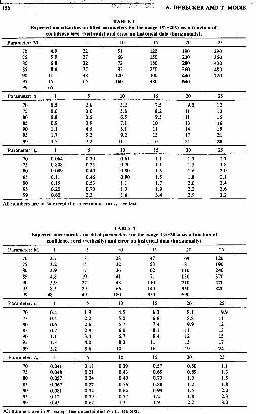
TABLE 1 Expected uncertainties on fitted parameters for the range 1%-20% as a function of
confidence level (vertically) and error on historical data (horizontally).
Parameter: M 1 5 10 15 20 25
70 4.9 22 51 120 190 290 75 5.9 27 60 150 230 360 80 6.8 32 72 180 280 430 85 8.6 37 92 250 360 480 90 11 48 120 300 440 720 95 15 65 160 480 640 99 65
Parameter: a 1 5 10 15 20 25
70 0.5 2.6 5.2 7.5 9.0 12 75 0.6 3.0 5.8 8.2 11 13 80 0.8 3.5 6.5 9.5 11 15 85 0.9 3.9 7.1 10 13 16 90 1.1 4.5 8.1 11 14 19 95 1.7 5.2 9.2 13 17 21 99 3.5 7.2 11 16 21 28
Parameter: I , 1 5 10 15 20 25
70 0.064 0.30 0.61 1.1 1.3 1.7 75 0.808 0.35 0.70 1.1 1.5 1.8 80 0.089 0.40 0.80 1.3 1.6 2.0 85 0.11 0.46 0.90 1.5 1.8 2.1 90 0.15 0.53 1.1 1.7 2.0 2.4 95 0.20 0.70 1.3 1.9 2.2 2.6 99 0.60 2.3 1.6 3.4 2.9 3.2
All numbers are in Vo except the uncertainties on 1,; see text.
TABLE 2 Expected uncertainties on fitted parameters for the range 1%-30% as a function of
confidence level (vertically) and error on historical data (horizontally).
Parameter: M 1 5 10 15 20 25
70 2.7 13 28 47 69 120 75 3.2 15 32 53 81 190 80 3.9 17 36 62 110 240 85 4.8 19 41 71 130 370 90 5.9 22 48 110 210 470 95 8.5 29 66 140 350 820 99 48 49 180 350 690
Parameter: a 1 5 10 15 20 25
70 0.4 1.9 4.5 6.3 8.1 9.9 75 0.5 2.2 5.0 6.8 8.8 11 80 0.6 2.6 5.7 7.4 9.9 12 85 0.7 2.9 6.0 8.1 11 13 90 1.1 3.4 6.7 9.4 12 15 95 1.3 4.0 8.3 11 15 17 99 3.2 5.6 10 16 19 24
Parameter: f , 1 5 10 15 20 25
70 0.041 0.18 0.39 0.57 0.80 1.1 75 0.048 0.21 0.43 0.65 0.89 1.3 80 0.057 0.24 0.49 0.73 1 .o 1.5 85 0.067 0.27 0.56 0.88 1.2 1.8 90 0.081 0.32 0.64 0.99 1.5 2.0 95 0.12 0.39 0.17 1.2 1.8 2.3 99 0.45 0.62 1.3 1.9 2.2 3.0
All numherc are in Qln exrent the iincennintiec on t.: see text.
L DETERMINATION OF THE UNCERTAINTIES IN S-CURVE LOGISTIC FITS 157
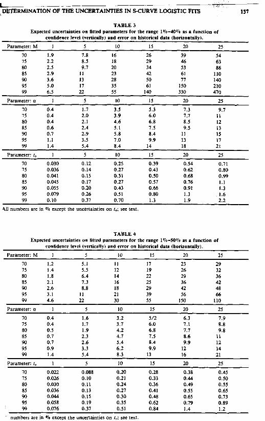
TABLE 3 Expected uncertainties on fitted parameters for the range 1%-40% as a function of
confidence level (vertically) and error on historical data (horizontally).
Parameter: M 1 5 10 15 20 25 70 1.9 7.8 16 26 39 54 75 2.2 8.5 18 29 46 63 80 2.5 9.7 20 34 53 86 85 2.9 1 1 23 42 61 110 90 3.6 13 28 50 77 140 95 5.0 17 35 61 150 210 99 6.5 22 55 140 330 470
Parameter: a 1 5 10 I5 20 25 ~
70 0.4 1.7 3.5 5.3 7.3 9.7 75 0.4 2.0 3.9 6.0 7.7 11 80 0.4 2.1 4.6 6.8 8.5 12 85 0.6 2.4 5.1 7.5 9.5 13 9o 0.7 2.9 5.8 8.4 11 15 95 1.1 3.5 7 .O 9.9 13 17 99 1.4 5.4 8.4 14 18 21
Parameter: I, I 5 10 IS 20 25 70 0.030 0.12 0.25 0.39 0.54 0.71 75 0.036 0.14 0.27 0.43 0.62 0.80 80 0.041 0.15 0.31 0.50 0.68 0.99 85 0.045 0.17 0.27 0.57 0.76 1.1 90 0.05s 0.20 0.43 0.66 0.91 1.3 95 0.079 0.26 0.5 1 0.80 1.3 1.6 99 0.10 0.37 0.70 1.3 1.9 2.2
411 numbers are in qo except the uncertainties on to; see text.
TABLE 4 Expected uncertainties on fitted parameters for the range 1%-50% as a function of
confidence level (vertically) and error on historical data (horizontally).
Parameter: M 1 5 10 15 20 25 ~ ~~
70 1.2 5.1 1 1 17 23 29 75 1.4 5.5 12 19 26 32 80 1.8 6.4 14 22 29 36 85 2.1 7.3 16 25 36 42 9o 2.6 8.8 I8 29 42 48 95 3.1 11 21 39 56 66 99 4.6 22 30 55 150 110
Parameter: a 1 5 10 15 20 25 70 0.4 1.6 3.2 5/2 6.3 7.9 75 0.4 1.7 3.7 6.0 7.1 8.8 80 0.5 1.9 4.2 6.8 7.7 9.8 85 0.7 2.3 4.7 7.5 8.6 1 1 90 0.7 2.6 5.4 8.4 9.9 12 95 0.9 3.3 6.2 9.9 12 14 99 1.4 5.4 8.3 13 16 21
Parameter: I, 1 5 10 I5 20 25 ~~~ ~
70 0.022 0.088 0.20 0.28 0.38 0.45 75 0.026 0.10 0.21 0.33 0.44 0.50 80 0.030 0.11 0.24 0.36 0.49 0.55 85 0.036 0.13 0.27 0.41 0.55 0.65 90 0.044 0.15 0.30 0.48 0.65 0.73 95 0.058 0.19 0.35 0.62 0.79 0.89 99 0.076 0.37 0.51 0.84 1.4 1.2
1 numbers are in Yo except the uncertainties on to: see text.
_______ R AND T. MQDIS
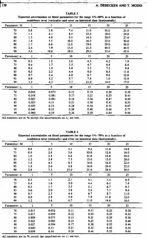
TABLE 5 Expected uncertainties on fitted parameters for the range 1%-60% as a function of
confidence level (vertically) and error on historical data (horizontally).
Parameter: M 1 5 10 15 20 25
70 0.8 3.8 7.4 11.0 16.0 21.0 75 1.1 4.1 8.1 13.0 18.0 24.0 80 1.3 4.8 9.1 14.0 20.0 27.0 85 1.4 5.5 10.0 16.0 23 .O 30.0 90 1.7 6.6 12.0 19.0 29.0 36.0 95 2.4 7.9 15.0 21 .o 44.0 44.0 99 3.3 10.0 19.0 29.0 52.0 65 .O
~~ ~~ ~ ~
Parameter: a 1 5 10 15 20 25
70 0.3 1.5 3.0 4.3 6.2 7.9 75 0.4 1.7 3.5 4.7 6.8 8.8 80 0.4 1.9 3.8 5.2 7.5 9.8 85 0.5 2.2 4.4 6.0 8.6 11.0 90 0.7 2.4 4.8 6.7 9.6 12.0 95 0.9 3.2 5.7 7.9 1 .o 13.0 99 1.2 4.3 7.7 11.0 14.0 17.0
Parameter: 1, 1 5 10 15 20 25
70 0.016 0.072 0.15 0.19 0.29 0.39 75 0.018 0.081 0.17 0.21 0.33 0.45 80 0.022 0.091 0.18 0.26 0.37 0.49 85 0.025 0.11 0.21 0.30 0.41 0.55 90 0.029 0.13 0.24 0.34 0.51 0.67 95 0.040 0.15 0.28 0.40 0.66 0.77 99 0.060 0.19 0.36 0.50 0.84 0.96
~ ~ ~ ~~
All numbers are in 070 except the uncertainties on 1.; see text.
TABLE 6 Expected uncertainties on fitted parameters for the range 1%-70070 as a function of
confidence level (vertically) and error on historical data (horizontally).
Parameter: M 1 5 10 15 20 25 ~ ~
70 0.8 75 0.9 80 1 .o 85 1.2 90 1.5 95 1.9 99 2.8
~
2.5 2.8 3.4 3.8 4.3 5.6 7.5
5.1 5.6 6.6 7.5 8.5 9.8
15.0
~~
9.2 11.0 14.0 10.0 12.0 16.0 11.0 13.0 18.0 13.0 15.0 20.0 14.0 16.0 22.0 16.0 20.0 25.0 21 .o 28.0 30.0
Parameter: a 1 5 10 15 20 25
70 0.3 1.5 2.7 4.1 5.4 6.9 75 0.4 1.6 3.0 4.4 6.1 7.6 80 0.5 1.7 3.3 5.1 6.7 8.5 85 0.6 2.0 3.8 5.8 7.7 9.6 90 0.7 2.3 4.4 6.7 8.7 11.0 95 0.9 2.8 5.0 7.9 11.0 12.0 99 1.2 3.6 6.7 11.0 14.0 16.0
Parameter: t. 1 5 10 15 20 25
70 0.015 0.052 0.11 0.17 0.22 0.28 75 0.017 0.059 0.12 0.19 0.25 0.32 80 0.030 0.073 0.13 0.21 0.29 0.36 85 0.023 0.084 0.15 0.25 0.31 0.40 90 0.021 0.094 0.17 0.38 0.35 0.44 95 0.040 0.11 0.21 0.32 0.42 0.50 99 0.058 0.16 0.28 0.46 0.53 0.66
All numbers are in 070 excent the uncertainties on L: see text.
_ _ _ v
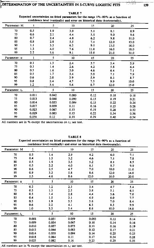
DETERMINATION OF THE UNCERTAINTIES IN S-CURVE LOGISTIC FITS 159 t- TABLE 7
Expected uncertainties on fitted parameters for the range 1Vo-8OVo as a function of confidence level (vertically) and error on historical data (horizontally).
70 0.5 1.9 3.9 5.1 8.1 8.9 75 0.6 2.1 4.4 5.5 9.0 9.6 80 0.7 2.4 4.8 6.2 9.8 11.0 85 0.8 2.8 5.5 7.1 12.0 13.0 90 1.1 3.3 6.3 9.1 13.0 16.0 95 1.3 4.0 7.6 11.0 16.0 18.0 99 2.2 5.6 9.1 15.0 21 .o 31.0
Parameter: a 1 5 10 15 20 25 70 0.3 1.3 2.4 3.7 5.4 5.9 7s 0.3 1.4 2.6 4.2 5.8 6.4 80 0.5 1.6 3 .O 4.6 6.4 7.1 85 0.5 1.7 3.4 5.0 7.1 7.9 90 0.6 2.0 3.9 5.9 8.3 8.7 95 0.8 2.4 4.7 7.5 9.9 10.0 99 1.2 3.4 2.6 8.7 12.0 15.0
Parameter: ro 1 5 10 15 20 25 70 0.01 1 0.042 0.080 0.12 0.18 0.18 75 0.013 0.048 0.090 0.13 0.19 0.21 80 0.014 0.053 0.099 0.15 0.22 0.24 85 0.017 0.059 0.11 0.16 0.25 0.28 90 0.023 0.067 0.13 0.19 0.28 0.32 95 0.029 0.083 0.15 0.22 0.34 0.36 99 0.056 0.12 0.19 0.29 0.40 0.54
All numbers are in Vo except the uncertainties on r,; see text.
TABLE 8 Expected uncertainties on fitted parameters for the range 1Vo-90Vo as a function of
confidence level (verticallv) and error on historical data (horizontallvL
Parameter: M 1 5 10 15 20 25 70 0.3 1.4 2.9 4.2 6.0 7.1 75 0.4 1.5 3.2 4.6 7.1 7.8 80 0.5 1.9 3.5 5.2 8.1 8.5 85 0.5 2.2 4.0 6.1 8.7 9.9 90 0.6 2.5 4.7 7.0 10.0 11.0 95 0.9 3.2 5.8 8.6 12.0 14.0 99 1.5 4.6 8.6 12.0 16.0 20.0
Parameter: a 1 5 10 15 20 25 70 0.2 1.2 2.3 3.4 4.7 5.4 75 0.3 1.3 2.5 3.8 5.1 6.1 80 0.3 1.4 2.8 4.4 5.6 7.0 85 0.4 1.5 3.1 4.9 6.0 7.7 90 0.5 1.9 3.5 5.6 7.0 8.4 95 0.6 2.2 4.1 6.3 8.3 9.9 99 1 .o 3.3 5.4 8.6 10.0 14.0
Parameter: r. 1 5 10 15 20 25 70 0.008 0.03 1 0.059 0.093 0.12 0.14 75 0.009 0.034 0.067 0.10 0.14 0.16 80 0.010 0.037 0.073 0.11 0.16 0.19 85 0.013 0.044 0.083 0.12 0.17 0.21 90 0.014 0.050 0.094 0.14 0.20 0.23 9s 0.018 0.064 0.11 0.17 0.24 0.28 99 0.02s 0.082 0.16 0.23 0.29 0.35
All numbers are in Vo exceut the uncertainties on 1.: see text.
I - 160 A. DEBECKERAND T. MODIS
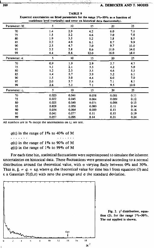
TABLE 9 Expected uncertainties on fitted parameters for the range 1%-99% as a function of
confidence level (vertically) and error on historical data (horizontally).
Parameter: M 5 10 15 20 25
70 1.4 2.9 4.2 6.0 7.1 75 1.5 3.2 4.6 7.0 7.8 80 1.9 3.5 5.2 7.8 8.5 85 2.2 4.0 6.1 8.7 9.9 90 2.5 4.7 7.0 9.7 11.0 95 3.2 5.8 8.6 11.0 14.0 99 4.4 8.6 12.0 16.0 18.0
Parameter: a 5 10 15 20 25
70 0.9 1.9 2.9 3.7 4.7 15 1.1 2.1 3.3 4.2 5 .O 80 1.2 2.3 3.5 4.6 5.5 85 1.4 2.7 3.9 5.2 6.1 90 1.5 3.0 4.4 6.0 7.0 95 2.0 3.7 5.4 7.1 8.1 99 2.6 5.1 7.1 9.5 10.0
Parameter: I, 5 I0 15 20 25
70 0.020 0.041 0.058 0.081 0.11 75 0.022 0.045 0.064 0.089 0.12 80 0.025 0.049 0.071 0.098 0.13 85 0.028 0.058 0.080 0.11 0.14 90 0.034 0.064 0.089 0.13 0.16 95 0.041 0.077 0.11 0.15 0.19 99 0.057 0.096 0.14 0.21 0.24
All numbers are in To except the uncertainties on 1,; see text.
q(ti) in the range of 1% to 40% of M
q(ti) in the range of 1% to 90% of M q(ti) in the range of 1% to 99% of M
For each time bin, statistical fluctuations were superimposed to simulate the inherent uncertainties on historical data. These fluctuations were generated according to a normal distribution around the theoretical value, with a varying flatly between 0% and 30%. That is, g, = qi + Eqi where q, the theoretical value for time bin i from equation (3) and E a Gaussian X(0,o) with zero the average and a the standard deviation.
. . . . . . . . . . . . . .
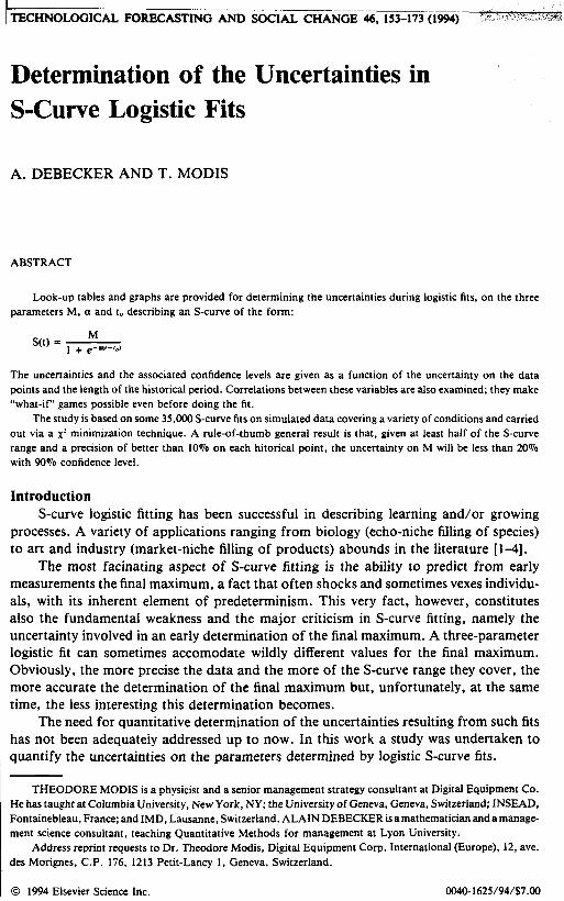
Fig. 2. x2 distribution, equa- tion (2). for the range 1%-50%. The cut applied is shown.
L DETERMINATION OF THE UNCERTAINTIES IN S-CURVE LOGISTIC FITS
___~__ 161
wed Ian = I . O U 4 incan - 1.048
- 11.5 u.11 v . : 1 . v v .
i
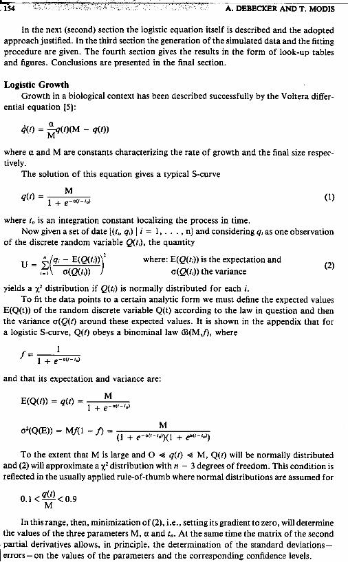
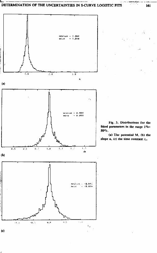
Fig. 3. Distributions for the fitled parameters in the range 1%- 50%.
(a) The potential M, (b) the slope a, (c) the time constant r,,.
3 _ - _ L _ L - ~
562 A. DEBECKER AND T. MODIS
M
1 . 5
1 . o
0 . 5
I 1 I I 1 I I 5 % 10% IS% 2 0 % 2 5 %
The life cycle curves thus obtained were subsequently integrated, producing the S-curve sections to be fitted. In this way we ensured that the statistically independent errors introduced on each time bin would be correctly accounted for in the cumulated S-curve representation.
A total of 33,693 different sections of S-curves were generated in this manner, evenly spread among the nine different time span ranges. The fits that followed were carried out by minimizing the xz of equation (2). A function minimization software package called MINUIT and developed at CERN [6] was used, providing values for M, a and to for each case. In addition the xz per degree of freedom was obtained.
Results A typical X2-distribution is shown in Figure 2, for the range 1 %-SO%. The few very
high values of xz on the tail are attributed to limitations of the function minimization software package for rare configurations of data points. A cut was applied, eliminating fits with very large x2 and reducing the data sample by less than 1 Vo. The results presented below were minimally affected by this cut.
The parameters M, a and to recovered through the fits show no systematic deviation from the true values used in generating the data. Figure 3 shows typical distributions for the parameters of the range 1 %-5O%. Even though a long tail on the M distribution biases the mean toward somewhat higher values, the median, which is more relevant in the determination of the confidence level, was found to be bias-free in all cases. Conse- quently, no systematic corrections are necessary to the fitted values.
For each range-nine in total-we present in tables I to IX the expected error on each of the parameters M, a and to as a function of the confidence level and statistical ' error of the data points. The expected error (EE) for a given parameter is defined as half I the confidence interval, i.e.,
k G I N A T I O N OF THE UNCERTAINTIES IN S-CURVE LOGISTIC FITS I63
4
1 . 1
1 . 0
0.9
1 1 I 1 1
5 : 10: 15: 20: 1 5
0.5
0.0
- 0 . 5
- 1 . 0
59. 10% 159. 20% 2 5 %
Error on d a t a
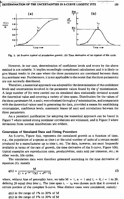
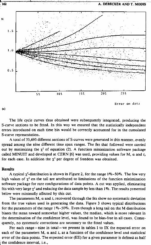
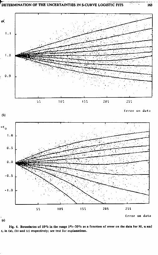
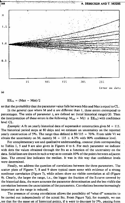
Fig. 4. Boundaries of 10% in the range 1%-20% as a function of error on the data for M, a and to in (a), (b) and (c) respectively: see text for explanations.
M I
EEcL = (Max - Min)/2
so that the probability that the parameter value falls between Min and Max is equal to CL. In the general case where M and a are different than 1, these errors correspond to
percentages. The units of parameter to are defined as: (total historical range)/20. Then the interpretation of these errors is the following: Mred = M( 1 f EEcL) with confidence level CL.
Example: A fit on yearly historical data of supertanker construction gives M = 115. The historical period stops at 80 ships and we estimate an uncertainty on the reported yearly construction of 5%. The range thus defined is 80/115 = 70%. From table VI we obtain the uncertainty on M, namely M = 115 f 4.3% with 90% confidence level.
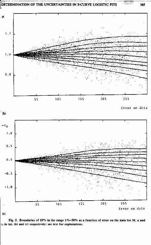
For complementary use and qualitative understanding, contour plots corresponding to Tables 1, 5 and 9 are also given in Figures 4 to 6 . For each parameter we indicate with dots the values obtained through the fits as a function of the uncertainty on the data. Solid lines are drawn in such a way as to contain 10% of the points between adjacent lines. The central line indicates the median. It was in this way that confidence levels were determined.
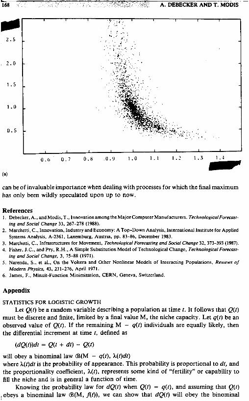
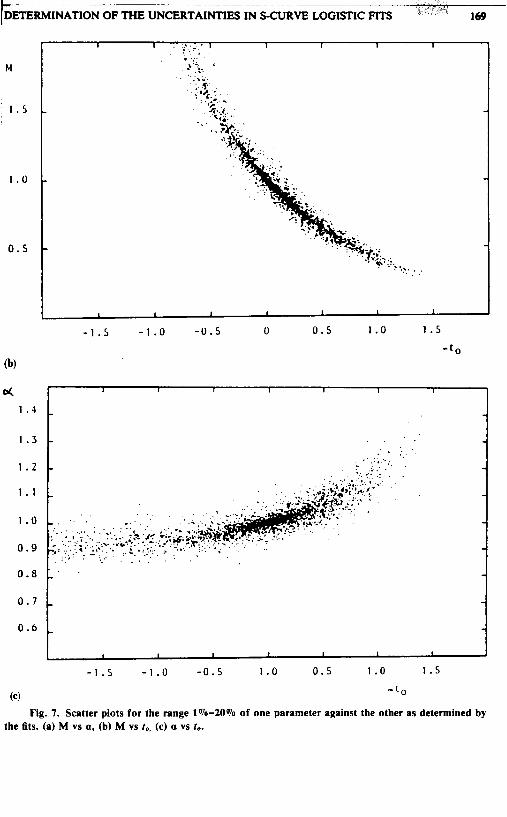
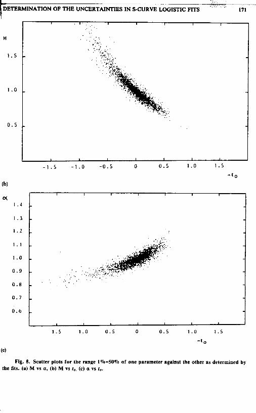
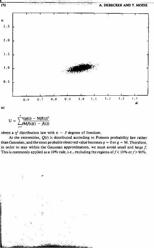
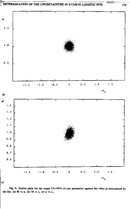
Finally, we address the question of correlations between the three parameters. The scatter plots of Figures 7, 8 and 9 show typical cases some with evidence of a strong nonlinear correlation (Figure 7), while others show no visible correlation at all (Figure 9). Clearly, the larger the range, i.e., the bigger the fraction of the S-curve covered by the historical data, the more accurate the parameter determination and the less visible the correlation between the uncertainties of the parameters. Correlations become increasingly important as the range is reduced.
The presence of strong correlations allows the possibility of "what-if" scenarios to be carried out independently of the actual fits. From Figure 7(a), for example, we can
I see that for the same set of historical Doints. if a were to decrease bv 5%. Dassine from
___ - _ _ 165
) * I F & I N A T I O N OF THE UNCERTAINTIES IN S-CURVE LOGISTIC FITS
oc I I 1 I I
1 . 1
1 . o
0.9
(b)
-f0
1 .o
0 . 5
0.0
-0.5
- 1 . 0
I
. .
I 1 1 1 I I 5: 10% 15: 20% 2 5 %
Erro r on d a t a
I I I 1 1
5% 10% 15: 2 0 % 2 5 % Error on data
(4 Fig. 5. Boundaries of 10% in the range 1%-50% as a function of error on the data for M, a and
to in (a), (b) and (c) respectively; see text for explanations.
b- 3. DEBECKER AND T. M<JIJIs ~
1 . o
51 101 I S ? 20% 25 5
Error 011 J i l t 3
(4
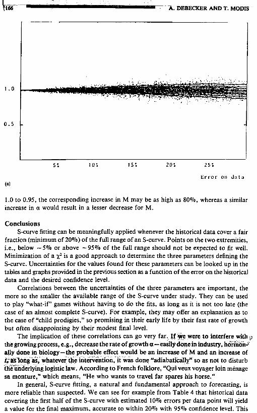
1.0 to 0.95. the corresponding increase in M may be as high as 8O%, whereas a similar increase in a would result in a lesser decrease for M.
Conclusions S-curve fitting can be meaningfully applied whenever the historical data cover a fair
fraction (minimum of 20%) of the full range of an S-curve. Points on the two extremities, i.e., below -5% or above -95% of the full range should not be expected to fit well, Minimization of a x’ is a good approach to determine the three parameters defining the S-curve. Uncertainties for the values found for these parameters can be looked up in the tables and graphs provided in the previous section as a function of the error on the historical data and the desired confidence level.
Correlations between the uncertainties of the three parameters are important, the more so the smaller the available range of the S-curve under study. They can be used to play “what-if’ games without having to do the fits, as long as it is not too late (the case of an almost complete S-curve). For example, they may offer an explanation as to the case of “child prodigies,” so promising in their early life by their fast rate of growth but often disappointing by their modest final level.
The implication of these correlations can go very far. the growing process, e.g., decrease the rate of growth a-ea
e effect would be an increase of M and an increase of tion,-it was done “adiabatidly” so as not to disturb
theunderlying logistic law. According to French folklore, “Qui veux voyager loin menage sa monture,” which means, “He who wants to travel far spares his horse.”
In general, S-curve fitting, a natural and fundamental approach to forecasting, is more reliable than suspected. We can see for example from Table 4 that historical data covering the first half of the S-curve with estimated 10% errors per data point will yield a value for the final maximum. accurate to within 20% with 95% confidence level. This
ETERMINATION OF THE UNCERTAINTIES IN S-CURVE LOGISTIC FITS 167
1 . 1
1 . o
0 . 9
- t o
1 . o
0.5
0.0
-0.5
- 1 . o
(4
I I
1 I 1 1 I
5 % 10% 1 5 % 2 0 % 2 5 %
Error on d a t a
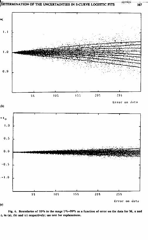
Fig. 6. Boundaries of 10% in the range 1%-99% as a function of error on the data for M, a and to in (a), (b) and (c) respectively; see text for explanations.
l e 3 * 0 . 6 0.7 0.8 0.9 1 . 0 1 . 1 1 . 2
(a)
can be of invaluable importance when dealing with processes for which the final maximum has only been wildly speculated upon up to now.
References 1. Debecker, A., and Modis, T., Innovation among the Major Computer Manufacturers. TechnologicalForecast-
2. Marchetti, C., Innovation, Industry and Economy: A Top-Down Analysis, International Institute for Applied
3. Marchetti, C., Infrastructures for Movement, Technological Forecaring and Social Change 32.373-393 (1987). 4. Fisher, J.C., and Pry, R.H., A Simple Substitution Model of Technological Change, TechnologicalForecast-
5 . Narenda. S . , et al., On the Voltera and Other Nonlinear Models of Interacting Populations, Reviews of
6. James, F., Minuit-Function Minimization, CERN, Geneva, Switzerland.
ing and Social Change 33, 267-278 (1988).
Systems Analysis, A-2361, Laxemburg, Austria, pp. 83-86, December 1983.
ing and Social Change, 3, 75-88 (1971).
Modern Physics, 43. 231-276, April 1971.
Appendix
STATISTICS FOR LOGISTIC GROWTH Let Q(t) be a random variable describing a population at time t. It follows that Q ( f )
must be discrete and finite, limited by a final value M, the niche capacity. Let q(t) be an observed value of Q(t). If the remaining M - q(t) individuals are equally likely, then the differential increment at time 1, defined as
(dQ(f))dt = Q(t + dt) - Q(0 will obey a binominal law @(M - q(t), h(t)dt) where h(r)dr is the probability of appearance. This probability is proportional to dt, and the proportionality coefficient, h(t), represents some kind of “fertility” or capability to fill the niche and is in general a function of time.
Knowing the probability law for dQ(f) when Q(t) = q(t), and assuming that Q(t) lobeys a binominal law @(M, At)), we can show that dQ(t) will obey the binominal
2 s, [DETERMINATION OF THE UNCERTAINTIES IN S-CURVE LOGISTIC FITS 169
M
1 . 5 L
1 . 0
0.5
(b)
o( 1 . 4
1 . 3
1 . z
1 . 1
1 . o
0 . 9
0 . 8
0.7
0.6
( 4
*... . .
1 I I 1 1 1 1
- 1 . 5 - 1 . 0 - 0 . 5 0 0 . 5 1 . o 1 . 5
- t o
1 I I I 1 I , - 1 . 5 - 1 . 0 - 0 . 5 1.0 0 . 5 1 . o 1 . 5
- t o
Fig. 7. Scatter plots for the range 1%-20% of one parameter against the other as determined by the fits. (a) M vs a, (b) M vs 1.. (c) a vs to.
ECKER AND T. MODIS
I I I I I I I I I
. .
- .. .
r -
CI
2 . 5
2 . 0
1 . s
1 .o
0 . 5
I I 1 1 I 1 I I 1 J 0.b 0 . 7 0.8 0.9 1 . 0 1 . 1 1 . 2 1 . 3 1 . 3
4
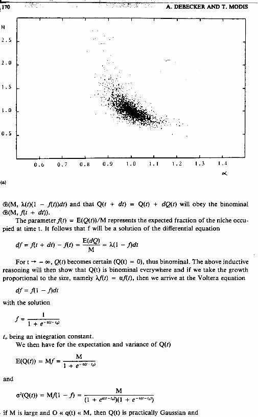
@(M, k(t)(l - fi t))dt) and that Q(t + dt) = Q(t) + dQ(r) will obey the binominal @(M,fit + dr)).
The parameterfit) = E(Q(t))/M represents the expected fraction of the niche occu- pied at time t. It follows that f will be a solution of the differential equation
df = f i t + dt) - At) = - E(dQ) - - li(i - n d t M
Fort + - 03, Q(t) becomes certain (Q(t) = 0), thus binominal. The above inductive reasoning will then show that Q(t) is binominal everywhere and if we take the growth proportional to the size, namely kAf) = Mt). then we arrive at the Voltera equation
df = f i l - ndt
with the solution
1 f = 1 + e-a(r-r,,)
to being an integration constant. We then have for the expectation and variance of Q(t)
and
. if M is large and 0 (( q(t) M, then Q(t) is practically Gaussian and
- DETERMINATION OF THE UNCERTAINTIES IN SCURVE LOGISTIC FITS . . 171
M
1 . 5
1 .o
0 . 5
- 1 . 5 - 1 . 0 - 0 . 5 0 0 . 5 1 . o 1 . 5
- t o
1 . 4
1 . 3
1 . 2
1 . 1
1 . o
0 . 9
0.8
0 . 7
0.6
1 . 5 1 .o 0 . 5 0 0 . 5 1 . o 1 . 5
- t o
(4 Fig. 8. Scatter plots for the range 1%-50% of one parameter against the other as determined by
the fits. (a) M vs a, (b) M vs ro, (c) a vs f,.
M 2.5
2 . 0
1 . 5
1 . 0
0.5
n u = c ( d t i ) - Mf(t3 l2 Mf(t i ) ( l - Ari))
i = I
obeys a x2 distribution law with n - 3 degrees of freedom. At the extremities, Q(t) is distributed according to Poisson probability law rather
than Gaussian, and the most probable observed value becomes q = 0 or q = M. Therefore, in order to stay within the Gaussian approximation, we must avoid small and large f. This is commonly applied as a 10% rule, i.e., excluding the regions off < 10% or f > 90%.
1 I I I I 1 I 1 1
-
- ,e+; .. . . ':
._:. . . .. * ..:: -
* I . : . . , L
-
1 I 1 1 I I 1 1 1
/ P
_ . I DETERMINATION OF THE UNCERTAINTIES IN S-CURVE LOGISTIC FITS * 173
1 I I I I 1 I
-
-
-
1 I I I 1 I I
M
1 . 5
1 .o
0.5
(b)
d
.. . ... .
. . . . . . I
- 1 . 5 - 1 . 0 - 0 . 5 0 0 . 5 1 .o 1 . 5
- t o
I I I I 1 I I I
1 - l . s - 1 . 0 -0.5 0 0.5 1 .o 1 . 5
- t o (4
Fig. 9. Scatter plots for the range 1%-99% of one parameter against the other as determined by the fits. (a) M vs a, (b) M vs to. (c) a vs to.