Embed Size (px)
Citation preview
Safety IDEA Program
Determination of Longitudinal Stress in Rails
Final Report for
Safety IDEA Project 15
Prepared by:
Stefan Hurlebaus
Texas Transportation Institute
College Station, Texas
July 2011
i
INNOVATIONS DESERVING EXPLORATORY ANALYSIS (IDEA)
PROGRAMS MANAGED BY THE TRANSPORTATION RESEARCH BOARD
This Safety IDEA project was funded by the Safety IDEA Program, which focuses on
innovative approaches for improving railroad safety and intercity bus and truck safety.
The Safety IDEA Program is funded by the Federal Motor Carrier Safety Administration
(FMCSA) and the Federal Railroad Administration (FRA) of the U.S. Department of
Transportation. Any opinions, findings, conclusions, or recommendations expressed in
this publication are those of the authors and do not necessarily reflect the views of the
sponsors of the Safety IDEA program.
The Safety IDEA Program is one of three IDEA programs managed by TRB. The other
two IDEA programs are listed below.
The Transit IDEA Program, which supports development and testing of innovative
concepts and methods for advancing transit practice, is funded by the Federal Transit
Administration (FTA) as part of the Transit Cooperative Research Program (TCRP).
The NCHRP Highway IDEA Program, which focuses on advances in the design,
construction, and maintenance of highway systems, is funded as part of the National
Cooperative Highway Research Program (NCHRP).
Management of the IDEA programs is coordinated to promote the development and
testing of innovative concepts, methods, and technologies for these areas of surface
transportation.
For information on the IDEA programs, look on the Internet at www.trb.org/idea, or
contact the IDEA programs office by telephone at (202) 334-3310.
IDEA Programs
Transportation Research Board
500 Fifth Street, NW
Washington, DC 20001
The project that is the subject of this contractor-authored report was a part of the Innovations
Deserving Exploratory Analysis (IDEA) Programs, which are managed by the Transportation
Research Board (TRB) with the approval of the Governing Board of the National Research
Council. The members of the oversight committee that monitored the project and reviewed the
report were chosen for their special competencies and with regard for appropriate balance. The
views expressed in this report are those of the contractor who conducted the investigation
documented in this report and do not necessarily reflect those of the Transportation Research
Board, the National Research Council, or the sponsors of the IDEA Programs. This document
has not been edited by TRB.
The Transportation Research Board of the National Academies, the National Research Council,
and the organizations that sponsor the IDEA Programs do not endorse products or
manufacturers. Trade or manufacturers' names appear herein solely because they are considered
essential to the object of the investigation.
Determination of Longitudinal Stress in Rails
Final Report
Safety IDEA Project 15
Prepared for
Safety IDEA Program
Transportation Research Board
National Research Council
Prepared by
Stefan Hurlebaus
Texas Transportation Institute
College Station, Texas
July 2011

ii
SAFETY IDEA PROGRAM COMMITTEE CHAIR ROBERT E. GALLAMORE
The Gallamore Group, LLC
MEMBERS STEPHEN A. KEPPLER
Commercial Vehicle Safety Alliance
HENRY M. LEES, JR.
Burlington Northern Santa Fe Railway (BNSF)
TOM MOORE
National Private Truck Council
DONALD A. OSTERBERG
Schneider National, Inc.
STEPHEN M. POPKIN
Volpe National Transportation Systems Center
CONRAD J. RUPPERT, JR,
National Railroad Passenger Corporation (Amtrak)
FMCSA LIAISON ALBERT ALVAREZ
Federal Motor Carrier Safety Administration
FRA LIAISON KEVIN KESLER
Federal Railroad Administration
TRB LIAISON RICHARD PAIN
Transportation Research Board
IDEA PROGRAMS STAFF STEPHEN R. GODWIN, Director for Studies and Special
Programs
JON M. WILLIAMS, Program Director, IDEA and Synthesis
Studies
HARVEY BERLIN, Senior Program Officer
DEMISHA WILLIAMS, Senior Program Assistant
EXPERT REVIEW PANEL
DAVID READ, Transportation Technology Center Inc.
DR. GARY FRY, Texas Transportation Institute
DR. LAURENCE JACOBS, Georgia Institute of Technology
iii
CONTENTS
LIST OF FIGURES AND TABLES . . . . . . . . . . . . . . . . . . . . . . . . . . . . . . . . . . . v
ACKNOWLEDGEMENTS . . . . . . . . . . . . . . . . . . . . . . . . . . . . . . . . . . . . . . . . . . . vii
ABSTRACT . . . . . . . . . . . . . . . . . . . . . . . . . . . . . . . . . . . . . . . . . . . . . . . . . . . . . . viii
EXECUTIVE SUMMARY . . . . . . . . . . . . . . . . . . . . . . . . . . . . . . . . . . . . . . . . . . 1
CHAPTER 1 Background . . . . . . . . . . . . . . . . . . . . . . . . . . . . . . . . . . . . . . . . . . . 3
Introduction . . . . . . . . . . . . . . . . . . . . . . . . . . . . . . . . . . . . . . . . . . . . . . . . . 3
Methods of Residual Stress Measurements . . . . . . . . . . . . . . . . . . . . . . . . . 4
Acoustoelastic Effect. . . . . . . . . . . . . . . . . . . . . . . . . . . . . . . . . . . . . . . . . . . 6
CHAPTER 2 Research Approach . . . . . . . . . . . . . . . . . . . . . . . . . . . . . . . . . . . . . 8
CHAPTER 3 Analytical Model of Elastic Waves . . . . . . . . . . . . . . . . . . . . . . . . . 10
Wave Propagation. . . . . . . . . . . . . . . . . . . . . . . . . . . . . . . . . . . . . . . . . . . . . . 10
Rayleigh Wave . . . . . . . . . . . . . . . . . . . . . . . . . . . . . . . . . . . . . . . . . . . . . . . . 12
Lamb Waves . . . . . . . . . . . . . . . . . . . . . . . . . . . . . . . . . . . . . . . . . . . . . . . . . . 14
States of a Solid Body . . . . . . . . . . . . . . . . . . . . . . . . . . . . . . . . . . . . . . . . . . 17
Third-Order Elastic (TOE) Constant . . . . . . . . . . . . . . . . . . . . . . . . . . . . . . . 18
CHAPTER 4 Findings and Applications . . . . . . . . . . . . . . . . . . . . . . . . . . . . . . . . 19
Equation of Motion for a Pre-stressed Body . . . . . . . . . . . . . . . . . . . . . . . . . 19
Rayleigh Waves in Pre-stressed Body . . . . . . . . . . . . . . . . . . . . . . . . . . . . . . 20
Algorithm for Numerical Simulation . . . . . . . . . . . . . . . . . . . . . . . . . . . . . . . 22
Relative Change of Rayleigh Waves on Residual Stress . . . . . . . . . . . . . . . . 23
Sensitivity Analysis . . . . . . . . . . . . . . . . . . . . . . . . . . . . . . . . . . . . . . . . . . . . 25
Rayleigh Wave Polarization . . . . . . . . . . . . . . . . . . . . . . . . . . . . . . . . . . . . . 27
Frequency Range . . . . . . . . . . . . . . . . . . . . . . . . . . . . . . . . . . . . . . . . . . . . . . 27
iv
CHAPTER 5 Experimental Setup and Results . . . . . . . . . . . . . . . . . . . . . . . . . . . . 32
Generation of Rayleigh Waves Using the Wedge Technique . . . . . . . . . . . . . 32
Experimental Setup . . . . . . . . . . . . . . . . . . . . . . . . . . . . . . . . . . . . . . . . . . . . . 34
Experimental Procedure . . . . . . . . . . . . . . . . . . . . . . . . . . . . . . . . . . . . . . . . . 35
Experimental Results in Unstressed Rail Steel . . . . . . . . . . . . . . . . . . . . . . . . 36
Experimental Results in Stressed Rail Steel . . . . . . . . . . . . . . . . . . . . . . . . . . 40
CHAPTER 6 Conclusions . . . . . . . . . . . . . . . . . . . . . . . . . . . . . . . . . . . . . . . . . . . . . 43
REFERENCES . . . . . . . . . . . . . . . . . . . . . . . . . . . . . . . . . . . . . . . . . . . . . . . . . . . . . 45
INVESTIGATOR PROFILE . . . . . . . . . . . . . . . . . . . . . . . . . . . . . . . . . . . . . . . . . . 48
v
LIST OF FIGURES AND TABLES
Page
Figure 1. Buckling of Rails (http://nisee.berkeley.edu) . . . . . . . . . . . . . . . . . . . . . . . . . 3
Figure 2. Rail Neutral Temperature . . . . . . . . . . . . . . . . . . . . . . . . . . . . . . . . . . . . . . . . 5
Figure 3. VERSE equipment (http://www.railway-technology.com). . . . . . . . . . . . . . . 5
Figure 4. Change of Rayleigh wave polarization under applied stress . . . . . . . . . . . . . 7
Figure 5. Coordinate system . . . . . . . . . . . . . . . . . . . . . . . . . . . . . . . . . . . . . . . . . . . . . 11
Figure 6. Trajectory plot for various depths (Junge, 2003) . . . . . . . . . . . . . . . . . . . . . . 14
Figure 7. Symmetric and antisymmetric components of the 1 3,u u displacements
(Hurlebaus, 2005) . . . . . . . . . . . . . . . . . . . . . . . . . . . . . . . . . . . . . . . . . . . . . 16
Figure 8. Theoretical dispersion curves calculated from Rayleigh-Lamb frequency
equations (Hurlebaus, 2005) . . . . . . . . . . . . . . . . . . . . . . . . . . . . . . . . . . . . . 16
Figure 9. Coordinate system of natural, initial, and final states of a body (Junge,
2003) . . . . . . . . . . . . . . . . . . . . . . . . . . . . . . . . . . . . . . . . . . . . . . . . . . . . . . . 18
Figure 10. The change in wave speed and the change in Rayleigh wave polarization on
residual stress for rail steel . . . . . . . . . . . . . . . . . . . . . . . . . . . . . . . . . . . . . 24
Figure 11. The change in wave speed and the change in Rayleigh wave polarization
against uncertainties . . . . . . . . . . . . . . . . . . . . . . . . . . . . . . . . . . . . . . . . . . . 26
Figure 12. Trajectory plot of particle motion for unstressed and stressed rail steel . . . 27
Figure 13. Rail steel dispersion . . . . . . . . . . . . . . . . . . . . . . . . . . . . . . . . . . . . . . . . . . . 28
Figure 14. Normalized beat length /L h vs. frequency thickness fh with
h = 17 mm . . . . . . . . . . . . . . . . . . . . . . . . . . . . . . . . . . . . . . . . . . . . . . . . . . 29
Figure 15. Experimental setup for finding frequency range effects . . . . . . . . . . . . . . . 30
Figure 16. Out-of-plane displacement amplitude vs. distance from transducer with
200 kHz excitation (top) and 1 MHz excitation (bottom) . . . . . . . . . . . . . . 31
Figure 17. Wedge transducer . . . . . . . . . . . . . . . . . . . . . . . . . . . . . . . . . . . . . . . . . . . . 32
Figure 18. Wedge transducer (Junge, 2005) . . . . . . . . . . . . . . . . . . . . . . . . . . . . . . . . . 33
Figure 19. Experimental setup using transducer. . . . . . . . . . . . . . . . . . . . . . . . . . . . . . 34
Figure 20. Sketch of out-of-plane (left) and off-angle (right) measurement . . . . . . . . 36
vi
Figure 21. Raw data in time domain . . . . . . . . . . . . . . . . . . . . . . . . . . . . . . . . . . . . . . . 37
Figure 22. In-plane and out-of-plane displacements in time domain . . . . . . . . . . . . . . 38
Figure 23. Polarization of Rayleigh wave . . . . . . . . . . . . . . . . . . . . . . . . . . . . . . . . . . . 39
Figure 24. Experimental setup at TTCI facilities . . . . . . . . . . . . . . . . . . . . . . . . . . . . . 40
Figure 25. Normalized polarization Vs. Normalized load (dots) with its trendline (solid
line) . . . . . . . . . . . . . . . . . . . . . . . . . . . . . . . . . . . . . . . . . . . . . . . . . . . . . . . 41
Table 1. Material properties of rail steel . . . . . . . . . . . . . . . . . . . . . . . . . . . . . . . . . . . . 23
Table 2. Variations of TOE Constants [GPa] and Proportionality Factors . . . . . . . . . 26
Table 3. Polarization values of 10 experiments with 800 kHz excitation frequency and
250 MHz sampling frequency . . . . . . . . . . . . . . . . . . . . . . . . . . . . . . . . . . . . . 39
vii
ACKNOWLEDGEMENTS
The research reported herein was performed by the Texas Transportation Institute
(TTI), College Station, and supported by the Safety Innovations Deserving Exploratory
Analysis (Safety IDEA) Program and the Transportation Technology Center, Inc. (TTCI).
The assistance and valuable input of the Safety IDEA program manager, Harvey Berlin,
and the expert review panel for this project comprised of David Read (TTCI), Dr. Gary T.
Fry (TTI), and Dr. Laurence J. Jacobs (Georgia Institute of Technology) is highly
appreciated.
viii
ABSTRACT
The objective of this project was to determine the longitudinal stress in rails, in
order to reduce rail buckling due to temperature-induced stresses. Continuous welded
rails (CWR) are typically long members which are susceptible to failure caused by
temperature changes. Such rail temperature changes can cause considerable disruption to
the rail network and, in the worst case, cause freight or passenger train derailment.
An important parameter in analysis of temperature induced stresses is the rail
neutral temperature (RNT), defined as that rail temperature at which the net longitudinal
force in the rail is zero. The objective of this project was to determine the longitudinal
stress in rails using the polarization of Rayleigh surface waves, to reduce buckling and
fracture.
This project developed a non-destructive procedure for monitoring the stress-free
temperature in rails using the acoustoelastic effect of ultrasonic waves. Acoustoelasticity
is the stress dependency of ultrasonic wave speed or polarization. Analytical models were
developed to explain the relationship between the polarization of Rayleigh waves and the
state of stress. Rayleigh waves were detected using a laser Doppler vibrometer (LDV).
Furthermore, the polarization of Rayleigh waves is considered as a measure to identify
applied stress.
1
EXECUTIVE SUMMARY
This research determined the rail neutral temperature (RNT) by using a non-
destructive and non-labor intensive measurement technique of the rail stress using the
polarization of Rayleigh waves. The relationship between the polarization of Rayleigh
waves and the state of stress can be seen by an analytical model. The numerical
simulation showed that the change of polarization of Rayleigh wave on residual stress is
one order of magnitude higher than the change of Rayleigh wave speed. Additionally, a
sensitivity analysis showed that the polarization of Rayleigh wave is more robust against
uncertainties in material properties. The results revealed that Rayleigh wave polarization
is more sensitive to longitudinal stress and more robust than the Rayleigh wave speed.
Further tasks as part of this project were done in order to implement this
technology in the field. A preliminary laboratory experiment was conducted where the
Rayleigh waves were generated in the rail using a wedge transducer. Then the
polarization of Rayleigh waves in an unstressed rail was detected using a laser Doppler
vibrometer (LDV) by measuring the out-of-plane as well as the in-plane component of
the particle velocity. The results of the numerical simulation were verified with the
preliminary experimental results. Further measurements were done in a stressed rail and
the change in polarization of the Rayleigh wave was determined using a wedge
transducer for generation and a LDV for the detection of ultrasonic waves. After a
thorough evaluation, the concept was tested at Transportation Technology Center, Inc.
(TTCI) facilities in Pueblo, CO, to transfer the developed technology to TTCI researches
and Association of American Railroads (AAR) members. The results show that the
polarization of Rayleigh wave changes with longitudinal stress. Knowing the longitudinal
stress will prevent future buckling of the rail and reduce the number of derailments and
increase railroad safety.
In a period of four years, 99 derailments occurred in the U.S resulting in about
$38 million in damages. In total, there were ten times as many incidents of rail buckling
due to temperature effects as those that resulted in derailments (Kish and Read).
2
The potential impacts of the application of this proposed technique on railroads
are reduction of maintenance costs and increased safety. The non-destructive and non-
labor intensive maintenance reduces the time needed to do inspections. The potential for
cost savings in the U.S. railroad industry is considerable. This practical method gives the
railroad industry the opportunity to check their rail lines more often and to correct the
installation of the rails at the RNT, which can reduce buckling of the rail and decrease the
number of train derailments.
3
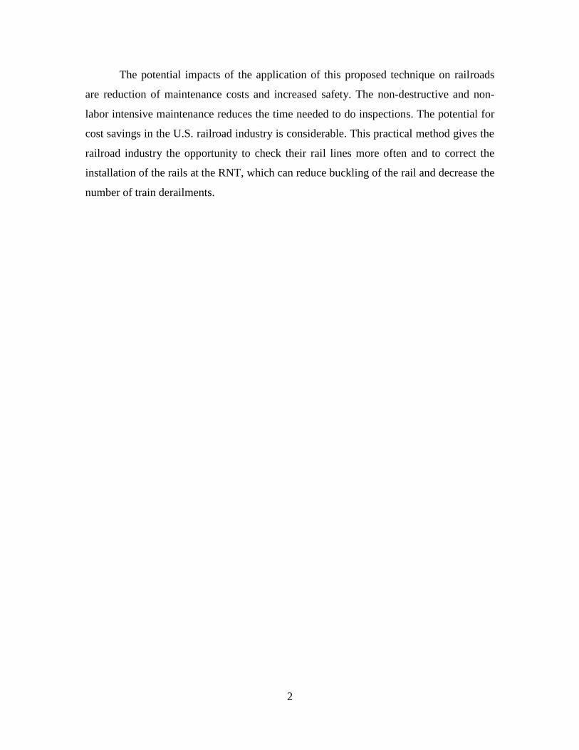
Fig. 1 – Buckling of Rails (http://nisee.berkeley.edu)
CHAPTER 1
Background
Introduction
Continuous welded rails (CWR) are rails that are welded together to become long
continuous members that are fixed at both ends. Using CWR will improve the
convenience and reduce unneeded abrasion. There are also disadvantages in using CWR.
Rail steel expands in hot weather and shrinks in cold weather, which could cause
buckling and fracturing. Due to fixed ends, rails are restrained from expanding and
shrinking. Hence, rails will experience a compressive stress in hot weather and they will
undergo a tensile stress in cold conditions. The temperature at which the rails experience
zero stress is called the rail neutral temperature (RNT). Large difference between the
RNT and the surrounding temperature can cause the rails to buckle or fracture. Fig. 1
shows how rails could buckle due to a large difference between RNT and ambient
temperature.
To prevent this problem, RNT needs to be set up to be in between the buckling
and fracturing temperature. Kish and Samavedam (2005) identified that the RNT of rail
steel could change due to several factors such as rail movement through fasteners.
Moreover, the temperature of the rail can exceed the ambient temperature by around 30oF
4
in hot weather, causing the rail steel to reach temperatures of 140oF. This results in
having a greater chance of rail buckling. For example, a CWR is installed at 90oF (RNT =
90oF). Consider that rail buckling happens at a temperature difference of 60
oF. Thus, rail
will buckle when the temperature reaches to 150oF. Due to rail movement through
fastener, RNT drops to 50oF. This change in RNT causes the rail to buckle when the
temperature reaches 100oF.
The example above shows how important it is to keep inspecting the RNT of
CWR. Installing CWR at a “safe” region between buckling and fracturing temperatures
does not guarantee that the rail will not buckle in the future. Hence, in order to prevent
the rails from buckling or fracturing, RNT needs to be identified on a timely basis.
The objective of this research is to identify the longitudinal stress by using the
polarization of Rayleigh waves in a non-destructive and non-labor intensive method. The
ultrasonic wave will be generated by a transducer, and a laser Doppler vibrometer (LDV)
is used to measure both the in-plane and out-of-plane velocity components of a Rayleigh
wave as a function of applied stress (Hurlebaus and Jacobs, 2006). Once the longitudinal
stress is identified and the ambient temperature is measured, RNT can then be calculated
by using the relation between stress, ambient temperature, and the material properties
given by
n aT TE
, (1.1)
where nT is the rail neutral temperature, aT is the ambient temperature, is the residual
stress, E is Young’s Modulus, and is the thermal coefficient. The graph of this
relation can be seen in Fig. 2. Once the RNT is determined, the conditions of the rails can
be known, and decisions can be made regarding whether re-installing the entire rail is
necessary to increase safety.
5
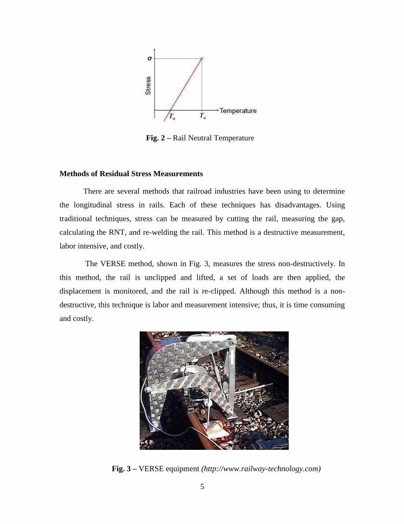
Fig. 2 – Rail Neutral Temperature
Fig. 3 – VERSE equipment (http://www.railway-technology.com)
Methods of Residual Stress Measurements
There are several methods that railroad industries have been using to determine
the longitudinal stress in rails. Each of these techniques has disadvantages. Using
traditional techniques, stress can be measured by cutting the rail, measuring the gap,
calculating the RNT, and re-welding the rail. This method is a destructive measurement,
labor intensive, and costly.
The VERSE method, shown in Fig. 3, measures the stress non-destructively. In
this method, the rail is unclipped and lifted, a set of loads are then applied, the
displacement is monitored, and the rail is re-clipped. Although this method is a non-
destructive, this technique is labor and measurement intensive; thus, it is time consuming
and costly.
6
Egle and Bray (1979) use the acoustoelastic effect on longitudinal wave speed
using contact transducers. The disadvantages of this method are that a very precise
measurement of propagation distance is needed to determine the longitudinal wave speed,
and the correlation between longitudinal wave speed and residual stress is low.
The d’Stresen technique (Read, 2007) identifies that the vibration amplitude of a
rail is proportional to the longitudinal force in the rail, but only when the rail is under
tension. Also, this technique is a contact measurement technique; thus, it cannot be
applied while trains are running. Damljanovic and Weaver (2005) investigated the
technique of measuring the stress in rails using the principle of sensitivity of bending
rigidity to stress. This technique measures the bending wave number in the rail for the
unstressed and stressed case. The drawback of this technique is that it requires a very
high precision equipment to do the experiment.
Acoustoelastic Effect
The determination of material properties such as material constants, flaw
detection, or applied stress can be obtained by various types of ultrasonic waves. Crecraft
(1962, 1967) found that acoustoelasticity or the acoustoelastic effect is a functional
technique for determining material properties. Using the correlation of the stress
dependence of wave velocities in solids, the dependency of ultrasonic waves on stress is
called the acoustoelastic effect.
Murnaghan (1951) developed a nonlinear elastic theory for isotropic materials.
This theory introduces third-order elastic (TOE) constants which help explain the
acoustoelastic effect with a theoretical model. The theory was applied by Toupin and
Berstein (1961) to an elastically deformed material to observe the propagation behavior
of acoustic waves. Pao and Garmer (1985) extended this theory to an orthotropic media.
The acoustoelastic effect is very small. Special techniques are required to measure
the stress-induced velocity changes. Crecraft (1967) uses the sing-around technique to
measure the acoustoelastic effect. This technique uses one or two transducers that are
7
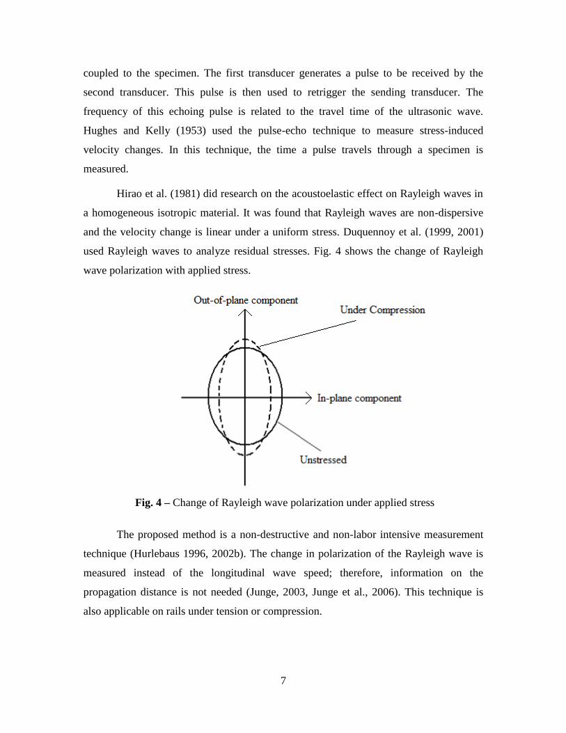
Fig. 4 – Change of Rayleigh wave polarization under applied stress
coupled to the specimen. The first transducer generates a pulse to be received by the
second transducer. This pulse is then used to retrigger the sending transducer. The
frequency of this echoing pulse is related to the travel time of the ultrasonic wave.
Hughes and Kelly (1953) used the pulse-echo technique to measure stress-induced
velocity changes. In this technique, the time a pulse travels through a specimen is
measured.
Hirao et al. (1981) did research on the acoustoelastic effect on Rayleigh waves in
a homogeneous isotropic material. It was found that Rayleigh waves are non-dispersive
and the velocity change is linear under a uniform stress. Duquennoy et al. (1999, 2001)
used Rayleigh waves to analyze residual stresses. Fig. 4 shows the change of Rayleigh
wave polarization with applied stress.
The proposed method is a non-destructive and non-labor intensive measurement
technique (Hurlebaus 1996, 2002b). The change in polarization of the Rayleigh wave is
measured instead of the longitudinal wave speed; therefore, information on the
propagation distance is not needed (Junge, 2003, Junge et al., 2006). This technique is
also applicable on rails under tension or compression.
8
CHAPTER 2
Research Approach
The following investigations were done as part of the current project:
1: Literature Review
The research team compiled a literature review to fully document the state of
practice on estimating the rail stress. The team will continue the literature review
throughout the duration of the project to identify new information and to identify possible
issues and areas of improvement.
2: Analytical Model
This task developed an analytical model that predicts the relationship between the
polarization of a Rayleigh wave and the state of stress. This relationship is used to
measure applied stress. The analytical model is based on the equations of motion for a
pre-stressed body.
3: Numerical Simulation
The numerical simulation for the problem concerning Rayleigh waves in a pre-
stressed medium was performed. First, an iterative algorithm that solves the relevant
analytical equations was developed followed by an analysis of the numerical problem.
Moreover, a sensitivity analysis was performed that investigates the influence of
uncertainties in the third order elastic constants on the wave speed and the polarization.
4: Preliminary Experiment
The purpose of this preliminary experiment was focused on how to generate
Rayleigh waves in rails using a wedge transducer. Then the polarization of Rayleigh
waves in an unstressed rail were detected using a laser Doppler vibrometer (LDV) by
measuring the out-of-plane as well as the in-plane component of the particle velocity.
5: Model Updating
Verification of the results of the numerical simulation with the preliminary
experimental results was done. This provides the opportunity to account for any
uncertainties in material properties of the rail or for any geometrical uncertainties.
9
6: Experiment
Measurements were done in TTCI facilities at Pueblo, CO. by using hydraulic
clamps to do a tension test. The experiment was done by using a wedge transducer for
Rayleigh wave generation, and the change in polarization of the Rayleigh wave between
stressed and unstressed rail steel was determined.
10
CHAPTER 3
Analytical Model of Elastic Waves
This chapter provides descriptions on the subject of wave propagation, Rayleigh
waves, states of a solid body, and third-order constant (TOE). These subjects help in
understanding the analytical model discussed in the next chapter.
Wave Propagation
The equation of motion of an elastic solid is governed by the Lame-Navier
equation given by
2
2
mn mm
n
T uf
x t
, (3.1)
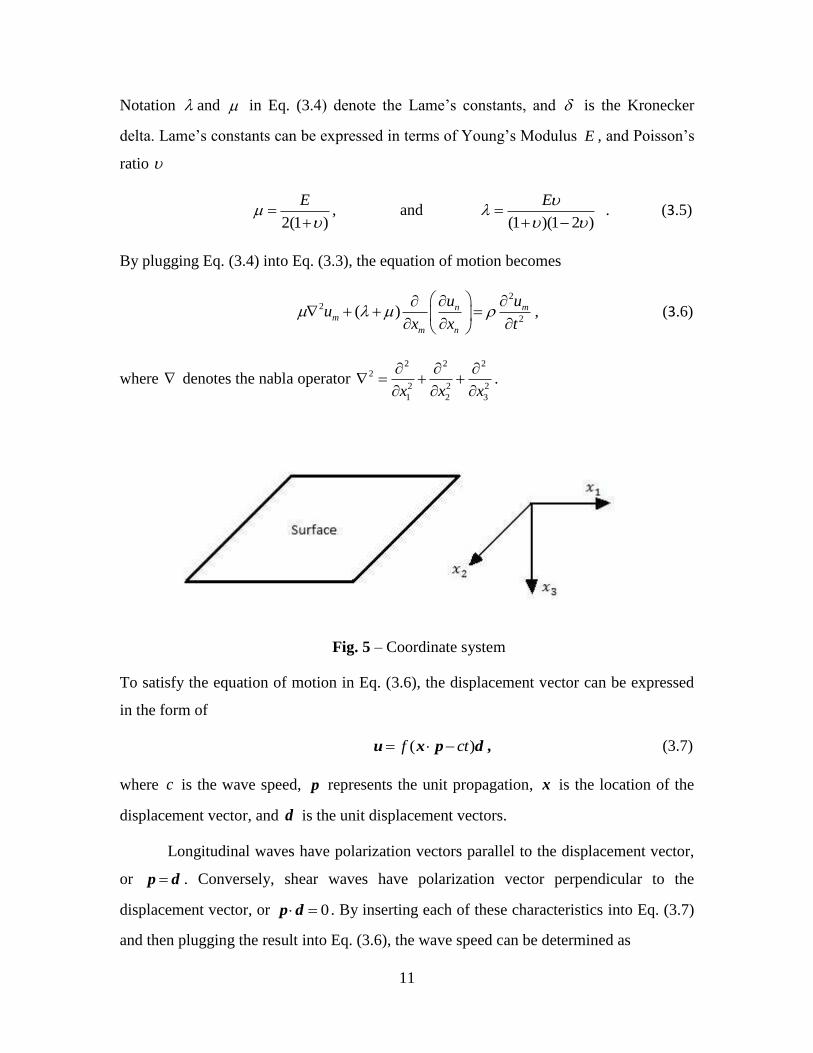
where symbolizes the density of the material, mf are the internal body forces, nx
denotes the direction in the coordinate system shown in Fig. 5, mu is the displacement in
the mx direction, and mnT denotes the stress tensor in the generalized Hooke’s Law given
as
p
mn mnpq
q
uT C
x
. (3.2)
By substituting Eq. (3.2) to Eq. (3.1) and neglecting the body forces, the equation of
motion can be written as
2 2
2
p mmnpq
n q
u uC
x x t
, (3.3)
where mnpqC is the second order stiffness tensor given by
( )mnpq mn pq mp nq mq nqC . (3.4)
11
Notation and in Eq. (3.4) denote the Lame’s constants, and is the Kronecker
delta. Lame’s constants can be expressed in terms of Young’s Modulus E , and Poisson’s
ratio
2(1 )
E
, and
(1 )(1 2 )
E
. (3.5)
By plugging Eq. (3.4) into Eq. (3.3), the equation of motion becomes
2
2
2( ) n m
m
m n
u uu
x x t
, (3.6)
where denotes the nabla operator 2 2 2
2
2 2 2
1 2 3x x x
.
Fig. 5 – Coordinate system
To satisfy the equation of motion in Eq. (3.6), the displacement vector can be expressed
in the form of
( )f ct u x p d , (3.7)
where c is the wave speed, p represents the unit propagation, x is the location of the
displacement vector, and d is the unit displacement vectors.
Longitudinal waves have polarization vectors parallel to the displacement vector,
or p d . Conversely, shear waves have polarization vector perpendicular to the
displacement vector, or 0 p d . By inserting each of these characteristics into Eq. (3.7)
and then plugging the result into Eq. (3.6), the wave speed can be determined as
12
2 2lc
, (3.8)
2
Sc
, (3.9)
where lc and Sc are the longitudinal wave speed and the shear wave speed, respectively.
Eq. (3.7) can be uncoupled in terms of longitudinal and shear waves by utilizing
the Helmholtz decomposition. The displacement in uncoupled terms can be expressed in
terms of a scalar function and a vector field ψ
u ψ . (3.10)
By substituting Eq. (3.10) back into Eq. (3.6), the uncoupled equations are
22
2 2
1
lc t
and
22
2 2
1
sc t
ψψ
. (3.11)
Rayleigh Wave
A Rayleigh wave is a non dispersive wave that propagates on the free surface of a
solid. It was first found by Lord Rayleigh in 1885 (Hurlebaus, 2002a). The particles of a
Rayleigh wave travel in a counterclockwise direction with an elliptic trajectory along the
free surface and then change to a clockwise direction as the depth increases. A Rayleigh
wave’s amplitude decays as a function of depth (coordinate 3x ), and the motion does not
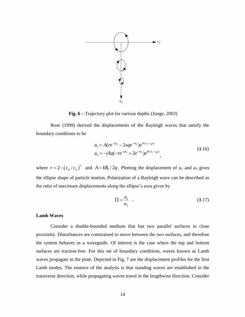
depend on the coordinate 2x . Fig. 6 shows the trajectory plot of a Rayleigh wave particle.
In Rayleigh waves, the scalar function and vector field can be assumed to be
1( )
3( )ik x ct
F x e
1( )
3( )ik x ct
G x e
ψ , (3.12)
where F and G are functions of 3x , and k is the wave number given by 2 /k .
Plugging Eq. (3.12) into Eq. (3.11) gives the surface wave motion
13
3 1( )
1
kqx ik x ctAe e
3 1( )
1
ksx ik x ctB e e
ψ , (3.13)
where 1A and 1B are arbitrary constants and
2
1 R
l
cq
c
2
1 R
s
cs
c
.
The boundary conditions require that stress is equal to zero at 3 0x . Substitution of this
boundary condition into Eq. (3.13) yields the Rayleigh characteristic equation
22 2 2
2 2 22 4 1 1 0R R R
s l s
c c c
c c c
. (3.14)
Eq. (3.14) has six roots, whose values depend only on Poisson’s ratio for a given
elastic media. Victorov (1966) showed that for arbitrary values of corresponding to
real media (0 < < 0.5), Eq. (3.14) has only one such root. An approximate expression
for the Rayleigh wave velocity Rc is given by Graff (1991)
0.87 1.12
1
R
S
c
c
. (3.15)
This propagation velocity is smaller than those of the body waves. As the velocity Rc is
independent of the wavelength, the wave propagation is non dispersive. The propagation
of a Rayleigh wave is depicted in Fig. 6. It can be shown that an arbitrary point will move
with elliptical motion as the Rayleigh wave passes by. Most of the energy in the Rayleigh
wave is present in the depth of one wavelength from the surface. Due to this skin effect,
the Rayleigh wave has great potential for detection of faults at the surface of structures.
Furthermore, the Rayleigh wave causes the most damage during an earthquake because it
carries more energy at the surface than either longitudinal or shear waves.
14
Fig. 6 – Trajectory plot for various depths (Junge, 2003)
Rose (1999) derived the displacements of the Rayleigh waves that satisfy the
boundary conditions to be
3 3 1
3 3 1
( )
1
( )
3
( 2 )
( 2 )
R
R
qx sx ik x c t
qx sx ik x c t
u A re sqe e
u iAq re e e
,
(3.16)
where 2
2 /R Sr c c and 1 / 2A kB q . Plotting the displacement of u1 and u3 gives
the ellipse shape of particle motion. Polarization of a Rayleigh wave can be described as
the ratio of maximum displacements along the ellipse’s axes given by
1
3
u
u
. (3.17)
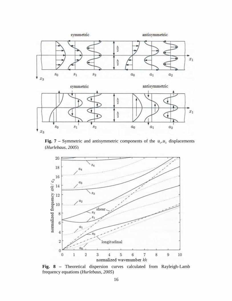
Lamb Waves
Consider a double-bounded medium that has two parallel surfaces in close
proximity. Disturbances are constrained to move between the two surfaces, and therefore
the system behaves as a waveguide. Of interest is the case where the top and bottom
surfaces are traction-free. For this set of boundary conditions, waves known as Lamb
waves propagate in the plate. Depicted in Fig. 7 are the displacement profiles for the first
Lamb modes. The essence of the analysis is that standing waves are established in the
transverse direction, while propagating waves travel in the lengthwise direction. Consider
15
a plane, harmonic Lamb wave propagating along the positive 1x -direction in a plate with
thickness h. The scalar and vector potentials can be expressed as
1( )2 2 2 2
1 3 2 3sin cosik x ct
L LC k k x C k k x e
(3.18)
1( )2 2 2 2
1 3 2 3sin cosik x ct
S SD k k x D k k x e
, (3.19)
where Lk and Sk are the wave numbers of the longitudinal and shear waves, respectively,
1C , 2C , 1D and 2D are arbitrary constant. Implementation of the boundary conditions
33 13 0 at the free surface 3 / 2x h leads, after some manipulation, to the well-
known Rayleigh-Lamb frequency equations
2 22 2 2 2 2
2 2 22 2
tanh42
(2 )tanh
2
SS L
SL
hk k
k k k k k
h k kk k
(3.20)
for the symmetric case and
2 2
2 2 2
2 2 2 2 22 2
tanh(2 )2
4tanh2
S
S
S LL
hk k
k k
h k k k k kk k
(3.21)
for the antisymmetric case. For the symmetric mode shapes, the displacement 1u is
symmetric about the axis 3 0x ; and for the antisymmetric mode shapes the
displacement 1u is antisymmetric about the axis 3 0x (Fig. 7). At a spatially-fixed plate
cross section, the amplitude of a mode shape will oscillate with angular frequency as
wavefronts travel through the cross-section with velocity c. Eq. (3.20) and Eq. (3.21) can
be expressed in terms of and c using the relationship /k c .
16
Fig. 7 – Symmetric and antisymmetric components of the 1 3,u u displacements
(Hurlebaus, 2005)
Fig. 8 – Theoretical dispersion curves calculated from Rayleigh-Lamb
frequency equations (Hurlebaus, 2005)
17
For a given frequency, these equations can be solved for the unknown velocity of
the mode in question. A plot of vs. c (or vs. k) for a particular mode is known as a
dispersion curve. Fig. 8 shows typical dispersion curves in the normalized ( , k) domain
for Lamb waves together with dispersion curves for the longitudinal and shear wave. The
symmetric Lamb modes are called 0 1 2, , ,...s s s and the antisymmetric modes are
called 0 1 2, , ,...a a a . Lamb waves are – as opposed to Rayleigh waves – dispersive,
whereby the propagation velocity of a specific Lamb mode depends upon its oscillation
frequency. For a given ( , k) combination, the mode shape can be computed using Eq.
(3.11), Eq. (3.18), and Eq. (3.19). Fig. 7 shows the in-plane and out-of-plane
displacements 1 3,u u for symmetric as well as for antisymmetric Lamb waves.
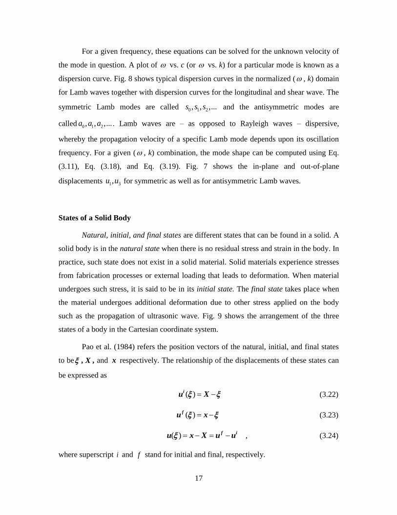
States of a Solid Body
Natural, initial, and final states are different states that can be found in a solid. A
solid body is in the natural state when there is no residual stress and strain in the body. In
practice, such state does not exist in a solid material. Solid materials experience stresses
from fabrication processes or external loading that leads to deformation. When material
undergoes such stress, it is said to be in its initial state. The final state takes place when
the material undergoes additional deformation due to other stress applied on the body
such as the propagation of ultrasonic wave. Fig. 9 shows the arrangement of the three
states of a body in the Cartesian coordinate system.
Pao et al. (1984) refers the position vectors of the natural, initial, and final states
to be , X , and x respectively. The relationship of the displacements of these states can
be expressed as
( ) iu X (3.22)
( ) fu x (3.23)
( ) f iu x X u u , (3.24)
where superscript i and f stand for initial and final, respectively.
18
Fig. 9 – Coordinate system of natural, initial, and final states of a body (Junge, 2003)
Third-Order Elastic (TOE) Constant
The existence of elastic constants is very important in determining the stress state
of the material using the ultrasonic wave method. The second order elastic constant can
be found by using the linear theory of elasticity. When there is an applied stress in the
material, the second order elastic constants cannot explain the change in ultrasonic wave
velocities. Thus, a higher order of nonlinear elasticity theory was established. This theory
introduces the second-order Lame constant and the third-order elastic constant. For
isotropic materials, the second- and third-order elastic constants can be expressed in the
forms
( )C , (3.25)
and
1 2
3
[ ( ) ( )
( )] [ ( )
( ) ( )
( )],
C
(3.26)
where 1 , 2 , and 3 are the Toupin and Bernstein (1961) notation of TOE.
19
CHAPTER 4
Findings and Applications
Equation of Motion for a Pre-stressed Body
The state of stress at a given point as a function of X is defined by the Cauchy
stress tensor, ( )it X . While the Piola-Kirchhoff stress tensor,
iT (ξ) , describes the state of
stress at the same given point in the natural configuration. Both of these tensors are
related by
1
i iJKJK
XXt T
X
ξ . (4.1)
The relation of the final state of stress of these two tensors can also be found by using the
same analogy given by
1 1
j jf f fi iij KL
K L
x xx xt T T
x x
ξ X , (4.2)
and the stress change from the initial to final state is defined by
f i
JK JK JKT T t
f iT T t . (4.3)
Given these basic explanations, Pao et al. (1984) derives the equation of motion as
2
0
2ˆ( ) (1 )i i iK
IK JL IJKL NN
J L
uut C
X X t
, (4.4)
where ˆIJKLC represents the adapted stress tensor of a pre-stressed body. Both the adapted
stress tensor and initial strain are respectively given by
1
2 2
3
ˆ ( ) [( )
( )( )] 2( )( )
2( )( )
IJKL IJ KL IK JL IL JK IJ KL
i i i
IK JL IL JK MM IJ KL KL IJ
i i i i
IK JL IL JK JK IL JL IK
C
,
(4.5)
20
and the initial strain, i
KL , is determined by
1
2 (3 2 ) 2
i i i
KL KL NN KLt t
. (4.6)
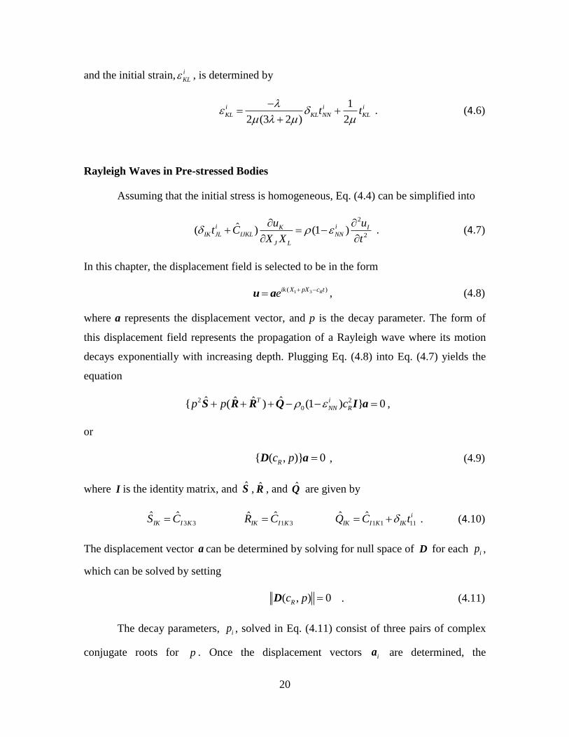
Rayleigh Waves in Pre-stressed Bodies
Assuming that the initial stress is homogeneous, Eq. (4.4) can be simplified into
2
2ˆ( ) (1 )i iK I
IK JL IJKL NN
J L
u ut C
X X t
. (4.7)
In this chapter, the displacement field is selected to be in the form
1 3( )Rik X pX c te
u a , (4.8)
where a represents the displacement vector, and p is the decay parameter. The form of
this displacement field represents the propagation of a Rayleigh wave where its motion
decays exponentially with increasing depth. Plugging Eq. (4.8) into Eq. (4.7) yields the
equation
2 2
0ˆ ˆˆ ˆ{ ( ) (1 ) } 0T i
NN Rp p c S R R Q I a ,
or
{ ( , )} 0Rc p D a , (4.9)
where I is the identity matrix, and S , R , and Q are given by
3 3ˆ ˆ
IK I KS C 1 3ˆˆ
IK I KR C 1 1 11ˆ ˆ i
IK I K IKQ C t . (4.10)
The displacement vector a can be determined by solving for null space of D for each ip ,
which can be solved by setting
( , ) 0Rc p D . (4.11)
The decay parameters, ip , solved in Eq. (4.11) consist of three pairs of complex
conjugate roots for p . Once the displacement vectors ia are determined, the
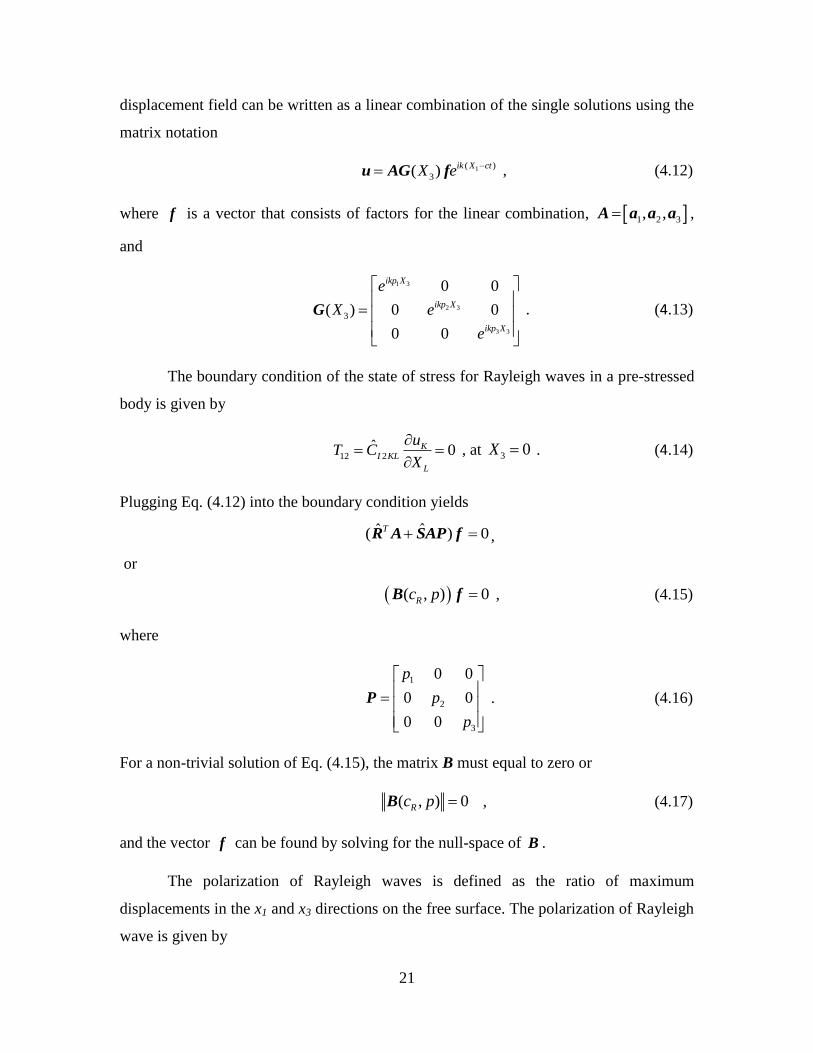
21
displacement field can be written as a linear combination of the single solutions using the
matrix notation
1( )
3( )ik X ct
X e
u AG f , (4.12)
where f is a vector that consists of factors for the linear combination, 1 2 3, ,A a a a ,
and
1 3
2 3
3 3
3
0 0
( ) 0 0
0 0
ikp X
ikp X
ikp X
e
X e
e
G . (4.13)
The boundary condition of the state of stress for Rayleigh waves in a pre-stressed
body is given by
12 2
ˆ 0KI KL
L
uT C
X
, at 3 0X . (4.14)
Plugging Eq. (4.12) into the boundary condition yields
ˆˆ( ) 0T R A SAP f ,
or
( , ) 0Rc p B f , (4.15)
where
1
2
3
0 0
0 0
0 0
p
p
p
P . (4.16)
For a non-trivial solution of Eq. (4.15), the matrix B must equal to zero or
( , ) 0Rc p B , (4.17)
and the vector f can be found by solving for the null-space of B .
The polarization of Rayleigh waves is defined as the ratio of maximum
displacements in the x1 and x3 directions on the free surface. The polarization of Rayleigh
wave is given by
22
1
2
( )
( )
Af
Af . (4.18)
Algorithm for Numerical Simulation
The numerical simulation to the problem of Rayleigh wave propagation is done
by using Matlab software. This simulation determines the changes of Rayleigh wave
speed, Rc , and polarization of the Rayleigh wave, , due to residual stresses. Junge
(2003) has arranged the iterative algorithm as follows:
1. Identify an initial Rayleigh wave speed, 0Rc . This can be done by using Eq.
(3.14). The longitudinal and shear wave speeds can be determined by using Eq.
(3.8) and Eq. (3.9). Poisson’s ratio is needed to perform this calculation, and it
can be found by
2( )
(4.19)
2. Plug in the wave speed from step 1 into Eq. (4.9) and solve for pi that makes the
determinant of D equal to zero.
3. For each value of ip , solve for the null-space, ia , in Eq. (4.9) and construct the
matrix A .
4. Use the values of p to construct the matrix P in Eq. (4.16).
5. Construct matrix B as stated in Eq. (4.15).
6. If the determinant of matrix B is not equal to zero, use another value of 0Rc and
start all over again from step 2.
7. The value of 0Rc that satisfies the boundary condition is the Rayleigh wave speed,
Rc , due to the residual stress.
8. Solve for the null-space, f , in Eq. (4.15)
9. Compute the polarization vector using Eq. (4.18)
23
Relative Change of Rayleigh Waves on Residual Stress
The relative change of the wave speed and polarization with stress are very small
in rail steel. Many publications use the relative change of wave speed instead of the
absolute value of the wave speed and polarization because of this reason. Moreover, the
acoustoelastic effect can be clearly visualized by using the relative change. The relative
change of Rayleigh wave speed is given by
0
0
R RR
R
c cc
c
, (4.20)
and the relative change of Rayleigh wave polarization is
0
0
. (4.21)
The numerical simulation in this chapter uses the properties of rail steel found by Egle
and Bray (1976) that are shown in Table 1.
ρ λ μ υ1 υ2 υ3
(kg/m3) (GPa) (GPa) (GPa) (GPa) (GPa)
7799 110.7 82.4 -96 -254 -181
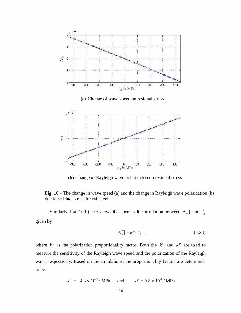
Rail steel has yield strength of 450 MPa. This simulation runs the analysis ranging
from a compressive force of -440 MPa to a tensile force of 440 MPa. Fig. 10(a) shows
the results of the simulation on the change of wave speed due to residual stress. This plot
shows that there is a linear relation between them and is given by
11
c i
Rc k t , (4.22)
where ck is a wave speed proportionality factor.
Table 1 – Material properties of rail steel
24
(a) Change of wave speed on residual stress
(b) Change of Rayleigh wave polarization on residual stress
Fig. 10 – The change in wave speed (a) and the change in Rayleigh wave polarization (b)
due to residual stress for rail steel
Similarly, Fig. 10(b) also shows that there is linear relation between and 11
it
given by
11
p ik t , (4.23)
where pk is the polarization proportionality factor. Both the ck and pk are used to
measure the sensitivity of the Rayleigh wave speed and the polarization of the Rayleigh
wave, respectively. Based on the simulations, the proportionality factors are determined
to be
ck = -4.3 x 10⁻⁷
/ MPa and pk = 9.8 x 10⁻⁶
/ MPa
25
Sensitivity Analysis
In the previous section, TOE constants are assumed to remain unchanged in the
simulation. In reality, the values of TOE constants have some uncertainties. Eagle and
Bray (1976) identified an estimated error of the TOE constants for rail steel to be about
3% - 4%. Smith et al. (1966) found the uncertainties of TOE constants for austenitic Steel
Hecla ATV to be more than 20%. As can be seen for the examples, sensitivity analysis on
the TOE constants needs to be done to discover the change of wave speed and
polarization of Rayleigh waves against uncertainties for any case. In contrast, Lame
constants can be determined precisely and, hence, can be assumed to remain constant.
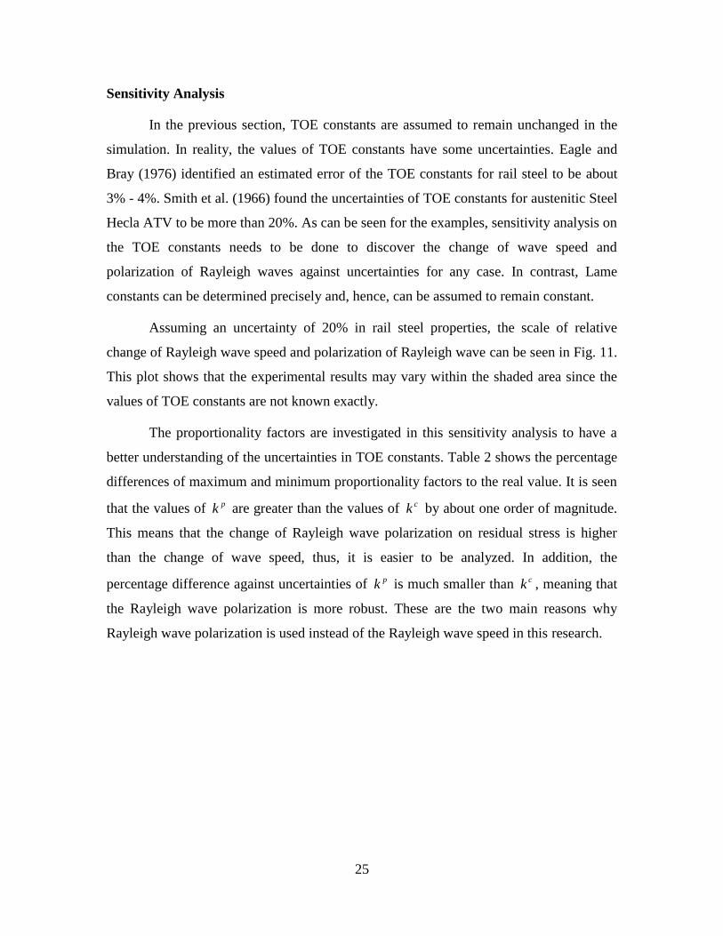
Assuming an uncertainty of 20% in rail steel properties, the scale of relative
change of Rayleigh wave speed and polarization of Rayleigh wave can be seen in Fig. 11.
This plot shows that the experimental results may vary within the shaded area since the
values of TOE constants are not known exactly.
The proportionality factors are investigated in this sensitivity analysis to have a
better understanding of the uncertainties in TOE constants. Table 2 shows the percentage
differences of maximum and minimum proportionality factors to the real value. It is seen
that the values of pk are greater than the values of ck by about one order of magnitude.
This means that the change of Rayleigh wave polarization on residual stress is higher
than the change of wave speed, thus, it is easier to be analyzed. In addition, the
percentage difference against uncertainties of pk is much smaller than ck , meaning that
the Rayleigh wave polarization is more robust. These are the two main reasons why
Rayleigh wave polarization is used instead of the Rayleigh wave speed in this research.
26
(a) Change of wave speed against uncertainties
(b) Change of polarization of Rayleigh wave against uncertainties
Fig. 11 – The change in wave speed (a) and the change in Rayleigh wave polarization (b)
against uncertainties. The changes are within the shaded area.
Table 2 - Variations of TOE Constants [GPA] and Proportionality Factors
υ1 υ2 υ3 ck % diff pk % diff
Min -115.2 -304.8 -217.2 -2.69E-06 519.65% 1.34E-05 36.78%
Avg -96 -254 -181 -4.34E-07
9.76E-06
Max -76.8 -203.2 -144.8 1.82E-06 -519.64% 6.17E-06 -36.77%
27
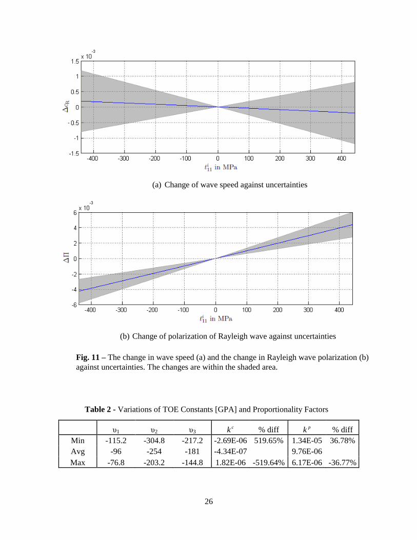
Fig. 12 – Trajectory plot of particle motion for unstressed and stressed rail
steel
Rayleigh Wave Polarization
The values of Rayleigh wave polarization are obtained by dividing the
displacements in the x1 direction by the displacements in the x3 direction. These values
can also be plotted against each other to visualize the shape of particle motion. Fig. 12
shows the change in the shape in particle motion between unstressed and stressed rail
steel.
Frequency Range
Ideally, the Rayleigh wave can only propagate along an elastic half-space. In this
research, the Rayleigh wave is generated to propagate on the web of rail steel. The web of
the rail steel itself is a plate like structure. Hence, a frequency range where the Rayleigh
wave theory can be applied needs to be determined.
This propagation of Rayleigh wave itself is a superposition of the first
antisymmetric and symmetric Lamb modes as explained by Victorov (1966). In a
previous section of this report, Lamb waves are explained in more detail.
28
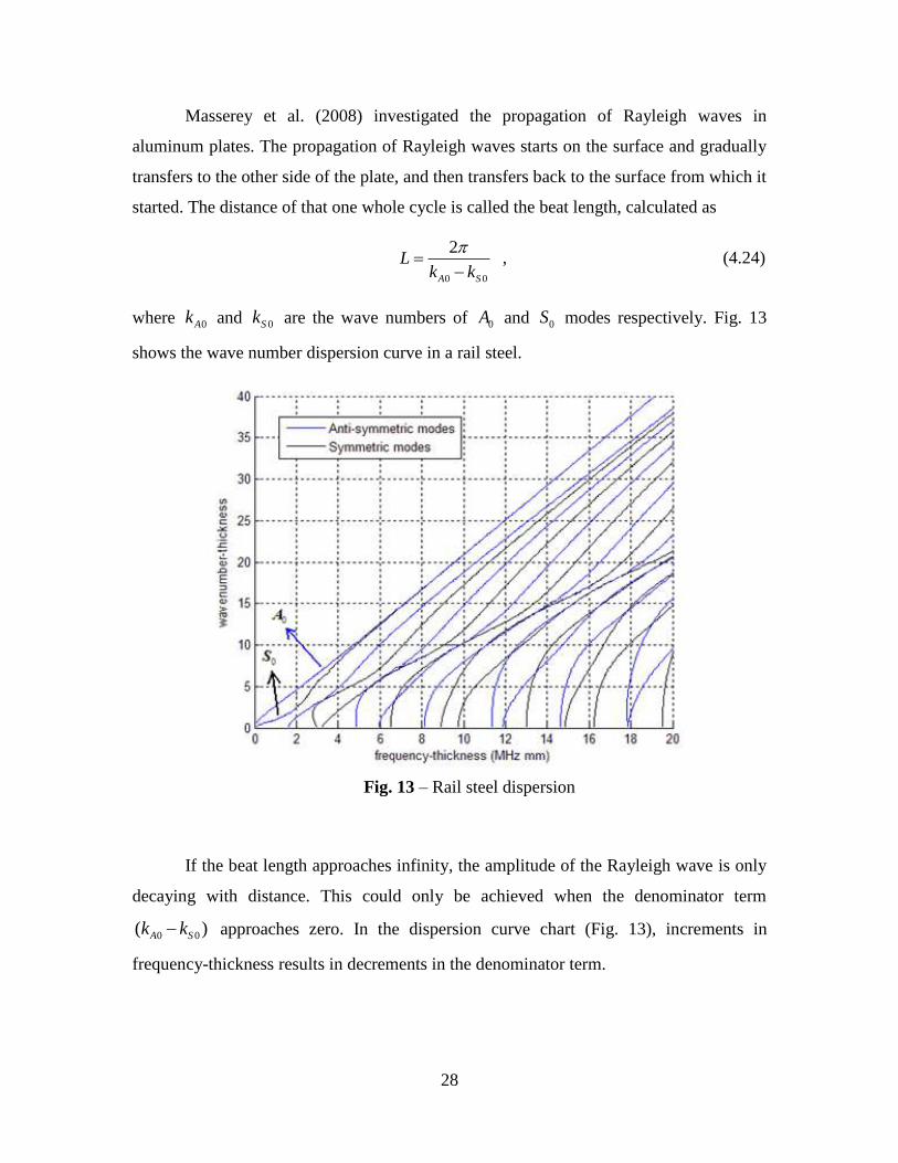
Masserey et al. (2008) investigated the propagation of Rayleigh waves in
aluminum plates. The propagation of Rayleigh waves starts on the surface and gradually
transfers to the other side of the plate, and then transfers back to the surface from which it
started. The distance of that one whole cycle is called the beat length, calculated as
0 0
2
A S
Lk k
, (4.24)
where 0Ak and 0Sk are the wave numbers of 0A and 0S modes respectively. Fig. 13
shows the wave number dispersion curve in a rail steel.
If the beat length approaches infinity, the amplitude of the Rayleigh wave is only
decaying with distance. This could only be achieved when the denominator term
0 0( )A Sk k approaches zero. In the dispersion curve chart (Fig. 13), increments in
frequency-thickness results in decrements in the denominator term.
Fig. 13 – Rail steel dispersion
curve
29
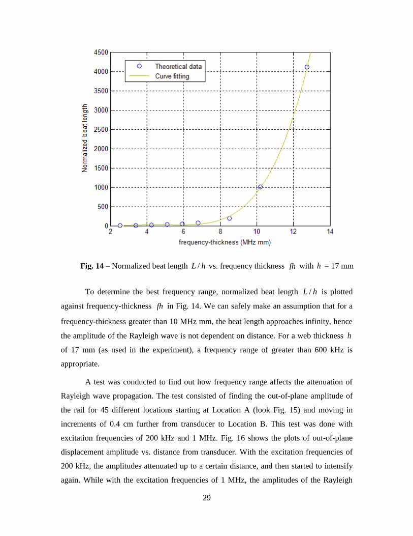
To determine the best frequency range, normalized beat length /L h is plotted
against frequency-thickness fh in Fig. 14. We can safely make an assumption that for a
frequency-thickness greater than 10 MHz mm, the beat length approaches infinity, hence
the amplitude of the Rayleigh wave is not dependent on distance. For a web thickness h
of 17 mm (as used in the experiment), a frequency range of greater than 600 kHz is
appropriate.
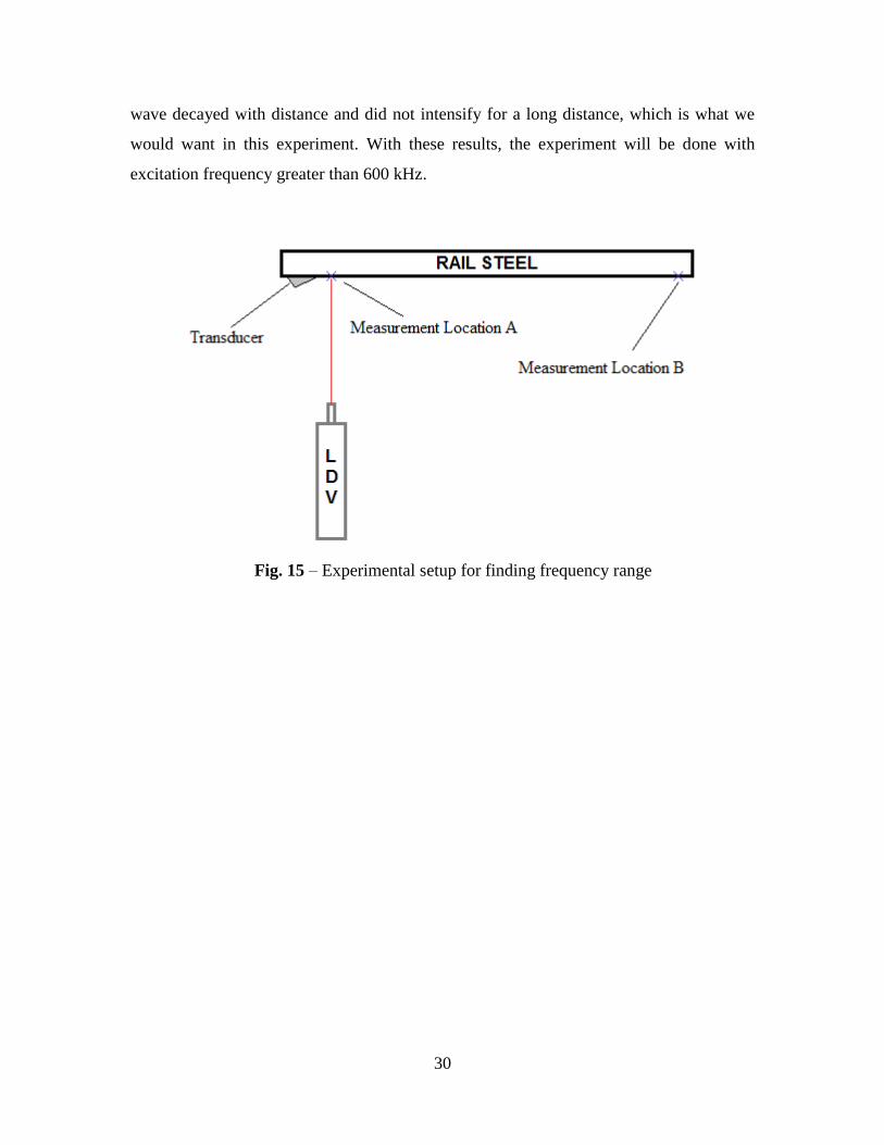
A test was conducted to find out how frequency range affects the attenuation of
Rayleigh wave propagation. The test consisted of finding the out-of-plane amplitude of
the rail for 45 different locations starting at Location A (look Fig. 15) and moving in
increments of 0.4 cm further from transducer to Location B. This test was done with
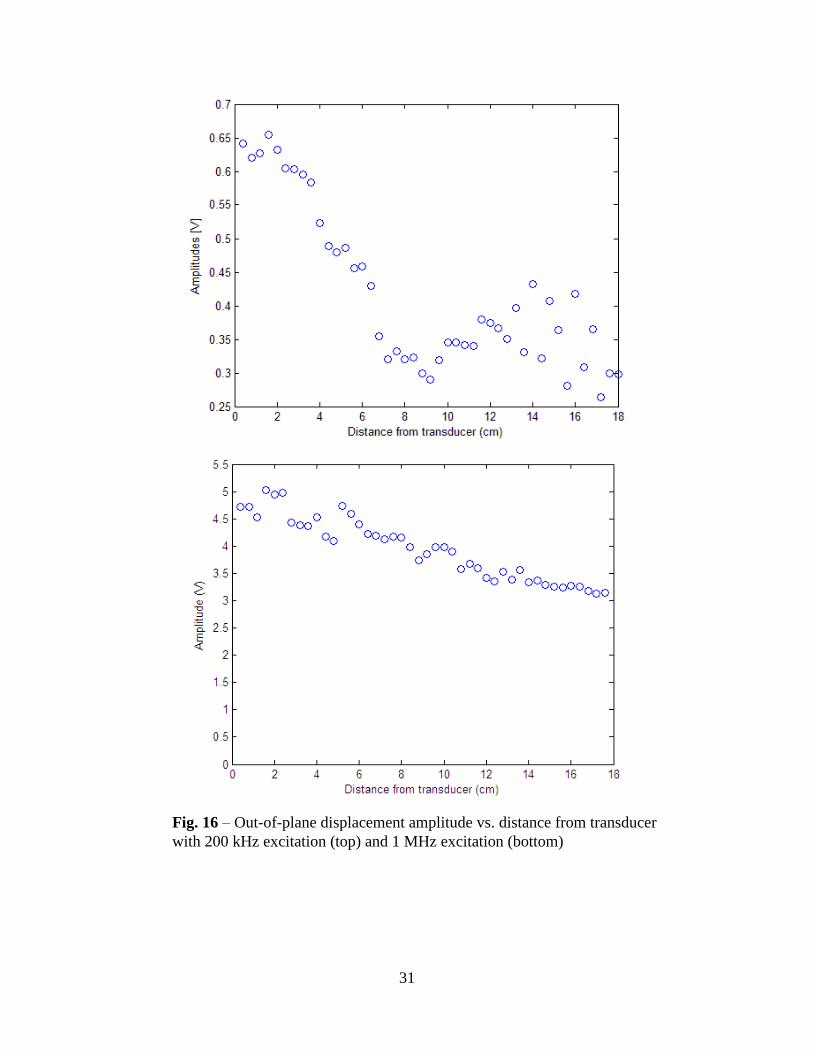
excitation frequencies of 200 kHz and 1 MHz. Fig. 16 shows the plots of out-of-plane
displacement amplitude vs. distance from transducer. With the excitation frequencies of
200 kHz, the amplitudes attenuated up to a certain distance, and then started to intensify
again. While with the excitation frequencies of 1 MHz, the amplitudes of the Rayleigh
Fig. 14 – Normalized beat length /L h vs. frequency thickness fh with h = 17 mm
30
wave decayed with distance and did not intensify for a long distance, which is what we
would want in this experiment. With these results, the experiment will be done with
excitation frequency greater than 600 kHz.
Fig. 15 – Experimental setup for finding frequency range
31
Fig. 16 – Out-of-plane displacement amplitude vs. distance from transducer
with 200 kHz excitation (top) and 1 MHz excitation (bottom)
32
Fig. 17 – Wedge transducer
CHAPTER 5
Experimental Setup and Results
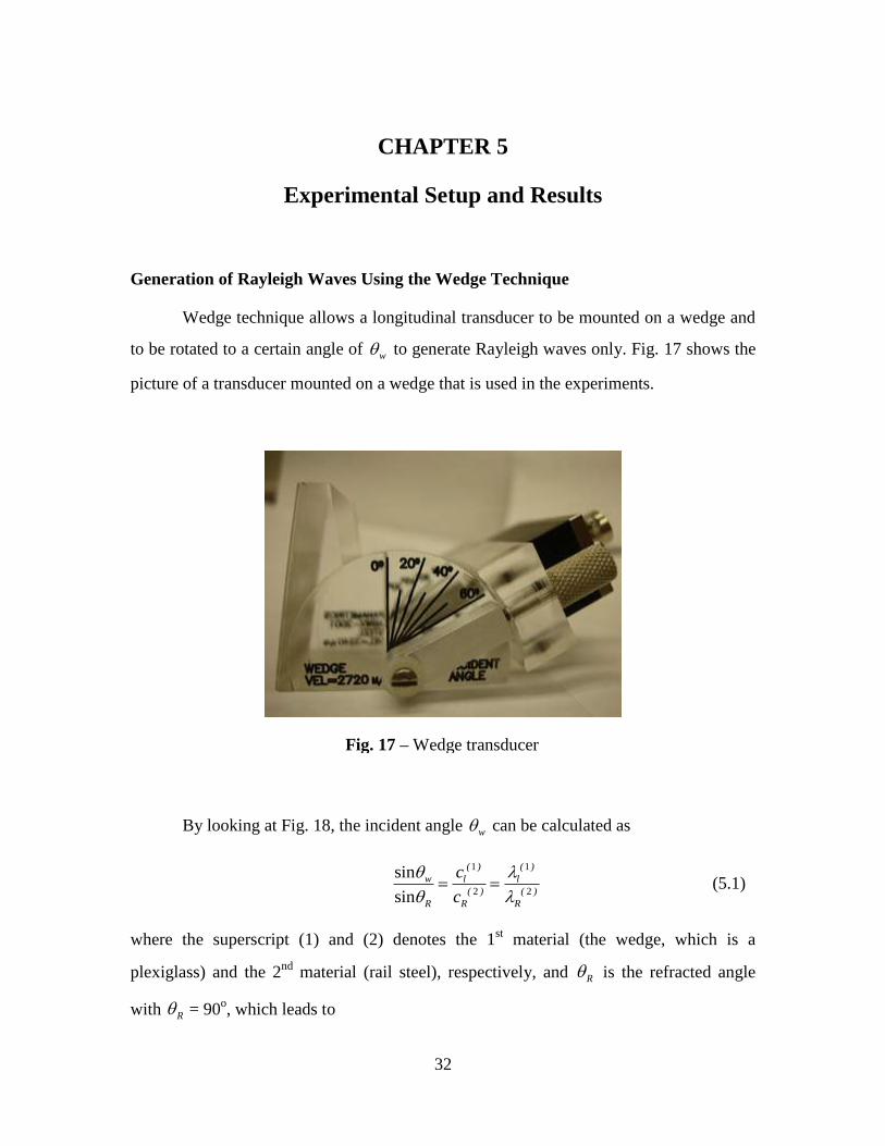
Generation of Rayleigh Waves Using the Wedge Technique
Wedge technique allows a longitudinal transducer to be mounted on a wedge and
to be rotated to a certain angle of w to generate Rayleigh waves only. Fig. 17 shows the
picture of a transducer mounted on a wedge that is used in the experiments.
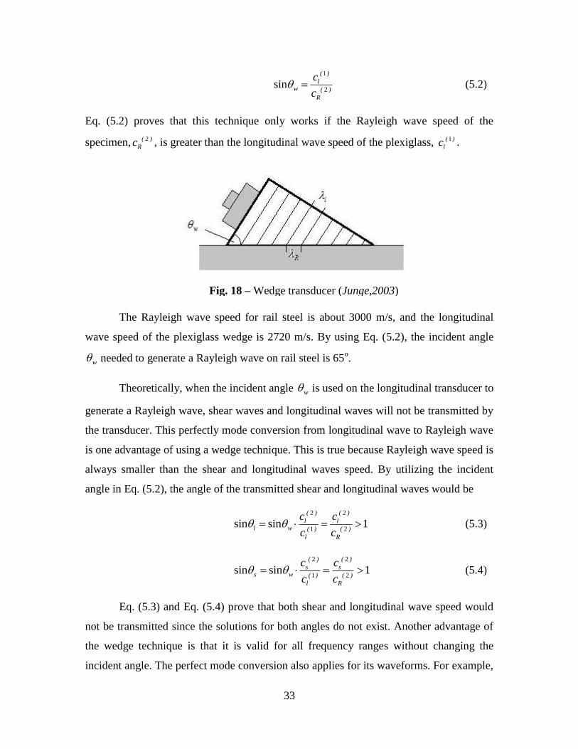
By looking at Fig. 18, the incident angle w can be calculated as
1 1
2 2
sin
sin
( ) ( )
w l l
( ) ( )
R R R
c
c
(5.1)
where the superscript (1) and (2) denotes the 1st material (the wedge, which is a
plexiglass) and the 2nd
material (rail steel), respectively, and R is the refracted angle
with R = 90o, which leads to
33
Fig. 18 – Wedge transducer (Junge,2003)
1
2sin
( )
lw ( )
R
c
c (5.2)
Eq. (5.2) proves that this technique only works if the Rayleigh wave speed of the
specimen, 2( )
Rc , is greater than the longitudinal wave speed of the plexiglass, 1( )
lc .
The Rayleigh wave speed for rail steel is about 3000 m/s, and the longitudinal
wave speed of the plexiglass wedge is 2720 m/s. By using Eq. (5.2), the incident angle
w needed to generate a Rayleigh wave on rail steel is 65o.
Theoretically, when the incident angle w is used on the longitudinal transducer to
generate a Rayleigh wave, shear waves and longitudinal waves will not be transmitted by
the transducer. This perfectly mode conversion from longitudinal wave to Rayleigh wave
is one advantage of using a wedge technique. This is true because Rayleigh wave speed is
always smaller than the shear and longitudinal waves speed. By utilizing the incident
angle in Eq. (5.2), the angle of the transmitted shear and longitudinal waves would be
2 2
1 2sin sin 1
( ) ( )
l ll w ( ) ( )
l R
c c
c c (5.3)
2 2
1 2sin sin 1
( ) ( )
s ss w ( ) ( )
l R
c c
c c (5.4)
Eq. (5.3) and Eq. (5.4) prove that both shear and longitudinal wave speed would
not be transmitted since the solutions for both angles do not exist. Another advantage of
the wedge technique is that it is valid for all frequency ranges without changing the
incident angle. The perfect mode conversion also applies for its waveforms. For example,
34
Fig. 19 – Experimental setup using transducer
a longitudinal wave with sinusoidal waveform will stay as a sinusoidal waveform when it
is mode converted to a Rayleigh wave.
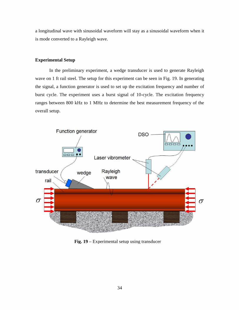
Experimental Setup
In the preliminary experiment, a wedge transducer is used to generate Rayleigh
wave on 1 ft rail steel. The setup for this experiment can be seen in Fig. 19. In generating
the signal, a function generator is used to set up the excitation frequency and number of
burst cycle. The experiment uses a burst signal of 10-cycle. The excitation frequency
ranges between 800 kHz to 1 MHz to determine the best measurement frequency of the
overall setup.
35
The transducer used in this experiment is a Centrascan series C401 from
Panametrics with a center frequency of 1 MHz. This transducer is attached to an angle
beam Panametrics wedge ABWX-2001. The transducer is set up at an incident angle w
of 65o as specified in the previous section.
The Rayleigh wave detection is done by using a laser Doppler vibrometer (LDV).
The basic concept of this vibrometer is to detect the frequency shift or phase shift of the
laser light that is reflected from a vibrating surface. This Doppler frequency (or phase)
shift is then used to determine the surface velocity of the particles. Kil et al. (1998)
explained more about LDV system in details.
A Digital Storage Oscilloscope (DSO) Tektronix TDS 3034B is used to record the
data captured by the LDV. The signals are averaged five-hundred-twelve times to
increase the signal-to-noise-ratio (SNR).
Experimental Procedure
To obtain the in-plane and out-of-plane component, measurements from two
different angles are necessary. The first measurement is done by setting the LDV
perpendicular to the rail to measure the out-of-plane velocity. The second measurement is
done under an angle of from the axis of the web of the rail. Figure 20 shows the sketch
of experimental setup for the out-of-plane measurement and the off-angle measurement.
In order to obtain the in-plane component of the measured signals the relation
sin( ) sin( )1
cos( ) cos( )sin( )
IP b a a
OP b a ba b
V V
V V
(5.5)
is used, where IPV , and OPV are the in-plane and out-of-plane velocity components,
respectively, a , and b are the angles measured from the axis of the web of the rail, and
aV , and bV are the velocity components measured under the angle of a and b ,
respectively.
The first measurement is done by setting the LDV perpendicular ( a from the axis
of the web) to the rail to measure the out-of-plane velocity. The second measurement is
36
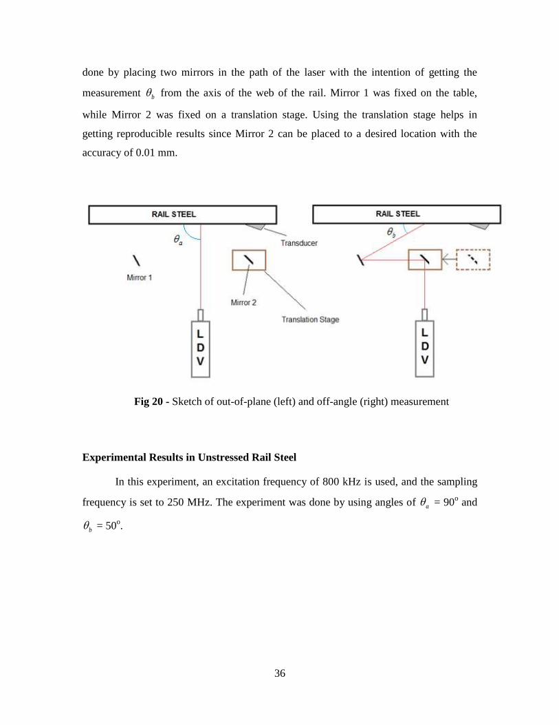
Fig 20 - Sketch of out-of-plane (left) and off-angle (right) measurement
done by placing two mirrors in the path of the laser with the intention of getting the
measurement b from the axis of the web of the rail. Mirror 1 was fixed on the table,
while Mirror 2 was fixed on a translation stage. Using the translation stage helps in
getting reproducible results since Mirror 2 can be placed to a desired location with the
accuracy of 0.01 mm.
Experimental Results in Unstressed Rail Steel
In this experiment, an excitation frequency of 800 kHz is used, and the sampling
frequency is set to 250 MHz. The experiment was done by using angles of a = 90o and
b = 50
o.
37
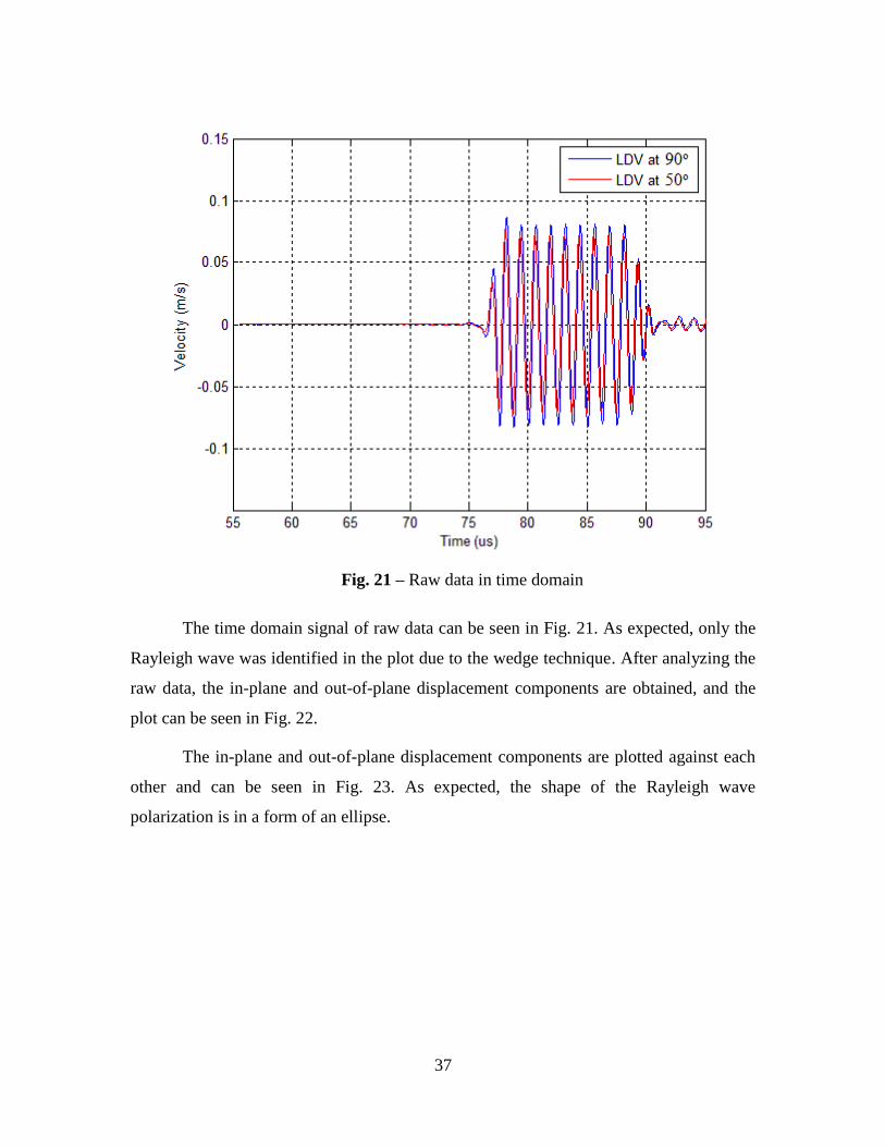
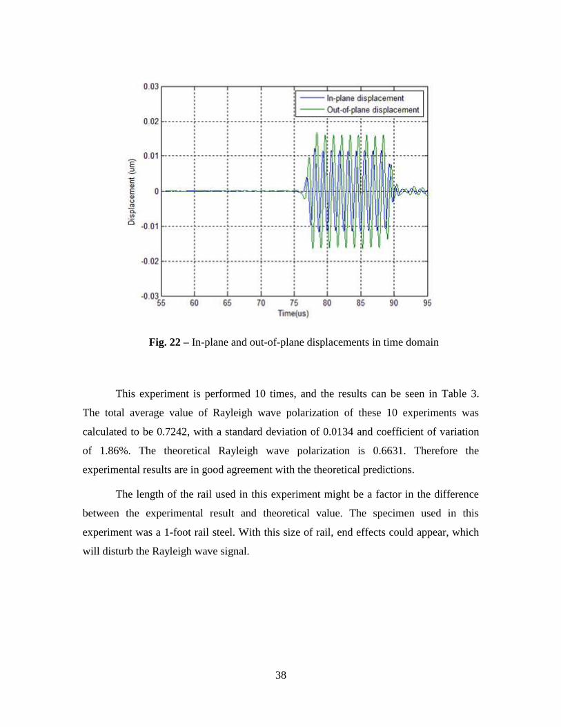
The time domain signal of raw data can be seen in Fig. 21. As expected, only the
Rayleigh wave was identified in the plot due to the wedge technique. After analyzing the
raw data, the in-plane and out-of-plane displacement components are obtained, and the
plot can be seen in Fig. 22.
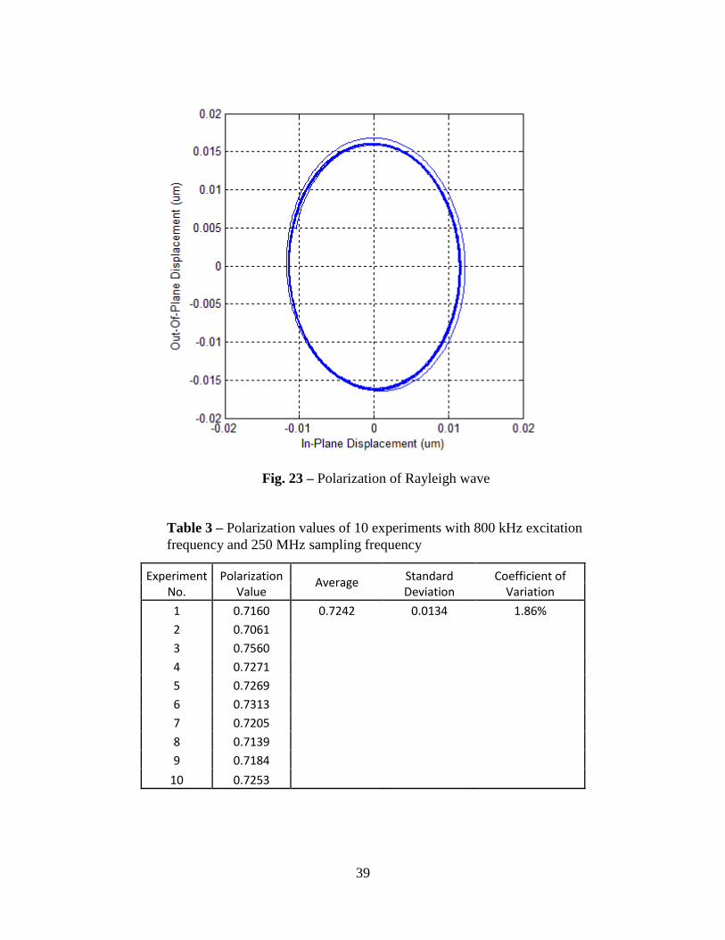
The in-plane and out-of-plane displacement components are plotted against each
other and can be seen in Fig. 23. As expected, the shape of the Rayleigh wave
polarization is in a form of an ellipse.
Fig. 21 – Raw data in time domain
38
This experiment is performed 10 times, and the results can be seen in Table 3.
The total average value of Rayleigh wave polarization of these 10 experiments was
calculated to be 0.7242, with a standard deviation of 0.0134 and coefficient of variation
of 1.86%. The theoretical Rayleigh wave polarization is 0.6631. Therefore the
experimental results are in good agreement with the theoretical predictions.
The length of the rail used in this experiment might be a factor in the difference
between the experimental result and theoretical value. The specimen used in this
experiment was a 1-foot rail steel. With this size of rail, end effects could appear, which
will disturb the Rayleigh wave signal.
Fig. 22 – In-plane and out-of-plane displacements in time domain
39
Experiment No.
Polarization Value
Average Standard Deviation
Coefficient of Variation
1 0.7160 0.7242 0.0134 1.86%
2 0.7061
3 0.7560
4 0.7271
5 0.7269
6 0.7313
7 0.7205
8 0.7139
9 0.7184
10 0.7253
Fig. 23 – Polarization of Rayleigh wave
Table 3 – Polarization values of 10 experiments with 800 kHz excitation
frequency and 250 MHz sampling frequency
40
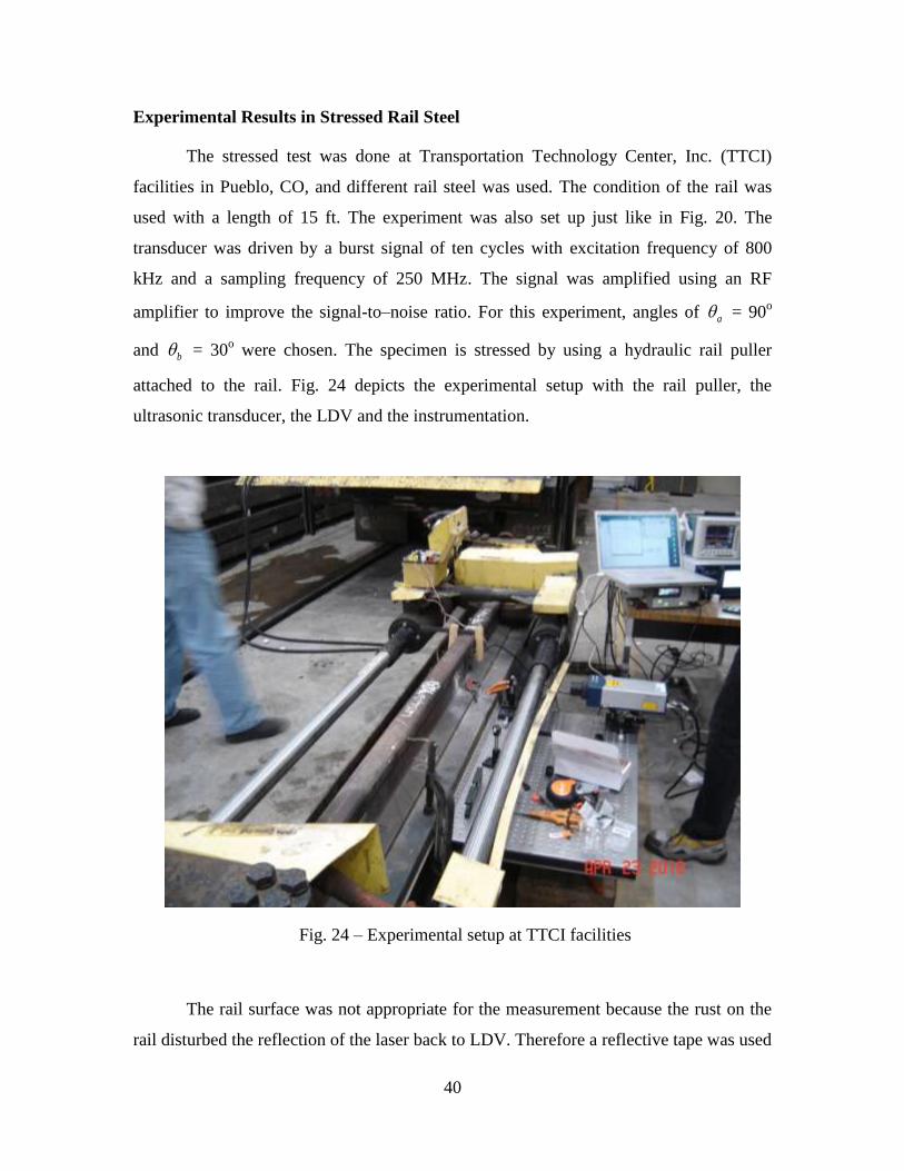
Experimental Results in Stressed Rail Steel
The stressed test was done at Transportation Technology Center, Inc. (TTCI)
facilities in Pueblo, CO, and different rail steel was used. The condition of the rail was
used with a length of 15 ft. The experiment was also set up just like in Fig. 20. The
transducer was driven by a burst signal of ten cycles with excitation frequency of 800
kHz and a sampling frequency of 250 MHz. The signal was amplified using an RF
amplifier to improve the signal-to–noise ratio. For this experiment, angles of a = 90o
and b = 30
o were chosen. The specimen is stressed by using a hydraulic rail puller
attached to the rail. Fig. 24 depicts the experimental setup with the rail puller, the
ultrasonic transducer, the LDV and the instrumentation.
The rail surface was not appropriate for the measurement because the rust on the
rail disturbed the reflection of the laser back to LDV. Therefore a reflective tape was used
Fig. 24 – Experimental setup at TTCI facilities
41
on the rail surface. Once the out-of-plane measurement and 30o angle measurement were
acquired, the data was processed using MATLAB, and the ratio between in-plane and
out-of-plane component was calculated to get the Polarization of Rayleigh wave.
The experiment was done on the rail under different loads. During the
compression test, some of the rail puller clamps slipped. The rail experienced bending
and torsional moment during compression, causing the rail to “jump” when the
compression load exceeded a specific value. This “jump” caused the movement of the
wedge transducer. Furthermore, due to the slipping of the rail puller the stress in the rail
was not constant over time. The current setup requires the measurement at two different
angles. With the restriction of a single LDV, these measurements cannot be done
simultaneously. Hence, the data of the compression test are excluded in this report.
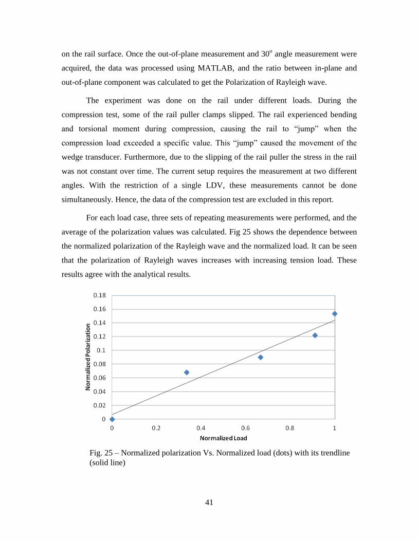
For each load case, three sets of repeating measurements were performed, and the
average of the polarization values was calculated. Fig 25 shows the dependence between
the normalized polarization of the Rayleigh wave and the normalized load. It can be seen
that the polarization of Rayleigh waves increases with increasing tension load. These
results agree with the analytical results.
Fig. 25 – Normalized polarization Vs. Normalized load (dots) with its trendline
(solid line)
42
The experiment at TTCI shows that the Rayleigh wave polarization depends on
the longitudinal force of the rail. However, further research is recommended in order to
solve the inverse problem, where the longitudinal force in the rail can be determined from
the polarization of the Rayleigh wave. Follow on investigations are suggested to study the
effect of the rail surface quality (polishing, sanding, grinding, blasting etc.) on the
measured results. It would be useful to further investigate the effect of focusing of the
laser vibrometer.
The design, manufacturing and thorough testing of a prototype would be the next
step. Thereby, potential funding by Transportation Technology Center Inc. (TTCI) and
Southwest University Transportation Center (SWUTC) is considered.
43
CHAPTER 6
Conclusions
This research investigated a method of determining the stress in rails by using the
polarization of Rayleigh waves. The relationship between the polarization of Rayleigh
waves and the state of stress is developed from the analytical model. The numerical
simulation showed that the change of polarization of Rayleigh wave on residual stress is
one order of magnitude higher than the change of Rayleigh wave speed. Additionally,
sensitivity analysis showed that the polarization of a Rayleigh wave is more robust
against uncertainties in material properties. These results concluded that Rayleigh wave
polarization is more sensitive and more robust than the Rayleigh wave speed. These are
the two main reasons why Rayleigh wave polarization was used instead of Rayleigh wave
speed.
This method is a non-destructive and non-labor intensive measurement
technique. The measurement of polarization is a point wise measurement, meaning that
the applied stress on rail can be determined just by measuring the polarization from a
single point. This method is also a reference-free measurement. No information about the
propagation distance is needed to perform the measurement. The combination of these
benefits is the advantage of this method that other methods do not have.
The results of the numerical simulation were verified with the preliminary
experimental results. Further measurements were done in a stressed rail and the change in
polarization of the Rayleigh wave was determined using a wedge transducer for
generation and a laser Doppler vibrometer for the detection of ultrasonic waves. After a
thorough evaluation, the concept was tested at Transportation Technology Center, Inc.
(TTCI) facilities in Pueblo, CO, to transfer the developed technology to TTCI researches
and Association of American Railroads (AAR) members. The results showed that the
polarization of Rayleigh wave changes with longitudinal stress. Knowing the longitudinal
stress will prevent future buckling of the rail and reduce the number of derailments and
increase railroad safety.

44
The design, manufacturing and thorough testing of a prototype will be the next
step. Thereby, potential funding by Transportation Technology Center Inc. (TTCI) and
Southwest University Transportation Center (SWUTC) is considered.
45
REFERENCES
D. M. Egle and E. D. Bray (1976): Measurement of acousto-elastic and third-order elastic
constants for rail steel, Journal of the Acoustical Society of America, Vol. 60, pp. 741-
744.
D. M. Egle and E. D. Bray (1979): Application of the Acousto-Elastic Effect to Rail
Stress Measurements. Material Evaluation, Vol. 37, pp. 41-55.
D. Read, B. Shust (2007). Railway Track & Structures. New York: Jun 2007. Vol.
103(6), pp. 19.
M. Junge. Measurement of Applied Stresses Using the Polarization of Rayleigh Surface
Waves, M.S. Thesis. University of Stuttgart: November 2003.
M. Junge, and J. Qu, and L. J. Jacobs (2006): Relationship Between Rayleigh Wave
Polarization and State of Stress, Ultrasonics Journal, Vol. 44(3), pp. 233-237.
D. I. Crecraft (1962): Ultrasonic wave velocities in stresses nickel steel, Nature, Vol.
195(4847), pp.1193.
D. I. Crecraft (1967): The Measurement of Applied and Residual Stresses in Metals for
Measurement of Contained Stress in Railroad Rail, Journal and Sound Vibration, Vol.
5(1), pp. 173-192.
A. Kish and G. Samavedam (2005): Improved Destressing of Continuous Welded Rail
for Better Management of Rail Neutral Temperature, Journal of the Transportation
Research Board, Vol.1916, pp. 56-65.
A. Kish and D. Read (2006): Proceedings of the Workshop on CWR Track Stability,
Pueblo CO, March 15, 2006
V. Damljanovic and R.L. Weaver (2005): Laser vibrometer technique for measurement of
contained stress in railroad rail, Journal of Sound and Vibration, Vol.282, pp. 341-366.
46
M. Duquennoy, and M.Ouaftough, and M.Ourak (1999): Ultrasonic Evaluation of
Stresses in Orthotropic Materials Using Rayleigh Waves, NDT&E International, Vol.
32(4), pp. 189-199.
M. Duquennoy, and M.Ouaftough, and M.L.Qian, F.Jenot and M.Ourak (2001):
Ultrasonic Characterization of Residual Stresses in Steel Rods Using a Laser Line Source
and Piezoelectric Transducers, NDT&E International, Vol. 34(5), pp. 355-362.
S. Hurlebaus (1996): Laser Generation and Detection Techniques for Developing
Transfer Functions to Characterize the Effect of Geometry on Elastic Wave Propagation,
M.S. thesis, School of Civil and Environmental Engineering, Georgia Institute of
Technology, Atlanta, GA.
S. Hurlebaus (2002a): A Contribution to Structural Health Monitoring Using Elastic
Waves, PhD thesis, Institute A of Mechanics, University of Stuttgart, Stuttgart, Germany
S. Hurlebaus (2002b): Laser Ultrasonics for Structural Health Monitoring, Contribution
to the 7th Laser-Vibrometer Seminar, Polytec, Waldbronn, Vol. 1 , pp. 1-27.
S. Hurlebaus and L.J. Jacobs (2006): Dual Probe Laser Interferometer for Structural
Health Monitoring, Journal of the Acoustical Society of America, Vol. 119(4), pp. 1923-
1925.
M. Hirao, M. and H. Fukuoka, H. and K. Hori (1981): Acoustoelastic Effect of Rayleigh
Surface Wave in Isotropic Material, Journal of Applied Mechanics, Vol. 48, pp. 119-124.
Y. H. Pao, and W. Sachse, and H.Fukuoka, (1984): Acoustoelasticity and Ultrasonic
Measurements of Residual Stresses, Physical Acoustics, Vol. 17, pp. 61-143.
F. D. Murnaghan (1951). Finite Deformation of an Elastic Solid, Wiley, New York.
J. L. Rose (1999). Ultrasonic Waves in Solid Media. Cambridge University Press.
D. S. Hughes and J. L. Kelly. Second-Order Elastic Deformation of Solids. Physical
Review, Vol. 92(5), pp. 1145-1149. December 1953.
R.T. Smith, R. Stern, and R.W.B. Stephens (1966). Third-Order Elastic Moduli of
Polycrystalline Metals from Ultrasonic Velocity Measurements. Journal of the Acoustical
Society of America, Vol. 40(5), pp. 1002-1008.
47
R.A. Toupin and B. Bernstein (1961). Sound Waves in Deformed Perfectly Elastic
Materials. Acoustoelastic Effect. Journal of the acoustical Society of America, Vol.
33(2), pp. 216-225.
Y. H. Pao and U. Gamer (1985). Acoustoelastic Waves in Orthotropic Media. Journal of
the Acoustical Society of America, Vol. 77(3), pp. 806.
B. Masserey and P. Fromme (2008). On The Reflection of Coupled Rayleigh-like Waves
At Surface Defects in Plates, Journal of the Acoustical Society of America, Vol. 123, pp.
88 - 98.
I.A. Viktorov (1966). Rayleigh and Lamb Waves. Plenum Press, New York, NY.
K.F. Graff (1991). Wave Motion in Elastic Solids. Dover Publications Inc., New York.
H. G. Kil, J. Jarzynski, and Y. H. Berthelot (1998). Wave Decomposition of The
Vibrations of A Cylindrical Shell With An Automated Scanning Laser Vibrometer.
Journal of the acoustical Society of America, Vol. 104(6), pp. 3161-3168.
48
INVESTIGATOR PROFILE
Dr. Hurlebaus, Assistant Professor at Texas A&M University, is the Principal
Investigator. His contact information is:
Dr.-Ing. Stefan Hurlebaus
Zachry Department of Civil Engineering
Texas Transportation Institute (TTI)
Texas A&M University
3136 TAMU
College Station, TX 77843-3136
USA
phone: (979) 845-9570
fax: (979) 845-6554
email: [email protected]


![[Rock'n Rails] Deploying Rails Applications with Capistrano](https://img.pdfslide.us/doc/110x75/54bae7b84a7959086c8b4589/rockn-rails-deploying-rails-applications-with-capistrano.jpg)