Determination of the initial beam parameters in Monte Carlo linac simulationKhaled Aljarrah, Greg C. Sharp, Toni Neicu, and Steve B. Jiang

Citation: Medical Physics 33, 850 (2006); doi: 10.1118/1.2168433 View online: http://dx.doi.org/10.1118/1.2168433 View Table of Contents: http://scitation.aip.org/content/aapm/journal/medphys/33/4?ver=pdfcov Published by the American Association of Physicists in Medicine Articles you may be interested in Monte Carlo simulation of TrueBeam flattening-filter-free beams using Varian phase-space files: Comparisonwith experimental data Med. Phys. 41, 051707 (2014); 10.1118/1.4871041 A Monte Carlo approach to validation of FFF VMAT treatment plans for the TrueBeam linac Med. Phys. 40, 021707 (2013); 10.1118/1.4773883 Monte Carlo linear accelerator simulation of megavoltage photon beams: Independent determination of initialbeam parameters Med. Phys. 39, 40 (2012); 10.1118/1.3668315 Inference of the optimal pretarget electron beam parameters in a Monte Carlo virtual linac model throughsimulated annealing Med. Phys. 36, 2309 (2009); 10.1118/1.3130102 Monte Carlo simulation estimates of neutron doses to critical organs of a patient undergoing 18 MV x-ray LINAC-based radiotherapy Med. Phys. 32, 3579 (2005); 10.1118/1.2122547

Determination of the initial beam parameters in Monte Carlo linacsimulation

Khaled AljarrahDepartment of Physics, University of Massachusetts Lowell, Lowell, Massachusetts

Greg C. Sharp, Toni Neicu, and Steve B. Jianga�

Department of Radiation Oncology, Massachusetts General Hospital and Harvard Medical School, Boston,Massachusetts

�Received 1 November 2005; revised 13 December 2005; accepted for publication 30 December 2005;published 13 March 2006�

For Monte Carlo linac simulations and patient dose calculations, it is important to accuratelydetermine the phase space parameters of the initial electron beam incident on the target. Theseparameters, such as mean energy and radial intensity distribution, have traditionally been deter-mined by matching the calculated dose distributions with the measured dose distributions through atrial and error process. This process is very time consuming and requires a lot of Monte Carlosimulation experience and computational resources. In this paper, we propose an easy, efficient, andaccurate method for the determination of the initial beam parameters. We hypothesize that �1� forone type of linacs, the geometry and material of major components of the treatment head are thesame; the only difference is the phase space parameters of the initial electron beam incident on thetarget, and �2� most linacs belong to a limited number of linac types. For each type of linacs, MonteCarlo treatment planning system �MC-TPS� vendors simulate the treatment head and calculate thethree-dimensional �3D� dose distribution in water phantom for a grid of initial beam energies andradii. The simulation results �phase space files and dose distribution files� are then stored in a datalibrary. When a MC-TPS user tries to model their linac which belongs to the same type, a standardset of measured dose data is submitted and compared with the calculated dose distributions todetermine the optimal combination of initial beam energy and radius. We have applied this methodto the 6 MV beam of a Varian 21EX linac. The linac was simulated using EGSNRC/BEAM code andthe dose in water phantom was calculated using EGSNRC/DOSXYZ. We have also studied issuesrelated to the proposed method. Several common cost functions were tested for comparing mea-sured and calculated dose distributions, including �2, mean absolute error, dose difference at thepenumbra edge point, slope of the dose difference of the lateral profile, and the newly proposed ��

factor �defined as the fraction of the voxels with absolute dose difference less than �%�. It wasfound that the use of the slope of the lateral profile difference or the difference of the penumbraedge points may lead to inaccurate determination of the initial beam parameters. We also found thatin general the cost function value is very sensitive to the simulation statistical uncertainty, and thereis a tradeoff between uncertainty and specificity. Due to the existence of statistical uncertainty insimulated dose distributions, it is practically impossible to determine the best energy/radius com-bination; we have to accept a group of energy/radius combinations. We have also investigated theminimum required data set for accurate determination of the initial beam parameters. We found thatthe percent depth dose curves along or only a lateral profile at certain depth for a large field size isnot sufficient and the minimum data set should include several lateral profiles at various depths aswell as the central axis percent depth dose curve for a large field size. © 2006 American Associa-tion of Physicists in Medicine. �DOI: 10.1118/1.2168433�

Key words: Monte Carlo, treatment planning, commissioning, linac simulation

I. INTRODUCTION

Previous studies have demonstrated that the Monte Carlosimulation is an accurate method for dose calculation in ra-diotherapy �e.g., Refs. 1–5�. Accurate dose calculation re-quires precise characterization of the accelerator geometryand parametrization of the initial electron beam incident onthe target. Any error in determining the beam parameters will

cause a systematic error in patient dose calculation. The de-

850 Med. Phys. 33 „4…, April 2006 0094-2405/2006/33„4

termination of the initial beam parameters is a challengingpart in linac modeling with the Monte Carlo method, andalso is an important issue for implementing Monte Carlodose calculation in treatment planning.

Over the years, much effort has been devoted to a varietyof issues concerning the Monte Carlo modeling of linearaccelerator �e.g., Refs. 6–16�, but very few studies have fo-cused on determination of the initial electron beam charac-

teristics. One comprehensive study was performed by

850…/850/9/$23.00 © 2006 Am. Assoc. Phys. Med.

851 Aljarrah et al.: Monte Carlo Linac Simulation 851

Sheikh-Bagheri and Rogers,17,18 which investigated the ef-fect of the initial electron beam parameters on photon beamdose distributions. Their conclusions show that the most im-portant parameters of the incident electron beam are the ra-dial intensity distribution and the mean energy. Anotherstudy done by Keall et al.19 investigated three beam param-eters: mean electron energy, electron radial spread, and targetdensity. The study was performed by varying one parameterwhile fixing the other two. They found that the target densitydoes not play an important role in the determination of initialelectron beam fluence. In the study of Tzedakis et al.,20 themean energy was fixed first and the beam radius was deter-mined by minimizing a quadratic function which fits the ab-solute difference of the dose at the penumbra edge point.Then the determined value of the beam radius was fixed andthe beam energy was determined in the same way.

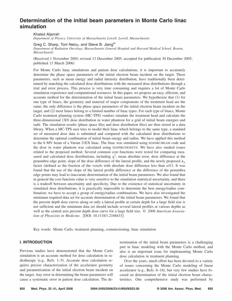
In most of other previous studies the beam parameterswere determined by matching the calculated dose distribu-tions with the measured dose distributions through a trial anderror process.7,21–26 Figure 1 shows a flowchart illustratingmain steps of this method. It starts with an initial guess of thebeam parameters. Then the treatment head of the linac issimulated and the three-dimensional �3D� dose distributionin water phantom is calculated, both using the Monte Carlomethod. The calculated dose distribution is compared withthe measured dose distribution by either visually inspectingthe dose curves plotted together or using a certain cost func-tion �such as the chi-square function�. If the simulationagrees with the measurement within the preset tolerance, theinitial parameters are accepted and the process ends; other-wise, the parameters are tuned based on the dose differenceand a new iteration starts. This method is very time consum-ing because the time needed to create a single 3D dose file isabout 30 to 40 h on a 2 GHz Pentium 4 processor. Thereforecommissioning of one beam may take weeks, especially forthose Monte Carlo treatment planning system �MC-TPS� us-ers who have little Monte Carlo simulation experience. An-other weakness of this approach is that the iteration may endwith a suboptimal solution since the solution space may have

FIG. 1. The flowchart represents the trial and error process usually used todetermine the initial beam parameters for Monte Carlo linac simulation.

local minima.

Medical Physics, Vol. 33, No. 4, April 2006

In this paper, we will present a new commissioning strat-egy as a solution to the above mentioned problems. Someissues related to the determination of initial beam param-eters, such as the cost functions used for dose comparisonand the minimum data set required for the comparison, willalso be discussed.

II. NEW STRATEGY FOR DETERMINING THEINITIAL BEAM PARAMETERS

By analyzing the current procedure for the determinationof the initial beam parameters, we realized that the simula-tion of linac treatment head should be performed �1� bysomeone with Monte Carlo expertise and computational re-sources �such as MC-TPS vendors�, instead of inexperiencedgeneral MC-TPS users, and �2� only once for the same typeof linacs. Consequently, we have developed a new strategyfor determining the initial beam parameters in an accurateand fast fashion �a few seconds for MC-TPS users�.

The new strategy for determining the initial beam param-eters is based on two observations:

1. Same type of linacs �such as Varian 21EX 6 MV photonbeam� are the same or similar enough in the geometryand material of key components and only differ by thephase space parameters of the initial electron beam inci-dent on the target.

2. Most existing linacs belong to a limited number of linactypes.

Hence, the simulation of a linac treatment head with a largerange of initial beam parameters should cover all the linacsof the same type. The two important initial beam parameters,energy and radius, as pointed out by Sheikh-Bagheri et al.,27

are considered in this work. We assume the initial electronbeam is a monodirectional, monoenergetic beam with aGaussian intensity distribution.

The new strategy consists of the following steps:

1. An MC-TPS vendor simulates the treatment heads forvarious types of linacs for a large range of energy andradius of initial electron beam incident on the target. Theenergy values should be around the nominal energy withsufficient variation, and the radius values should cover arange of possible radius values. For each energy/radiuscombination, a beam phase space file with a sufficientnumber of particles is saved at the level right above thejaws.

2. The MC-TPS vendor calculates dose distributions in awater phantom using the saved phase space file as inputfor each energy/radius combination. The calculated dosedistributions are stored.

3. When a MC-TPS user tries to commission a linac forMonte Carlo treatment planning, the user acquires astandard set of measured dose distributions in waterphantom as specified by the MC-TPS vendor.

4. The user uses a computer code provided by the vendor

to compare the measured dose data with the calculated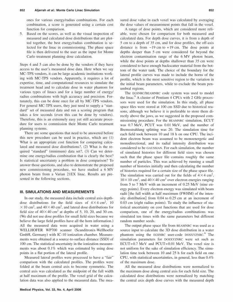

852 Aljarrah et al.: Monte Carlo Linac Simulation 852

ones for various energy/radius combinations. For eachcombination, a score is generated using a certain costfunction for comparison.

5. Based on the scores, as well as the visual inspection ofmeasured and calculated dose distributions that are plot-ted together, the best energy/radius combination is se-lected for the linac in commissioning. The phase spacefile is then delivered to the user as the input for MonteCarlo treatment planning dose calculation.

Steps 4 and 5 can also be done by the vendors if they haveaccess to the user’s measured dose data. Here when we sayMC-TPS vendors, it can be large academic institutions work-ing with MC-TPS vendors. Apparently, it requires a lot ofexpertise, time, and computational resources to simulate thetreatment head and to calculate dose in water phantom forvarious types of linacs and for a large number of energy/radius combinations with high accuracy and precision. For-tunately, this can be done once for all by MC-TPS vendors.For general MC-TPS users, they just need to supply a “stan-dard” set of measured data and run a scoring program thattakes a few seconds �even this can be done by vendors�.Therefore, this is an extremely easy yet still accurate proce-dure for users to commission their Monte Carlo treatmentplanning systems.

There are some questions that need to be answered beforethis new procedure can be used in practice, which are �1�What is an appropriate cost function for comparing calcu-lated and measured dose distributions?, �2� What is the re-quired “standard” �minimum� data set?, �3� Can we deter-mine one energy/radius combination that is clearly the best?Is statistical uncertainty a problem in dose comparison? Toanswer those questions, and also to demonstrate the proposednew commissioning procedure, we have studied a 6 MVphoton beam from a Varian 21EX linac. Results are pre-sented in the following sections.

III. SIMULATIONS AND MEASUREMENTS

In our study, the measured data include central axis depth-dose distributions for the field sizes of 4�4 cm2, 10�10 cm2, and 40�40 cm2, and lateral dose distributions forfield size of 40�40 cm2 at depths of 5, 10, 20, and 30 cm.�We did not use dose profiles for small field sizes because webelieve the large field profiles have all the horn information.�All the measured data were acquired in water using aWELLHOFER WP700 scanner �Scanditronix-WellhoeferGmbH, Germany� with IC-10 ionization chamber. Measure-ments were obtained at a source-to-surface distance �SSD� of100 cm. The statistical uncertainty in the ionization measure-ments was about 0.1% which was estimated by using dosepoints in a flat portion of the lateral profile.

Measured lateral profiles were processed to have a “fair”comparison with the calculated profiles. The profiles werefolded at the beam central axis to become symmetric. Thecentral axis was calculated as the midpoint of the full widthat half maximum of the profile. The voxel grid of the calcu-

lation data was also applied to the measured data. The mea-

Medical Physics, Vol. 33, No. 4, April 2006

sured dose value in each voxel was calculated by averagingthe dose values of measurement points that fall in the voxel.

A range of dose points, which are considered more reli-able, were chosen for comparison for both measured andcalculated data. For depth dose curves, it is from a depth of5 cm to a depth of 35 cm, and for dose profiles, the off-axisdistance is from −19 cm to +19 cm. The dose points atdepths deeper than 5 cm were considered far beyond theelectron contamination range of the 6 MV photon beam,while the dose points at depths shallower than 35 cm wereconsidered to have enough backscatter material from the bot-tom of the water tank. The choice of the boundary for thelateral profile curves was made to include the horns of theprofile, which is the most sensitive region to the variation inthe initial beam parameters, while to exclude the beam pen-umbral regions.

The EGSNRC/BEAMNRC code system was used to modelthe linac.6 A cluster of Pentium 4 CPUs with 2 GHz proces-sors were used for the simulation. In this study, all phasespace files were stored at 100 cm SSD due to historical rea-sons, although we believe it is preferable to store them di-rectly above the jaws, as we suggested in the proposed com-missioning procedure. For the BEAMNRC simulation, ECUTwas 0.7 MeV, PCUT was 0.01 MeV, and the number ofBremsstrahlung splitting was 20. The simulation time foreach field took between 10 and 18 h on one CPU. The inci-dent electron beam was assumed to be monoenergetic andmonodirectional, and its radial intensity distribution wasconsidered to be GAUSSIAN. For each simulation, the numberof simulated histories for different field sizes was chosensuch that the phase space file contains roughly the samenumber of particles. This was achieved by running a smallnumber of histories initially and then calculating the numberof histories required for a certain size of the phase space file.The simulation was carried out for the fields of 4�4 cm2,10�10 cm2, and 40�40 cm2 over electron energies rangingfrom 5 to 7 MeV with an increment of 0.25 MeV �nine en-ergy points�. Every electron energy was simulated with beamradii �the full width at half maximum �FWHM� of the inten-sity distribution� from 0.04 to 0.25 cm at an increment of0.03 cm �eight radius points�. To study the influence of sta-tistical uncertainty on cost functions that are used for dosecomparison, one of the energy/radius combinations wassimulated ten times with the same parameters but differentrandom number seeds.

The output phase space file from BEAMNRC was used as asource input to calculate the 3D dose distribution in a waterphantom using the EGSNRC user-code DOSXYZNRC.6 Thesimulation parameters for DOSXYZNRC were set such asECUT=0.7 MeV and PCUT=0.01 MeV. The voxel size isnot uniform for the sake of simulation efficiency. The simu-lation time took between 10 and 25 h for each field on oneCPU, with statistical uncertainties, in general, less than 0.4%of the maximum dose.

All the measured dose distributions were normalized tothe maximum dose along central axis for each field size. Thecalculated dose distributions were normalized by matching

the central axis depth dose curves with the measured depth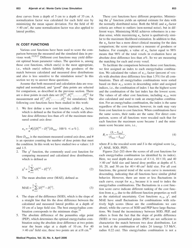

853 Aljarrah et al.: Monte Carlo Linac Simulation 853

dose curves from a depth of 5 cm to a depth of 35 cm. Anormalization factor was calculated for each field size byminimizing the mean square deviation. For the field of 40�40 cm2, the same normalization factor was also applied tolateral profiles.

IV. COST FUNCTIONS

Various cost functions have been used to score the com-parison between the measured and the simulated data in pre-vious work.19,20,27 Different cost functions may yield differ-ent optimal beam parameter values. The question is, amongthose cost functions, which one�s� is the most appropriate,i.e., which one�s� reflects faithfully the goodness of thematch between calculated and measured dose distributionsand also is less sensitive to the simulation noise? In thissection we try to answer those questions.

Assume that both measured and calculation data are resa-mpled and normalized, and “good” data points are selectedfor comparison, as described in the previous section. Thereare n dose points in each data set �D1

�m� ,D2�m� , . . . . . . ,Dn

�m� formeasurement and D1

�s� ,D2�s� , . . . . . . ,Dn

�s� for simulation�. Thefollowing cost functions have been studied in this work:

1. We first define a new cost function, called �� factor,which is defined as the fraction of the voxels with abso-lute dose difference less than �% of the maximum mea-sured central axis dose:

�� =1

n#�i��Di

�m� − Di�s��/Dmax · 100 % � � % � . �1�

Here Dmax is the maximum measured central axis dose, and #is an operator counting the number of dose points that meetthe condition. In this work we have studied two � values: 1.0and 1.5.2. The �2 function, the commonly used cost function for

comparing measured and calculated dose distributions,which is defined as

�2 =1

n�i=1

n

�Di�m� − Di

�s��2. �2�

3. The mean absolute error �MAE�, defined as

MAE =1

n�i=1

n

�Di�m� − Di

�s�� . �3�

4. The slope of the difference �SOD�, which is the slope ofa straight line that fits the dose difference between thecalculated and measured lateral profiles at a depth of10 cm of a large field size. The best energy/radius com-bination corresponds to the minimum slope.19

5. The absolute difference of the penumbra edge point�PEP�, which determines the optimal energy/radius com-bination using the absolute dose difference at two pointsnear the beam edge at a depth of 10 cm. For 40

2 20

�40 cm field size, these two points are at ±18 cm.

Medical Physics, Vol. 33, No. 4, April 2006

These cost functions have different properties. Minimiz-ing the �2 function yields an optimal estimate for data withthe normally distributed noise. Both the MAE and ��-factorcriteria are robust to outliers �non-normal noise�, but in dif-ferent ways. Minimizing MAE achieves robustness in a me-dian sense, while maximizing �� factor is qualitatively simi-lar to the maximum likelihood estimation. In addition to that,the �� factor has a more direct clinical meaning for the datacomparison; the score represents a measure of goodness orbadness. For example, a value of �� factor equal to 98%means that 98% of the total voxels in evaluation have anabsolute dose difference less than �%. So we are measuringthe matching for each and every voxel.

To facilitate the comparison between those cost functions,we first assigned an index to each energy/radius combina-tion. We calculated the values of �1.5 factor �percent of vox-els with absolute dose difference less than 1.5%� for all com-binations. Then all energy/radius combinations were sortedbased on their �1.5 scores in descending order and assignedindices, i.e., the combination of index 1 has the highest scoreand the combination of the last index has the lowest score.The values of all other cost functions, including �1.0, werealso calculated and used to rank an energy/radius combina-tion. For an energy/radius combination, the index is the sameregardless of the cost function; however, its rank may varyfrom cost function to cost function. When combinations havethe same scores, their ranks are the same. For direct com-parison, scores of all functions were rescaled such that foreach function the maximum score became 1 and the mini-mum score became zero, i.e.,

Ri =�Si − Smin�

�Smax − Smin�, �4�

where R is the rescaled score and S is the original score ���,�2, MAE, SOD, PEP�.

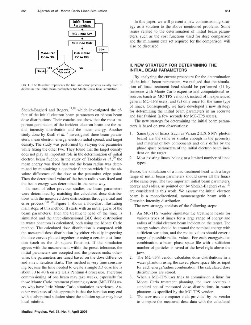
Figures 2�a�–2�f� show the scores of all cost functions foreach energy/radius combination �as identified by its index�.Here, we used depth dose curves of 4�4, 10�10, and 40�40 cm2 field size and lateral dose profiles at depths of 5,10, 20, and 30 cm for 40�40 cm2 field size. For all costfunctions, the general trend of the score curve is monotonicdescending, indicating that all functions have similar globalbehavior. However, there are more or less fluctuations ineach curve, except for �1.5 because it is used to index theenergy/radius combinations. The fluctuations in a cost func-tion score curve indicate different ranking of the cost func-tion from �1.5, due to the different function properties as wellas the statistical uncertainty. Cost functions �1.0, �2, andMAE have small fluctuations for combinations with rela-tively high scores �those are the combinations we careabout�, while the curves of SOD and PEP have large fluctua-tions. We found the inconsistency between SOD, PEP, andothers is from the fact that the slope of profile difference�SOD� or two penumbral points �PEP� are not sufficient tocharacterize the match between two dose distributions. Letus look at the combination of index 24 �energy 5.5 MeV,

radius 0.22 cm�. This energy/radius combination is not a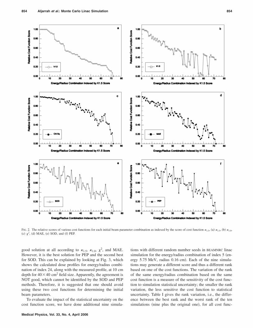

854 Aljarrah et al.: Monte Carlo Linac Simulation 854

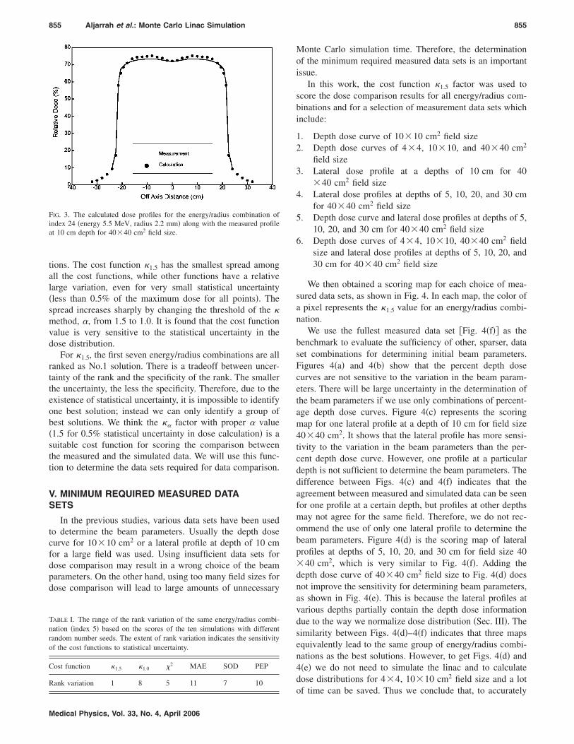
good solution at all according to �1.5, �1.0, �2, and MAE.However, it is the best solution for PEP and the second bestfor SOD. This can be explained by looking at Fig. 3, whichshows the calculated dose profiles for energy/radius combi-nation of index 24, along with the measured profile, at 10 cmdepth for 40�40 cm2 field size. Apparently, the agreement isNOT good, which cannot be identified by the SOD and PEPmethods. Therefore, it is suggested that one should avoidusing these two cost functions for determining the initialbeam parameters.

To evaluate the impact of the statistical uncertainty on the

FIG. 2. The relative scores of various cost functions for each initial beam par�c� �2, �d� MAE, �e� SOD, and �f� PEP.

cost function score, we have done additional nine simula-

Medical Physics, Vol. 33, No. 4, April 2006

tions with different random number seeds in BEAMNRC linacsimulation for the energy/radius combination of index 5 �en-ergy 5.75 MeV, radius 0.16 cm�. Each of the nine simula-tions may generate a different score and thus a different rankbased on one of the cost functions. The variation of the rankof the same energy/radius combination based on the samecost function is a measure of the sensitivity of the cost func-tion to simulation statistical uncertainty; the smaller the rankvariation, the less sensitive the cost function to statisticaluncertainty. Table I gives the rank variation, i.e., the differ-ence between the best rank and the worst rank of the ten

r combination as indexed by the score of cost function �1.5, �a� �1.5, �b� �1.0,

amete

simulations �nine plus the original one�, for all cost func-

855 Aljarrah et al.: Monte Carlo Linac Simulation 855

tions. The cost function �1.5 has the smallest spread amongall the cost functions, while other functions have a relativelarge variation, even for very small statistical uncertainty�less than 0.5% of the maximum dose for all points�. Thespread increases sharply by changing the threshold of the �method, �, from 1.5 to 1.0. It is found that the cost functionvalue is very sensitive to the statistical uncertainty in thedose distribution.

For �1.5, the first seven energy/radius combinations are allranked as No.1 solution. There is a tradeoff between uncer-tainty of the rank and the specificity of the rank. The smallerthe uncertainty, the less the specificity. Therefore, due to theexistence of statistical uncertainty, it is impossible to identifyone best solution; instead we can only identify a group ofbest solutions. We think the �� factor with proper � value�1.5 for 0.5% statistical uncertainty in dose calculation� is asuitable cost function for scoring the comparison betweenthe measured and the simulated data. We will use this func-tion to determine the data sets required for data comparison.

V. MINIMUM REQUIRED MEASURED DATASETS

In the previous studies, various data sets have been usedto determine the beam parameters. Usually the depth dosecurve for 10�10 cm2 or a lateral profile at depth of 10 cmfor a large field was used. Using insufficient data sets fordose comparison may result in a wrong choice of the beamparameters. On the other hand, using too many field sizes fordose comparison will lead to large amounts of unnecessary

FIG. 3. The calculated dose profiles for the energy/radius combination ofindex 24 �energy 5.5 MeV, radius 2.2 mm� along with the measured profileat 10 cm depth for 40�40 cm2 field size.

TABLE I. The range of the rank variation of the same energy/radius combi-nation �index 5� based on the scores of the ten simulations with differentrandom number seeds. The extent of rank variation indicates the sensitivityof the cost functions to statistical uncertainty.

Cost function �1.5 �1.0 �2 MAE SOD PEP

Rank variation 1 8 5 11 7 10

Medical Physics, Vol. 33, No. 4, April 2006

Monte Carlo simulation time. Therefore, the determinationof the minimum required measured data sets is an importantissue.

In this work, the cost function �1.5 factor was used toscore the dose comparison results for all energy/radius com-binations and for a selection of measurement data sets whichinclude:

1. Depth dose curve of 10�10 cm2 field size2. Depth dose curves of 4�4, 10�10, and 40�40 cm2

field size3. Lateral dose profile at a depths of 10 cm for 40

�40 cm2 field size4. Lateral dose profiles at depths of 5, 10, 20, and 30 cm

for 40�40 cm2 field size5. Depth dose curve and lateral dose profiles at depths of 5,

10, 20, and 30 cm for 40�40 cm2 field size6. Depth dose curves of 4�4, 10�10, 40�40 cm2 field

size and lateral dose profiles at depths of 5, 10, 20, and30 cm for 40�40 cm2 field size

We then obtained a scoring map for each choice of mea-sured data sets, as shown in Fig. 4. In each map, the color ofa pixel represents the �1.5 value for an energy/radius combi-nation.

We use the fullest measured data set �Fig. 4�f�� as thebenchmark to evaluate the sufficiency of other, sparser, dataset combinations for determining initial beam parameters.Figures 4�a� and 4�b� show that the percent depth dosecurves are not sensitive to the variation in the beam param-eters. There will be large uncertainty in the determination ofthe beam parameters if we use only combinations of percent-age depth dose curves. Figure 4�c� represents the scoringmap for one lateral profile at a depth of 10 cm for field size40�40 cm2. It shows that the lateral profile has more sensi-tivity to the variation in the beam parameters than the per-cent depth dose curve. However, one profile at a particulardepth is not sufficient to determine the beam parameters. Thedifference between Figs. 4�c� and 4�f� indicates that theagreement between measured and simulated data can be seenfor one profile at a certain depth, but profiles at other depthsmay not agree for the same field. Therefore, we do not rec-ommend the use of only one lateral profile to determine thebeam parameters. Figure 4�d� is the scoring map of lateralprofiles at depths of 5, 10, 20, and 30 cm for field size 40�40 cm2, which is very similar to Fig. 4�f�. Adding thedepth dose curve of 40�40 cm2 field size to Fig. 4�d� doesnot improve the sensitivity for determining beam parameters,as shown in Fig. 4�e�. This is because the lateral profiles atvarious depths partially contain the depth dose informationdue to the way we normalize dose distribution �Sec. III�. Thesimilarity between Figs. 4�d�–4�f� indicates that three mapsequivalently lead to the same group of energy/radius combi-nations as the best solutions. However, to get Figs. 4�d� and4�e� we do not need to simulate the linac and to calculatedose distributions for 4�4, 10�10 cm2 field size and a lot

of time can be saved. Thus we conclude that, to accurately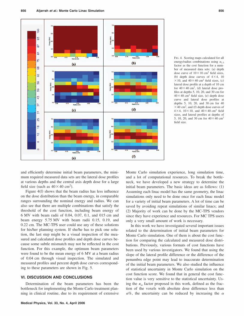

856 Aljarrah et al.: Monte Carlo Linac Simulation 856

and efficiently determine initial beam parameters, the mini-mum required measured data sets are the lateral dose profilesat various depths and the central axis depth dose for a largefield size �such as 40�40 cm2�.

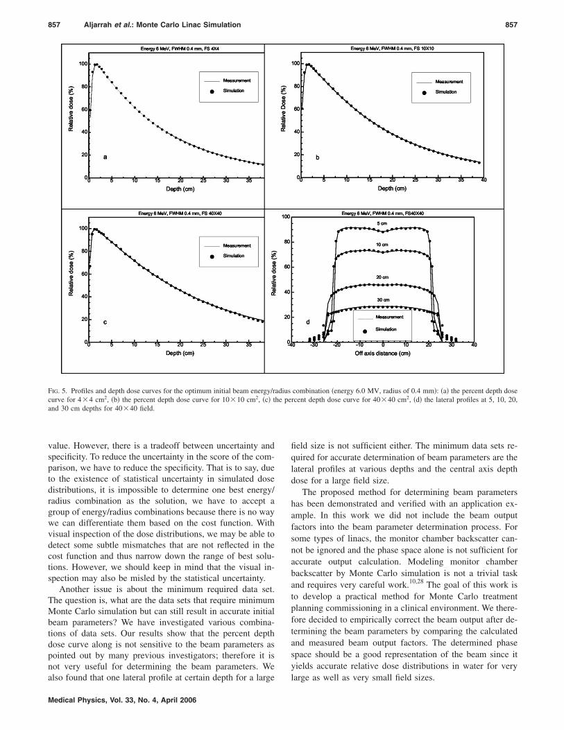
Figure 4�f� shows that the beam radius has less influenceon the dose distribution than the beam energy, in comparableranges surrounding the nominal energy and radius. We canalso see that there are multiple combinations that satisfy thethreshold of the cost function, including beam energy of6 MV with beam radii of 0.04, 0.07, 0.1, and 015 cm andbeam energy 5.75 MV with beam radii 0.15, 0.19, and0.22 cm. The MC-TPS user could use any of these solutionsfor his/her planning system. If she/he has to pick one solu-tion, the last step might be a visual inspection of the mea-sured and calculated dose profiles and depth dose curves be-cause some subtle mismatch may not be reflected in the costfunction. For this example, the optimum beam parameterswere found to be the mean energy of 6 MV at a beam radiusof 0.04 cm through visual inspection. The simulated andmeasured profiles and percent depth dose curves correspond-ing to these parameters are shown in Fig. 5.

VI. DISCUSSION AND CONCLUSIONS

Determination of the beam parameters has been thebottleneck for implementing the Monte Carlo treatment plan-

ning in clinical routine, due to its requirement of extensive

Medical Physics, Vol. 33, No. 4, April 2006

Monte Carlo simulation experience, long simulation time,and a lot of computational resources. To break the bottle-neck, we have developed a new strategy to determine theinitial beam parameters. The basic ideas are as follows: �1�Assuming each linac model has the same geometry, the linacsimulations only need to be done once for each linac modelfor a variety of initial beam parameters. A lot of time can besaved by avoiding repeat simulations of similar linacs; and�2� Majority of work can be done by the MC-TPS vendorssince they have experience and resources. For MC TPS usersonly a very small amount of work is necessary.

In this work we have investigated several important issuesrelated to the determination of initial beam parameters forMonte Carlo simulation. One of them is about the cost func-tion for comparing the calculated and measured dose distri-butions. Previously, various formats of cost functions havebeen used by various investigators. We found that using theslope of the lateral profile difference or the difference of thepenumbra edge point may lead to inaccurate determinationof the initial beam parameters. We also studied the influenceof statistical uncertainty in Monte Carlo simulation on thecost function score. We found that in general the cost func-tion value is very sensitive to the statistical uncertainty. Us-ing the �� factor proposed in this work, defined as the frac-tion of the voxels with absolute dose difference less than

FIG. 4. Scoring maps calculated for allenergy/radius combinations using �1.5

factor as the cost function for a num-ber of measured data sets: �a� depthdose curve of 10�10 cm2 field sizes,�b� depth dose curves of 4�4, 10�10, and 40�40 cm2 field sizes, �c�lateral dose profile at a depth of 10 cmfor 40�40 cm2, �d� lateral dose pro-files at depths 5, 10, 20, and 30 cm for40�40 cm2 field size, �e� depth dosecurve and lateral dose profiles atdepths 5, 10, 20, and 30 cm for 40�40 cm2, and �f� depth dose curves of4�4, 10�10, and 40�40 cm2 fieldsizes, and lateral profiles at depths of5, 10, 20, and 30 cm for 40�40 cm2

field size.

�%, the uncertainty can be reduced by increasing the �

857 Aljarrah et al.: Monte Carlo Linac Simulation 857

value. However, there is a tradeoff between uncertainty andspecificity. To reduce the uncertainty in the score of the com-parison, we have to reduce the specificity. That is to say, dueto the existence of statistical uncertainty in simulated dosedistributions, it is impossible to determine one best energy/radius combination as the solution, we have to accept agroup of energy/radius combinations because there is no waywe can differentiate them based on the cost function. Withvisual inspection of the dose distributions, we may be able todetect some subtle mismatches that are not reflected in thecost function and thus narrow down the range of best solu-tions. However, we should keep in mind that the visual in-spection may also be misled by the statistical uncertainty.

Another issue is about the minimum required data set.The question is, what are the data sets that require minimumMonte Carlo simulation but can still result in accurate initialbeam parameters? We have investigated various combina-tions of data sets. Our results show that the percent depthdose curve along is not sensitive to the beam parameters aspointed out by many previous investigators; therefore it isnot very useful for determining the beam parameters. We

FIG. 5. Profiles and depth dose curves for the optimum initial beam energy/rcurve for 4�4 cm2, �b� the percent depth dose curve for 10�10 cm2, �c� tand 30 cm depths for 40�40 field.

also found that one lateral profile at certain depth for a large

Medical Physics, Vol. 33, No. 4, April 2006

field size is not sufficient either. The minimum data sets re-quired for accurate determination of beam parameters are thelateral profiles at various depths and the central axis depthdose for a large field size.

The proposed method for determining beam parametershas been demonstrated and verified with an application ex-ample. In this work we did not include the beam outputfactors into the beam parameter determination process. Forsome types of linacs, the monitor chamber backscatter can-not be ignored and the phase space alone is not sufficient foraccurate output calculation. Modeling monitor chamberbackscatter by Monte Carlo simulation is not a trivial taskand requires very careful work.10,28 The goal of this work isto develop a practical method for Monte Carlo treatmentplanning commissioning in a clinical environment. We there-fore decided to empirically correct the beam output after de-termining the beam parameters by comparing the calculatedand measured beam output factors. The determined phasespace should be a good representation of the beam since ityields accurate relative dose distributions in water for very

combination �energy 6.0 MV, radius of 0.4 mm�: �a� the percent depth dosercent depth dose curve for 40�40 cm2, �d� the lateral profiles at 5, 10, 20,

adiushe pe

large as well as very small field sizes.

858 Aljarrah et al.: Monte Carlo Linac Simulation 858

ACKNOWLEDGMENTS

The authors would like to acknowledge Dr. Ross Berbecoand Dr. Styliani Flampouri for their helpful discussions. Theauthors would also like to thank Andrew Kaplan and SashiKollipara for their help with computer cluster used in thiswork.

a�Author to whom all correspondence should be addressed; electronic mail:jiang.steve@mgh.harvard.edu

1P. Andreo, “Monte Carlo techniques in medical radiation physics,” Phys.Med. Biol. 36�7�, 861–920 �1991�.

2T. R. Mackie, Applications of the Monte Carlo method in radiotherapydosimetry of ionizing radiation, edited by K. Kase, B. Bjarngard, and F.H. Attix �Academic, San Diego, CA, 1990�, 3, pp. 541–620.

3C. L. Hartmann Siantar, R. S. Walling, T. P. Daly, B. Faddegon, N. Al-bright, P. Bergstrom, A. F. Bielajew, C. Chuang, D. Garrett, R. K. House,D. Knapp, D. J. Wieczorek, and L. J. Verhey, “Description and dosimetricverification of the PEREGRINE Monte Carlo dose calculation system forphoton beams incident on a water phantom,” Med. Phys. 28�7�, 1322–1337 �2001�.

4J. J. DeMarco, T. D. Solberg, and J. B. Smathers, “A CT-based MonteCarlo simulation tool for dosimetry planning and analysis,” Med. Phys.25�1�, 1–11 �1998�.

5D. W. Rogers and A. F. Bielajew, “Monte Carlo techniques of electronand photon transport for radiation dosimetry,” Dosimetry of IonizationRad. 3, 427–539 �1990�.

6D. W. Rogers, B. A. Faddegon, G. X. Ding, C. M. Ma, J. We, and T. R.Mackie, “BEAM: A Monte Carlo code to simulate radiotherapy treatmentunits,” Med. Phys. 22�5�, 503–524 �1995�.

7G. X. Ding, “Energy spectra, angular spread, fluence profiles and dosedistributions of 6 and 18 MV photon beams: results of monte carlo simu-lations for a varian 2100EX accelerator,” Phys. Med. Biol. 47�7�, 1025–1046 �2002�.

8S. B. Jiang, A. Kapur, and C. M. Ma, “Electron beam modeling andcommissioning for Monte Carlo treatment planning,” Med. Phys. 27�1�,180–191 �2000�.

9S. B. Jiang and K. M. Ayyangar, “On compensator design for photonbeam intensity-modulated conformal therapy,” Med. Phys. 25�5�, 668–675 �1998�.

10S. B. Jiang, A. L. Boyer, and C. M. Ma, “Modeling the extrafocal radia-tion and monitor chamber backscatter for photon beam dose calculation,”Med. Phys. 28�1�, 55–66 �2001�.

11D. A. Jaffray, J. J. Battista, A. Fenster, and P. Munro, “X-ray sources ofmedical linear accelerators: focal and extra-focal radiation,” Med. Phys.20�5�, 1417–1427 �1993�.

12F. Verhaegen, C. Mubata, J. Pettingell, A. M. Bidmead, I. Rosenberg, D.Mockridge, and A. E. Nahum, “Monte Carlo calculation of output factorsfor circular, rectangular, and square fields of electron accelerators

�6–20 MeV�,” Med. Phys. 28�6�, 938–949 �2001�.

Medical Physics, Vol. 33, No. 4, April 2006

13J. Sempau, A. Sanchez-Reyes, F. Salvat, H. O. ben Tahar, S. B. Jiang, andJ. M. Fernandez-Varea, “Monte Carlo simulation of electron beams froman accelerator head using PENELOPE,” Phys. Med. Biol. 46�4�, 1163–1186 �2001�.

14D. M. Lovelock, C. S. Chui, and R. Mohan, “A Monte Carlo model ofphoton beams used in radiation therapy,” Med. Phys. 22�9�, 1387–1394�1995�.

15C. M. Ma and S. B. Jiang, “Monte Carlo modelling of electron beamsfrom medical accelerators,” Phys. Med. Biol. 44�12�, R157–R189 �1999�.

16W. van der Zee and J. Welleweerd, “Calculating photon beam character-istics with Monte Carlo techniques,” Med. Phys. 26�9�, 1883–1892�1999�.

17D. Sheikh-Bagheri and D. W. Rogers, “Sensitivity of megavoltage photonbeam Monte Carlo simulations to electron beam and other parameters,”Med. Phys. 29�3�, 379–390 �2002�.

18D. Sheikh-Bagheri and D. W. Rogers, “Monte Carlo calculation of ninemegavoltage photon beam spectra using the BEAM code,” Med. Phys.29�3�, 391–402 �2002�.

19P. J. Keall, J. V. Siebers, B. Libby, and R. Mohan, “Determining theincident electron fluence for Monte Carlo-based photon treatment plan-ning using a standard measured data set,” Med. Phys. 30�4�, 574–582�2003�.

20A. Tzedakis, J. E. Damilakis, M. Mazonakis, J. Stratakis, H. Varveris, andN. Gourtsoyiannis, “Influence of initial electron beam parameters onMonte Carlo calculated absorbed dose distributions for radiotherapy pho-ton beams,” Med. Phys. 31�4�, 907–913 �2004�.

21J. A. Antolak, M. R. Bieda, and K. R. Hogstrom, “Using Monte Carlomethods to commission electron beams: a feasibility study,” Med. Phys.29�5�, 771–786 �2002�.

22J. Deng, S. B. Jiang, T. Pawlicki, J. Li, and C. M. Ma, “Derivation ofelectron and photon energy spectra from electron beam central axis depthdose curves,” Phys. Med. Biol. 46�5�, 1429–1449 �2001�.

23J. Deng, S. B. Jiang, A. Kapur, J. Li, T. Pawlicki, and C. M. Ma, “Photonbeam characterization and modelling for Monte Carlo treatment plan-ning,” Phys. Med. Biol. 45�2�, 411–427 �2000�.

24G. X. Ding, “Dose discrepancies between Monte Carlo calculations andmeasurements in the buildup region for a high-energy photon beam,”Med. Phys. 29�11�, 2459–2463 �2002�.

25E. L. Chaney, T. J. Cullip, and T. A. Gabriel, “A Monte Carlo study ofaccelerator head scatter,” Med. Phys. 21�9�, 1383–1390 �1994�.

26F. Haryanto, M. Fippel, W. Laub, O. Dohm, and F. Nusslin, “Investigationof photon beam output factors for conformal radiation therapy—MonteCarlo simulations and measurements,” Phys. Med. Biol. 47�11�, N133–N143 �2002�.

27D. Sheikh-Bagheri, D. W. Rogers, C. K. Ross, and J. P. Seuntjens, “Com-parison of measured and Monte Carlo calculated dose distributions fromthe NRC linac,” Med. Phys. 27�10�, 2256–2266 �2000�.

28F. Verhaegen, R. Symonds-Tayler, H. H. Liu, and A. E. Nahum, “Back-scatter towards the monitor ion chamber in high-energy photon and elec-tron beams: charge integration versus Monte Carlo simulation,” Phys.

Med. Biol. 45�11�, 3159–3170 �2000�.