Embed Size (px)
Citation preview
DETERMINATION OF HUMAN POWERED HELICOPTER STABILITY
CHARACTERISTICS USING MULTI-BODY SYSTEM SIMULATION
TECHNIQUES
A Thesis
Presented to
the Faculty of California Polytechnic State University
San Luis Obispo
In Partial Fulfillment
of the Requirements for the Degree
Master of Science in Aerospace Engineering
by
Sean Brown
November 2012

c© 2012
Sean Brown
ALL RIGHTS RESERVED
ii

COMMITTEE MEMBERSHIP
TITLE: Determination of Human Powered He-licopter Stability characteristics usingMulti-Body System Simulation techniques
AUTHOR: Sean Brown
DATE SUBMITTED: November 2012
COMMITTEE CHAIR: Eric Mehiel, Ph.D.
COMMITTEE MEMBER: Rob McDonald, Ph.D.
COMMITTEE MEMBER: Kurt Colvin, Ph.D.
COMMITTEE MEMBER: Pete Muller
iii

Abstract
Determination of Human Powered Helicopter Stability characteristics using
Multi-Body System Simulation techniques
Sean Brown
Multi-Body System Simulation combined with System Identification was devel-
oped as a method for determining the stability characteristics of a human pow-
ered helicopter(HPH) configurations. HPH stability remains a key component
for meeting competition requirements, but has not been properly treated. Tradi-
tional helicopter dynamic analysis is not suited to the HPH due to its low rotation
speeds and light weight. Multi-Body System Simulation is able to generate dy-
namic response data for any HPH configuration. System identification and linear
stability theory are used to determine the stability characteristics from the dy-
namic response. This thesis focuses on the method development and doesn’t
present any HPH analysis results.
iv

Acknowledgements
First and foremost, I would like to thank my parents for putting me on the
path to success, for pushing me to go to college and for being supportive while
I was here. I would like to express my greatest appreciation to my advisor, Dr.
Eric Mehiel, who provided insight and patience. I wish to acknowledge the help
provided by Dr. McDonald, whose door open was always open. The assistance
provided by my committee members, Dr. Kurt Colvin and Pete Muller, was
greatly appreciated.
I would like to thank my Uncle Butch for encouraging me to pursue my
Master’s Degree. Finally, I would like to offer a special thanks to Lindsay for her
endless support and patience.
v

Contents
List of Tables ix
List of Figures x
Nomenclature xiii
1 Introduction 1
1.1 Competition . . . . . . . . . . . . . . . . . . . . . . . . . . . . . . 1
1.2 Previous Work . . . . . . . . . . . . . . . . . . . . . . . . . . . . 4
1.3 Solution . . . . . . . . . . . . . . . . . . . . . . . . . . . . . . . . 11
1.4 Thesis Scope . . . . . . . . . . . . . . . . . . . . . . . . . . . . . . 14
1.5 Thesis Outline . . . . . . . . . . . . . . . . . . . . . . . . . . . . . 15
2 Theory 17
2.1 Helicopter Configurations . . . . . . . . . . . . . . . . . . . . . . 17
2.1.1 The Human-Powered Helicopter Configuration . . . . . . . 18
2.2 Helicopter Dynamics . . . . . . . . . . . . . . . . . . . . . . . . . 20
2.2.1 Rigid Body Motion . . . . . . . . . . . . . . . . . . . . . . 22
2.2.2 Blade Flap . . . . . . . . . . . . . . . . . . . . . . . . . . . 24
2.3 Multi-Body System Simulation . . . . . . . . . . . . . . . . . . . 30
2.4 Aerodynamic Model . . . . . . . . . . . . . . . . . . . . . . . . . 30
2.4.1 Methodology . . . . . . . . . . . . . . . . . . . . . . . . . 32
2.4.2 Flow effects . . . . . . . . . . . . . . . . . . . . . . . . . . 35
2.5 System Identification . . . . . . . . . . . . . . . . . . . . . . . . . 38
2.6 Stability . . . . . . . . . . . . . . . . . . . . . . . . . . . . . . . . 39
2.7 Summary . . . . . . . . . . . . . . . . . . . . . . . . . . . . . . . 41
vi

3 Implementation 42
3.1 SimMechanics Implementation . . . . . . . . . . . . . . . . . . . . 43
3.2 Text User Interface . . . . . . . . . . . . . . . . . . . . . . . . . . 46
3.3 System Identification . . . . . . . . . . . . . . . . . . . . . . . . . 49
3.4 Aerodynamic Model . . . . . . . . . . . . . . . . . . . . . . . . . 49
3.4.1 Verification . . . . . . . . . . . . . . . . . . . . . . . . . . 52
3.4.2 Validation . . . . . . . . . . . . . . . . . . . . . . . . . . . 53
3.5 Summary . . . . . . . . . . . . . . . . . . . . . . . . . . . . . . . 60
4 Results 62
4.1 Time Responses . . . . . . . . . . . . . . . . . . . . . . . . . . . . 68
4.1.1 Gamera: Base Configuration . . . . . . . . . . . . . . . . . 69
4.1.2 Gamera: Uneven Rotor Inertia . . . . . . . . . . . . . . . 72
4.1.3 Gamera: Uneven Rotor Mass . . . . . . . . . . . . . . . . 72
4.1.4 Gamera: Uneven Rotor Pitch . . . . . . . . . . . . . . . . 73
4.1.5 Gamera: Initial Angular Offset . . . . . . . . . . . . . . . 74
4.1.6 Gamera: Initial Linear Velocity . . . . . . . . . . . . . . . 76
4.2 Parameter Studies . . . . . . . . . . . . . . . . . . . . . . . . . . 77
4.3 Summary . . . . . . . . . . . . . . . . . . . . . . . . . . . . . . . 80
5 Conclusion 82
5.1 Summary . . . . . . . . . . . . . . . . . . . . . . . . . . . . . . . 82
5.2 Future Work . . . . . . . . . . . . . . . . . . . . . . . . . . . . . . 85
5.2.1 Model Development . . . . . . . . . . . . . . . . . . . . . . 85
Bibliography 87
A Custom Library Blocks 93
A.1 Aerodynamic Model . . . . . . . . . . . . . . . . . . . . . . . . . 94
A.2 Force actuated joint . . . . . . . . . . . . . . . . . . . . . . . . . . 95
B How to’s 96
B.1 Build a Compliant SimMechanics Model . . . . . . . . . . . . . . 99
B.2 Use the Model Discovery Class . . . . . . . . . . . . . . . . . . . . 101
B.3 Generate Time Response Plots . . . . . . . . . . . . . . . . . . . . 102
vii

B.4 Add Structural Model . . . . . . . . . . . . . . . . . . . . . . . . 103
B.5 Add Powerplant Model . . . . . . . . . . . . . . . . . . . . . . . . 105
viii

List of Tables
2.1 Helicopter Characteristics . . . . . . . . . . . . . . . . . . . . . . 19
3.1 Discretization Error: Richardson Extrapolation . . . . . . . . . . 53
3.2 Experimental Test Description . . . . . . . . . . . . . . . . . . . . 54
4.1 Quadrotor Baseline configuration characteristics . . . . . . . . . . 68
B.1 Coaxial Helicopter Characteristics . . . . . . . . . . . . . . . . . . 98
B.2 SimMechanics Coaxial Model characteristics . . . . . . . . . . . . 99
ix

List of Figures
1.1 Gamera II Quadrotor configuration,[1] . . . . . . . . . . . . . . . 2
1.2 Yuri I quadrotor configuration,[2] . . . . . . . . . . . . . . . . . . 2
1.3 Gamera II’s Highest flight,[3] . . . . . . . . . . . . . . . . . . . . 3
1.4 Gamera Triangular Truss Structure,[3] . . . . . . . . . . . . . . . 6
1.5 Phase I Preliminary Design of Daedalus Project,[4] . . . . . . . . 6
1.6 Human Powered Ornithopter, Snowbird,[4] . . . . . . . . . . . . . 7
1.7 The VK-1 single main rotor with twin tails & winglets [5] . . . . . 8
1.8 Tip-Mounted Control system for Da Vinci II[6] . . . . . . . . . . . 9
1.9 Da Vinci configuration[6] . . . . . . . . . . . . . . . . . . . . . . . 10
1.10 Multi-body Simulation Method . . . . . . . . . . . . . . . . . . . 13
2.1 Lynx DRA Research Helicopter . . . . . . . . . . . . . . . . . . . 18
2.2 Hinged main rotor degrees of freedom, [7] . . . . . . . . . . . . . . 21
2.3 Helicopter Swashplate mechanism, [7] . . . . . . . . . . . . . . . . 21
2.4 Flapping hinge coordinate system definition . . . . . . . . . . . . 26
2.5 Two Dimensional Aerodynamic Model . . . . . . . . . . . . . . . 28
2.6 Ground Effect Data from UMD along with the corresponding trend-line . . . . . . . . . . . . . . . . . . . . . . . . . . . . . . . . . . . 38
3.1 Double Pendulum Drawing[8] . . . . . . . . . . . . . . . . . . . . 45
3.2 Double Pendulum Model[8] . . . . . . . . . . . . . . . . . . . . . 46
3.3 Class Diagram . . . . . . . . . . . . . . . . . . . . . . . . . . . . . 48
3.4 Aerodynamic model implemented in Simulink . . . . . . . . . . . 51
x

3.5 Grid Refinement Study for Aerodynamic model on representativerotor . . . . . . . . . . . . . . . . . . . . . . . . . . . . . . . . . . 52
3.6 SimMechanics Validation using UMD GETR data Ω = 54rpm z/R =2 . . . . . . . . . . . . . . . . . . . . . . . . . . . . . . . . . . . . 55
3.7 SimMechanics Validation using UMD GETR data Ω = 66rpm z/R =2 . . . . . . . . . . . . . . . . . . . . . . . . . . . . . . . . . . . . 56
3.8 SimMechanics Validation using UMD GETR data Ω = 78rpm z/R =2 . . . . . . . . . . . . . . . . . . . . . . . . . . . . . . . . . . . . 57
3.9 SimMechanics Validation using UMD GETR data Ω = 82 rpm z/R =2 . . . . . . . . . . . . . . . . . . . . . . . . . . . . . . . . . . . . 58
3.10 SimMechanics Validation using UMD FSTR data Ω = 18rpm z/R =.1 . . . . . . . . . . . . . . . . . . . . . . . . . . . . . . . . . . . . 59
3.11 SimMechanics Validation using UMD Full Scale Test Rig data Ω =18rpm z/R = .2 . . . . . . . . . . . . . . . . . . . . . . . . . . . 60
4.1 SimMechanics Model of tip rotor configuration . . . . . . . . . . . 63
4.2 SimMechanics Visualizations of tip rotor configuration . . . . . . 64
4.3 SimMechanics Model of quadrotor configuration . . . . . . . . . . 65
4.4 SimMechanics Visualizations of quadrotor configuration . . . . . . 66
4.5 Time Response for Base Da Vinci III configuration . . . . . . . . 67
4.6 Time response for base quadrotor configuration . . . . . . . . . . 70
4.7 Torque applied to rotors on base configuration . . . . . . . . . . . 71
4.8 Time response for the quadrotor with a uneven inertia . . . . . . 72
4.9 Time response for the quadrotor with a uneven mass . . . . . . . 73
4.10 Time response for the quadrotor with a uneven geometric twist . 74
4.11 Time Response for the quadrotor with a initial angular displacement 75
4.12 Torque Applied to rotors . . . . . . . . . . . . . . . . . . . . . . . 76
4.13 Time Response for the quadrotor with a initial linear velocity . . 77
4.14 Eigenvalue Magnitude for change in Rotor Dihedral . . . . . . . . 79
4.15 Eigenvalue Magnitude for changing carrier vertical location . . . . 80
A.1 Class Diagram . . . . . . . . . . . . . . . . . . . . . . . . . . . . . 93
B.1 How to: . . . . . . . . . . . . . . . . . . . . . . . . . . . . . . . . 97
xi

B.2 SimMechanics Model of CoAxial HPH configuration . . . . . . . . 100
B.3 Carrier Time Response . . . . . . . . . . . . . . . . . . . . . . . . 102
B.4 SimMechanics Model of Elastic Blade element . . . . . . . . . . . 104
xii

Nomenclature
Variables
A,B,C,D,E, F Inertia tensor components
a0 Airfoil lift curve slope, 1/rad
AR Aspect ratio, –
−→a p Particle linear acceleration, m/sec2
c Airfoil chord length, m
Cd Local drag coefficient, –
CP Coefficient of power
CTreq Thrust coefficient Required, –
e Oswald efficiency, –
e error
F External force, N
h angular momentum
Iβ Blade flap inertia, Nm2
k Current Time step number
Kβ Equivalent center spring stiffness, Nm/rad
xiii

l Aerodynamic lift force function
L,M,N Torque components, Nm
N Number of elements
p Apparent order
p, q, r Angular velocity components, rad/sec
Q External torque, Nm
−→r p/b Distance between body origin and body particle, m
R Rotor radius, m
r Grid refinement factor
r Non-dimensional radial coordinate, –
Rm Rotation matrix
U Local freestream velocity, m/sec
u Input
u, v, w Linear velocity components, m/sec
v Body linear velocity, m/sec
x State vector
X, Y, Z Force components, N
x, y, z Linear distance components, m
y Output vector
z Eigenvalues
z Rotor vertical distance above the ground
Greek Symbols
xiv

α Local airfoil angle of attack, rad
β Blade flap angle, rad
β Blade flap angular velocity, rad/sec
λ Inflow ratio, –
λ2β Flap frequency ratio
ω Body angular velocity, rad/sec
µ Kinematic viscosity
Ω Rotor rotation speed,rad/sec
φ Inflow angle, rad
ψ Azimuth position, rad
ρ Air density, kg/m3
σ Rotor solidity, –
θ Geometric twist/pitch, rad
Abbreviations
AHS American Helicopter Society
BEMT Combined Blade Element-Momentum Theory
DOF Degrees of Freedom
FSTR Full Scale Test Rig
GCI Grid convergence index
GETR Ground Effect Test Rig
GUI Graphical User Interface
HPA Human Powered Aircraft
xv

HPH Human Powered Helicopter
IGE In Ground Effect
MBSSIM Multi-Body System Simulation
OGE Out of Ground Effect
PID Proportional-Integral-Derivative (controller)
UMD University of Maryland
Subscripts
o Initial value
xvi

Chapter 1
Introduction
1.1 Competition
In 1980, the American Helicopter Society (AHS) announced the Igor I. Siko-
rsky Human Powered Helicopter(HPH) Competition. The prize is a quarter mil-
lion dollars for the first group to reach a height of 3 meters, stay aloft for sixty
seconds and stay within a 10 meter square box[9]. This competition continues
today.
Between 1980 and today, there has been a long list of attempts. Hawkins[5]
presents a list of historical vehicles up to 1996. The Da Vinci III stands out on
Hawkins’ list because it was the first to achieve lift-off. The Da Vinci series was
built by a team from California Polytechnic State University San Luis Obispo
in 1989[10]. The Da Vinci III used propellers at the tips of a much larger main
rotor with the rider slung under the vehicle along the axis of rotation of the main
rotor[6]. One large main rotor allows this configuration to have low structural
weight for the amount of thrust produced. Table 2.1 contains a more detailed
description of the Da Vinci III. The record flight of the vehicle was plagued by
stability issues shortly after lift-off, [11].
The Gamera from UMD is the most recent attempt and has also become the
1

current record holder, setting the record for the longest and highest flight. The
Gamera I successfully achieved flight in 2011[12], and the Gamera II continues to
set records in Fall 2012[13]. The Gamera configuration consists of 4 direct-drive
rotors[14], shown in figure 1.1.
Figure 1.1: Gamera II Quadrotor configuration,[1]
The rider and the rotors are positioned near the ground with the structure
extending upwards. This design was originally successful as Nihon University
with the Yuri[15] shown in figure 1.2. The distribution of thrust among four
rotors give the configuration better stability characteristics than the Da Vinci
configuration.
Figure 1.2: Yuri I quadrotor configuration,[2]
The Gamera II was able to climb to approximately 8 feet. Figure 1.3 shows
the Gamera II in this 8 foot flight. Translation was a issue for the Yuri I and
the same can be seen in the Gamera II,[16, 2]. Table 2.1 contains some of the
important characteristics of the Gamera II compiled from works from UMD.
2

Figure 1.3: Gamera II’s Highest flight,[3]
The Da Vinci Series from Cal Poly and the Gamera series from UMD demon-
strate requirements of the problem. The HPH competition requires a vehicle
that can meet aerodynamic, structural and dynamic stability requirements. The
aerodynamic and structural requirements are coupled. The lifting surfaces of
the vehicle must produce thrust greater than the weight of the vehicle, but at a
power level that is achievable by a human powerplant. The human powerplant
has limited torque, actuation speed and endurance. The structure must sup-
port the loads experienced by the HPH without failure, but cannot be heavier
than the total thrust the vehicle can produce. Dynamic stability is an impor-
tant requirement that is revealed from investigation of past attempts that have
achieved lift-off. The Yuri and Gamera experienced uncontrolled lateral transla-
tion, while the Da Vinci experienced lateral axis angular oscillations. The HPH
cannot sustain flight for 60 seconds or reach 3 meter of altitude without meeting
requirements of stability. These three requirements must be satisfied to clinch
the Sikorsky Prize.
3

1.2 Previous Work
There has been many attempts at the prize. Each attempt requires thousands
of man-hours of design and construction. This time holds no value for the current
work on the HPH unless the analysis and results are recorded. The analysis
focuses on the three requirements described above.
The aerodynamic requirements for the HPH are assessed through analysis
of rotor performance. Gilad[17] validated theoretical aerodynamic models using
the experiments conducted for the Gamera project. Gilad validated combined
blade element-momentum theory, and prescribed wake theory with experimen-
tal data from a full scale Gamera blade test setup, and a sub-scale ground effect
test setup. Gilad’s report concluded that the combined blade element-momentum
theory were sufficient for preliminary studies of flexible rotor behavior. Gilad also
concluded that modelling blade bending was necessary to achieve accurate per-
formance predictions. Gilad’s thesis contributes to the HPH knowledge through
validation of classical aerodynamic model. These aerodynamic model can now
be used in the design process to determine if the aerodynamic requirement has
been met.
Larwood and Saiki[10] treat the aerodynamic design and testing for the Da Vinci
configuration. Larwood and Saiki used a free wake analysis code to determine
performance trends for the main and tip rotors of the Da Vinci. The code had
inputs for rotor geometry, thrust and rotational speed, and would return rotor
profile and induced power requirements. Two Hundred cases were run on the
NASA-Ames CRAY XM-P computer. The Da Vinci tip propellers were numer-
ically optimized by finding the minimum induced loss propeller geometry. The
propellers were tested in the 7-by-10 foot subsonic wind tunnel in the NASA
Ames research center at Moffett Field. The results of the wind tunnel tests
showed that the maximum propeller efficiency was well predicted by the theoret-
ical analysis. The experimental tests, however, showed the propellers performed
better at higher advance ratios, than was shown by the theoretical analysis. The
aerodynamic numerical and experimental analysis data was applied to the design
of the Da Vinci III. The Da Vinci III would go on to set the record for the first
4

lift-off by a Human Powered Helicopter.
The aerodynamic requirements of the HPH have been investigated and the results
used in the design of the respective HPH, as shown by these two reports.
The structural requirements for the HPH are assessed through analysis of
the vehicle design loads and the subsequent design weight required to withstand
those loads. Staruk et al. [12], Berry et al. [1] and ,Schmaus et al. [14] summarize
the design and construction of the Gamera I & Gamera II structure. The effort
focuses on the weight of the vehicle and the effort involved to reduce it. Weight
reduction must be achieved while still maintaining a safety margin. The reports
focus on blade and airframe design. The blade had a mostly empty design using
expanded polystyrene foam trailing edge ribs with a single layer of Mylar film used
as the blade skin. The leading edge constructed of expanded polystyrene foam
ribs and a extruded polystyrene foam shell. The blade spar was a triangular truss
structure of pultruded uni-directional carbon fiber-vinyl ester composite tubes at
the corners with a shear web of discrete unidirection carbon fiber-epoxy composite
bundles laid at 45 degree angles span-wise. The triangular edge of the spar was
set at the bottom of the airfoil section, with the triangle point at the top of
the airfoil. Several experimental tests were performed which correlated well with
Euler-Bernoulli theory and ANSYS numerical analysis. The Airframe structural
analysis for the Gamera I used space truss theory and a genetic algorithm for
minimization of weight. The airframe truss structure was a scaled version of the
blade spar design. The Gamera II airframe design used Micro-Trusses structure
with varied diameter. Figure 1.4 shows the empty triangular micro truss structure
for the Gamera project.
5

Figure 1.4: Gamera Triangular Truss Structure,[3]
Work done on human powered fixed wing aircraft(HPA) is applicable to the
HPH. [18, 19, 20, 21, 22, 23, 24] detail structural analysis and testing related to
the HPA project. Figure 1.5 shows an early Daedalus project design that has
wing properties and construction similar to the HPH designs.
Figure 1.5: Phase I Preliminary Design of Daedalus Project,[4]
The first human powered ornithopter flew at the University of Toronto in
2010, and was accompanied by more modern report in the area of lightweight
structures, and low speed aerodynamics([25, 26, 27, 28, 29, 30]). Figure 1.6
shows the University of Toronto Snowbird, which has lightweight structures and
large lifting surface spars similar to the HPH. This same team is now testing
a human powered helicopter, named Atlas, and has already achieved first flight
[31]. These reports contribute to the HPH knowledge through the development
of light weight structures to meet the structural requirements for the HPH.
6

Figure 1.6: Human Powered Ornithopter, Snowbird,[4]
Hawkins[5] provided a wide breadth of HPH-specific preliminary design and
performance analysis. Hawkins performs configuration trade studies using esti-
mates for configuration weight, size and power required. Hawkins adds detail to
the configuration trade study by including effects of airfoil selection, rotor radius,
rotor tip speed, rotor chord, rotor twist and rotor taper. Hawkins’ performance
analysis culminated in a 1-dof detailed dynamics model to assess the HPH flight
profile. This model included ground effects, blade coning, vertical climb/descent
inflow, blade pitch control and a engine model. Hawkins’ simulated the VK-1
configuration shown in figure 1.7. The simulation showed that this configuration
was a “strong candidate”for the competition. Hawkins’ concluded that ”brute
force” in any one area will not be sufficient to claim this prize. Perhaps the most
important contribution that Hawkins’ had is a discussion on stability and control
analysis:
“It can not be overemphasized how important a complete stabilityanalysis of the HPH could be to the overall success of the project.Understanding and leveraging the system dynamics is one of the keycomponents to success.” Hawkins [5]
7

Figure 1.7: The VK-1 single main rotor with twin tails & winglets [5]
8
Stability is a requirement of the HPH. Totah, Patterson[6] and Guttieri [32]
focused on the stability and possible control of the Da Vinci series from Cal
Poly. Totah and Patterson used a five degree of freedom kinematic model to
study the affect of control on the Da Vinci II. The dynamic model used equa-
tions and assumptions presented by Bramwell[7]. The dynamic model ignored
stall effect, pitch-flap coupling, and vertical, longitudinal and lateral axis cou-
pling. The dynamic model made the quasi-steady assumption and small angle
assumption. The dynamic model included an aeroelastic effect through assump-
tion of a constant flap or coning angle. The dynamic model included ground effect
and tip-losses. Totah and Patterson solved the equations of motion through the
Adams-Bashforth numerical integrator.
The dynamic response shows that the Da Vinci configuration without a con-
trol system is unstable. This conclusion agrees with video footage of the Da
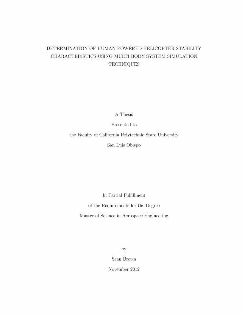
Vinci III[11]. Totah and Patterson modelled a tip mounted control system, that
deflects a blade section at each tip. The control system uses a linear control law
based on the differential tip height-to-ground sensed optically at each tip. Figure
1.8 show the tip-mounted control system. As an aside, the tip mounted control
system was recently implemented by NTS works Upturn, [33].
Figure 1.8: Tip-Mounted Control system for Da Vinci II[6]
Figure 1.9 shows the full Totah and Patterson model. Totah and Patterson
present response data for the control simulation showing a stable system. The Da
Vinci II model with a control system with rate and position limiting concluded to
be stable by Totah and Patterson. Totah and Patterson concluded the dynamic
9

model could not be validated due to the lack of available flight test data, and was
therefore considered preliminary.
Figure 1.9: Da Vinci configuration[6]
Guttieri’s report on the HPH stability and control was written after the Totah
and Patterson report. Guttieri derives the dynamics equations of the Da Vinci
from first principles and assesses the quasi-steady assumption for validity by
comparing the blade response when the quasi-steady assumption is used to the
response when it is not used. Guttieri concludes the quasi-steady assumption for
analysis of the dynamic response of the HPH is inappropriate. The conclusion
of Guttieri nullifies the conclusions of Totah and Patterson. There have been no
contributions to knowledge of the stability requirement for the human powered
helicopter problem.
The HPH problem has aerodynamics, structures and dynamic stability re-
quirements. Aerodynamics and structures have been treated in numerous reports.
The stability requirement of the HPH has not been treated, and cannot be easily
approached by traditional helicopter dynamics methods.
10
1.3 Solution
Traditional helicopter dynamic analysis builds the equations of motion from
the Newton-Euler equations. These non-linear equations are linearized for prelim-
inary analysis using several helicopter-specific assumptions([7, 34]). Traditional
linear stability theory is used to determine the stability of the linearized equa-
tions. The assumptions, however, must be applied with discretion. The helicopter
assumptions must be reassessed for validity if the configuration is altered or if
the vehicle operates in a different flight regime.
Multi-body system simulation(MBSSIM) is an alternate approach to deter-
mining the stability characteristics of helicopter configurations. Multi-body sys-
tem simulation is a discipline within Mechanical Engineering developed in the
1960s for treatment of complex satellite systems[35]. By the 1980s, computer soft-
ware was developed to allow for simulation and animation of these complex sys-
tems. Systems are broken into discrete rigid bodies with non-zero mass and iner-
tia. These bodies are then connected using joints to allow relative movement[36].
Forces and Moments are generated to set the system in motion through the use
of compliant elements. Research has been done using the multi-body systems ap-
proach in the field of Aeronautic and Machinery Design[37, 38], Biomechanics[39],
and Robotics[40]. Flexibility and reconfigurability are the major advantages
of MBSSIM. MBSSIM allow assumptions to be implemented by the designer,
through the development of discrete physics models. MBSSIM relies on numer-
ical integration, thus the stability of the system cannot be determined directly
from the system.
MBSSIM will produce the dynamic response of the system. System Identi-
fication is used to find a linear state space system from the dynamic response.
System identification is a field of control engineering whereby statistical meth-
ods are used to determine parameters of a mathematical model from a set of
measured data [41]. System identification can be used in any field where the re-
searcher requires a mathematical model to be produced from a data set. Specific
applications are found in aerospace and aeronautic [42]. System identification
11

will produce a discrete linear state space system. The stability properties of the
discrete linear state space system can be found through common linear stability
analysis theory.
This method solves the problem of determining the stability characteristics of
a human-powered helicopter, without the use of traditional helicopter dynamic
analysis. Figure 1.10 shows a information flow chart of the method developed
and implemented in this thesis.
12

User
Interface
MBSSIM
System Identification
Linear Stabil-
ity Analysis
Aero Model
Model Parameters
Processed Parameters
Time Response Data
State Space System
Eigenvalues
Stability
Power
Thrust
Figure 1.10: Multi-body Simulation Method
13

1.4 Thesis Scope
This thesis contribute to the knowledge of HPH stability through the de-
velopment of a method, which uses of multi-body system simulation, system
identification and linear stability analysis theory.
This thesis will present traditional helicopter dynamic theory. Presentation of
the traditional helicopter dynamic theory will be used to justify its abandonment.
This justification will focus on comparison of traditional helicopters and HPH
using non-dimensional terms important in rotor blade flap response. Helicopter
blade flap dynamics will be derived.
Combined Blade Element-Momentum theory is presented for use in modelling
the aerodynamics of the HPH. Combined Blade Element-Momentum theory dis-
cretizes a rotor blade into blade elements. The force acting at each blade element
will be a function of the local conditions. Momentum theory produces an equa-
tion for inflow which models the effects of the increase freestream velocity through
the rotor due to thrust.
This thesis will briefly discuss MBSSIM, system identification, and linear
stability analysis theory. MBSSIM uses first principle equations to automatically
generate equations of motion based on the discrete bodies and joints present in
the system. System identification finds parameters that will give a response that
matches the data set best, using probability techniques along with the equation
for the desired mathematical model. In this these the desired mathematical model
will be a discrete-time linear state space system of varying order. The system
identification section will treat system identification as a black box. The section
will only discuss the inputs and outputs to system identification and the options
available to the user. The solution to and stability of the discrete-time linear
state space equations will be discussed in the linear stability analysis section.
The stability analysis will present several theorem for determining the stability
of a linear system, but will not present proofs for them.
This thesis will discuss implementation of the HPH system into a commercial
MBSSIM Graphical User Interface(GUI), and the interfacing program used to
14

manipulate the GUI. MathWorks R© SimMechanics toolboxTM
is the MBSSIM used
in this thesis.
The interface to the MBSSIM GUI is developed in MathWorks R© MATLAB R©
for this thesis to allow for scripting of interactions with the MBSSIM. The in-
terface uses object-oriented programming techniques to control data access and
flow with the MBSSIM. The aerodynamic model is verified through a Richardson
extrapolation and an effort is made to validate it with experimental data from
UMD’s Gamera project. The experimental data used didn’t include experimental
uncertainty data, and thus the aerodynamic model will not be validated due to
insufficiencies in experimental data.
The results of this thesis present a demonstration of the method for dynamic
analysis of the Gamera quadrotor configuration. Time responses for the base
quadrotor configuration and the base quadrotor configuration with varied prop-
erties are presented. The stability properties identified through system identifica-
tion and linear stability analysis are presented. Parametric studies are presented
to demonstrate the methods use in a design capacity. The results show this
method of dynamics analysis can be used to determine the dynamic response and
stability properties of a HPH configuration. This work is only meant to discuss
tool development; and does not endorse any HPH design decisions.
1.5 Thesis Outline
Section 2.2 discusses traditional helicopter vehicle dynamics. This section will
also present a formal argument against the use of traditional helicopter dynamic
analysis. MBSSIM is be discussed in section 2.3. Rotor aerodynamic theory
will be presented in section 2.4. Next, the methods for system identification
and stability analysis will be discussed in sections 2.5 and 2.6, respectively. In
chapter 3, the specific implementation of MBSSIM will be discussed, along with
the verification and validation of the implemented aerodynamic model. Finally,
in Chapter 4, the author will demonstrate the abilities of this method. Section
15

2.1 will discuss the traditional helicopter and a comparison to the HPH.
16

Chapter 2
Theory
Helicopters produce required lift through the rotation of a lifting surface about
a locally vertical axis. Control of a helicopter is found through the cyclic or
collective change in the lifting surface pitch. The power required for lifting surface
rotation is produced from an on-board heat engine. The difference between HPHs
and traditional helicopters is the heat engine. HPHs have limited power and
endurance, compared to the traditional helicopter. This difference leads to a
branching of the design characteristics.
2.1 Helicopter Configurations
Traditional helicopter heat engines have a high power capability and enable
the production of a large amount of thrust via helicopter blades. The high power
capability creates a large design space for the traditional helicopter, with design
missions spanning cargo transport to high speed reconnaissance[43]. This large
design space allows the traditional helicopter to be designed to meet structure,
aerodynamic and dynamic stability requirements with a margin in each. Char-
acteristics for some traditional helicopters from, Padfield[34], are shown in Table
2.1. Figure 2.1 shows a traditional helicopter.
17

Figure 2.1: Lynx DRA Research Helicopter
2.1.1 The Human-Powered Helicopter Configuration
The power specification for a human, approximately 1 kW , confines the de-
sign space for a human-powered helicopter. Designers are driven to selecting
configurations that share the qualities of being light-weight, 55-100 lbs, and high
total wing spans, between 100-130 ft[44, 5]. For these reasons, the most successful
materials for HPH are carbon fiber composite, balsa wood, stiff foam, and some
type of shrink wrap film. Rotor blades are mostly empty with a carbon fiber
composite spar, wood or foam ribs and a shrink wrapped skin wing skin to make
and keep a smooth airfoil shape.
The four most common HPH designs are the coaxial rotor, tip propeller-
driven main rotor, a quadrotor, and the conventional main and tail rotor[5].
The quadrotor and the tip propeller-driven main rotor configurations will be
examined in this thesis due to their success. Characteristics for the Da Vinci
III and Gamera II, will utilized for the Quadrotor and tip-propeller driven main
18

rotor, respectively.
Table 2.1: Helicopter CharacteristicsCharacteristic Lynx Bo105 Puma Gamera I Da Vinci IIIRotor Radius, R(m) 6.4 4.91 7.5 6.5 20.42Rotation Speed, Ω(rad/s) 35.63 44.4 27 1.8 .6283Blades # (-) 4 4 4 2 2Kβ (Nm/rad) 166,352 113,330 48,149 – 74,167Lock Number,γ (-) 7.12 5.087 9.374 – 399.07Flap Frequency Ratio, λ2β 1.193 1.248 1.052 – 20.77
Power Loading (kg/kW ) 3.1916 3.9936 2.47 160 30.19Disk Loading (kg/m2) 105.3 91.25 103.2 1.2 .098Tip Reynold’s # (×105) 58.5 38.6 71.7 5-9 6
19

2.2 Helicopter Dynamics
We begin our discussion of helicopter dynamics with a quote to describe the
complexity taken on in helicopter dynamics analysis.
“...Not only is the aerodynamic environment of the rotor un-steady, but at the same time it is also non-linear, governed by non-infinitesimal motion and periodicity in conditions traditionally heldconstant with fixed wing applications...In addition to the problemsdirectly arising from unsteady aerodynamics those related to the factthat the rotor blades of contemporary helicopter rotors are ‘struc-tural lightweights’compared with their fixed wing counterparts. Theyachieve a large measure of their stiffening from the tension inducedby the rotational centrifugal force field. The rotational environmentof the rotor blades also give rise to a host of rotation-related phe-nomena: gyroscopic characteristics, Coriolis forces, and a variety ofnon-linear inertial loadings. While still governed principally by linearoperators, the resulting aeroelastic description of rotor blade elasticresponses is consequently fraught with non-linearities that modify theresult obtained using only linear analysis.”— Bielawa [45]
The main rotor will be the centerpiece of this discussion of helicopter dynam-
ics. Helicopter main rotor blades are designed to be flexible, in contrast to fixed
wing aircraft which are generally designed to be static. The degrees of freedom
for the blades of the main rotor are separated into out-of-plane rotation, in-plane
rotation about the vertical axis, and in-plane rotation about the span-wise axis,
which are known as flap, lag and feather, respectively. Figure 2.2 shows the rotor
degrees of freedom for a hinged rotor.
20

Figure 2.2: Hinged main rotor degrees of freedom, [7]
Traditional helicopters use the swash plate mechanism, shown in figure 2.3 to
change the feather degree of freedom in a collective or cyclic pattern, this is the
main control mechanism for a traditional helicopter
Figure 2.3: Helicopter Swashplate mechanism, [7]
A hingeless rotor is typical for most HPH and the degrees of freedom are
described the same but for the addition of elasticity in the blade response. Flap is
the focus of helicopter dynamics literature([7],[34]) in preliminary analysis phase.
Reassessment of helicopter dynamic analysis theory is required due to the dif-
ferences between a HPH and the traditional helicopter. Dynamic analysis for an
air vehicle involves the quantification and combination of the aerodynamic, struc-
tural and inertial responses. Furthermore, an individual set of equations must
be found for each helicopter configuration evaluated. The simplifying assump-
21

tions cannot be used in dynamic analysis if the components assumed negligible
are not. Each assumption must be evaluated to determine the difference in re-
sponses. The assumption can be used if the difference is negligible. Bramwell[7]
and Padfield[34] are referenced for all the material in this section.
2.2.1 Rigid Body Motion
This section will derive the equations for general translation and rotation of a
rigid body as a preface to the discussion of blade flap dynamics. Beginning with
the fundamental Newton equation,
F = mdv
dt(2.1)
Q =dh
dt= I
dΩ
dt(2.2)
, where Q is torque and F is force. The presence of rotational velocity requires
the use of
F = m(dv
dt+ Ω× v) (2.3)
, where Ω and v are the angular and linear velocities vectors respectively.
The components of force and torque acting on the body are
−→F = Xi+ Y j + Zk (2.4)
−→Q = Li+Mj +Nk (2.5)
The acceleration is expanded as,
22

ax = u− rv + qw − x(q2 + r2) + y(pq − r) + z(pr + q) (2.6)
ay = v − pw + ru− y(p2 + r2) + z(qr − p) + x(pq + r) (2.7)
az = w − qu− pv − z(p2 + r2) + x(pr − q) + y(qr + p) (2.8)
(2.9)
,where
−→a b = axi+ ay j + azk (2.10)
−→ω b = pi+ qj + rk (2.11)
−→r p/b = xi+ yj + zk (2.12)
.
The total force is found by integrating the force for every point on the body.
Assuming a body fixed coordinate system, B, at the center of mass, the differential
equations for linear motion of a rigid body is given as
X = Mb(u− rv + qw) (2.13)
Y = Mb(v − pw + ru) (2.14)
Z = Mb(w − qu+ pv) (2.15)
,where
v = ui+ vj + wk (2.16)
.
The derivation of the differential equations for rigid body rotational motion
can be found in [7]. The Euler equations, given off-diagonal terms present in the
inertia tensor, are
23

Ap− (B − C)qr +D(r2 − q2)− E(pq + r) + F (pr − q) = L (2.17)
Bq − (C − A)rp+ E(p2 − r2)− F (qr + p) +D(qp− r) = M (2.18)
Cr − (A−B)pq + F (q2 − p2)−D(rp+ q) + E(rq − p) = N (2.19)
.
A,B,C,D,E, F are components of the inertia tensor, and are used by
h1
h2
h3
=
A −F −E−F B −D−E −D C
ω1
ω2
ω3
(2.20)
,where
A =∑m(y2 + z2) B =
∑m(x2 + z2) C =
∑m(x2 + y2)
D =∑myz E =
∑mxz F =
∑mxy
(2.21)
.
The differential equations given in 2.13 through 2.15 and 2.17 through 2.19,
are the Newton-Euler equations and constitute a full set of differential equations
for rigid body motion. The rotational equations in Eq. 2.17 through Eq. 2.19
are used to present the flap degree of freedom.
2.2.2 Blade Flap
Analysis of Blade Flap begins by summing the moments due to inertial motion
and structural stiffness about the flap hinge to produce,
Kββ = −R∫
0
rm(r)(rβ + rΩ2β)dr (2.22)
.
24

The term Kβ is a measure of the blade hinge stiffness in the flap dof. The
inertial terms β and β on the right hand side, represent the force due to out-
of-plane flapping acceleration, and in-plane centrifugal acceleration, respectively.
This analysis make the assumption that there is no energy dissipation in the
structural response; in subsequent analyses this would be important to model,
but our discussion will diverge before this point.
The temporal differential equation is transitioned to a spatial differential equa-
tion by
ψ = Ωt (2.23)
d2
dt2= Ω2 d
2
dψ2(2.24)
.
The spatial differential equation is now
β′′ + λ2ββ = 0 (2.25)
,where λ2β is called the flap frequency ratio and is defined as,
λ2β = 1 +Kβ
IβΩ2(2.26)
.
The solution to the second order homogeneous differential equation 2.25 is
β = c1 cos(λβψ) + c2sin(λβψ) (2.27)
,where flap frequency ratio, λ2β, will define the undamped frequency of blade
flap.
The moments present at the flapping hinge must be reassessed when fuselage
pitch and roll velocity are added, because of the added angular velocity compo-
25

nents. The angular velocity components in the i, j, k coordinate system shown in
figure 2.4.
X
Z
Yp q
j
i
k
Ω
β
ψ
1
Figure 2.4: Flapping hinge coordinate system definition
For flapping and main rotor rotation only, angular velocity components of the
blade are
ω =
[Ω sin(β), −β, Ω cos(β)
](2.28)
.
Matrix equation form is used when generating the equations that account for
pitch and roll velocities; Angular components in matrix form are
ω = Rm(β)
(Rm(ψ)
−pq
0
+
0
0
Ω
)
+
0
−β0
(2.29)
, where Rm(ψ) and Rm(β) are rotation matrices about z-axis and the y-axis,
respectively.
26

The component accelerations are derived relative to the origin of the flap-
ping hinge. Euler equations are employed to produce blade flap dynamics. The
simplification by Padfield from the full differential is
β′′ + λ2ββ =2
Ω
(p cos(ψ)− q sin(ψ)
)(2.30)
.
In this equation it is assumed that rotor rotation speed is much greater than
the pitch and roll velocities; this assumption is usually valid for traditional heli-
copters.
Aerodynamic forces are added to the blade before solving the differential
equation. Effects of drag are negated and a two-dimensional lift model is used
for this analysis. The final flapping differential equation is
β′′ + λ2ββ =2
Ω
(p cos(ψ)− q sin(ψ)
)+
1
IβΩ2
R∫0
l(r, ψ)rdr (2.31)
, where
l(r, ψ) =1
2ρV 2ca0α (2.32)
.
θ, α, and φ are the geometric twist angle of attack and inflow angle, respec-
tively. The quantities, c and a0 are the chord length and the lift curve slope,
respectively. Figure 2.5 defines components of two-dimensional airfoil analysis.
27

x
y
X
Z
θ
L
D
V φ
α
Figure 2.5: Two Dimensional Aerodynamic Model
After simplification, the final flapping differential equation is
β′′ + λ2ββ =2
Ω
(p cos(ψ)− q sin(ψ)
)+γ
8
(θ − 4
3λi +
p
Ωsin(ψ)
q
Ωcos(ψ)
)(2.33)
,where λi and γ are the inflow ratio and Lock number, respectively. The lock
number is defined as
γ =ρca0R
4
Iβ(2.34)
.
λi and θ are the inflow ratio and blade pitch respectively; blade pitch is
assumed to be a sinusoidal function of ψ and is traditionally based on pilot
control. The differential equation is solved using quasi-steady assumption.
The goal of this discussion is to check if the quasi-steady assumption is valid
for the HPH configuration. This assumption may be used if the rotor reaction
28
to a single control input is an order of magnitude faster than the change in the
fuselage angular velocity or pilot control; it will allow the decoupling of the main
rotor and fuselage dynamics.
The Lock number and Flap Frequency Ratio, γ and λ2β, are used to determine
if the quasi-steady assumption can be applied. These numbers represent the
ratio of aerodynamic to inertial forces, and the ratio of structural to inertial
forces, respectively. Table 2.1 shows the Lock number and flap frequency ratio
for three traditional helicopters and the Da Vinci HPH; aerodynamic forces are
greater than the inertial forces for all the helicopters presented. Notice that
the HPH Lock number is 57 times greater than the average Lock number for
the traditional helicopter. The flap frequency ratio is 18 times greater than the
average flap frequency ratio for the traditional helicopter. The previous two facts
imply that the aerodynamic and structural dynamic responses is much greater
than the inertial response for the Da Vinci HPH.
Assessment of the goals for past HPH project teams makes this clear concep-
tually. The goal for past HPH projects is to build the vehicle bigger, lighter and
stronger. The strength in the rotor blade spars and other structure will increase
the flap frequency ratio. The Lock number will be increase as the rotor blades
become bigger without a equivalent increase in blade weight.
Guttieri[32] concludes the response time for a disturbed Da Vinci rotor blade
in flap is greater than 3 seconds. The change in fuselage angular velocity is not
an order of magnitude slower than the change in rotor flap angular velocity, and
thus the quasi-steady assumption cannot be used.
Totah[6] found, through simulation, the maximum pitch velocity is approx-
imately 0.45 rad/sec. The design rotation speed of the Da Vinci main rotor is
approximately 0.63 rad/sec. The rotor rotation speed was assumed to be an
order of magnitude faster than the pitch velocity of the fuselage. This is not the
case for HPH configurations, thus the assumption is not valid for the HPH.
The quasi-steady assumption and the rotation speed assumption will not be
valid for the HPH. The equations will have to be re-derived by including previ-
29

ously negated terms to continue with this line helicopter dynamic analysis. The
absence of experimental data will not allow for validation of the newly generated
dynamic equation. The use of traditional helicopter dynamic analysis is discour-
aged by number of terms that must be re-evaluated for importance. Multi-body
system simulation is chosen instead, due to the ability to fully treat the coupling
between the rotor blades and the fuselage and its simple implementation.
2.3 Multi-Body System Simulation
Multi-body systems simulations are built from basic dynamics. The method
can generate and simulate the equations for an arbitrary number of bodies and
joints. The equations are generated in the form most easily manipulated for nu-
merical integration, not the minimal representation used by analytical dynamic
analysis. Von Schwerin[36] discusses in-depth the advantages of matching the
structure of the dynamics equations to the numerical solver. These options in-
clude changing the coordinate system, the variables used and the formalism of
numeric vs symbolic. Theory of multi-body system simulation will be considered
beyond the scope of this thesis. MathWork’s SimMechanics is the multi-body
system simulator used. MBSSIM requires models for all physics beyond body
dynamics and gravity. This required development of an aerodynamic model.
2.4 Aerodynamic Model
A discrete aerodynamic model was developed to account for the aerodynamic
effects experienced by helicopter rotor blades. Different aerodynamic models will
be discussed first. Each model can be used to simulate a different aerodynamic
effects. The chosen aerodynamic model will be discussed in-depth.
Momentum theory[46] is the simplest method. Momentum theory uses the
actuator disk assumption and the principle of conservation of momentum to cal-
culate the power for a given thrust. This is a one-dimensional method and doesn’t
30

account for variation in span-wise blade parameters or a complex rotor wake en-
vironment.
The second method is blade element theory, which discretizes a rotor blade
and integrates the lift and drag over the entire blade based on the local blade
element conditions. The span-wise airfoil geometry can be varied at each blade
element. Classical implementation of the method achieves a commanded thrust
by iterating on geometric twist/pitch. Empirical inflow equations are used to
model the effects of flow through the rotor as a function of thrust. Ground effect
is implemented in blade element theory by altering the local span-wise or global
power due to induced drag.
These two method are combined to create a third aerodynamic model. Com-
bined Blade element-momentum theory uses momentum theory to model inflow
effects. It can still model non-constant span-wise airfoil geometry. Combined
blade element-momentum theory(BEMT) rotor aerodynamic analysis will be used
in the work presented below, due to its ease of implementation and validated
results[17]. BEMT cannot model complex wake effects, such as, trailing tip vor-
tices.
Vortex methods use discrete vortex filaments that trail from the rotor blade
to mimic complex airflows present in the rotor wake. Gilad applied prescribed
wake vortex method to the HPH rotors. Gilad concluded vortex methods don’t
produce results that are significantly more accurate than BEMT to justify the
added time in the preliminary design phase.
Computational fluid dynamics(CFD) simulations are the most complex set of
modelling techniques. CFD can model very complex free wake effect in the near
and far-field. CFD does require a significant amount of computation resources
to implement, and validate. CFD is too expensive for this stage of the HPH
design[47]. BEMT is chosen as the aerodynamic model used for simulation of the
dynamics of the HPH in a multi-body system simulation. The methodology for
determining the aerodynamic forces in the MBSSIM are presented in the next
section.
31

2.4.1 Methodology
MBSSIM discretizes a vehicle body into a finite number of elements, which is
used for implementation of the BEMT model. This aerodynamic model formu-
lation can be found in Leishman[46], Bramwell[7], Padfield[34], or Johnson[43].
Blade element properties, local linear and angular velocity and the linear
displacement from the ground are the inputs to the aerodynamic model. The
aerodynamic model will calculate the resultant aerodynamic forces in the local
blade element coordinate system.
Lift curve slope, parasite drag coefficient, chord length, reference area, and
pitch angle are the local blade properties required for each element. Blade radius,
and the total number of blades are global rotor properties required for each
element.
A solution requires fixed point iteration on pitch to achieve the commanded
thrust in traditional formulation of BEMT. Pitch/geometric twist angle is com-
manded at each span-wise location, making thrust and power an output in the
MBSSIM formulation. This method is similar to experimental procedure rather
than computer simulation. The inflow velocity is calculated using the inflow ratio
defined as
λ =vi
ΩR(2.35)
.
The inflow ratio calculation is described in section 2.4.2. The inflow velocity
and the vehicle vertical velocity are used to find the local vertical velocity at the
blade element, shown as
UP = λ(r)ΩR + Vc (2.36)
.
The local horizontal velocity is an input to the aerodynamic model imple-
mented in MBSSIM. The local horizontal velocity for a rotor in hover is calculated
as
32

UT = ΩR(r) (2.37)
.
Sideslip forces are generated from velocity in the span-wise direction. Sideslip
forces are assumed to have little or no effect. Sideslip velocity is used in calcula-
tion of velocity magnitude,
U =√U2T + U2
R + U2P (2.38)
.
The inflow angle is calculated as
φ = tan−1(UPUT
) (2.39)
.
The inflow angle is used to determine the local angle of attack of the rotor
blade by
α = θ − φ (2.40)
.
The coefficient of lift and drag are calculated and dimensionalized to give the
forces in the wind axes in equations 2.41 through 2.43. The lift and drag forces
act perpendicular and parallel to the velocity vector, respectively.
Cl = Clαα (2.41)
L =1
2ρU2SCl (2.42)
D =1
2ρU2SCd (2.43)
The method for calculation of the drag coefficient requires more detailed ex-
planation. Assuming a drag polar equation is the simplest method for drag
33

coefficient calculation. A common form is
Cd = Cdo +KC2l (2.44)
.
The coefficients, K and Cdo, are the induced drag coefficient and the parasite
drag coefficient, respectively. A common empirical equation for K is
K =1
πeAR(2.45)
.
Interpolated aerodynamic tables are the second method for calculating drag
coefficient. Numerical or experimental data is used to generate the aerodynamic
tables. The tables can be interpolated using the local coefficient of lift or angle
of attack and Reynold’s number. The drag polar equation was used in this
implementation of the aerodynamic model. The value of Cdo is calculated by
averaging the zero-lift drag coefficient over the proper range of Reynolds numbers.
MBS simulation requires force input in the local body reference coordinate
system. The local body coordinate system x-direction points in-plane upstream,
the z-direction points perpendicular to the disc plane, and the y-direction makes
an orthogonal coordinate system. The coordinate system is shown in figure 2.5.
The positive z-direction is defined as away from the ground reference. The rota-
tion of the forces from the wind axes into the local body frame is done using a
rotation matrix.
Select configurations of the HPH require both counter-rotating and forward
rotating rotors. This needs to be explicitly accounted for in the MBSSIM aero-
dynamic model. The linear and angular velocity are assumed positive. If both
are negative, a signal will be sent to the rotation matrix to change the rotation
such that the drag is always acting in the direction opposite the body velocity.
34
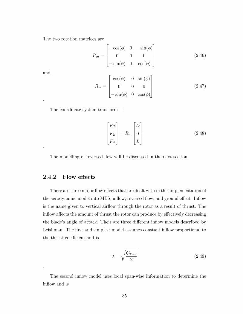
The two rotation matrices are
Rm =
− cos(φ) 0 − sin(φ)
0 0 0
− sin(φ) 0 cos(φ)
(2.46)
and
Rm =
cos(φ) 0 sin(φ)
0 0 0
− sin(φ) 0 cos(φ)
(2.47)
.
The coordinate system transform is
Fx
Fy
Fz
= Rm
D
0
L
(2.48)
.
The modelling of reversed flow will be discussed in the next section.
2.4.2 Flow effects
There are three major flow effects that are dealt with in this implementation of
the aerodynamic model into MBS, inflow, reversed flow, and ground effect. Inflow
is the name given to vertical airflow through the rotor as a result of thrust. The
inflow affects the amount of thrust the rotor can produce by effectively decreasing
the blade’s angle of attack. Their are three different inflow models described by
Leishman. The first and simplest model assumes constant inflow proportional to
the thrust coefficient and is
λ =
√CTreq
2(2.49)
.
The second inflow model uses local span-wise information to determine the
inflow and is
35
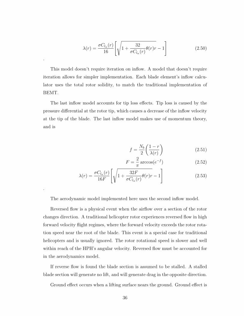
λ(r) =σClα(r)
16
[√1 +
32
σClα(r)θ(r)r − 1
](2.50)
.
This model doesn’t require iteration on inflow. A model that doesn’t require
iteration allows for simpler implementation. Each blade element’s inflow calcu-
lator uses the total rotor solidity, to match the traditional implementation of
BEMT.
The last inflow model accounts for tip loss effects. Tip loss is caused by the
pressure differential at the rotor tip, which causes a decrease of the inflow velocity
at the tip of the blade. The last inflow model makes use of momentum theory,
and is
f =Nb
2
(1− rλ(r)
)(2.51)
F =2
πarccos(e−f ) (2.52)
λ(r) =σClα(r)
16F
[√1 +
32F
σClα(r)θ(r)r − 1
](2.53)
.
The aerodynamic model implemented here uses the second inflow model.
Reversed flow is a physical event when the airflow over a section of the rotor
changes direction. A traditional helicopter rotor experiences reversed flow in high
forward velocity flight regimes, where the forward velocity exceeds the rotor rota-
tion speed near the root of the blade. This event is a special case for traditional
helicopters and is usually ignored. The rotor rotational speed is slower and well
within reach of the HPH’s angular velocity. Reversed flow must be accounted for
in the aerodynamics model.
If reverse flow is found the blade section is assumed to be stalled. A stalled
blade section will generate no lift, and will generate drag in the opposite direction.
Ground effect occurs when a lifting surface nears the ground. Ground effect is
36

modelled by a proportional decrease in the induced power required for a constant
thrust. Ground effect is experienced by both non-rotating and rotating lifting
surfaces. Traditional helicopter experimental data regarding ground effect is not
in the proper flight regime for the HPH. The ground effect coefficient is defined
as
kG =PIGEPOGE
(2.54)
.
This ground effect coefficient is applied per-radial station to the inflow ratio,
λIGE(r) = kG(r)λOGE(r) (2.55)
The ground effect coefficient data is traditionally plotted against the distance
from the ground non-dimensionalized by the rotor radius, or zR
. The minimum
value of zR
for traditional helicopters is 0.46 to 0.61. This contrasts with the
maximum value for a HPH of 0.46. Traditional ground effect experimental data
or analytical equations are not valid for the purposes of this aerodynamic model.
University of Maryland’s(UMD) Gamera project generated experimental data
for ground effect in the proper flight regime. The experiment used the UMDs
ground effect test rig (GETR), discussed in [17], [48], and [49]. The GETR is
a 1.37 m sub-scale test rotor which is moved translated vertically from a z/R
value of 2 to .1. The thrust from the rotor and the power required by the motor
were recorded. A curve fit is applied to the ground effect coefficient data. Ground
effect becomes negligible as the rotor gets further from the ground, so a horizontal
asymptotic function was chosen for the curve fit. The horizontal asymptote for
kG is 1 as the height ratio goes to positive infinity. The data shows that the
ground effect factor becomes negligible at a height ratio of 2. This experimental
data and the curve fit are shown in figure 2.6.
37

0 0.5 1 1.5 2 2.50.2
0.3
0.4
0.5
0.6
0.7
0.8
0.9
1
1.1
1.2
TrendlineGETR Exp
Figure 2.6: Ground Effect Data from UMD along with the correspond-ing trendline
The theory behind the aerodynamic model has now been presented. The
model will be verified and validated in section 3.4.
2.5 System Identification
System identification will be used to generate a linear state space model. The
inner workings of system identification and its associated methods are discussed in
detail in Van Overschee[41]. System identification will be treated as a black box in
this thesis. The input form, options available to the user and, the form and quality
of the output will be discussed. System identification is the process of using
time response data from a simulation to generate a mathematical model. The
implementation of system identification using a commercial computer program
will be described in chapter 3.
The time dependent dynamic states of the system are referred to as the output.
The state space model that is product of system identification is referred to as
the identified model. The time-dependent data that is used as an input to the
38

system is referred to as the input data. The instantiated object fed into the
system identification function is referred to as the input object.
Numerical integration algorithms use adaptive time stepping to resolve areas
with larger derivative. Uniform time step interpolation must be performed to
make a uniform time step over the data set. Uniform time step is a requirement
of the specific system identification algorithm. The time response data is assumed
to be of sufficient resolution to apply a linear interpolation without any loss of
data characteristics.
2.6 Stability
System identification was used to generate a linear state space model such that
the vast literature surrounding linear system stability can be brought to bear on
the problem[50]. The stability of the system can be evaluated through linear
stability analysis theory. This section begins with a discussion of the solution to
the linear state space system. The definition of stability will then be discussed.
Finally, the types of stability and indications of stability will be discussed.
The identified system is a linear discrete-time state space system. The current
state vector x(k) is
k = ko : x(k + 1) = A(k)xk +B(k)u(k)
k = ko + 1 : x(k + 1) = A(k)xk +B(k)u(k)
= A(ko + 1)A(ko)xo + A(ko + 1)B(ko)u(ko)+
B(ko + 1)u(ko + 1)
k = ko + 2 : x(k + 1) = A(k)xk +B(k)u(k)...
......
(2.56)
Using inspection, the solution reduces to
39

x(k) = Akxo +k−1∑j=0
AjBu(k − j − 1) (2.57)
, if the system is time-invariant.
The complete solution, y(k), is
y(k) =
Cxo +Du(ko) , k = ko
CAkxo +k−1∑j=0
CAk−j−1Bu(j) +Du(k) , k ≥ ko + 1(2.58)
.
Rugh[50] defines stability as involving the boundedness properties and asymp-
totic behavior of a system. Linear systems can either be classified as exponentially
stable, or unstable. The proof for stability and all involved theorems will not be
presented in this thesis.
A system is exponentially stability, if there exist a finite positive constant γ
and a constant 0 ≤ λ ≤ 1 such that for any ko and xo the solution presented
above satisfies
||x(k)|| ≤ γλk−ko ||xo||, for k ≥ ko (2.59)
.
This definition can be applied to the state equations, without assessing the
solution to the state equations, through the calculation of the eigenvalues. The
eigenvalues are calculated for the discrete time case through a z-transform on the
zero-input state equation and are the roots of
Z[Ak] = z(zI − A) =z · adj(zI − A)
|zI − A|(2.60)
.
A linear time invariant state equation is exponentially stable if and only if
all eigenvalues of A have magnitude strictly less than 1, is the key result. If this
40

condition is not satisfied, the solution will identified by default as unstable. In
the unstable case the solution is assumed to grow without bounds.
2.7 Summary
The theory used in this thesis is presented in this chapter. The Newton-
Euler equations are presented to begin the presentation of traditional helicopter
dynamic analysis. The traditional helicopter dynamic analysis focuses on the
dynamic of the main rotor, specifically the flap degree of freedom. Equations of
motion for the flap degree of freedom are derived with aerodynamic, structural
and fuselage motion effects. The quasi-steady assumption is applied to decouple
the rotor and fuselage interaction. The quasi-steady assumption cannot be ap-
plied to the HPH due to similarity in fuselage and rotor response times. This
breakdown creates the need for a different method for HPH dynamic analysis.
This alternate method is chosen to be Multi-Body System Simulation.
MBSSIM uses a set of bodies and joints to automatically generate the equa-
tions of motion for a system. These equations of motion can then be numerically
integrated to generate a time response for the system. MBSSIM requires models
for all physics beyond body dynamics and gravity. This required development of
an aerodynamic model. The theory for the aerodynamic model is presented in
this chapter.
MBSSIM and aerodynamic theory are used to generate dynamic time response
data. The time response data is processed and used for system identification.
System identification generates a linear discrete time state space equation. The
linear discrete time state space system is found to be to be stable or unstable
thus identifying the time response data as stable or unstable. The method for
determining the stability of a linear discrete state space system is presented in
this chapter .
41

Chapter 3
Implementation
The implementation of the models is explained here. Simulink R© is a GUI,
which uses blocks to represent mathematical processes applied to a time depen-
dent signal. The SimMechanics toolboxTM
adds the ability to perform multi-body
system simulations to Simulink. An example of implementation of a simple phys-
ical model will be discussed to better introduce the reader to MBSSIM. A set of
object classes used to add scripting to the MBSSIM functionality were develop
for the HPH application.
The implementation of the aerodynamic model is presented in this chapter.
The aerodynamic model is verified by comparing rotor performance for a single
flight condition using a varying number of elements. The specific method used
for verification is a Richardson Extrapolation. The Richardson Extrapolation
determines the numerical uncertainty by calculating the error in the model based
on the change in performance for a varying numbers of elements. The Richard-
son Extrapolation calculates the apparent order of the aerodynamic model. An
effort is made to validate the implemented aerodynamic model. The validation
compares experimental data to the numerical data for equal flight conditions.
42

3.1 SimMechanics Implementation
The SimMechanics block set contains basic bodies, joints, sensor and actua-
tors. The body block holds user-defined mass and inertia properties. The user
can define the coordinate system orientation and position. The body block can
have any number of coordinate systems and can be at any orientation or distance
from the coordinate system attached to the previous joint. The center of gravity
position and orientation can be defined. The orientation of a coordinate system
can be set through a set of Euler angles, a 3-by-3 orthogonal rotation matrix, or
a 1-by-4 row vector quaternions. Joints blocks hold user-defined degrees of free-
dom. Rotation and translation are the two types of degrees of freedom. Joints
can have a maximum of 6 degrees of freedom, 3 translation and 3 rotation. The
basic body and joint block type can be copied and combined to create any phys-
ical mechanism. A body cannot be attached to another body and a joint cannot
be attached to another joint. Systems can be modelled in a generalized way, or
in detail depending on the level of analysis or design.
Compliant elements create motion in the system. The actuator block is the
basic form of the SimMechanics compliant element. The input of a actuator
block is a Simulink signal, and the output is connected to a joint or body. The
body actuator block induces motion in the body through force or moments. The
joint actuator block induces motion in the joint through forces, moments or the
prescription of motion. The prescription of motion requires the position, velocity
and acceleration of each degree of freedom actuated. Prescribed motion does not
generate a reaction force or moment to counteract the motion. Prescribed motion
will not be used in the simulation of a HPH due to the lack of reaction forces or
moments.
The sensor block is the fourth major block type. The sensor block can be used
to measure the states of a joint or body. The body sensor can measure twenty-four
states, linear position, linear velocity, linear acceleration, nine element rotation
matrix, angular velocity, and angular acceleration. These states can be measured
in the absolute coordinate system, or in the local coordinate system in which
43

the sensor is attached. The joint sensor can measure the position, velocity and
acceleration for each joint degree of freedom. The joint sensor can measure the
reaction forces or moment over the joint. Closed loops can be develop through
the use of a sensor and actuator block.
Sensors and actuator block output and input a Simulink signal, respectively.
The Simulink signal can be displayed or analysed by the user using several types
of output blocks. The model can be simulated to produce the time response of
the configuration. This multi-body system approach to modelling complex be-
havior of bodies allows a reduction in the designers time spent in understanding
and modelling of complex helicopter dynamics. This is appropriate for the HPH
project. The downside of MBSSIM and numerical time integration is the absence
of explanation for couplings. There is no equation that can be checked to deter-
mine the strength or weakness of components of the dynamic response. Sensors
can be used to mitigate this downside through reaction force and torque sensing.
A sensor is attached to the rotor rotational joint to sense the reaction forces
and torques across the rotor joint. These reaction forces and torques are used to
calculate the power required and thrust generated.
Simulink allows the development of custom block libraries, that when used in
a model, are still linked to the original library block. This link can be used to
push or pull changes from or to the original library block. This feature allows
for modularization and discretization. Documentation and discussion of the best
practices in SimMechanics can be found in Appendix A.
Before continuing to the next section, a small example will be presented to
better introduce the reader to MBSSIM. This example models a double pendulum
and is taken from MathWorks([8]). The double pendulum can be described as
having to two unique parts. First, the bar has some mass, inertia and length, and
second is the joint which determines around which axis the bar can rotate. Figure
3.1 shows a simple drawing a double pendulum with the described elements.
44

Figure 3.1: Double Pendulum Drawing[8]
These two elements of the double pendulum are described in SimMechanics
as a body block and a revolute joint block. Figure 3.2 shows a SimMechanics
model of the double pendulum. The red blocks represent revolute joints, and
the blue blocks represent the mass and length of each aspect of the pendulum.
The green block represents the fixed surface to which the double pendulum is
attached. Sensor blocks and initial condition blocks are included in this model.
This model can now be simulated and the system time response determined.
45

Figure 3.2: Double Pendulum Model[8]
The example above demonstrates how a physical system can be simplified
and modelled in SimMechanics. This same method is used to develop the HPH
models used in this thesis.
3.2 Text User Interface
Properties must be changed manually in normal SimMechanics modelling.
The GUI aspect of SimMechanics is efficient for development of multi-body sys-
tems. SimMechanics is unable to script changes to the model. The text user
interface developed for this thesis enables the scripting of SimMechanics model
property changes and the recording of the time response results. This interfacing
will enable the MBS to be used in design tools, such as parameter sweeps.
The text user interface is a set of object classes, which are attached to different
components of the multi-body system. The Model Discovery class, and Block
46

Parameter class are the two main types of object classes in the text user interface.
The block parameter class contains all information about the properties of each
block in the model.
Objects are instantiated and attached to specific Simulink model blocks. The
attached objects query the model block for specific parameters and populate the
corresponding object properties. The object and the model block are now linked,
such that when a object property value is altered, the corresponding model block
parameter is altered. Each block parameter object property has access methods
that will control the data types and values sent to the model blocks. This is
a safeguard against a common source of simulation error. The block parameter
objects are sub-classed due to variation in model block parameters.
A Model Discovery class object is instantiated for each SimMechanics model
that is generated. The Model Discovery object has properties linked to global
model parameters. A Model Discovery object has properties that contain the
figures of merit, scope data and identified system data. The Model Discovery ob-
ject also contains handles for the block parameter class objects. Model Discovery
class methods are used to simulate the model, process the model time response
and input/output groups of model parameters.
Figure 3.3 shows a block diagram of the parameter classes and subclasses,
along with their unique properties.
47

Block
Para
meters
Pro
per
ties
Blo
cknam
eT
yp
eM
odel
ModelDiscovery
Pro
per
ties
Model
Para
met
erO
bje
ctlist
Blo
ckN
ames
Sco
pe
dat
aF
igure
sof
Mer
itG
ravit
yL
iste
ner
han
dle
s
Met
hods
Dis
cover
Sim
Model
Gen
erat
ePlo
tsP
ara
met
erG
enP
ara
met
erV
ecIN
Para
met
erV
ecO
UT
BodyPara
meters
Pro
per
ties
Mas
sIn
erti
aC
GP
osi
tion
CS
Posi
tion
CS
Rot
atio
n
Actu
ato
rPara
meters
Pro
per
ties
Rot
atio
nSp
eed
Sig
nal
Typ
eD
OF
Axis
Chir
pF
requen
cyC
hir
pG
ain
Roto
rPara
meters
Pro
per
ties
Num
ber
ofB
lades
Ele
men
tM
ass
Ele
men
tIn
erti
aC
hor
dP
itch
Lif
tC
urv
eSlo
pe
Par
asit
eD
rag
Coeff
Rad
ius
CarrierPara
meters
Figure 3.3: Class Diagram
48

3.3 System Identification
The system identification toolboxTM
in MATLAB R© is used to perform system
identification through the n4sid function. This function requires the input of an
iddata object, which contains time, input and output data, and the order of the
identified model. The form of the identified state space model is
x(k + 1) = Ax(k) +Bu(k) (3.1)
y(k + 1) = Cx(k) +Du(k) (3.2)
.
The A,B,C,D matrix sizes are determined by the order of the model, number
of inputs, and outputs. If n is the model order, m is the number of system inputs,
and l is the number of system outputs, A is n× n, B is n×m, C is l× n, and D
is l ×m. The number of parameters available to the system identification algo-
rithm is set when the model order chosen. The system identification toolboxTM
implemented in MATLAB R©, has a assessment and recommendation system for
choosing the model order. The user is referred to the MathWorks documentation
for more details[51].
3.4 Aerodynamic Model
In section 2.4, the theory behind the aerodynamic model was discussed. The
implementation of the theory into SimMechanics is discussed in this section. The
implemented model solution will be verified and validated to be accurate enough
for our purposes. Code verification takes the form of debugging and error checking
and will not be discussed. Solution verification has three aspects, input accuracy,
numerical solution accuracy, and output data accuracy. Numerical solution accu-
racy will be the only aspect discussed. Validation studies measure the amount of
agreement between computational results and experimental measurements. The
49

theory and methods behind verification and validation studies are discussed in
detail in Oberkampf[52].
The aerodynamic theory implementation is shown in figure 3.4. This model
represents a feedback system meant to actuate a body element. This body ele-
ment will be actuated to simulate a lifting surface element in a rotor blade.
50

Fwin
d
5
Zout4
q3
Lam
bda
2
y11
Act
uato
r
2
Sen
sor
1
0
Zero
1
[0;0
;0]
Vel
ocity
mod
ifica
tion
Z Vin
Om
ega
Cla
Thet
a
y
Vou
t
Lam
bda
Zout
Forw
ardF
low
UY
Sel
ecto
r1
UY
UY
Rot
Mat
Mod
phi
Om
ega
Rot
atio
n
R_n
el
R/n
el
Pro
duct
4
Mat
rixM
ultip
ly
Got
o3
[For
ces]
Got
o2
[The
ta]
Got
o1
[Cla
]
Got
o
[Cha
r]
From
3
[For
ces]
From
2
[The
ta]
From
1
[Cla
]
From
[Cha
r]
Div
ide
Cha
rPic
k
Inde
xC
har
Bod
y S
enso
r
p v av
Bod
y A
ctua
tor
Ang
leW
Forc
es
V thet
a
Cha
r
Forw
ardF
low
dD dL q
Phi
y1
Z
Inde
x
thet
a
Figure 3.4: Aerodynamic model implemented in Simulink
51

3.4.1 Verification
Numerical error estimation is the focus of the verification section. Estimation
of numerical error is determined using the order of accuracy through refinement
of the finite element method used in SimMechanics. A SimMechanics rotor is
modelled and simulated with a varying number of body elements to assess the
change in a global parameter, Power coefficient(CP ). The parameter is assumed to
converge to a value absent of numerical error as the number of elements increases
toward positive infinity. Figure 3.5 exhibits this convergence.
10 15 20 25 30 35 40 451.158
1.159
1.16
1.161
1.162
1.163
1.164
1.165
1.166x 10
−4
Number of Elements
CP
Figure 3.5: Grid Refinement Study for Aerodynamic model on repre-sentative rotor
An a posteriori error estimation was performed using the grid refinement study
data to determine the observed order of the system and the estimated numerical
error the figure of merit[53]. Richardson extrapolation is the specific a posteriori
error estimation used. The results of this study are summarized in Table 3.1
below. Apparent order, extrapolated error, and GCI are the important figures
to note. The apparent order for this study is 2nd order, indicating quadratic
52

Table 3.1: Discretization Error: Richardson ExtrapolationAttribute Cp
Number of element, (N1, N2, N3) 45,30,10Grid refinement factor, r21 1.5Grid refinement factor, r32 3C1p 0.11641× 10⁻³
C2p 0.11638× 10⁻³
C3p 0.11586× 10⁻³
Apparent order, p 2.0001C21p ext 0.4659× 10⁻⁴
Approximate Relative Error, e21a 0.31134× 10⁻²%Extrapolated relative Error, e21ext 149.8%Fine-grid convergence index, GCI21fine 3.1132× 10⁻²%
convergence. The extrapolated relative error is a measure of the relative error
when the number of elements approaches infinity. The extrapolated relative error
for the finest mesh is approximately 150%. This is due to the relatively low
number of elements used when compared to the order of magnitude of the power
coefficient. The grid convergence index(GCI) is the ratio of the approximate
relative error to the grid refinement.
Verification study indicates that the numerical uncertainty is sufficiently low
when using ten elements. Ten elements will be used in the rotor validation studies
and in all models used in the results section.
3.4.2 Validation
The aerodynamic model needs to be validated to predict realistic trends and
effects, now that the model has been verified. The validation study will compare a
numerical rotor model and attached aerodynamic model with experimental data
of helicopter rotor. The experimental data needs to have dynamic similarity with
the complete system that the tool will be applied to.
Dynamic Similarity is established by matching the Reynold’s numbers at the
tip of the rotor blade. Reynold’s number is given by
53

RE =V c
µ(3.3)
, where µ is the kinematic viscosity, and is assumed to be 1.5236 × 10⁻⁵m2
sec.
Table 2.1 details the Tip Reynold’s number ranges for the historical HPHs. The
validation data selected to match these ranges comes from the University of
Maryland(UMD), where the recent development of the Gamera has produced a
large amount of experimental data on low-Reynolds number rotor performance.
Table 3.2: Experimental Test DescriptionAttribute UMD GETR UMD FSTR
Radius (m) 1.37 6.5Chord (m) .27 1Twist none noneTaper none noneReynolds Number Range(×105) 1.37-2 5-9Airfoil NACA 0012 Eppler 387
The two experimental setups used for validation data are the sub-scale ground
effect test rig(GETR), and the full scale HPH blade test rig(FSTR), which ap-
pear in [17] and [49]. The UMD Full Scale test rig experiences ground effect,
and for this reason the GETR was included to validate the aerodynamic model
out-of-ground effect(OGE). Table 3.2 lists the characteristics for each experimen-
tal setup. A SimMechanics model was built with specifications for each UMD
experimental setup used to record the validation data.
Figures 3.6 through 3.9 show comparison of the SimMechanics aerodynamic
model and GETR experimental with a variation of rotor rotation speed. Figures
3.10 and 3.11 show a comparison of the SimMechanics model and the Full scale
test rig with variation in rotor height above ground. The dashed line in each
figure represents the numerical aerodynamic model results from Gilad[17], and
are presented for comparison.
The SimMechanics Model in figure 3.6, shows good correlation with the ex-
perimental data and numerical simulation performed by Gilad. The last data
point in the figure shows the start of stall as a higher thrust is commanded. The
54

SimMechanics model did not account for stall at high angles of attack. The Sim-
Mechanics model consistently over-predicts the coefficient of power compared to
Gilad’s numerical simulation.
0 0.002 0.004 0.006 0.008 0.01 0.0120
0.2
0.4
0.6
0.8
1
1.2
1.4
1.6
1.8
2x 10
−3
CT
CP
GETR Exp
Gilad Aero Model
SimMechanics
Figure 3.6: SimMechanics Validation using UMD GETR data Ω =54rpm z/R = 2
Figure 3.7 shows slightly better correlation between the experimental data
and the SimMechanics model. The SimMechanics model still over-predicts the
coefficient of power compared to Gilad’s numerical simulation.
55

0 0.002 0.004 0.006 0.008 0.01 0.0120
0.2
0.4
0.6
0.8
1
1.2
1.4
1.6
1.8x 10
−3
GETR Exp
Gilad Aero Model
SimMechanics
Figure 3.7: SimMechanics Validation using UMD GETR data Ω =66rpm z/R = 2
Figure 3.8 an under-prediction of the coefficient of power compared to the
experimental data. The SimMechanics model, again, shows an over-prediction
compared to Gilad’s numerical simulation.
56

0 0.002 0.004 0.006 0.008 0.01 0.0120
0.2
0.4
0.6
0.8
1
1.2
1.4
1.6x 10
−3
Exp
Gilad Aero Model
SimMechanics
Figure 3.8: SimMechanics Validation using UMD GETR data Ω =78rpm z/R = 2
Figure 3.9 shows the SimMechanics model agains the experimental data pub-
lished by the UMD. This data is taken at 82 RPM, which corresponds to a
Reynolds number of 2.08× 10⁵. The SimMechanics model under-predicts the co-
efficient of power compared to the experimental data. The SimMechanics model
over-predicts the coefficient of power compared to Gilad’s numerical simulation.
57

0 0.002 0.004 0.006 0.008 0.01 0.0120
0.2
0.4
0.6
0.8
1
1.2
1.4
1.6
1.8
2x 10
−3
CT
CP
Exp Gilad Aero ModelSimMechanics
Figure 3.9: SimMechanics Validation using UMD GETR data Ω =82 rpm z/R = 2
Figure 3.10 shows the SimMechanics rotor model compared to the experimen-
tal data collected from the UMD’s full scale test rig. The experimental data was
collected at a Reynolds number of 8.04×10⁵ and a height ratio of .1 The SimMe-
chanics rotor model over-predicts the coefficient of power at coefficients of thrust
between 0.005 and 0.007 compared to the experimental data. The SimMechanics
model has low error when compared to the experimental at coefficient of thrust
numbers above 0.008.
58

0 0.005 0.01 0.0151
2
3
4
5
6
7
8
9
10x 10
−4
CT
CP
ExperimentalGilad Aero ModelSimMechanics
Figure 3.10: SimMechanics Validation using UMD FSTR data Ω =18rpm z/R = .1
Figure 3.11 shows the SimMechanics rotor model compared to the experimen-
tal data collected from the UMD’s FSTR. The experimental data was collected
at a Reynolds number of 8.04× 10⁵ and a height ratio of .2. The SimMechanics
model, again, over-predicts the power coefficient at mid-range thrust coefficients,
and shows lower error near higher thrust coefficients. Experimental data is not
given for low thrust coefficients, CT < 0.007, but the SimMechanics model does
appear to have a lower zero-thrust power coefficient when compared to Gilad’s
numerical simulation. This under-prediction is directly correlated to the aerody-
namic tables used, and the parasite drag coefficient used.
59

0 0.002 0.004 0.006 0.008 0.01 0.012 0.0140
0.2
0.4
0.6
0.8
1
1.2x 10
−3
CT
CP
ExperimentalGilad Aero ModelSimMechanics
Figure 3.11: SimMechanics Validation using UMD Full Scale Test Rigdata Ω = 18rpm z/R = .2
The GETR data tests the SimMechanics model’s OGE functionality, at Reynold’s
numbers out of the HPH range. The full scale test rig data tests the ground effect
and Reynolds number correlation of the SimMechanics model. The SimMechan-
ics model shows correlation with the experimental data, that is sufficient for use
in this methods demonstration.
The validation study requires estimation of experimental uncertainties, for
proper and formal validation of computational models[54]. The experimental un-
certainty was not computed and presented in conjunction with the experimental
data. Consequently, the models cannot be labelled as validated. The models
correlate sufficiently for the purposes of this thesis, through visual inspection.
3.5 Summary
The implementation chapter has shown the important aspects of the Sim-
Mechanics multi-body system simulation program. The text user interface that
used SimMechanics to execute simulations was discussed in this chapter. The
60

text user interface enables the user to script commands. Command scripting is
not available in the SimMechanics GUI. The method for system identification is
treated as a black box.
The inputs and outputs to the system identification black box are discussed.
System identification require the input of response data and the desired order of
the linear state space system. The order was left to be chosen by the MATLAB
System Identification toolbox.
The rotor aerodynamic model implemented in SimMechanics was verified
through a Richardson extrapolation. The Richardson extrapolation show that
the rotor aerodynamic model was second order accurate, with a low GCI per-
centage.
An effort to validate the rotor aerodynamic model implemented in SimMe-
chanics is show at the end of this chapter. The UMD experimental data from
the Ground effect test rig and Full scale test rig are used. Several charts are
presented that compare the experimental data points to the rotor aerodynamic
model trends for the two different experimental setups and several different flight
conditions. The rotor aerodynamic model showed good correlation with the ex-
perimental data. The model was not validated due to the lack of experimental
uncertainty data.
61
Chapter 4
Results
All the components of dynamic analysis of multi-body system simulation for
a HPH have been present in the previous chapters. A demonstration of the HPH
multi-body system simulation will be presented in this chapter. This demonstra-
tion will discuss the implications of HPH multi-body system simulation use in
design studies. This chapter will demonstrate the MBSSIM on the Da Vinci and
Gamera SimMechanics models. The SimMechanics models and the SimMechan-
ics visualization of the two configurations are shown in 4.1 and 4.3, and 4.2 and
4.4, respectively.
62

Da V
inci II
I Sim
Mech
anics
Mod
el
TipR
otor
2
Out
1
Out
2H
ubC
onY
Tip
Neg
YTi
p
TipR
otor
1
Out
1
Out
2H
ubC
onY
Tip
Neg
YTi
pS
ix-D
oF
B
F
Sco
pe
Rot
ate1
Con
n2C
onn1
Rot
ate
Con
n2C
onn1
Rev
olut
e[0
0 1
]m
blib
v1/J
oint
s/R
evol
ute
B
F
Mai
nRot
or
Out
1
Out
2H
ubC
onY
Tip
Neg
YTi
p
Mac
hine
Env
ironm
ent
Env
Join
tIniti
alC
ondi
tion
Inpu
tSco
pe
Gro
und
Forc
eAct
uate
dJoi
nt1
Torq
ue IN Tr Fr
BF
Forc
eAct
uate
dJoi
nt
Torq
ue IN Tr Fr
BF
Con
tact
For
cePos
ition
Vel
ocity
Con
tact
For
ceA
Vel
ocity
CG
Car
rier
CG
CS
1C
S2
Figure 4.1: SimMechanics Model of tip rotor configuration
63

Figure 4.2: SimMechanics Visualizations of tip rotor configuration
64

Game
ra S
imMe
chan
ics M
odel
Sel
ecto
r3
Sel
ecto
r2
Sel
ecto
r1
Sel
ecto
r
Sco
pe
Rot
or3
Out
1
Out
2H
ubC
onY
Tip
Neg
YTi
p
Rot
or2
Out
1
Out
2H
ubC
onY
Tip
Neg
YTi
p
Rot
or1
Out
1
Out
2H
ubC
onY
Tip
Neg
YTi
p
Rot
or
Out
1
Out
2H
ubC
onY
Tip
Neg
YTi
p
Mac
hine
Env
ironm
ent1
Env
Join
tIniti
alC
ondi
tion
Inpu
tSco
pe
Gro
und1
Forc
eAct
uate
dJoi
nt3
Torq
ue IN Tr Fr
B
F
Forc
eAct
uate
dJoi
nt2
Torq
ue IN Tr Fr
B
F
Forc
eAct
uate
dJoi
nt1
Torq
ue IN Tr Fr
B
F
Forc
eAct
uate
dJoi
nt
Torq
ue IN Tr Fr
B
F
Cus
tom
Joi
nt
BF
Car
rier
CG
CS
1
CS
2
CS
3
CS
4
CS
5
CS
6
Bod
y S
enso
r
Figure 4.3: SimMechanics Model of quadrotor configuration
65

Figure 4.4: SimMechanics Visualizations of quadrotor configuration
66

Due to the high instability associated with the tip propeller-driven main ro-
tor configuration shown by the time response given in figure 4.5, the quadrotor
configuration will be the focus of this chapter.
0 5 10 15 20 25 30−50
0
50
Time, seconds
Ang
ular
Vel
ocity
,de
g/se
c
PQR
0 5 10 15 20 25 30−10
−5
0
5
10
Time, seconds
Line
ar V
eloc
ity,
m/s
ec
UVW
0 5 10 15 20 25 30−10
0
10
20
Time, seconds
Line
ar P
ositi
on,
m
XYZ
Figure 4.5: Time Response for Base Da Vinci III configuration
The base symmetric quadrotor configuration time response is presented first.
The effects of varying the baseline configuration is presented second. Thirdly,
the stability trends of both the Gamera and the Da Vinci configuration will be
presented. The properties of the base configuration are given in Table 4.1. There
is assumed to be no span-wise variation in rotor properties. Parameter produced
through system identification will be discussed after time response. The carrier
linear velocity and displacement, and angular velocity are used as the output
data. The torque applied to each rotor is used as the input data. The model
order is held at three for the stability trends; the system identification toolbox
will choose the best model order for the perturbation studies.
67

Table 4.1: Quadrotor Baseline configuration characteristicsCharacteristic Value
Rotor Radius, m 6.5Number of Elements per blade,– 10# of blades,– 2Element Mass, kg 0.33125Blade Pitch, deg 5Chord, m 1Lift Curve Slope, 1/rad 6.45Lift induced drag coefficient K, – 0.013Parasite Drag Coefficient Cdo,– 0.01216Commanded Rotation Speed, RPM 20Carrier Mass, kg 22.2
4.1 Time Responses
Perturbation of the base configuration demonstrate the effect of construction
tolerances. A 6-DOF joint connects the ground to the carrier, making this a
6-DOF simulation. The vehicle and its rotors, will start from rest at the be-
ginning of each simulation. The rotor actuator uses a Proportional-Integral-
Derivative(PID) controller to command the rotation speed. The PID controller
will generate some wind-up time indicated by the spike near the beginning of the
simulation. The controller has unlimited torque available to achieve the desired
rotation speed. A human powerplant doesn’t possess unlimited torque, which
means these simulation are not a realistic models of piloted HPH. The vehicle
will likely be falling due to the absence of a ground collusion constraint during
the windup time. The simulation will run for a total of 50 seconds. The time
response of the base configuration is given in figure 4.6. Figure 4.7 shows the
torque applied to each rotor for the base simulation. The input torque will be
similar to this for the rest of the simulations unless otherwise presented. Each
case is an perturbed from the baseline and are presented in the list below.
1. Figure 4.9: increased element mass for a single rotor by 10 %
2. Figure 4.8: increased each term in element inertia matrix for a single rotor
by 10 %
68

3. Figure 4.10: increased the collective pitch of a single rotor by 5%
4. Figure 4.11: changed the vehicle’s initial lateral attitude from zero to 5
degrees
5. Figure 4.13: increased the vehicle’s initial lateral velocity from 0 to .1 m/sec
4.1.1 Gamera: Base Configuration
The base configuration time response shows a quick drop and then a fast
acceleration vertically to a steady state height of approximately 5 meters. There is
no significant angular velocity behavior. The identified model for this simulation
has both eigenvalues slightly less than one, indicating stable identified system.
The torque applied to the rotors peaks at 1250N/m. The actuator torque reaches
steady state by 5 seconds. This is an indicator that the rotors have reached a
steady state rotation speed.
69

0 5 10 15 20 25 30 35 40 45 50−2
−1
0
1x 10
−9
Time, seconds
Ang
ular
Vel
ocity
,de
g/se
c
PQR
0 5 10 15 20 25 30 35 40 45 50−0.5
0
0.5
Time, seconds
Line
ar V
eloc
ity,
m/s
ec
UVW
0 5 10 15 20 25 30 35 40 45 50−2
0
2
4
6
Time, seconds
Line
ar P
ositi
on,
m
XYZ
Figure 4.6: Time response for base quadrotor configuration
70

0 5 10 15 20 25 30 35 40 45 50−1500
−1000
−500
0
500
1000
1500
Time, seconds
Tor
que
Inpu
t, N
m
Gamera/ForceActuatedJointGamera/ForceActuatedJoint1Gamera/ForceActuatedJoint2Gamera/ForceActuatedJoint3
Figure 4.7: Torque applied to rotors on base configuration
71

4.1.2 Gamera: Uneven Rotor Inertia
Figure 4.8 shows the vehicle climbs to a altitude of approximately 4 meters
and hovers level with very little oscillation. The identified model, however, has
one eigenvalue greater than one, indicating an unstable mode. This could be an
due to the slowly increasing lateral displacement. There is no significant stability
issues present in the uneven inertia case.
0 5 10 15 20 25 30 35 40 45 50−15
−10
−5
0
5x 10
−4
Time, seconds
Ang
ular
Vel
ocity
,de
g/se
c
PQR
0 5 10 15 20 25 30 35 40 45 50−0.5
0
0.5
Time, seconds
Line
ar V
eloc
ity,
m/s
ec
UVW
0 5 10 15 20 25 30 35 40 45 50−2
0
2
4
6
Time, seconds
Dis
tanc
e, m
XYZ
Figure 4.8: Time response for the quadrotor with a uneven inertia
4.1.3 Gamera: Uneven Rotor Mass
Figure 4.9 show that in the first 5 seconds the carrier has positive vertical
velocity. The carrier begins to lose altitude and translate laterally. There is a
divergent high frequency angular oscillations around its lateral x-axis. This be-
havior is similar to the crash experience by the Gamera II on 8/20/2012 shown
72

in [16]. The lack of significant angular oscillation in the video as is in the simu-
lation might be attributed to the structural damping of the fuselage frame. The
identified model for this simulation has two unstable eigenvalues. The stability
of the identified system matches the divergence of the time response, visually.
0 5 10 15 20 25 30 35 40 45 50−0.02
−0.01
0
0.01
0.02
Time, seconds
Ang
ular
Vel
ocity
,de
g/se
c
PQR
0 5 10 15 20 25 30 35 40 45 50−1
0
1
2
3
Time, seconds
Line
ar V
eloc
ity,
m/s
ec
UVW
0 5 10 15 20 25 30 35 40 45 50−50
0
50
100
Time, seconds
Line
ar P
ositi
on,
m
XYZ
Figure 4.9: Time response for the quadrotor with a uneven mass
4.1.4 Gamera: Uneven Rotor Pitch
Figure 4.10 shows an initial positive vertical velocity, which decreases until the
end of simulation. There is significant lateral displacement by the vehicle on the
order of 75 meters. This will be clearly out of bounds as defined in competition
rules. There is also the presence of high frequency-high amplitude angular oscilla-
tion about the lateral x-axis. These oscillations occur at approximately twice per
rotor revolution, or 36Hz. Small amplitude oscillation with the same frequency
begins in the lateral y-axis linear velocity, near the end of the simulation. The
73

identified model for this simulation has two unstable eigenvalues. The stability
of the identified system matches the divergence of the time response, visually.
Geometric twist, mass and inertia perturbation simulations can serve to deter-
mine the building and balancing tolerances, as well as the assembly tolerances
that will drive requirements in the design.
0 5 10 15 20 25 30 35 40 45 50−0.02
−0.01
0
0.01
0.02
Time, seconds
Ang
ular
Vel
ocity
,de
g/se
c
PQR
0 5 10 15 20 25 30 35 40 45 50−4
−2
0
2
Time, seconds
Line
ar V
eloc
ity,
m/s
ec
UVW
0 5 10 15 20 25 30 35 40 45 50−100
−50
0
50
Time, seconds
Line
ar P
ositi
on,
m
XYZ
Figure 4.10: Time response for the quadrotor with a uneven geometrictwist
4.1.5 Gamera: Initial Angular Offset
Figure 4.11 shows that the initial angular displacement of the vehicle generates
the angular oscillation described in the previous simulations. This oscillation
becomes relatively bounded by 20 seconds. High frequency noise is present in the
vehicle yaw velocity. This high frequency noise is attributed to the aerodynamic
model’s method for handling reverse flow through stall. As the vehicle’s angular
velocity nears the rotor rotation speed, reverse flow regions are found near the
74

tips of the blades. This effect will not be physically accurate. Operation of a
HPH in this regime is not recommended. The linear velocity and displacement in
the lateral direction begin to increase. The x-direction linear velocity stabilizes at
approximately 5 m/s. Figure 4.12 shows the torque applied to each rotor in this
simulation. The large oscillations in torque are caused by the high yaw rate. The
rotors will experience high velocity, and reversed flow, depending on the rotor’s
azimuth. Actual flight test of these vehicles is not expected to reach this level
of yaw velocity This analysis demonstrates important aspects of gear ratio and
pilot selection.
0 5 10 15 20 25 30 35 40 45 50−0.02
0
0.02
0.04
Time, seconds
Ang
ular
Vel
ocity
,de
g/se
c
PQR
0 5 10 15 20 25 30 35 40 45 50−5
0
5
10
Time, seconds
Line
ar V
eloc
ity,
m/s
ec
UVW
0 5 10 15 20 25 30 35 40 45 50−100
0
100
200
300
Time, seconds
Line
ar P
ositi
on,
m
XYZ
Figure 4.11: Time Response for the quadrotor with a initial angulardisplacement
75

5 10 15 20 25 30 35 40 45 50−100
−80
−60
−40
−20
0
20
40
60
80
Time, seconds
Tor
que
Inpu
t, N
m
Gamera/ForceActuatedJointGamera/ForceActuatedJoint1Gamera/ForceActuatedJoint2Gamera/ForceActuatedJoint3
Figure 4.12: Torque Applied to rotors
4.1.6 Gamera: Initial Linear Velocity
Figure 4.13 shows that the carrier can recover initial linear velocity, and sta-
bilize at a level attitude. The carrier in this simulation slowly climbs past an
altitude of 4 meters at the end of the simulation. The vehicle does have a small
sustained lateral velocity in both axis. This lateral velocity is also found when
examining the video footage of the Yuri I flights in [55]. The identified model
shows one unstable eigenvalue, which is due to the lateral linear displacement.
76

0 5 10 15 20 25 30 35 40 45 50−3
−2
−1
0
1x 10
−3
Time, seconds
Ang
ular
Vel
ocity
,de
g/se
c
PQR
0 5 10 15 20 25 30 35 40 45 50−1
−0.5
0
0.5
Time, seconds
Line
ar V
eloc
ity,
m/s
ec
UVW
0 5 10 15 20 25 30 35 40 45 50−2
0
2
4
6
Time, seconds
Line
ar P
ositi
on,
m
XYZ
Figure 4.13: Time Response for the quadrotor with a initial linearvelocity
4.2 Parameter Studies
Parametric studies of the quadrotor and tip-driven propeller HPH configura-
tions are presented in this section. These parametric studies demonstrate this
methods ability to rapidly trade configurations in the preliminary HPH design
phase. The eigenvalue magnitudes are determined for changing values of HPH
configuration parameters. The dihedral of each rotor blade will be varied in the
quadrotor configuration. The dihedral angle is defined as zero when the rotor
thrust axis aligns with the ground-fixed vertical axis. The dihedral angle is nega-
tive when all rotor thrust axes point toward the center of the vehicle and positive
when then point away. The rotors and carrier will begin from rest. The simula-
tion will run for 50 seconds. The vehicle is set at an initial angle of 5 degrees to
induce a moderate dynamic response. Figure 4.11 shows the base time response
for the quadrotor configuration with zero dihedral.
77

Figure 4.14 show the change in the magnitude of each eigenvalue for changing
dihedral angle. Stability is defined as an eigenvalue magnitude less than one.
The vehicle is identified as stable at zero dihedral, which is corroborated by the
perturbation study in the previous section. A trend is not easily found in this
data due to the statistical methods used in system identification. The vehicle
has an unstable response in all modes at high positive dihedral, which is accurate
conceptually. The vehicle response has a trend to be stable a small positive
dihedral angles. If this is a physical effect that can be validated in an experimental
setup it could be used to the advantage of the design team in making the vehicle
robust to initial offset angles, without losing a moderate amount of thrust.
The vehicle has a stable response at a negative dihedral angle of five degrees,
which makes sense conceptually. The vehicle response is unstable at small nega-
tive dihedral angles, approximately -3 degrees, before stabilizing at -5 degrees. If
this is a physical effect, it will be a pitfall for the designer who relies on conceptual
wisdom for design.
78

−5 −4 −3 −2 −1 0 1 2 3 4 50.9985
0.999
0.9995
1
1.0005
1.001
1.0015
1.002
Dihedral Angle, deg
Eig
enva
lue
Mag
nitu
de
Figure 4.14: Eigenvalue Magnitude for change in Rotor Dihedral
Figure 4.15 shows the effect of moving the rotor from below the carrier to
above the carrier in the tip-propeller driven main rotor configuration. This model
was not perturbed, similar to the previous model, excitation present with the
already unstable configuration. The model is unstable in every location, which is
corroborated by the Da Vinci model base configuration time response shown in
figure 4.5. The vehicle response is unstable in every configuration, with a trend
for a less unstable system (Eigenvalue magnitude closer to 1) when the carrier
below the rotor blade. This parameter study would be important in the HPH
conceptual design phase. The reduced power required due to the rotor placement
could be traded against the change to stability of the system.
79

−1 −0.8 −0.6 −0.4 −0.2 0 0.2 0.4 0.6 0.8 11
1.003
1.006
1.009
1.012
1.015
Carrier Location, m
Eig
enva
lue
Mag
nitu
de
Figure 4.15: Eigenvalue Magnitude for changing carrier vertical loca-tion
4.3 Summary
The results chapter presented time responses and parametric stability studies
for the quadrotor and tip propeller driven main rotor configurations. SimMe-
chanics models were generated to mimic the Da Vinci III and Gamera I HPH
configuration. The base configuration time response was presented for each con-
figuration. The Da Vinci III simulation was unstable in its base configuration.
The Gamera I simulation showed stability in it base configuration. The torque
applied to the rotors was presented for the Gamera I base configuration. The
Gamera I configuration was altered and the resulting dynamic time responses
for the selected vehicle states were presented. The rotor mass, rotor inertia, and
collective pitch were all altered on a single rotor of the quadrotor configuration.
An initial angular vehicle attitude and initial linear velocity was also simulated
and the time responses presented.
80
The section 4.2 presented a parametric study of stability for the Gamera and
Da Vinci configurations. For the Gamera configuration, the pointing angle, called
the dihedral angle in this thesis, was varied for all rotors. The vehicle was set at
an initial angle of 5 degrees as in the perturbation studies to excite the vehicle.
Zero and negative 5 degrees of dihedral gave a stable response, while positive 5
degrees caused an unstable system response. The Da Vinci configuration’s carrier
location relative to the rotors was altered to determine its affect on the stability
of the vehicle response. The response is unstable in all configurations, but does
trend toward stability for a carrier far below the rotor blades. These trends are
complex due to the system identification method used and the results of them
are used to demonstrate the tool’s abilities and are not meant to impinge on a
design until the tool’s models are verified and validated.
These results show that multi-body system simulation and system identifica-
tion can be used to model the dynamic stability characteristics of the quadrotor
and tip-propeller driven HPH configurations. These results can be extrapolated
to encompass any HPH configuration that can be discretized into a multi-body
system model. These results show that the method can be used to make HPH
design decisions.
81
Chapter 5
Conclusion
5.1 Summary
The Sikorsky prize has taunted inventors and hobbyists since 1980. Several
groups have attempted to achieve the requirements of 3 meters, and 60 seconds.
All attempts have failed to achieve both. There are three sides to this problem,
Aerodynamics, Structures and Dynamic stability. HPH aerodynamics have been
investigated using rotorcraft aerodynamic theory, wind tunnel tests, small scale
models and full scale models. Every group reaches the conclusion that the rotors
need to have an efficient airfoil design, with a large rotor that spin very slowly to
reach peak power efficiency.
The structural design requirements of the HPH are derived from the aero-
dynamic analysis. These requirement show that the vehicle needs to have large
rotors and low weight carbon fiber materials along with tension members and
empty inner structure are used to achieve this type of structure in recent ve-
hicles. The structure of the HPH is similar to the structure of other human
powered aircraft. This similarity allows the application of the lessons learned
and best practices from the successful Daedalus project from MIT and Snowbird
ornithopter from University of Toronto.
82

Historical HPHs that achieve lift off have all experienced dynamic stability
problems. The Da Vinci III achieved lift-off in 1989, but due to oscillation about
a lateral axis it returned to the ground. The Gamera project has reached over 2
meters in vertical height and due to translation, lift was lost and the vehicle had a
hard landing. The dynamic stability of the HPH has been research by three peo-
ple. These three researchers did their work in the late 1980 during the Da Vinci
program. Two of the researchers Totah and Patterson concluded that the Da
Vinci configuration could be stable if a tip flap control system was implemented.
This control system would actuate a tip flap based on the differential sensed
tip height. The third researcher, Guttieri, reported the quasi-static assumption
could not be used in the analysis of the Da Vinci configuration dynamics due to
the difference in rotor rotation speeds and HPH response times. The Totah and
Patterson report used the Quasi-steady assumption, thus rendering their analysis
and conclusion as unusable. These reports show a lack of research in the area of
dynamic stability for HPH.
The HPH problem sets requirements for aerodynamics, structures and dy-
namic stability. Aerodynamics and structures have been treated in numerous
reports. The stability of the HPH cannot be easily approached by traditional he-
licopter dynamics methods and has not been properly treated. This thesis shows
that the quasi-steady assumption cannot be used.
This thesis solves the problem of analysis of a HPH dynamics through use of
multi-body system simulation, system identification and linear stability analysis
theory.
Multi-body system simulation requires the development of models that rep-
resent discrete bodies and joints. A aerodynamic model is developed using com-
bined blade element-momentum theory and implemented in the multi-body sys-
tem. The multi-body system simulation generates a dynamic time response for a
HPH configuration. The time response data is used to identify a linear discrete
state space model through the process of System Identification. Linear Stability
theory can then be applied to the state space model to determine its stability
characteristics. These stability characteristics describe the stability properties
83

of the time response data generated by the multi-body system simulation. This
method can determine the stability properties of a HPH for specific flight condi-
tions.
The multi-body system simulator is SimMechanics. SimMechanics is based
on Simulink, a programming GUI. An interface to the SimMechanics GUI is
developed for this thesis to allow for scripting of interactions with the multi-body
system simulation. The interface uses object-oriented programming techniques
to control data access and flow with SimMechanics.
The aerodynamic model implemented in SimMechanics is verified through a
Richardson extrapolation and an effort is made to validate it with experimental
data from UMD’s Gamera project. The experimental data used didn’t include
experimental uncertainty data, and thus the aerodynamic model could not be
validated.
The results of this thesis present a demonstration of the method for dynamic
analysis of the Gamera quadrotor configuration. Time responses for the base
quadrotor configuration and the base quadrotor configuration with varied prop-
erties are presented. The stability properties identified through system identifi-
cation and linear stability analysis seemed to match the stability characteristics
of the time response. Parametric studies are presented to demonstrate this meth-
ods ability to be used in a design capacity. The results show that this method of
dynamics analysis can be used to determine the dynamic response and stability
properties of a HPH configuration.
This thesis only presents the development and demonstration of this method
and not results that should impinge on any HPH design efforts. The video footage
of HPHs flight test provides confidence, that this method is correct for HPH
application.
84

5.2 Future Work
The tool needs improvement and focus in three areas: error propagation,
system identification, and model development. The tool needs the capability
to calculate the sensitivity of the SimMechanics model, which would involve a
formal treatment of error propagation through complex systems. The system
identification capabilities presented possess only preliminary abilities compared
to the full field of knowledge that accompanies the process of system identifica-
tion. It would be advantageous to assess the behavior and limits of the system
identification method used.
Local aerodynamic moment should be added to the aerodynamic model. A
moment is generated around the span wise axis, due to non-collocated aerody-
namic center and center of gravity of an airfoil section. It is recommended that
the aerodynamic moment be applied in concert with an elastic model allowing
the rotor blade to twist about the span wise axis. This will enable the modelling
of a vast number of dynamic modes present in physical helicopter blades, mainly
feathering and feather-flap coupling. The aerodynamic moment can be calculated
and applied in the same way as the lift is calculated and applied.
5.2.1 Model Development
The aerodynamic model will need to be re-evaluated and a structural and
weights model developed, in order to capture the complex effects that are present
in the HPH.
The structural model can easily be incorporated along side the aerodynamic
model using the already discretized blade elements. The most basic level of the
structural model will make the blades elastic and allow the rotors to flex during
simulation. The more advanced for will have similar capabilities to that of a
finite element analysis program, which will have the ability to measure stress and
inform the designer of probable failure modes after simulation. Addition of a
weights model will make a closed loop in the design, which will require iteration
85
before simulation. This weight model, however, will enable more realistic trades
of rotor radius.
The aerodynamic model presented here is validated for hover conditions,
which is sufficient for the main rotors of the HPH. This is not sufficient for the
high advance ratios that are experienced by the tip-propellers on the Da Vinci
configuration, for example. Each model used needs to be verified and validated
using experimental data. This, along with proper uncertainty analysis, will lead
to confidence in the multi-body system simulation that is the ultimate goal of the
tool. As the project progresses and physical components are built, the simulation
model can be updated to present the most accurate dynamic response, which will
intern continuously drive the vehicle design. Done properly, this method will
reduce the cost and time required during the build and test phase of the project.
Slight alteration of the airfoil properties creates significantly different results.
Lift and drag data for rotor blade should be measure in a non-rotating wind tunnel
experiment to isolate true airfoil aerodynamic properties after rotor construction.
86

Bibliography
[1] B. Berry, G. Bowen-davies, K. Gluesenkamp, Z. Kaler, J. Schmaus,
W. Staruk, E. Weiner, and B. K. S. Woods, “Design Optimization of Gam-
era II : a Human Powered Helicopter,” in American Helicopter Society 68th
Annual Forum, 2012.
[2] G. Lehoux, “Project: Yuri I.”
[3] University of Maryland, “Gamera II Photo Gallery,” 2012.
[4] J. Langford, “The Daedalus Project : A Summary of Lessons Learned,”
in AIAA/AHS/ASEE Aircraft Design, Sysferns and Operations Conference,
(Seattle, WA), 1989.
[5] T. J. Hawkins, Aerodynamic & power considerations for Human Powered
Helicopter in Vertical Flight. PhD thesis, Stanford, 1996.
[6] J. J. Totah and W. Patterson, “Control of a Human-Powered Helicopter in
Hover,” Tech. Rep. November, 1988.
[7] A. Bramwell, G. Done, and D. Balmford, Helicopter Dynamics. Butterworth-
Heinemann, 2nd ed., 2001.
[8] G. Rouleau and S. Popinchalk, “Modeling Mechanical Systems: The Double
Pendulum,” 2009.
[9] AHS, “AHS Igor I. Sikorsky Human Powered Helicopter Competition,” 2012.
87

[10] S. Larwood and N. Saiki, “Aerodynamic Design of the Cal Poly Da Vinci
Human Powered Helicopter.pdf,” in American Helicopter Society Vertical
Lift Aircraft Design Conference, 1990.
[11] K. Colvin, “Da Vinci III flight: Human Powered Helicopter,” 2009.
[12] W. Staruk, B. Woods, B. Berry, and G. Bowen-davies, “DESIGN AND FAB-
RICATION OF ULTRA-LIGHTWEIGHT COMPOSITE STRUCTURES
FOR THE GAMERA HUMAN- POWERED HELICOPTERS,” 2011.
[13] P. Ridden, “Gamera II human-powered helicopter flight record confirmed by
NAA,” gizmag, Aug. 2012.
[14] J. Schmaus, B. Berry, G. Bowen-davies, B. Bush, C. Friedman, M. Gilad,
A. Sridharan, W. Staruk, and B. Woods, “Design and Development of Gam-
era : A Human Powered Helicopter from the University of Maryland,” in
American Helicopter Society 68th Annual Forum, 2011.
[15] A. Naito, “Review of Developments in Human-Powered Helicopters,” Inter-
national Human Powered Vehicle Association, vol. 9, no. 2, 1991.
[16] TeamGameraHPH, “Gamera II HPH 8.6 ft (2.6 m) Altitude Flight and Hard
Landing,” 2012.
[17] M. Gilad, Evaluation of Flexible Rotor Hover Performance in Extreme
Ground Effect. Master’s thesis, University of Maryland, 2011.
[18] J. R. Cruz, “Weight Analysis of The Daedalus Human Powered Aircraft,”
Technical Soaring, Jan. 1990.
[19] J. R. Cruz and M. Drela, “Structural Design Conditions for Human Powered
Aircraft,” in OSTIV, (Wiener Neustadt, Austria), 1989.
[20] R. B. Sullivan and S. H. Zerweckh, “Flight Test Results for the Daedalus and
Light Eagle Human Powered Aircraft,” tech. rep., Massachusetts Institute
of Technology, Cambridge, MA, 1988.
88
[21] M. Drela, “Low-Reynolds-number airfoil design for the M.I.T. Daedalus
prototype- A case study,” Journal of Aircraft, vol. 25, pp. 724–732, Aug.
1988.
[22] P. Lissaman, H. R. Jex, and P. Maccready, “Aerodynamics of Flight at
Speeds under 5 m/s,” tech. rep., 1978.
[23] S. Finberg and R. B. Sullivan, “The flight-control system for the Daedalus
Human Powered Aircraft,” AIAA, vol. 218, pp. 83–90, May 1968.
[24] H. R. Jex and D. G. Mitchell, “Stability and Control of the Gossamer
Human-Powered Aircraft by Analysis and Flight Test,” tech. rep., Systems
Technology, Inc, Hawthorne, CA, 1982.
[25] T. Reichert and C. D. Robertson, “Aircraft Overview: Snowbird Human-
Powered Ornithopter,” tech. rep., University of Toronto Institute for
Aerospace Studies, Toronto, Canada, 2010.
[26] F. E. Mehler, The Structural Testing and Modification of a full-scale Or-
nithopter’s Wing Spars. PhD thesis, University of Toronto, 1997.
[27] C. D. Robertson, Structural Characterization, Optimization, and Failure
Analysis of a Human-Powered Ornithopter. PhD thesis, University of
Toronto, 2009.
[28] J. D. Delaurier, “The development of an efficient ornithopter wing,” tech.
rep., University of Toronto Institute for Aerospace Studies, Downsview, On-
tario, Canada, 1993.
[29] R. F. Larijani, A Non-Linear Aeroelastic Model for the Study of Flapping-
Wing Flight. PhD thesis, University of Toronto, 2000.
[30] J. D. Delaurier, “An Aerodynamic Model For Flapping-Wing Flight,” The
Aeronautical Journal of the Royal Aeronautical Society, 1993.
[31] AHS, “AHS Congratulates AeroVelo for Human Powered Helicopter First
Flight!,” 2012.
89

[32] R. Guttieri, “Human Powered Helicopter Stabilization,” tech. rep., Cal Poly
San Luis Obispo, San Luis Obispo, 1988.
[33] AHS, “Upturn Human Powered Helicopter Flies!,” 2012.
[34] G. D. Padfield, Helicopter Flight Dynamics. Oxford, UK: Blackwell Publish-
ing Ltd, 1st ed., Jan. 2007.
[35] W. Schiehlen, “Multibody System Dynamics : Roots and Perspectives,”
Multibody System Dynamics, vol. 1, pp. 149–188, 1997.
[36] R. von Schwerin, MultiBody System Simulation. 1999.
[37] M. Zaeh and D. Siedl, “A New Method for Simulation of Machining Perfor-
mance by Integrating Finite Element and Multi-body Simulation for Machine
Tools,” CIRP Annals - Manufacturing Technology, vol. 56, no. 1, pp. 383–
386, 2007.
[38] Z. Zhao and G. Ren, “Multibody Dynamic Approach of Flight Dynamics
and Nonlinear Aeroelasticity of Flexible Aircraft,” AIAA Journal, vol. 49,
no. 1, 2011.
[39] I. Argatov, “Development of an asymptotic modeling methodology for tibio-
femoral contact in multibody dynamic simulations of the human knee joint,”
Multibody System Dynamics, vol. 28, pp. 3–20, Nov. 2011.
[40] J. Cuadrado, D. Dopico, J. a. Perez, and R. Pastorino, “Automotive ob-
servers based on multibody models and the extended Kalman filter,” Multi-
body System Dynamics, vol. 27, pp. 3–19, Apr. 2011.
[41] P. Van Overschee and B. De Moor, Subspace Identification for Linear Sys-
tems. Kluwer Academic Publishers, 1996.
[42] E. A. Morelli and V. Klein, “Application of System Identification to Aircraft
at NASA Langley Research Center,” AIAA Journal of Aircraft, vol. 42, no. 1,
2005.
90

[43] W. Johnson, Helicopter Theory. Dover Books on Aeronautical Engineering
Series, Dover Publications, 1994.
[44] A. Filippone, “On the Possibility of Human-Powered Vertical Flight,” Jour-
nal of the American Helicopter Society, vol. 52, no. 4, p. 371, 2007.
[45] R. L. Bielawa, Rotary Wing Structural Dynamics and Aeroelasticity. Reston,
VA: AIAA, 2nd ed., 2006.
[46] J. G. Leishman, Principles of Helicopter Aerodynamics. 2 ed., 2006.
[47] R. Steijl and G. N. Barakos, “Computational Study of Helicopter Rotor-
Fuselage Aerodynamic Interactions,” AIAA Journal, vol. 47, pp. 2143–2157,
Sept. 2009.
[48] M. Gilad, I. Chopra, and O. Rand, “Performance Evaluation of a Flexible
Rotor in Extreme Ground Effect,” 2012.
[49] J. Schmaus, B. Berry, and W. Gross, “Experimental Study of Rotor Perfor-
mance in Deep Ground Effect with Application to a Human-Powered Heli-
copter,” in American Helicopter Society 68th Annual Forum, (Fort Worth,
Texas), 2012.
[50] W. J. Rugh, Linear Systems Theory. Prentice-Hall, 2nd ed., 1996.
[51] MathWorks, “Identifying State-Space Models :: Linear Model Identification
( System Identification Toolbox ).”
[52] W. L. Oberkampf and T. G. Trucano, “Verification and Validation in Com-
putational Fluid Dynamics,” Tech. Rep. March, Sandia National Laborato-
ries, 2002.
[53] I. B. Celik, U. Ghia, P. J. Roache, and C. J. Freitas, “Procedure for Esti-
mation and Reporting of Uncertainty due to Discretization in CFD Appli-
cations,” tech. rep., West Virgina University, Morgantown, West Virginia.
[54] W. L. Oberkampf, “Verification and Validation in Computational Simula-
tion,” 2004.
91

[55] NHK, “Causing The Wind: The Human Helicopter,” 1994.
[56] V. Chudnovsky, A. Mukherjee, J. Wendlandt, and D. Kennedy, “Modeling
Flexible Bodies in SimMechanics,” tech. rep., 2006.
92

Appendix A
Custom Library Blocks
The custom library block are used to take advantage of modularization. The
hierarchy of the custom library blocks is shown below in figure A.1.
Vehicle
Bodies RotorForce Actuated Joint
Blade Group Blade Group
Blade Element Blade Element
Aero ElementX5
Body AeroModel
Figure A.1: Class Diagram
93

A.1 Aerodynamic Model
The theory for the aerodynamics model is discussed in the main body of the
thesis above, but the actual implementation was a little less straight forward.
The aerodynamics model is a subsystem that has both output and input connec-
tors to the body which it is acting on. The AeroModel also has input for the
current dimensional coordinate where the element is located. This allows the user
to specify non-constant geometric properties along the span of the rotor blade.
There are two major subsystems in the AeroModel, Velocity Modification, and
AngleWForces. Velocity Modification uses the sensed linear and angular velocity,
local pitch, and lift curve slope to determine the local inflow ratio and whether
the blade is stalled due to reversed flow. The AngleWForces subsystems uses
the local blade characteristics and velocities to determine the dimensional lift
and drag forces that are acting at this blade section. The inflow angle, φ is also
calculated, and is used to rotate the wind axes into the local blade axes. The
three element column vector of forces is then sent to the body actuator which
will change the Simulink signal into a SimMechanics signal to actuate the Aero
element.
The AeroElement is the smallest complete body element, and contains a body
block, and a AeroModel subsystem that actuates it.
The BladeElement is a grouping of five AeroElements. The BladeGroup is
a set of BladeElements. In the custom library, there are several BladeGroups
with the number in the name designating the number of AeroElements that are
contained within the set. The Blade group is meant to represent a complete
rotor blade. Two blade groups and a hub body make up a the rotor block. The
rotor block is a masked subsystem that contains a bus creator to package the
user-defined rotor properties for use in the AeroModel.
94

A.2 Force actuated joint
The Force Actuated joint is generated to model a powerplant used to run the
HPH. In this case, we are looking to run the rotor at a command rotational speed.
To achieve this, a feedback system was implemented where the rotational speed
of the joint is sensed and using a PID controller actuates the joint. This joint uses
a subsystem mask for ease of interfacing. The several quantities are output for
uses in exterior calculation. The torque input is used for System identification.
The reaction forces and torques are used to calculate the power and thrust.
95

Appendix B
How to’s
This chapter will run through an example of building a Co-axial HPH con-
figuration. The specifications this example are given in Table B.1. This tutorial
will assume a basic level of familiarity with Simulink and MATLAB. It will also
require the use of the Custom library blocks file that was detailed in the last
chapter. Figure B.1 outlines the steps for building and simulating a HPH Sim-
Mechanics model.
96

Build SimMe-chanics Model
Discover Model:obj.Discover
Simulate Model:obj.SimModel
Ground/Environmentalblocks
Connect Groundto Six-DOF joint
Connect Carrier Block
Connect ForceActuated Joints
Connect Rotor Block
Figure B.1: How to:
97

Table B.1: Coaxial Helicopter CharacteristicsCharacteristic Co-Axial rotorRotor Radius(m) 6.5# Elements per blade(-) 10Rotation Speed(rad/s) 2.09Blades # per rotor (-) 2Tip Reynold’s # (×105) 9
98

B.1 Build a Compliant SimMechanics Model
In this section, a SimMechanics model, that is compliant with the interface,
will be built. The basic block that will be needed in any SimMechanics model
are the Ground, Machine Environment and a joint to connect the ground to the
vehicle. The carrier body block is connected to the ground via a 6-dof custom
joint. The carrier body block will represent all mass and inertia that is not rep-
resented by the rotors. In the carrier body block, the coordinate systems need
to be configured such that all coordinate systems are relative to CS1. Since we
are using two rotors, the Carrier Body block will have two Coordinate systems
that are located at the rotor hub. Next, two Force Actuated Joints are added
to actuate the two rotors. Attached to the actuators are the rotor subsystems.
The mask properties for the rotors, and force Actuated Joints, need to be set.
The properties used in this example are given in Table B.2. For this example,
the Center spring stiffness, Center Spring Damping, Initial Frequency, Final Fre-
quency, Chirp Signal Gain, and Sample Time will be ignored. The final built
model is shown in figure
Table B.2: SimMechanics Coaxial Model characteristicsProperty Value Property ValueRotor Radius(m) 6.5 Rotation Speed(rad/s) 2.09# Elements per blade(-) 10 Chord Profile(m) 1Rotation Speed(rad/s) 2.09 Pitch Profile, deg 5*ones(1,Nb)
Nb (-) 2 Joint Axis of Action [0 0 1]Clα ones(1,Nb)*6.45 Rotation Speed (RPM) 20Kaero .013*ones(1,Nb) Signal Type 4Cdo .01216*ones(1,Nb)
99

Rot
or1
Out
1
Out
2H
ubC
onY
Tip
Neg
YTi
p
Rot
or
Out
1
Out
2H
ubC
onY
Tip
Neg
YTi
p
Pow
erM
eter
Sco
pe1
Out
putS
cope
Mac
hine
Env
ironm
ent1
Env
Join
tIniti
alC
ondi
tion
Inpu
tSco
pe
Gro
und1
Forc
eAct
uate
dJoi
nt1
Torq
ue IN Tr Fr A
vB
F
Forc
eAct
uate
dJoi
nt
Torq
ue IN Tr Fr A
vB
FC
usto
m J
oint
BF
Car
rier
CG
CS
1
CS
2
CS
3
Bod
y S
enso
r
Figure B.2: SimMechanics Model of CoAxial HPH configuration
100

B.2 Use the Model Discovery Class
During instantiation of the object, only the model name is required. The
action of opening and accessing the model begins in the next step with the Dis-
cover method. This method will perform the function of exploring the designated
model and looking for keywords that correspond to the general layout of the HPH.
The current list of keywords are as follows: Carrier, ActuatedJoint, Prop, Rotor,
Scope, InitialCondition. These blocks will be assigned a Parameter class object
which will hold all of the block’s usable parameters as well as their access meth-
ods. Attached to each parameter class object are event listeners that will trigger
the simulation to run if a parameter is changed. This gives the designer instant
feedback about a single change to the design. The ParameterVecIN method will
change all or some of the block parameters, which is useful for multi-variable
optimization.
The ModelDiscovery object contains the following list of key properties: Pa-
rameterStruct, Scopes, SysIDChar, FOM. ParameterStruct organizes all the pa-
rameter objects in a structure. ParameterList is a duplicate list that contains
all the same Parameter objects. Since the objects are all handles, changing one
will change the other instance. The scopes property is a structure of scopedata
objects that are organized based on the name of the scope they were taken from.
Keywords for scopes are Input, Output, Carrier and PowerMeter ; these are case
insensitive. The SysIDChar contains a structure that holds information about
the identified system that is found during the system identification process. Fi-
nally, the FOM property contains a structure that holds any important figures
of merit. Currently, FOM contains only the metrics for total steady state power
and total steady state thrust. These are tuned to the Gamera configuration. The
Scopedata class is also a custom class that will use the structure output to the
workspace from Simulink to build a object to contain the data. The scopedata
object contains methods that allow it to easily plot and label the data that it
contains.
101

B.3 Generate Time Response Plots
The simulation of the model can be executed using the SimModel method.
This method uses the sim function to execute simulation on the specified Simulink
model, but this method also captures, organizes and processes the scope data.
The SimModel method also initiates the system identification process, on the
model Input and Output data available. A plot of the time response of this
example is given in figure B.3. Once the SimModel method has executed, the
ModelDiscovery object is populated with information from the Scopes, Figures
of Merit and the identified system. This process can be repeated to perform
multi-variable optimization or quantitative trades studies.
0 10 20 30 40 50 60−0.02
−0.01
0
0.01
Time, seconds
PQR
0 10 20 30 40 50 60−1
−0.5
0
0.5
Time, seconds
UVW
0 10 20 30 40 50 60−1
0
1
2
Time, seconds
XYZ
Figure B.3: Carrier Time Response
102

B.4 Add Structural Model
A structural model will be necessary to get a realistic dynamic representation
of the HPH. Currently, the rotor subsystem block uses weld joints in-between
each Aero Element. If a joint with some degree of freedom,(e.g. flap, lag, and/or
feather) is used instead, this will allow the elements to move relative to each
other. The system can mimic the elasticity of a beam, if a spring-damper block
is attached to the joint. This work is done in [56]. A example SimMechanics
Blade element block with elasticity implemented is shown in figure B.4, where the
Revolute SD block is a subsystem that contains the revolute joint with attached
spring damper. This subsystem is masked to allow input of the Spring and
damper constants. A significant amount of computational power will be required
if all 3 degrees of freedom are used. It is suggested that a lower order stiff solver
be used to decrease the computation time required for the Aeroelastic model.
The center spring assumption can be used as a simplification to a fully elastic
beam. In this model, only the center most joint will have any degrees of freedom,
with the other joints being welded.
A elastic rotor subsystem can be made into a library block, once the elasticity
model has been choosen.
103

Rot
or1
Out
1
Out
2H
ubC
onY
Tip
Neg
YTi
p
Rot
or
Out
1
Out
2H
ubC
onY
Tip
Neg
YTi
p
Pow
erM
eter
Sco
pe1
Out
putS
cope
Mac
hine
Env
ironm
ent1
Env
Join
tIniti
alC
ondi
tion
Inpu
tSco
pe
Gro
und1
Forc
eAct
uate
dJoi
nt1
Torq
ue IN Tr Fr A
vB
F
Forc
eAct
uate
dJoi
nt
Torq
ue IN Tr Fr A
vB
FC
usto
m J
oint
BF
Car
rier
CG
CS
1
CS
2
CS
3
Bod
y S
enso
r
Figure B.4: SimMechanics Model of Elastic Blade element
104

B.5 Add Powerplant Model
A realistic powerplant model can be built to mimic effects of rider power
saturation, rider endurance limitations, gear ratios, and side-to-side wobble. This
model would build-on/replace the Force Actuated joint that is currently used.
This model would be used for the dynamic response, where a commanded rotation
speed will be more useful for designing and comparing complete configurations.
105