DETERMINATION OF FACTORS TO IMPROVE EFFECTIVENESS OF

DETERMINATION OF FACTORS TO IMPROVE EFFECTIVENESS OF TRIANGULATION

MEMBERS FOR A FORMULA SAE RACE CAR FRAME

By

VIKRAM NAIR

Presented to the Faculty of the Graduate School of

The University of Texas at Arlington in Partial Fulfillment

of the Requirements

for the Degree of

MASTER OF SCEINCE IN MECHANICAL ENGINEERING

THE UNIVERSITY OF TEXAS AT ARLINGTON

MAY 2012

Copyright © by Vikram Nair 2012

All Rights Reserved

iii

ACKNOWLEDGEMENTS

I would like to acknowledge my family for providing me with all the resources in order to

achieve my goal of studying abroad. With their love and support the past couple of years have

been life changing and pushed me to fulfill my goals of being a successful engineer.

I would like to thank Dr. Robert Woods for his immense help in guiding me to take on

new projects and enhance my knowledge & skills. Without the encouragement provided by him

and his tireless enthusiasm to see his students succeed, I would certainly not have reached the

level where I am today.

I thank Dr. Lawrence and Dr. Robert Taylor for their support and contribution to the

completion of my thesis and also my graduate education. Also I would like to thank all the other

professors who mentored me over the years.

My reason for coming to UTA was to join the Formula SAE team and I would like to

thank all my fellow team members and associates for helping me to learn so much in such little

time. Last but not least I would like to thank my friends at UTA for helping me every step of the

way.

April 18, 2012

iv

ABSTRACT

DETERMINATION OF FACTORS TO IMPROVE EFFECTIVENESS OF TRIANGULATION

MEMBERS FOR A FORMULA SAE RACE CAR FRAME

Vikram Nair, M.S.

The University of Texas at Arlington, 2012

Supervising Professor: Robert Woods

This thesis suggests which factors have significant effect on the torsional and flexural

stiffness of a space frame without contributing excessively to its weight. These factors are used

as design variables to display the interaction plots generated by performing a Design of

Experiments (DOE) using the Hyperstudy tool in Hyperworks by Altair®. The DOE will also

provide a mathematical model which can help predict the responses by varying several factors

in the design. The node - element models are created in ANSYS classic and are analyzed for

various load cases that are representative of the loads on a formula SAE chassis during

operation. The main focus is to maximize stiffness to weight ratio for a simple rectangular space

frame while keeping making sure the various stresses acting along the section is under the yield

load.

v

TABLE OF CONTENTS

ACKNOWLEDGEMENTS ................................................................................................................iii ABSTRACT ..................................................................................................................................... iv LIST OF ILLUSTRATIONS............................................................................................................. viii LIST OF TABLES ............................................................................................................................ xi Chapter Page

1. INTRODUCTION ……………………………………..………..….. .................................... 1

1.1Types of Frame Designs ................................................................................... 2

1.1.1 Twin Table or Ladder Frame ............................................................ 2

1.1.2 Backbone Chassis ........................................................................... 2

1.1.3 Tubular Space Frame ...................................................................... 3

1.1.4 Monocoque ...................................................................................... 4

1.2 Space Frames .................................................................................................. 4

1.2.1 Triangulation of space frame ........................................................... 6

1.3 Objective of Thesis ........................................................................................... 8

1.4 Outline of Thesis .............................................................................................. 9

2. LOADING OF CHASSIS ............................................................................................... 10

2.1 Introduction..................................................................................................... 10

2.2 Deformation Modes ........................................................................................ 10

2.2.1 Longitudinal Torsion ....................................................................... 10

2.2.2 Vertical Bending ............................................................................. 11

2.2.3 Lateral Bending .............................................................................. 12

2.2.4 Horizontal Lozenging ..................................................................... 12

vi

2.3 Load Paths ..................................................................................................... 13

2.4 Torsional Rigidity ............................................................................................ 14

2.5 Flexural Rigidity .............................................................................................. 17

2.6 The power function – “Rules of Thumb” ......................................................... 18

3. FINITE ELEMENT METHOD USING ANSYS 13.0 ...................................................... 19

3.1 Introduction..................................................................................................... 19

3.2 Basic understanding of Finite Element Method ............................................. 19

3.3 Design Methodology ...................................................................................... 21

3.3.1 Torsional stiffness study ................................................................. 21

3.3.1.1 Stiffness calculation ....................................................... 25

3.3.1.2 Stress calculation ........................................................... 28

3.3.2 Bending stiffness study .................................................................. 31

3.3.2.1 Stiffness calculation ....................................................... 34

3.3.2.2 Stress calculation ........................................................... 36

3.3.3 Linear stiffness study (Lateral bending) ......................................... 39

3.3.4 Application (guidelines) .................................................................. 44

3.3.5 Triangulation requirement study .................................................... 45

3.3.5.1 Orientation of tube – Tension/Compression .................. 45

3.3.5.2 Constant thickness to outer diameter ratio .................... 46

3.3.5.3 Angular placement ......................................................... 49

3.3.5.4 Bracing Increments ........................................................ 50

4. DESIGN OF EXPERIMENTS USING HYPERSTUDY ................................................. 52

4.1 Design of Experiments (DOE) ........................................................................ 52

4.1.1 Steps in DOE process .................................................................... 52

4.1.2 Objective of DOE process .............................................................. 53

vii

4.2 Approximation ................................................................................................ 53

4.2.1 Least square regression................................................................. 54

4.2.2 Moving least square method .......................................................... 54

4.2.3 Hyperkriging method ...................................................................... 54

4.3 Design of Experiments for stiffness ............................................................... 55

4.3.1 DOE for torsional stiffness ............................................................. 55

4.3.2 DOE for bending stiffness .............................................................. 59

4.4 Design of Experiments for stresses (bending) ............................................... 63

5. CONCLUSION AND FUTURE WORK .......................................................................... 70

5.1 Conclusions .................................................................................................... 70

5.2 Future work .................................................................................................... 72

APPENDIX

A. SAMPLE ANSYS CODES FOR TORSIONAL TESTING OF RECTANGULAR STRUCTURE .................................................................... 73

REFERENCES .................................................................................................................. 76

BIOGRAPHICAL INFORMATION ..................................................................................... 78

viii

LIST OF ILLUSTRATIONS

Figure Page 1.1 Twin Tube or Ladder Frame ....................................................................................................... 2

1.2 Backbone chassis ...................................................................................................................... 3

1.3 Tubular space frame .................................................................................................................. 3

1.4 Monocoque ................................................................................................................................. 4

1.5 Deformation of rectangular structure without triangulation ........................................................ 6

1.6 Deformation of rectangular structure with triangulation in Tension ............................................ 7

1.7 Deformation of rectangular structure with triangulation in Compression ................................... 7

2.1 Chassis under Longitudinal Torsion ......................................................................................... 10

2.2 Chassis under Vertical Bending ............................................................................................... 11

2.3 Chassis under Lateral Bending ................................................................................................ 12

2.4 Chassis under Horizontal Lozenging ....................................................................................... 12

2.5 Lengthwise body loading .......................................................................................................... 13

2.6 Transverse body loading .......................................................................................................... 14

2.7 Forces and Moments of a Generalized Beam ......................................................................... 15

2.8 Torsional loading of the front of the chassis ............................................................................ 16

2.9 Flexural loading of a beam ....................................................................................................... 17

3.1 Spring element ......................................................................................................................... 19

3.2 Spring element in series ........................................................................................................... 20

3.3 Rectangular section of welded tubes ....................................................................................... 21

3.4 Cross-section (c/s) of tubes in ANSYS .................................................................................... 22

3.5 Constraints and forces for torsional case ................................................................................. 23

ix

3.6 Displacement of rectangular section ........................................................................................ 24

3.7 Stress Distribution of Rectangular plate ................................................................................... 25

3.8 Graphical representation of torsional stiffness vs. length ratio ................................................ 27

3.9 Graphical representation of Normalized stiffness to weight vs. length ratio........................................................................................................... 28

3.10 Graphical representation of Von Mises stresses vs. length ratio ........................................... 29

3.11 Rectangular box of welded tubes ........................................................................................... 31

3.12 Constraints and forces for bending case................................................................................ 32

3.13 Displacement in bending case ............................................................................................... 33

3.14 Stress distribution in bending case ........................................................................................ 33

3.15 Graphical representation of bending stiffness vs. length ratio ............................................... 35

3.16 Graphical representation of Normalized stiffness to weight vs. length ratio ....................................................................................................... 35

3.17 Graphical representation of Von Mises stresses vs. length ratio ........................................... 36

3.18 Constraints and forces for lateral bending case ..................................................................... 39

3.19 Displacement in lateral bending case .................................................................................... 40

3.20 Stress distribution in lateral bending case.............................................................................. 41

3.21 Graphical representation of linear stiffness vs. length ratio ................................................... 43

3.22 Graphical representation of Normalized stiffness to weight vs. length ratio ....................................................................................................... 43

3.23 Constraints and forces for lateral bending case with bracing ................................................ 47

3.24 Stress distribution for lateral bending case with bracing ........................................................ 48

3.25 Graphical representation of braced vs. unbraced structure ................................................... 49

3.26 Graphical representation of angle variance ........................................................................... 50

3.27 Graphical representation of bracing increments .................................................................... 51

4.1 Graphical representation of ANOVA for torsional stiffness ...................................................... 55

4.2 Interaction plots for torsional stiffness ...................................................................................... 56

4.3 Main effects plots for torsional stiffness ................................................................................... 57

x

4.4 Linear regression approximation for torsional stiffness ............................................................ 58

4.5 Graphical representation of ANOVA plot for bending stiffness ................................................ 59

4.6 Interaction plots for bending stiffness ....................................................................................... 60

4.7 Main effects plots for bending stiffness .................................................................................... 61

4.8 Linear regression approximation for bending stiffness ............................................................ 62

4.9 Spreadsheet used for the DOE ................................................................................................ 63

4.10 Main effects plots for (a) Max length w.r.t design variables and (b) Yield moment w.r.t design variables .......................................................................... 64

4.11 Interaction plots for Max length w.r.t. (a) height while OD is constant (b) height while thickness is constant ........................................................... 65

4.12 Interaction plots for Max length w.r.t. load while height is constant ....................................... 66 4.13 Interaction plots for yield moment w.r.t. load while height is constant ................................... 66

4.14 Interaction plots for yield moment w.r.t. (a) height while OD is constant

(b) OD while thickness is constant ......................................................................................... 67 4.15 Regression approximation for (a) Max length (L1)

and (b) Yield moment (My) ..................................................................................................... 68

xi

LIST OF TABLES

Table Page 3.1 Stiffness to weight variation for 1” ODx0.028” thickness (Torsional) ....................................... 26

3.2 Stiffness to weight variation for 1” ODx0.028” thickness (Flexural) ......................................... 34

3.3 Stiffness to weight variation for 1” ODx0.028” thickness (Linear) ............................................ 41

1

CHAPTER 1

INTRODUCTION

The design of a frame for vehicular applications depends on various factors in order to

be efficient in fulfilling its purpose. Over the years various designs have been implemented

which vary from space frames to the recent monocoque design. These concepts are efficient in

their own way based on their application and manufacturing techniques available. As described

in the book Racing and Sports Car Chassis Design, the basic purpose of the race car chassis is

to connect all four wheels with a structure which is rigid in bending and torsion (which will

neither sag or twist) and also must be capable of supporting all the components and occupants

by absorbing loads without deflecting excessively. [1]

The requirements of chassis depend heavily on the type of application it is used for.

Various types of chassis designs have their individual strengths and weaknesses. Every type of

chassis is a compromise between size, complexity, weight, application and overall cost. There

is so ideal method of construction of a vehicle chassis as each of them present a different set of

parameters/problems. Given the variation in design and construction, every chassis should be

designed to the following basic specification,

1. It should be structurally efficient and must not deform or break over the

expected life of the design under normal conditions.

2. It should be able to withstand the suspension loads in order to ensure safe and

tunable handling of the vehicle for various types of loads.

2

3. It should support all the other components of the vehicle such as the engine,

battery, etc without affecting the function of the chassis over the expected life of

the design.

4. It should protect the driver and other occupants of the vehicle from any sort of

external intrusion.

1.1 Types of Frame Designs

The main types of frame design used for a race car application are discussed below,

1.1.1 Twin Tube or Ladder Frame

In the early 60’s, this type of frame was commonly used in standard cars. Like the name

suggests it has two longitudinal rails interconnected by several lateral and cross braces which

makes this type of frame easier to construct. The major drawback of this design is that the

lateral loads are less compensated as the longitudinal rails are the main stress members.

Hence this type of frame design lacks torsional rigidity. [2]

Figure 1.1 Twin Tube or Ladder Frame

1.1.2 Backbone Chassis

The backbone chassis has a simple design which incorporates a strong tubular

backbone, usually in a rectangular section, which connects the front and the rear axle and

provides mechanical strength. This type of chassis is strong enough for smaller sports cars but

3

lacks strength for high end ones as it does not provide protection for side impact or offset crash.

It is easier to manufacture owing to its simple design and also the most space saving other than

a monocoque chassis. [2]

Figure 1.2 Backbone chassis

1.1.3 Tubular Space Frame

The space frame is the most efficient type of chassis which can be built in limited

production. The design of the space frame is such that it can take loads in all directions and

thus is not only torsionally rigid but also rigid in bending. Further details of this type are

described in the next section. [1]

Figure 1.3 Tubular space frame

4

1.1.4 Monocoque

Monocoque is a one-piece structure which defines the overall shape of the car. While

the previous types mentioned above need to build the body around them, the monocoque

chassis is already incorporated with the body in a single piece. This design should be stiffer

than an equivalent tubular space frame and body for the same weight or lighter for similar

stiffness. Monocoque chassis also benefit in crash protection as well as space efficiency. [1, 2]

Figure 1.4 Monocoque

From all the various types of frames mention above, Space frames are the most

common type used in the Formula SAE collegiate competition as they are simpler in design and

easier to manufacture for a weekend autocross driver. Hence we further look into the concept

of space frames and ways to make them torsionally rigid and decrease complexity of

manufacturing.

1.2 Space Frames

Space frames in a broader sense are defined as follows,

“A space frame is a structure system assembled of linear elements so arranged that forces are

transferred in a three-dimensional manner. In some cases, the constituent element may be two

dimensional. Macroscopically a space frame often takes the form of a flat or curved surface.” [3]

5

Space frames are commonly used at the Formula SAE collegiate competition for the

following reasons,

1. Simplicity in design and manufacturing

2. The size of various sections of the car can be designed as per the suspension setup

and geometry

3. Steel or aluminum tubes placed in a triangulated format can be setup to support the

loads from the suspension, engine, driver and aerodynamics of the car.

4. It can easily be inspected for damage and hence easily repaired.

The Formula SAE rules have evolved over the years on tubing size specification used

in order to design a space frame. These rules mainly deal with the critical sections of the frame

such as the main and front roll hoops and their bracing, the front bulkhead and its bracing and

also the side impact structure of the car. The rules also specify fixed templates for the minimum

cockpit opening size and also for the driver’s feet from the front roll hoop. All the other tubes are

selected and laid out based on the suspension pickup points and the placement of the engine

and drivetrain. These tubes have to be positioned so as to achieve maximum torsional and

bending stiffness without adding excessive weight to the structure.

The frame geometry should be such that the loads act in tensile and compressive

manner in the frame members. Also the moment of inertia of the frame should be minimized

which will affect the handling of the car during lateral maneuvers and braking. By following

these guidelines, a high stiffness to weight ratio can be obtained.

6

1.2.1 Triangulation of space frames

The effectiveness of a space frame depends on its triangulation. As the size of the

frame increase, the space in between also increases which results in a decrease in structural

rigidity of the frame. One of the objectives of this thesis is to determine at what size of a given

structure is it necessary to add triangulation so as to have a significant effect on the stiffness

without excessively adding weight to the structure.

In order to understand the effect of triangulation on a structure, the following 2-D

example can be considered. Consider a rectangle supported at its base and a force is applied to

one side of the rectangle. The structure tends to bend in the direction of the force quite easily

and hence is inefficiently stiff.

Figure 1.5 Deformation of rectangular structure without triangulation

If we add a diagonal in the orientation shown below, it increases the overall stiffness of

the structure. This diagonal member now acts in tension as the forces induced are trying to pull

the diagonal from each end. The stiffness of this member acting in tension is higher than the

compared to the stiffness of the sides of the rectangular structure in bending.

7

Figure 1.6 Deformation of rectangular structure with triangulation in Tension

By reversing the direction of the diagonal member, the direction of the force changes

and thus the member now acts in compression. This orientation of the diagonal members can

lead to buckling of the triangulation and hence would need to be further strengthened by adding

material. For example, it is far easier to crush an empty can of coke than to pull it apart from

end to end. Hence Tubing which is used in tension can be of a lighter gauge than that used in

compression. [4]

Figure 1.7 Deformation of rectangular structure with triangulation in Compression.

From the example shown above, the same can be applied to three dimensional

structures in order to increase its stiffness. The triangulated bays formed by these members in

3-D are called tetrahedrons which are quite stiff in its design. They also help in the formation of

nodes on the chassis to aid in the stress distribution under various load cases.

8

In terms of application of these structures on the chassis, it is quite difficult to get the

ideal shape of a tetrahedron as it would make the chassis impractical. For example, the best

way to stiffen the suspension bays of a chassis would be to put a diagonal across it but in doing

so would obstruct the driver’s legs.

1.3 Objective of the thesis

The main objective is to determine the factors that have a significant effect on the

stiffness to weight ratio of a rectangular space frame. This analysis will provide data for

estimating the interaction between the design variables and the response. From the data, we

can approximate a mathematical model to predict the effect of these design variables for a

given range of variation. This range is specified by the rules required for the design of a

Formula SAE car.

The steps taken to achieve the afore mentioned objective are as follows,

1) Create node-element model in ANSYS APDL of a rectangular section of the frame and

apply the required forces and restraints.

2) Vary one parameter of the model, such as the base length (L1), and record the

deflection and the peak stresses on a spreadsheet.

3) Repeat the above steps by next varying the thickness and then the outer diameter of

the tube.

4) Analyze the frame again by adding triangulation of varying outer diameter (OD) and

thicknesses.

5) Compare and contrast the results obtained in the spreadsheet to see the variance in

stiffness to weight to the varying design parameters.

6) Take the existing values and simulate a Design of Experiments (DOE) in Hyperstudy to

obtain Main effect plots and Interaction plots.

9

7) Use the DOE study to generate an approximation model for torsional/flexural stiffness

and stresses for the various design variables.

1.4 Outline of the thesis

Chapter 1 describes a brief history and importance of an efficient chassis with the help

of triangulation in the case of a space frame. It also shows the various types of chassis being

used today.

Chapter 2 explains the various loads to be considered while design of the vehicle. It

does so along with derivation of the equation to calculate torsional and flexural rigidity of the

frame.

Chapter 3 talks about the use of Finite Element Method in solving the various node-

element models created in ANSYS APDL and also show the procedure followed for obtaining

the required results.

Chapter 4 refers to the use of Hyperstudy in order to generate a Design of Experiments

(DOE) for the various design variables and responses and aims to extrapolate a mathematical

model from the results.

Chapter 5 documents the results and graphical data obtained from Chapters 3 and 4

and also summarizes the findings of this thesis.

10

CHAPTER 2

LOADING OF THE CHASSIS

2.1 Introduction

In order to understand the need for efficient triangulation in a Formula SAE vehicle, we

must first understand the various types of loads acting on it. These loads cases will provide a

method to observe the variance seen in the frame design and also provide a basis for

calculating the desired responses.

2.2 Deformation Modes

The loading on the chassis is brought about by the various maneuvers the vehicle

makes on the track. These loads cases are described [5] as follows,

2.2.1 Longitudinal Torsion

Figure 2.1 Chassis under Longitudinal Torsion

11

These loads are observed when the applied load is acting on either one or two

oppositely opposed corners of the vehicle. These loads have a significant effect on the handling

of the vehicle as the frame acts as a torsional spring connecting the two ends where the

suspension loads act. Longitudinal Torsion is measured in foot-pounds per degree and is a

primary factor for evaluating the efficiency of the frame. A detailed discussion on the calculation

of this parameter is described later in this chapter.

2.2.2 Vertical Bending

Figure 2.2 Chassis under Vertical Bending

Vertical bending is caused due to the vertical forces exerted on the frame due to

gravity. In context to a Formula SAE car, the major contributors of the load include the driver

and the engine. The application of these loads on the frame depends on the placement of afore

mentioned contributors. The reactions of these loads are taken up at the axles and are affected

by the vertical accelerations on the vehicle. These loads also aid in the determination of the

frame stiffness.

12

2.2.3 Lateral Bending

Figure 2.3 Chassis under Lateral Bending

Lateral bending is a result of the loads generated by road camber, side winds and

mainly due to the centrifugal forces acting on the car during cornering. These loads act along

the entire length of the car and are resisted at the tires.

2.2.4 Horizontal Lozenging

Figure 2.4 Chassis under Horizontal Lozenging.

This deformation is observed when the forward and backward forces are applied at

opposite wheels. These loads cause the frame along the axles to bend which distorts the frame

into a parallelogram. They are generally caused by road reaction on the tires while the car is

moving forward.

13

Afore mentioned loading scenarios aid the analysis of the frame by aiming to minimize

their effect. The torsional and bending loads in the longitudinal and vertical direction

respectively are the major contributors to chassis deformation and thus are analyzed to improve

the design.

2.3 Load Paths

This section is to describe the importance of load paths while designing a frame. The

triangulation members in the frame of a Formula SAE car are not only used add stiffness to the

vehicle but also provide significant area to accommodate for the various loads acting on it.

These loads result in the creation of bending, torsional and combined stress on the chassis. In

order to minimize stress concentration and enable a more effecting load path, triangulation is

added. The added triangulation either acts in tension or compression based on their geometry

and orientation. The following figures were taken from [6] to depict the load paths on a

stationary automobile.

Figure 2.5 Lengthwise body loading

Here we can see the load paths acting on an automobile. The roof and base of the

vehicle are under high stress and hence these areas need to be considerably strong.

14

Figure 2.6 Transverse body loading

These load paths are similar in a Formula SAE race car and hence the roll hoops are

designed to withstand higher loads and the floor of the car is well triangulated. The load paths

give a better understanding on how to design the frame. The critical areas are always in close

proximity to where maximum load in carried and the suspension pick up points. These areas

need to be well triangulated to dissipate the stresses and also stiffen the frame.

2.4 Torsional Rigidity

Let us consider a beam element in 3D space to demonstrate the various forces and

displacements acting on it. This element can be easily compared to the car in terms of loading

applied and hence aid in the formulation of an expression for torsional rigidity. The term force is

used to denote both forces and moments and displacement is used to denote both translational

and rotational displacements. [7]

The generalized forces and displacements are as follows,

15

Figure 2.7 Forces and Moments of a Generalized Beam

This figure represents the various forces and displacements that can be applied on a

general beam element. The forces and moments create bending and torsional loads on the

beam. The forces along the x-axis induce tension or compression based on the direction while

the forces along the y and z axes induce bending in the xy and xz plane respectively. Similarly

the moment about the x-axis induces torsion in the beam whereas the other two moments result

in bending. These generalized forces and displacements can be written as shown below,

��

� � =

��

�� ,

��δ�δ�δ�δ�δδ

� � =

��δ�δ�δ�θ�θ�θ�

� �

In order to evaluate the effects of torsion on the beam along the x-axis, the moment and

angular deflection about that axis is to be considered. Hence the torsional rigidity or torsional

stiffness can be defined as the ratio of the moment to the amount of angular deflection in the

beam and is written as follows,

� � ��θ�

Where,

K = Torsional Rigidity of the beam

Mx, θx

Mz, θz

My, θy

Fz,δz

Fx,δx

Fy,δy y

z

x

16

Now, for calculating the torsional rigidity of the chassis, the following model is

considered

Figure 2.8 Torsional loading of the front of the chassis

The diagram represents the front of the chassis with the loads and boundary conditions

applied to the front uprights (which connect the upper and lower suspension control arms of the

suspension) and cause a twisting moment on the frame. The deflection ‘δ’ of the upright due to

the force ‘F’ is measured in order to calculate the torsional rigidity given by the following

equation,

�� . �12 !"#. �$% &'("� � θ � tan,� -δ./ !0�(%

��12�'3" �2(202$4 � � � �θ

� �. �tan,� -δ�/ 5 112 !�$. "#0�( %

Where,

F = Force on the upright (lb)

δ = Maximum Deflection (in)

L = Track width/distance between the front wheels (in)

δ

F L

17

2.5 Flexural Rigidity

The flexural rigidity can be calculated in a similar manner shown above. Let us consider

a simply supported beam in this case having a point load which is equidistant from either end.

The illustration is shown below,

Figure 2.9 Flexural loading of a beam

The maximum deflection for a simply supported bar with a point load at the centre of the

beam is given by,

�3�. 6��"�7$2�' � δ � 8.9�:;< !2'%

�"��3" 1$2��'�11 � �= !"#2'% Where,

EI = Flexural Rigidity (lb.in2)

F = Force applied (lb)

L = Length of the beam (in)

δ = Maximum deflection at the center (in)

The flexural stiffness of the frame can be computed in a similar way as the bulk of the

static load, such as driver and engine weight, act close to the center of gravity (CG) of the car.

δ

L/2

F

L

18

The position of the CG of the car depends on the type of weight bias is to be set for the car and

hence it may travel forward/backward of the CG plane.

Generally the flexural rigidity of the space frame is quite high and is not a crucial

component of the frame design. If the chassis is well triangulated to withstand sufficient

torsional loads then it will be sufficiently stiff in bending. [8]

2.6 The power function – “Rules of Thumb”

As described by Crispin Mount Miller [9], for a torsional or flexural load, the rigidity of a

tube is dependent on its moment of inertia and the strength is dependent on the section

modulus which is the ratio of the moment of inertia to the distance between the neutral axis and

the farthest element of the cross section. This theory brings about the following rules of thumb

(approximations) for a tube undergoing torsional and bending loads.

1. If the OD and wall thickness are multiplied by a factor ‘k’, then the rigidity increases by a

factor of k4 and the strength increases by a factor of k3 while the weight increases by k2.

2. For no change in the wall thickness and the OD is multiplied by a factor ’k’, then the

rigidity increases by a factor of k3 and the strength by k2 while the weight increases by k.

3. If the OD is multiplied by ‘k’ but the thickness is divided by a factor ‘k’, then the rigidity

increase by a factor of approximately k2 and the strength by a factor of k. the weight in

this case stays approximately the same.

4. If the OD remains the same and the thickness alone is multiplied by a factor of ‘k’, then

both torsional and bending rigidities along with the strength and weight increase by a

factor of k.

These approximations are reasonably true for thin walled tubes. Also approximations 2

and 3 have some limitations as the tubes may become too thick or thin.

19

CHAPTER 3

FINITE ELEMENT METHOD USING ANSYS 13.0

3.1 Introduction

The concept of finite element method is to break down a given model into smaller

elements which are interconnected by two or more nodes/surfaces. These elements are

analyzed using basic mathematical theory and then grouped together in the form of a matrix to

give accurate outputs. The implementation of finite element method is mathematically complex

as it requires the solution of large matrices which take up a large amount of computational time.

Hence, Finite element method is a numerical method for solving problems involving complex

geometries, loadings and material properties in engineering design. [10]

3.2 Basic understanding of Finite Element Method

The following example of a linear spring will aid us in understanding the FEA process.

The spring is represented as follows,

Figure 3.1 Spring element

The spring is called an element and has 2 degrees of freedom in the x direction at each

node. Assuming positive displacements, the sum of the forces at F1 an F2 can be given by,

�� >0� ? >0�

2 1

d2 d1

F2 F1

20

�� ?>0� @ >0�

Where,

K = Stiffness of the spring element

d1, d2 = Displacements at node 1& 2 respectively

F1, F2 = Forces at nodes 1& 2 respectively

Substituting these equations in matrix form,

A > ?>?> > B C0�0�D � C��D !�% E0F � E�F

Where,

K = Stiffness matrix

d = Displacement vector

F = Force vector

Similarly, if there are two springs A &B connected in series, their equivalent stiffness

matrix can be calculated and analyzed by applying the boundary conditions to the generalized

equation.

Figure 3.2 Spring element in series

The resultant matrix form is given by,

G >H ?>H 0?>H >H @ >J ?>J0 ?>J >JK L0�0�0�

M � L��M

For the details of the derivation of this equation, refer [11]

1 2 3

d1 d2 d3

A B F

21

Once we calculate the global stiffness matrix and substitute in the generalized equation,

we can solve for unknown variables by substituting the known variables and solving the set of

simultaneous equations. This method can be extremely time consuming and challenging for

systems with infinite springs and thus requires sufficient computing power.

In this way, Finite Element Method converts a solid model into smaller spring elements

and calculates the individual deflections and solves the overall matrix solution to give accurate

results.

3.3 Design methodology

3.3.1 Torsional stiffness study

In order to characterize the various design variables and their effects on the response

of a system, the model must be simple in design and must have clear visual representation of

the response. In the case of an automotive chassis, the amount of tubes and various members

result in a complex and bulky design. Hence in order to simplify the design for a torsional study,

let’s consider a rectangular section which is created by hollow thin walled tubes welded

together.

Figure 3.3 Rectangular section of welded tubes

22

The node-element model is created in ANSYS APDL using a Beam 188 element. We

define the material as 4130 chromoly steel by entering the material properties of the same. The

section properties of the element can be defined and is taken as a hollow cylinder to represent

the tube having an outer diameter of 1 inch and thickness of 0.028 inches (1028) for the first set

of design variables. The cross section of the steel tube is shown below,

Figure 3.4 Cross-section(c/s) of tubes in ANSYS

These rectangular sections are created as node-element models in ANSYS APDL and

the constraints are applied. In order to setup an FEA for a torsion test, without over constraining

the model, the following constraints are applied,

23

1. The node diagonally opposite to the load in constrained in X, Y, and Z directions in

terms of displacements.

2. The node adjacent to it (either one) is restrained from translating in the X and Y

directions.

3. The other node is fixed in vertical displacement i.e., Y direction.

By constraining the model as specified above, we prevent motion of the object in its rigid

body modes. If these 6 rigid body modes are not constrained, the global stiffness matrix

becomes singular and hence cannot be solved. [12] A visual representation of the constraints is

shown below.

Figure 3.5 Constraints and forces for torsional case

24

Once the constraints are applied, a 100 lb load is applied as shown in the figure above.

In case of a torsional study, the stiffness is a function of both the load and the deflection it

induces. Hence the load can be any significant amount which would produce measureable

deflection. The load is a factor when we check for stress in the structure which is not part of the

estimation of torsional rigidity.

The model is now well constrained to run the FEA for torsional rigidity. The following

deformation and stresses are observed,

Figure 3.6 Displacement of rectangular section

The maximum deflection in the frame for a 100 lb load was 0.0374 inches and the

maximum von mises stress recorded is 14934 psi or 14.93 ksi. As can be seen from the figure

below, the maximum stress concentration is at the nodes. The nodes are stronger as they are

25

reinforced by welding to tubes together and are the best location to form load paths in order to

transfer the load.

Figure 3.7 Stress distribution of rectangular plate

3.3.1.1 Stiffness calculation

Now calculating the torsional stiffness of the structures from the deflection observed in

the model,

��12�'3" �2(202$4 � � � �θ

� �. �tan,� -δ�/ 5 112 !�$. "#0�( %

Where, F � 100 lb ; L � 5 in ; δ � 0.037438 in

26

� � 100 Y 5tan,� -0.0374385 / Y 112

� � 97.22 �$. "#/0�(

Similarly, the deflection is recorded by varying the length in the X direction. These

values are then entered in a spread sheet which also calculates the weight of the structure to

give the stiffness to weight ratio. The weight is calculated by multiplying the volume of the

structure with the density of the material. The following table shows the stiffness to weight

ratio’s calculated for varying length L1.

Table 3.1 Stiffness to weight variation for 1” OD X 0.028” thickness (Torsional)

Sr. No.

Base Length L1 (in) Load (lb)

Deflection (in)

Stiffness (ft

lb/deg) Weight

(lb)

Stiffness to weight

ratio (ft/deg)

1 5 100 0.0374 97.22 0.245 396.096

2 7.5 100 0.0658 55.26 0.307 180.116

3 10 100 0.0956 38.04 0.368 103.316

4 12.5 100 0.1258 28.91 0.430 67.303

5 15 100 0.1561 23.30 0.491 47.465

6 17.5 100 0.1863 19.53 0.552 35.357

7 20 100 0.2164 16.81 0.614 27.399

8 22.5 100 0.2463 14.77 0.675 21.889

9 25 100 0.2761 13.18 0.736 17.903

10 27.5 100 0.3057 11.91 0.798 14.929

11 30 100 0.3353 10.86 0.859 12.642

12 32.5 100 0.3647 9.99 0.920 10.851

13 35 100 0.3941 9.25 0.982 9.417

14 37.5 100 0.4234 8.61 1.043 8.252

15 40 100 0.4526 8.06 1.105 7.293

16 42.5 100 0.4817 7.57 1.166 6.494

17 45 100 0.5108 7.14 1.227 5.820

18 47.5 100 0.5398 6.76 1.289 5.247

19 50 100 0.5687 6.42 1.350 4.756

20 52.5 100 0.5977 6.11 1.404 4.354

27

The same procedure was carried out for the following tube sizes,

• 1” OD X 0.049” thickness circular tube - 1049



• 5/8” OD X 0.035” thickness circular tube - 58035


The following graph shows the variation of stiffness with the base length (L1) and linearized

stiffness to weight ratio with respect to the ratio of the sides of the rectangle (L1/L2).

Figure 3.8 Graphical representation of stiffness vs. length ratio

0

50

100

150

200

250

300

350

1 2 3 4 5

Sti

ffn

ess

(ft

lb

/de

g)

L1/L2

Rectangular Section

1028

1049

1065

1095

5028

58035

28

Figure 3.9 Graphical representation of normalized stiffness to weight vs. length ratio

As can be seen from the graph, for a torsional loading scenario, the thickness of the

tube has negligible gain in stiffness to weight ratio whereas the OD of the tubes has a significant

effect on the stiffness to weight ratio. The graph also depicts that for a L1/L2 ratio of 4 and

above, the gain in stiffness to weight ratio is negligible.

3.3.1.2 Stress calculation

The Von Mises stresses in the structure for varying the design parameters are as

follows,

0

0.1

0.2

0.3

0.4

0.5

0.6

0.7

0.8

0.9

1

1 2 3 4 5

No

rma

lize

d S

tiff

ne

ss t

o w

t ra

tio

L1/L2

Rectangular section

1028

1049

1065

1095

5028

58035

29

Figure 3.10 Graphical representation of Von Mises stresses vs. length ratio

The stress variance for ½” OD X 0.028” thickness tube is not included as the structure

yields at the initial L1/L2 ratio. Hence it is excluded from the stress analysis.

According to the Power Function approximations, the torsional stiffness for a given ratio

of L1 and L2 can be calculated using the “Rules of Thumb”.

Applying rule 4,

Comparing 1028 and 1049 tubes in terms of stiffness,

> � 0.0490.028 � 1.75

For 1028, Torsional stiffness at L1/L2 = 1, K1028 = 97.22 ft lb / deg


0

5000

10000

15000

20000

25000

30000

35000

40000

45000

50000

1 2 3 4 5

Vo

n M

ise

s S

tre

ss (

psi

)

L1/L2

Von Mises Stresses

1028

1049

1065

1095

58035

30

Therefore, for stiffness to increase by a factor of k = 1.75

k * K1028 = 1.75 * 97.22 = 170.135 ft lb / deg ≅ K1049

The error is given by,

� � \170.135 ? 164.87164.87 ^ Y 100 � 3.19%

Comparing 1028 and 1049 tubes in terms of stresses,

For 1028, Von Mises stress at L1/L2 = 1, σ1028 = 14933.7 psi


Stress reduces by a factor of k = 1.75

σ1028 / k = 14933.7 / 1.75 = 8533.54 psi ≅ σ1049


� � \8533.54 ? 8808.288808.28 ^ Y 100 � ?3.1%

Applying rule 2,


> � 10.5 � 2



Therefore, for stiffness to increase by a factor of k3 = 23 = 8

k * K05028 = 8 * 12.69 = 101.52 ft lb / deg ≅ K1028


� � \101.52 ? 97.2297.22 ^ Y 100 � 4.42%

The rule 2 cannot be applied for this comparison as the stresses with the 05028 tube

exceed the yield stress of the material.

31

3.3.2 Bending stiffness study In this study, the specimen shape is that of a rectangular box of welded tubes. This

shape is more representative of the frame of a race car as it contains fore and aft sections on

either side of the roll hoop. The frame of the car is designed such that the CG is low and near to

the center of the chassis to minimize the effects due to weight transfer. It also depends on the

position of the driver and the engine to obtain a 50:50 weight bias. The rectangular box, along

with its various measurements, is shown below.

Figure 3.11 Rectangular box of welded tubes.

The rectangular box is constructed of the same size tube, 1” OD X 0.028” thickness, as

in the case for torsional study and is varied each time. The constraints on the rectangular box is

applied in a similar way as for the torsional case by making sure the 6 rigid modes of freedom

are restrained and the model is simply supported at its ends. The load is applied to the mid-

length of the rectangular box in order to simulate a bending load on the structure. This set up is

shown in the figure below,

32

Figure 3.12 Constraints and forces for bending case

The magnitude of the load on each node is 100 lb which causes the frame to bend in

the middle. The deflection and equivalent stresses in the structure are shown in figure 3.13 and

figure 3.14 respectively. The max deflection is 3.26x10^-3 inches and the Von mises stress in

the structure is 7390 psi.

33

Figure 3.13 Displacement in bending case.

Figure 3.14 Stress distribution in bending case.

34

3.3.2.1 Stiffness calculation

Now calculating the bending stiffness of the structures from the deflection observed in

the model,

�"��3" 1$2��'�11 � �= !"#2'% `�'02'( 1$2��'�11 � 2000.00326 � 61349.69 "#2'

This procedure is repeated by varying the length (L1) while keeping L2 and H constant.

The resultant stiffness’s are shown in the table below.

Table 3.2 Stiffness to weight variation for 1” OD 0.028” thickness (Flexural)

Sr. No.

Base

Length

(in)

Load

(lb)

Deflection

(in)

Flexural

Stiffness

(lb/in)

Weight

(lb)

Stiffness

to weight

ratio (in^-

1)

1 5 200 0.000796 251256.28 0.982 255908.47

2 10 200 0.00326 61349.69 1.227 49988.50

3 15 200 0.00888 22522.52 1.473 15293.02

4 20 200 0.0189 10582.01 1.718 6158.82

5 25 200 0.03489 5732.30 1.964 2919.21

6 30 200 0.0579 3454.23 2.209 1563.63

7 35 200 0.0893 2239.64 2.455 912.44

8 40 200 0.1306 1531.39 2.700 567.18

9 45 200 0.1829 1093.49 2.945 371.24

10 50 200 0.2476 807.75 3.191 253.14

11 55 200 0.326 613.49 3.436 178.53

12 60 200 0.4195 476.75 3.682 129.48

The same procedure is followed by varying the tube OD and thickness. The variation in

the stiffness and also normalized stiffness to weight with respect to the ratio of the lengths

(L1/L2) is shown in figures figure 3.14 and 3.15 respectively.

35

Figure 3.15 Graphical representation bending stiffness vs. length ratio

Figure 3.16 Graphical representation normalized stiffness to weight vs. length ratio

0

100000

200000

300000

400000

500000

600000

700000

800000

900000

1 2 3 4 5

Sti

ffn

ess

(lb

/in

)

L1/L2

Bending Stiffness

1028

1049

1065

1095

5028

58035

0

0.1

0.2

0.3

0.4

0.5

0.6

0.7

0.8

0.9

1

1 2 3 4 5

No

rma

lize

d S

tiff

ne

ss t

o w

t R

ati

o (

in^

-1)

L1/L2

Normalized Stiffness to wt ratio

1028

1049

1065

1095

5028

58035

36

The stiffness to weight ratio for a bending load is not that different from the torsional

case. The magnitude of stiffness is greater on a normalized scale as the structure has more

weight in tubes. According to the data collected, the trend shows the effect on the stiffness to

weight ratio diminishing at a faster rate and is negligible from an L1/L2 ratio of 2.

3.3.2.2 Stress calculation

The Von Mises stresses in the structure for varying the design parameters are as

follows,

Figure 3.17 Graphical representation of Von Mises stresses vs. length ratio

The stress variance for ½” O.D X 0.028” thickness tube is not included as the structure

yields at the initial L1/L2 ratio. Hence it is excluded from the stress analysis.

According to the Power Function approximations, the flexural stiffness for a given ratio

of L1 and L2 can be calculated using the “Rules of Thumb”.

0

5000

10000

15000

20000

25000

30000

35000

40000

45000

1 2 3 4 5

Vo

n M

ise

s st

ress

(p

si)

L1/L2

Von Mises Stress

1028

1049

1065

1095

58035

37

Applying rule 4,


> � 0.0650.049 � 1.326

For 1049, Torsional stiffness at L1/L2 = 1, K1028 = 431034.48 lb / in

For 1065, Torsional stiffness at L1/L2 = 1, K1049 = 571428.57 lb / in

Therefore, for stiffness to increase by a factor of k = 1.326

k * K1028 = 1.326 * 431034.48 = 571551.72 lb / in ≅ K1049


� � \571551.72 ? 571428.87571428.57 ^ Y 100 � 0.021%

Comparing 1049 and 1065 tubes in terms of stresses,



Stress reduces by a factor of k = 1.326

σ1049 / k = 8255.96 / 1.326 = 6226.21 psi ≅ σ1065


� � \6226.21 ? 6366.046366.04 ^ Y 100 � ?2.19%

Applying rule 2,


> � 10.5 � 2



Therefore, for stiffness to increase by a factor of k3 = 23 = 8

k * K05028 = 8 * 751.88 = 6015.04 ft lb / deg ≅ K1028

38


� � \6015.04 ? 5732.35732.3 ^ Y 100 � 4.9%

The rule 2 cannot be applied for this comparison as the stresses with the 05028 tube

exceed the yield stress of the material.

The stresses are dependent on the section modulus of the c/s which the ratio of the

moment of inertia to the distance between the outer most element and the neutral axis.

a � � Y 7b � a�

�cdefg � a� Y b7

Where, b � 7� Y h� i6j� ? 6d�k

7 � 621$3'7� �� $l� ��$��m�1$ �"�m�'$ ��m $l� '��$�3" 3�21

Now since the frame is simply supported at its ends, the maximum moment is at the

center and is given by

�no� � p Y �4

Where, p � ��30 ; � � "�'($l �� $l� ��3m�

Hence, we get

�no� � �cdefg p Y �4 � a� Y b7 � � 4p Y a� Y b7

Hence for a given load we can calculate the length at which the structure will fail. Apply

a factor of safety to the above equation to get the desired length of the rectangular section.

39

3.3.3 Linear stiffness study (Lateral bending)

Using the same model as above, the constraints and loads on the model are altered in

order to evaluate the linear stiffness of the section. The model is now constrained in 2D space

to generate a linear stiffness. Hence the following constraints need to be applied,

1. The node diagonally opposite to the load in constrained in X, Y, and Z directions in

terms of displacements.

2. The node adjacent to it along the x-axis is restrained from translating in the Y direction

and rotating about the x-axis.

A visual representation of the constraints is shown below.

Figure 3.18 Constraints and forces for lateral bending case

40

The 100 lb load is applied along the X direction causing the structure to deform in the

XY plane. The model is now well constrained to run the FEA for calculating linear stiffness. The

following deformation and stresses are observed,

Figure 3.19 Displacement in lateral bending case

The maximum deflection in the frame for a 100 lb load was 0.0095 inches and the

maximum Von Mises stress recorded is 12698 psi or 12.69 ksi.

41

Figure 3.20 Stress Distribution in lateral bending case.

Similar to the procedure for torsional stiffness, the linear stiffness for varying lengths

along y-axis L1 are calculated in excel. A sample calculation is shown in the table below.

Table 3.3 Stiffness to weight variation for 1” OD 0.028” thickness (Linear)

Sr. No.

Base

Length

(L1)(in)

Load

(lb)

Deflection

(in)

Stiffness

(lb/in)

Weight

(lb)

Stiffness to

weight ratio

(in^-1)

1 5 100 0.0095 10526.32 0.245 42884.873

2 7.5 100 0.024 4166.67 0.307 13580.210

3 10 100 0.0486 2057.61 0.368 5588.564

4 12.5 100 0.086 1162.79 0.430 2707.019

42

Table 3.2 – Continued

5 15 100 0.1388 720.46 0.491 1467.602

6 17.5 100 0.209 478.47 0.552 866.361

7 20 100 0.301 332.23 0.614 541.404

8 22.5 100 0.415 240.96 0.675 356.983

9 25 100 0.556 179.86 0.736 244.248

10 27.5 100 0.725 137.93 0.798 172.905

11 30 100 0.926 107.99 0.859 125.704

12 32.5 100 1.16 86.21 0.920 93.657

13 35 100 1.43 69.93 0.982 71.225

14 37.5 100 1.74 57.47 1.043 55.092

15 40 100 2.09 47.85 1.105 43.318

16 42.5 100 2.48 40.32 1.166 34.585

17 45 100 2.93 34.13 1.227 27.809

18 47.5 100 3.42 29.24 1.289 22.690

19 50 100 3.97 25.19 1.350 18.658

20 52.5 100 4.57 21.88 1.404 15.585

The same procedure was carried out for the following tube sizes,






The following graph shows the variation of stiffness with the base length (L1) and

linearized stiffness to weight ratio with respect to the ratio of the sides of the rectangle (L1/L2).

43

Figure 3.21 Graphical representation of linear stiffness vs. length ratio

Figure 3.22 Graphical representation of normalized stiffness to weight vs. length ratio

0

5000

10000

15000

20000

25000

30000

35000

1 2 3 4 5

Sti

ffn

ess

(lb

/in

)

Base Length (in)

Rectangular Section

1028

1049

1065

1095

5028

58035

0

0.1

0.2

0.3

0.4

0.5

0.6

0.7

0.8

0.9

1

1 2 3 4 5

No

rma

lize

d S

tiff

ne

ss t

o w

t ra

tio

L1/L2

Rectangular section

1028

1049

1065

1095

5028

58035

44

As can be seen from the graph, for a lateral loading scenario, the thickness of the tube

has negligible gain in stiffness to weight ratio whereas the OD of the tubes has a significant

effect on the stiffness to weight ratio. This is similar to that of flexural stiffness as the loading is

a bending moment at the end and not in the middle. Hence, the graph also depicts that for a

L1/L2 ratio of 2 and above, the gain in stiffness to weight ratio is negligible.

3.3.4 Application (guidelines)

The analysis of various cases shown above provides a guideline for designing a

structure based on its application and loading conditions. The guidelines to designing a

structure are given below,

1. As the stiffness of the structure depends more on the outer diameter than the

thickness, the initial constraint should be to fix the size of the outer diameter of

the tube and then constrain a specific wall thickness based on the

application/loading conditions.

2. Once the structure is designed with a fixed OD and a certain wall thickness,

check if the stiffness of the structure meets the desired requirement i.e., max

deflection.

3. Next we need to check for the stresses in the structure based on the load

applied on it. The length of the tubes in bending can be estimated from the

formula provided below,

� � ��1 Y 4p Y a� Y b7

Where, b � 7� Y h� i6j� ? 6d�k

7 � 621$3'7� �� $l� ��$��m�1$ �"�m�'$ ��m $l� '��$�3" 3�21

p � ��30 ; � � "�'($l �� $l� ��3m�

��1 � �37$�� 13��$4

45

By increasing the thickness of the tubes, the strength of the structure also

increases. But there is a limitation on the minimum thickness of the tube in

order to avoid local buckling which is explained in section 3.3.5.1.

4. Also based on the application of the structure, the orientation of the tubes are to

be decided. For example, race car frame requires the driver’s legs to pass

through the structure and hence cannot be triangulated diagonally across

whereas for a tower/pyramid the diagonal triangulation is possible.

5. Hence the design of the structure is an iterative process between the OD and

thickness to satisfy the given loads and the orientation of the tubes are

dependent on the application.

3.3.5 Triangulation requirement study

From the results mentioned above, there is a clear need for triangulation beyond a

certain L1/L2 ratio for each type of loading scenario. The question that arises next is how much

triangulation is required to maintain or improve the stiffness to weight ratio of the design. The

factors affecting the effectiveness of a triangulation member are,

3.3.5.1 Orientation of the tube – Tension / Compression

The orientation of the tube determines if the tube is going to be in tension or

compression. In order for the triangulation to be effective, it should be oriented such

that it is under tension. Compression loads on a thin walled member can cause it to

buckle. In such a case, the tube would have to be bigger and ultimately have more

weight than what is required. Hence the stiffness to weight of a triangulation is higher

for a tube in tension.

In order to calculate the critical thickness to diameter ratio of a thin walled

cylindrical tube to avoid local buckling, we use the following formula [13],

46

aq � r√3

1√1 ? t�

$u

Where, aq � 7�2$273" 1$��11 i42�"0k

r � v��'(q1 m�0�"�1, t � p�211�'q1 �3$2�

$ � $l27>'�11, u � m�3' �302�1 �� $l� $�#�

According to [13], the theoretical stress obtained from this formula is 40% to

60% higher than the critical stress actually seen during testing. Hence the formula is

reduced to

aq � 0.3r$u

$u � 631000.3 Y 2.97 Y 10x

$u � 0.00708

By including a factor of safety, the rule of thumb [9] to prevent failure due to

local buckling of the tube is

$6 � 150 � 0.02

The tubes used in this study meet or exceed the minimum criteria to avoid local

buckling.

3.3.5.2 Constant thickness to outer diameter ratio

The ratio of thickness to outer diameter corresponds to the first rule of thumb.

The OD and the thickness increase in size linearly or by the same amount, then the

stiffness increases by a factor of 4 and the strength increase by a factor of 3. Since the

weight also increases by a factor of 2, the overall stiffness to weight is still higher, by a

factor of 2.

Let us consider the lateral bending case to demonstrate the increase in

stiffness to weight of the structure by adding two different size tubes but have the same

47

thickness to OD ratio. The Fig 3.23 shows the braced structure along with the loads and

constraints applied to the structure.

Figure 3.23 Constraints and forces for lateral bending case with bracing

In this study, a rectangular section composed of 1 inch OD and 0.028 inch thick

tubes is constructed. The bracing acts in tension with the load to further decrease the

chances of buckling. The structure is allowed to deform in a two dimensional place and

hence 3 rigid body modes are restrained. A force of 100 N is applied at the node as

shown in the figure and the resulting displacement and stresses are shown in Fig 3.24

below,

48

Figure 3.24 Stress distribution for lateral bending case with bracing

The analysis is repeated for varying length ratios and also different bracing tube

sizes. The two sizes considered in this study are



The equivalent stiffness to weight ratios are calculated for both types of bracing

and is compared to the same structure without bracing. The Fig 3.25 represents a

comparison between the braced and unbraced structure.

49

Figure 3.25 Graphical representation of braced vs. unbraced structure

The graph clearly indicates the increase in stiffness to weight ratio for a

braced section as compared to an unbraced one.

3.3.5.3 Angular placement

The angular placement has a high impact on the stiffness of the structure. This

factor is directly related to the ratio of the lengths of the rectangular section. The graph

below shows how the angle affects stiffness to weight ratio. For a ratio of L1/L2 equal to

1, the angle is 45 degrees and it has the maximum stiffness as well as stiffness to

weight ratio. This value further decreases as the angle gets smaller. From the graph it

can observed that an angular variation from 30° to 60° has a significant effect on the

stiffness to weight ratio.

0

20000

40000

60000

80000

100000

120000

140000

1 2 3 4 5

Sti

ffn

ess

to

wt

rati

o (

lb/i

n/l

b)

L1/L2

Braced vs. Unbraced

rec sec

rec sec w 05028 dia

rec sec w 58035 dia

50

Figure 3.26 Graphical representation of angle variation

3.3.5.4 Bracing Increments

Using the result from the graph obtained above, the next step is to vary the

number of triangles in a rectangular section to observe the variation in stiffness to

weight ratio. The same rectangular section with a 05028 bracing is used to find the

maximum number of triangles that can be formed to give the highest stiffness to weight

ratio.

0

50

100

150

200

250

300

350

400

0 10 20 30 40 50 60 70 80 90

Str

iffn

ess

to

wt

rati

o (

ft-l

b/d

eg

/lb

)

Angle θθθθ (deg)

Angle variation

Angle variation

51

Figure 3.27 Graphical representation of bracing increments

The graph above shows that the maximum number of triangles that give the

highest stiffness to weight ratio is 2. This result holds true for bracing of any size as the

weight increases linearly hence giving the same result.

These are the various factors to be considered while designing a structure and their

importance to stiffness to weight ratio. The next section verifies the conclusions reached by the

above processes by running an iterative study of the same experiments shown above.

0

20000

40000

60000

80000

100000

120000

140000

0 2 4 6 8 10

Sti

ffn

ess

to

We

igh

t (l

b/i

n/l

b)

Number of Triangles

Stiffness to weight (Bracing increments)

Stiffness to

weight

(Bracing

increments)

52

CHAPTER 4

DESIGN OF EXPERIMENTS USING HYPERSTUDY

4.1 Design of Experiments (DOE)

Design of experiments is a series of tests in which design variables of a process are

changed in order to observe the change in the response of the process. For example, in

designing a part, the design variable of its shape and size can be changed in order to study its

effect on the output response. The DOE studies not only provide the effects on the response but

also the interaction of each design variable with one another and see the overall change in the

output. Once the DOE is complete, a regression can be obtained of all the input design

variables as a function of the output. [14]

4.1.1 Steps in DOE process

The following steps are executed in order to run a DOE analysis [14],

1. Create the design variables (inputs)

2. Perform nominal run to create responses (outputs)

3. Select the DOE type (full factorial, fractional, etc) for controlled and/or

uncontrolled factors.

4. Export the solver input files for the specified runs in the DOE study.

5. Solve the exported files and extract the responses.

6. Analyze the main effects plots, interaction plots and the sensitivity index.

53

4.1.2 Objective of DOE process

The objective of the DOE is to provide the following plots to describe the effect of

design variables on the response,

1. Main effects – These plots provide information on the influence each design variable

has on the response.

2. Interaction – These plots give the interdependence of each variable with one another. It

provides the effect on the response while changing multiple design variables

simultaneously rather than independently.

Once the DOE is generated, the various runs are extracted using statistical regression

techniques to generate an approximation model. The approximation will give a linear or

quadratic relation of the design variables and the required response. This generated

approximation will also provide an Analysis of Variance (ANOVA) plot describing the

contribution of each design variable or set of design variables on the response. [14]

4.2 Approximation

An approximation is the formulation of a mathematical expression which is used to

substitute the nominal curve of the actual responses with a very high closeness to fit. This

approximation model is used in order to minimize the use of computational resources for

optimization studies. The drawback of using an approximation model is the tradeoff between

accuracy and efficiency. This is dependent on the type of regression used in the formulation of

the approximation. [14]

Regression is the polynomial expression which provides a relation between the design

variables and the response. The accuracy of the regression models changes by increasing the

order of the polynomial which increases the number of runs performed to obtain the

54

approximation. Hyperstudy uses the following three methods to generate an approximation

model,

4.2.1 Least square regression

The least square regression method is used to provide a fitted line with a degree of

“closeness” to the plotted points. This closeness is maintained by reducing the residuals i.e., the

vertical distance of the points from the line, and keeping it small. Hence it minimizes the sum of

squares of vertical deviations from the points to the line. [15]

4.2.2 Moving least square method

In this method, a continuous function is constructed for a set of points by calculating the

weighted least square measure around the point. This method gives a good loacalized

approximation but can lead to the generation of local minimum’s which are not present in the

actual response. [14]

4.2.3 Hyperkriging method

Hyperkriging provides the best prediction as it was designed for geophysical variables

with a continuous distribution. This method interpolates an elevation value by calculating a

weighted average of the vector points i.e., it analyzes the statistical variation in points over

different distances and directions to produce the minimum error in the elevation estimate. [14]

As the focus of this thesis is to generate an approximation with the regression

coefficients, the least square method is chosen. The accuracy of the approximation can be

estimated using the coefficient of determination i.e., the R2 value of the equation.

55

4.3 Design of Experiments (DOE) for stiffness

4.3.1 DOE for torsional stiffness

The data collected form the Ansys model is used to run the DOE. The spreadsheet is

prepared by arranging the serial numbers in column 1, length (L1) in column 2, Outer Diameter

in column 3, Thickness in column 4 and the response which is the stiffness to weight ratio in

column 5. The DOE is setup in Hyperstudy and is made to run using the matrix from the text file.

The following results are achieved.

Figure 4.1 Graphical representation of ANOVA for torsional stiffness

The graph 4.1 shows an ANOVA plot which is the analysis of variance in the DOE.

According to this graph, the length has the maximum effect on the stiffness to weight ratio. The

OD has little effect but the thickness has negligible effect on the response.

56

Figure 4.2 Interaction plots for torsional stiffness

The fig 4.2 and 4.3 represent the interaction and main effects plots. The interaction

plots signify the amount of variance in the response due to the interaction of the two design

variables where as the main effects plots display the variance in the response due to each

design variable. Fig 4.2 suggests that there is high interaction between the length and OD

whereas the interaction of these two design variables with thickness is small and hence

neglected. Fig 4.3 depicts the main effects of the design variables on the response and hence

shows that the length has a higher effect on the response and the effect of thickness is

insignificant. This is determined by looking at the slope of the line in the main effects plots.

57

Figure 4.3 Main effects plot for torsional stiffness

The next step is to run the approximation study using the results of the DOE. A linear

regression of the extracted information gives a regression equation of the design variables as a

function of the response.

58

Figure 4.4 Linear regression approximation for torsional stiffness

The coefficients of the linear regression equation are shown in the illustration above.

The regression terms which are not selected had a very low T-value which signifies that the

effect of that term on the approximation is minimal and hence does not have a significant effect

on the R2 (coefficient of determination) value.

Hence the approximation equation is as follows,

4 � 3y @ 3�� @ 3�� @ 3�� @ 3�� @ 3�� @ 3�� @ 3x�� @ 3:�� @ 3�y�� @ 3�� @ 3��@ 3�� @ 3�� @ 3��

4 � 66.67 ? 20.48�� @ 306�� ? 715.28�� @ 1.84�� @ 360.06�� @ 4951.5�� ? 50.78��@ 42.92�� ? 0.05�� ? 45452.91�� @ 1.94�� ? 20.64�� ? 1.74��@ 228.82��

Where, 4 i��1z�'1�k � 1$2��'�11 $� {�2(l$i�$ "#/ 0�( z�� "#k ��, ��, �� i0�12(' t3�23#"�1k � ��'($l i2'k, |6 i2'k3'0 �l27>'�11i2'k ��1z�7$2t�"4

59

4.3.2 DOE for bending stiffness

Similarly, the above steps were carried out to perform a DOE for bending stiffness. The

following results were achieved,

Figure 4.5 Graphical representation of ANOVA plot for bending stiffness

The graph 4.5 shows an ANOVA plot for the bending stiffness which suggests that the

length has the maximum effect on the stiffness to weight ratio. The thickness of the tube is the

second highest contributor to the response followed by the OD. The product of length and

thickness i.e., the interaction between the two has a higher contribution than the interaction

between the OD and thickness. Hence we can conclude the relevance of the design variables

with respect to the response.

60

Figure 4.6 Main effects plot for bending stiffness

61

Figure 4.7 Interaction plots for bending stiffness

The fig 4.6 and 4.7 represent the main effects and interaction plots. The next step is to

run the approximation study using the results of the DOE. The approximation model is as

follows,

62

Figure 4.8 Linear regression approximation for bending stiffness

In the case of bending stiffness, the best R2 value that could be achieved was 0.85 as

the residuals in this case were higher than in the torsional case. A higher order i.e., order 4,

improves the accuracy of the approximation but increases the number of runs to achieve the

model. The accuracy of the approximation was improved by removing some of the outliers

which are the residuals not present within the x and y limits of the approximation. These

residuals are caused due to non-linearity in the data as a result of expanding the range or limits.

63

4.4 Design of Experiments for Stresses (Bending)

The spreadsheet is populated with the required design variables and their equivalent

responses as shown in Fig 4.9. The spreadsheet is referenced to the DOE study in Hyperstudy.

Figure 4.9 Spreadsheet used for the DOE

The design variables and the responses are selected accordingly from the spreadsheet.

The design variables and also given upper and lower bounds in order to run the various

samples for a full factorial analysis of the data. The extracted values from the DOE are

displayed using the main effects plots and the interaction plots as shown in the figures below,

64

(a)

(b)

Figure 4.10 Main effects plots for (a) Max length w.r.t design variables and (b) Yield moment w.r.t design variables

The main effects plots suggest that the load and height of the structure have a higher

contribution as compared to the OD and thickness based on the slope of the lines from Fig

4.10(a). Fig 4.10 (b) suggests that the height i.e., the distance from the neutral axis has a higher

effect on the yield moment as compared to the other design variables.

65

The interaction plots are plotted between the response and a specific design variable

while keeping another design variable constant. The response is varied for the upper and lower

limit of the two design variables. The following figures show the interaction of the various design

variables,

(a)

(b)

Figure 4.11 Interaction plots for Max length w.r.t. (a) height while OD is constant (b) height while thickness is constant

66

Figure 4.12 Interaction plots for Max length w.r.t. load while height is constant

Figure 4.11 plot (a) suggests that there is quite a bit of interaction between the height

and the OD as the distribution is not parallel and the max length varies from approximately 3000

to 70000 when the upper limit of OD is held constant. Similarly plot (b) also shows a similar

interaction between height and thickness. Figure 4.12 shows a decrease in the max length with

respect to the load for a constant height.

The following interaction plots are with respect to the yield moment as a response.

Figure 4.13 Interaction plots for yield moment w.r.t. load while height is constant

67

(a)

(b)

Figure 4.14 Interaction plots for yield moment w.r.t. (a) height while OD is constant (b) OD while thickness is constant

Figure 4.13 depicts that there is no interaction between the design variables as the lines

are parallel to each other whereas Figure 4.14 plot (a) and plot (b) have significant interaction to

affect the response.

The next step is to form the approximation for these responses with respect to each

design variable. Hence the linear regression model can be developed for the variance allotted.

68

(a)

(b)

Figure 4.15 Regression approximation for (a) Max length (L1) and (b) Yield moment (My)

69

The regression terms in both approximations can be eliminated by removing the terms

with insignificant T-value. These approximations hold true for the upper and lower bounds

defined for the design variables. By eliminating the outliers which are generally caused by

uncontrolled responses to a certain range of design variable interactions, the accuracy of the

approximation can be improved.

70

CHAPTER 5

CONCLUSIONS AND FUTURE WORK

5.1 Conclusions

By evaluating the various loading conditions on a simplified cross-section of tubes, a

trend of the design variables with respect to the responses emerge which provide information

on the effect of the afore mentioned variables. The approximate models generated by the DOE

provide a linear relation between the design variables and responses.

This approximation is valid only for values within the upper and lower limit described in

the DOE. The accuracy of the approximation decreases as the range of variance increases.

This is because the upper bound tends to increase the stresses beyond the yield strength of the

material and thus causes the generation of outliers in the approximation.

The following conclusions can be drawn from this thesis,

1) The thickness of a tube for a fixed OD has negligible effect on the stiffness to

weight ratio. The stiffness is a function of the moment of inertia of the c/s about the

neutral axis and the stress is a function of the section modulus of the c/s, which the

ratio of the moment of inertia to the distance from the neutral axis.

2) For a torsional case, the stiffness to weight ratio of a rectangular frame decreases

with an increase in the ratio of the length of its sides L1 and L2, where L1 is the

moment arm, and the change in stiffness to weight is negligible for a L1/L2 ratio

greater than approximately 3. Hence for a rectangular section with a L1/L2 ratio

greater than 3, triangulation will be required.

71

From the fig 3.10, the increase in the stresses for a given size of tube with

respect to the length ratio is small.

3) For a bending case, the stiffness to weight ratio of a rectangular frame also

decreases with an increase in the ratio of the length of its sides L1 and L2 and the

change in stiffness to weight is negligible for a L1/L2 ratio greater than

approximately 2. Similarly for a rectangular section with a L1/L2 ratio greater than 2,

triangulation will be required.

From the fig 3.17, the increase in the stresses for a given size of tube with

respect to the length ratio is large and maximum length for a rectangular box made

of a certain tube size can be calculated from the following formula,

� � ��1 Y 4p Y a� Y b7

Where, b � 7� Y h� i6j� ? 6d�k i2'�k

7 � 621$3'7� �� $l� ��$��m�1$ �"�m�'$ ��m $l� '��$�3" 3�21i2'k

p � ��30 i"#k; � � "�'($l �� $l� ��3m�i2'k

a� � 42�"0 1$��11iz12k, ��1 � �37$�� 13��$4

4) The angle variation of 30° to 60° considerably affects the stiffness to weight ratio of

the structure. This indicates that the maximum number of triangles that can be

created by keeping the angular variation between these limits would contribute

positively to the stiffness to weight ratio of the structure.

5) The maximum number of triangles to achieve the highest stiffness to weight ratio for

bracing a rectangular section is 2.

6) The stiffness to weight ratio increases for a uniform increase in OD and thickness of

the tube i.e., the thickness to OD ratio remains constant.

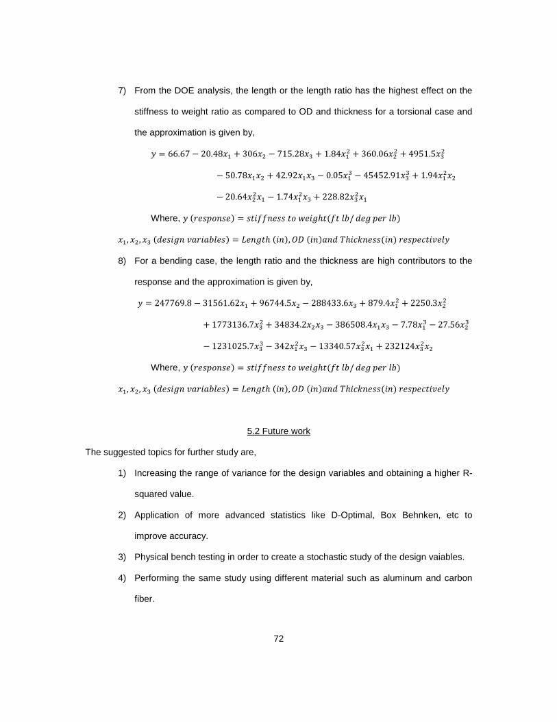
72

7) From the DOE analysis, the length or the length ratio has the highest effect on the

stiffness to weight ratio as compared to OD and thickness for a torsional case and

the approximation is given by,

4 � 66.67 ? 20.48�� @ 306�� ? 715.28�� @ 1.84�� @ 360.06�� @ 4951.5��

? 50.78�� @ 42.92�� ? 0.05�� ? 45452.91�� @ 1.94��? 20.64�� ? 1.74�� @ 228.82��


8) For a bending case, the length ratio and the thickness are high contributors to the

response and the approximation is given by,

4 � 247769.8 ? 31561.62�� @ 96744.5�� ? 288433.6�� @ 879.4�� @ 2250.3��

@ 1773136.7�� @ 34834.2�� ? 386508.4�� ? 7.78�� ? 27.56��

? 1231025.7�� ? 342�� ? 13340.57�� @ 232124��


5.2 Future work

The suggested topics for further study are,

1) Increasing the range of variance for the design variables and obtaining a higher R-

squared value.

2) Application of more advanced statistics like D-Optimal, Box Behnken, etc to

improve accuracy.

3) Physical bench testing in order to create a stochastic study of the design vaiables.

4) Performing the same study using different material such as aluminum and carbon

fiber.

73

APPENDIX A

SAMPLE ANSYS CODES FOR TORSIONAL TESTING

OF RECTANGULAR STRUCTURE

74

KEYW,PR_STRUC,1 !Selecting structural menu (preferences) KEYW,PR_THERM,0 KEYW,PR_FLUID,0 KEYW,PR_ELMAG,0 KEYW,MAGNOD,0 KEYW,MAGEDG,0 KEYW,MAGHFE,0 KEYW,MAGELC,0 KEYW,PR_MULTI,0 KEYW,PR_CFD,0 /prep7 ET,1,BEAM188 !Beam Type MPTEMP,,,,,,,, !Material Property MPTEMP,1,0 MPDATA,EX,1,,2.97e7 !Modulus of Elasticity MPDATA,PRXY,1,,.29 !Poisson's Ratio (.29) SECTYPE, 1, BEAM, CTUBE, , 0 !Beam Section Type SECOFFSET, CENT SECDATA,.472,.5,10,0,0,0,0,0,0,0 k,1,0,0,0,,,, !Creating keypoints k,2,5,0,0,,,, k,3,5,5,0,,,, k,4,0,5,0,,,, l,1,2 !Creating line elements l,2,3 l,3,4 l,4,1 FLST,5,12,4,ORDE,2 !Meshing the lines with the circular cross section FITEM,5,1 FITEM,5,-12 CM,_Y,LINE LSEL, , , ,P51X CM,_Y1,LINE CMSEL,,_Y LESIZE,_Y1,.2, , , , , , ,1 !Mesh every .20 inches FLST,2,12,4,ORDE,2 FITEM,2,1

75

FITEM,2,-12 LMESH,P51X /eshape,1 /GO !Applying constraints DK,4, ,0, ,0,UX,UY,UZ, , , , FLST,2,1,3,ORDE,1 FITEM,2,4 !* /GO DK,1, ,0, ,0,UX,UZ, , , , , FLST,2,1,3,ORDE,1 FITEM,2,2 !* /GO DK,3, ,0, ,0,UZ, , , , , , FLST,2,1,3,ORDE,1 FITEM,2,3 !* /GO !Applying loads FK,2,FZ,100 FINISH /SOL ! /STATUS,SOLU SOLVE FINISH /post1 !Postprocessing PRRSOL !List all Nodal Reactions PLESOL, S,EQV, 0,1.0 !Von Mises Stress Plot

76

REFERENCES

1. Costin, M., Phipps, D., 1961, Racing and Sports Car Chassis Design, B.T.Batsford Ltd, London, pp. 1-16

2. Wan, M., 1998, “ Different Types of Chassis,” AutoZine Technical School, http://www.autozine.org/technical_school/chassis/tech_chassis.htm

3. Chen, W., Lui, E.M., 2005, Handbook of Structural Engineering-2nd edition, CRC Press.

4. Gartner, M., 1999, “Chassis Design Tips”, http://www.gmecca.com/byorc/dtipschassis.html

5. Riley, W.B., George, A.R., 2002, “Design, Analysis and Testing of a Formula SAE Car Chassis,” SAE International, Warrendale, PA.

6. Heisler, H., 2002, Advanced Vehicle Technology, Butterworth-Heinemann, Woburn, MA. pp. 1

7. Perry, D.J., Azar, J.J., 1982, Aircraft Structure, McGraw Hill College. pp. 98, 197

8. Milliken, W.F., Milliken, D.L., 1997, Race Car Vehicle Dynamics, Society of Automotive Engineers.

9. Miller, C.M, 1997, Tubing Rigidity, http://desperadocycles.com/Lowdown_On_Tubing.html

10. Logan, D.L., 1992, A First Course in the Finite Element Method-2nd edition, PWS Kent, Boston.

11. Norton, R.L., 2010, Machine Design- 4th edition, Prentice Hall.

12. Potts, D.M., Zdravkovic, L., 1999, Finite Element Analysis in Geotechnical Engineering: Theory, Thomas Telford, London. pp. 74-75

77

13. Young, W.C., Budynas, R.G., 2002, Roark’s Formulas for Stress and Strain, McGraw Hill, pp. 534, 735

14. Altair Engineering Inc., Introduction to Hyperstudy. pp. 39-84

15. Walepole, R.E., Myers, S.L., Ye, K., 2007, Probability and Statistics for Engineers and Scientists, Pearson Education, Inc., pp. 421-433

78

BIOGRAPHICAL INFORMATION

Vikram Nair, son of E. Raghavan and Pratibha Raghavan, was born on February 14,

1988, in Chennai, India. He earned his Bachelor of Science in Mechanical Engineering in May,

2009 from University of Mumbai, India.

He started his graduate studies at University of Texas at Arlington in January, 2010 and

earned his Master of Science in Mechanical Engineering in May, 2012. During this time, Vikram

was part of the Formula SAE racing team at UTA where he worked on frame design and also

the design of an accumulator system for the Hybrid vehicle. He also worked as a Growth R&D

Co-op at Medtronic Powered Surgical Solutions which involved new product design and testing

of surgical equipment. His research involved the estimation of important factors which effect

torsional and flexural rigidity of a space frame under the supervision of Dr. Robert Woods.

Documents

DETERMINATION OF FACTORS TO IMPROVE EFFECTIVENESS OF