Policy ReseaRch WoRking PaPeR 4830

Determinants of Economic Growth

A Bayesian Panel Data Approach

Enrique Moral-Benito

The World BankDevelopment Research GroupMacroeconomics and Growth TeamFebruary 2009

WPS4830

Produced by the Research Support Team

Abstract

The Policy Research Working Paper Series disseminates the findings of work in progress to encourage the exchange of ideas about development issues. An objective of the series is to get the findings out quickly, even if the presentations are less than fully polished. The papers carry the names of the authors and should be cited accordingly. The findings, interpretations, and conclusions expressed in this paper are entirely those of the authors. They do not necessarily represent the views of the International Bank for Reconstruction and Development/World Bank and its affiliated organizations, or those of the Executive Directors of the World Bank or the governments they represent.

Policy ReseaRch WoRking PaPeR 4830

Model uncertainty hampers consensus on the key determinants of economic growth. Some recent cross-country, cross-sectional analyses have employed Bayesian Model Averaging to address the issue of model uncertainty. This paper extends that approach to panel data models with country-specific fixed effects. The empirical results show that the most robust growth determinants are the price of investment goods, distance

This paper—a product of the Growth and the Macroeconomics Team, Development Research Group—is part of a larger effort in the department to assess the determinants of economic growth. Policy Research Working Papers are also posted on the Web at http://econ.worldbank.org. The author may be contacted at emoral@cemfi.es.

to major world cities, and political rights. This suggests that growth-promoting policy strategies should aim to reduce taxes and distortions that raise the prices of investment goods; improve access to international markets; and promote democracy-enhancing institutional reforms. Moreover, the empirical results are robust to different prior assumptions on expected model size.

Determinants of Economic Growth:A Bayesian Panel Data Approach�

Enrique Moral-Benitoy

CEMFI

�This paper was completed during my stay at the World Bank�s research department. I wouldlike to thank Luis Servén and Manuel Arellano for his overall guidance and insightful comments.I also thank Roberto León, Eduardo Ley and Ignacio Sueiro for their help and advice. All errorsare my own.

yE-mail address: emoral@cem�.es, or enrique.moral@gmail.com

1

1 Introduction

Over the last two decades, hundreds of empirical studies have attempted to iden-tify the determinants of growth. This is not to say that growth theories are ofno use for that purpose. Rather, the problem is that growth theories are, usinga term due to Brock and Durlauf (2001), open-ended. This means that di¤er-ent growth theories are typically compatible with one another. For example, atheoretical view holding that trade openness matters for economic growth is notlogically inconsistent with another theoretical view that emphasizes the role ofgeography in growth. This diversity of theoretical views makes it hard to identifythe most e¤ective growth-promoting policies. The aim of this paper is to shedsome light on this issue.From an empirical point of view, the problem this literature faces is known

as model uncertainty, which emerges because theory does not provide enoughguidance to select the proper empirical model. In the search for a satisfactorystatistical model of growth, the main area of e¤ort has been the selection ofappropiate variables to include in linear growth regressions. The cross-countryregression literature concerned with this task is enormous: a huge number ofpapers have claimed to have found one or more variables correlated with thegrowth rate, resulting in a total of more than 140 variables proposed as growthdeterminants.A more speci�c issue was raised by Levine and Renelt (1992). From an

extreme-bounds analysis, they concluded that very few variables were robustlycorrelated with growth. In contrast, Sala-i-Martin (1997) constructed weightedaverages of OLS coe¢ cients and found that some were fairly stable across speci-�cations.Many researchers consider that the most promising approach to accounting

for model uncertainty is to employ model averaging techniques to construct para-meter estimates that formally address the dependence of model-speci�c estimateson a given model. In this context, Sala-i-Martin, Doppelhofer and Miller (2004)-henceforth SDM- employ their Bayesian Averaging of Classical Estimates (here-after, BACE) to determine which growth regressors should be included in linearcross-country growth regressions, making an attempt to con�rm in a Bayesian-inspired framework the results obtained by Sala-i-Martin (1997). In a pure Bayesianspirit, Fernandez, Ley and Steel (2001a) -henceforth FLS- apply the BayesianModel Averaging approach with di¤erent priors but the same objective. More-over, both methodologies allow constructing a ranking of variables ordered bytheir robustness as growth determinants. In spite of the focus on robustness ofthis approach, Ley and Steel (2007) show that the results are fairly sensitive tothe use of di¤erent prior assumptions. Moreover, Ciccone and Jarocinski (2005)employ exactly the same methodologies and conclude that the list of growth deter-minants emerging from these approaches is sensitive to arguably small variationsin the international income data used in the estimations.The main objective of this paper is to extend the Bayesian Model Averaging

2

(BMA) methodology to a panel data framework. The use of panel data in empiri-cal growth regressions has many advantages with respect to typical cross-countryregressions. First of all, the prospects for reliable generalizations in cross-countrygrowth regressions are often constrained by the limited number of countries avail-able, therefore, the use of within-country variation to multiply the number ofobservations is a natural response to this constraint. On the other hand, the useof panel data methods allows to solve the inconsistency of empirical estimateswhich typically arises with omitted country speci�c e¤ects which, if not uncorre-lated with other regressors, lead to a misspeci�cation of the underlying dynamicstructure, or with endogenous variables which may be incorrectly treated as ex-ogenous. Since the seminal work of Islam (1995), a lot of studies such as Caselli,Esquivel and Lefort (1996) have employed panel data models with country speci�ce¤ects in empirical growth regressions.In our case, to simultaneously address both omitted variable bias and issues

of endogeneity, we employ a Maximum Likelihood estimator which is able to usethe within variation across time and also the between variation across countries.Against this background, the paper presents a novel approach, Bayesian Av-

eraging of Maximum Likelihood Estimates (BAMLE), which is easy to interpretand easy to apply since it only requires the elicitation of one hyper-parameter,the expected model size, m. Moreover, the impact of di¤erent prior assumptionsabout m is minimal with the prior structure employed. Our methodology is sim-ilar to the BACE approach by SDM, but given the use of a maximum likelihoodestimator, BAMLE is more �exible and it can be applied to a broader range ofsituations. In fact, under the assumption of spherical disturbances, BACE can beconsidered a particular case of BAMLE.On the other hand, empirical results indicate that the sensivity of the list of

robust growth determinants emerging from our approach to the choice of alter-native sources of international income data is considerably smaller than found inthe previous literature. The reason is that the number of potential regressors weinclude in our dataset is much smaller than the number considered in previousstudies. Therefore, we conclude that the sensitivity of the results to variations inthe source of international income data found by Ciccone and Jarocinski (2005) isalso present when we consider country speci�c e¤ects. However, given our results,we can also conclude that the fewer the regressors the smaller the sensitivity. Forthe purposes of robustness, this suggests that the set of candidate variables shouldavoid inclusion of multiple proxies for the same theoretical e¤ect.The remainder of the paper is organized as follows. Section 2 describes the

BMA methodology and extends to the panel data case the prior structures pro-posed by SDM and FLS. Section 3 constructs the likelihood function, describesthe use of the BIC approximation in the BMA context, and introduces the priorassumptions employed for implementation of the BAMLE approach. In Section4 we brie�y describe the data set. The empirical results employing two di¤erentsources for international income data (World Development Indicators 2005 -WDI2005- and Penn World Table 6.2 -PWT 6.2-) are presented in Section 5. The �nal

3

section concludes.

2 Bayesian Model Averaging

A generic representation of the canonical growth regression is:

= �X + "; (1)

where is the vector of growth rates, and X represents a set of growth determi-nants, including those originally suggested by Solow as well as others 1. Thereexist potentially very many empirical growth models, each given by a di¤erentcombination of explanatory variables, and each with some probability of beingthe �true�model. This is the starting point of the Bayesian Model Averagingmethod.However, there is one variable for which theory o¤ers strong guidance, and

is therefore exempt from the problem of model uncertainty: initial GDP, whichshould always be included in growth regressions (see Durlauf, Johnson and Temple2005). As a result, in the remainder of the paper initial GDP will be includedwith probability 1 in all models under consideration.Using the Bayesian jargon, a model is formally de�ned by a likelihood function

and a prior density. Suppose we have K possible explanatory variables. We willhave 2K possible combinations of regressors, that is to say, 2K di¤erent models- indexed by Mj for j = 1; :::; 2K- which all seek to explain y -the data-. Mj

depends upon parameters �j. In cases where many models are being entertained,it is important to be explicit about which model is under consideration. Hence,the posterior for the parameters calculated using Mj is written as:

g��jjy;Mj

�=f�yj�j;Mj

�g��jjMj

�f (yjMj)

; (2)

and the notation makes clear that we now have a posterior, a likelihood, and aprior for each model. The logic of Bayesian inference suggests that we use Bayes�rule to derive a probability statement about what we do not know (i.e. whethera model is correct or not) conditional on what we do know (i.e. the data). Thismeans the posterior model probability can be used to assess the degree of supportfor Mj. Given the prior model probability P (Mj) we can calculate the posteriormodel probability using Bayes Rule as:

P (Mjjy) =f (yjMj)P (Mj)

f (y): (3)

Since P (Mj) does not involve the data, it measures how likely we believeMj to be the correct model before seeing the data. f (yjMj) is often called the

1The inclusion of additional control variables to the regression suggested by the Solow (oraugmented Solow) model can be understood as allowing for predictable and additional hetero-geneity in the steady state

4

marginal (or integrated) likelihood, and is calculated using (2) and a few simplemanipulations. In particular, if we integrate both sides of (2) with respect to�j, use the fact that

Rg��jjy;Mj

�d�j = 1 (since probability density functions

integrate to one), and rearrange, we obtain:

f (yjMj) =

Zf�yj�j;Mj

�g��jjMj

�d�j: (4)

The quantity f (yjMj) given by equation (4) is the marginal probability of thedata, because it is obtained by integrating the joint density of (y; �j) given y over�j. The ratio of integrated likelihoods of two di¤erent models is the Bayes Factorand it is closely related to the likelihood ratio statistic, in which the parameters�j are eliminated by maximization rather than by integration.Moreover, considering � a function of �j for each j = 1; :::; 2K , (i.e. for each

model j,� is de�ned as the vector �j augmented with zeros for those regressors notincluded in model j) we can also calculate the posterior density of the parametersfor all the models under consideration:

g (�jy) =X2K

j=1P (Mjjy) g (�jy;Mj) (5)

If one is interested in point estimates of the parameters, one common procedureis to take expectations across (5):

E (�jy) =X2K

j=1P (Mjjy)E (�jy;Mj) : (6)

Following Leamer (1978), we calculate the posterior variance as:

V (�jy) =X2K

j=1P (Mjjy)V (�jy;Mj) + (7)

+X2K

j=1P (Mjjy) (E (�jy;Mj)� E (�jy))2 :

Inspection of (7) shows that the posterior variance incorporates both the es-timated variances of the individual models as well as the variance in estimates ofthe ��s across di¤erent models.In words, the logic of Bayesian inference implies that one should obtain results

for every model under consideration and average them using appropiate weights.However, implementing Bayesian Model Averaging can be di¢ cult since the num-ber of models under consideration -2K-, is often huge. This has led to variousalgorithms which do not require dealing with every possible model. In particu-lar we will employ the so called Markov Chain Monte Carlo Model Composition(MC3) algorithm (see the Computational Appendix for more details).Given the above, we are now ready to introduce our measure of robustness.

We estimate the posterior probability that a particular variable h is included inthe regression, and we interpret it as the probability that the variable belongs inthe true growth model. In other words, variables with high posterior probabilities

5

of being included are considered as robust determinants of economic growth. Thisis called the posterior inclusion probability for variable h, and it is calculated asthe sum of the posterior model probabilities for all of the models including thatvariable:

posterior inclusion probability = P (�h 6= 0jy) =X

�h 6=0P (Mjjy) : (8)

2.1 BACE-SDM Approach in a Panel Data Context

For a given group of regressors, that is, for a given model Mj, the estimatedeconometric model consists of the following equation and assumptions:

yit � yit�� = �yit�� + x0jit�

j + �i + �t + vit (t = 1; :::; T ) (i = 1; :::; N) (9)

yit = �yit�� + x0jit�

j + �i + �t + vit (� = �+ 1)

E�vijyi; xji ; �i

�= 0; (A1)

where vi = (vi1; :::; viT )0, xji =

�xji1; :::; x

jiT

�0and yi = (yi1; :::; yiT )

0. We observe yit(the log of per capita GDP for country i in period t) and the kjx1 vector of ex-planatory variables xjit included in modelMj, but not �i, which is an unobservabletime-invariant regressor. Additionally, we assume:

V ar�vijyi; xji ; �i

�= �2IT : (A2)

Under assumptions (A1) and (A2), the within-group estimator (henceforth,WG) is the optimal estimator of � and �j for a given model.Note that in addition to the individual speci�c �xed e¤ect �i, we have also

included the term �t in (9). That is to say, we are including time dummies inthe model in order to capture unobserved common factors across countries andtherefore we are not ruling out cross-sectional dependence. In the practice, this isdone by simply working with cross-sectionally de-meaned data. In the remainingof the exposition, we assume that all the variables are in deviations from theircross-sectional mean.Following Sala-i-Martin et al. (2004) we have implemented the denominated

BACE approach in this context. The idea of BACE is to assume di¤use priors(as an indication of our ignorance) and make use of the result that, in the lin-ear regression model, for a given model Mj, standard di¤use priors and Bayesianregression yield posterior distributions identical to the classical sampling distrib-ution of OLS.With the assumptions stated above we can rewrite (6) as:

E (�jy) =P2K

j=1 P (Mjjy)b�j; (10)

where b�j is the WG2 estimate for � with the regressor set that de�nes model j.2Although assumption (A1) does not hold by de�nition in this context, we should remark

that this is the easiest way of applying the methodology to panel data estimates and we canconsider it as the starting point of our research.

6

Moreover, as the posterior odds�behavior is problematic with di¤use priors3, SDMpropose to use instead the Schwarz aymptotic approximation to the Bayes factor;therefore:

P (Mjjy) =P (Mj) (NT )

�kj=2 SSE�(NT )=2jP2K

i=1 P (Mi) (NT )�ki=2 SSE

�(NT )=2i

; (11)

where NT is the number of observations, K is the total number of regressors, kj

is the number of regressors included in model j and SSEj is the sum of squaredresiduals of the j-model�s regression. Regarding the prior model size (W ), theBACE approach assumes that each variable is independently included in a model:

W � Bin (K; �) (12)

E (W ) = K� ) � =m

K:

Note that with this prior structure, the researcher only needs to �x the priorexpected model size m which implies di¤erent prior inclusion probabilities for agiven regressor (�).

2.2 BMA-FLS Approach in a Panel Data Context

One question that arises when we think in terms of Bayesian econometrics ishow sensitive are the results to the choice of priors by the researcher? In thissection, instead of the BACE approach based on di¤usse priors, we implementthe full Bayesian approach with the benchmark priors proposed by Fernández,Ley and Steel (2001b). These priors can be easily applied to the panel data case(�xed-e¤ects model) if we rewrite the Mj model in the previous section as:

yit = �yit��+x0jit�

j+�1D1+ :::+�NDN+�t+vit (t = 1; :::; T ) (i = 1; :::; N); (13)

where the coe¢ cients (�1:::�N) are the individual unobservable e¤ects for eachcountry, (D1:::DN) are N dummy regressors and again, all variables will be indeviations from their cross-sectional means given the presence of the time dummy�t. Assumptions (A1) and (A2) also hold here, and the error term is supposed tofollow a normal distribution. Fernández et al. (2001b) propose a natural conjugateprior distribution which allows employing the exact Bayes factor instead of usingasymptotic approximations. For the variance parameter, which is common for allthe models under consideration, the prior is improper and non-informative:

p (�) / ��1: (14)

3If we use noninformative priors for parameters not common to all the considered models, theposterior odds ratio will always lend overwhelming support for the model with fewer parameters,regardless of the data.

7

The g-prior (Zellner (1986)) for the slope parameters is a normal density withzero mean and covariance matrix equal to:

�2�g0Z

0jZj��1

; (15)

where Zj = (y�1; xj; D1; :::; DN) and:

g0 = min

�1

NT;

1

(kj +N)2

�:

With this prior, both the posterior for each model and the Bayes factor havea closed form. Concretely, the Bayes factor (the ratio of integrated likelihoods)for model Mj versus model Mi is given by:

Bji =

�goj

1 + goj

� kj+1

2�goi + 1

goi

� ki+1

2

1

goi+1SSEi +

goigoi+1

(y0y)1

goj+1SSEj +

gojgoj+1

(y0y)

!NT2

: (16)

Once we have speci�ed the distribution of the observables given the parametersand the prior for these parameters, we only need to de�ne the prior probabilitiesfor each of the models. In particular, FLS assume that every model has the samea priori probability of being the true model:

P (Mj) = 2�K : (17)

The prior in (17) is the Binomial prior of SDM but employingm = K=2 insteadof m = 74.

2.3 On the E¤ect of Prior Assumptions

We have presented and described two di¤erent prior structures employed in theBMA context. Both approaches give very similar results, and this is often mis-interpreted as a symptom of robustness with respect to prior assumptions. Leyand Steel (2007) show that this similarity arises mostly by accident. The reasonis that the di¤erent choices of the prior inclusion probability of each variable (�) �treated as �xed in both approaches �compensates the di¤erent penalties to largermodels implied by the di¤use priors of SDM and the informative g-priors of FLS.The e¤ect of weakly-held prior views (as those that apply in the growth re-

gression context) should be minimal. In search of this minimal e¤ect, Ley andSteel (2007) propose a model prior speci�cation and model size (W ) given by thefollowing assumptions:

W � Bin (K; �) (18)

4This represents another di¤erence with respect to the priors of the BACE-SDM approach inthe previous subsection. Note that Sala-i-Martin et. al. (2004) propose m = 7 as a reasonableprior mean model size in the cross-country context. Here, we propose m = 5 for the panel datacase.

8

� � Be (a; b) ; (19)

where a; b > 0 are hyper-parameters to be �xed by the researcher. The di¤erencewith respect to SDM and FLS is to make � random rather than �xed. Model sizeW will then satisfy:

E (W ) =a

a+ bK: (20)

The prior model size distribution generated in this way is the so-called Binomial-Beta distribution. Ley and Steel (2007) propose to �x a = 1 and b = (K �m)=mthrough equation (20), so we only need to specify m, the prior mean model size,as in the BACE-SDM and BMA-FLS approaches.As shown by Ley and Steel (2007), this prior speci�cation with � random

rather than �xed implies a substantial increase in prior uncertainty about modelsize, and makes the choice of m much less critical. Moreover, as we shall see later,with random � the e¤ects of prior assumptions are much less severe.

3 Bayesian Averaging of Maximum LikelihoodEstimates (BAMLE)

The BAMLE approach is based on averaging maximum likelihood estimates in aBayesian spirit, i.e., we rewrite equation (6) as follows:

E (�jy) =P2K

j=1 P (Mjjy)b�jML: (21)

where b�jML is the maximum likelihood estimate for � in model j.The argument behind equation (21) is twofold: (i) assuming di¤use priors on

the parameter space of a given model, the posterior mode coincides with the MLE.(ii) in large samples, for any given prior, the posterior mode is very close to theMLE.Therefore, if we face a situation with either no prior information and any

sample size or any informative prior and a large sample, we can avoid Bayesiancalculations and controversies by using a maximum likelihood estimator. Thismakes BAMLE easy to interpret, easy to apply and more �exible than BACE.

3.1 The Likelihood Function

The panel data methods employed in the aforementioned approaches only permituse of the within variation in the data, and therefore cannot exploit the informa-tion contained in regressors without time variation. This situation implies thatwe are not considering all the potential determinants of economic growth. For in-stance, some theories argue that geographic factors without time variation matterfor growth. Moreover, as it is well-known, since assumption (A1) does not holdin dynamic panels, the within estimator of � is biased when T is small, as will beour case. Given the importance of this parameter -the convergence parameter- in

9

the growth context, it is desirable to get an unbiased estimator of �. Given theBayesian spirit of the approach, we propose here to use a maximum likelihoodestimator - for a given model - which permits addressing the two drawbacks justdescribed.For a given model Mj we can write:

yit = �yit�� + x0jit�

j + zji j + �i + �t + vit

Moreover, we can go further and assume5:

vitjyit�1:::yi0; xji ; zji ; �i � N

�0; �2v

�(A3)

�ijyi0; xji ; z

ji � N

�'yi0 + �

jxji ; �2�

�(A4)

Under assumptions (A3) and (A4) we can write the likelihood as6:

log f�yijyi0; xji ; z

ji

�/ �T � 1

2log �2v � (22)

� 1

2�2v

�y�i � �y�i(�1) � x

�ji �

j�0 �y�i � �y�i(�1) � x

�ji �

j��

�12log!2 � 1

2!2�yi � �yi(�1) � jz

ji � �jx

ji � 'yi0

�2;

where �j = �j + �j, ' and !2 are the linear projection coe¢ cients of ui on xji

and yi0, and y�i , y�i(�1) and x

�ji denote orthogonal deviations of yi, yi(�1) and x

ji

respectively.Thus, the Gaussian log-likelihood given yi0; x

ji and z

ji can be decomposed into

a within-group and a between-group component. This allows us to obtain anunbiased and consistent estimator for � (Alvarez and Arellano (2003)). Further-more, the between-group component together with the orthogonality assumptionbetween zji and �i allow for identi�cation of

j.We should emphasize that assumption (A4) implies that the regressors with

and without temporal variation are treated di¤erently. In the spirit of Hausmanand Taylor (1981) but in a simpler framework, it is important to note that whilethe x�s can be correlated with the unobservable �xed e¤ect, the z�s are inde-pendent. One interpretation is that, in addition to the traditional unobservedheterogeneity between countries given by the �i term, there also exists a secondtype of �xed but observable heterogeneity given by the zi variables. Moreover,both types of heterogeneity must be mutually uncorrelated. For instance, we maythink about observable geographic factors such as land area, which are indepen-dent from unobservables of each country as could be the ability of its population.With the BAMLE approach, we will be able to conclude which observable �xed

5Note that all data will be cross-sectional de-meaned given the inclusion of time dummies.6See Alvarez and Arellano (2003) for the demonstration in the pure autorregresive model.

We add here additional exogenous explanatory variables with and without temporal variation.

10

factors are more important in promoting economic growth. This conclusion couldalso be obtained by using standard random e¤ects estimation, but it is importantto remark that with our approach we do not need to assume independence be-tween the country speci�c e¤ect and time varying regressors, which seems to beimplausible in this context.

3.2 The BIC Approximation

Once we have speci�ed the likelihood function of the data, we need a few moreingredients for the implementation of the BAMLE methodology. An essential oneis the derivation of the integrated likelihood for a given model presented in equa-tion (4). Various analytic and numerical approximations have been proposed toaddress this problem. In particular, we will make use of the Bayesian InformationCriterion (BIC) approximation, which is both simple and accurate. The Schwarzcriterion gives a rough approximation to the logarithm of the Bayes factor, whichis easy to use and does not require evaluation of subjective prior distributions.We can approximate the Bayes factor between models Mi and Mj, Bij =

f(yjMi)f(yjMj)

such that (Raftery (1995)):

S= log f�yjb�i;Mi

�� log f

�yjb�j;Mj

��(ki � kj)

2log (NT ) ; (23)

where b�i is the MLE under Mi, ki is the dimension of b�i, and NT is the samplesize. As NT !1, this quantity, often called the Schwarz criterion, satis�es:

S � logBijlogBij

! 0 (24)

Minus twice the Schwarz criterion is often called the Bayesian informationcriterion (BIC):

BIC = �2S � �2 logBij: (25)

The relative error of exp(S) in approximating Bij is generally O(1). Thus evenfor very large samples, it does not produce the correct value. On the other hand,we must keep in mind that in our approach, testing two competing hypothesis isnot the �nal objective, and therefore we do not need the exact value of the Bayesfactor. Instead we only need a rough interpretation of Bij in a logarithmic scalesuch that7:

2 logBij Bij Interpretation by the MC3 algorithm> 0 > 1 Strong evidence against Mj

< 0 < 1 Not strong evidence against any model

7This is the interpretation we need for the implementation of our approach with the MC3

algorithm. See Computational Appendix for more details on the MC3 algorithm.

11

Equation (24) shows that in large samples the Schwarz criterion is equivalentto the logarithm of the Bayes factor and therefore it should provide a reasonableindication of this evidence.The value of BIC for model Mj denoted BICj, is the approximation to

�2logB0j given by (25), where B0j is the Bayes factor for model Mj againstM0 (which could be the null model with no independent variables). Moreover, wecan manipulate the previous equations in the following manner:

Bij =f (yjMi)

f (yjMj)=

f(yjMi)f(yjM0)

f(yjMj)

f(yjM0)

=Bi0Bj0

=B0jB0i

:

2 logBij = 2 [logB0j � logB0i] = �BICj +BICi:

In addition, we can rewrite equation (3) as:

P (Mjjy) =f (yjMj)P (Mj)P2K

i=1 f (yjMi)P (Mi)= (26)

=

f(yjMj)

f(yjMh)f (yjMh)P (Mj)P2K

i=1f(yjMi)f(yjMh)

f (yjMh)P (Mi)=

=Bjhf (yjMh)P (Mj)P2K

i=1Bihf (yjMh)P (Mi)=

=

1B0jP (Mj)P2K

i=11B0iP (Mi)

=Bj0P (Mj)P2K

i=1Bi0P (Mi);

where since B00 = 1, BIC0 = 0, then Bj0 = exp�12BICj

�.

Given the above, instead of integrating the marginal likelihood in (4), we willuse the following result:

f (yjMj) / exp�1

2BICj

�; (27)

and therefore:

P (Mjjy) =P (Mj) exp

�12BICj

�P2K

i=1 P (Mi) exp�12BICi

� : (28)

Furthermore, the posterior odds (posterior odds = prior odds xBayes Factor)becomes:

P (Mijy)P (Mjjy)

=P (Mi)

P (Mj)

exp�12BICi

�exp

�12BICj

� : (29)

3.3 The Choice of Priors

Bayesian inference may be controversial because it requires speci�cation of priordistributions which are subjectively chosen by the researcher. Moreover, Bayesian

12

calculations may be extremely hard and computationally demanding when esti-mating millions of non-regular models8.Given the use of a maximum likelihood estimator and the BIC approximation,

BAMLE avoids the need to specify a particular prior for the parameters of a givenmodel.As a result, for the implementation of BAMLE, the researcher only needs to

specify priors on the model space. In particular, in an attempt to limit the e¤ectsof weakly held prior views, we suggest to employ the Binomial-Beta prior structureproposed by Ley and Steel (2007), as described in the previous section.

4 Data

A huge number of variables have been proposed as growth determinants in thecross-country literature, including variables with and without time variation.However, data for many of the former is not available over the entire sampleperiod under consideration in this paper9. Since our main goal is to work with apanel data set, we limit our selection of time-varying variables to those for whichdata is available over the entire period 1960-2000.In the construction of our data set, we have considered two di¤erent criteria.

The �rst selection criterion derives from our aim of obtaining comparable resultswith the existing literature, and the second criterion comes from the fact that weneed to work with a balanced panel.With these restrictions, our data set includes a total of 35 variables (including

the dependent variable, the growth rate of per capita GDP) for 73 countries andfor the period 1960-2000. In order to avoid the problem of serial correlation inthe transitory component of the disturbance term, we have split our sample in�ve year periods. Therefore we have eight observations for each country, that isto say, we have a sample of 584 observations.Among the 19 regressors with temporal variation in our data set, there are

both stock and �ow variables. Following Caselli, Esquivel, and Lefort (1996),stock variables such as population and years of primary education are measuredin the �rst year of each �ve-year period. On the other hand, �ow variables suchas population growth and investment rate are measured as �ve-year averages.Finally, as we focus on 5-year periods, � = 5 in all our estimated models.

4.1 Determinants of Economic Growth

The augmented Solow model can be taken as the baseline empirical growth model.It comprises four determinants of economic growth, initial income, rates of human

8I refer here to non-regular models as those for which closed-form solutions are not availablewhen unsing informative priors.

9For instance, the fraction of GDP in mining and the fraction of Muslim population (bothconsidered in Fernández et. al. (2001a) and Sala-i-Martin et. al. (2004)) are only available forthe year 1960.

13

and physical capital accumulation, and population growth. We capture thesegrowth determinants through the ratio of real investment to GDP, the stock ofyears of education and demographic variables such as life expectancy, the ratioof labor force to total population and population growth. In addition to thosefour determinants, Durlauf, Johnson, and Temple�s (2005) survey of the empiricalgrowth literature identi�es 43 distinct growth theories and 145 proposed regressorsas proxies; each of these theories is found to be statistically signi�cant in at leastone study. Due to data availability, our set of growth determinants is a subsetof that identi�ed by Durlauf, Johnson and Temple (2005). We consider the threebroad variable categories below.

� Macroeconomic and external environment: A stable macroeconomic envi-ronment characterized by low and predictable in�ation, sustainable budgetde�cits, and limited departure of the real exchange rate from its equilibriumlevel sends important signals to the private sector about the commitmentand credibility of a country�s authorities to e¢ ciently manage their economyand increase the opportunity set of pro�table investments. In this paper,the impact of macroeconomic stability is captured by the government con-sumption relative to GDP. Since the seminal work of Barro (1991), manyauthors have considered this ratio (gc/GDP) as a measure of stability anddistortions in the economy. The argument is that government consumptionhas no direct e¤ect on private productivity but lowers saving and growththrough the distorting e¤ects from taxation or government-expenditure pro-grams. Moreover, following Easterly (1993) among others, we also considerthe investment price level (i.e., the PPP investment de�ator) as a proxyfor the level of distortions that exists in the economy. Finally, the traderegime/external environment is captured by the degree of trade openness,measured by imports plus exports as a share of GDP. Many authors suchas Levine and Renelt (1992) and Frankel and Romer (1999) have consideredthis ratio. However, since this measure is sometimes criticized because itonly captures the volume of trade and not the degree of openness as a proxyfor distortions in trade policies, we also consider an alternative indicator, theSW openness index constructed by Sachs and Warner (1995). The objectiveis to conclude which measure of openness is a better (in the sense of morerobust) proxy.

� Institutions and governance: The role of democracy and institutions in theprocess of economic growth has been the source of considerable researche¤ort. In this paper we examine the hypothesis that political freedom andinstitutional quality are signi�cant determinants of economic growth usingpolitical rights and civil liberties indices to measure the quality of institu-tions and capture the occurrence of free and fair elections and decentralizedpolitical power. Kormendi and Meguire (1985), Barro (1991), Barro and Lee(1994) and Sala-i-Martin (1997) among others considered these two indicesas proxies of the quality of institutions and governance.

14

� Geography and �xed factors: Following Sachs andWarner (1997) and Bloomand Warner (1998), there is an in�uential view arguing that di¤erences innatural endowments, such as climatic conditions can account for income dif-ferences accross countries. Very closely related, another view stresses marketaccess (remoteness) in explaining spatial variation in economic activity, asemphasized in the literature on new economic geography following Krug-man (1991). In order to examine the extent to which geography mattersfor growth, we use a variety of geographic indicators such as the percent-age of land area in the geographical tropics or the fraction of populationin geographical tropics. On the other hand, as proxies for remoteness weuse, among others, the minimal distance to New York, Rotterdam or Tokio,the fraction of land area near navigable water and a dummy for landlockedcountries. Finally, other �xed but not geographic factors such as the activeparticipation in con�icts during the sample period10 (war dummy) or thetiming of independence, may have an e¤ect on economic growth as pointedout by Barro and Lee (1994) and Gallup et. al. (2001) respectively.

A list of variables with their corresponding description and sources can befound in the Data Appendix, as well as the list of countries included in the sample.

5 Results

Table 1 reports the posterior inclusion probability of the 19 regressors with timevariation included in our data set after applying BACE-SDM and BMA-FLS pro-cedures. The table highlights the sensivity of the results to the di¤erent priorassumptions. Concretely, comparison of columns 1 and 3, and 2 and 4, showsthat with �xed � di¤erent assumptions about the prior mean model size, m = 5 orm = K=2, generate quite di¤erent posterior inclusion probabilities. More specif-ically, when we do not penalize larger models in any way �that is to say, whenwe employ m = K=2 instead of m = 5 in the BACE-SDM approach (columns3 and 1 respectively) �the posterior inclusion probabilities are higher. On theother hand, when we do penalize bigger models in both ways employing m = 5in the BMA-FLS approach (column 2), the posterior inclusion probabilities aresmaller. This also highlights the "fortuitous robustness" which emerges when wecompare the BMA-FLS and BACE-SDM�s results in columns 1 and 4, that isto say, di¤erent prior assumptions on model size have substantial e¤ects on theresults. Furthermore, analyzing columns 5 to 8 of Table 1, we can conclude thatthe e¤ects of prior assumptions on model size are much less important in the caseof random �. Moreover, the last row of the table indicates that expected modelsize should be close to 5 in the panel data framework.

10Given data availability and the requirement of a balanced panel, we follow Barro and Lee(1994) and use a dummy variable for countries that participated in at least one external war overthe period 1960-1990. Then, this variable is considered here as �xed over the sample period.

15

Table 2 shows the posterior inclusion probability, the posterior mean and theposterior standard error for the parameters corresponding to the 19 variables ofour data set with time variation when we apply the BACE-SDM and BMA-FLSapproaches in a panel data context. These results are based on the whole sample,that is, 73 countries for the period 1960-2000. The main conclusion from thetable is that, in addition to initial GDP, there are several covariates which appearrobustly related to economic growth. However, we defer our main conclusions toTable 4 below.In Tables 3 and 5, we follow the methodology employed by Ciccone and

Jarocinski (2005). Employing the same sample period for both sources of in-come data11, we can assess the sensitivity to changes in data source of the resultsin terms of posterior inclusion probability and posterior mean. The measuresshown are self-explanatory: the results are considerably less sensitive to di¤er-ences in income data source than found in the previous literature, at least for thecomparison between World Bank and Penn World Table income data12. In orderto further explore this issue, we redo the sensivity analysis using the BACE-SDMapproach without considering the panel structure of the data. By doing this, theonly di¤erence vis-a-vis Ciccone and Jarocinsky (2005) is the number of regressorsconsidered in the exercise. While they consider 67 potential explanatory variables,we consider 34. Looking at the results, presented in Table 6, we can see that thesensivity with K = 34 is much smaller than with K = 67. Therefore, we concludethat the number of potential explanatory variables under consideration is criticalfor the sensivity of the results to changes in the source of international incomedata used. Concretely, the fewer the regressors, the smaller the sensivity.Results when applying the BAMLE Approach with PWT 6.2 income data

for the whole period are summarized in Table 4. Addionally to initial GDP, afair number of regressors could be considered as robust determinants of economicgrowth accordingly to the Bayesian robustness check used in the approach. Themost conclusive evidence is for investment price, distance to major world cities andpolitical rights. All three regressors a¤ect growth with the expected sign: in par-ticular, as found by Easterly (1993), a low level of distorsions in the economy (i.e.lower investment price) would promote economic growth. A better geographic sit-uation, (i.e. a better access to international markets) is also an important growthenhancing factor as argued by Krugman (1991). Finally, in contrast to Barro(1991) but in line with Sala-i-Martin (1997), a higher level of democracy (i.e. alower value of the variable measuring restrictions on political rights) is found tobe positively related to higher growth rates. On the other hand, since their pos-terior inclusion probability is higher than their prior inclusion probability, manyother variables such as demographic indicators, a measure of trade openness, thedummy for landlocked countries, the investment share, the civil liberties indexand the government share can be considered as robust determinants of economicgrowth. Finally, there is one regressor, life expectancy, that poses a puzzle. In

11Note that WDI 2005 income data only covers the period 1975-2000.12See Ciccone and Jarocinski (2005) for more details on the cross-country context.

16

spite of having the highest posterior inclusion probability, we think it cannot beviewed as robust because its posterior standard error is bigger than its posteriormean. Despite the inclusion of country-speci�c e¤ects correlated with the time-varying variables, it is important to note that all these results must be interpretedwith some caution, since they assume that the x�s variables are strictly exogenouswith respect to the transitory component of the disturbance, which might not bea valid assumption in this context.It is worth mentioning that the posterior mean conditional on inclusion of the

lagged dependent variable (initial GDP) in Table 4 implies a rate of conditionalconvergence of � = 0:006. This suggest that after controlling for model uncertaintyand other potential inconsistencies afecting the lagged dependent variable (arisingfrom omitted variable and endogeneity biases), the estimated rate of convergenceis surprisingly similar to the standard cross-section �nding13.

6 Concluding Remarks

In spite of a huge amount of empirical research, the drivers of economic growthare not well understood. This paper attempts to provide insights on the growthpuzzle by searching for robust determinants of economic growth. We propose aBayesian Averaging of Maximum Likelihood Estimates (BAMLE) method in apanel data framework to determine which variables are signi�cantly related togrowth. Similarly to the BACE approach, our method is more appealing than astandard Bayesian Model Averaging since it does not require the speci�cation ofprior distributions for the parameters of every model under consideration, and itinvolves only one hyper-parameter, expected model sizem. Moreover, the BAMLEapproach is more �exible than BACE and it introduces two improvements withrespect to previous model-averaging and robustness-checking methods applied toempirical growth regressions: (i) it adressess the problem of inconsistent empiricalestimates by using a dynamic panel estimator, and (ii) it minimizes the impact ofprior assumptions about the only hyper-parameter in the approach. An additionalmethodological conclusion of the paper is that the list of growth determinantsemerging from a set of 34 potential explanatory variables is less sensitive to theuse of alternative sources of international income data than in the case of otherpapers which considered a larger number of potential regressors. Therefore, weconclude that the fewer the potential growth determinants considered, the smallerthe sensivity to changes in growth data.The empirical �ndings suggest that country speci�c e¤ects correlated with

other regressors play an important role since the list of robust growth determi-nants is not the same when we do not take into account their presence. Ourresults indicate that once model uncertainty and other potential inconsistenciesare accounted for, there exist economic, institutional, geographic and demographicfactors that robustly a¤ect growth. The most robust determinants are investment

13See for example Mankiw, Romer and Weil (1992, Table 4).

17

price, distance to major world cities and political rights. Other variables whichcan be considered as robust include demographic factors (population growth, ur-ban population and population), geographical dummies (such as the dummy forlandlocked countries), measures of openness and civil liberties, and macroeco-nomic indicators such as the investment share of GDP and the ratio of govern-ment consumption to GDP. On the other hand, our empirical estimate of the rateof convergence, after controlling for both model uncertainty and endogeneity, issurprisingly similar to that commonly found in cross-section studies.As a �nal remark, it is worth mentioning that the dynamic panel estimator

proposed in this paper addresses the endogeneity of regressors with time variationwith respect to the permanent component of the error term as well as the endo-geneity of the lagged dependent variable with respect to the transitory componentof the error term. However, many other regressors such as the labor force or theinvestment share should ideally be considered as predetermined instead of strictlyexogenous with respect to the transitory component of the error term, and thispoint remains unresolved in the BMA context. Hence, the estimates might changeunder less stringent exogeneity assumptions. This issue is left for future research.

18

A Appendix

A.1 Computational Appendix

For the implementation of the empirical approaches described in the paper, weneed to resort to the algorithms proposed in the literature because of the ex-tremely large number of calculations required for obtaining the posterior meanand variance described in equations (6) and (7). This is because the number ofpotential regressors determines the number of models under consideration, for ex-ample, in our case, with K = 35 potential regressors, the number of models underconsideration is 3:4x1010. These algorithms carry out Bayesian Model Averagingwithout evaluating every possible model.Concretely, for the BACE, BMA and BAMLE approaches we have made use

of the Markov Chain Monte Carlo Model Composition (MC3) algorithm pro-posed by Madigan and York (1995), which generates a stochastic process thatmoves through model space. The idea is to construct a Markov chain of mod-els fM(t); t = 1; 2; :::g with state space �. If we simulate this Markov chainfor t = 1; :::; N , then under certain regularity conditions, for any function h(Mi)de�ned on �, the average bH =

1

N

NXt=1

h (M (t))

converges with probability 1 to E (h (M)) as N ! 1. To compute (6) in thisfashion, we set h(Mi) = E(�jMi; y).To construct the Markov chain, we de�ne a neighborhood nbd(M) for each

M 2 � that consists of the model M itself and the set of models with eitherone variable more or one variable fewer than M . Then, a transition matrix q isde�ned by setting q(M ! M 0) = 0 8 M 0 =2 ndb(M) and q(M ! M 0) constantfor all M 0 2 ndb(M). If the chain is currently in state M , then we proceed bydrawing M 0 from q(M !M 0). It is the accepted with probability

min

�1;Pr (M 0jy)Pr (M jy)

�Otherwise, the chain stays in state M 14.After some experimentation with generated data, we verify the proper conver-

gence properties of our Gauss code which implements the described MC3 algo-rithm.

14Koop (2003) is a good reference for the reader interested in developing a deeper understand-ing of the MC3 algorithm.

19

A.2 Data AppendixTable A1: Variable De�nitions and Sources

Variable Source De�nitionDependent Variable PWT 6.2 Growth of GDP per capita over 5-year periods

(2000 US dollars at PPP)Initial GDP PWT 6.2 Logarithm of initial real GDP per capita

(2000 US dollars at PPP)Population Growth PWT 6.2 Average growth rate of populationPopulation PWT 6.2 Population in thousands of peopleTrade Openness PWT 6.2 Export plus imports as a share of GDPGovernment Share PWT 6.2 Government consumption as a share of GDPInvestment Price PWT 6.2 Average investment price levelLabor Force PWT 6.2 Ratio of workers to populationConsumption Share PWT 6.2 Consumption as a share of GDPInvestment Share PWT 6.2 Investment as a share of GDPUrban Population WDI 2005 Fraction of population living in urban areasPopulation Density WDI 2005 Population divided by land areaLife Expectancy WDI 2005 Life expectancy at birthPopulation under 15 Barro and Lee Fraction of population younger than 15 yearsPopulation over 65 Barro and Lee Fraction of population older than 65 yearsPrimary Education Barro and Lee Stock of years of primary educationSecondary Education Barro and Lee Stock of years of secondary educationPolitical Rights Freedom House Index of political rights from 1 (highest) to 7Civil Liberties Freedom House Index of civil liberties from 1 (highest) to 7Malaria Gallup et. al. Fraction of population in areas with malariaNavigable Water Gallup et. al. Fraction of land area near navigable waterLandlocked Country Gallup et. al. Dummy for landlocked countriesAir Distance Gallup et. al. Logarithm of minimal distance in km from

New York, Rotterdam, or TokioTropical Area Gallup et. al. Fraction of land area in geographical tropics

Notes:1. PWT 6.2 refers to Penn World Table 6.22. WDI 2005 refers to World Development Indicators 2005 from The World Bank

20

Table A1 - Continued

Variable Source De�nitionTropical Pop. Gallup et. al. Fraction of population in geographical tropicsLand Area Gallup et. al. Area in km2

Independence Gallup et. al. Timing of national independence measure: 0if before 1914; 1 if between 1914 and 1945; 2if between 1946 and 1989 and 3 if after 1989

Socialist Gallup et. al. Dummy for countries under socialist rule forconsiderable time during 1950 to 1995

Climate Gallup et. al. Fraction of land area with tropical climateWar Dummy Barro and Lee Dummy for countries that participated in ex-

ternal war between 1960 and 1990SW Openness Index Sachs, Warner Index of trade opennes from 1 (highest) to 0Europe Dummy for EU countriesSub-Saharan Africa Dummy for Sub-Saharan African countriesLatin America Dummy for Latin American countriesEast Asia Dummy for East Asian countries

21

Table A2: List of Countries

Algeria Indonesia PeruArgentina Iran PhilippinesAustralia Ireland PortugalAustria Israel RwandaBelgium Italy SenegalBenin Jamaica SingaporeBolivia Japan South AfricaBrazil Jordan SpainCameroon Kenya Sri LankaCanada Lesotho SwedenChile Malawi SwitzerlandChina Malaysia SyriaColombia Mali ThailandCosta Rica Mauritius TogoDenmark Mexico Trinidad & TobagoDominican Republic Mozambique TurkeyEcuador Nepal UgandaEl Salvador Netherlands United KingdomFinland New Zealand United StatesFrance Nicaragua UruguayGhana Niger VenezuelaGreece Norway ZambiaGuatemala Pakistan ZimbabweHonduras PanamaIndia Paraguay

22

References

[1] Alvarez, J. and M. Arellano (2003), "The Time Series and Cross-SectionAsymptotics of Dynamic Panel Data Estimators" Econometrica, Vol. 71, No.4. pp. 1121-1159.

[2] Barro, R. (1991), �Economic Growth in a Cross Section of Countries�Quar-terly Journal of Economics, 106, 2, 407-43

[3] Barro, R. and J.-W. Lee (1994), �Sources of Economic Growth�Carnegie-Rochester Conference Series on Public Policy, 40, 1-57.

[4] Bloom, D. and J. Sachs. (1998), �Geography, Demography and EconomicGrowth in Africa.�Brookings Papers on Economic Activity, 207� 73.

[5] Brock, W. and S. Durlauf (2001), "Growth Empirics and Reality" WorldBank Economic Review, 15, 2, pp. 229-272.

[6] Caselli, F., G. Esquivel and F. Lefort (1996), "Reopening the ConvergenceDebate: A New Look at Cross-Country Growth Empirics" Journal of Eco-nomic Growth, 1, pp. 363-389.

[7] Ciccone, A. and M. Jarocinski (2005), "Determinants of Economic Growth:Will Data Tell?" Unpublished manuscript.

[8] Durlauf, S., P. Johnson and J. Temple (2005), "Growth Econometrics" In P.Aghion and S.N. Durlauf, eds., Handbook of Economic Growth, Volume 1A,pp. 555-677, Amsterdam, North-Holland.

[9] Easterly, W. (1993), �How Much Do Distortions A¤ect Growth?�Journal ofMonetary Economics, 32, 2, 187-212.

[10] Fernandez, C., E. Ley and M. Steel (2001a), "Model Uncertainty in Cross-Country Growth Regressions" Journal of Applied Econometrics, 16, pp. 563-576.

[11] Fernandez, C., E. Ley and M. Steel (2001b), "Benchmark Priors for BayesianModel Averaging" Journal of Econometrics, 100, pp. 381-427.

[12] Frankel, J. and D. Romer (1999), �Does Trade Cause Growth?,�AmericanEconomic Review, 89, 3, 379-399.

[13] Gallup, J., A. Mellinger and J. Sachs (2001) �Geography Datasets�Centerfor International Development at Harvard University (CID)

[14] Hausman, J. andW. Taylor, (1981) "Panel Data and Unobservable IndividualE¤ects" Econometrica, Vol. 49, No. 6. pp. 1377-1398.

23

[15] Islam, N. (1995), "Growth Empirics: A Panel Data Approach" The QuarterlyJournal of Economics, Vol. 110(4), pp. 1127-70

[16] Kass, R. and A. Raftery (1995), "Bayes Factors" Journal of the AmericanStatistical Association, Vol. 90, No 430, pp. 773-795.

[17] Kormendi, R. and P. Meguire (1985), �Macroeconomic Determinants ofGrowth: Cross Country Evidence,�Journal of Monetary Economics, 16, 2,141-63.

[18] Krugman, P. (1991), �Increasing Returns and Economic Geography.�Journalof Political Economy, 99(3): 483� 99.

[19] León-González, R. and D. Montolio (2004), "Growth, Convergence and Pub-lic Investment: A BMA Approach" Applied Economics, 36, pp. 1925-36.

[20] Levine, R. and D. Renelt (1992), "A sensivity Analysis of Cross-CountryGrowth Regressions" American Economic Review, 82, pp. 942-963.

[21] Ley, E. and M. Steel (2007), "On the E¤ect of Prior Assumptions in BayesianModel Averaging with Applications to Growth Regression" Unpublishedmanuscript.

[22] Madigan, D. and J. York (1995), "Bayesian Graphical Models for DiscreteData" International Statistical Review, 63, pp. 215-232.

[23] Mankiw, N., D. Romer and D. Weil (1992), "A Contribution to the Empiricsof Economic Growth" Quarterly Journal of Economics, 107, pp. 407-437.

[24] Masanjala, W. and C. Papageorgiou (2005), "Rough and Lonely Road toProsperity: A reexamination of the sources of growth in Africa using BayesianModel Averaging" Unpublished manuscript.

[25] Raftery, A. (1995), "Bayesian Model Selection in Social Research" Sociologi-cal Methodology, Vol. 25, pp. 111-163.

[26] Raftery, A. (1996), "Approximate Bayes Factors and Accounting for ModelUncertainty in Generalized Linear Models" Biometrika, Vol. 83, No. 2.pp.251-266.

[27] Sachs, J. and Warner, A. (1995), �Economic Reform and the Process ofEconomic Integration�, Brookings Papers of Economic Activity, pp.1-95.

[28] Sachs, J. and Warner, A. (1997), �Natural Resource Abundance and Eco-nomic Growth�, CID at Harvard University.

[29] Sala-i-Martin, X. (1997), "I Just Ran Two Million Regressions" AmericanEconomic Review, Vol. 87, No. 2. pp. 178-183. Papers and Proceedings of theHundred and Fourth Annual Meeting of the American Economic Association.

24

[30] Sala-i-Martin, X., G. Doppelhofer and R. Miller (2004), "Determinants ofLong-Term Growth: A Bayesian Averaging of Classical Estimates (BACE)Approach" American Economic Review, Vol. 94, No. 4. pp. 813-835.

[31] Schwarz, G. (1978), "Estimating the Dimension of a Model" The Annals ofStatistics, Vol. 6, No. 2. pp. 461-464.

[32] Tsangarides, C. (2004), "A Bayesian Approach to Model Uncertainty" IMFWorking Paper WP/04/68.

[33] Tsangarides, C. (2005), "Growth Empirics Under Model Uncertainty: IsAfrica Di¤erent?" IMF Working Paper WP/05/18.

25

Tables

Table 1: Posterior Inclusion Probability of the Regressors

� Fixed � RandomVariable m = 5 m = K=2 m = 5 m = K=2

SDM FLS SDM FLS SDM FLS SDM FLS(1) (2) (3) (4) (5) (6) (7) (8)

Initial GDP 1.000 1.000 1.000 1.000 1.000 1.000 1.000 1.000Population 1.000 1.000 1.000 1.000 1.000 1.000 1.000 1.000Population under 15 0.950 0.961 0.937 0.953 0.953 0.965 0.949 0.963Investment Share 0.826 0.847 0.783 0.835 0.822 0.841 0.816 0.843Urban Population 0.651 0.392 0.781 0.596 0.608 0.358 0.638 0.387Consumption Share 0.305 0.100 0.682 0.229 0.303 0.088 0.351 0.099Trade Opennes 0.287 0.106 0.656 0.218 0.289 0.094 0.336 0.103Government Share 0.237 0.064 0.549 0.173 0.231 0.058 0.273 0.068Investment Price 0.222 0.088 0.376 0.176 0.206 0.083 0.229 0.092Population Density 0.031 0.013 0.061 0.024 0.029 0.011 0.033 0.013Labor Force 0.029 0.013 0.064 0.022 0.028 0.010 0.033 0.012Primary Education 0.026 0.010 0.061 0.023 0.026 0.009 0.030 0.010Civil Liberties 0.023 0.007 0.053 0.017 0.022 0.006 0.025 0.008Population Growth 0.018 0.005 0.050 0.013 0.019 0.005 0.022 0.005Life Expectancy 0.018 0.006 0.051 0.013 0.019 0.005 0.023 0.006Malaria 0.020 0.005 0.043 0.014 0.018 0.006 0.021 0.006Population over 65 0.017 0.005 0.044 0.013 0.018 0.004 0.021 0.006Secondary Education 0.017 0.005 0.046 0.012 0.017 0.005 0.020 0.005Political Rights 0.016 0.005 0.044 0.012 0.016 0.004 0.020 0.005Prior Mean Model Size 5 5 9 9 5 5 9 9Post. Mean Model Size 5.69 4.63 7.28 5.34 5.62 4.55 5.83 4.63Column heading SDM refers to the BACE-SDM Approach in a panel data context.Column heading FLS refers to BMA-FLS approach in a panel data context.

26

Table 2: SDM-FLS Approaches in a Panel Data Contextwith PWT 6.2 Income Data 1960-2000*

Posterior Inclusion Posterior PosteriorVariable Probability Mean Standard Error

SDM FLS SDM FLS SDM FLSInitial GDP 1.000 1.000 -0.271 -0.265 0.029 0.030Population 1.000 1.000 0.918 0.905 0.176 0.176Population under 15 0.953 0.965 -1.122 -1.183 0.287 0.279Investment Share 0.822 0.841 0.343 0.351 0.097 0.095Urban Population 0.608 0.358 -0.426 -0.433 0.147 0.147Consumption Share 0.303 0.088 -0.210 -0.202 0.068 0.091Trade Opennes 0.289 0.094 0.102 0.100 0.028 0.046Government Share 0.231 0.058 -0.336 -0.315 0.140 0.149Investment Price 0.206 0.083 -0.031 -0.033 0.014 0.014Population Density 0.029 0.011 0.042 0.063 0.054 0.057Labor Force 0.028 0.010 0.225 0.363 0.415 0.477Primary Education 0.026 0.009 -0.169 -0.194 0.179 0.186Civil Liberties 0.022 0.006 -0.044 -0.047 0.060 0.060Population Growth 0.019 0.005 -0.488 -0.317 1.156 1.091Life Expectancy 0.019 0.005 0.063 -0.011 0.241 0.250Malaria 0.018 0.006 0.010 0.013 0.024 0.026Population over 65 0.018 0.004 -0.220 -0.200 0.824 0.801Secondary Education 0.017 0.005 -0.051 -0.034 0.186 0.191Political Rights 0.016 0.004 -0.009 -0.004 0.048 0.049

*All results presented in this Table are based on prior assumptions m = 5 and �Random. The results with m = K=2 are not presented here for the sake of brevity, butthey were practically identical.

27

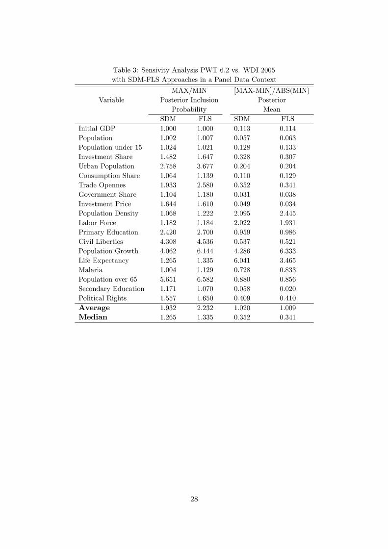
Table 3: Sensivity Analysis PWT 6.2 vs. WDI 2005with SDM-FLS Approaches in a Panel Data Context

MAX/MIN [MAX-MIN]/ABS(MIN)Variable Posterior Inclusion Posterior

Probability MeanSDM FLS SDM FLS

Initial GDP 1.000 1.000 0.113 0.114Population 1.002 1.007 0.057 0.063Population under 15 1.024 1.021 0.128 0.133Investment Share 1.482 1.647 0.328 0.307Urban Population 2.758 3.677 0.204 0.204Consumption Share 1.064 1.139 0.110 0.129Trade Opennes 1.933 2.580 0.352 0.341Government Share 1.104 1.180 0.031 0.038Investment Price 1.644 1.610 0.049 0.034Population Density 1.068 1.222 2.095 2.445Labor Force 1.182 1.184 2.022 1.931Primary Education 2.420 2.700 0.959 0.986Civil Liberties 4.308 4.536 0.537 0.521Population Growth 4.062 6.144 4.286 6.333Life Expectancy 1.265 1.335 6.041 3.465Malaria 1.004 1.129 0.728 0.833Population over 65 5.651 6.582 0.880 0.856Secondary Education 1.171 1.070 0.058 0.020Political Rights 1.557 1.650 0.409 0.410Average 1.932 2.232 1.020 1.009Median 1.265 1.335 0.352 0.341

28

Table 4: BAMLE Approach with PWT 6.2 Income Data 1960-2000*

Posterior Inclusion Posterior PosteriorVariable Probability Mean Standard Error

Initial GDP 1.000 -0.033 0.035Life Expectancy 1.000 0.145 0.287Investment Price 0.863 -0.049 0.015Air Distance 0.759 -0.962 0.381Political Rights 0.722 -0.053 0.013Population Growth 0.688 -1.082 1.081Urban Population 0.650 -0.475 0.163Population 0.639 0.602 0.201Trade Openness 0.467 0.056 0.020Landlocked Country 0.320 -0.346 0.359Investment Share 0.238 0.271 0.105Civil Liberties 0.176 0.048 0.017Government Share 0.161 -0.160 0.148Latin America 0.147 0.038 0.015Population Density 0.087 -0.014 0.081East Asia 0.073 -0.012 0.006Consumption Share 0.057 0.036 0.062Navigable Water 0.057 0.043 0.026Europe 0.052 -0.036 0.018Tropical Area 0.034 -0.252 0.201Sub-Saharan Africa 0.029 0.027 0.021Climate 0.028 -0.014 0.013Primary Education 0.028 0.024 0.022Tropical Pop. 0.025 -0.144 0.212Labor Force 0.023 0.028 0.394Population over 65 0.022 -0.012 0.018SW Openness Index 0.018 -0.033 0.069Land Area 0.017 0.021 0.056War Dummy 0.017 0.001 0.019Population under 15 0.017 0.010 0.012Secondary Education 0.017 -0.008 0.016Independence 0.016 -0.002 0.015Socialist 0.016 -0.009 0.013Malaria 0.013 0.001 0.012

*All results presented in this Table are based on prior assumptions m = 5 and �Random.

29

Table 5: Sensivity Analysis PWT 6.2 vs. WDI 2005 with BAMLE Approach

MAX/MIN [MAX-MIN]/ABS(MIN)Variable Posterior Inclusion Posterior

Probability MeanInitial GDP 1.000 0.140Life Expectancy 1.000 2.038Investment Price 1.182 0.063Air Distance 4.019 0.789Political Rights 1.149 0.061Population Growth 2.102 2.526Urban Population 3.645 0.486Population 1.215 0.221Trade Openness 3.268 3.667Landlocked Country 1.011 0.010Investment Share 4.289 0.368Civil Liberties 2.721 0.182Government Share 2.895 1.964Latin America 1.412 0.161Population Density 1.738 0.878East Asia 1.048 1.286Consumption Share 1.792 0.456Navigable Water 6.784 0.088Europe 2.308 0.667Tropical Area 1.154 0.878Sub-Saharan Africa 1.042 0.343Climate 2.079 0.346Primary Education 1.059 5.000Tropical Pop. 1.286 2.935Labor Force 1.571 0.448Population over 65 6.000 0.870SW Openness Index 4.333 0.424Land Area 1.882 0.518War Dummy 1.000 0.222Population under 15 1.643 0.250Secondary Education 1.067 1.000Independence 1.308 0.833Socialist 1.571 1.304Malaria 1.125 0.556Average 2.138 0.940Median 1.571 0.502

30

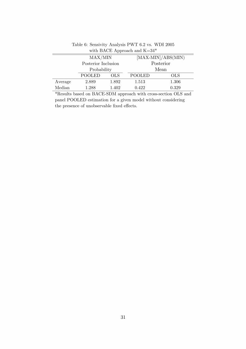
Table 6: Sensivity Analysis PWT 6.2 vs. WDI 2005with BACE Approach and K=34*

MAX/MIN [MAX-MIN]/ABS(MIN)Posterior Inclusion Posterior

Probability MeanPOOLED OLS POOLED OLS

Average 2.889 1.892 1.513 1.306Median 1.288 1.402 0.422 0.329*Results based on BACE-SDM approach with cross-section OLS andpanel POOLED estimation for a given model without consideringthe presence of unobservable �xed e¤ects.

31