Embed Size (px)
Citation preview
Department of Electrical and Computer Engineering 2009
Brigham Young University · Provo, Utah
Detection and Estimation Theory
Lecture Notes
For
ECEn 672
Prepared by
Wynn StirlingWinter Semester, 2009
Section 001
Copyright c© 2009, Wynn C. Stirling
0-2 ECEn 672
Contents
1 The Formalism of Statistical Decision Theory 1-1
1.1 Game Theory and Decision Theory . . . . . . . . . . . . . . . . . . . . . . . 1-1
1.2 The Mathematical Structure of Decision Theory . . . . . . . . . . . . . . . . 1-4
1.2.1 The Formalism of Statistical Decision Theory . . . . . . . . . . . . . 1-5
1.2.2 Special Cases . . . . . . . . . . . . . . . . . . . . . . . . . . . . . . . 1-9
2 The Multivariate Normal Distribution 2-1
2.1 The Univariate Normal Distribution . . . . . . . . . . . . . . . . . . . . . . . 2-1
2.2 Development of The Multivariate Distribution . . . . . . . . . . . . . . . . . 2-1
2.3 Transformation of Variables . . . . . . . . . . . . . . . . . . . . . . . . . . . 2-4
2.4 The Multivariate Normal Density . . . . . . . . . . . . . . . . . . . . . . . . 2-6
3 Introductory Estimation Theory Concepts 3-1
3.1 Notational Conventions . . . . . . . . . . . . . . . . . . . . . . . . . . . . . . 3-1
3.2 Populations and Statistics . . . . . . . . . . . . . . . . . . . . . . . . . . . . 3-2
3.2.1 Sufficient Statistics . . . . . . . . . . . . . . . . . . . . . . . . . . . . 3-3
3.2.2 Complete Sufficient Statistics . . . . . . . . . . . . . . . . . . . . . . 3-9
3.3 Exponential Families . . . . . . . . . . . . . . . . . . . . . . . . . . . . . . . 3-13
3.4 Minimum Variance Unbiased Estimators . . . . . . . . . . . . . . . . . . . . 3-17
4 Neyman-Pearson Theory 4-1
4.1 Hypothesis Testing . . . . . . . . . . . . . . . . . . . . . . . . . . . . . . . . 4-1
4.2 Simple Hypothesis versus Simple Alternative . . . . . . . . . . . . . . . . . . 4-2
4.3 The Neyman-Pearson Lemma . . . . . . . . . . . . . . . . . . . . . . . . . . 4-3
4.4 The Likelihood Ratio . . . . . . . . . . . . . . . . . . . . . . . . . . . . . . . 4-8
4.5 Receiver Operating Characteristic . . . . . . . . . . . . . . . . . . . . . . . . 4-11
4.6 Composite Binary Hypotheses . . . . . . . . . . . . . . . . . . . . . . . . . . 4-18
5 Bayes Decision Theory 5-1
5.1 The Bayes Principle . . . . . . . . . . . . . . . . . . . . . . . . . . . . . . . . 5-1

Winter 2009 0-3
5.2 Bayes Risk . . . . . . . . . . . . . . . . . . . . . . . . . . . . . . . . . . . . . 5-2
5.3 Bayes Tests of Simple Binary Hypotheses . . . . . . . . . . . . . . . . . . . . 5-4
5.4 Bayes Envelope Function . . . . . . . . . . . . . . . . . . . . . . . . . . . . . 5-10
5.5 Posterior Distributions . . . . . . . . . . . . . . . . . . . . . . . . . . . . . . 5-12
5.6 Randomized Decision Rules . . . . . . . . . . . . . . . . . . . . . . . . . . . 5-15
5.7 Minimax Rules . . . . . . . . . . . . . . . . . . . . . . . . . . . . . . . . . . 5-17
5.8 Summary of Binary Decision Problems . . . . . . . . . . . . . . . . . . . . . 5-18
5.9 Multiple Decision Problems . . . . . . . . . . . . . . . . . . . . . . . . . . . 5-18
5.10 An Important Class of M-Ary Problems . . . . . . . . . . . . . . . . . . . . 5-24
6 Maximum Likelihood Estimation 6-1
6.1 The Maximum Likelihood Principle . . . . . . . . . . . . . . . . . . . . . . . 6-1
6.2 Maximum Likelihood for Continuous Distributions . . . . . . . . . . . . . . . 6-5
6.3 Comments on Estimation Quality . . . . . . . . . . . . . . . . . . . . . . . . 6-8
6.4 The Cramer-Rao Bound . . . . . . . . . . . . . . . . . . . . . . . . . . . . . 6-9
6.5 Asymptotic Properties of Maximum Likelihood Estimators . . . . . . . . . . 6-15
6.6 The Multivariate Normal Case . . . . . . . . . . . . . . . . . . . . . . . . . . 6-20
6.7 Appendix: Matrix Derivatives . . . . . . . . . . . . . . . . . . . . . . . . . . 6-23
7 Conditioning 7-1
7.1 Conditional Densities . . . . . . . . . . . . . . . . . . . . . . . . . . . . . . . 7-1
7.2 σ-fields . . . . . . . . . . . . . . . . . . . . . . . . . . . . . . . . . . . . . . . 7-5
7.3 Conditioning on a σ-field . . . . . . . . . . . . . . . . . . . . . . . . . . . . . 7-10
7.4 Conditional Expectations and Least-Squares Estimation . . . . . . . . . . . 7-13
8 Bayes Estimation Theory 8-1
8.1 Bayes Risk . . . . . . . . . . . . . . . . . . . . . . . . . . . . . . . . . . . . . 8-3
8.2 MAP Estimates . . . . . . . . . . . . . . . . . . . . . . . . . . . . . . . . . . 8-6
8.3 Conjugate Prior Distributions . . . . . . . . . . . . . . . . . . . . . . . . . . 8-9
8.4 Improper Prior Distributions . . . . . . . . . . . . . . . . . . . . . . . . . . . 8-12
8.5 Sequential Bayes Estimation . . . . . . . . . . . . . . . . . . . . . . . . . . . 8-13
0-4 ECEn 672
9 Linear Estimation Theory 9-16
9.1 Introduction . . . . . . . . . . . . . . . . . . . . . . . . . . . . . . . . . . . . 9-16
9.2 Minimum Mean Square Estimation (MMSE) . . . . . . . . . . . . . . . . . . 9-18
9.3 Estimation Given a Single Random Variable . . . . . . . . . . . . . . . . . . 9-19
9.4 Estimation Given two Random Variables . . . . . . . . . . . . . . . . . . . . 9-20
9.5 Estimation Given N Random Variables . . . . . . . . . . . . . . . . . . . . . 9-21
9.6 Mean Square Estimation for Random Vectors . . . . . . . . . . . . . . . . . 9-23
9.7 Hilbert Space of Random Variables . . . . . . . . . . . . . . . . . . . . . . . 9-24
9.8 Geometric Interpretation of Mean Square Estimation . . . . . . . . . . . . . 9-27
9.9 Gram-Schmidt Procedure . . . . . . . . . . . . . . . . . . . . . . . . . . . . 9-29
9.10 Estimation Given the Innovations Process . . . . . . . . . . . . . . . . . . . 9-33
9.11 Innovations and Matrix Factorizations . . . . . . . . . . . . . . . . . . . . . 9-36
9.12 LDU Decomposition . . . . . . . . . . . . . . . . . . . . . . . . . . . . . . . 9-37
9.13 Cholesky Decomposition . . . . . . . . . . . . . . . . . . . . . . . . . . . . . 9-38
9.14 White Noise Interpretations . . . . . . . . . . . . . . . . . . . . . . . . . . . 9-40
9.15 More On Modeling . . . . . . . . . . . . . . . . . . . . . . . . . . . . . . . . 9-41
10 Estimation of State Space Systems 10-42
10.1 Innovations for Processes with State Space Models . . . . . . . . . . . . . . . 10-42
10.2 Innovations Representations . . . . . . . . . . . . . . . . . . . . . . . . . . . 10-48
10.3 A Recursion for Pi|i−1 . . . . . . . . . . . . . . . . . . . . . . . . . . . . . . 10-50
10.4 The Discrete-Time Kalman Filter . . . . . . . . . . . . . . . . . . . . . . . . 10-52
10.5 Perspective . . . . . . . . . . . . . . . . . . . . . . . . . . . . . . . . . . . . 10-57
10.6 Kalman Filter Example . . . . . . . . . . . . . . . . . . . . . . . . . . . . . . 10-59
10.6.1 Model Equations . . . . . . . . . . . . . . . . . . . . . . . . . . . . . 10-59
10.7 Interpretation of the Kalman Gain . . . . . . . . . . . . . . . . . . . . . . . 10-62
10.8 Smoothing . . . . . . . . . . . . . . . . . . . . . . . . . . . . . . . . . . . . . 10-63
10.8.1 A Word About Notation . . . . . . . . . . . . . . . . . . . . . . . . . 10-63
10.8.2 Fixed-Lag and Fixed-Point Smoothing . . . . . . . . . . . . . . . . . 10-64
10.8.3 The Rauch-Tung-Streibel Fixed-Interval Smooother . . . . . . . . . . 10-64

Winter 2009 0-5
10.9 Extensions to Nonlinear Systems . . . . . . . . . . . . . . . . . . . . . . . . 10-69
10.9.1 Linearization . . . . . . . . . . . . . . . . . . . . . . . . . . . . . . . 10-69
10.9.2 The Extended Kalman Filter . . . . . . . . . . . . . . . . . . . . . . 10-72
0-6 ECEn 672
List of Figures
1-1 Loss function (or matrix) for Odd or Even game . . . . . . . . . . . . . . . . 1-2
1-2 Structure of a Statistical Game . . . . . . . . . . . . . . . . . . . . . . . . . 1-8
1-3 Risk Matrix for Statistical Odd or Even Game . . . . . . . . . . . . . . . . . 1-9
4-1 Illustration of threshold for Neyman-Pearson test . . . . . . . . . . . . . . . 4-6
4-2 Error probabilities for normal variables with different means and equal vari-
ances: (a) PFA calculation, (b) PD calculation. . . . . . . . . . . . . . . . . . 4-12
4-3 Receiver operating characteristic: normal variables with unequal means and
equal variances. . . . . . . . . . . . . . . . . . . . . . . . . . . . . . . . . . . 4-13
4-4 Receiver operating characteristic: normal variables with equal means and
unequal variances. . . . . . . . . . . . . . . . . . . . . . . . . . . . . . . . . . 4-15
4-5 Demonstration of convexity property of ROC. . . . . . . . . . . . . . . . . . 4-16
5-1 Bayes envelope function. . . . . . . . . . . . . . . . . . . . . . . . . . . . . . 5-11
5-2 Bayes envelope function: normal variables with unequal means and equal
variances. . . . . . . . . . . . . . . . . . . . . . . . . . . . . . . . . . . . . . 5-12
5-3 Loss Function . . . . . . . . . . . . . . . . . . . . . . . . . . . . . . . . . . . 5-14
5-4 Bayes envelope function . . . . . . . . . . . . . . . . . . . . . . . . . . . . . 5-16
5-5 Geometrical interpretation of the risk set. . . . . . . . . . . . . . . . . . . . . 5-21
5-6 Geometrical interpretation of the minimax rule. . . . . . . . . . . . . . . . . 5-22
5-7 Loss Function for Statistical Odd or Even Game . . . . . . . . . . . . . . . . 5-22
5-8 Risk set for “odd or even” game. . . . . . . . . . . . . . . . . . . . . . . . . 5-23
5-9 Decision space for M = 3. . . . . . . . . . . . . . . . . . . . . . . . . . . . . 5-28
6-1 Empiric Distribution Function. . . . . . . . . . . . . . . . . . . . . . . . . . 6-4
7-1 The family of rectangles X ∈ [x − ∆x, x + ∆x], Y ∈ [y − ∆y, y + ∆y]. . . . 7-3
7-2 The family of trapezoids X ∈ [x − ∆x, x + ∆x], Y ∈ [y − X∆y, y + X∆y]. 7-4
9-1 Geometric interpretation of conditional expectation. . . . . . . . . . . . . . . 9-28
9-2 Geometric illustration of Gram-Schmidt procedure. . . . . . . . . . . . . . . 9-30

Winter 2009 1-1
1 The Formalism of Statistical Decision Theory
1.1 Game Theory and Decision Theory
This course is primarily focused on the engineering topics of detection and estimation. These
topics have their roots in probability theory, and fit in the general area of statistical decision
theory. In fact, the component of statistical decision theory that we will be concerned with
fits in an even larger mathematical construct, that of game theory. Therefore, to establish
these connections and to provide a useful context for future development, we will begin our
discussion of this topic with a brief detour into the general area of mathematical games. A
two-person, zero sum mathematical game, which we will refer to from now on simply as a
game, consists of three basic components:
1. A nonempty set, Θ1, of possible actions available to Player 1.
2. A nonempty set, Θ2, of possible actions available to Player 2.
3. A loss function, L : Θ1 × Θ2 → <, representing the loss incurred by Player 1 (which,
under the zero-sum condition, corresponds to the gain obtained by Player 2).
Any such triple (Θ1, Θ2, L) defines a game. Here is a simple example taken from [3, Page 2].
Example: Odd or Even. Two contestants simultaneously put up either one or two fin-
gers. Player 1 wins if the sum of the digits showing is odd, and Player 2 wins if the sum of
the digits showing is even. The winner in all cases receives in dollars the sum of the digits
showing, this being paid to him by the loser.
To create a triple (Θ1, Θ2, L) for this game we define Θ1 = Θ2 = 1, 2 and define loss
function by
L(1, 1) = 2
L(1, 2) = −3
L(2, 1) = −3
L(2, 2) = 4
It is customary to arrange the loss function into a loss matrix as depicted in Figure 1-1.

1-2 ECEn 672
−3 4
2 −3
@@
@
Θ2
Θ11 2
1
2
Figure 1-1: Loss function (or matrix) for Odd or Even game
We won’t get into the details of how to develop a strategy for this game and many others
similar in structure to it; that is a topic in its own right. For those who may be interested
in general game theory, [10] is a reasonable introduction.
Exercise 1-1 Consider the well-known game of Prisoner’s Dilemma. Two agents, denoted
X1 and X2, are accused of a crime. They are interrogated separately, but the sentences that
are passed are based upon the joint outcome. If they both confess, they are both sentenced
to a jail term of three years. If neither confesses, they are both sentenced to a jail term of
one year. If one confesses and the other refuses to confess, then the one who confesses is
set free and the one who refuses to confess is sentenced to a jail term of five years. This
payoff matrix is illustrated in Table 1-1. The first entry in each quadrant of the payoff matrix
corresponds to X1’s payoff, and the second entry corresponds to X2’s payoff. This particular
game represents an slight extension to our original definition, since it is not a zero-sum
game.
When playing such a game, a reasonable strategy is for each agent to make a choice
such that, once chosen, neither player would have an incentive to depart unilaterally from
the outcome. Such a decision pair is called a Nash equilibrium point. In other words, at
the Nash equilibrium point, both players can only hurt themselves by departing from their
decision. What is the Nash equilibrium point for the Prisoner’s Dilemma game? Explain
why this problem is considered a “dilemma.”
Exercise 1-2 In his delightful book, Superior Beings–If They Exist, How Would We Know?,
Steven J. Brams introduces a game called the Revelation Game. In this game, there are two

Winter 2009 1-3
X2
X1 silent confessessilent 1,1 5,0
confesses 0,5 3,3
Table 1-1: A typical payoff matrix for the Prisoner’s Dilemma.
PBelieve in SB’s ex-istence
Don’t believe inSB’s existence
Reveal him-self
P faithful with evi-dence (3,4)
P unfaithful despiteevidence (1,1)
SBDon’t revealhimself
P faithful without ev-idence (4,2)
P unfaithful withoutevidence (2,3)
Table 1-2: Payoff for Revelation Game: 4 = best, 3 = next best, 2 = next worst, 1 = worst.
agents. Player 1 we will term the superior being (SB), and Player 2 is a person (P). SB has
two strategies:
1. Reveal himself
2. Don’t reveal himself
Agent P also has two strategies:
1. Believe in SB’s existence
2. Don’t believe in SB’s existence
Figure 1-2 provides the payoff matrix for this game. What is the Nash equilibrium point for
this game?
We will view decision theory as a game between the decision-maker, or agent, and na-
ture, where nature takes the role of, say, Player 1, and the agent becomes Player 2. The
components of this game, which we will denote by (Θ, ∆, L), become
1. A nonempty set, Θ, of possible states of nature, sometimes referred to as the parameter
space.
1-4 ECEn 672
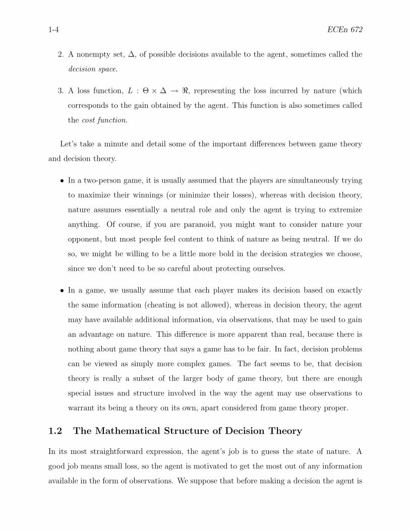
2. A nonempty set, ∆, of possible decisions available to the agent, sometimes called the
decision space.
3. A loss function, L : Θ × ∆ → <, representing the loss incurred by nature (which
corresponds to the gain obtained by the agent. This function is also sometimes called
the cost function.
Let’s take a minute and detail some of the important differences between game theory
and decision theory.
• In a two-person game, it is usually assumed that the players are simultaneously trying
to maximize their winnings (or minimize their losses), whereas with decision theory,
nature assumes essentially a neutral role and only the agent is trying to extremize
anything. Of course, if you are paranoid, you might want to consider nature your
opponent, but most people feel content to think of nature as being neutral. If we do
so, we might be willing to be a little more bold in the decision strategies we choose,
since we don’t need to be so careful about protecting ourselves.
• In a game, we usually assume that each player makes its decision based on exactly
the same information (cheating is not allowed), whereas in decision theory, the agent
may have available additional information, via observations, that may be used to gain
an advantage on nature. This difference is more apparent than real, because there is
nothing about game theory that says a game has to be fair. In fact, decision problems
can be viewed as simply more complex games. The fact seems to be, that decision
theory is really a subset of the larger body of game theory, but there are enough
special issues and structure involved in the way the agent may use observations to
warrant its being a theory on its own, apart considered from game theory proper.
1.2 The Mathematical Structure of Decision Theory
In its most straightforward expression, the agent’s job is to guess the state of nature. A
good job means small loss, so the agent is motivated to get the most out of any information
available in the form of observations. We suppose that before making a decision the agent is
Winter 2009 1-5
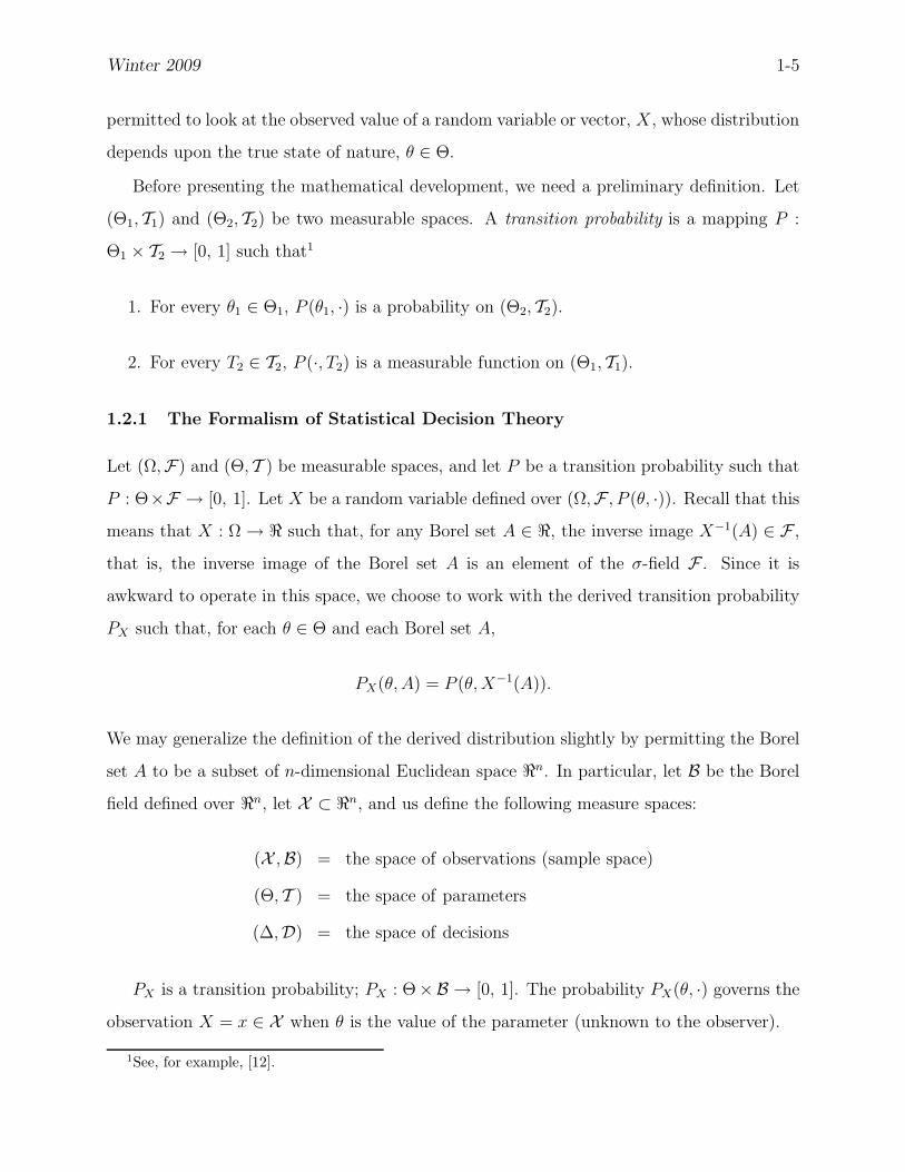
permitted to look at the observed value of a random variable or vector, X, whose distribution
depends upon the true state of nature, θ ∈ Θ.
Before presenting the mathematical development, we need a preliminary definition. Let
(Θ1, T1) and (Θ2, T2) be two measurable spaces. A transition probability is a mapping P :
Θ1 × T2 → [0, 1] such that1
1. For every θ1 ∈ Θ1, P (θ1, ·) is a probability on (Θ2, T2).
2. For every T2 ∈ T2, P (·, T2) is a measurable function on (Θ1, T1).
1.2.1 The Formalism of Statistical Decision Theory
Let (Ω,F) and (Θ, T ) be measurable spaces, and let P be a transition probability such that
P : Θ×F → [0, 1]. Let X be a random variable defined over (Ω,F , P (θ, ·)). Recall that this
means that X : Ω → < such that, for any Borel set A ∈ <, the inverse image X−1(A) ∈ F ,
that is, the inverse image of the Borel set A is an element of the σ-field F . Since it is
awkward to operate in this space, we choose to work with the derived transition probability
PX such that, for each θ ∈ Θ and each Borel set A,
PX(θ, A) = P (θ, X−1(A)).
We may generalize the definition of the derived distribution slightly by permitting the Borel
set A to be a subset of n-dimensional Euclidean space <n. In particular, let B be the Borel
field defined over <n, let X ⊂ <n, and us define the following measure spaces:
(X ,B) = the space of observations (sample space)
(Θ, T ) = the space of parameters
(∆,D) = the space of decisions
PX is a transition probability; PX : Θ×B → [0, 1]. The probability PX(θ, ·) governs the
observation X = x ∈ X when θ is the value of the parameter (unknown to the observer).
1See, for example, [12].

1-6 ECEn 672
Example: Coin Toss. Suppose a coin is tossed, and the agent observes the value X = 1
if it lands “heads,” and X = 0 if it lands “tails.” Then
Ω = H, T
F = ∅, H, T, Ω
The derived Probability space contains the elements
X = 0, 1
B = ∅, 0, 1,X
For a parameter space, let us suppose the coin is either fair or biased towards heads.
Θ = 12, p, p 6= 1
2
T = ∅, 12, p, Θ
Then
PX( 12, A) =
12
A = 0 or A = 11 A = X0 A = ∅
PX(p, A) =
p A = 1(1 − p) A = 01 A = X0 A = ∅
PX(θ, ∅) = 0, all θ ∈ Θ
PX(θ,X ) = 1, all θ ∈ Θ
PX(θ, 1) =
12
θ = 12
p θ = p
PX(θ, 0) =
12
θ = 12
1 − p θ = p
We continue with the development of our formalism; for brevity, we will assume that Bis the Borel field over <. The extension of the concepts to the multivariate case is straight-
forward but lengthy2. For each value of θ ∈ Θ the probability measure PX(θ, ·) induces a
2The definition of a distribution function in the multivariate case is somewhat technical; we won’t dwellon it in this class since we will usually be working with well-known densities. For a detailed treatment ofthe theory, the reader is referred to [17].
Winter 2009 1-7
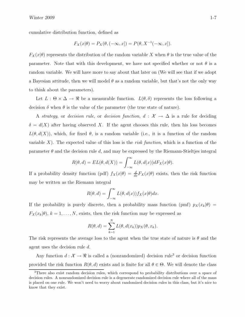
cumulative distribution function, defined as
FX(x|θ) = PX(θ, (−∞, x]) = P (θ, X−1(−∞, x]).
FX(x|θ) represents the distribution of the random variable X when θ is the true value of the
parameter. Note that with this development, we have not specified whether or not θ is a
random variable. We will have more to say about that later on (We will see that if we adopt
a Bayesian attitude, then we will model θ as a random variable, but that’s not the only way
to think about the parameters).
Let L : Θ × ∆ → < be a measurable function. L(θ, δ) represents the loss following a
decision δ when θ is the value of the parameter (the true state of nature).
A strategy, or decision rule, or decision function, d : X → ∆ is a rule for deciding
δ = d(X) after having observed X. If the agent chooses this rule, then his loss becomes
L(θ, d(X)), which, for fixed θ, is a random variable (i.e., it is a function of the random
variable X). The expected value of this loss is the risk function, which is a function of the
parameter θ and the decision rule d, and may be expressed by the Riemann-Stieltjes integral
R(θ, d) = EL(θ, d(X)) =
∫ ∞
−∞L(θ, d(x))dFX(x|θ).
If a probability density function (pdf) fX(x|θ) = ddx
FX(x|θ) exists, then the risk function
may be written as the Riemann integral
R(θ, d) =
∫ ∞
−∞L(θ, d(x))fX(x|θ)dx.
If the probability is purely discrete, then a probability mass function (pmf) pX(xk|θ) =
FX(xk|θ), k = 1, . . . , N , exists, then the risk function may be expressed as
R(θ, d) =
N∑
k=1
L(θ, d(xk))pX(θ, xk).
The risk represents the average loss to the agent when the true state of nature is θ and the
agent uses the decision rule d.
Any function d : X → < is called a (nonrandomized) decision rule3 or decision function
provided the risk function R(θ, d) exists and is finite for all θ ∈ Θ. We will denote the class
3There also exist random decision rules, which correspond to probability distributions over a space ofdecision rules. A nonrandomized decision rule is a degenerate randomized decision rule where all of the massis placed on one rule. We won’t need to worry about randomized decision rules in this class, but it’s nice toknow that they exist.

1-8 ECEn 672
of all nonrandomized decision rules by D. We state without proof that D contains only
functions d for which L(θ, d(·)) is continuous with probability one for each θ ∈ Θ.
With the introduction of the risk function, R, and the class of decision functions, D,
we may replace the original game (Θ, ∆, L) by a new game, which we will denote by the
triple (Θ, D, R), in which the space D and the function R have have an underlying structure,
depending on ∆ and L and the distribution of X, whose exploitation is the main objective
of decision theory. Sometimes the triple (Θ, D, R) is called a statistical game.
Figure 1-2 illustrates the structure of the decision problem. The parameter space is linked
to the decision space through the risk function, which is the expectation of the loss function.
The parameter space is also linked to the sample space through the transition probability
function, and the sample space is linked to the decision space through the decision function.
Parameter Space(Θ, T )
Decision Space(∆,D)
Sample Space(X ,B)
FX(·|θ)
R = E(L)
d(X) ∈ D
Figure 1-2: Structure of a Statistical Game
Example: Odd or Even. The game of “odd or even” mentioned earlier may be extended
to a statistical decision problem. Suppose that before the game is played the agent is allowed
to ask nature how many fingers it intends to put up and that nature must answer truthfully
with probability 3/4 (hence untruthfully with probability 1/4). The agent therefore observes
a random variable X (the answer nature gives) taking the values of 1 or 2. If θ = 1 is the
true state of nature, the probability that X = 1 is 3/4; that is, P (1, 1) = 3/4. Similarly,

Winter 2009 1-9
P (2, 1) = 1/4. There are exactly four possible functions from X = 1, 2 into ∆ = 1, 2.These are the four decision rules
d1(1) = 1, d1(2) = 1;
d2(1) = 1, d2(2) = 2;
d3(1) = 2, d3(2) = 1;
d4(1) = 2, d4(2) = 2.
Rules d1 and d4 ignore the value of X. Rule d2 reflects the agent’s belief that nature is telling
the truth, and rule d3, that nature is not telling the truth. The risk matrix, given in Figure
1-3, characterizes this statistical game.
−3 9/4
2 3/4
−5/4
−7/4
4
−3
@@
@
DΘ
d1 d2 d3 d4
1
2
Figure 1-3: Risk Matrix for Statistical Odd or Even Game
Exercise 1-3 Verify the contents of the risk matrix for the statistical odd or even game.
1.2.2 Special Cases
The above framework provides a formalism for much of the statistical analysis we will do in
this course. Only a part of statistics is represented by this formalism. We will not discuss
such topics as the choice of experiments, the design of experiments, or sequential analysis.
In each case, however, additional structure could be added to the basic framework to include
these topics, and the problem could be reduced again to a simple game. For example, in
sequential analysis the agent may take observations one at time, paying c units each time he
does so. Therefore a decision rule will have to tell him both when to stop taking observations

1-10 ECEn 672
and what action to take once he has stopped. He will try to choose a decision rule that will
minimize in some sense his new risk, which is defined now as the expected value of the loss
plus the cost.
Most of the body of statistical decision making involves three special cases of the general
game formulation.
1. ∆ consists of two points, ∆ = δ1, δ2. If the decision space consists of only two
elements, the resulting problem is called a hypothesis testing problem. Suppose Θ = <and the loss function is
L(θ, δ1) =
`1 if θ > θ0
0 if θ ≤ θ0
L(θ, δ2) =
0 if θ > θ0
`2 if θ ≤ θ0,
where θ0 is some fixed number and `1 and `2 are positive numbers. With this example,
we would like to take action δ1 if θ ≤ θ0, and action δ2 if θ > θ0.
As a specific example, suppose θ represents the return energy of a radar signal, and
θ0 is the minimum return energy that would correspond to the presence of a target.
Suppose the observed return is of the form
X = θ + ν,
where ν is receiver noise. The essence of our decision problem is to decide whether or
not a target is present. Our decision problem can be stated as follows:
Choose δ1 =⇒ H0 : No Target Present
Choose δ2 =⇒ H1 : Target Present.
In statistical parlance, H0 is termed the null hypothesis, and H1 the alternative hy-
pothesis. With this simple problem, four things can happen:
H0 True, Choose δ1: Target not present, decide target not present: correct decision.
H1 True, Choose δ2: Target present, decide target present: correct decision.

Winter 2009 1-11
H1 True, Choose δ1: Target present, decide target not present: missed detection.
H0 True, Choose δ2: Target not present, decide target present: false alarm.
The space D of decision rules consists of those functions d : X → δ1, δ2 with the
property that PX(θ, d(X) = δi) , i = 1, 2, is well-defined for all values of θ ∈ <. With
this structure in place, the problem then, is to determine the function d. This is were
most of the effort of detection theory is placed. It involves the statistical description of
the random variable ν as well as the criterion one would wish to employ for penalizing
errors. For example, if the cost of missed detections is very high, we might have to live
with a high false alarm rate. Conversely, if the cost of false alarms is high, we may
have to design a detector that gives us a lot of missed detections.
Exercise 1-4 Show that the risk function for this case is
R(θ, d) =
`1P (θ, d(X) = δ1) if θ > θ0
`2P (θ, d(X) = δ2) if θ ≤ θ0.
As noted, there are two types of error possible with this problem. First, if θ > θ0,
P (θ, d(X) = δ1) is the probability of making the error of taking action δ1 when
the true state of nature is greater than θ0. In our radar signal detection context, for
example, this error occurs if a target is present, but the decision rule decides that it is
not present–a missed detection. Such an error is often called a Type I error. Similarly,
for θ ≤ θ0,
P (θ, d(X) = δ2) = 1 − P (θ, d(X) = δ1)
is the probability of making the error of taking action δ2 when we should take action
δ1. This error occurs if we the decision rule claims that a target is present when it is
not. Such an error is termed a Type II error.
2. ∆ consists of k points, ∆ = δ1, δ2, · · · , δk, k ≥ 3. These problems are called multiple
decision problems, or multiple hypothesis testing problems.
3. ∆ consists of the real line, ∆ = <. Such decision problems are referred to as point
estimation of a real parameter. Consider the case were Θ = < and the loss function is

1-12 ECEn 672
given by
L(θ, δ) = c(θ − δ)2,
where c is some positive constant. A decision function, d, in this case is a real-valued
function defined on the sample space, and is often called an estimate of the true un-
known state of nature, θ. It is the agent’s desire to choose the function d to minimize
the risk function
R(θ, d) = cE(θ − d(X))2,
which is c times the mean squared error of the estimate d(X). More generally, we may
wish to estimate some function f(θ) that depends on the value of the parameter θ, in
which case the loss function may assume the form
L(θ, δ) = w(θ)(f(θ) − δ)2.
This criterion is one of the most widely used loss functions in all of classical statistical
engineering analysis, and is the basis for such well-known estimation techniques as the
Wiener filter and the Kalman filter.

Winter 2009 2-1
2 The Multivariate Normal Distribution
The normal distribution is probably the most important one for this course. We first present
the univariate normal (Gaussian) distribution, then use that to derive the multivariate dis-
tribution.
2.1 The Univariate Normal Distribution
We begin our discussion with a brief review of the univariate normal distribution. Let X be
a random variable with a univariate normal distribution. This is an absolutely continuous
distribution whose density, with mean µ and variance σ2, is
fX(x) =1√2πσ
exp
(−(x − µ)2
2σ2
)
,
where σ > 0. This distribution is denoted N (µ, σ2). Recall that the characteristic func-
tion of a random variable is defined as the Fourier transform of the density function. The
characteristic function of the univariate normally distributed random variable is
φX(ω) = E exp(jωX)
=
∫ ∞
−∞ejωxfX(x)dx
= exp(jµω − σ2ω2/2) (2-1)
2.2 Development of The Multivariate Distribution
We now turn our attention to the multivariate case. Let X = [X1, . . . , Xn]T denote a random
vector (i.e., each element Xi of this vector is a random variable). The expectation of a random
vector is the vector of expectations: EX = [EX1, . . . , EXn]T 4. The covariance matrix of a
random vector X = [X1, . . . , Xn]T is defined as the matrix of covariances [Cov (Xi, Xj)] or
Cov X = E(X − EX)(X− EX)T .
We have the following fact:
Theorem 1 Every covariance matrix is symmetric and nonnegative definite. Every sym-
metric and nonnegative definite matrix is a covariance matrix. If Cov X is not positive
definite, then with probability one, X lies in some hyperplane bTX = c, with b 6= 0.
4More generally, the expectation of a random matrix is defined as the matrix of expectations.
2-2 ECEn 672
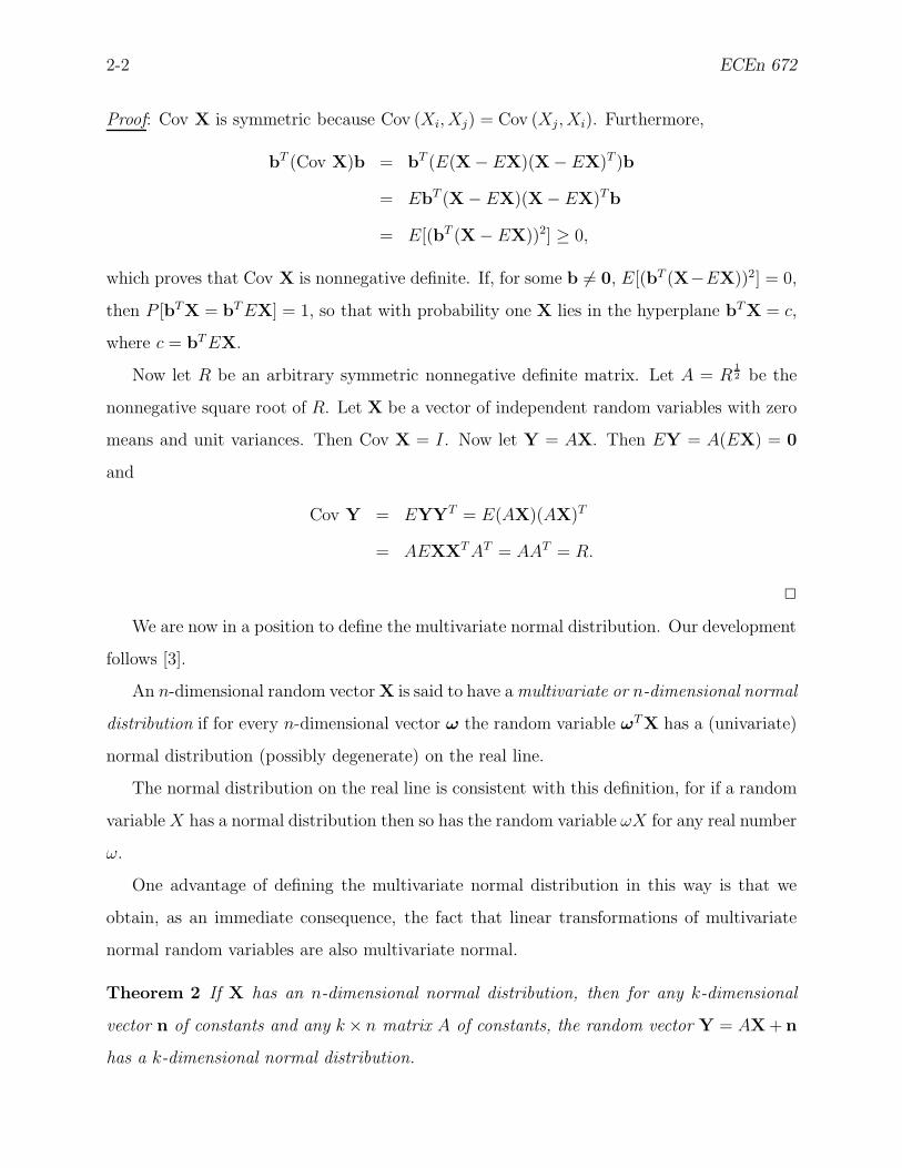
Proof: Cov X is symmetric because Cov (Xi, Xj) = Cov (Xj, Xi). Furthermore,
bT (Cov X)b = bT (E(X − EX)(X− EX)T )b
= EbT (X − EX)(X− EX)Tb
= E[(bT (X − EX))2] ≥ 0,
which proves that Cov X is nonnegative definite. If, for some b 6= 0, E[(bT (X−EX))2] = 0,
then P [bTX = bT EX] = 1, so that with probability one X lies in the hyperplane bTX = c,
where c = bT EX.
Now let R be an arbitrary symmetric nonnegative definite matrix. Let A = R12 be the
nonnegative square root of R. Let X be a vector of independent random variables with zero
means and unit variances. Then Cov X = I. Now let Y = AX. Then EY = A(EX) = 0
and
Cov Y = EYYT = E(AX)(AX)T
= AEXXT AT = AAT = R.
2
We are now in a position to define the multivariate normal distribution. Our development
follows [3].
An n-dimensional random vector X is said to have a multivariate or n-dimensional normal
distribution if for every n-dimensional vector ω the random variable ωTX has a (univariate)
normal distribution (possibly degenerate) on the real line.
The normal distribution on the real line is consistent with this definition, for if a random
variable X has a normal distribution then so has the random variable ωX for any real number
ω.
One advantage of defining the multivariate normal distribution in this way is that we
obtain, as an immediate consequence, the fact that linear transformations of multivariate
normal random variables are also multivariate normal.
Theorem 2 If X has an n-dimensional normal distribution, then for any k-dimensional
vector n of constants and any k × n matrix A of constants, the random vector Y = AX + n
has a k-dimensional normal distribution.
Winter 2009 2-3
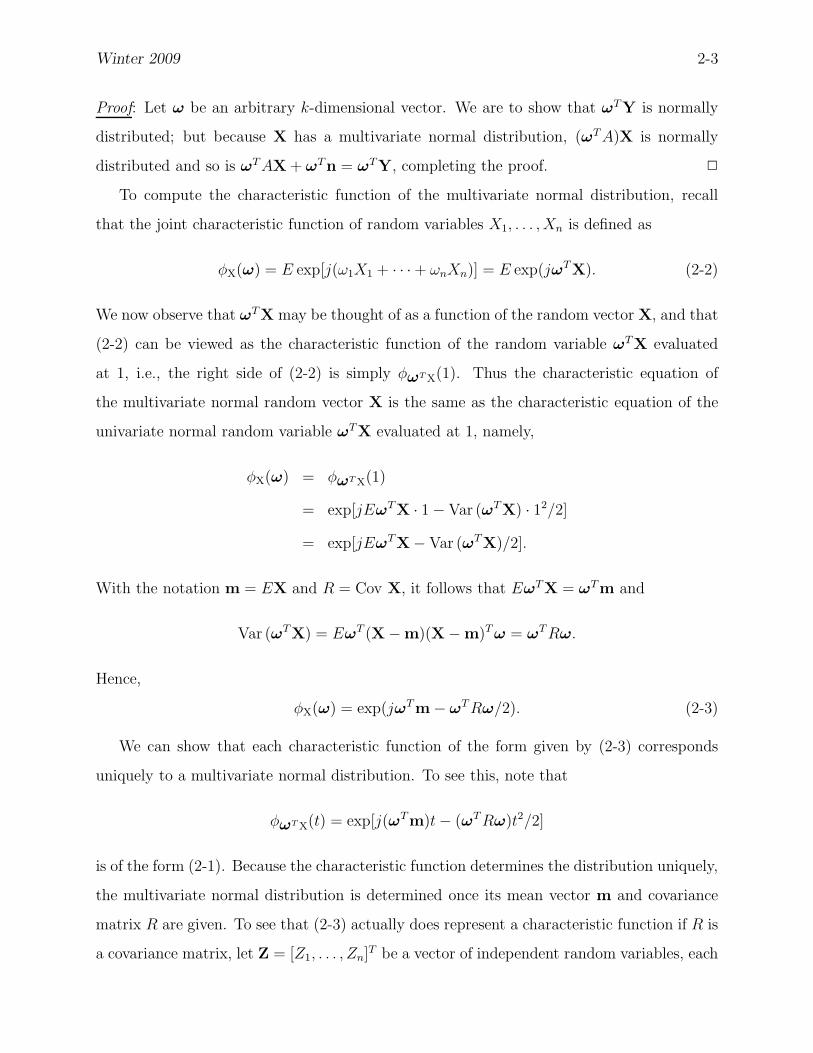
Proof: Let ω be an arbitrary k-dimensional vector. We are to show that ωTY is normally
distributed; but because X has a multivariate normal distribution, (ωT A)X is normally
distributed and so is ωT AX + ωTn = ωTY, completing the proof. 2
To compute the characteristic function of the multivariate normal distribution, recall
that the joint characteristic function of random variables X1, . . . , Xn is defined as
φX(ω) = E exp[j(ω1X1 + · · · + ωnXn)] = E exp(jωTX). (2-2)
We now observe that ωTX may be thought of as a function of the random vector X, and that
(2-2) can be viewed as the characteristic function of the random variable ωTX evaluated
at 1, i.e., the right side of (2-2) is simply φωT X(1). Thus the characteristic equation of
the multivariate normal random vector X is the same as the characteristic equation of the
univariate normal random variable ωTX evaluated at 1, namely,
φX(ω) = φωT X(1)
= exp[jEωTX · 1 − Var (ωTX) · 12/2]
= exp[jEωTX− Var (ωTX)/2].
With the notation m = EX and R = Cov X, it follows that EωTX = ωTm and
Var (ωTX) = EωT (X −m)(X − m)T ω = ωT Rω.
Hence,
φX(ω) = exp(jωTm − ωT Rω/2). (2-3)
We can show that each characteristic function of the form given by (2-3) corresponds
uniquely to a multivariate normal distribution. To see this, note that
φωT X(t) = exp[j(ωTm)t − (ωT Rω)t2/2]
is of the form (2-1). Because the characteristic function determines the distribution uniquely,
the multivariate normal distribution is determined once its mean vector m and covariance
matrix R are given. To see that (2-3) actually does represent a characteristic function if R is
a covariance matrix, let Z = [Z1, . . . , Zn]T be a vector of independent random variables, each
2-4 ECEn 672
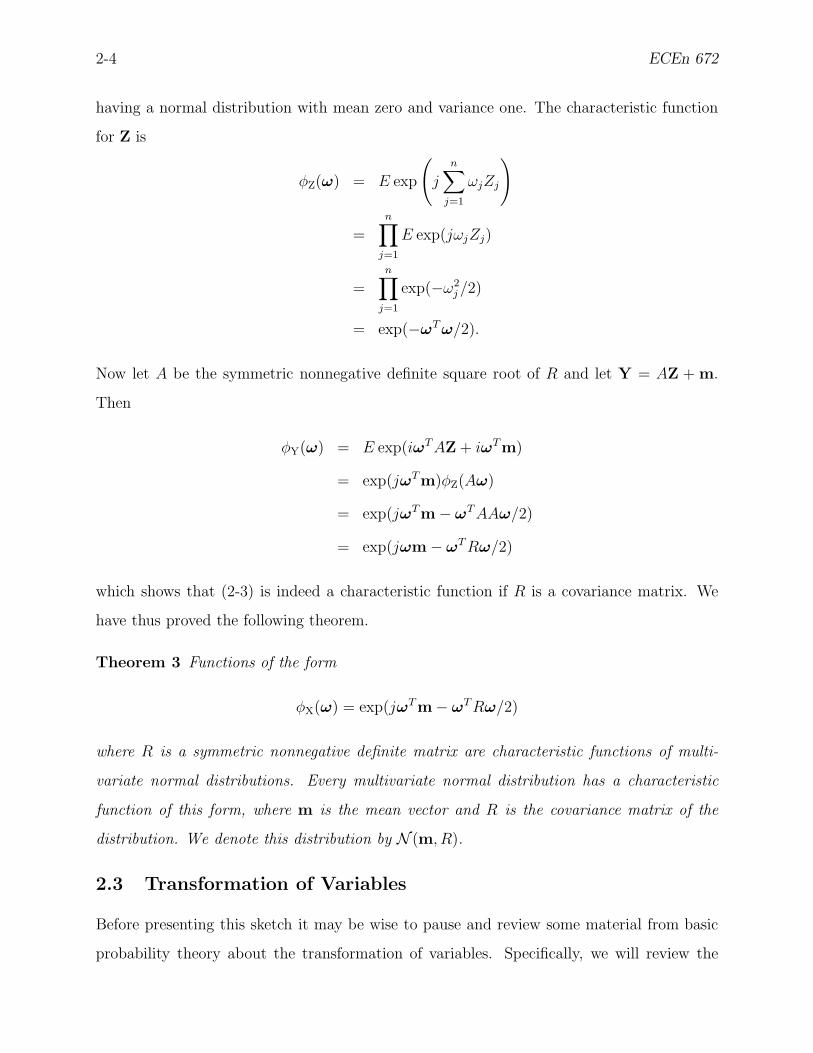
having a normal distribution with mean zero and variance one. The characteristic function
for Z is
φZ(ω) = E exp
(
jn∑
j=1
ωjZj
)
=
n∏
j=1
E exp(jωjZj)
=n∏
j=1
exp(−ω2j /2)
= exp(−ωT ω/2).
Now let A be the symmetric nonnegative definite square root of R and let Y = AZ + m.
Then
φY(ω) = E exp(iωT AZ + iωTm)
= exp(jωTm)φZ(Aω)
= exp(jωTm − ωT AAω/2)
= exp(jωm − ωT Rω/2)
which shows that (2-3) is indeed a characteristic function if R is a covariance matrix. We
have thus proved the following theorem.
Theorem 3 Functions of the form
φX(ω) = exp(jωT m− ωT Rω/2)
where R is a symmetric nonnegative definite matrix are characteristic functions of multi-
variate normal distributions. Every multivariate normal distribution has a characteristic
function of this form, where m is the mean vector and R is the covariance matrix of the
distribution. We denote this distribution by N (m, R).
2.3 Transformation of Variables
Before presenting this sketch it may be wise to pause and review some material from basic
probability theory about the transformation of variables. Specifically, we will review the
Winter 2009 2-5
technique required to calculate the distribution of a function of a random variable. Rather
than prove the general case directly, let’s first prove the univariate case, then state the
general multivariate case.
Theorem 4 Let X and Y be continuous random variables with Y = g(X). Suppose g is
one-to-one and both g and its inverse function, g−1, are continuously differentiable. Then
fY (y) = fX [g−1(y)]
∣∣∣∣
dg−1(y)
dy
∣∣∣∣. (2-4)
Proof. Since g is one-to-one, it is either increasing or decreasing; suppose it is increasing.
Let a and b be real numbers such that a < b; we have
P [Y ∈ (a, b)] = P [g(X) ∈ (a, b)] = P [X ∈ (g−1(a), g−1(b))].
But
P [Y ∈ (a, b)] =
∫ b
a
fY (y)dy
and
P [X ∈ (g−1(a), g−1(b))] =
∫ g−1(b)
g−1(a)
fX(x)dx
=
∫ b
a
fX [g−1(y)]
∣∣∣∣
dg−1(y)
dy
∣∣∣∣dy.
Thus, for all intervals (a, b), we have that∫ b
a
[
fY (y)dy − fX [g−1(y)]
∣∣∣∣
dg−1(y)
dy
∣∣∣∣
]
dy = 0. (2-5)
Suppose that (2-4) is not true. then there exists some y∗ such that equality does not hold;
but by the continuity of the density functions fX and fY , then (2-5) must be nonzero for some
small interval containing y∗. This yields a contradiction, so (2-4) is true if g is increasing.
To show that it holds for decreasing g, we simply note that, the change of variable will also
reverse the limits as well as the sign of slope. Thus, the absolute value will be required. 2
Theorem 5 Let X and Y be continuous random vectors with Y = g(X). Suppose g is
one-to-one and both g and its inverse function, g−1, are both continuously differentiable.
Then
fY(y) = fX[g−1(y)]
∣∣∣∣
∂g−1(y)
∂y
∣∣∣∣, (2-6)
2-6 ECEn 672
where
∣∣∣∣
∂g−1(y)∂y
∣∣∣∣is the absolute value of the Jacobian determinant.
The proof of this theorem is similar to the proof for the univariate case, and we will not
repeat it here.
2.4 The Multivariate Normal Density
It remains to determine the probability density function of a multivariate normally dis-
tributed random vector. We first observe that if R is not positive definite, then all of the
probability mass lies in some hyperplane, and the probability density does not exist. In such
a case, we say that the multivariate normal distribution is singular. When R > 0, however,
the multivariate probability density does exist and is given by the following theorem.
Theorem 6 If the covariance matrix R is nonsingular, the density of the multivariate nor-
mal distribution with characteristic function
φY(ω) = exp(jωTm − ωT Rω/2)
exists and is given by
fY(y) = (2π)−n2 (det R)−
12 exp
− 1
2(y − m)T R−1(y − m)
. (2-7)
Proof: The distribution with characteristic function (2-3) is the distribution of Y = AZ+m
where A is the symmetric positive definite square root of R and were Z ∈ N (0, I). The
density of Z is the product of the marginal densities
fZ(z) = fZ1(z1) · · ·fZn(zn) = (2π)−n2 exp(−zT z/2).
The next step is to determine the density of Y in terms of the density of Z. To do this,
recall the transformation of variables formula, and note that the inverse transform for this
problem is Z = A−1(Y − m), whose Jacobian is
det J = det
(∂Zi
∂Yj
)
= det A−1 = det R− 12 = (det R)−
12 .
Hence, the density of Y is
fY(y) = fZ(A−1(y − m)) det J
= (2π)−n2 (det R)−
12 exp[− 1
2(y − m)T A−1A−1(y −m)]

Winter 2009 2-7
which reduces to (2-7). 2
We complete our discussion of multivariate normal distributions by noting that, while the
covariance of two independent random variables is zero, a zero covariance does not generally
imply that the variables are independent. For the multivariate normal distribution, however,
zero covariance does imply independence.
Theorem 7 If Y ∈ N (m, R), then the component random variables Y1, . . . , Yn are mutually
independent if and only if R is a diagonal matrix.
Proof: If R is not diagonal, then there is a nonzero off-diagonal element which gives a
nonzero covariance between two of the elements of Y; therefore they cannot be independent.
Conversely, if R = diag σ21, . . . , σ
2n, the characteristic function factors as
φY(ω) = exp
(
i
n∑
j=1
ωjmj − 12
n∑
j=1
ωjσ2j
)
=n∏
j=1
exp(jωjmj − 12ωjσ
2j ),
which proves the independence. 2
Exercise 2-1 Let Y = AX + µ be a linear transformation from X to Y, where A is a
nonsingular square matrix and µ is a constant vector. Show that the Jacobian det(
∂yi
∂xj
)
of
this transformation is the determinant of A.
Exercise 2-2 (Ferguson) Random variables may be univariate normal but not jointly nor-
mal. Here is an example of two normal random variables that are uncorrelated but not
independent. Let X have a normal distribution with mean zero and variance one. Let c be
a nonnegative number and let Y = −X if |X| ≤ c and Y = X if |X| > c. Then Y also
has a normal distribution with zero mean and variance one. Show that the covariance of
X and Y is a continuous function of c, going from +1, when c = 0, to −1 when c → ∞.
Therefore for some value of c, X and Y are uncorrelated, yet X and Y are are as far from
being independent as possible, each being a function of the other. (c = 1.538 · · · ).

Winter 2009 3-1
3 Introductory Estimation Theory Concepts
3.1 Notational Conventions
In an earlier disucssion we introduced the transition probability P (θ, ·), and observed that,
for every value of θ, this function is a probability. For a given random variable, X, we
then formed the derived distribution, which we expressed as PX(θ, ·), and we expressed the
associated distribution function as FX(x | θ) with corresponding notational conventions for
the probability density function (pdf) and probability mass function (pmf). Although most
of our work will involve the distribution and, as appropriate, the pdf or pmf, it will often
be necessary to refer to the transition probability function P (θ, ·). When there is no chance
of confusion concerning the random variable under consideration, it is customary to adopt
abbreviated notation. Two such notational conventions are common. Sometimes we will
write Pθ(·) to denote this probability, and sometimes we will write it as P (·|θ). In both
cases, we depend on the identity of the random variable to be understood from the context
of the problem. You will need to get used to both notations, as they will both appear in the
literature and in these notes5.
When there is no likelihood of confusion, we may also sometimes denote the distribution
function FX(x | θ) by the abbreviated form Fθ(x). For discrete random variables, the proba-
bility mass function (pmf) will be denoted by fX(x | θ) or fθ(x) and, similarly, for continuous
random variables, the probability density function (pdf) will also be denoted by fX(x | θ) or
fθ(x).
We will also be required to take the mathematical expectation of various random vari-
ables. As usual, we let E(·) denote the expectation operator (with or without parentheses,
depending upon the chances of confusion). When we write EX it is understood that this
expectation is performed using the distribution function of X, but when this distribution
function is parameterized by θ, we must augment this notation by writing EθX.
5I think it one of the unspoken prerogatives of probabilists and statisticians to use arcane, inconsistentand, sometimes, abusive notation.
3-2 ECEn 672
3.2 Populations and Statistics
As we have described earlier, the problem of estimation is, essentially, to obtain a set of
data, or observations, and use this information in some way to fashion a guess for the value
of an unknown parameter (the parameter may be a vector). One of the ways to achieve this
goal is through the method of random sampling. Our starting point for this discussion is
the concept of a population.
Definition. A population, or parent population, is the probability space (<,B, PX(θ, ·)) in-
duced on < by a random variable X. The random variable X is called the population random
variable. The distribution of the population is the distribution of X. The population is dis-
crete or continuous according as X is discrete or continuous. This definition extends to the
vector case in the obvious way.
By sampling, we mean that we repeat a given experiment a number times; The ith
repetition involves the creation, mathematically, of a replica, or copy, of the population on
which a random variable Xi is defined. The distribution of the random variable Xi is the
same as the distribution of X, the parent population random variable. The random variables
X1, X2, . . . , are called sample random variables or, sometimes, the sample values of X. In
general, a function of the sample values of a random variable X is called a statistic of X.
The act of sampling can take many forms, some of which will be discussed in this course.
Perhaps the simplest sampling procedure is that of sampling with replacement. A more
complicated sampling example involves the sampling of an entire stochastic process.
For an example of sampling with replacement, let X be a random variable with unknown
mean value. Suppose we have a collection of independent samples of X, which we will denote
as X1, . . . , Xn. The sample mean, written as the random variable X, is given by
X =1
n
n∑
i=1
Xi,
and is an example of an estimator of the population mean; that is, X is a statistic.
Before continuing with this discussion, it is important to make a distinction between
random variables and the values they may take. Once the observations have been taken, the
sample values become evaluated at the points Xi = xi, and the array x1, . . . , xn; that is

Winter 2009 3-3
X = xi is a collection of real numbers. After the observations, therefore, the sample mean
may be evaluated as
x =1
n
n∑
i=1
xi.
The real number x is not a random variable, nor are the quantities x1, . . . xn. When we talk
about quantities such as the mean or variance, they are associated with random variables,
and not the values they assume. We can certainly talk about the average of the numbers
x1, . . . , xn, but this average is not the mathematical expectation of the random variable X.
The only way we can think of x as a random variable is in a degenerate sense, where all of
the mass is located at the number x. Outside this context, it is meaningless to speak of the
mean or variance of x, but it is highly relevant to speak of the mean and variance of the
random variable X.
3.2.1 Sufficient Statistics
The random variable, X, is one of many possible statistics to be obtained from the samples
X1, . . . , Xn. Suppose our objective in collecting the observations is to determine the mean
value of the random variable X. Let us ask ourselves, What information about X is furnished
by the sample values? Or perhaps better, What is the best estimate of the mean value of
X that we can make on the basis of the sample values alone? This question is not yet
really mathematically meaningful, since the notion of “best” has not been defined. Yet,
with the above example, there is a strong compulsion to suppose that the random variable,
X, captures everything there is to learn from the random variables X1, . . . , Xn about the
expectation of X. As we will see, the random variable X contains some special properties
that qualify it as a sufficient statistic for the mean of the random variable X.
Definition. Let X be a random variable whose distribution depends on a parameter θ. A
real-valued function T of X is said to be sufficient for θ if the conditional distribution of X,
given T = t, is independent of θ. That is, T is sufficient for θ if
FX|T (x | t, θ) = FX|T (x | t).
The above definition remains unchanged if X, θ, and T are vector-valued, rather than
scalar-valued.
3-4 ECEn 672
Example 3-1 A coin with unknown probability p, 0 ≤ p ≤ 1, of heads is tossed indepen-
dently n times. If we let Xi be zero if the outcome of the ith toss is tails and one if the outcome
is heads, the random variables X1, . . . , Xn are independent and identically distributed with
common probability mass function
fX(xi | p) = P (Xi = xi | p) = pxi(1 − p)1−xi for xi = 0, 1.
If we are looking at the outcome of this sequence of tosses in order to make a guess of the
value of p, it is clear that the important thing to consider is the total number of heads and
tails. It is hard to see how the information concerning the order of heads and tails can help
us once we know the total number of heads. In fact, if we let T denote the total number
of heads, T =∑n
i=1 Xi, then intuitively the conditional distribution of X1, . . . , Xn, given
T = j, is uniform over the
(nj
)
n-tuples which have j ones and n − j zeros; that is,
given that T = j, the distribution of X1, . . . , Xn may be obtained by choosing completely at
random the j places in which ones go and putting zeros in the other locations. This may be
done not knowing p. Thus, once we know the total number of heads, being given the rest of
the information about X1, . . . , Xn is like being told the value of a random variables whose
distribution does not depend on p at all. In other words, the total number of heads carries
all the information the sample has to give about the unknown parameter p. We claim that
the total number of heads is a sufficient statistic for p.
To prove that fact, we need to show that the conditional distribution of X1, . . . , Xn,given T = t, is independent of p. This conditional distribution is
fX1,...Xn | T (x1, . . . , xn | t, p) =P (X1 = x1, . . .Xn = xn, T = t | p)
P (T = t | p). (3-1)
The denominator of this expression is the binomial probability
P (T = t | p) =
(nt
)
pt(1 − p)n−t. (3-2)
We now examine the numerator. Since t represents the sum of the values Xi takes, we must
set the probability that X1 + . . . + Xn 6= t to zero, otherwise we will have an inconsistent
probability. Thus, the numerator is zero except when x1 + . . . + xn = t and each xi = 0 or 1,
Winter 2009 3-5
and then
P (X1 = x1, . . . , Xn = xn, T = t | p) = P (X1 = x1, . . . , Xn = xn | p)
= px1(1 − p)1−x1 . . . pxn(1 − p)1−xn
= pP
xi(1 − p)n−P
xi . (3-3)
But t =∑
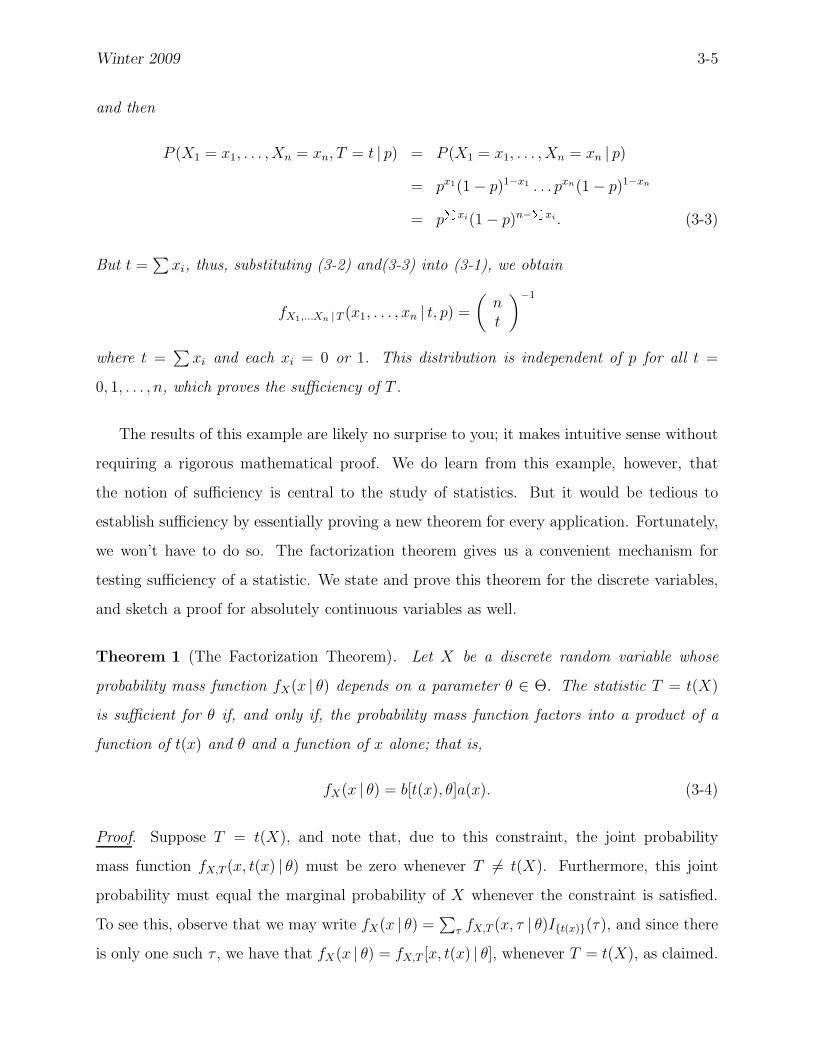
xi, thus, substituting (3-2) and(3-3) into (3-1), we obtain
fX1,...Xn |T (x1, . . . , xn | t, p) =
(nt
)−1
where t =∑
xi and each xi = 0 or 1. This distribution is independent of p for all t =
0, 1, . . . , n, which proves the sufficiency of T .
The results of this example are likely no surprise to you; it makes intuitive sense without
requiring a rigorous mathematical proof. We do learn from this example, however, that
the notion of sufficiency is central to the study of statistics. But it would be tedious to
establish sufficiency by essentially proving a new theorem for every application. Fortunately,
we won’t have to do so. The factorization theorem gives us a convenient mechanism for
testing sufficiency of a statistic. We state and prove this theorem for the discrete variables,
and sketch a proof for absolutely continuous variables as well.
Theorem 1 (The Factorization Theorem). Let X be a discrete random variable whose
probability mass function fX(x | θ) depends on a parameter θ ∈ Θ. The statistic T = t(X)
is sufficient for θ if, and only if, the probability mass function factors into a product of a
function of t(x) and θ and a function of x alone; that is,
fX(x | θ) = b[t(x), θ]a(x). (3-4)
Proof. Suppose T = t(X), and note that, due to this constraint, the joint probability
mass function fX,T (x, t(x) | θ) must be zero whenever T 6= t(X). Furthermore, this joint
probability must equal the marginal probability of X whenever the constraint is satisfied.
To see this, observe that we may write fX(x | θ) =∑
τ fX,T (x, τ | θ)It(x)(τ), and since there
is only one such τ , we have that fX(x | θ) = fX,T [x, t(x) | θ], whenever T = t(X), as claimed.

3-6 ECEn 672
Assume that T is sufficient for θ, and that T = t(X). Then the conditional distribution
of X given T is independent of θ, and we may write
fX(x | θ) = fX,T [x, t(x) | θ]
= fX|T [x | t(x), θ]fT [t(x) | θ]
= fX|T [x | t(x)]fT [t(x) | θ],
provided the conditional probability is well defined. Hence, we define a(x) by
a(x) =
0 if fX(x | θ) = 0 for all θ ∈ Θ
fX|T [x | t(x)] if fX(x | θ) > 0 for some θ ∈ Θ.
With
b[t(x), θ] = fT [t(x) | θ],
the factorization is established.
To establish the converse, suppose a factorization of the form (3-4) holds, and let t0 be
chosen such that fT (t0 | θ) > 0 for some θ ∈ Θ. Then
fX|T (x | t0, θ) =fX,T (x, t0 | θ)
fT (t0 | θ). (3-5)
The numerator is zero for all θ whenever t(x) 6= t0, and when t(x) = t0, the numerator is
simply fX(x | θ), by our previous argument. The denominator may be written
fT (t0 | θ) =∑
x∈A(t0)
fX(x | θ)
=∑
x∈A(t0)
b[t(x), θ]a(x), (3-6)
where A(t0) = x : t(x) = t0. Hence, substituting (3-4) and (3-6) into (3-5) and setting the
pmf to zero otherwise, we obtain
fX|T (x | t0, θ) =
0 if t(x) 6= t0b(t0, θ)a(x)
b(t0, θ)∑
x′∈A(t0)
a(x′)if t(x) = t0
Thus, fX|T (x | t0) is independent of θ for all t0 and θ for which it is defined. 2

Winter 2009 3-7
The factorization theorem is also true for a large family of continuous random variables.
A completely rigorous proof is outside the scope of this class, but we will give a sketch of
the proof, which will hopefully illuminate the key things that go on, and give you confidence
that the result is true.
Armed with an understanding of the transformation of variables theorem, we may now
sketch a proof of the factorization theorem for the continuous case.
Sketch of the proof in the absolutely continuous case. For this development we recognize that
the statistic may be multi-dimensional, so we generalize the treatment to permit vector-
valued statistics, which we will denote by T. We first observe that the statistic T may not
be a one-to-one mapping of the random vector X, since the dimension of T may be different
from the dimension of X. A standard trick when dealing with problems of this type is to
include some additional functions in order to fill out the dimension of the transformation.
For example, if T is r-dimensional, then the dimension of U would be n− r. We then prove
the theorem with the aid of these auxiliary functions and finally show that the choice of
functions does not matter to the result we want. This approach may seem a little messy, but
unless we do something to enable us to use our standard transformation of variables formula
the proof is likely to be even more messy.
So, let U(X) be an auxiliary statistic so that the mapping
X = g(T,U)
is one-to-one and therefore invertible. Further, suppose U is smooth enough for the Jaco-
bian to exist. Notation becomes a problem with manipulations of this kind, and it will be
convenient to write x(t,u) for g(t,x), and (t(x),u(x)) for g−1(x). The densities transform
as follows:
fX(x | θ) = fg(X)[g−1(x), | θ]
∣∣∣∣
∂g−1(x)
∂x
∣∣∣∣
= fT,U[t(x),u(x) | θ]∣∣∣∣
∂(t(x),u(x))
∂x
∣∣∣∣
= fT[t(x) | θ]fU|T[u(x) | t(x), θ]
∣∣∣∣
∂(t(x),u(x))
∂x
∣∣∣∣,
where
∣∣∣∣
∂(t(x),u(x))∂x
∣∣∣∣
is the absolute value of the Jacobian determinant. If T is sufficient,

3-8 ECEn 672
then fU|T(u | t, θ) is independent of θ, giving the required factorization analogous to the
earlier proof.
Conversely, if a factorization exists, then
fT,U(t,u | θ) = fX[g(t,u) | θ]∣∣∣∣
∂g(t,u)
∂(t,u)
∣∣∣∣
= fX[x(t,u) | θ]∣∣∣∣
∂x(t,u)
∂(t,u)
∣∣∣∣
= b(t, θ)a[x(t,u)]
∣∣∣∣
∂x(t,u)
∂(t,u)
∣∣∣∣, (3-7)
so that, integrating out the u, the marginal of T becomes
fT(t | θ) = b(t, θ)
∫
a[x(t,u)]
∣∣∣∣
∂x(t,u)
∂(t,u)
∣∣∣∣du, (3-8)
and we have, taking the ratio of (3-7) and (3-8),
fU|T(u, θ) =fT,U(t,u | θ)
fT(t | θ)
=
a[x(t,u)]
∣∣∣∣
∂x(t,u)∂(t,u)
∣∣∣∣
∫a[x(t,u)]
∣∣∣∣
∂x(t,u)∂(t,u)
∣∣∣∣du
,
independent of θ. Thus the distribution of U given T is independent of θ; hence the distribu-
tion of (T,U) given T is independent of θ, and the distribution of X, given T, is independent
of θ. 2
Example 3-2 Consider a sample X1, . . . , Xn from N (µ, σ2). The joint density of X1, . . . , Xn
is
fX1,...,Xn(x1, . . . , xn |µ, σ) = (2πσ2)−n2 exp[−(2σ2)−1
n∑
i=1
(xi − µ)2]. (3-9)
If µ is a known quantity, then from the factorization theorem t(X) =∑n
i=1(Xi − µ)2 is a
sufficient statistic for σ2. (In this case the function a(x) may be taken identically equal to
one.) Let x = 1n
∑ni=1 xi and s2 = 1
n
∑ni=1(xi − x)2, so that the density (3-9) may be written
fX1,...,Xn(x1, . . . , xn |µ, σ) = (2πσ2)−n2 exp[−ns2/2σ2] · exp[−n(x − µ)2/2σ2].
If σ2 is a known quantity, then from the factorization theorem, X is a sufficient statistic for
µ. If both µ and σ2 are unknown, the pair (X, S2) is a sufficient statistic for (µ, σ2). (We

Winter 2009 3-9
adopt the notation that X and S2 are the random variables corresponding to the realizations
x and s2.)
Example 3-3 Consider a sample X1, . . . , Xn from the uniform distribution over the interval
[α, β]. The joint density is
fX1,...,Xn(x1, . . . , xn |α, β) = (β − α)−n
n∏
i=1
I(α,β)(xi),
where IA is the indicator function: IA(x) = 1 if x ∈ A, IA(x) = 0 if x 6∈ A. This joint
density may be rewritten as
fX1,...,Xn(x1, . . . , xn |α, β) = (β − α)−nI(α,∞)(min xi)I(−∞,β)(max xi).
We examine three cases. First, if α is known, then max Xi is a sufficient statistic for β.
Second, if β is known, then min Xi is a sufficient statistic for α, and if both α and β are
unknown, then (min Xi, max Xi) is a sufficient statistic for (α, β).
3.2.2 Complete Sufficient Statistics
As we have seen, the concept of a sufficient statistic is useful for simplifying the structure of
estimators. It leads to economy in the design of algorithms to compute the estimates, and
may simplify the requirements for data acquisition and storage. Clearly, not all sufficient
statistics are created equal. As an extreme case, the mapping T1(X1, . . . , Xn) = (X1, . . . , Xn)
is always sufficient statistic, but no reduction in complexity is obtained. At the other extreme,
if the random variables Xi are i.i.d., then, as we have seen, a sufficient statistic for the mean
is the average, T2(X1, . . . , Xn) = X, and it is hard to see how complexity could be reduced
further. What about the vector-valued statistic T3(X1, . . . , Xn) =(∑n−1
i=1 Xi, Xn
)? It is
straightforward that this statistic is also sufficient for the mean. Obviously, T2 would be
require less bandwidth to transmit, less memory to store, and would be simpler to use, but
all three are sufficient for the mean. In fact, it easy to see that T3 can be expressed as
function of T1 but not vice versa, and that T2 can be expressed as a function of T3 (and,
consequently, of T1). This leads to a useful definition.
Definition. A sufficient statistic for a parameter θ ∈ Θ that is a function of all other sufficient
statistics for θ is said to be a minimal sufficient statistic, or necessary and sufficient statistic,
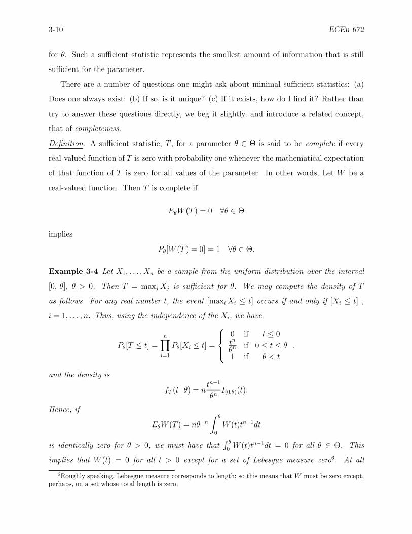
3-10 ECEn 672
for θ. Such a sufficient statistic represents the smallest amount of information that is still
sufficient for the parameter.
There are a number of questions one might ask about minimal sufficient statistics: (a)
Does one always exist: (b) If so, is it unique? (c) If it exists, how do I find it? Rather than
try to answer these questions directly, we beg it slightly, and introduce a related concept,
that of completeness.
Definition. A sufficient statistic, T , for a parameter θ ∈ Θ is said to be complete if every
real-valued function of T is zero with probability one whenever the mathematical expectation
of that function of T is zero for all values of the parameter. In other words, Let W be a
real-valued function. Then T is complete if
EθW (T ) = 0 ∀θ ∈ Θ
implies
Pθ[W (T ) = 0] = 1 ∀θ ∈ Θ.
Example 3-4 Let X1, . . . , Xn be a sample from the uniform distribution over the interval
[0, θ], θ > 0. Then T = maxj Xj is sufficient for θ. We may compute the density of T
as follows. For any real number t, the event [maxi Xi ≤ t] occurs if and only if [Xi ≤ t] ,
i = 1, . . . , n. Thus, using the independence of the Xi, we have
Pθ[T ≤ t] =
n∏
i=1
Pθ[Xi ≤ t] =
0 if t ≤ 0tn
θn if 0 ≤ t ≤ θ
1 if θ < t
,
and the density is
fT (t | θ) = ntn−1
θnI(0,θ)(t).
Hence, if
EθW (T ) = nθ−n
∫ θ
0
W (t)tn−1dt
is identically zero for θ > 0, we must have that∫ θ
0W (t)tn−1dt = 0 for all θ ∈ Θ. This
implies that W (t) = 0 for all t > 0 except for a set of Lebesgue measure zero6. At all
6Roughly speaking, Lebesgue measure corresponds to length; so this means that W must be zero except,perhaps, on a set whose total length is zero.

Winter 2009 3-11
points of continuity, the fundamental theorem of calculus shows that W (t) is zero. Hence,
Pθ[W (T ) = 0] = 1 for all θ > 0, so that T is a complete sufficient statistic.
Our interest in forming the notion of completeness is that it has some useful consequences.
In particular, we present two of the most important properties of complete sufficient statistics.
We precede these properties by an important definition.
Definition. Let X be a random variable whose sample values are used to estimate a parameter
θ of the distribution of X. An estimate θ(X) of a θ is said to be unbiased if, when θ is the
true value of the parameter, the mean of the distribution of θ(X) is θ, i.e.,
Eθθ(X) = θ ∀θ.
Theorem 2 (Lehmann-Scheffe). Let T be a complete sufficient statistic for a parameter
θ ∈ Θ, and let W be a function of T that produces an unbiased estimate of θ; then W is
unique with probability one.
Proof. Let W1 and W2 be two functions of T that produce unbiased estimates of θ. Thus,
EθW1(T ) = EθW2(T ) = θ ∀θ ∈ Θ.
But then
Eθ[W1(T ) − W2(T )] = 0 ∀θ ∈ Θ.
We note, however, that W1(T ) − W2(T ) is a function of T , so by the completeness of T , we
must have W1(T ) − W2(T ) = 0 with probability one for all θ ∈ Θ. 2
Theorem 3 A complete sufficient statistic for a parameter θ ∈ Θ is minimal.
Before proving this theorem, we need the following background material.
Definition. Let F be a σ-field, and let X be a random variable such that E|X| < ∞. The
conditional expectation of X given F is a random variable, written as
EFX or E(X|F),
such that it possesses the following attributes:

3-12 ECEn 672
(a) E(X|F) is an F -measurable random variable, and
(b) E[X − E(X|F)] Z = 0 for all F -measurable random variables Z.
In particular, if Y be a random variable, and F = σY is the σ-field generated by Y , that
is, the σ-field containing the inverse images under Y of all Borel sets, then we write the
conditional expectation as E(X|Y ).
Attribute (b) of the conditional expectation is the one that makes it useful. It says that
the random variable X −E(X|F) is orthogonal to all random variables that are measurable
with respect to F . Hence, if F = σY , then the difference between the random variable
X and its conditional expectation given Y is orthogonal to Y . We will develop these ideas
more fully later in the course.
The following list enumerates the main properties of conditional expectations.
1. E(X|Y ) = EX if X and Y are independent.
2. EX = E[E(X|Y )].
3. E(X|Y ) = f(Y ), where f(·) is a function.
4. E[g(Y )X|Y ] = g(Y )E(X|Y ), where g(·) is a function.
5. If Z is a random variable and σY ⊂ σZ, then E(X|Y ) = E[E(X|Z)|Y ].
6. If Z is a random variable and σY ⊂ σZ, then E(X|Y ) = E[E(X|Y )|Z].
7. E(c|Y ) = c for any constant c.
8. E[g(Y )|Y ] = g(Y ).
9. E[(cX + dZ)|Y ] = cE(X|Y ) + dE(Z|Y ) for any constants c and d.
Proof. Let T be a complete sufficient statistic and let S be another sufficient statistic, and
suppose that S is minimal. By Property 2, we know that ET = E[E(T |S)]. By Property
3, we know that the conditional expectation E(T |S) is a function of S. But, because S is
minimal, we also know that S is a function of T . Thus, the random variable T − E(T |S) is
Winter 2009 3-13
a function of T , and this function has zero expectation for all θ ∈ Θ. Therefore, since T is
complete, it follows that T = E(T |S) with probability one. This makes T a function of S,
and since S is minimal, T is therefore a function of all other sufficient statistics, and T is
itself minimal. 2
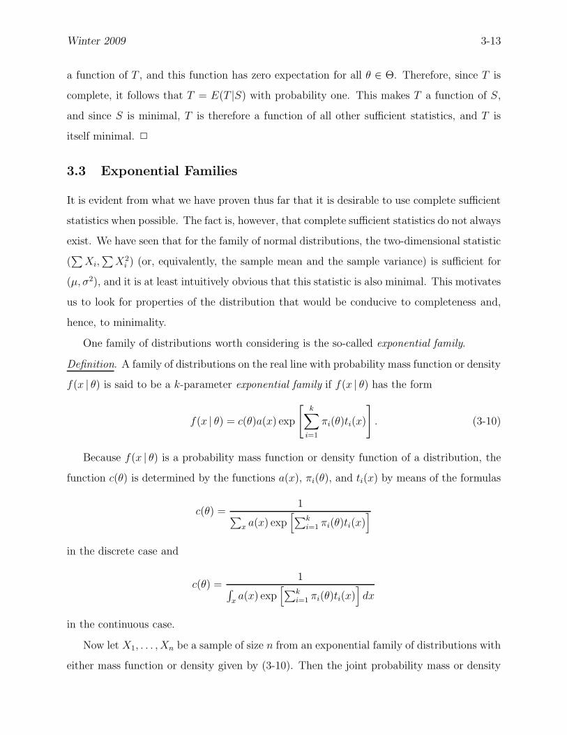
3.3 Exponential Families
It is evident from what we have proven thus far that it is desirable to use complete sufficient
statistics when possible. The fact is, however, that complete sufficient statistics do not always
exist. We have seen that for the family of normal distributions, the two-dimensional statistic
(∑
Xi,∑
X2i ) (or, equivalently, the sample mean and the sample variance) is sufficient for
(µ, σ2), and it is at least intuitively obvious that this statistic is also minimal. This motivates
us to look for properties of the distribution that would be conducive to completeness and,
hence, to minimality.
One family of distributions worth considering is the so-called exponential family.
Definition. A family of distributions on the real line with probability mass function or density
f(x | θ) is said to be a k-parameter exponential family if f(x | θ) has the form
f(x | θ) = c(θ)a(x) exp
[k∑
i=1
πi(θ)ti(x)
]
. (3-10)
Because f(x | θ) is a probability mass function or density function of a distribution, the
function c(θ) is determined by the functions a(x), πi(θ), and ti(x) by means of the formulas
c(θ) =1
∑
x a(x) exp[∑k
i=1 πi(θ)ti(x)]
in the discrete case and
c(θ) =1
∫
xa(x) exp
[∑k
i=1 πi(θ)ti(x)]
dx
in the continuous case.
Now let X1, . . . , Xn be a sample of size n from an exponential family of distributions with
either mass function or density given by (3-10). Then the joint probability mass or density
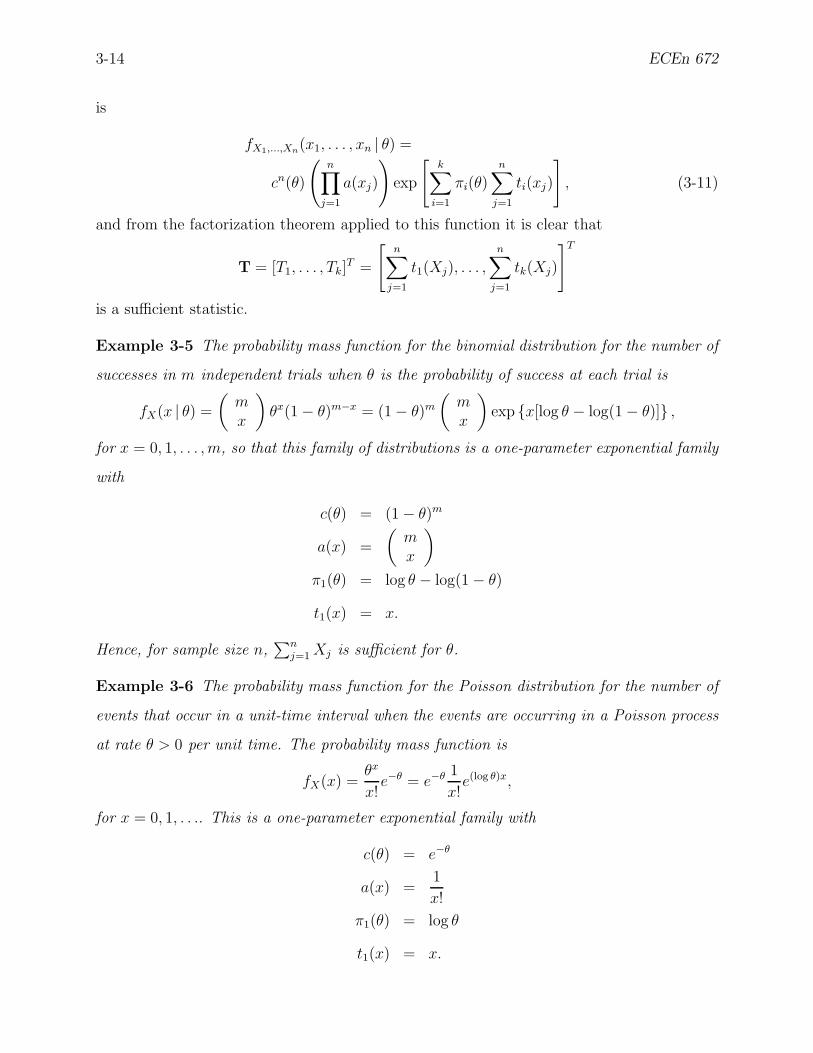
3-14 ECEn 672
is
fX1,...,Xn(x1, . . . , xn | θ) =
cn(θ)
(n∏
j=1
a(xj)
)
exp
[k∑
i=1
πi(θ)n∑
j=1
ti(xj)
]
, (3-11)
and from the factorization theorem applied to this function it is clear that
T = [T1, . . . , Tk]T =
[n∑
j=1
t1(Xj), . . . ,
n∑
j=1
tk(Xj)
]T
is a sufficient statistic.
Example 3-5 The probability mass function for the binomial distribution for the number of
successes in m independent trials when θ is the probability of success at each trial is
fX(x | θ) =
(mx
)
θx(1 − θ)m−x = (1 − θ)m
(mx
)
exp x[log θ − log(1 − θ)] ,
for x = 0, 1, . . . , m, so that this family of distributions is a one-parameter exponential family
with
c(θ) = (1 − θ)m
a(x) =
(mx
)
π1(θ) = log θ − log(1 − θ)
t1(x) = x.
Hence, for sample size n,∑n
j=1 Xj is sufficient for θ.
Example 3-6 The probability mass function for the Poisson distribution for the number of
events that occur in a unit-time interval when the events are occurring in a Poisson process
at rate θ > 0 per unit time. The probability mass function is
fX(x) =θx
x!e−θ = e−θ 1
x!e(log θ)x,
for x = 0, 1, . . .. This is a one-parameter exponential family with
c(θ) = e−θ
a(x) =1
x!
π1(θ) = log θ
t1(x) = x.
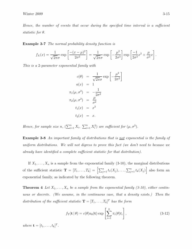
Winter 2009 3-15
Hence, the number of events that occur during the specified time interval is a sufficient
statistic for θ.
Example 3-7 The normal probability density function is
fX(x) =1√2πσ
exp
[−(x − µ)2
2σ2
]
=1√2πσ
exp
[
− µ2
2σ2
]
exp
[−1
2σ2x2 +
µ
σ2x
]
.
This is a 2-parameter exponential family with
c(θ) =1√2πσ
exp
[
− µ2
2σ2
]
a(x) = 1
π1(µ, σ2) = − 1
2σ2
π2(µ, σ2) =µ
σ2
t1(x) = x2
t2(x) = x.
Hence, for sample size n, (∑n
i=1 Xi,∑n
i=1 X2i ) are sufficient for (µ, σ2).
Example 3-8 An important family of distributions that is not exponential is the family of
uniform distributions. We will not digress to prove this fact (we don’t need to because we
already have identified a complete sufficient statistic for that distribution).
If X1, . . . , Xn is a sample from the exponential family (3-10), the marginal distributions
of the sufficient statistic T = [T1, . . . , Tk] =[∑n
j=1 t1(Xj), . . . ,∑n
j=1 tk(Xj)]
also form an
exponential family, as indicated by the following theorem.
Theorem 4 Let X1, . . . , Xn be a sample from the exponential family (3-10), either contin-
uous or discrete. (We assume, in the continuous case, that a density exists.) Then the
distribution of the sufficient statistic T = [T1, . . . , Tk]T has the form
fT(t | θ) = c(θ)a0(t) exp
[k∑
i=1
πi(θ)ti
]
, (3-12)
where t = [t1, . . . , tk]T .

3-16 ECEn 672
Proof in the continuous case. From the proof of the factorization theorem (see (3-8)), we
may write the marginal distribution of T as
fT(t | θ) = b(t, θ)
∫
a[x(t,u)]
∣∣∣∣
∂x(t,u)
∂(t,u)
∣∣∣∣du.
Also, by the factorization theorem, we know that
b[t(x), θ] =fX(x | θ)
a(x)
and, when fX is exponential, we may write
b[t(x), θ] =c(θ)a(x) exp
[∑k
i=1 πi(θ)ti(x)]
a(x),
so, substituting this into the marginal for T, we obtain
fT(t | θ) = c0(θ)
[∫
a[x(t,u)]
∣∣∣∣
∂x(t,u)
∂(t,u)
∣∣∣∣du
]
exp
[∑
i=1
πi(θ)ti
]
,
which is of the desired form if we set
a0(x) =
∫
a[x(t,u)]
∣∣∣∣
∂x(t,u)
∂(t,u)
∣∣∣∣du.
2
We are now in a position to state a key result, which in large measure justifies our
attention to exponential families of distributions.
Theorem 5 For a k-parameter exponential family, the sufficient statistic
T =
[n∑
j=1
t1(Xj), . . . ,n∑
j=1
tk(Xj)
]T
is complete, and therefore a minimal sufficient statistic.
Proof. To establish completeness, we need to show that, for any function W of T, the
condition EθW (T) = 0, ∀θ ∈ Θ implies Pθ[W (T) = 0] = 1. But the expectation is
EθW (T) =
∫
W (t)c(θ)a0(t) exp
[k∑
i=1
πi(θ)ti
]
dt,
We observe that this is the Laplace transform of a function of the vector t, and by the
unicity of the Laplace transform, we must have W (t) = 0 for almost all t (that is, all t
except possibly on a set of Lebesgue measure zero). 2
Winter 2009 3-17
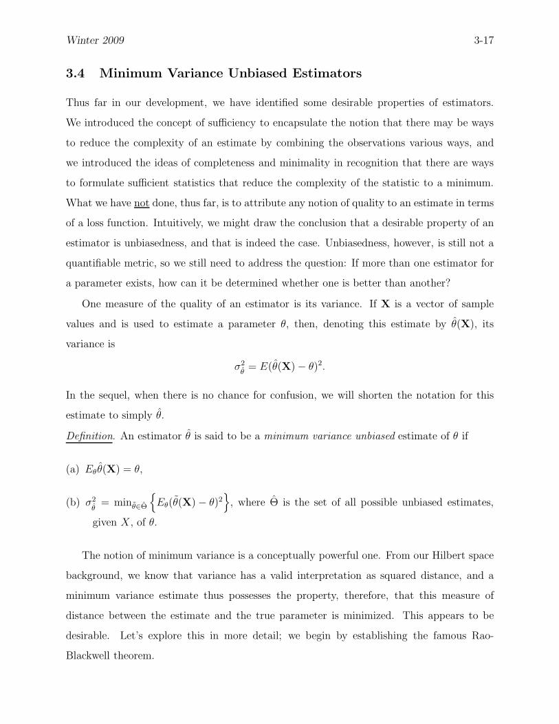
3.4 Minimum Variance Unbiased Estimators
Thus far in our development, we have identified some desirable properties of estimators.
We introduced the concept of sufficiency to encapsulate the notion that there may be ways
to reduce the complexity of an estimate by combining the observations various ways, and
we introduced the ideas of completeness and minimality in recognition that there are ways
to formulate sufficient statistics that reduce the complexity of the statistic to a minimum.
What we have not done, thus far, is to attribute any notion of quality to an estimate in terms
of a loss function. Intuitively, we might draw the conclusion that a desirable property of an
estimator is unbiasedness, and that is indeed the case. Unbiasedness, however, is still not a
quantifiable metric, so we still need to address the question: If more than one estimator for
a parameter exists, how can it be determined whether one is better than another?
One measure of the quality of an estimator is its variance. If X is a vector of sample
values and is used to estimate a parameter θ, then, denoting this estimate by θ(X), its
variance is
σ2θ
= E(θ(X) − θ)2.
In the sequel, when there is no chance for confusion, we will shorten the notation for this
estimate to simply θ.
Definition. An estimator θ is said to be a minimum variance unbiased estimate of θ if
(a) Eθ θ(X) = θ,
(b) σ2θ
= minθ∈Θ
Eθ(θ(X) − θ)2
, where Θ is the set of all possible unbiased estimates,
given X, of θ.
The notion of minimum variance is a conceptually powerful one. From our Hilbert space
background, we know that variance has a valid interpretation as squared distance, and a
minimum variance estimate thus possesses the property, therefore, that this measure of
distance between the estimate and the true parameter is minimized. This appears to be
desirable. Let’s explore this in more detail; we begin by establishing the famous Rao-
Blackwell theorem.

3-18 ECEn 672
Theorem 6 (Rao-Blackwell). Let Y be a random variable such that EθY = θ ∀θ ∈ Θ and
σ2Y = Eθ(Y − θ)2. Let Z be a random variable that is sufficient for θ, and let g(Z) be the
conditional expectation of Y given Z, i.e.,
g(Z) = E(Y |Z).
Then
(a) Eg(Z) = θ, and
(b) E(g(Z) − θ)2 ≤ σ2Y .
Proof.
The proof of (a) is immediate from Property 2 of conditional expectation:
Eg(Z) = E[E(Y |Z)] = EY = θ.
To establish (b), we write
σ2Y = E(Y − θ)2 = E[Y − g(Z) + g(Z) − θ]2
= E[Y − g(Z)]2︸ ︷︷ ︸
γ2
+ E[g(Z) − θ]2︸ ︷︷ ︸
σ2g(Z)
+2E[Y − g(Z)][g(Z)− θ]
We next examine the term E[Y − g(Z)][g(Z) − θ], and note that, by Properties 2 and 4 of
conditional expectations,
E[Y − g(Z)][g(Z)− θ] = E(E[Y − g(Z)] [g(Z) − θ]︸ ︷︷ ︸
function of Z
|Z)
= E([g(Z) − θ]E[Y − g(Z)] |Z)
= E([g(Z) − θ][EY − g(Z)︸ ︷︷ ︸
=0
] |Z) = 0.
Thus,
σ2Y = γ2 + σ2
g(Z),
which establishes (b). 2
The relevance of this theorem to us is as follows: Let X = X1, . . . , Xn be sample values
of a random variable X whose distribution is parameterized by θ ∈ Θ, and let Z = T (X)
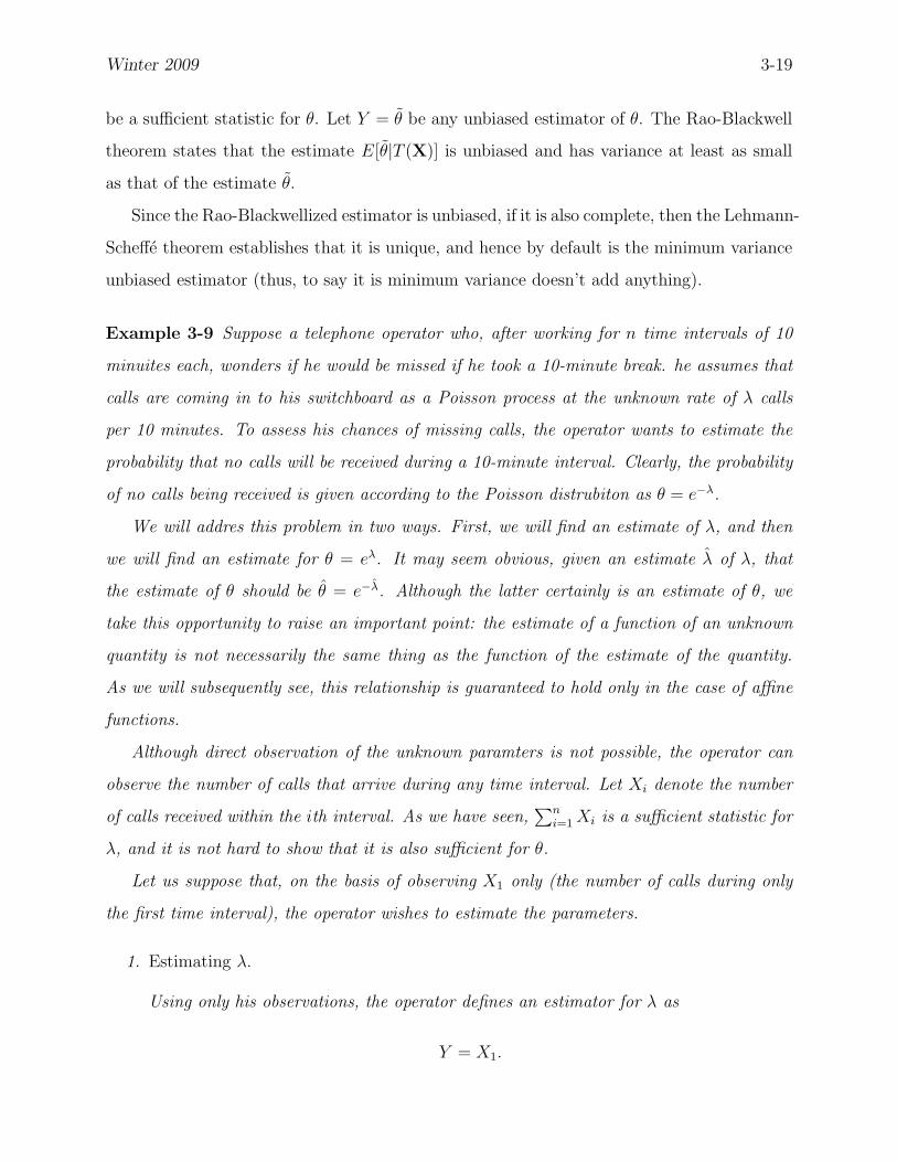
Winter 2009 3-19
be a sufficient statistic for θ. Let Y = θ be any unbiased estimator of θ. The Rao-Blackwell
theorem states that the estimate E[θ|T (X)] is unbiased and has variance at least as small
as that of the estimate θ.
Since the Rao-Blackwellized estimator is unbiased, if it is also complete, then the Lehmann-
Scheffe theorem establishes that it is unique, and hence by default is the minimum variance
unbiased estimator (thus, to say it is minimum variance doesn’t add anything).
Example 3-9 Suppose a telephone operator who, after working for n time intervals of 10
minuites each, wonders if he would be missed if he took a 10-minute break. he assumes that
calls are coming in to his switchboard as a Poisson process at the unknown rate of λ calls
per 10 minutes. To assess his chances of missing calls, the operator wants to estimate the
probability that no calls will be received during a 10-minute interval. Clearly, the probability
of no calls being received is given according to the Poisson distrubiton as θ = e−λ.
We will addres this problem in two ways. First, we will find an estimate of λ, and then
we will find an estimate for θ = eλ. It may seem obvious, given an estimate λ of λ, that
the estimate of θ should be θ = e−λ. Although the latter certainly is an estimate of θ, we
take this opportunity to raise an important point: the estimate of a function of an unknown
quantity is not necessarily the same thing as the function of the estimate of the quantity.
As we will subsequently see, this relationship is guaranteed to hold only in the case of affine
functions.
Although direct observation of the unknown paramters is not possible, the operator can
observe the number of calls that arrive during any time interval. Let Xi denote the number
of calls received within the ith interval. As we have seen,∑n
i=1 Xi is a sufficient statistic for
λ, and it is not hard to show that it is also sufficient for θ.
Let us suppose that, on the basis of observing X1 only (the number of calls during only
the first time interval), the operator wishes to estimate the parameters.
1. Estimating λ.
Using only his observations, the operator defines an estimator for λ as
Y = X1.
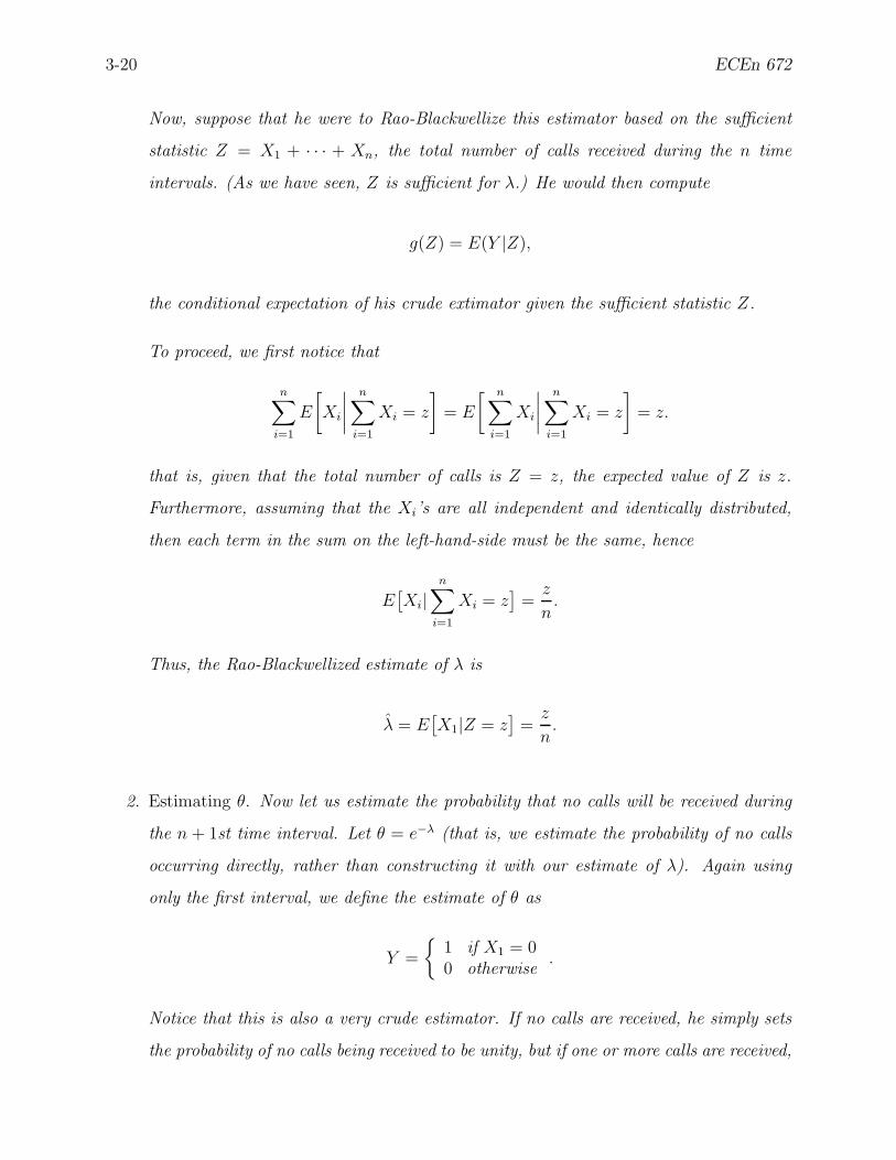
3-20 ECEn 672
Now, suppose that he were to Rao-Blackwellize this estimator based on the sufficient
statistic Z = X1 + · · · + Xn, the total number of calls received during the n time
intervals. (As we have seen, Z is sufficient for λ.) He would then compute
g(Z) = E(Y |Z),
the conditional expectation of his crude extimator given the sufficient statistic Z.
To proceed, we first notice that
n∑
i=1
E
[
Xi
∣∣∣∣
n∑
i=1
Xi = z
]
= E
[ n∑
i=1
Xi
∣∣∣∣
n∑
i=1
Xi = z
]
= z.
that is, given that the total number of calls is Z = z, the expected value of Z is z.
Furthermore, assuming that the Xi’s are all independent and identically distributed,
then each term in the sum on the left-hand-side must be the same, hence
E[Xi|
n∑
i=1
Xi = z]
=z
n.
Thus, the Rao-Blackwellized estimate of λ is
λ = E[X1|Z = z
]=
z
n.
2. Estimating θ. Now let us estimate the probability that no calls will be received during
the n + 1st time interval. Let θ = e−λ (that is, we estimate the probability of no calls
occurring directly, rather than constructing it with our estimate of λ). Again using
only the first interval, we define the estimate of θ as
Y =
1 if X1 = 00 otherwise
.
Notice that this is also a very crude estimator. If no calls are received, he simply sets
the probability of no calls being received to be unity, but if one or more calls are received,
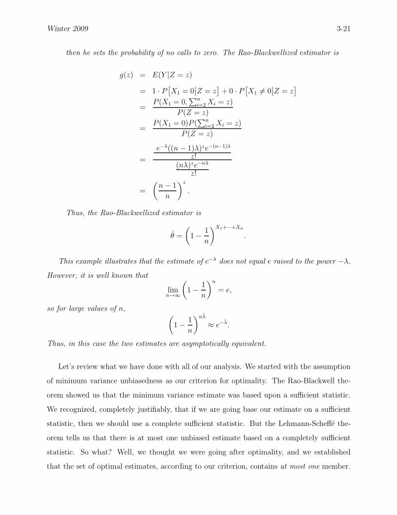
Winter 2009 3-21
then he sets the probability of no calls to zero. The Rao-Blackwellized estimator is
g(z) = E(Y |Z = z)
= 1 · P[X1 = 0
∣∣Z = z
]+ 0 · P
[X1 6= 0
∣∣Z = z
]
=P (X1 = 0,
∑ni=2 Xi = z)
P (Z = z)
=P (X1 = 0)P (
∑ni=2 Xi = z)
P (Z = z)
=
e−λ((n − 1)λ)ze−(n−1)λ
z!(nλ)ze−nλ
z!
=
(n − 1
n
)z
.
Thus, the Rao-Blackwellized estimator is
θ =
(
1 − 1
n
)X1+···+Xn
.
This example illustrates that the estimate of e−λ does not equal e raised to the power −λ.
However, it is well known that
limn→∞
(
1 − 1
n
)n
= e,
so for large values of n,(
1 − 1
n
)nλ
≈ e−λ.
Thus, in this case the two estimates are asymptotically equivalent.
Let’s review what we have done with all of our analysis. We started with the assumption
of minimum variance unbiasedness as our criterion for optimality. The Rao-Blackwell the-
orem showed us that the minimum variance estimate was based upon a sufficient statistic.
We recognized, completely justifiably, that if we are going base our estimate on a sufficient
statistic, then we should use a complete sufficient statistic. But the Lehmann-Scheffe the-
orem tells us that there is at most one unbiased estimate based on a completely sufficient
statistic. So what? Well, we thought we were going after optimality, and we established
that the set of optimal estimates, according to our criterion, contains at most one member.

3-22 ECEn 672
Thus, if you have found an unbiased estimate based on a complete sufficient statistic, not
only is it the best one, it is the only one. What we really have done is to establish one and
only one useful fact: The minimum variance unbiased estimate of a parameter is a function
of a complete sufficient statistic. Nothing more, nothing less.
Example 3-10 Let X = X1, . . . , Xn be a sample from the distribution N (µ, σ2). We know
that T1(X) =∑n
i=1 Xi and T2(X) =∑n
i=1 X2i are sufficient for (µ, σ2). By virtue of the fact
that the normal distribution is an exponential family, we have immediately that (T1, T2) are
also complete. Since 1nT1 and n−1
nT2 are unbiased estimates of µ and σ2, respectively, they
represent the minimum variance unbiased estimate of the mean and variance of the normally
distributed population random variable X.
Example 3-11 (From Ferguson) This example illustrates the dubious optimality of mini-
mum variance unbiasedness. Continuing with the telephone opertor, suppose that, working
for only 10 minutes, wonders if he would be missed if he took a 20-minute break. As before,
we assume that calls are coming in to his switchboard as a Poisson process at the unknown
rate of λ calls per 10 minutes. Let X denote the number of calls received within the first 10
minutes. As we have seen, X is a sufficient statistic for λ. On the basis of observing X, the
operator wishes to estimate the probability that no calls will be received within the next 20
minutes. Since the probability of no calls in any 10-minute interval is fX(0) = λ0
0!e−λ, the
probability of no calls in a 20-minute interval is θ = e−2λ. If the operator is enamored with
unbiased estimates, he will look for an estimate θ(X) for which
Eλθ(X) =∞∑
x=0
θ(x)e−λλx
x!≡ e−2λ.
After multiplying both sides by eλ and expanding e−λ in a power series, he would obtain
∞∑
x=0
θ(x)λx
x!≡
∞∑
x=0
(−1)x λx
x!.
Two convergent power series can be equal only if corresponding coefficients are equal. The
only unbiased estimate of θ = e−2λ is θ(x) = (−1)x. Thus he would estimate the probability
of receiving no calls in the next 20 minutes as +1 if he received an even number of calls in

Winter 2009 3-23
the last 10 minutes, and as −1 if he received an odd number of calls in the last 10 minutes.
This ridiculous estimate nonetheless a minimum-variance unbiased estimate.
At first glance the results of Examples 3-9 and 3-11 seem to be incongrous. On the one
hand, the estimate has an intuitively pleasing structure, while the other is patently redicu-
lous. Yet, both are claimed to be minimim-variance unbiased estimates of the probability of
no phone calls occurring. But it must be remembered that the two estimators use the data
differently. For the estimator given by Example 3-9, the estimator uses the actual number
of calls, while the estimator given in Example 3-11 uses only the odd/even properties of the
number of calls.
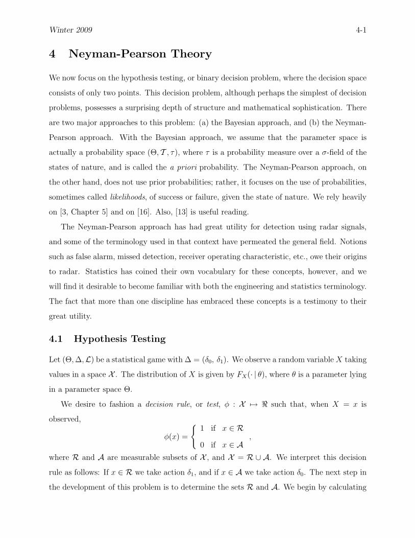
Winter 2009 4-1
4 Neyman-Pearson Theory
We now focus on the hypothesis testing, or binary decision problem, where the decision space
consists of only two points. This decision problem, although perhaps the simplest of decision
problems, possesses a surprising depth of structure and mathematical sophistication. There
are two major approaches to this problem: (a) the Bayesian approach, and (b) the Neyman-
Pearson approach. With the Bayesian approach, we assume that the parameter space is
actually a probability space (Θ, T , τ), where τ is a probability measure over a σ-field of the
states of nature, and is called the a priori probability. The Neyman-Pearson approach, on
the other hand, does not use prior probabilities; rather, it focuses on the use of probabilities,
sometimes called likelihoods, of success or failure, given the state of nature. We rely heavily
on [3, Chapter 5] and on [16]. Also, [13] is useful reading.
The Neyman-Pearson approach has had great utility for detection using radar signals,
and some of the terminology used in that context have permeated the general field. Notions
such as false alarm, missed detection, receiver operating characteristic, etc., owe their origins
to radar. Statistics has coined their own vocabulary for these concepts, however, and we
will find it desirable to become familiar with both the engineering and statistics terminology.
The fact that more than one discipline has embraced these concepts is a testimony to their
great utility.
4.1 Hypothesis Testing
Let (Θ, ∆,L) be a statistical game with ∆ = (δ0, δ1). We observe a random variable X taking
values in a space X . The distribution of X is given by FX(· | θ), where θ is a parameter lying
in a parameter space Θ.
We desire to fashion a decision rule, or test, φ : X 7→ < such that, when X = x is
observed,
φ(x) =
1 if x ∈ R
0 if x ∈ A,
where R and A are measurable subsets of X , and X = R ∪ A. We interpret this decision
rule as follows: If x ∈ R we take action δ1, and if x ∈ A we take action δ0. The next step in
the development of this problem is to determine the sets R and A. We begin by calculating

4-2 ECEn 672
the expectation of the decision rule. We observe that
Eθφ(X) = 1 · P (R| θ) + 0 · [1 − P (R| θ)]
= P (R| θ).
The expectation Eθφ(X) is called the power function corresponding to the decision rule (or
test) φ.
We will assume that Θ can be written Θ = Θ0 ∪ Θ1, for some disjoint sets Θ0 and Θ1,
and define the hypotheses H0 and H1 as
H0 : θ ∈ Θ0
H1 : θ ∈ Θ1
.
This classical decision problem gives rise to following terminology: H0 is called the null
hypothesis to mean that θ ∈ Θ0, and the alternative hypothesis to mean that θ ∈ Θ1. Only
one of these disjoint hypotheses is true, and our job is to guess which one. If we guess
correctly, the loss is zero, and if we guess incorrectly, the loss is one. The decision δ0 may
be considered as taking the action “accept H0,” and the decision δ1 the action “accept H1,”
or “reject H0.”
4.2 Simple Hypothesis versus Simple Alternative
We first look at the case where H0 and H1 are simple, that is, Θ0 and Θ1 each contain exactly
one element, Θ0 = θ0 and Θ1 = θ1. Then, if θ0 is the true value of the parameter, we
prefer to take action δ0, whereas if θ1 is the true value we prefer δ1.
Definition. The probability of rejecting the null hypothesis H0 when it is true is called the
size of the rule φ, and is denoted α. This is called a type I error, or false alarm. We thus
have
α = P [φ(X) = 1 | θ0]
= Eθ0φ(X)
= PFA,
where PFA is standard notion for the probability of a false alarm. This latter terminology
stems from radar applications, where a pulsed electromagnetic signal is transmitted. If a

Winter 2009 4-3
return signal is reflected from the target, we say a target is detected. But due to receiver
noise, atmospheric disturbances, spurious reflections from the ground and other objects, and
other signal distortions, it is not possible to determine with absolute certainty whether or
not a target is present.
Definition. The power, or detection probability, of a decision rule φ is the probability of
correctly accepting the alternative hypothesis, H1, when it is true, and is denoted by β. One
minus the power is the probability of accepting H0 when H1 is true, resulting in a type II
error, or missed detection. We thus have
β = P [φ(X) = 1 | θ1]
= Eθ1φ(X)
= PD,
where PD is standard notion for the probability of a detection, and
PMD = Eθ1 [1 − φ(X)]
is the probability of a missed detection.
Definition. A test φ is said to be best of size α for testing H0 against H1 if Eθ0φ(X) = α
and if for every test φ′ for which Eθ0φ′(X) ≤ α we have
β = Eθ1φ(X) ≥ Eθ1φ′(X) = β ′;
that is, a test φ is best of size α if, out of all tests with PFA not greater than α, φ has the
largest probability of detection, that is, it is the most powerful test.
4.3 The Neyman-Pearson Lemma
We now give a general method for finding the best tests of a simple hypothesis against a
simple alternative. This test is provided by the fundamental lemma of Neyman and Pearson.
Lemma 1 (Neyman-Pearson Lemma). Suppose that Θ = θ0, θ1 and that the distributions
of X have densities (or mass functions) fX(x | θ).
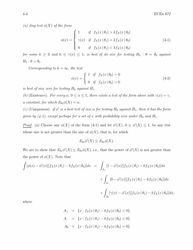
4-4 ECEn 672
(a) Any test φ(X) of the form
φ(x) =
1 if fX(x | θ1) > kfX(x | θ0)
γ(x) if fX(x | θ1) = kfX(x | θ0)
0 if fX(x | θ1) < kfX(x | θ0)
(4-1)
for some k ≥ 0 and 0 ≤ γ(x) ≤ 1, is best of its size for testing H0 : θ = θ0 against
H1 : θ = θ1.
Corresponding to k = ∞, the test
φ(x) =
1 if fX(x | θ0) = 0
0 if fX(x | θ0) > 0(4-2)
is best of size zero for testing H0 against H1.
(b) (Existence). For every α, 0 ≤ α ≤ 1, there exists a test of the form above with γ(x) = γ,
a constant, for which Eθ0φ(X) = α.
(c) (Uniqueness). if φ′ is a best test of size α for testing H0 against H1, then it has the form
given by (4-1), except perhaps for a set of x with probability zero under H0 and H1.
Proof. (a) Choose any φ(X) of the form (4-1) and let φ′(X), 0 ≤ φ′(X) ≤ 1, be any test
whose size is not greater than the size of φ(X), that is, for which
Eθ0φ′(X) ≤ Eθ0φ(X).
We are to show that Eθ1φ′(X) ≤ Eθ1φ(X), i.e., that the power of φ′(X) is not greater than
the power of φ(X). Note that∫
[φ(x) − φ′(x)][fX(x | θ1) − kfX(x | θ0)]dx =
∫
A+
[1 − φ′(x)][fX(x | θ1) − kfX(x | θ0)]dx
+
∫
A−
[0 − φ′(x)][fX(x | θ1) − kfX(x | θ0)]dx
+
∫
A0
[γ(x) − φ′(x)][fX(x | θ1) − kfX(x | θ0)]dx,
where
A+ = x : fX(x | θ1) − kfX(x | θ0) > 0
A− = x : fX(x | θ1) − kfX(x | θ0) < 0
A0 = x : fX(x | θ1) − kfX(x | θ0) = 0

Winter 2009 4-5
Since φ′(x) ≤ 1, the first integral is nonnegative. Also, the second integral is nonnegative
by inspection, and the third integral is identically zero. Thus,
∫
[φ(x) − φ′(x)][fX(x | θ1) − kfX(x | θ0)]dx ≥ 0. (4-3)
This implies that
Eθ1φ(X) − Eθ1φ′(X) ≥ kEθ0φ(X) − kEθ0φ
′(X) ≥ 0,
where the last inequality is a consequence of the hypothesis that Eθ0φ′(X) ≤ Eθ0φ(X). This
proves that φ(X) is more powerful than φ′(X), i.e.,
β − β ′ ≥ k(α − α′).
For the case k = ∞, any test φ′ of size α = 0 must satisfy
α =
∫
φ′(x)fX(x | θ0)dx = 0, (4-4)
hence φ′(x) must be zero almost everywhere on the set x : fX(x, | θ0) > 0. Thus, using
this result and (4-2),
Eθ1 [φ(X) − φ′(X)] =
∫
x:fX(x|θ0)>0(φ(x) − φ′(x))fX(x | θ1)dx
︸ ︷︷ ︸
=0
+
∫
x:fX(x|θ0)=0(φ(x) − φ′(x))fX(x | θ1)dx
=
∫
x:fX(x|θ0)=0(1 − φ′(x))fX(x | θ1)dx ≥ 0,
since φ(x) = 1 whenever the density fX(x | θ0) = 0 by (4-2), and φ′(x) ≤ 1. This completes
the proof of (a).
(b) Since a best test of size α = 0 is given by (4-2), we may restrict attention to 0 < α ≤ 1.
The size of the test (4-1), when γ(x) = γ, is
Eθ0φ(X) = Pθ0[fX(X | θ1) > kfX(X | θ0)] + γPθ0[fX(X | θ1) = kfX(X | θ0)]
= 1 − Pθ0 [fX(X | θ1) ≤ kfX(X | θ0)] + γPθ0[fX(X | θ1) = kfX(X | θ0)]. (4-5)

4-6 ECEn 672
For fixed α, 0 < α ≤ 1, we are to find k and γ so that Eθ0φ(X) = α, or equivalently using
the representation (4-5),
1 − Pθ0[fX(X | θ1) ≤ kfX(X | θ0)] + γPθ0 [fX(X | θ1) = kfX(X | θ0)] = α
or
Pθ0[fX(X | θ1) ≤ kfX(X | θ0)] − γPθ0[fX(X | θ1) = kfX(X | θ0)] = 1 − α. (4-6)
If there exists a k0 for which Pθ0[fX(X | θ1) ≤ kfX(X | θ0)] = 1 − α, we take γ = 0 and
k = k0. If not, then there is a discontinuity in Pθ0 [fX(X | θ1) ≤ kfX(X | θ0)] when viewed as
a function of k that brackets the particular value 1 − α, that is, there exists a k0 such that
Pθ0 [fX(X | θ1) < k0fX(X | θ0)] < 1 − α ≤ Pθ0 [fX(X | θ1) ≤ k0fX(X | θ0)]. (4-7)
Figure 4-1 illustrates this situation. Using (4-6) for 1 − α in (4-7) and solving the equation
1 − α ≤ Pθ0 [fX(X | θ1) ≤ k0fX(X | θ0)]
for γ yields
γ =Pθ0 [fX(X | θ1) ≤ k0fX(X | θ0)] − (1 − α)
Pθ0[fX(X | θ1) = k0fX(X | θ0)]
satisfies (4-6) and 0 ≤ γ ≤ 1, so letting k = k0, (b) is proved.
kk0
1
1 − α
Pθ0 [fX(X|θ1) ≤ kfX(X|θ0)]
Figure 4-1: Illustration of threshold for Neyman-Pearson test
(c) If α = 0, the argument in (a) shows that φ(x) = 0 almost everywhere on the set x :
fθ0(x) > 0. If φ′ has a minimum probability of the second kind of error, then 1− φ′(x) = 0

Winter 2009 4-7
almost everywhere on the set x : fθ1(x) > 0 ∼ x : fθ0(x) > 0. Thus φ′ differs from the
φ of (4-2) by a set of probability zero under either hypothesis.
If α > 0, let φ be the best test of size α of the form (4-1). Then, because Eθiφ(X) =
Eθiφ′(X), i = 0, 1, the integral (4-3) must be equal to zero. But because this integral
is nonnegative it must be zero almost everywhere; that is to say, on the set for which
fX(x | θ1) 6= fX(x | θ0) we have φ(x) = φ′(x) almost everywhere. Thus, except for a set of
probability zero, φ′(x) has the same form as (4-1) with the same value for k as φ(x), thus
the function φ(x) satisfies the uniqueness requirement. 2
The Neyman-Pearson lemma thus gives is a general decision rule for a simple hypothesis
versus a simple alternative. We would apply it as follows:
1. For a given binary decision problem, determine which hypothesis is to be the null, and
which is to be the alternative. This choice is at the discretion of the analyst. As a
practical issue, it would be wise to choose as the null hypothesis the one that has the
most serious consequences if rejected, because the analyst is able to choose the size of
the test, which enables control of probability of rejecting the null hypothesis when it
is true.
2. Select the size of the test. It seems to be the tradition for many applications to set
α = 0.05 or α = 0.01, which correspond to common “significance levels” used in
statistics. The main issue, however, is to choose the size relevant to the problem at
hand. For example, in a radar target detection problem, if the null hypothesis is “no
target present,” setting α = 0.05 means that we are willing to accept a 5% chance that
a target will not be there when our test tell us that a target is present. The smaller
the size, in general, the smaller also is the power, as will be made more evident in the
discussion of the receiver operator characteristic.
3. Calculate the threshold, k. The way to do this is not obvious from the theorem.
Clearly, k must be a function of the size, α, but until specific distributions are used,
there is no obvious formula for determining k. That will be one of the tasks examined
in the examples to follow.

4-8 ECEn 672
4.4 The Likelihood Ratio
The key quantities in the Neyman-Pearson theory are the density functions fX(x | θ1) and
fX(x | θ0). These quantities are sometimes viewed as the conditional pdf’s (or pmf’s) of X
given θ. The concept of conditioning, however, requires that the quantity θ be a random
variable. But nothing in the Neyman-Pearson theory requires θ to be so viewed; in fact, the
Neyman-Pearson approach is often considered to be an alternative to the Bayesian approach,
where θ is viewed as a random variable. Since the purists insist that the Neyman-Pearson
not be confused with the Bayesian approach, they have coined the term likelihood function
for fX(x | θ1) and fX(x | θ0). To keep with tradition and to keep any rabid anti-Bayesians in
the crowd from getting too overworked, we will respect this convention and call these things
likelihood functions, or likelihoods, when required (or when we think about it–engineers
don’t usually get too worked up over these types of issues, but perhaps they should).
The inequality fX(x | θ1)> = <kfX(x | θ0) has emerged as a natural expression in the
statement and proof of the Neyman-Pearson lemma. This inequality may be expressed as a
ratio:
`(x) =fX(x | θ1)
fX(x | θ0)> = <k.
The quantity `(x) is called the likelihood ratio, and the test (4-1) may be rewritten
φ(x) =
1 if `(x) > k
γ if `(x) = k
0 if `(x) < k
. (4-8)
You may have noticed in the proof of the lemma that we have used expressions such
as fX(X | θ1), where we have used the random variable X as an argument of the density
function. When we do this, the function fX(X | θ1) is, of course, a random variable since it
becomes a function of a random variable. The likelihood ratio `(X) = fX(X | θ1)fX(X | θ0)
then is also
a random variable.
A false alarm occurs (accepting H1 when H0 is true) if `(x) > k when θ = θ0 and X = x.
Let f`(l | θ0) denote the density of ` given θ = θ0; then
α = PFA = Pθ0 [`(X) > k] =
∫ ∞
k
f`(l, | θ0)dl,
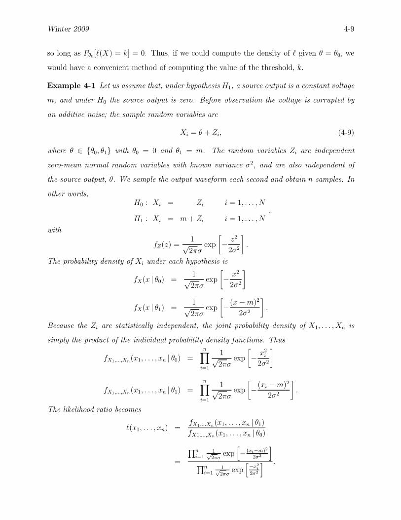
Winter 2009 4-9
so long as Pθ0 [`(X) = k] = 0. Thus, if we could compute the density of ` given θ = θ0, we
would have a convenient method of computing the value of the threshold, k.
Example 4-1 Let us assume that, under hypothesis H1, a source output is a constant voltage
m, and under H0 the source output is zero. Before observation the voltage is corrupted by
an additive noise; the sample random variables are
Xi = θ + Zi, (4-9)
where θ ∈ θ0, θ1 with θ0 = 0 and θ1 = m. The random variables Zi are independent
zero-mean normal random variables with known variance σ2, and are also independent of
the source output, θ. We sample the output waveform each second and obtain n samples. In
other words,H0 : Xi = Zi i = 1, . . . , N
H1 : Xi = m + Zi i = 1, . . . , N,
with
fZ(z) =1√2πσ
exp
[
− z2
2σ2
]
.
The probability density of Xi under each hypothesis is
fX(x | θ0) =1√2πσ
exp
[
− x2
2σ2
]
fX(x | θ1) =1√2πσ
exp
[
−(x − m)2
2σ2
]
.
Because the Zi are statistically independent, the joint probability density of X1, . . . , Xn is
simply the product of the individual probability density functions. Thus
fX1,...,Xn(x1, . . . , xn | θ0) =
n∏
i=1
1√2πσ
exp
[
− x2i
2σ2
]
fX1,...,Xn(x1, . . . , xn | θ1) =
n∏
i=1
1√2πσ
exp
[
−(xi − m)2
2σ2
]
.
The likelihood ratio becomes
`(x1, . . . , xn) =fX1,...Xn(x1, . . . , xn | θ1)
fX1,...,Xn(x1, . . . , xn | θ0)
=
∏ni=1
1√2πσ
exp[
− (xi−m)2
2σ2
]
∏ni=1
1√2πσ
exp[−x2
i
2σ2
] .

4-10 ECEn 672
After canceling common terms and taking the logarithm7, we have
log `(x1, . . . , xn) =m
σ2
n∑
i=1
xi −nm2
2σ2, (4-10)
resulting in the log likelihood ratio. It is interesting to see, in this example, that the only
data that appear in the likelihood ratio is through the sum∑n
i=1 xi, which is consistent with
our knowledge that∑n
i=1 Xi, is a sufficient statistic for the mean.
The log likelihood ratio test then becomes
φ(x1, . . . , xn) =
1 if log `(x1, . . . , xn) > log ν
γ if `(x1, . . . , xn) = ν
0 if log `(x1, . . . , xn) < log ν
, (4-11)
where ν is the threshold we need to calculate. Viewing the log likelihood ratio as a random
variable and multiplying (4-10) by σ/√
nm yields
σ√nm
log `(X1, . . . , Xn) =1√nσ
n∑
i=1
Xi −√
nm
2σ.
Define the new random variable
L(X1, . . . , Xn) =σ√nm
log `(X1, . . . , Xn) +
√nm
2σ
=1√nσ
n∑
i=1
Xi.
Under hypothesis H0, L is obtained by adding n independent zero-mean normal random
variables with variance σ2 and then dividing by√
nσ, yielding L ∼ N (0, 1), and under
hypothesis H1, L ∼ N (√
nm/σ, 1). Thus, for this example, we are able to calculate the
densities of the log likelihood ratio. The test becomes
φ(x1, . . . , xn) =
1 if L(x1, . . . , xn) > 1
dlog ν + d
2
0 if L(x1, . . . , xn) ≤ 1dlog ν + d
2
, (4-12)
where d =
√nmσ . Note, in (4-12) that we have set γ = 0 without loss of generality, since
Pθ[L(X1, . . . , Xn) = γ] = 0.
7We know we can do this without disturbing the structure of the test, since the logarithm is a monotonicfunction.

Winter 2009 4-11
The size, PFA, is the integral of the density fL(l | θ0) over the interval (1dlog ν + d
2, ∞),
or
PFA =
∫ ∞
1d
log ν+ d2
fL(l, | θ0)dl
=
∫ ∞
1d
log ν+ d2
1√2π
exp
[−l2
2
]
dl
= 1 − Φ
(log ν + d2/2
d
)
,
where
Φ(z) =
∫ z
−∞(2π)−
12 exp[−x2/2]dx
is the normal integral, corresponding to the area under the normal curve from −∞ to the
point z. Thus, to compute the threshold ν for a given size α, we solve (using normal tables
or a computer) 1 − Φ(z) = α for z, that is, compute z∗ = Φ−1(1 − α), then calculate
ν = z∗d − d2
2.
Similarly, the power, PD, is the integral of the density fL(l | θ1) over the interval (1dlog ν+
d2, ∞), or
PD =
∫ ∞
1d
log ν+ d2
fL(l, | θ1)dl
=
∫ ∞
1d
log ν+ d2
1√2π
exp
[−(l − d)2
2
]
dl
=
∫ ∞
1d
log ν− d2
1√2π
exp
[−y2
2
]
dy
= 1 − Φ
(log ν − d2/2
d
)
.
Figure 4-2 illustrates the normal curves for the two hypotheses under question, and the
regions corresponding to PFA and PD are indicated in the figure.
4.5 Receiver Operating Characteristic
For a Neyman-Pearson test, the size and power, as specified by PFA and PD, completely
specify the test performance. We can gain some valuable insight by cross-plotting these
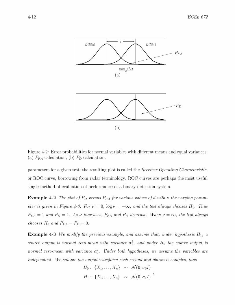
4-12 ECEn 672
(a)
(b)
f`(l|θ0) f`(l|θ1)d -
log η−d2/2d
9
PFA
9
PD
Figure 4-2: Error probabilities for normal variables with different means and equal variances:(a) PFA calculation, (b) PD calculation.
parameters for a given test; the resulting plot is called the Receiver Operating Characteristic,
or ROC curve, borrowing from radar terminology. ROC curves are perhaps the most useful
single method of evaluation of performance of a binary detection system.
Example 4-2 The plot of PD versus PFA for various values of d with ν the varying param-
eter is given in Figure 4-3. For ν = 0, log ν = −∞, and the test always chooses H1. Thus
PFA = 1 and PD = 1. As ν increases, PFA and PD decrease. When ν = ∞, the test always
chooses H0 and PFA = PD = 0.
Example 4-3 We modify the previous example, and assume that, under hypothesis H1, a
source output is normal zero-mean with variance σ21, and under H0 the source output is
normal zero-mean with variance σ20. Under both hypotheses, we assume the variables are
independent. We sample the output waveform each second and obtain n samples, thus
H0 : X1, . . . , Xn ∼ N (0, σ0I)
H1 : Xi, . . . , Xn ∼ N (0, σ1I),

Winter 2009 4-13
0 0.2 0.4 0.6 0.8 1
0
0.2
0.4
0.6
0.8
1
PFA →
PD
↑
d=1
d=2
d=3
increasing ν
Figure 4-3: Receiver operating characteristic: normal variables with unequal means andequal variances.
that is, with Θ = θ0, θ1 = σ20 , σ2
1,
fX1,...,Xn(x1, . . . , xn | θ0) =n∏
i=1
1√2πσ0
exp
[
− x2i
2σ20
]
fX1,...,Xn(x1, . . . , xn | θ1) =
n∏
i=1
1√2πσ1
exp
[
− x2i
2σ21
]
.
The likelihood ratio becomes
`(x1, . . . , xn) =fX1,...Xn(x1, . . . , xn | θ1)
fX1,...,Xn(x1, . . . , xn | θ0)
=
∏ni=1
1√2πσ1
exp[
− x2i
2σ21
]
∏ni=1
1√2πσ0
exp[
− x2i
2σ20
] .
After canceling common terms and taking the logarithm, we have
log `(x1, . . . , xn) =1
2
(1
σ21
− 1
σ20
) n∑
i=1
x2i + n log
σ0
σ1
. (4-13)
The log likelihood ratio test then becomes
φ(x1, . . . , xn) =
1 if log `(x, . . . , xn) > log ν
γ if `(x1, . . . , xn) = ν
0 if log `(x1, . . . , xn) < log ν
, (4-14)

4-14 ECEn 672
where ν is the threshold. Assume σ21 > σ2
0, and define the new random variable
L(X1, . . . , Xn) =2σ2
0σ21
σ21 − σ2
0
(
log `(X1, . . . , Xn) − n logσ0
σ1
)
.
We may then replace the test (4-14) by the test
φ(x1, . . . , xn) =
1 if L(x1, . . . , xn) > ε
0 if L(x1, . . . , xn) < ε, (4-15)
where
ε =2σ2
0σ21
σ21 − σ2
0
(
log ν − n logσ0
σ1
)
.
This problem is slightly more involved than the previous example, since the random vari-
able `(X), given θ, is not normally distributed. We can simplify things a lot, however, if we
deal with the special case n = 2. Then
PFA = Pθ0(L ≥ ε) = Pθ0(X21 + X2
2 ≥ ε).
To evaluate the expression on the right, we change to polar coordinates:
x1 = u cos v, u =√
x21 + x2
2
x2 = u sin v, v = tan−1 x1
x2
.
Then
Pθ0(U2 ≥ ε) =
∫ 2π
0
∫ ∞
√ε
u1
2πσ20
exp
(
− u2
2σ20
)
dudv.
Integrating with respect to v, we have
PFA =
∫ ∞
√ε
u1
σ20
exp
(
− u2
2σ20
)
du.
Since L = U2, changing variables l = u2 yields
PFA =
∫ ∞
ε
1
σ20
exp
(
− l
2σ20
)
dl = exp
(
− ε
2σ20
)
.
Similarly,
PD = exp
(
− ε
2σ21
)
.

Winter 2009 4-15
The threshold for (4-15) is then
ε = −2σ20 log PFA.
We observe that the threshold does not depend upon σ21; the power of the test, however, does
depend on this quantity. To construct the ROC we combine these expressions, eliminate γ,
and obtain
PD = (PFA)σ20/σ2
1 ,
or in terms of logarithms,
log PD =σ2
0
σ21
log PFA.
As expected, the performance improves monotonically as the ratio r =σ21
σ20
increases. Figure
4-4 illustrates this case.
0 0.2 0.4 0.6 0.8 1
0
0.2
0.4
0.6
0.8
1
PFA →
PD
↑
r=4
r=3
r=2
r=1
Figure 4-4: Receiver operating characteristic: normal variables with equal means and un-equal variances.
We now develop some important properties of the ROC.
Property 1 All continuous likelihood ratio tests have ROC curves that are concave down-
ward.
Proof. Suppose the ROC has a segment that is convex. To be specific, suppose
(P aFA, P a
D) and (P bFA, P b
d ) are points on the ROC curve, but the curve is convex between
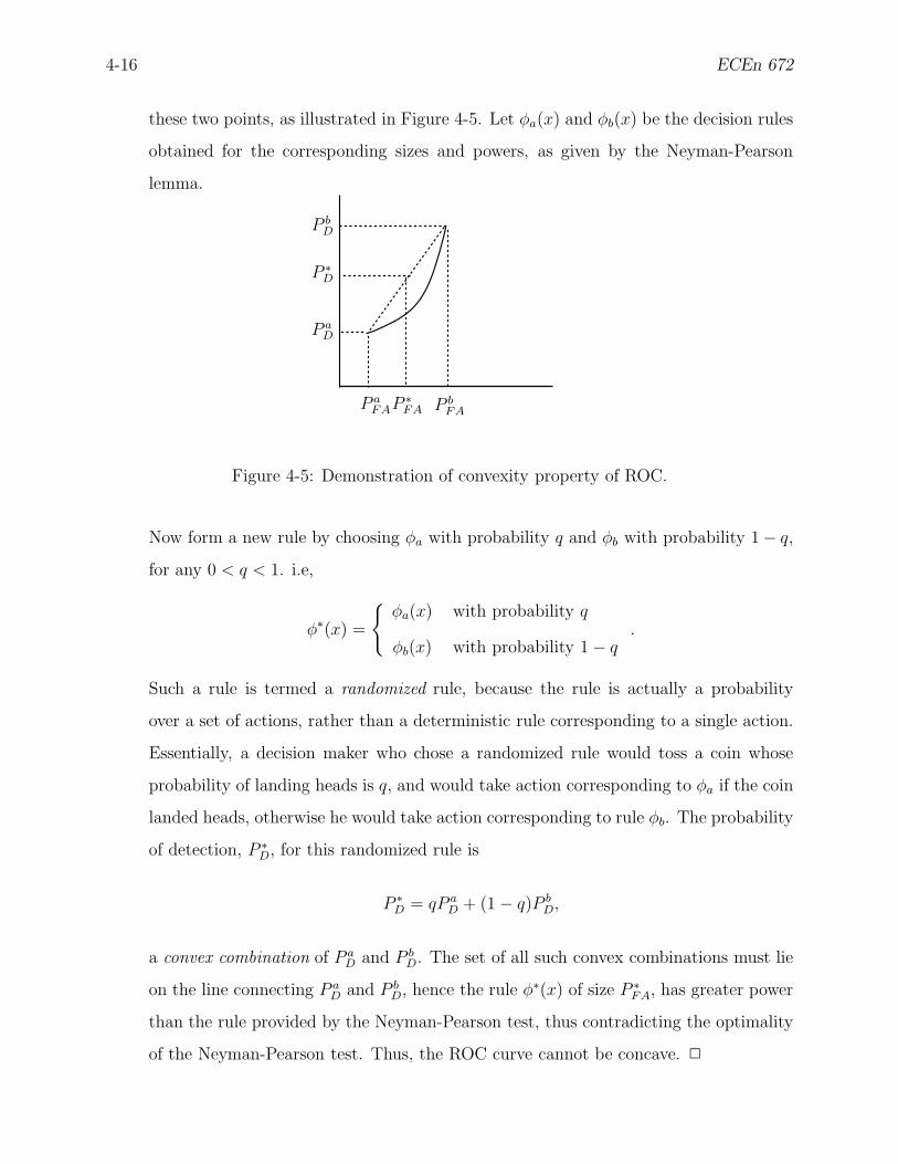
4-16 ECEn 672
these two points, as illustrated in Figure 4-5. Let φa(x) and φb(x) be the decision rules
obtained for the corresponding sizes and powers, as given by the Neyman-Pearson
lemma.
P aFA P b
FAP ∗FA
P aD
P ∗D
P bD
Figure 4-5: Demonstration of convexity property of ROC.
Now form a new rule by choosing φa with probability q and φb with probability 1− q,
for any 0 < q < 1. i.e,
φ∗(x) =
φa(x) with probability q
φb(x) with probability 1 − q.
Such a rule is termed a randomized rule, because the rule is actually a probability
over a set of actions, rather than a deterministic rule corresponding to a single action.
Essentially, a decision maker who chose a randomized rule would toss a coin whose
probability of landing heads is q, and would take action corresponding to φa if the coin
landed heads, otherwise he would take action corresponding to rule φb. The probability
of detection, P ∗D, for this randomized rule is
P ∗D = qP a
D + (1 − q)P bD,
a convex combination of P aD and P b
D. The set of all such convex combinations must lie
on the line connecting P aD and P b
D, hence the rule φ∗(x) of size P ∗FA, has greater power
than the rule provided by the Neyman-Pearson test, thus contradicting the optimality
of the Neyman-Pearson test. Thus, the ROC curve cannot be concave. 2

Winter 2009 4-17
Property 2 All continuous likelihood ratio tests have ROC curves that are above the PD =
PFA line. This is just a special case of Property 1 because the points (0, 0) and (1, 1)
are contained on all ROC curves.
Property 3 The slope of the ROC curve at a particular point is equal to the value of the
threshold k required to achieve the PD and PFA of that point.
Proof. Let ` be the likelihood ratio, and suppose k is a given threshold. Then
PD =
∫ ∞
k
f`(l | θ1)dl
PFA =
∫ ∞
k
f`(l | θ0)dl.
Let δ be a small perturbation in the threshold; then
∆PD =
∫ k+δ
k
f`(l | θ1)dl
∆PFA =
∫ k+δ
k
f`(l | θ0)dl
represent the changes in PD and PFA, respectively, as a result of the change in threshold.
Then the slope of the ROC curve is given by
limδ→0
∆PD
∆PFA= lim
δ→0
δf`(k | θ1)
δf`(k | θ0)=
f`(k | θ1)
f`(k | θ0). (4-16)
To establish that this ratio equals k, we we observe that, in general,
Eθ1`n(X) =
∫
`n(x)fX(x | θ1)dx
=
∫fn
X(x | θ1)
fnX(x | θ0)
fX(x | θ1)dx
=
∫fn+1
X (x | θ1)
fn+1X (x | θ0)
fX(x | θ0)dx
=
∫
`n+1(X)fX(x | θ1)dx
= Eθ0`n+1(X).
4-18 ECEn 672
But the condition Eθ1`n = Eθ0`
n+1 requires that
∫
lnf`(l | θ1)dl =
∫
ln+1f`(l | θ0)dl
must hold for all n, which implies that
f`(l | θ1) = lf`(l | θ0) (4-17)
must hold for all values of l. Thus, applying (4-17) to (4-16), we obtain the desired
result:dPD
dPFA=
f`(k | θ1)
f`(k | θ0)= k.
2
4.6 Composite Binary Hypotheses
Thus far, we have dealt with the simplest form of binary hypothesis testing: a simple hypoth-
esis versus a simple alternative. We now generalize our thinking to composite hypotheses.
Definition. A hypothesis H : θ ∈ Θ0 is said to be composite if Θ0 consists of at least two
elements.
We are interested in testing a composite hypothesis H0 : θ ∈ Θ0 against a composite alter-
native H1 : θ ∈ Θ1. Before pursuing the development of a theory for composite hypotheses,
we need to generalize the notions of size and power for this situation.
Definition. A test φ of H0 : θ ∈ Θ0 against H1 : θ ∈ Θ1 is said to have size α if
supθ∈Θ0
Eθφ(X) = α.
Definition. A test φ0 is said to be uniformly most powerful (UMP) of size α for testing
H0 : θ ∈ Θ0 against H1 : θ ∈ Θ1 if φ0 is of size α and if, for any other test φ of size at most
α,
Eθφ0(X) ≥ Eθφ(X)
for each θ ∈ Θ1.
For a test to be UMP, it must maximize the power Eθφ(X) for each θ ∈ Θ1. This is a very
stringent condition, and the existence of a uniformly most powerful test is not guaranteed

Winter 2009 4-19
in all cases. For example, although the Neyman-Pearson lemma tells us that there exists a
most powerful test of size α for fixed θ1 ∈ Θ1, there is no reason why this same test should
also be most powerful of size α for θ2 6= θ1, with θ2 ∈ Θ1. Our goal in this section is to
arrive at conditions for which the existence of a UMP can indeed be guaranteed. That is, we
want to establish conditions under which there exists a test such that the probability of false
alarm is less than a given α for all θ ∈ Θ0, but at the same time has maximum probability
of detection for all θ ∈ Θ1.
We will approach this development through an example; this result will motivate the
characterization of the conditions for the existence of a UMP test.
Illustrative Example. Let X be a unit-variance normal random variable and unknown mean
θ. Let Θ0 = (−∞, θ0], and let Θ1 = (θ0,∞). We wish to test H0 : θ ∈ Θ0 against H1 : θ ∈ Θ1.
We desire the test to be uniformly most powerful out of the class of all tests φ for which
Eθφ(X) ≤ α ∀θ ≤ θ0. (4-18)
To solve this problem we first solve a related problem, and seek the best test φ0 of size
α for testing the simple hypothesis H ′0 : θ = θ0 against the simple alternative H ′
1 : θ = θ1,
where θ1 > θ0. By the Neyman-Pearson lemma, this test is of the form
φ0(x) =
1 if 1√2π
exp[−(x − θ1)2/2] > k√
2πexp[−(x − θ0)
2/2]
γ if 1√2π
exp[−(x − θ1)2/2] = k√
2πexp[−(x − θ0)
2/2]
0 if 1√2π
exp[−(x − θ1)2/2] < k√
2πexp[−(x − θ0)
2/2]
.
After taking logarithms and rearranging, this test assumes an equivalent form
φ0(x) =
1 if x > k′
0 if otherwise, (4-19)
where
k′ =(θ2
1/2 − θ20/2) + log k
(θ1 − θ0).
Note that we may set γ = 0 since the probability that X = k′ is zero. With this test, we see
4-20 ECEn 672
that
Pθ0 [X > k′] =
∫ ∞
k′
1√2π
exp[−(x − θ0)2/2]dx
=
∫ ∞
k′−θ0
1√2π
exp[−x2/2]dx
= α
implies that k′ − θ0 = Φ−1(1 − α), or
k′ = θ0 + Φ−1(1 − α). (4-20)
It is important to note that k′ depends only on θ0 and α, but not otherwise on θ1. In fact,
exactly the same test as given by (4-19), with k′ determined by (4-20), is best, according to
the Neyman-Pearson lemma for all θ1 ∈ (θ0, ∞). Thus, φ0 given by (4-19) is UMP out of
the class of all tests for which
Eθ0φ(X) ≤ α.
We have thus established that φ0 is UMP for H0 : θ = θ0 (simple) and H1 : θ > θ0
(composite). To complete the development, we need to extend the discussion to permit
H0 : θ ≤ θ0 (composite). We may do this by establishing that φ0 satisfies the condition given
by (4-18). Fix k′ by (4-20) for the given α. Now examine
Eθφ0(X) = Pθ[X > k′]
=
∫ ∞
k′
1√2π
exp[−(x − θ)2/2]dx,
and note that this quantity is an increasing function of θ (k′ being fixed). Hence,
Eθφ0(X) < Eθ0φ0(X) ≤ α ∀θ ≤ θ0
and, consequently,
supθ∈(−∞, θ0]
Eθφ0(X) ≤ α.
Hence, φ0 is uniformly best out of all tests satisfying (4-18), i.e., it is UMP.
Summarizing, we have established that there does indeed exist a uniformly most powerful
test for testing the hypothesis H0 : θ ≤ θ0 against the alternatives H1 : θ > θ0, for any θ0
Winter 2009 4-21
where θ0 is the mean of a normal random variable X with known variance. Such a test is
said to be one-sided, and has very simple form: reject H0 if X > k′ and accept H0 if X ≤ k′,
where k′ is chosen to make the size of the test equal to α.
We now turn attention to the issue of determining what conditions on the distribution
are sufficient to guarantee the existence of a UMP.
Definition. A real parameter family of distributions is said to have monotone likelihood ratio
if densities (or probability mass functions) f(x | θ) exist such that, whenever θ1 < θ2, the
likelihood ratio
`(x) =f(x | θ2)
f(x | θ1)
is a nondecreasing function of x in the set of its existence; that is, for x in the set of points
for which at least one of f(x | θ1) and f(x | θ2) is positive. If f(x | θ1) = 0 and f(x | θ2) > 0,
the likelihood ratio is defined as +∞. Thus, if the distribution has monotone likelihood
ratio, the larger x the more likely the alternative, H1, is to be true.
Theorem 1 (Karlin and Rubin). If the distribution of X has monotone likelihood ratio,
then any test of the form
φ(x) =
1 if x > x0
γ if x = x0
0 if x < x0
(4-21)
has nondecreasing power. Any test of the form (4-21) is UMP of its size for testing H0 : θ ≤θ0 against H1 : θ > θ0 for any θ0 ∈ Θ, provided its size is not zero. For every 0 < α ≤ 1 and
every θ0 ∈ Θ, there exist numbers −∞ < x0 < ∞ and 0 ≤ γ ≤ 1 such that the test (4-21) is
UMP of size α for testing H0 : θ ≤ θ0 against H1 : θ > θ0.
Proof. Let θ1 and θ2 be any points of Θ with θ1 < θ2. By the Neyman-Pearson lemma, any
test of the form
φ(x) =
1 if fX(x | θ2) > kfX(x | θ1)
γ if fX(x | θ2) = kfX(x | θ1)
0 if fX(x | θ2) < kfX(x | θ1)
(4-22)
for 0 ≤ k < ∞, is best of its size for testing θ = θ1 against θ = θ2. Because the distribution
has monotone likelihood ratio, any test of the form (4-21) is also of the form (4-22). To see

4-22 ECEn 672
this, note that if x′ < x0, then `(x′) ≤ `(x0). For any k in the range of ` there exists a x0
such that if `(x) = k, then x = x0. Thus, (4-21) is best of size α > 0 for testing θ = θ1
against θ = θ2. The remainder of the proof is essentially the same as the proof for the normal
distribution, and will be omitted. 2
Example 4-4 The one-parameter exponential family of distributions with density (or prob-
ability mass function)
f(x | θ) = c(θ)h(x) exp[π(θ)t(x)]
has a monotone likelihood ratio provided that both π and t are nondecreasing. To see this,
simply write, with θ1 < θ2,
f(x | θ2)
f(x | θ1)=
c(θ2)
c(θ1)exp [π(θ2) − π(θ1)]t(x) ,
which is nondecreasing in x.

Winter 2009 5-1
5 Bayes Decision Theory
Thus far, our treatment of decision theory has been to consider the parameter as an unknown
quantity, but not a random variable, and formulate a decision rule on the basis of maximizing
the probability of correct detection (the power) while at the same time attempting to keep
the probability of false alarm (the size) to an acceptably low level. The result was the
likelihood ratio test and receiver operating characteristic.
Decision theory is nothing more than the art of guessing, and as with any art, there is
no absolute, or objective, measure of quality. In fact, we are free to invent any principle we
like by which to act in making our choice of decision rule. In our study of Neyman-Pearson
theory, we have seen one attempt at the invention of a principle by which to order decision
rules, namely, the notions of power and size. The Bayesian approach constitutes another
approach, and there are still others.
5.1 The Bayes Principle
The Bayes theory requires that the parameter be viewed as a random variable, rather than
just an unknown quantity. This assumption is a major leap, and should not be glossed over
lightly. Making it requires us to accept the premise that nature has specified a particular
probability distribution, called the prior, or a priori, distribution of θ. Furthermore, strictly
speaking, Bayesianism requires that we know what this distribution is. These are large
pills for some people to swallow, particularly for those of the so-called “objectivists” school
which includes those of the Neyman-Pearson persuasion. Bayesianism has been subjected to
much criticism from this quarter over the years. But the more modern school of subjective
probability has gone a long way towards the development of a rationale for Bayesianism8.
Briefly, subjectivists argue that it is not necessary to believe that nature actually chooses
a state according to a prior distribution, but rather, the prior distribution is viewed merely
as a reflection of the belief of the decision-maker (sometimes called an agent) about where
the true state of nature lies, and the acquisition of new information, usually in the form of
observations, acts to change the agent’s belief about the state of nature. In fact, it can be
8An interesting discussion of this topic is found in [7].
5-2 ECEn 672
shown that, in general, every really good decision rule is essentially a Bayes rule with respect
to some prior distribution.
To characterize θ as a random variable, we must be able to define the joint distribution
of X and θ. Let this distribution be represented by
FX,θ(x, ϑ),
where we use the notation ϑ to represent values that may be assumed by the random variable
θ, that is, we can write [θ = ϑ] to mean the event that the random variable θ takes on the
parameter value ϑ similar to the way we write [X = x] to mean the event that the the
random variable X takes on the value x. Usually, textbooks and papers are not so careful,
and rely upon context to determine when θ is viewed as being a random variable and when it
is viewed as a value, but we will try to make this distinction in these notes. We will assume,
for our treatment, that such a joint distribution exists, and recall that
FX,θ(x, ϑ) = FX|θ(x | ϑ)Fθ(ϑ) = Fθ|X(ϑ | x)FX(x).
Note a slight notational change here. Before, with the Neyman-Pearson approach, we did
not explicitly include the θ in the subscript of the distribution function, we merely carried it
along as a parameter in the argument list of the function. While that notation was suggestive
of conditioning, it was not required that we interpret it in that light. Within the Bayesian
context, however, we wish to emphasize that the parameter is viewed as a random variable
and FX|θ is a conditional distribution, so we will be careful to carry it in subscript of the
distribution function as well as in its argument list.
5.2 Bayes Risk
For this development we rely on [2, 3]. Let (Θ, T , τ) be a probability space, where Θ is the
by now familiar parameter set, T is a σ-field over Θ, and τ is a probability defined over this
σ-field. Let (Θ, ∆, L) be a statistical game. Let X be a random variable (or vector) taking
values in X (X may be a subset of < [or of <k] for continuous random variables, or it may
be a countable set for discrete random variables).
Winter 2009 5-3
We earlier introduced (Θ, D, R) as an equivalent form of the statistical game, where D
is the space of decision functions and R is the risk function, defined as the expected value
of the loss function:
R(ϑ, φ) =
∫
XL[ϑ, φ(x)]fX|θ(x | ϑ)dx.
when fX|θ(x | ϑ) is a density function, and
R(ϑ, φ) =∑
x∈XL[ϑ, φ(x)]fX|θ(x | ϑ)
when fX|θ(x | ϑ) is a probability mass function. The risk represents the average loss to the
statistician when the true state of nature is θ and the statistician uses the decision rule φ.
We might suppose that a reasonable decision criterion would be to choose φ such that the
risk is minimized, but this is not generally possible since the value θ assumes is unknown,
so we cannot unilaterally minimize the risk as long as the loss function depends on θ (and
that takes in just about all interesting cases). Application of the Bayes principle, however,
permits us to view R(θ, φ) as a random variable, since it is a function of the random variable
θ. So the natural thing to do now is to compute the average risk and then find a decision
rule that minimizes this average risk.
Definition. The distribution of the the random variable θ is called the prior, or a priori dis-
tribution. The set of all possible prior distributions is denoted by the set Θ∗. We will assume
that this set of prior distributions (a) contains all finite distributions, i.e., all distributions
that give all their mass to a finite number of points of Θ; and (b) is convex, i.e., if τ1 ∈ Θ∗
and τ2 ∈ Θ∗, then aτ1 + (1 − a)τ2 ∈ Θ∗, for all 0 ≤ a ≤ 1 (this is the set of so-called convex
combinations).
Definition. The Bayes risk function with respect to a prior distribution, Fθ, denoted r(Fθ, φ),
is given by r(Fθ, φ) = ER(θ, φ), where the expectation is taken over the space Θ of values
that θ may assume:
r(Fθ, φ) =
∫
Θ
R(ϑ, φ)fθ(ϑ)dϑ
when Fθ has a density function fθ(ϑ), and
r(Fθ, φ) =∑
ϑ∈Θ
R(ϑi, φ)fθ(ϑ)
5-4 ECEn 672
when Fθ has a probability mass function fθ(ϑ).
We note that, whereas the risk R is defined as the average of the loss function obtained
by averaging over all values X = x for a fixed θ, the Bayes risk, r, is the average value of the
loss function obtained by averaging over all values X = x and θ = ϑ. For example, when
both X and θ are continuous,
r(Fθ, φ) = EL[θ, φ(X)]
=
∫
Θ
R(ϑ, φ)fθ(ϑ)dϑ
=
∫
Θ
∫
XL[ϑ, φ(x)]fX|θ(x | ϑ)fθ(ϑ)dxdϑ (5-1)
If X is continuous and θ is discrete, then
r(Fθ, φ) = EL[θ, φ(X)]
=∑
ϑ∈Θ
R(ϑ, φ)fθ(ϑ)
=∑
ϑ∈Θ
∫
XL[ϑ, φ(x)]fX|θ(x | ϑ)fθ(ϑ)dx. (5-2)
The remaining constructions when X is discrete are also easily obtained.
5.3 Bayes Tests of Simple Binary Hypotheses
In the statistical game (Θ, ∆, L), let Θ = ϑ0, ϑ1, and let ∆ = (δ0, δ1). We observe a
random variable X taking values in a space X . The distribution of X is given by FX|θ(· | ϑ),
where θ is a random variable with prior distribution function Fθ(ϑ).
As before, we desire to fashion a decision rule, or test, φ : X 7→ < such that, when X = x
is observed,
φ(x) =
1 if x ∈ R0 if x ∈ A ,
where R and A are measurable subsets of X , and X = R ∪ A. We interpret this decision
rule as follows: If x ∈ R we take action δ1, and if x ∈ A we take action δ0. The next step
in the development of this problem is to determine the sets R and A. The risk function for

Winter 2009 5-5
such a rule is
R(θ,R) = [1 − P (R| θ)]L(θ, δ0) + P (R| θ)L(θ, δ1)
= L(θ, δ0) + P (R| θ)[L(θ, δ1) − L(θ, δ0)],
where by P (R| θ) we mean the conditional probability that X will take values in R, given
θ. For our particular choice of decision rule, we observe that the conditional expectation of
φ(X) given θ is
E[φ(X) | θ] = 1 · P (R| θ) + 0 · [1 − P (R| θ)]
= P (R| θ),
so we may write
R(θ, φ) = L(θ, δ0) + E[φ(X) | θ][L(θ, δ1) − L(θ, δ0)].
We will define the loss function as
L(θ, δ0) = aIϑ1(θ) =
a if θ = ϑ1
0 if θ = ϑ0
L(θ, δ1) = bIϑ0(θ), (5-3)
where a and b are arbitrary positive constants. Thus, if θ = ϑ1 but we wrongly guess θ = ϑ0
we incur a penalty or loss of a units, and if θ = ϑ0 and we guess that θ = ϑ1 we lose b units.
The risk function becomes
R(θ, φ) = aIϑ1(θ) + E[φ(X) | θ][bIϑ0(θ) − aIϑ1(θ)]
=
bE[φ(X) | θ = ϑ0] for θ = ϑ0
a(1 − E[φ(X) | θ = ϑ1]) for θ = ϑ1
(5-4)
The smaller the values of R(ϑ0, φ) and R(ϑ1, φ), the better the decision rule φ.
Definition. Let τ be a real number such that 0 ≤ τ ≤ 1, and suppose that
τ = fθ(ϑ1) = P [θ = ϑ1]
1 − τ = fθ(ϑ0) = P [θ = ϑ0](5-5)
Then τ characterizes the prior probability distribution for θ, and the Bayes risk is
r(τ, φ) = (1 − τ)R(ϑ0, φ) + τR(ϑ1, φ). (5-6)

5-6 ECEn 672
Any decision function φ that, for fixed τ , minimizes the value of r(τ, φ), is said to be Bayes
with respect to τ , and will be denoted φτ , which satisfies
φτ = arg minφ
r(τ, φ). (5-7)
The usual intuitive meaning associated with (5-6) is the following. Suppose that you
know (or believe) that the unknown parameter θ is in fact a random variable with specified
prior probabilities of τ and 1 − τ of taking values ϑ1 and ϑ0, respectively. Then for any
decision function φ, the “global” expected loss will be given by (5-6), and hence it will be
reasonable to use the decision function φτ which minimizes r(τ, φ).
We now proceed to find φτ . To do so requires us to evaluate the conditional expectation
E[φ(X) | θ]. We will assume that the two conditional distributions of X for θ = ϑ0 and
θ = ϑ1, are given in terms of density functions fX|θ(x | ϑ0) and fX|θ(x | ϑ1). Then from (5-4)
and (5-6), we have
r(τ, φ) = τa(1 − E[φ(X) | θ = ϑ1]) + (1 − τ)bE[φ(X) | θ = ϑ0]
= τa
(
1 −∫
XfX|θ(x | ϑ1)φ(x)dx
)
+ (1 − τ)b
∫
XfX|θ(x | ϑ0)φ(x)dx
= τa +
∫
X
(−τafX|θ(x | ϑ1) + (1 − τ)bfX|θ(x | ϑ0)
)φ(x)dx. (5-8)
This last expression is minimized by minimizing the integrand for each x, that is, by defining
φ(x) to be
φτ (x) =
1 if (1 − τ)bfX|θ(x | ϑ0) < τafX|θ(x | ϑ1)
0 if (1 − τ)bfX|θ(x | ϑ0) > τafX|θ(x | ϑ1)
arbitrary if (1 − τ)bfX|θ(x | ϑ0) = τafX|θ(x | ϑ1)
.
We may simplify this to
φτ (x) =
1 if (1 − τ)bfX|θ(x | ϑ0) < τafX|θ(x | ϑ1)
0 otherwise.
We may define the sets R and A as
R =x : (1 − τ)bfX|θ(x | ϑ0) < τafX|θ(x | ϑ1)
A =x : (1 − τ)bfX|θ(x | ϑ0) ≥ τafX|θ(x | ϑ1)
;
Winter 2009 5-7
then (5-8) becomes
r(τ, φτ) = τa
(
1 −∫
XfX|θ(x | ϑ1)IR(x)dx
)
+ (1 − τ)b
∫
XfX|θ(x | ϑ0)IR(x)dx
= τa
∫
XfX|θ(x | ϑ1)IA(x)dx + (1 − τ)b
∫
XfX|θ(x | ϑ0)IR(x)dx. (5-9)
Since we decide θ = ϑ1 if x ∈ R and θ = ϑ0 if x ∈ A, we observe that, using (5-5) and
setting a = b = 1, the Bayes risk (5-9) becomes the total probability of error:
r(τ, φτ) = P [R|θ = ϑ0]︸ ︷︷ ︸
PF A
P [θ = θ0] + P [A|θ = ϑ1]︸ ︷︷ ︸
PMD
P [θ = θ1]. (5-10)
Observe that φτ (x) is a likelihood ratio test:
φτ(x) =
1 iffX|θ(x | ϑ1)fX|θ(x | ϑ0)
>b(1 − τ)
aτ
0 otherwise. (5-11)
It is important to note that this test is identical in form to the solution to the Neyman-
Pearson; only the threshold is changed. Whereas, for the Neyman-Pearson test the threshold
was determined by the size of the test, the Bayesian formulation provides the threshold as a
function of the prior distribution on θ. We leave it to the users to determine which of these
criteria is more applicable to their specific problem.
Example 5-1 This is the same problem as Example 1 of the notes on Neyman-Pearson
theory. We repeat the entire problem statement to maintain completeness of these notes.
Let us assume that, under hypothesis H1, a source output is a constant voltage m, and
under H0 the source output is zero. Before observation the voltage is corrupted by an additive
noise; the n sample random variables are
Xi = θ + Zi, i = 1, . . . n (5-12)
where θ ∈ θ0, θ1 with θ0 = 0 and θ1 = m. The random variables Zi are independent
zero-mean normal random variables with known variance σ2, and are also independent of
the source output, θ. We assume θ is a random variable with distribution
P [θ = m] = τ
P [θ = 0] = 1 − τ
5-8 ECEn 672
We sample the output waveform each second and obtain n samples. In other words,
H0 : Xi = Zi i = 1, . . . , n
H1 : Xi = m + Zi i = 1, . . . , n,
with
fZ(z) =1√2πσ
exp
[
− z2
2σ2
]
.
The probability density of Xi under each hypothesis is
fX|θ(x | 0) =1√2πσ
exp
[
− x2
2σ2
]
fX|θ(x |m) =1√2πσ
exp
[
−(x − m)2
2σ2
]
.
Because the Zi are statistically independent, the joint probability density of X1, . . . , Xn is
simply the product of the individual probability density functions. Thus
fX1,...,Xn(x1, . . . , xn | θ0) =
n∏
i=1
1√2πσ
exp
[
− x2i
2σ2
]
fX1,...,Xn(x1, . . . , xn | θ1) =
n∏
i=1
1√2πσ
exp
[
−(xi − m)2
2σ2
]
.
The likelihood ratio becomes
`(x1, . . . , xn) =fX1,...Xn(x1, . . . , xn | θ1)
fX1,...,Xn(x1, . . . , xn | θ0)
=
∏ni=1
1√2πσ
exp[
− (xi−m)2
2σ2
]
∏ni=1
1√2πσ
exp[−x2
i
2σ2
] .
After canceling common terms and taking the logarithm, we have
log `(x1, . . . , xn) =m
σ2
n∑
i=1
xi −nm2
2σ2, (5-13)
resulting in the log likelihood ratio.
From (5-11), we have, with a = b = 1,
φτ(x1, . . . , xn) =
1 iffX|θ(x1,...,xn |ϑ1)
fX|θ(x1,...,xn |ϑ0)> 1 − τ
τ0 otherwise
,

Winter 2009 5-9
from which the log likelihood ratio test is
φτ (x1, . . . , xn) =
1 if log `(x1, . . . , xn) > log 1 − ττ
0 if otherwise. (5-14)
Viewing the log likelihood ratio as a random variable and multiplying (5-13) by σ/√
nm yields
σ√nm
log `(X1, . . . , Xn) =1√nσ
n∑
i=1
Xi −√
nm
2σ.
Define the new random variable
L(X1, . . . , Xn) =σ√nm
log `(X1, . . . , Xn) +
√nm
2σ
=1√nσ
n∑
i=1
Xi. (5-15)
Under hypothesis H0, L is obtained by adding n independent zero-mean normal random
variables with variance σ2 and then dividing by√
nσ, yielding L ∼ N (0, 1), and under
hypothesis H1, L ∼ N (√
nm/σ, 1). Thus, for this example, we are able to calculate the
conditional densities of the log likelihood ratio. The test becomes
φτ (x1, . . . , xn) =
1 if L(x1, . . . , xn) > d2 + 1
dlog 1 − τ
τ
0 if otherwise, (5-16)
where d =
√nmσ .
It is convenient to define the threshold function
T (τ, d) =d
2+
1
dlog
1 − τ
τ. (5-17)
Then PFA is the integral of the conditional density fL(l | θ0) over the interval (T (τ, d), ∞),
or
PFA =
∫ ∞
T (τ,d)
fL(l, | θ0)dl
=
∫ ∞
T (τ,d)
1√2πσ
exp
[−l2
2σ2
]
dl (5-18)
= 1 − Φ(T (τ, d)), (5-19)
5-10 ECEn 672
where
Φ(z) =
∫ z
−∞(2π)−
12 exp[−x2/2]dx
is the normal integral, corresponding to the area under the normal curve from −∞ to the
point z. The probability of missed detection, PMD, is the integral of the conditional density
fL(l | θ1) over the interval (−∞, T (τ, d)), or
PMD =
∫ T (τ,d)
−∞fL(l, | θ1)dl
=
∫ T (τ,d)
−∞
1√2πσ
exp
[−(l − d)2
2σ2
]
dl (5-20)
=
∫ T (τ,d)−d
−∞
1√2πσ
exp
[−y2
2σ2
]
dy (5-21)
= Φ(T (τ, d) − d). (5-22)
5.4 Bayes Envelope Function
Definition. The function ρ(·) defined by
ρ(τ) = r(τ, φτ) = minφ
r(τ, φ) (5-23)
is called the Bayes envelope function. It represents the minimal global expected loss at-
tainable by any decision function when θ is a random variable with a priori distribution
P [θ = ϑ1] = τ and P [θ = ϑ0] = 1 − τ .
We observe that, for τ = 0, ρ(τ) = 0, and for τ = 1, it is also true that ρ(τ) = 0.
It is useful to plot the Bayes envelope function; see Figure 5-1. This curve is the envelope
of the one-parameter family of straight lines as τ varies from 0 to 1;
y = r(τ, φα)
= τR(ϑ1, φα) + (1 − τ)R(ϑ0, φα)
for 0 ≤ α ≤ 1.
Theorem 1 (Concavity of Bayes risk). For any distributions τ1 and τ2 of θ and for any
number q such that 0 ≤ q ≤ 1,
ρ(qτ1 + (1 − q)τ2) ≥ qρ(τ1) + (1 − q)ρ(τ2).

Winter 2009 5-11
0.2 0.4 0.6 0.8 1
0.05
0.1
0.15
0.2
0.25
α αM ξ
r(0, φα)
y = r(τ, φα)
y = r(τ, φτ)
τ
yr(1, φα)
Figure 5-1: Bayes envelope function.
Proof. Since (5-6) is linear in τ , it follows that for any decision φ,
r(qτ1 + (1 − q)τ2, φ) = qr(τ1, φ) + (1 − q)r(τ2, φ).
To obtain the Bayes envelope, we must minimize this expression over all decision rules φ.
But the minimum of the sum of two quantities can never be smaller than the sum of their
individual minima, hence
minφ
r(qτ1 + (1 − q)τ2, φ) = minφ
[qr(τ1, φ) + (1 − q)r(τ2, φ)]
≥ minφ
qr(τ1, φ) + minφ
(1 − q)r(τ2, φ).
2
We thus see that, for each fixed α, the curve y = ρ(τ) lies entirely below the straight
line y = r(τ, φα). The quantity r(τ, φα) may be regarded as the expected loss incurred by
assuming that P [θ = ϑ1] = α and hence uses the decision rule φα, when in fact P [θ = ϑ1] = τ ;
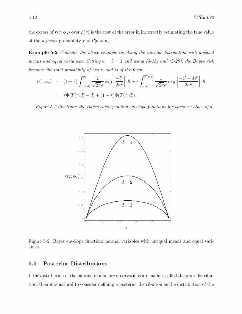
5-12 ECEn 672
the excess of r(τ, φα) over ρ(τ) is the cost of the error in incorrectly estimating the true value
of the a priori probability τ = P [θ = ϑ1].
Example 5-2 Consider the above example involving the normal distribution with unequal
means and equal variances. Setting a = b = 1 and using (5-18) and (5-20), the Bayes risk
becomes the total probability of error, and is of the form
r(τ, φτ) = (1 − τ)
∫ ∞
T (τ,d)
1√2πσ
exp
[−l2
2σ2
]
dl + τ
∫ T (τ,d)
−∞
1√2πσ
exp
[−(l − d)2
2σ2
]
dl
= τΦ(T (τ, d) − d) + (1 − τ)Φ(T (τ, d)).
Figure 5-2 illustrates the Bayes corresponding envelope functions for various values of d.
0 0.2 0.4 0.6 0.8 1
0
0.05
0.1
0.15
0.2
0.25
0.3
τ
r(τ, φτ )
d = 3
d = 2
d = 1
Figure 5-2: Bayes envelope function: normal variables with unequal means and equal vari-ances.
5.5 Posterior Distributions
If the distribution of the parameter θ before observations are made is called the prior distribu-
tion, then it is natural to consider defining a posterior distribution as the distribution of the
Winter 2009 5-13
parameter after observations are taken and processed. Let us proceed with this development
as follows.
We first consider the case for X and θ both continuous. Assuming we can reverse the
order of integration in (5-1), we obtain
r(τ, φ) =
∫
Θ
∫
XL[ϑ, φ(x)]fX|θ(x | ϑ)fθ(ϑ)dxdϑ
=
∫
X
∫
Θ
L[ϑ, φ(x)] fX|θ(x | ϑ)fθ(ϑ)︸ ︷︷ ︸
fXθ(x,ϑ)
dϑdx
=
∫
X
∫
Θ
L[ϑ, φ(x)]fθ|X(ϑ | x)dϑ
fX(x)dx, (5-24)
where we have used the fact that
fX|θ(x | ϑ)fθ(ϑ) = fXθ(x, ϑ) = fθ|X(ϑ | x)fX(x).
In other words, a choice of θ by the marginal distribution fθ(ϑ), followed by a choice of
X from the conditional distribution fX|θ(x | ϑ) determines a joint distribution of θ and X,
which in turn can be determined by first choosing X according to its marginal distribution
fX(x) and then choosing θ according to the conditional distribution fθ|X(ϑ | x) of θ given
X = x.
With this change in order of integration, some very useful insight may be obtained. We
see that we may minimize the Bayes risk given by (5-24) by finding a decision function φ(x)
that minimizes the inside integral separately for each x; that is, we may find for each x a
rule, call it φ(x), that minimizes
∫
Θ
L[ϑ, φ(x)]fθ|X(ϑ | x)dϑ. (5-25)
Definition. The conditional distribution of θ, given X, denoted fθ|X(ϑ | x), is called the
posterior, or a posteriori, distribution of θ.
The expression given in (5-25) is the expected loss given that X = x, and we may,
therefore, interpret a Bayes decision rule as one that minimizes the posterior conditional
expected loss, given the observation.

5-14 ECEn 672
The above results need be modified only in notation for the case where X and θ are dis-
crete. For example, if θ is discrete, say Θ = ϑ1, . . . , ϑk, we reverse the order of summation
and integration in (5-2) to obtain
r(τ, φ) =
k∑
i=1
∫
XL[ϑi, φ(x)]fX|θ(x | ϑi)fθ(ϑi)dx
=
∫
X
k∑
i=1
L[ϑi, φ(x)]fX|θ(x | ϑi)fθ(ϑi)dx
=
∫
X
k∑
i=1
L[ϑi, φ(x)]fθ|X(ϑi | x)
fX(x)dx. (5-26)
Example 5-3 Let us consider the simple hypothesis versus simple alternative problem for-
mulation, and let Θ = ϑ0, ϑ1 and ∆ = 0, 1. Assume we observe a random variable X
taking values in x0, x1, with the following conditional distributions:
fX|θ(x1|ϑ0) = P [X = x1 | θ = ϑ0] = 34, fX|θ(x0|ϑ0) = P [X = x0 | θ = ϑ0] = 1
4
fX|θ(x1|ϑ1) = P [X = x1 | θ = ϑ1] = 13, fX|θ(x0|ϑ1) = P [X = x0 | θ = ϑ1] = 2
3
The loss function for this problem is given by the matrix in Figure 5-3.
10 0
0 5
@@
@
∆Θ
0 1
ϑ0
ϑ1
Figure 5-3: Loss Function
Let P [θ = ϑ1] = τ and P [θ = ϑ0] = 1 − τ be the prior distribution for θ, for 0 ≤ τ ≤ 1.
We will address this problem by solving for the a posteriori pmf. The posterior pmf is given,
via Bayes theorem, as
fθ|X(ϑ1 | x) =fX|θ(x | ϑ1)fθ(ϑ1)
fX|θ(x | ϑ0)fθ(ϑ0) + fX|θ(x | ϑ1)fθ(ϑ1)
=
13τ
34(1−τ)+ 1
3τ
if x = x1
23τ
14(1−τ)+ 2
3τ
if x = x0
.
Winter 2009 5-15
Note that
fθ|X(ϑ0 | x) = 1 − fθ|X(ϑ1 | x).
After the value X = x has been observed, a choice must be made between the two actions
δ = 0 and δ = 1. The Bayes decision rule is
φτ(x) = arg minφ
L(ϑ1, φ)fθ|X(ϑ1 | x) + L(ϑ0, φ)fθ|X(ϑ0 | x)
=
arg minφ
L(ϑ1, φ)13τ
34(1−τ)+ 1
3τ
+ L(ϑ0, φ)34(1−τ)
34(1−τ)+ 1
3τ
if x = x1
arg minφ
L(ϑ1, φ)23τ
14(1−τ)+ 2
3τ
+ L(ϑ0, φ)14(1−τ)
14(1−τ)+ 2
3τ
if x = x0
, (5-27)
for φ ∈ 0, 1. Evaluating the expressions in braces in (5-27) yields, after using the values
for the loss function and some arithmetic,
φτ (x1) =
0 if τ ≤ 9
17
1 if τ > 917
and
φτ (x0) =
0 if τ ≤ 3
19
1 if τ > 319
.
We may compute the Bayes risk function as follows. If 0 ≤ τ < 319
, then it follows that
φτ (x) ≡ 0 will be the Bayes rule what ever the value of x. The corresponding Bayes risk is
0 · (1− τ)+10τ = 10τ . If 319
≤ τ ≤ 917
, then φτ (x0) = 1 and φτ (x1) = 0 is the Bayes decision
function, and the corresponding risk is
r(τ, φτ) = τR(ϑ1, φτ) + (1 − τ)R(ϑ0, φτ )
= τ [10 · 1
3+ 0 · 2
3] + (1 − τ)[0 · 3
4+ 5 · 1
4]
=10
3τ +
5
4(1 − τ).
If 917
< τ ≤ 1, then φτ (x) ≡ 1 is the Bayes rule, and the Bayes risk is 5(1 − τ). The Bayes
envelope function is provided in Figure 5-4.
5.6 Randomized Decision Rules
We have previously alluded to the existence of randomized decision rules, which we now
discuss in more detail. Suppose, rather than invoking a rule that assigns a specific action

5-16 ECEn 672
0.2 0.4 0.6 0.8 1
0.5
1
1.5
2
r(τ, φτ )
τ
Figure 5-4: Bayes envelope function
δ for a given x, we instead invoke a rule that attaches a specific probability distribution to
the actions, and the decision-maker then chooses its action by sampling the action space
according to that distribution. For example, let δ0 and δ1 be two candidate actions, and let
φ be a rule that yields, for each x, a probability α, such that the decision maker chooses
action δ1 with probability α and chooses action δ0 with probability 1 − α. Indeed, it is
easy to see that any finite convex combination of actions corresponds to a randomized rule.
In fact, even the deterministic rules we have been discussing can be viewed as degenerate
randomized rule, where we have set α = 1 for some action δ. Let D∗ denote the set of all
randomized decision rules. Let δ ∈ D and δ′ ∈ D be two rules, and let δα be the randomized
decision rule corresponding to choosing δ with probability α, where α ∈ (0, 1), and choosing
δ′ with probability 1 − α. Then δα ∈ D∗ and
R(ϑ, dα) = αR(ϑ, δ) + (1 − α)R(ϑ, δ′).

Winter 2009 5-17
5.7 Minimax Rules
An interesting approach to decision making is to consider ordering decision rules according
to the worst that could happen.
Consider the value τ = αM on the Bayes envelope plot given in Figure 5-1. At this value,
we have that
r(0, φαM) = r(1, φαM
) = maxτ
ρ(τ).
Thus, for τ = αM , the maximum possible expected loss due to ignorance of the true state
of nature is minimized by using φαM. This observation motivates the introduction of the
so-called minimax decision rules.
Definition. We say that a decision rule φ1 is preferred to rule φ2 if
maxϑ∈Θ
R(ϑ, φ1) < maxϑ∈Θ
R(ϑ, φ2).
Recall that D∗ is the set of all possible randomized decision rules; then this notion of pref-
erence leads to a linear ordering of the rules in D∗. A rule that is most preferred in this
ordering is called a minimax decision rule. That is, a rule φ0 is said to be minimax if
maxϑ∈Θ
R(ϑ, φ0) = minδ∈D∗
maxϑ∈Θ
R(ϑ, δ). (5-28)
The value on the right side of (5-28) is called the minimax value, or upper value of the game.
In words, (5-28) means, essentially, that if we first find the value of ϑ that maximizes
the risk for each rule φ ∈ D∗, then find the rule φ0 ∈ D∗ that minimizes the resulting set of
risks, we have the minimax decision rule. This rule corresponds to an attitude of “cutting
our losses.” We first determine what state nature would take if we were to take action φ and
it were perverse, then we take the action the minimizes the amount of damage that nature
can do to us.
If I am paranoid, I would be inclined toward a minimax rule. But, as they say, “Just
because I’m paranoid doesn’t mean they’re not out to get me,” and indeed nature may
have it in for me. In such a situation, nature would search through the family of possible
prior distributions, and would choose one that does me the most damage, even if I adopt a
minimax stance.

5-18 ECEn 672
Definition. A distribution τ0 ∈ Θ∗ is said to be a least favorable prior if
minδ∈D∗
r(τ0, δ) = maxτ∈Θ∗
minδ∈D∗
r(τ, δ). (5-29)
The value on the right side of (5-29) is called the maximin value, or lower value of the game.
The terminology, “least favorable,” derives from the fact that, if I were told which prior
nature was using, I would like least to be told a distribution τ0 satisfying (5-29), because
that would mean that nature had taken a stance that would allow me to cut my losses by
the least amount.
5.8 Summary of Binary Decision Problems
The following observations summarize the results we have obtained for the binary decision
problem.
1. Using either Neyman-Pearson or a Bayes criterion, we see that the optimum test is a
likelihood ratio test. Thus, regardless of the dimensionality of the observation space,
the test consists of comparing a scalar variable `(x) with a threshold.
2. In many cases construction of the likelihood ratio test can be simplified by using a
sufficient statistic.
3. A complete description of the likelihood ratio test performance can be obtained by
plotting the conditional probabilities PD versus PFA as the threshold is varied. The
resulting ROC curve can be used to calculate either the power for a given size (and
vice versa) or the Bayes risk (the probability of error).
4. The minimax criterion is a special case of a Bayes rule with a least favorable prior.
5. A Bayes rule minimizes the expected loss under the posterior distribution.
5.9 Multiple Decision Problems
Thus far, we have focused our discussion mainly on the binary hypothesis testing problem,
but we now turn our attention to the M-ary problem. Although [16, Page 46] claims the
generalization of Neyman-Pearson theory to multiple hypothesis exists but is not widely

Winter 2009 5-19
used, I have never seen another reference to it9. From its very construction, the Neyman-
Pearson theory is designed to deal with binary hypotheses; there does not seem to be a
natural extension to the problem of selecting from among M > 2 choices. Even granting
that a M-ary Neyman-Pearson theory exists, I suspect that it loses some of its elegance when
it is extended to more than the binary case. At any rate, we will not be attempting such
a generalization in this class; instead, we will pursue the Bayesian approach for arbitrary
finite Θ.
Suppose that Θ consists of k ≥ 2 points, Θ = ϑ1, . . . , ϑk, and consider the set, S, called
the risk set, contained in k-dimensional Euclidean space <k, of points of the form
R(ϑ1, δ), . . . , R(ϑk, δ),
where δ ranges through D∗, the set of all randomized decisions. In other words, S is the set
of all k-tuples y1, . . . , yk such that yi = R(ϑi, δ), i = 1, . . . , k, for some δ ∈ D∗.
Theorem 2 The risk set S is a convex subset of <k.
Proof. Let y = [y1, . . . , yk]T and y′ = [y′
1, . . . , y′k]
T be arbitrary points in S. According to
the definition of S, there exist decision rules δ and δ′ in D∗ for which yi = R(ϑi, δ) and
y′i = R(ϑi, δ
′) for i = 1, . . . , k. Let α be arbitrary such that 0 ≤ α ≤ 1 and consider the
decision rule δα which chooses rule δ with probability α and rule δ′ with probability 1 − α.
Clearly, δα ∈ D∗, and
R(ϑi, δα) = αR(ϑi, δ) + (1 − α)R(ϑi, δ′)
for i = 1, . . . , k. If z denotes the point whose i-th coordinate is R(ϑi, δα), then z = αy +
(1 − α)y′, thus z ∈ S. 2
A prior distribution for nature is a k-tuple of nonnegative numbers τ1, . . . , τk such that∑k
i=1 τi = 1, with the understanding that τi represents the probability that nature chooses
ϑi. Let τ = [τ1, . . . , τk]T . For any point y ∈ S, the Bayes risk is then the inner product
τ T y =
k∑
i=1
τiyi =
k∑
i=1
τiR(ϑi, δ).
9I think Van Trees is being kind with the phrase “not widely used.”
5-20 ECEn 672
(The existence of a randomized decision rule δ is guaranteed by the convexity of the risk
set.) We make the following observations:
1. There may be multiple points with the same Bayes risk (for example, suppose one or
more entries in τ is zero.) Consider the set of all vectors y that satisfy, for a given τ ,
the relationship
τ Ty = b (5-30)
for any real number b. Then all of these points (and the corresponding decision rules)
are equivalent.
2. The set of points y that satisfy (5-30) lie in a hyperplane; this plane is perpendicular
to the vector from the origin to the point (τ1, . . . , τk). To see this, consider Figure
5-5, where, for k = 2, the risk set and sets of equivalent points are displayed (the
concepts carry over to the general case for k > 2, but the graphical display is not as
convenient–or possible).
3. The quantity b can be visualized by noting that the point of intersection of the diagonal
line y1 = · · · = yk with the plane τ Ty =∑
i τiyi = b must occur at [b, . . . , b]T .
4. To find the Bayes rules we find the minimum of those values of b, call it b0, for which
the plane τ Ty = b0 intersects the set S. Decision rules corresponding to points in this
intersection are Bayes with respect to the prior τ .
We may also use the risk set to graphically depict the minimax point. The maximum
risk for a fixed rule δ is given by
maxi
R(ϑi, δ).
All points y ∈ S that yield this same value of maxi yi are equivalent with respect to the
minimax principle. Thus, all points on the boundary of the set
Qc = (y1, . . . , yk) : yi ≤ c for i = 1, . . . , k
for any real number c are equivalent. To find the minimax rules we find the minimum of those
values of c, call it c0, such that the set Qc0 intersects S. Any decision rule δ whose associated
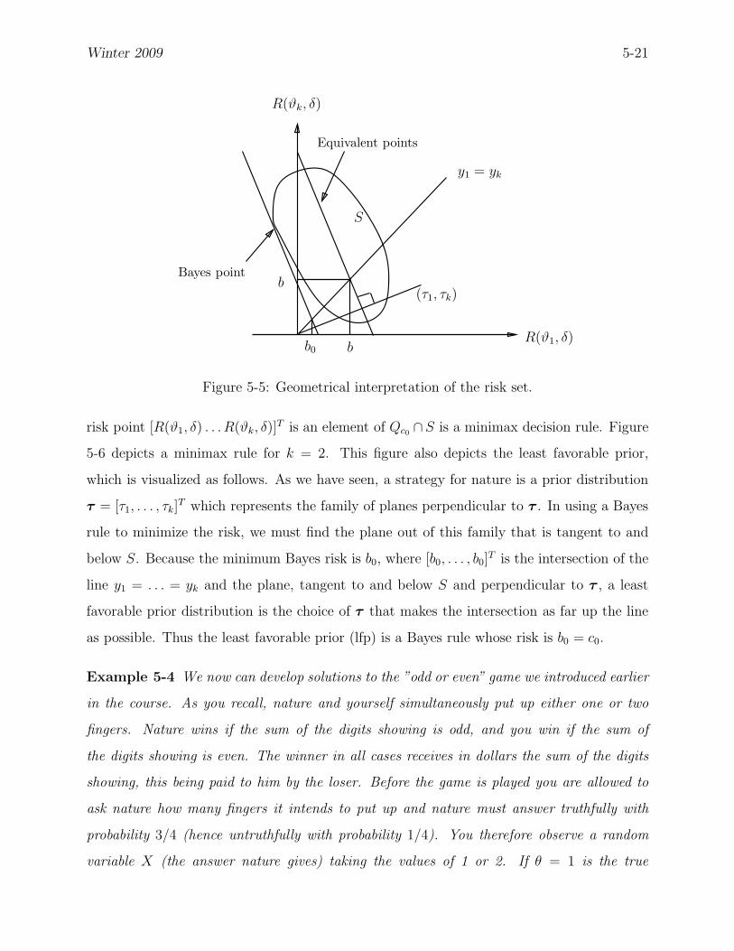
Winter 2009 5-21
b0 bR(ϑ1, δ)
(τ1, τk)b
S
Equivalent points
R(ϑk, δ)
Bayes point
y1 = yk
Figure 5-5: Geometrical interpretation of the risk set.
risk point [R(ϑ1, δ) . . . R(ϑk, δ)]T is an element of Qc0 ∩S is a minimax decision rule. Figure
5-6 depicts a minimax rule for k = 2. This figure also depicts the least favorable prior,
which is visualized as follows. As we have seen, a strategy for nature is a prior distribution
τ = [τ1, . . . , τk]T which represents the family of planes perpendicular to τ . In using a Bayes
rule to minimize the risk, we must find the plane out of this family that is tangent to and
below S. Because the minimum Bayes risk is b0, where [b0, . . . , b0]T is the intersection of the
line y1 = . . . = yk and the plane, tangent to and below S and perpendicular to τ , a least
favorable prior distribution is the choice of τ that makes the intersection as far up the line
as possible. Thus the least favorable prior (lfp) is a Bayes rule whose risk is b0 = c0.
Example 5-4 We now can develop solutions to the ”odd or even” game we introduced earlier
in the course. As you recall, nature and yourself simultaneously put up either one or two
fingers. Nature wins if the sum of the digits showing is odd, and you win if the sum of
the digits showing is even. The winner in all cases receives in dollars the sum of the digits
showing, this being paid to him by the loser. Before the game is played you are allowed to
ask nature how many fingers it intends to put up and nature must answer truthfully with
probability 3/4 (hence untruthfully with probability 1/4). You therefore observe a random
variable X (the answer nature gives) taking the values of 1 or 2. If θ = 1 is the true
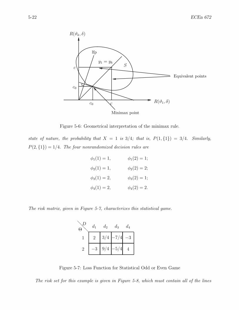
5-22 ECEn 672
c0 c
Minimax point
c0
c S
R(ϑk, δ)
R(ϑ1, δ)
Equivalent points
lfp
y1 = yk
Figure 5-6: Geometrical interpretation of the minimax rule.
state of nature, the probability that X = 1 is 3/4; that is, P (1, 1) = 3/4. Similarly,
P (2, 1) = 1/4. The four nonrandomized decision rules are
φ1(1) = 1, φ1(2) = 1;
φ2(1) = 1, φ2(2) = 2;
φ3(1) = 2, φ3(2) = 1;
φ4(1) = 2, φ4(2) = 2.
The risk matrix, given in Figure 5-7, characterizes this statistical game.
−3 9/4
2 3/4
−5/4
−7/4
4
−3
@@
@
DΘ
d1 d2 d3 d4
1
2
Figure 5-7: Loss Function for Statistical Odd or Even Game
The risk set for this example is given in Figure 5-8, which must contain all of the lines
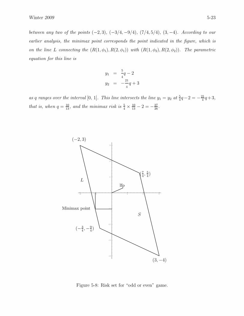
Winter 2009 5-23
between any two of the points (−2, 3), (−3/4,−9/4), (7/4, 5/4), (3,−4). According to our
earlier analysis, the minimax point corresponds the point indicated in the figure, which is
on the line L connecting the (R(1, φ1), R(2, φ1)) with (R(1, φ2), R(2, φ2)). The parametric
equation for this line is
y1 =5
4q − 2
y2 = −21
4q + 3
as q ranges over the interval [0, 1]. This line intersects the line y1 = y2 at 54q−2 = −21
4q+3,
that is, when q = 1013
, and the minimax risk is 54× 10
13− 2 = −27
26.
-2 -1 1 2 3
-4
-3
-2
-1
1
2
3
(−2, 3)
L
(74, 5
4)
(−34,−9
4)
(3,−4)
Minimax point
S
lfp
Figure 5-8: Risk set for “odd or even” game.

5-24 ECEn 672
We may compute the least favorable prior as follows. Let nature take action ϑ = 1 with
probability τ and ϑ = 2 with probability 1−τ . If the vector τ = [τ, 1−τ ]T is perpendicular to
L, the slope of this vector must be the negative of the reciprocal of the slope of L. Thus, we
require 1−ττ
= 37, or τ = 7
10. Thus, if nature chooses to hold up one finger 70% of the time,
it will maintain your expected loss to at least −2726
, and if you apply rule φ2 with probability
1013
and φ1 with probability 313
, you will restrict your average loss to no more than −2726
. It
seems reasonable to call −2726
the value of the game. If a referee were to arbitrate this game,
it would seem fair to require nature to pay you 2726
dollars in lieu of playing the game.
The above example demonstrates a situation in which the best you can do in response to
the worst nature can do yields the same expected loss as would be obtained if nature did its
worst in response to the best you can do. This result is summarized in the following theorem
(which we will not prove here).
Theorem 3 (The Minimax Theorem). If for a given decision problem (Θ, D, R) with finite
Θ = ϑ1, . . . , ϑk, the risk set S is bounded below, then
minδ∈D∗
maxτ∈Θ∗
r(τ, δ) = maxτ∈Θ∗
minδ∈D∗
r(τ, δ),
and there exists a least favorable distribution τ0.
This example demonstrates still another property of Bayes decision theory, which is,
essentially, that if we use a Bayes decision rule (that is, a rule that minimizes the Bayes
risk), we may restrict ourselves to nonrandomized rules. From our rules describing the
construction of the Bayes point for this problem, we see that every point on the line L is a
Bayes point, consequently the vertices (−2, 3) and (−34, −9
4) are Bayes points, corresponding
to nonrandomized decision rules. Can you construct the set of Bayes points corresponding
to every possible prior?
5.10 An Important Class of M-Ary Problems
Suppose there are M ≥ 2 possible source outputs, each of which corresponds to one of the M
hypotheses. We observe the output and are required to decide which source was used to gen-
erate it. Put in the light of the radar detection problem we discussed earlier, suppose there are

Winter 2009 5-25
M different target possibilities, and we not only have to detect the presence of a target, but
to classify it as well. For example, we may be required to choose between three alternatives:
H0 : no target present, H1 : target is present and hostile, H2 : target is present and friendly.
Formally, the parameter space Θ is of the form Θ = ϑ0, ϑ1, . . . , ϑM−1. Let H0 : θ =
ϑ0, , H1 : θ = ϑ1, . . . , HM−1 : θ = ϑM−1 denote the M hypotheses to test. We will employ
the Bayes criterion to address this problem, and assume that τ = [τ0, . . . , τM−1]T is the
corresponding a priori probability vector. We will denote the cost of each course of action
as Cij , where the first subscript i signifies that the i-th hypothesis is chosen, and the second
subscript j signifies that the j-th hypothesis is true. In words, Cij is the cost of choosing Hi
when Hj is true.
We observe a random variable X taking values in X ⊂ <k. We wish to generalize the
notion of a threshold test that was so useful for the binary case. Our approach will be to
compute the posterior conditional expected loss for X = x.
The natural generalization of the binary case is to partition the observation space into
M disjoint regions S0, . . . , SM−1, that is, X = S0 ∪ · · · ∪ SM−1, and to invoke a decision rule
of the form
φ(x) = n if x ∈ Sn, n = 0, . . . , M − 1. (5-31)
The loss function then assumes the form
L[ϑj , φ(x)] =
M−1∑
i=0
CijISi(x).
From (5-26), the Bayes risk is
r(τ, φ) =
∫
X
M−1∑
j=0
L[ϑj , φ(x)]fθ|X(ϑj | x)
fX(x)dx
=
∫
X
M−1∑
j=0
M−1∑
i=0
CijISi(x)fθ|X(ϑi | x)
fX(x)dx,
and we may minimize this quantity by minimizing the quantity in braces for each x. It
suffices to minimize the posterior conditional expected loss,
r′(τ, φ) =
M−1∑
j=0
M−1∑
i=0
CijISi(x)fθ|X(ϑi | x). (5-32)

5-26 ECEn 672
The problem reduces to determining the sets Si, i = 0, . . . , M − 1, that result in the mini-
mization of r′.
From Bayes rule, we have
fθ|X(ϑj | x) =fX|θ(x | ϑj)fθ(ϑj)
fX(x),
which when substituted into (5-32) yields
r′(τ, φ) =
M−1∑
j=0
M−1∑
i=0
CijISi(x)
fX|θ(x | ϑj)fθ(ϑj)
fX(x).
We now make a very important observation: Given X = x, we can minimize the posterior
conditional expected loss by minimizing
M−1∑
j=0
M−1∑
i=0
CijISi(x)fX|θ(x | ϑj)fθ(ϑj),
that is, fX(x) is simply a scale factor for this minimization problem, since x is assumed to
be fixed. Since
M−1∑
j=0
M−1∑
i=0
CijISi(x)fX|θ(x | ϑj)fθ(ϑj) =
M−1∑
i=0
ISi(x)
M−1∑
i=0
CijfX|θ(x | ϑj)fθ(ϑj),
we may now ascertain the structure of the sets Si that result in the Bayes decision rule φ(x)
given by (5-31).
Sk = x ∈ X :M−1∑
j=0
CkjfX|θ(x | ϑj)fθ(ϑj) ≤M−1∑
j=0
CijfX|θ(x | ϑj)fθ(ϑj) ∀i 6= k.
The general structure of these decision regions is rather messy to visualize and lengthy
to compute, but we can learn almost all there is to know about this problem by simplifying
it a bit. We first set
Cii = 0
Cij = 1, i 6= j.
Second, we consider only the case M = 3. Then, with τj = fθ(ϑj),
S0 = x : fX|θ(x|ϑ1)τ1+fX|θ(x|ϑ2)τ2 ≤ minfX|θ(x|ϑ0)τ0+fX|θ(x|ϑ2)τ2, fX|θ(x|ϑ0)τ0+fX|θ(x|ϑ1)τ1
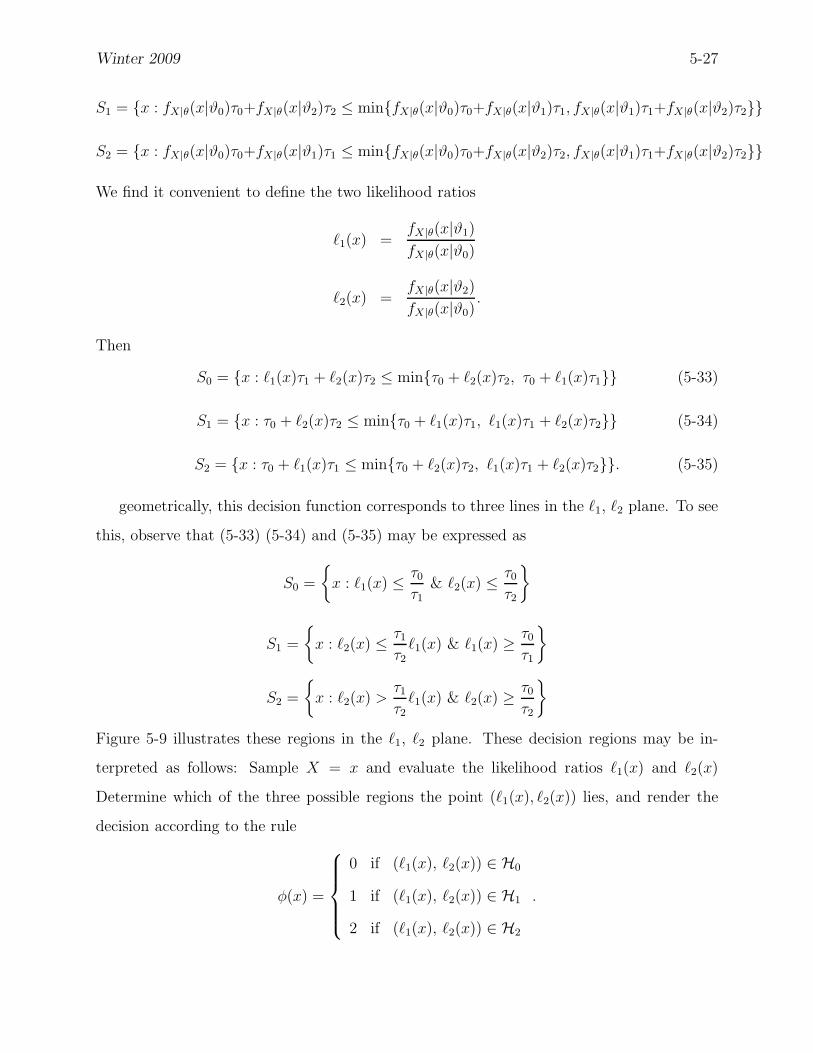
Winter 2009 5-27
S1 = x : fX|θ(x|ϑ0)τ0+fX|θ(x|ϑ2)τ2 ≤ minfX|θ(x|ϑ0)τ0+fX|θ(x|ϑ1)τ1, fX|θ(x|ϑ1)τ1+fX|θ(x|ϑ2)τ2
S2 = x : fX|θ(x|ϑ0)τ0+fX|θ(x|ϑ1)τ1 ≤ minfX|θ(x|ϑ0)τ0+fX|θ(x|ϑ2)τ2, fX|θ(x|ϑ1)τ1+fX|θ(x|ϑ2)τ2
We find it convenient to define the two likelihood ratios
`1(x) =fX|θ(x|ϑ1)
fX|θ(x|ϑ0)
`2(x) =fX|θ(x|ϑ2)
fX|θ(x|ϑ0).
Then
S0 = x : `1(x)τ1 + `2(x)τ2 ≤ minτ0 + `2(x)τ2, τ0 + `1(x)τ1 (5-33)
S1 = x : τ0 + `2(x)τ2 ≤ minτ0 + `1(x)τ1, `1(x)τ1 + `2(x)τ2 (5-34)
S2 = x : τ0 + `1(x)τ1 ≤ minτ0 + `2(x)τ2, `1(x)τ1 + `2(x)τ2. (5-35)
geometrically, this decision function corresponds to three lines in the `1, `2 plane. To see
this, observe that (5-33) (5-34) and (5-35) may be expressed as
S0 =
x : `1(x) ≤ τ0
τ1& `2(x) ≤ τ0
τ2
S1 =
x : `2(x) ≤ τ1
τ2`1(x) & `1(x) ≥ τ0
τ1
S2 =
x : `2(x) >τ1
τ2
`1(x) & `2(x) ≥ τ0
τ2
Figure 5-9 illustrates these regions in the `1, `2 plane. These decision regions may be in-
terpreted as follows: Sample X = x and evaluate the likelihood ratios `1(x) and `2(x)
Determine which of the three possible regions the point (`1(x), `2(x)) lies, and render the
decision according to the rule
φ(x) =
0 if (`1(x), `2(x)) ∈ H0
1 if (`1(x), `2(x)) ∈ H1
2 if (`1(x), `2(x)) ∈ H2
.
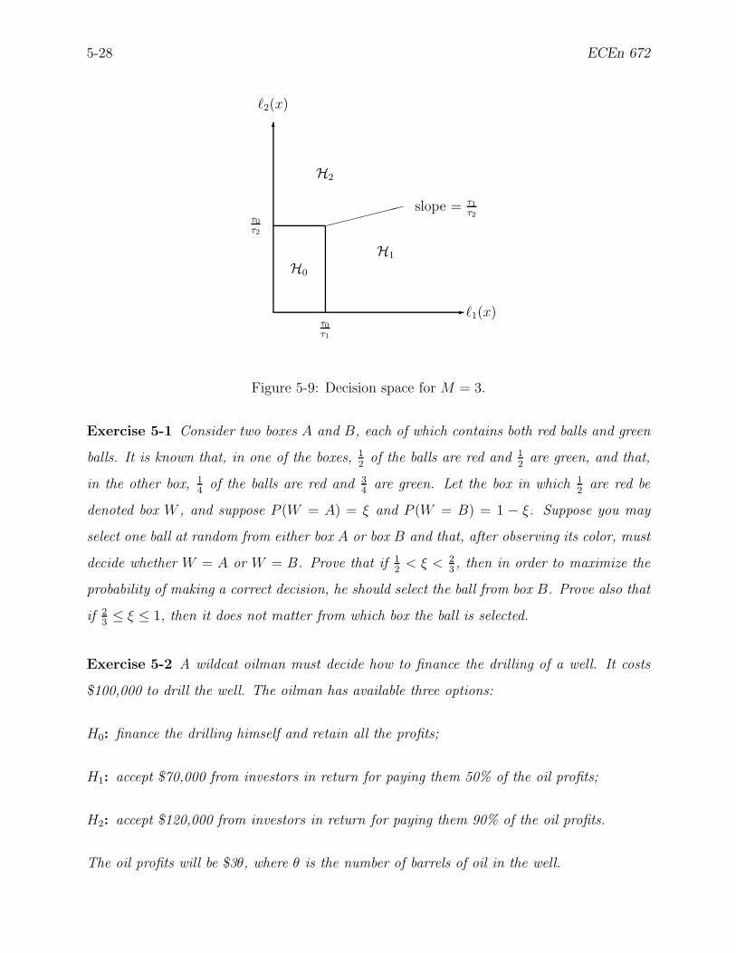
5-28 ECEn 672
- `1(x)
6
`2(x)
τ0τ1
τ0τ2
slope = τ1τ2
H0
H1
H2
Figure 5-9: Decision space for M = 3.
Exercise 5-1 Consider two boxes A and B, each of which contains both red balls and green
balls. It is known that, in one of the boxes, 12
of the balls are red and 12
are green, and that,
in the other box, 14
of the balls are red and 34
are green. Let the box in which 12
are red be
denoted box W , and suppose P (W = A) = ξ and P (W = B) = 1 − ξ. Suppose you may
select one ball at random from either box A or box B and that, after observing its color, must
decide whether W = A or W = B. Prove that if 12
< ξ < 23, then in order to maximize the
probability of making a correct decision, he should select the ball from box B. Prove also that
if 23≤ ξ ≤ 1, then it does not matter from which box the ball is selected.
Exercise 5-2 A wildcat oilman must decide how to finance the drilling of a well. It costs
$100,000 to drill the well. The oilman has available three options:
H0: finance the drilling himself and retain all the profits;
H1: accept $70,000 from investors in return for paying them 50% of the oil profits;
H2: accept $120,000 from investors in return for paying them 90% of the oil profits.
The oil profits will be $3θ, where θ is the number of barrels of oil in the well.
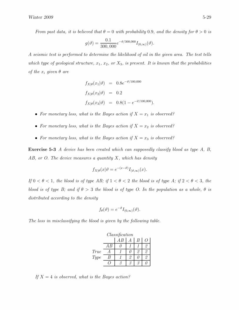
Winter 2009 5-29
From past data, it is believed that θ = 0 with probability 0.9, and the density for θ > 0 is
g(ϑ) =0.1
300, 000e−ϑ/300,000I(0,∞)(ϑ).
A seismic test is performed to determine the likelihood of oil in the given area. The test tells
which type of geological structure, x1, x2, or X3, is present. It is known that the probabilities
of the xi given θ are
fX|θ(x1|ϑ) = 0.8e−ϑ/100,000
fX|θ(x2|ϑ) = 0.2
fX|θ(x3|ϑ) = 0.8(1 − e−ϑ/100,000).
• For monetary loss, what is the Bayes action if X = x1 is observed?
• For monetary loss, what is the Bayes action if X = x2 is observed?
• For monetary loss, what is the Bayes action if X = x3 is observed?
Exercise 5-3 A device has been created which can supposedly classify blood as type A, B,
AB, or O. The device measures a quantity X, which has density
fX|θ(x|ϑ = e−(x−ϑ)I(ϑ,∞)(x).
If 0 < θ < 1, the blood is of type AB; if 1 < θ < 2 the blood is of type A; if 2 < θ < 3, the
blood is of type B; and if θ > 3 the blood is of type O. In the population as a whole, θ is
distributed according to the density
fθ(ϑ) = e−ϑI(0,∞)(ϑ).
The loss in misclassifying the blood is given by the following table.
ClassificationAB A B O
AB 0 1 1 2True A 1 0 2 2Type B 1 2 0 2
O 3 3 3 0
If X = 4 is observed, what is the Bayes action?

Winter 2009 6-1
6 Maximum Likelihood Estimation
As we have stated earlier, estimation is the process of making decisions over a continuum of
parameters. The same dichotomy exists here as with the detection problem, however, since
we may view the unknown parameter as either an unknown, but deterministic quantity,
or as a random variable. Consequently, there are multiple schools of thought regarding
estimation. In this section, we present the classical approach, based upon the principle of
maximum likelihood [1, 6, 16]. In a subsequent section we present an approach based upon
Bayesian assumptions.
6.1 The Maximum Likelihood Principle
The essential feature of the principle of maximum likelihood as it applies to estimation
theory is that is requires one to choose, as an estimate of a parameter, that value for which
the probability of obtaining a given sample actually observed is as large as possible. That
is, having obtained observations, one “looks back” and computes the probability, from the
point of view of one about to perform the experiment, that the given sample values will be
observed. This probability will in general depend on the parameter, which is then given that
value for which this probability is maximized10.
Suppose that the random variable X has a probability distribution which depends on a
parameter θ. Let fX(x | θ) denote, say, a pmf (it could be a pdf, we don’t really care for
now). We suppose that the form of fX is known, but not the value of θ. The joint pmf of m
sample random variables evaluated at the sample points x1, . . . , xm, is
l(θ, x1, . . . , xm) = fX1···Xm(x1, . . . , xm | θ) =m∏
i=1
fX(xi | θ) (6-1)
This function is also known as the likelihood function of the sample; we are particularly
interested in it as a function of θ when the sample values x1, . . . , xm are fixed. The principle
of maximum likelihood requires us to choose as an estimate of the unknown parameter that
value of θ for which the likelihood function assumes its largest value.
10This is reminiscent of story about the crafty politician who, once he observes which way the crowd isgoing, hurries to the front of the group as if to lead the parade.

6-2 ECEn 672
If the parameter θ is a vector, say θ = [θ1, . . . , θk]T , then the likelihood function will be
a function of all of the components of θ. Thus, we are free to regard θ as a vector in (6-1),
and the maximum likelihood estimate of θ is then the vector of numbers which render the
likelihood function a maximum.
Example 6-1 (A Maximum Likelihood Detector). Suppose you are given a coin and told
that it is biased, with one side four times as likely to turn up as the other; you are allowed
three tosses and must then guess whether it is biased in favor of head or in favor of tails.
Let θ be the probability of heads (H, with T corresponding to tails) on a single toss. Define
the random variable, X : H, T 7→ 0, 1; X(H) = 1 and X(T ) = 0. The pmf for X is
given byfX(0 | 4/5) = 1/5 fX(1 | 4/5) = 4/5;
fX(0 | 1/5) = 4/5 fX(1 | 1/5) = 1/5.
Suppose you throw the coin three times, resulting in the samples HTH. The sample values
are x1 = 1, x2 = 0, x3 = 1. The likelihood function is
l(θ, x1, x2, x3) = fX1X2X3(x1, x2, x3 | θ)
= fX1X2X3(1, 0, 1 | θ)
= fX1(1 | θ)fX2(0 | θ)fX3(1 | θ)
or
l(4/5, 1, 0, 1) = (4/5)(1/5)(4/5) = 16/125
l(1/5, 1, 0, 1) = (1/5)(4/5)(1/5) = 4/125
Clearly, θ = 4/5 yields the larger value of the likelihood function, so by the likelihood principle
we are compelled to decide that the coin is biased in favor of heads.
Although, as this example demonstrates, the principle of maximum likelihood may be
applied to discrete decision problems, it has found greater utility for problems where the
distribution is continuous and differentiable in θ. The reason for this is that we will usually
be taking derivatives in order to find maxima. But it is important to remember that general

Winter 2009 6-3
decision problems can, in principle, be addressed via the principle of maximum likelihood.
Notice, for this example, that neither cost functions nor a prior knowledge of the distribution
of the parameters is needed to fashion a maximum likelihood estimate.
Example 6-2 (Empiric Distributions). Let X be a random variable of unknown distribu-
tion, and that X1, . . . , Xm are sample random variables from the population of X. Suppose
we are required to estimate the distribution function of X. There are many ways to approach
this problem. One way would be to assume some general structure, such as an exponential
family, and try to estimate the parameters of this family. But then one has the simultaneous
problems of (a) estimating the parameters and (b) justifying the structure. Although there are
many ways of doing both of these problems, it is not easy. The maximum likelihood method
gives us a fairly simple approach that, if for no other reason, would be valuable as a baseline
for evaluating other, more sophisticated approaches.
To apply the principle of maximum likelihood to this problem, we must first define the
parameters. We do this by setting
θi = P [Xi = xi], , i = 1, . . . , m.
The event
[X1 = x1, · · · , Xm = xm]
is observed, and, according to the maximum likelihood principle, we wish to choose the values
of θi that maximize the probability that this event will occur. Since the events [Xi = xi], i =
1, . . . , m are independent, we have
P [X1 = x1, · · · , Xm = xm] =
m∏
i=1
P [Xi = xi] =
m∏
i=1
θi,
which we wish to maximize subject to the constraint∑m
i=1 θi = 1. The standard way to
extremize a function subject to constraints is to formulate it as a Lagrange multiplier problem.
Let
J =
m∏
i=1
θi + λ(
m∑
i=1
θi − 1),

6-4 ECEn 672
and set the gradient of J with respect to θi, i = 1, . . . , m and with respect to λ to zero:
∂J
∂θj=
∏
i6=j
θi + λ = 0, j = 1, . . . , m
∂J
∂λ=
m∑
i=1
θi − 1 = 0
But the only way all of the products∏
i6=j θi can be equal is if θ1 = · · · = θm, and the
constraint therefore requires that θi = 1/m, i = 1, . . . , m.
We define the maximum likelihood estimate for the distribution as follows. Let X be a
random variable, called the empiric random variable, whose distribution function is
FX(x) = P [X ≤ x] =1
m
m∑
i=1
I[xi,∞)(x)
Figure 6-1 illustrates the structure of the empiric distribution function.
+ xx2 x1 x5x3 x4
1m
2m
mm
FX(x)
Figure 6-1: Empiric Distribution Function.
For large samples, it is convenient to quantize the observations and construct the empiric
density function by building a histogram.
Thus, the empiric distribution is precisely that distribution for which the influence of the
sample values actually observed is maximized at the expense of other possible values of X.
Of course, the actual utility of this distribution is limited since the number of parameters
may be very large. But it is a maximum likelihood estimate of the distribution function.

Winter 2009 6-5
6.2 Maximum Likelihood for Continuous Distributions
Suppose now that the random variable X is continuous and has a probability density function
fX(x | θ) which depends on the parameter θ (θ may be a vector). The joint probability density
function of the sample random variables, evaluated at the sample points x1, . . . , xm, is given
by
l(θ, x1, . . . , xm) = fX1···Xm(x1, . . . xm | θ) =m∏
i=1
fX(xi | θ).
For small dx1, . . . , dxm, the m + 1-dimensional volume fX1···Xm(x1, . . . xm | θ)dx1 · · · dxm rep-
resents, approximately, the probability that a sample will be chosen for which the sample
points lie within an n-dimensional rectangle at x1, . . . , xm, with sides dx1, . . . , dxm. Con-
ceptually, we can consider calculating this volume, for fixed xi and dxi, as θ is varied over
its range of permissible values. According to the maximum likelihood principle, we take,
as the maximum likelihood estimate of θ, that value that maximizes the volume, the idea
being that, if that were the actual value of θ that nature used, it would correspond to the
distribution that yields the largest probability of producing samples near the observed values
x1, . . . , xm. Since the rectangle is fixed, the volume, and hence the probability, is maximized
by maximizing the likelihood function l(θ, x1, . . . , xm).
It must be stressed that the likelihood function l(θ, x) is to be viewed as a function of
θ, with x being a fixed quantity, rather than a variable. This is in contradistinction to the
way we view the density function fX(x | θ), were θ is a fixed quantity and x is viewed as a
variable. So remember, even though we may write l(θ, x) = fX(x | θ) we view the roles of x
and θ in the two expressions entirely differently.
It is actually more convenient, for many applications, to consider the logarithm of the
likelihood function, which we denote
L(θ, x) = log fX(x | θ),
and call the log-likelihood function. Since the logarithm is a monotonic function, the maxi-
mization of the likelihood and log-likelihood functions is equivalent, that is, θML maximizes
the likelihood function if and only if it also maximizes the log-likelihood function. Thus, in
this development we will deal mainly with the log-likelihood function.

6-6 ECEn 672
If the log-likelihood function is differentiable in θ, a necessary but not sufficient condition
for θ to be a maximum of the log-likelihood function is for the gradient of the log-likelihood
function to vanish at that value of θ, that is, we require
∂
∂θL(θ, x) =
∂
∂θlog fX(x | θ) = 0.
The major issue before us is to find a way to maximize the likelihood function. If the
maximum is interior to the range of θ, and and L(θ, x) has a continuous first derivative, then
a necessary condition for θML to be the maximum likelihood estimate for θ is that
∂L(θ, x)
∂θ
∣∣∣∣θ=θML
= 0. (6-2)
This equation is called the likelihood equation. We now give some examples to illustrate the
maximization process.
Example 6-3 Let X1, . . . , Xm denote a random sample of size m from a uniform distri-
bution over [0, θ]. We wish to find the maximum likelihood estimate of θ. The likelihood
function is
l(θ, x1, . . . , xm) = θ−m
m∏
i=1
I(0,θ)(xi)
= θ−mm∏
i=1
I(0,maxixi)(mini
xi)I(minixi,θ)(maxi
xi)
= θ−m
m∏
i=1
I(minixi,θ)(maxi
xi)
= θ−mm∏
i=1
I(maxixi,∞)(θ).
Since the maximum of this quantity does not occur on the interior of the range of θ, we can’t
take derivatives and set to zero. But we don’t need to do that for this example, since θ−m is
monotonically decreasing in θ. Consequently, the likelihood function is maximized at
θML = maxi
xi.

Winter 2009 6-7
Example 6-4 Let X1, . . . , Xm denote a random sample of size m from the normal distribu-
tion N (µ, σ2). We wish to find the maximum likelihood estimates for µ and σ2. The density
function is
fX1,...,Xm(x1, . . . , xm |µ, σ) =
m∏
i=1
1√2πσ
exp
[
−(xi − µ)2
2σ2
]
,
and the log-likelihood function is then
L(µ, σ, x1, . . . , xm) = −m log√
2π − m log σ − 1
2σ2
m∑
i=1
(xi − µ)2.
Taking the gradient and equating to zero yields
∂L
∂µ=
1
σ2
m∑
i=1
(xi − µ) = 0
⇒ µML =1
m
m∑
i=1
xi,
and
∂L
∂σ= −m
σ+ σ−3
m∑
i=1
(xi − µ)2 = 0
⇒ σ2ML =
1
m
m∑
i=1
(xi − µ)2.
Before we get too euphoric over the simplicity and seemingly magical powers of the
maximum likelihood approach, consider the following example.
Example 6-5 Let X1 ∼ N (θ, 1) and X2 ∼ N (−θ, 1) and define
Y =
X1 with probability 1/2
X2 with probability 1/2.
then
fY (y | θ) =1
2
1√2π
e−12(y−θ)2 +
1
2
1√2π
e−12(y+θ)2 .
Now let Y = y′ be a given sample value. According to our procedure, we would evaluate the
likelihood function at y′, yielding
l(θ, y′) =1
2
1√2π
e−12(y′−θ)2 +
1
2
1√2π
e−12(y′+θ)2 ,
6-8 ECEn 672
and choose, as the maximum likelihood estimate of θ, that value that maximizes l(θ, y′). But
this function does not have a unique maximum, so there is not a unique estimate. Both
θML = y′ and θML = −y′ qualify as maximum likelihood estimates for θ.
6.3 Comments on Estimation Quality
In the immortal words of A. Jazwinski, “An estimate is meaningless unless one knows how
good it is [8, Page 150].” Thus, estimation theorists are sometimes consumed, not only
with devising and understanding various algorithms for estimation, but with evaluations of
how reliable they are. We usually ask the question in the superlative: “What is the best
estimate?”
We might be tempted to answer that the best estimate is the one closest to the true value
of the parameter to be estimated. But every estimate is a function of the sample values,
and thus is the observed value of some random variable. There is no means of predicting
just what the individual values are to be for any given experiment, so the goodness of an
estimate cannot be judged reliably from individual values. As we repeatedly sample the
population, however, we may form statistics, such as the sample mean and variance, whose
distributions we may calculate. If we are able to form estimators from these statistics, then
the best we can hope for is that the bulk of the mass in the distribution is concentrated in
some small neighborhood of the true value. In such circumstances, there is a high probability
that the estimate will only differ from the true value by a small amount. From this point of
view, we may order the quality of estimators as a function of how the sample distribution is
concentrated about the true value.
If the distribution is such that the mathematical expectation of estimate is exactly the
true value, then the estimator is, of course, unbiased. In general, we would prefer unbiased
estimates, and will restrict our attention primarily to such estimators in the sequel.
One measure of the dispersion of a distribution is its variance (or covariance, in the multi-
dimensional case). Most estimation techniques use this measure exclusively as a means of
evaluating the quality of the estimate. This choice is motivated strongly by the important
case when the sampling distributions of the estimates are at least approximately normal,
since then the second-order moment is then the unique measure of dispersion.

Winter 2009 6-9
Based upon the above arguments, we should feel justified in focusing primarily on the
variance of the estimation error as the measure of dispersion and, hence, of goodness. But
I want to sensitize you to the fact that this is a somewhat arbitrary, albeit very reasonable,
measure of goodness, and later in this course I hope to revisit these issues in a little more
depth, and build a case for measures other than dispersion as being valid measures of quality.
But for now, we will follow the conventional development and focus on the measure of quality
being equivalent to measures of dispersion, that is, to the variance of the estimation error.
6.4 The Cramer-Rao Bound
The maximum likelihood method of estimation does not provide, as a byproduct of calculat-
ing the estimate, any measure of the concentration (that is, the variance) of the estimation
error. Although the variance can be calculated for many important examples, it is difficult
for others. Rather than approach the problem of calculating the variance for an estimate
directly, therefore, we will first calculate a lower bound for the variance of the estimation er-
ror for any unbiased estimator, then we will see how the variance of the maximum likelihood
estimation error compares with this lower bound.
Before stating the main result of this section, we need to establish some new notation and
terminology and prove some preliminary results. A good modern reference for this material
is [11], from whom the following development is borrowed. I think it is a better development,
since it proves the main results for the vector case in a very nice way. You may contrast this
development with the more conventional proofs given in [16].
The Score Function and Fisher Information
Definition. Let X = [X1, . . . , Xn]T denote an n-dimensional random vector, and θ =
[θ1, . . . , θp]T denote a p-dimensional parameter vector. The score function s(θ,X) of a like-
lihood function l(θ,X) is defined as
sT (θ,X) =∂
∂θL(θ,X) =
1
l(θ,X)
∂
∂θl(θ,X).
More on notation: since the likelihood and log-likelihood functions are scalars and θ is a
p-dimensional vector, then s is the p-dimensional column matrix
s(θ,X) =
[∂
∂θ1L(θ,X), . . . ,
∂
∂θpL(θ,X)
]T
.

6-10 ECEn 672
Before continuing, we prove some useful facts about the score function. We begin with
the following theorem.
Theorem 1 If s(θ,X) is the score of a likelihood function l(θ,X) and if t is any vector-
valued function of X and θ, then (under certain regularity conditions)11
Es(θ,X)tT (θ,X) =∂
∂θEtT (θ,X) − E
(∂
∂θtT (θ,X)
)
. (6-3)
Proof. We have
EtT (θ,X) =
∫
tT (θ,x)fX(x | θ)dx
=
∫
tT (θ,x)l(θ,x)dx.
Upon differentiating both sides with respect to θ and taking the differentiation under the
integral sign in the right-hand side (this is were the regularity conditions come into play),
we obtain
∂
∂θEtT (θ,X) =
∫∂ log l(θ,x)
∂θtT (θ,x)l(θ,x)dx +
∫∂tT (θ,x)
∂θl(θ,x)dx. (6-4)
The result follows on simplifying and rearranging this expression. 2
We may quickly obtain three useful corollaries of this theorem.
Corollary.
If s(θ,X) is the score corresponding to a regular likelihood function l(θ,X), then
Es(θ,X) = 0. (6-5)
Proof. Choose t as any constant vector. Then, , since t is not a function of θ, its derivative
vanishes, so by (6-3),
Es(θ,X)tT = E[s(θ,X)]tT = 0,
which can happen for arbitrary t only if E[s(θ,X)] = 0. 2
11This is nice way of saying that we will assume whatever additional assumptions may be required toaccomplish all of the steps outlined in the proof. This isn’t too bad of a cop-out, since the regularityconditions turn out to be quite mild.
Winter 2009 6-11
Corollary.
If s(θ,X) is the score corresponding to a regular likelihood function l(θ,X) and if t(X)
is any unbiased estimator of θ, then
E[s(θ,X)tT (X)] = I. (6-6)
Proof. Since the estimate is unbiased, we have Et(X) = θ, and since t is not a function of
θ, we have ∂tT
∂θ= 0, thus by (6-3)
E[s(θ,X)tT (X)] =∂θ
∂θ= I.
2
The Cramer-Rao Lower Bound
Definition. The covariance matrix of the score function is the Fisher information matrix,
denoted J(θ). Since by (6-5) the score function is zero-mean, we have
J(θ) = Es(θ,X)sT (θ,X). (6-7)
Theorem 2 (Cramer-Rao). If t(X) is any unbiased estimator of θ based on a regular
likelihood function, then
E[t(X) − θ][t(X) − θ]T ≥ J−1(θ), (6-8)
where J(θ) is the Fisher information matrix.
Proof.
For brevity, let Var [t] = E[t(X) − θ][t(X) − θ]T . Let a and c be two p-dimensional
vectors and let s(θ,X) be the score function. Form the two random variables α = aT t(X)
and β = cT s(θ,X). Since the correlation coefficient,
ραβ =Eαβ
√
Var [α]Var [β]
is bounded in magnitude by one, we have that
E2(αβ)
Var [α]Var [β]≤ 1. (6-9)

6-12 ECEn 672
But since the score function is zero mean, it is immediate that
Var [β] = EcT s(θ,X)sT (θ,X)c
= cT Var [s(θ,X)]c
= cTJ(θ)c.
Also,
Var [α] = aT Var [t]a.
Furthermore, by (6-6) we have that
Eαβ = aT E[t(X)sT (θ,X)]c
= aT Ic
= aT c.
Substituting these expressions into (6-9),
E2(αβ)
Var [α]Var [β]=
(aTc)2
aT Var [t]acTJ(θ)c≤ 1. (6-10)
The reason we have set up this equation is because we want to exploit a little trick (that
about fifty years of hindsight have provided the community when solving problems of this
type). The trick is, we want to apply a certain neat little result that we now develop (this is
worth remembering). Suppose you are given two vectors, a and c, and wish to maximize the
projection of one vector onto another, subject to a constraint on one of the vectors, say, c, is
of the form cTJc = 1, where J is a positive definite matrix. This particular quadratic form
corresponds to the Mahalanobis length of the vector c. In other words, we want to constrain,
in some general sense, the length of c and still align it as best we can along the direction
defined by a. The answer is provided by the following lemma.
Lemma 2 Let J be a positive definite matrix, and let a be a fixed vector. The maximum of
aT c subject to the constraint
cTJc = 1 (6-11)
is attained at
c =J−1a
(aTJ−1a)12
.

Winter 2009 6-13
Proof of Lemma. We formulate this maximization problem as a Lagrange multiplier problem:
C(c, λ) = aT c + λ(cTJc − 1),
and differentiate C with respect to c and λ, set the results to zero, and solve for the unknowns.
∂C
∂c= a + 2λcTJ = 0 (6-12)
∂C
∂λ= cTJc − 1 = 0. (6-13)
Solving (6-12) for c yields
c =J−1a
2λ,
and substituting this into (6-13) yields
2λ =√
aT J−1a.
Thus, the extremizing value is given by
c =J−1a√aT J−1a
.
This proves the lemma.
Substituting this result into (6-10) and applying the constraint (6-11) yields
(
aT J−1(θ)a√aT J−1(θ)a
)2
aT Var [t]a=
aT J−1(θ)a
aT Var [t]a≤ 1. (6-14)
We now observe that this inequality must hold for all a, so
aTVar [t] − J−1(θ)
a ≥ 0
for all a, which is equivalent to (6-8). 2
The inverse of the Fisher information matrix is therefore a lower bound on the variance
that may be attained by any unbiased estimator of the parameter θ given the observations
X. It is important to determine conditions under which Cramer-Rao lower bound may be
achieved. From (6-9) we see that equality is possible if
E2(αβ) = Var [α]Var [β],

6-14 ECEn 672
or
E(αβ) =√
Var [α]√
Var [β].
But from the Schwarz inequality, equality is possible if and only if α and β are linearly
related, that is, if
t(X) = k(θ)s(θ,X).
Efficiency
Definition. An estimator is said to be efficient if it is unbiased and the covariance of the
estimation error equals the Cramer-Rao lower bound, that is, let θ = t(X) be an estimator
for θ. Then θ is efficient if
Eθ = θ
E[θ − θ][θ − θ]T = J−1(θ).
Theorem 3 (Efficiency) An unbiased estimator θ is efficient if and only if
J(θ)(θ − θ) = s(θ,X). (6-15)
Furthermore, any unbiased efficient estimator is a maximum likelihood estimator.
Proof. Suppose J(θ)(θ − θ) = s(θ,X). Then from the definition
J(θ) = Es(θ,X)sT (θ,X)
= J(θ)E[θ − θ][θ − θ]TJ(θ).
But this result implies E[θ − θ][θ − θ]TJ(θ) = I, which yields efficiency.
Conversely, suppose θ is efficient. From (6-5) and (6-6), it follows that
Es(θ,X)(θ − θ)T = I,
so by the Schwarz inequality,
I =
Es(θ,X)(θ − θ)T2
≤ E[s(θ,X)sT (θ,X)]E[(θ − θ)(θ − θ)T ]
= J(θ)E(θ − θ)(θ − θ)T = I by efficiency assumption.

Winter 2009 6-15
Equality can hold with the Schwartz inequality if and only if
s(θ,X) = K(θ)(θ − θ)
for some constant K(θ). Multiplying both sides of this expression by (θ − θ)T and taking
expectations yields K(θ) = J(θ).
To show that any unbiased efficient estimator is a maximum likelihood estimator, let θ
be efficient and unbiased, and let θ be a maximum likelihood estimate of θ. Evaluating
(6-15) at θ = θ yields
J(θ)(θ − θ) = s(θ,X).
but the score function is zero when evaluated at the maximum likelihood estimate, conse-
quently,
θ = θ.
2
6.5 Asymptotic Properties of Maximum Likelihood Estimators
Unfortunately, it is the exception rather than than the rule that an unbiased efficient estima-
tor can be found for problems of practical importance. This fact motivates us to analyze just
how close we can get to the ideal of an efficient estimate. Our approach will be to examine
the large sample properties of maximum likelihood estimates.
In our preceding development we have consider the size of the sample as a fixed integer
m ≥ 1. Let us now suppose that an unbiased estimate can be defined for all m, and consider
the asymptotic behavior of θML as m tends to infinity. In this section we establish three
key results (subject to sufficient regularity of the distributions): (a) maximum likelihood
estimates are consistent, (b) maximum likelihood estimates are asymptotically normally dis-
tributed, and (c) maximum likelihood estimates are asymptotically efficient. In the interest
of clarity, we will treat only the case for scalar θ. We assume, in the statement of the
following three theorems, that all of the appropriate regularity conditions are satisfied.
Definition. Let θm be an estimator based on m samples of a random variable. The sequence
θm, m = 1, . . . ,∞ is said to be a consistent sequence of estimators of θ if limm→∞ θm = θ

6-16 ECEn 672
almost surely, (that is, with probability one), written
θma.s.−→ θ.
Theorem 4 (Consistency) Let θm designate the maximum likelihood estimate of θ based on
m independent, identically distributed random variables X1, . . . , Xm. Then, if θ0 is the true
value of the parameter, θm converges almost surely to θ0.
Proof. Although this theorem is true in a very general setting, its rigorous proof is beyond
the scope of our preparation. Consequently, we will content ourselves with a heuristic demon-
stration, based on [4]. For our demonstration, we will proceed through all of the major steps
of the proof, but will assume sufficient regularity and other nice properties, when needful,
to make life bearable.
To simplify things, let x = x1, . . . , xm, and introduce the the following notation.
fm(x | θ) def= fX1,...,Xm(x1, . . . , xm | θ).
We can get away with this since the quantities x1, . . . , xm do not change throughout the
proof. Rather, the parameter that changes is θ.
From Theorem 1 and its corollaries,
E
[∂ log fm(X | θ)
∂θ
]
= 0, (6-16)
where X = X1, . . . , Xm.Suppose the true value of the parameter θ is θ0. Now let us expand
∂ log fm(x | θ)∂θ
in a
Taylor series about θ0 to obtain
∂ log fm(x | θ)∂θ
∣∣∣∣θ=θ′
=∂ log fm(x | θ)
∂θ
∣∣∣∣θ=θ0
+∂2 log fm(x | θ)
∂θ2
∣∣∣∣θ=θ∗
(θ′ − θ0), (6-17)
where θ∗ is chosen to force equality. Let θm be the maximum likelihood estimate based on
X1, . . . , Xm, which consequently satisfies
∂ log fm(x | θ)∂θ
∣∣∣∣θ=θm
= 0.

Winter 2009 6-17
Hence, evaluating (6-17) at θ′ = θm, we obtain
∂2 log fm(x | θ)∂θ2
∣∣∣∣θ=θ∗
(θm − θ0) = − ∂ log fm(x | θ)∂θ
∣∣∣∣θ=θ0
(6-18)
Since X1, . . . , Xm are i.i.d., we have, with fX(x | θ) the common density function,
∂ log fm(x | θ)∂θ
=∂
∂θlog
m∏
i=1
fX(xi | θ)
=∂
∂θ
m∑
i=1
log fX(xi | θ)
=m∑
i=1
∂ log fX(xi | θ)∂θ
.
By a similar argument,
∂2 log fm(x | θ)∂θ2
=m∑
i=1
∂2 log fX(xi | θ)∂θ2
.
From the strong law of large numbers12 it follows that
1
m
m∑
i=1
∂ log fX(xi | θ)∂θ
a.s−→ E
[∂ log fX(X | θ)
∂θ
]
= 0, (6-19)
where the last equality holds from (6-16). Similarly,
1
m
m∑
i=1
∂2 log fX(xi | θ)∂θ2
∣∣∣∣∣θ=θ∗
a.s−→ E
[∂2 log fX(X | θ)
∂θ2
]
θ=θ∗. (6-20)
We now make the assumption that
E
[∂2 log fX(X | θ)
∂θ2
]
θ=θ∗6= 0.
This assumption is essentially equivalent to the condition that the likelihood function be a
concave function for all values of θ. We might suspect that most of the common distributions
we would use satisfy this condition–but we will not expend the effort to prove it. Given the
above assumption and substituting (6-19) and (6-20) into (6-18), we obtain that
(θm − θ0)a.s.−→
E[
∂ log fX(X | θ)∂θ
]
θ=θ0
E[
∂2 log fX(X | θ)∂θ2
]
θ=θ∗.
= 0. (6-21)
12The strong law of large numbers says that for Xi a sequence of i.i.d. random variables with common
expectation µ, then 1
n
∑n
i=1xi
a.s−→ µ.

6-18 ECEn 672
2
The above theorem shows that, as m → ∞, the maximum likelihood estimate θm tends
to θ0 with probability one, the true value of the parameter. The next theorem shows us
that, for large m, the values of θm from different trials are clustered around θ0 with a normal
distribution.
Theorem 5 (Asymptotic normality) Let θm designate the maximum likelihood estimate of
θ based on m independent, identically distributed random variables X1, . . . , Xm. Then if θ0
is the true value of the parameter, θm converges in law to a normal random variable, that is,
√m(θm − θ0)
law−→ Y,
where
Y ∼ N (0, J−1(θ0)),
where J(θ) the Fisher information.
Proof. Due to the complexity of the proof of this result, we content ourselves with a heuristic
demonstration of this result also.
First, we form a Taylor expansion about the true parameter value, θ0:
∂ log fm(x | θ)∂θ
∣∣∣∣θ=θm
=∂ log fm(x | θ)
∂θ
∣∣∣∣θ=θ0
+∂2 log fm(x | θ)
∂θ2
∣∣∣∣θ=θ0
(θm − θ0) + h.o.t. (6-22)
Since θma.s.−→ θ0, we assume sufficient regularity to neglect the higher order terms. Also, since
θm is the maximum likelihood estimate, the left-hand side of (6-22) is zero, and therefore
1√m
∂ log fm(x | θ)∂θ
∣∣∣∣θ=θ0
= −√
m
m
∂2 log fm(x | θ)∂θ2
∣∣∣∣θ=θ0
(θm − θ0). (6-23)
But from the strong law of large numbers,
1
m
∂2 log fm(x | θ)∂θ2
a.s.−→ E
[∂2 log fX(X | θ)
∂θ2
]
. (6-24)
From Theorem 1 with t = s, we obtain
Es(θ,X)sT (θ,X) = −E
(∂
∂θsT (θ,X)
)
= −E
(∂2
∂θ∂θL(θ,X)
)
,

Winter 2009 6-19
or, rewriting,
E
[∂2 log fX(X | θ)
∂θ2
]
= E
[∂ log fX(X | θ)
∂θ
]2
= J(θ). (6-25)
We have thus established that the random variable
∂ log fX(Xi | θ)∂θ
∣∣∣∣θ=θ0
is a zero-mean random variable with variance J(θ0). Thus, by the central limit theorem13
the left-hand side of (6-23) converges to a normal random variable, that is,
1√m
m∑
i=1
∂ log fX(Xi | θ)∂θ
∣∣∣∣θ=θ0
law−→ W,
where W ∼ N [0, J(θ0)]. Consequently, the right-hand side of (6-23) also converges to W ,
that is,
√mJ(θ0)(θm − θ0)
law−→ W.
Finally, it is evident, therefore, that
√m(θm − θ0)
law−→ 1
J(θ0)W ∼ N [0, J−1(θ0)]. (6-26)
2
Theorem 6 (Asymptotic efficiency) Within the class of consistent uniformly asymptotically
normal estimators, θm is asymptotically efficient in the sense that asymptotically it attains
the Cramer-Rao lower bound as m → ∞.
Proof. This result is an immediate consequence of the previous theorem and the Cramer-Rao
lower bound. 2
This theorem is of great practical significance, since it shows that the maximum likelihood
estimator makes efficient use of all the available data for large samples.
13The version of the central limit theorem we need is: Let Xn be a sequence of i.i.d. random variableswith common expectation µ and common variance σ2. Let Zn = X1+···+Xn−nµ
√nσ
. Then Zn → Z where Z is
distributed N (0, 1). Stated another way, Let Wn = X1+···+Xn√n
. Then Wn → W where W is N (µ, σ2).
6-20 ECEn 672
6.6 The Multivariate Normal Case
Because of its general importance to engineering, we develop the maximum likelihood esti-
mate for the mean and covariance of the multivariate normal distribution.
Suppose X1, . . . ,Xm is a random n-dimensional sample from N (m,R), where µ is a
n-vector and R is a n × n covariance matrix. The likelihood function for this sample is
l(m,R,X1, . . . ,Xm) = (2π)−mn2 |R|−m
2 exp
−1
2
m∑
i=1
(xi − m)TR−1(xi − m)
, (6-27)
and, taking logarithms,
L(m,R,X1, . . . ,Xm) = −mn
2log(2π) − m
2log |R| − 1
2
m∑
i=1
(xi − m)TR−1(xi − m). (6-28)
Equation (6-28) can be simplified as follows. First, let
x =1
m
m∑
i=1
xi.
We then write
(xi −m)T R−1(xi − m) = (xi ± x − m)TR−1(xi ± x −m).
Thus, expanding, we obtain
(xi−m)T R−1(xi−m) = (xi−x)TR−1(xi−x)+(x−m)T R−1(x−m)+2(x−m)T R−1(xi−x).
Summing over the index i = 1, . . . , m, the final term on the right-hand side vanishes, and
we are left with
m∑
i=1
(xi − m)TR−1(xi − m) =
m∑
i=1
(xi − x)TR−1(xi − x) + m(x − m)TR−1(x −m). (6-29)
Since each term of (xi − x)TR−1(xi − x) is a scalar, it equals the trace of itself. Hence,
since the trace of the product of matrices is invariant under any cyclic permutation of the
matrices,
(xi − x)TR−1(xi − x) = trR−1(xi − x)(xi − x)T . (6-30)
Summing (6-30) over the index i and substituting into (6-29) yields
m∑
i=1
(xi−m)T R−1(xi−m) = trR−1
m∑
i=1
(xi − x)(xi − x)T
+m(x−m)T R−1(x−m). (6-31)

Winter 2009 6-21
Now define
S =1
m
m∑
i=1
(xi − x)(xi − x)T
and using (6-31) in (6-28) gives
L(m,R,X1, . . . ,Xm) = −mn
2log(2π) − m
2log |R| − m
2trR−1S +
m
2(x − m)TR−1(x −m).
(6-32)
Calculation of the Score Function
To facilitate the calculation of the score function, it is convenient to parameterize the
log-likelihood equation in terms of V = R−1, yielding
L(m,V,X1, . . . ,Xm) = −mn
2log(2π) +
m
2log |V| − m
2trVS
−m
2trV(x− m)(x − m)T . (6-33)
To calculate the score function, we must evaluate ∂L∂m
, and ∂L∂V
.
∂L
∂m=
m
2
∂
∂m(x − m)TV(x −m)
= m(x − m)TV. (6-34)
To calculate ∂L∂V
, we first calculate∂ log |V|
∂V. We have
∂ log |V|∂V
=∂ log |V|
∂|V|∂|V|∂V
=1
|V|∂|V|∂V
.
An important identity worth remembering, which we will not prove here (see, for example,
[5]), is given in the following lemma.
Lemma 3 Let V be a symmetric matrix, then
∂|V|∂V
= 2Vij − diag Vii,
where Vij is the ij-th cofactor of V.

6-22 ECEn 672
Consequently,∂ log |V|
∂V= 2
Vij
|V|
− diag
Vii
|V|
.
But, sinceVij|V| is the ij-th element of R, we have
∂ log |V|∂V
= 2R − diagR. (6-35)
We next must calculate ∂trVS∂V
. Another important identity worth remembering, which
we also will not prove here (see, for example, [5]), is given in the following lemma.
Lemma 4 Let V and S symmetric matrices. Then
∂trVS
∂V= 2S− diagS. (6-36)
To complete the calculation of ∂L∂V
, we must compute ∂∂V
(x − m)TV(x− m). Since
(x − m)TV(x −m) = trV(x −m)(x −m)T ,
we may apply the previous lemma to obtain
∂
∂V(x−m)TV(x−m) =
∂
∂VtrV(x−m)(x−m)T = 2(x−m)(x−m)T−diag (x−m)(x−m)T .
(6-37)
Combining (6-35), (6-36), and (6-37), we obtain
∂L
∂V=
m
2(2M− diagM), (6-38)
where
M = R − S − (x − m)(x −m)T . (6-39)
To find the maximum likelihood estimate of m and R, we must solve
∂L
∂m= 0
∂L
∂V= 0. (6-40)
From (6-34) we see that the maximum likelihood estimate of m is
mML = x (6-41)

Winter 2009 6-23
To obtain the maximum likelihood estimate of R we require, from (6-38), that M = 0, which
yields
RML = S + (x − m)(x − m)T ,
but since the solutions for m and S must satisfy (6-40), we must have m = mML = x, hence
we obtain
RML = S. (6-42)
6.7 Appendix: Matrix Derivatives
When one does matrix calculus, one quickly finds that there are two kinds of people in the
world: those people who think the a gradient is a row vector, and those who think it is a
column vector. The text is of the column-vector persuasion, while I am a row-vector man.
It really doesn’t matter very much, but since there are different conventions, you should
become aware of that fact and learn to appreciate both of them. Since
Let θ = [θ1, . . . , θp]T be a vector (unless explicitly stated otherwise, all vectors are consid-
ered to be column vectors). Let a : <p 7→ < be a scalar-valued function of the p-dimensional
vector θ. Then the gradient of a with respect to θ is
∂
∂θa(θ) =
[∂
∂θ1
a(θ), . . . ,∂
∂θp
a(θ)
]
.
Let a : <p 7→ <k be a k-dimensional vector valued function of the p-dimensional vector θ.
Then the gradient of a(θ) = [a1(θ), . . . , ak(θ)]T with respect to θ is
∂
∂θg(θ) =
∂∂θ1
a1(θ) · · · ∂∂θp
a1(θ)...
...∂
∂θ1ak(θ) · · · ∂
∂θpak(θ)
Thus, the derivative of a vector with respect to a vector is obtained by stacking up the
gradients of the each component of the vector in the obvious way. Some basic results that
follows include:
1. ∂
∂θθ = I.
2. ∂
∂θbT θ = bT .

6-24 ECEn 672
3. ∂
∂θaT (θ)b(θ) = aT (θ) ∂
∂θb(θ) + bT (θ) ∂
∂θa(θ).
4. ∂
∂θθTQθ =
2θTQ if Q is symmetric
θT (Q + QT ) otherwise.
5. ∂
∂θmTQm = 2Q ∂
∂θm.
6. ∂
∂θexp
−1
2θTQθ
= exp
−1
2θTQθ
θTQ.
7. ∂
∂θlog(θTQθ) = 2 log(θTQθ)θTQ.
It is also possible to take the derivative of quantities with respect to matrices. The following
results are useful:
1. ∂∂Q
log detQ = Q−1
2. ∂∂Q
(traceAQ−1B) = −(Q−1BAQ−1)T
Exercise 6-1 Justify (6-4) and show how it leads to (6-3).
Exercise 6-2 Consider an m-dimensional normal random vector Y with mean value cθ
(where c is a constant n-dimensional vector) and covariance matrix Σ (an n × n known
matrix). Show that the maximum likelihood estimate of θ is
θ = (cTΣ−1c)−1cTΣ−1Y.
Exercise 6-3 Consider the same system as presented in Exercise 6-2, except that Σ has
the special form Σ = σ2I, where σ2 is to be estimated. Show that the maximum likelihood
estimators for θ and σ2 are
θ = (cTc)−1cTY
σ2 = (1/m)(Y − cθ)T (Y − cθ).
Exercise 6-4 Consider N independent observations of an m-variate random vector Yk, k ∈(1, 2, . . . , N) such that each Yk has a normal distribution with mean ckθ and common co-
variance Σ. Show that a necessary condition for θ and Σ to be maximum likelihood estimators
Winter 2009 6-25
of θ and Σ, respectively, is that they simultaneously satisfy
θ =
[N∑
k=1
cTk Σ
−1ck
]−1 N∑
k=1
cTk Σ
−1Yk (6-43)
Σ =1
N
N∑
k=1
(Yk − ckθ)(Yk − ckθ)T . (6-44)
(To establish this result, you may need some of the matrix differentiation identities presented
above.)
Exercise 6-5 Equations (6-43) and (6-44) do not have simple closed form solutions. How-
ever, then can be solved by a relaxation algorithm as follows:
1. Pick any value of Σ (say I).
2. Solve (6-43) for θ using Σ.
3. Solve (6-44) for Σ using θ.
4. Stop if converged, otherwise to to (2).
Unfortunately, no one seems to be aware of the existence of a proof of global convergence of
the above relaxation algorithm. Computational studies, however, indicate that it works well
in practice. What can be shown, however, is that regardless of the value of Σ, the estimate
θ given by (6-43) is an unbiased estimate of θ. Prove this fact.
For extra credit (and perhaps a Ph.D) show that the relaxation algorithm is globally
convegent :-)

Winter 2009 7-1
7 Conditioning
The notion of “conditioning” is central to estimation theory. It is the vehicle that connects
the things we observe to the things we cannot directly observe but need to learn about.
Suppose X and Y are two random variables such that direct observation of X is not possible,
but it is possible to observe Y . Given that Y = y, what can this knowledge tell us about X?
One possibility is to compute the expected value of X conditioned on the event Y = y. In
this section we explore this candidate and assess it’s attributes as an estimator of the value
assumed by X.
7.1 Conditional Densities
The most obvious way to compute the conditional expecation is to first compute the condi-
tiononal density function and compute
E(X|Y = y) =
∫ ∞
−∞xfX|Y (x|y)dx,
where fX|Y (x|y) is the conditional density of X given Y = y. The problem is, how to obtain
this conditional density. If Y may assume a finite number of values, each with positive
probability, this is not a difficult task, for then we have
fX|Y (x|y) = lim∆x→0
P [X ∈ [x − ∆x, x + ∆x], Y = y]
2∆x · P [Y = y].
Writing this expression in terms of the joint distribution function, we obtain
fX|Y (x|y) = lim∆x→0
FXY (x + ∆x, y) − FXY (x − ∆x, y)
2∆x · P [Y = y]=
fXY (x, y)
fY (y),
where fY is the probability mass function for Y and fXY is the joint density/mass function
of X and Y . As we let ∆x tend to zero, this expression is well-defined.
However, what if Y assumes a continuum of values? Then the event Y = y has zero
probability of occurrence, and we need to be very careful in the formulation of our limit.
Perhaps the most obvious way to proceed is to define the conditional density as
fX|Y (x|y) = lim∆x,∆y→0
P [X∈[x−∆x,x+∆x], Y ∈[y−∆y,y+∆y]]2∆x·2∆y
P [Y ∈[y−∆y,y+∆y]]2∆y
(7-1)
= lim∆x,∆y→0
P [X∈[x−∆x,x+∆x], Y ∈[y−∆y,y+∆y]]2∆x·2∆y
P [X∈(−∞,∞), Y ∈[y−∆y,y+∆y]]2∆y
(7-2)

7-2 ECEn 672
Let’s pay close attention to the way this limit is obtained. Note that this conditional
density is defined for points (x, y) that are the limits of rectangles of the form
X ∈ [x − ∆x, x + ∆x], Y ∈ [y − ∆y, y + ∆y]] (7-3)
as ∆x and ∆y both approach zero independently. Without loss of generality, we assume
that ∆x > 0 and ∆y > 0. Figure 7-1 illustrates a typical rectangle. To facilitate the limiting
procedure it is convenient to express the probability associated with rectangles in terms of
the distribution function. We do this by means of what are called partial difference operators.
The partial difference operator of step hi, denoted ∆biai
, is defined by
∆xi+∆xi−∆i
= FX1,···XN(x1, . . . , xi−1, xi + ∆i, xi+1, . . . , xn)
− FX1,···XN(x1, . . . , xi−1, xi − ∆i, xi+1, . . . , xn).
Clearly, ∆ ≥ 0. Composing ∆ with itself yields, for n = 2,
∆x+∆xx−∆x
(
∆y+∆yy−∆yFXY (x, y)
)
= FXY (x + ∆x, y + ∆y) − FXY (x + ∆x, y − ∆y)
+ FXY (x − ∆x, y − ∆y) − FXY (x − ∆x, y + ∆y).
Using the fact that the probability associated with the cell [x−∆x, x+∆x)×[y−∆y, y+∆y]
is expressed in in terms of the distribution function as
P [X ∈ [x − ∆x, x + ∆x], Y ∈ [y − ∆y, y + ∆y]] = ∆x+∆xx−∆x
(
∆y+∆yy−∆yFXY (x, y)
)
,
the numerator of the ratio in (7-2) is
FXY (x+∆x,y+∆y)−FXY (x+∆x,y−∆y)+FXY (x−∆x,y−∆y)−FXY (x−∆x,y+∆y)
2∆x·2∆y
which becomes, as ∆x and ∆y both approach zero, the joint density function fXY (x, y). The
limit of the denominator of (7-2) becomes, as ∆y approaches zero, the marginal density of
Y , which may be expressed as∫∞−∞ fXY (α, y)dα. Thus, we may conclude, for this case, that
fX|Y (x|Y = y) =fXY (x, y)
∫∞−∞ fXY (α, y)dα
=fXY (x, y)
fY (y). (7-4)
The conditional density defined by 7-4 is what we often think of when we go about
defining such things. But we must remember that we arrived at this result by a very carefully

Winter 2009 7-3
-
6
X
Y
x − ∆x x + ∆xx
y − ∆y
y + ∆yy
Figure 7-1: The family of rectangles X ∈ [x − ∆x, x + ∆x], Y ∈ [y − ∆y, y + ∆y].
constructed limit, namely, we viewed the point (x, y) as the limit of rectangles. This is not
the only way express the point (x, y) as the limit of sets. Here’s another way [18, p. 88].
Consider sets of the form
y
X− ∆y ≤ Y
X≤ y
X+ ∆y
,
or, equivalently,
y − X∆y ≤ Y ≤ y + X∆y.
Now consider sets of the form
X ∈ [x − ∆x, x + ∆x], Y ∈ [y − X∆y, y + X∆y].
These sets are trapezoids, as illustrated in Figure 7-2. Note that the lines defining the Y
component have slope ±∆y, but as ∆x and ∆y both tend to zero, the trapezoid converges
to the limit point (x, y), just as as was the case with rectangular sets. With this model, the
conditional density becomes
fX|Y (x|y) = lim∆x,∆y→0
P [X∈[x−∆x,x+∆x], Y ∈[y−X∆y,y+X∆y]]2∆x·2∆y
P [Y ∈[y−X∆y,y+X∆y]]2∆y
(7-5)
= lim∆x,∆y→0
P [X∈[x−∆x,x+∆x], Y ∈[y−X∆y,y+X∆y]]2∆x·2∆y
P [X∈(−∞,∞), Y ∈[y−X∆y,y+X∆y]]2∆y
(7-6)
The numerator of the ratio in (7-6) may be expressed in terms of the joint distribution
function as
FXY (x+∆x,y+x∆y)−FXY (x+∆x,y−x∆y)+FXY (x−∆x,y−x∆y)−FXY (x−∆x,y+x∆y)
2∆x·2∆y
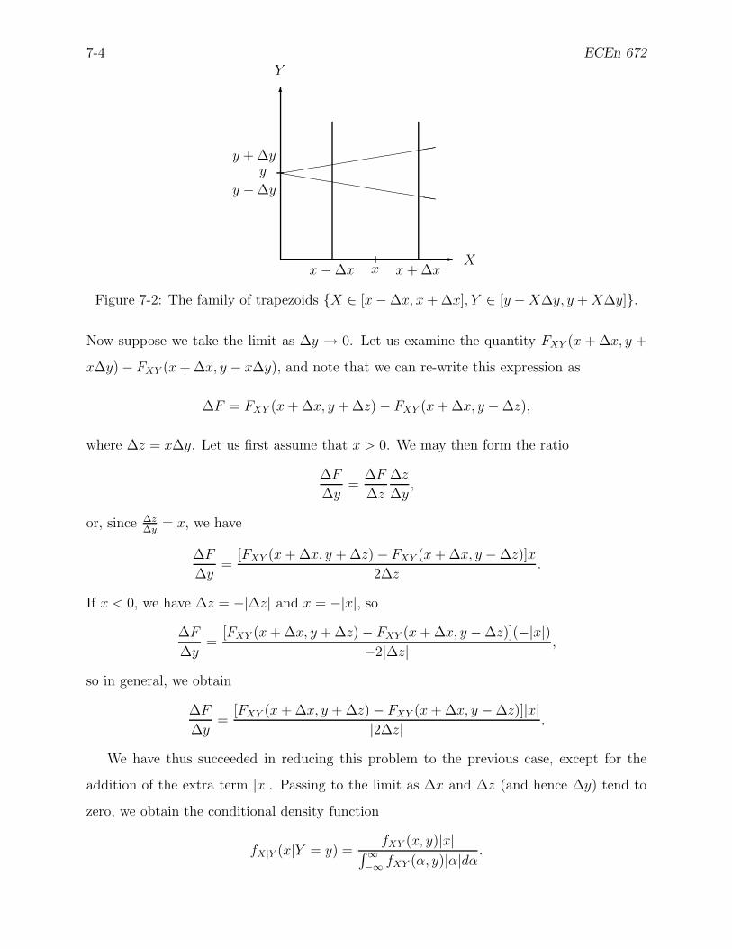
7-4 ECEn 672
-
6
X
Y
((((((((((((((
hhhhhhhhhhhhhh
x − ∆x x + ∆xx
y − ∆y
y + ∆yy
Figure 7-2: The family of trapezoids X ∈ [x − ∆x, x + ∆x], Y ∈ [y − X∆y, y + X∆y].
Now suppose we take the limit as ∆y → 0. Let us examine the quantity FXY (x + ∆x, y +
x∆y) − FXY (x + ∆x, y − x∆y), and note that we can re-write this expression as
∆F = FXY (x + ∆x, y + ∆z) − FXY (x + ∆x, y − ∆z),
where ∆z = x∆y. Let us first assume that x > 0. We may then form the ratio
∆F
∆y=
∆F
∆z
∆z
∆y,
or, since ∆z∆y
= x, we have
∆F
∆y=
[FXY (x + ∆x, y + ∆z) − FXY (x + ∆x, y − ∆z)]x
2∆z.
If x < 0, we have ∆z = −|∆z| and x = −|x|, so
∆F
∆y=
[FXY (x + ∆x, y + ∆z) − FXY (x + ∆x, y − ∆z)](−|x|)−2|∆z| ,
so in general, we obtain
∆F
∆y=
[FXY (x + ∆x, y + ∆z) − FXY (x + ∆x, y − ∆z)]|x||2∆z| .
We have thus succeeded in reducing this problem to the previous case, except for the
addition of the extra term |x|. Passing to the limit as ∆x and ∆z (and hence ∆y) tend to
zero, we obtain the conditional density function
fX|Y (x|Y = y) =fXY (x, y)|x|
∫∞−∞ fXY (α, y)|α|dα
.
Winter 2009 7-5
This is a very different conditional distribution than the one obtained with the rectangle
structure!
What’s going on here? We have competing definitions for the conditional density. This
is because there are many ways in which limiting operations can take place, and there is
no mathematical reason to prefer one over the other. This suggests that we must pay
very careful attention to the relationships between X and Y when computing conditional
expectations. This prompts us to ask a very significant question: Is there a way to define
the conditional expectation without first computing the conditional density function? To
answer this question, we need to discuss σ-fields.
7.2 σ-fields
Fundamental to all of probability theory is the concept of an event. An event is the outcome
of an experiment. For example, if I roll a die, the sure event is Ω = 1, 2, 3, 4, 5, 6, the null
event is the empty set, ∅, and some other examples of events are: “even and not 4” = 2, 6,“less than 5” = 1, 2, 3, 4, and “not 5” = 1, 2, 3, 4, 6. The power set, denoted 2Ω, is the
set of all subsets of Ω.
Probability theory involves the basic Boolean set operations of union, intersection, and
complementation. Any collection of sets that is closed under these operations is called a
field (if the collection of sets is finite, this collection is also called a Boolean algebra). For
example, consider the real line, <, and let A ⊂ < be any subset. The collection <, ∅, A, Acis a field, where Ac is the complement of A.
A sigma field (usually written σ-field) is a field that is closed under countable (not just
finite, but still enumerable) unions. Thus, formally, a σ-field F is a collection of sets (events)
such thatA ∈ F ⇒ Ac ∈ FA1, A2, . . . ,∈ F ⇒ ⋃∞
i=1 Ai ∈ F∅ ∈ F
Let Ω be a a sample space and let F be a σ-field defined over Ω. The pair Ω,F is called
a measurable space.
Examples such as coin-flips and dice-rolls are nice ways to introduce the concept of
events and fields, but we now need to move to a more sophisticated level, and discuss σ-
7-6 ECEn 672
fields in the context of random variables. Before doing so,however, we need to introduce
some new terminology. Let I be an arbitrary index set (countable or uncountable) and let
C = Aα, α ∈ I be an arbitrary collection of sets indexed by I. The σ-field generated by Cis the smallest σ-field that contains all of the members of C. In particular, suppose C is the
set of all open intervals on the real line. The σ-field generated by this collection is called
the Borel field. We will reserve the notation B for the Borel field. The Borel field has great
intuitive appeal, because it is the smallest σ-field that contains subsets of the real line that
we can describe with english sentences. It contains all singleton sets x, it contains all open
sets, all closed sets, all countable unions of such sets, their complements, intersections, and
so forth. Just about any subset of the real line that you can describe in a finite number of
words (and many that cannot be so easily described) is a member of the Borel field. As a
point of terminology, the elements of the Borel field are called Borel sets.
Let Ω,F be a measurable space, and consider a function X that maps a sample space
Ω to the real line; that is, X: Ω → <. We say that X is measurable with respect to F if,
and only if, the inverse images of all Borel sets in < are elements of F ; that is, if, and only if
A ∈ B ⇒ X−1(A) = ω ∈ Ω: X(ω) ∈ A ∈ F .
If a random variable is measurable with respect to a σ field F , we denote this fact by the
notation X ∈ F .14 Thus, a function is a random variable if and only if it is a measurable
function. We emphasize this point because, in general, a σ-field may be smaller than the
power set of the sample space. In particular, if the sample space is Ω = <, the real line, the
power set is huge, and not relevant to the experiment—every possible situation would be an
event. We need deal with σ-fields that are relevant to the experiment at hand, otherwise we
don’t have much chance of making meaningful interpretations.
Often, we will be dealing with more than one σ-field. Let F and G be two σ-fields. If
every element of F is also an element of G, we express this situation by the notation F ⊂ G.
Furthermore, if X is F -measurable, that is, X ∈ F , then X ∈ G.
14This is clearly an abuse of notation, because F is a collection of sets and X is a function, not a set.However, this, like many well-known abuses, are standard in the theory. Such abuses are cherished attributesof probability theory. I have often said that notation abuse is one of the distinguishing characteristics ofprobability theory—you get used to it.

Winter 2009 7-7
In most applications in signal detection and estimation, the σ fields of interest will be
generated by one or more random variables. Given a random variable Y , the σ-field generated
by Y , denoted σY , is defined as the smallest σ field with respect which Y is measurable,
that is, the smallest σ-field containing sets of the form
ω ∈ Ω: a < Y (ω) < b,
the inverse images under Y of open intervals.
By contrast, consider the smallest σ-field containing sets generated by the random vari-
able YX
, which contains sets of the form
ω ∈ Ω:a
X− c < Y (ω) <
a
X+ c
.
Furthermore, the σ-field generated by Y should be distinguished from the σ-field gener-
ated by the pair of random variables, (X, Y ), denoted σX, Y which is the smallest σ-field
containing sets of the form
ω ∈ Ω: , c < X < d, a < Y (ω) < b.
It is an important fact that if one σ-field is a subset of another, say
σY ⊂ σW,
then the random variable Y must be a function of the random variable W . We will not
prove this result, but refer the truly interested reader to [17, p. 12]. The converse is also
true, namely, if there exists a function f such that Y (ω) = f [W (ω)] then σY ⊂ σW.So, after the dust settles, what’s the big deal with σ-fields? In general, a σ-field is
a complete description of all of the possible events that can be detected as a result of
some experiment. In particular, the σ-field generated by a random variable is a complete
description of the events that can be detected as a result of observing the random variable or
any function of the random variable. Consider again the die-throwing problem. The sample
space is Ω = 1, 2, 3, 4, 5, 6, and let the function Y be defined as
Y (ω) =
1 if ω ∈ 2, 60 if ω ∈ 1, 3, 4−1 if ω = 5
.

7-8 ECEn 672
Recall that the σ-field generated by a function is the smallest σ-field that contains the inverse
images of all possible open sets on the real line. Let A be any open set in <. The inverse
image of Y is:
Y −1[A] =
2, 6 if 1 ∈ A & 0 6∈ A & − 1 6∈ A1, 2, 3, 4, 6 if 1 ∈ A & 0 ∈ A & − 1 6∈ A2, 5, 6 if 1 ∈ A & 0 6∈ A & − 1 ∈ A1, 3, 4 if 1 6∈ A & 0 ∈ A & − 1 6∈ A1, 3, 4, 5 if 1 6∈ A & 0 ∈ A & − 1 ∈ A5 if 1 6∈ A & 0 6∈ A & − 1 ∈ A1, 2, 3, 4, 5, 6 if 1 ∈ A & 0 ∈ A & − 1 ∈ A∅ if 1 6∈ A & 0 6∈ A & − 1 6∈ A
.
Since this collection of events is closed under complementation and union, it is the σ-field
generated by Y :
σY =
2, 61, 2, 3, 4, 62, 5, 61, 3, 41, 3, 4, 5
51, 2, 3, 4, 5, 6
∅
.
Now if we are given this σ-field, what events can be detected? The event “even and not 4” =
2, 6 is a member of σX, and so is the event “not 5” = 1, 2, 3, 4, 6, but the event
“less than 5” = 1, 2, 3, 4 is not in σY , and cannot be detected. In other words, no mat-
ter what value Y assumes, there is no way for me to ascertain that the event “less than 5”
occurred (although we can know whether or not the event “less than 5 but not 2” occurred).
Let X be a function given by
X(ω) =
1 if ω = 12 if ω = 23 if ω = 34 if ω = 45 if ω = 56 if ω = 6
.
For this problem, the σ-field generated by X is the power set of Ω. Now suppose Y is
observed. What can we say about X? In other words, what are the values you would expect
X to assume, given that you knew what values Y assumed? Clearly, this would be a function
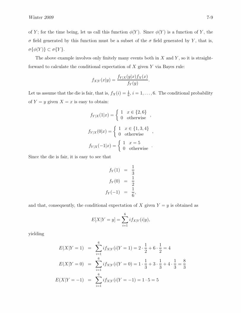
Winter 2009 7-9
of Y ; for the time being, let us call this function φ(Y ). Since φ(Y ) is a function of Y , the
σ field generated by this function must be a subset of the σ field generated by Y , that is,
σφ(Y ) ⊂ σY .The above example involves only finitely many events both in X and Y , so it is straight-
forward to calculate the conditional expectation of X given Y via Bayes rule:
fX|Y (x|y) =fY |X(y|x)fX(x)
fY (y).
Let us assume that the die is fair, that is, fX(i) = 16, i = 1, . . . , 6. The conditional probability
of Y = y given X = x is easy to obtain:
fY |X(1|x) =
1 x ∈ 2, 60 otherwise
,
fY |X(0|x) =
1 x ∈ 1, 3, 40 otherwise
,
fY |X(−1|x) =
1 x = 50 otherwise
.
Since the die is fair, it is easy to see that
fY (1) =1
3
fY (0) =1
2
fY (−1) =1
6,
and that, consequently, the conditional expectation of X given Y = y is obtained as
E[X|Y = y] =
6∑
i=1
ifX|Y (i|y),
yielding
E(X|Y = 1) =6∑
i=1
ifX|Y (i|Y = 1) = 2 · 1
2+ 6 · 1
2= 4
E(X|Y = 0) =
6∑
i=1
ifX|Y (i|Y = 0) = 1 · 1
3+ 3 · 1
3+ 4 · 1
3=
8
3
E(X|Y = −1) =
6∑
i=1
ifX|Y (i|Y = −1) = 1 · 5 = 5

7-10 ECEn 672
Calculations such as this are fine for situations involving probability mass functions,
because we don’t have to take limits. But, as we saw earlier, taking limits can be a prob-
lem. This motivates us to consider an alternative way to define conditional expectation—a
definition that does not require the specification of a conditional distribution function.
7.3 Conditioning on a σ-field
Given a random variable X satisfying the condition E|X| < ∞ (this condition can be relaxed
in various ways, but we don’t need to worry about that now), the conditional expectation of
X given the σ-field F = σY is defined as a random variable, written variously as EFX,
E[X|F ] or E[X|Y ], such that
1. E[X|F ] is an F -measurable function; that is, sets of the form
ω ∈ Ω: a < E[X|F ](ω) < b
are elements of F .
2. The random variable X − E[X|F ] is orthogonal15 to all F -measurable functions; that
is,
E[(X − E[X|F ])Z] = 0 ∀Z ∈ F .
This second property is the one that makes conditional expectations useful, and we will have
quite a bit to say about this as we progress through the course.
Viewed as a random variable (that is, a function of ω, the conditional expectation for the
six-sided die example is easily seen to be
E[X|Y ] =
4 ω ∈ 2, 683
ω ∈ 1, 3, 45ω = 5
Let’s pause a moment and examine some differences between this and the definition of
conditional expectation defined in terms of conditional distributions.
• The definition in terms of a conditional distribution is constructive, in that one is able
actually to compute the conditional expectation with the conditional distribution.
15Recall that orthogonality is defined in terms of the inner product of two random variables as 〈X, Y 〉 =E[XY ].
Winter 2009 7-11
• The definition in terms of σ-fields is not constructive. The definition is provided in
terms of properties that the conditional expectation must possess, but does not point
to a way to compute the conditional expectation.
This situation is somewhat similar, at least in spirit, to the situation with differential
equations. You may recall that, when considering equations of the form x = f(x, u),
all the theory provides is theorems regarding existence and uniqueness; it does not tell
us how to find the solution.
This is not to say, however, that the properties of conditional expectations cannot be
used to identify solutions—it just can’t generally be used to construct them. Take,
for example, the Wiener filter. Recall that orthogonality is the key property used to
identify the solution, But Wiener and Hopf had to be very creative to find a way to
solve the resulting equation.
Of course, if one can construct the conditional density or mass function, one certainly
may use it to compute the conditional expectation. But, by exploiting the properties
of conditional expectations, one may be able to develop ways to construct the condi-
tional expectation without first constructing the conditional density. Remember, the
conditional expectation is just the first moment of the conditional density, and one
may not need all of the information that the conditional density provides in order to
compute the conditional expectation. Sometimes we can obtain all of the information
we need by expoiting the properties of moments of distributions, rather than requiring
complete knowledge of the distribtuion.
• The conditional expectation defined in terms of a conditional distribution is, funda-
mentally a number; that is, it is computed for each value event Y = y. It may be
viewed as a function by computing it’s value for each possible value of y. With this
extension, we can think of conditional expectation as a function of Y , and thus as a
random variable.
• The conditional expectation defined in terms of a σ-field is, fundamentally, a random
variable. If that σ-field is generated by a random variable Y , then the conditional

7-12 ECEn 672
expectation is a function of Y , and can be evaluated for each event Y = y. With this
restriction, conditional expectation may be viewed as a number. (that is, it assumes
the value corresponding to the inverse image of the event Y = y).
Theoretically speaking, conditional expectations are generally more significant than con-
ditional densities (whose existence often requires stronger conditions). To show that con-
ditional expectations exist requires some deeper theory (specifically, the Radon-Nikodym
theorem) but for most applications it is enough to know the main properties of conditional
expectations, which are
1. If X ∈ F then E[X|F ] = X.
2. E[E[X|F ]] = EX.
3. If Z ∈ F then E[ZX|F ] = ZE[X|F ].
4. If F ⊂ G then E[X|F ] = E[E[X|F ]|G].
5. If F ⊂ G then E[X|F ] = E[E[X|G]|F ].
6. Jensen’s inequality: if f(·) is a convex function, then
E[f(X)|F ] ≥ f(E[X|F ]).
It is helpful in appreciating these properties to think of conditional expectation E[X|Y ]
as the projection of X onto the subspace generated by all functions of the random variable
Y , the projection being carried out via the inner product 〈X, Y 〉 = EXY .
When conditional densities exist, these properties can also be verified by elementary cal-
culations using Bayes’ rule. The important thing is that these properties also hold when
densities do not exist and the definition of conditional expectations has to be less construc-
tive. Essentially, what is done is to isolate certain important properties and then to define
the conditional expectation as a random variable that has those properties.
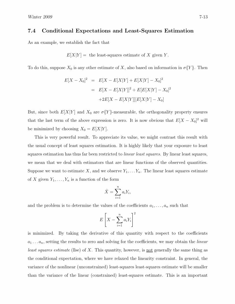
Winter 2009 7-13
7.4 Conditional Expectations and Least-Squares Estimation
As an example, we establish the fact that
E[X|Y ] = the least-squares estimate of X given Y .
To do this, suppose X0 is any other estimate of X, also based on information in σY . Then
E[X − X0]2 = E[X − E[X|Y ] + E[X|Y ] − X0]
2
= E[X − E[X|Y ]]2 + E[E[X|Y ] − X0]2
+2E[X − E[X|Y ]][E[X|Y ] − X0]
But, since both E[X|Y ] and X0 are σY -measurable, the orthogonality property ensures
that the last term of the above expression is zero. It is now obvious that E[X − X0]2 will
be minimized by choosing X0 = E[X|Y ].
This is very powerful result. To appreciate its value, we might contrast this result with
the usual concept of least squares estimation. It is highly likely that your exposure to least
squares estimation has thus far been restricted to linear least squares. By linear least squares,
we mean that we deal with estimators that are linear functions of the observed quantities.
Suppose we want to estimate X, and we observe Y1, . . . Yn. The linear least squares estimate
of X given Y1, . . . , Yn is a function of the form
X =n∑
i=1
aiYi,
and the problem is to determine the values of the coefficients a1, . . . , an such that
E
[
X −n∑
i=1
aiYi
]2
is minimized. By taking the derivative of this quantity with respect to the coefficients
a1 . . . an, setting the results to zero and solving for the coefficients, we may obtain the linear
least squares estimate (llse) of X. This quantity, however, is not generally the same thing as
the conditional expectation, where we have relaxed the linearity constraint. In general, the
variance of the nonlinear (unconstrained) least-squares least-squares estimate will be smaller
than the variance of the linear (constrained) least-squares estimate. This is an important

7-14 ECEn 672
result when linear estimates are not adequate. Perhaps even more importantly, however, the
fact that the conditional expectation is the least-squares estimate is an important theoretical
result that will guide our search for the construction of high-quality estimates.
To drive this point home, let’s compute the llse of X given Y for the six-sided die
problem discussed above. We first must compute the coefficient a that minimizes the quantity
E[X − aY ]2. Differentiating and equating the result to zero yields
a =E[XY ]
E[Y 2].
(This result is extremely important and will be seen many times throughout this course.)
The numerator of this expression is given by
E[XY ] =∑
x
∑
y
xyfXY (x, y) =∑
x
∑
y
xyfY |X(y|x)fX(x)
=1
6[2 + 6 − 5]
=1
2,
and the denominator is
E[Y 2] = 12 · 1
3+ 02 · 1
2+ (−1)2 · 1
6=
1
2.
Thus we have a = 1, and the linear least squares estimate of X given Y is
Xllse = Y,
or
Xllse =
1 if Y = 10 if Y = 0
−1 if Y = −1
Compare this with the unconstrained least-squares estimate of X given Y (namely, the
conditional expectation) and draw your own conclusion as to which is more reasonable!

Winter 2009 8-1
8 Bayes Estimation Theory
Suppose you are to observe a random variable X, whose distribution depends on a parameter
θ. The maximum likelihood approach to estimation says that you should take as your
estimate of an unknown parameter that value that is the most likely, out of all possible
values of the parameter, to have given rise to the observed data. Before observations are
taken, therefore, the maximum likelihood method is silent as to any predictions it would
make about either the value of the parameter or the values future observations would take.
Rather, the attitude of a rabid “max-like” enthusiast would be: “Wait until all of the data
are collected, give them to me, be patient, and soon I will give you an estimate of what the
values of the parameters were that generated the data.” If you were to ask him for his best
guess, before you collected the data, as to what values would be assumed by either the data
or the parameters, his response would simply be: “Don’t be ridiculous.”
On the other hand, a Bayesian would be all too happy to give you estimates, both
before and after the data have been obtained. Before the observation, she would give you,
perhaps, the mean value of the a priori distribution of the parameter, and after the data were
collected she would give you the mean value of the a posteriori distribution of the parameter.
She would offer, as predicted values of the observations, the mean value of the conditional
distribution of X given the expected value of θ (based on the a priori distribution).
Some insight may be gained into how the prior distribution enters into the problem of
estimation through the following example.
Example 8-1 Let X1, . . . , Xm denote a random sample of size m from the normal distri-
bution N (θ, σ2). Suppose σ is known, and we wish to estimate θ. We are given the prior
density θ ∼ N (ϑ0, σ2θ), that is,
fθ(ϑ) =1√
2πσθ
exp
[
−(ϑ − ϑ0)2
2σ2θ
]
.
Before getting involved in deep Bayesian principles, let’s just think about ways we could use
this prior information.
1. We could consider computing the maximum likelihood estimate of θ (which we saw
earlier is just the sample average) and then simply averaging this result with the mean
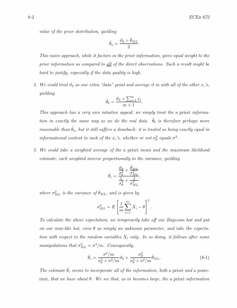
8-2 ECEn 672
value of the prior distribution, yielding
θa =ϑ0 + θML
2.
This naive approach, while it factors in the prior information, gives equal weight to the
prior information as compared to all of the direct observations. Such a result might be
hard to justify, especially if the data quality is high.
2. We could treat ϑ0 as one extra “data” point and average it in with all of the other xi’s,
yielding
θb =ϑ0 +
∑mi=1 xi
m + 1.
This approach has a very nice intuitive appeal; we simply treat the a priori informa-
tion in exactly the same way as we do the real data. θb is therefore perhaps more
reasonable than θa, but it still suffers a drawback: it is treated as being exactly equal in
informational content to each of the xi’s, whether or not σ2θ equals σ2.
3. We could take a weighted average of the a priori mean and the maximum likelihood
estimate, each weighted inverse proportionally to the variance, yielding
θc =
ϑ0
σ2θ
+ θML
σ2ML
1σ2
θ
+ 1σ2
ML
,
where σ2ML is the variance of θML, and is given by
σ2ML = E
[
1
m
m∑
i=1
Xi − θ
]2
.
To calculate the above expectation, we temporarily take off our Bayesian hat and put
on our max-like hat, view θ as simply an unknown parameter, and take the expecta-
tion with respect to the random variables Xi only. In so doing, it follows after some
manipulations that σ2ML = σ2/m. Consequently,
θc =σ2/m
σ2θ + σ2/m
ϑ0 +σ2
θ
σ2θ + σ2/m
θML. (8-1)
The estimate θc seems to incorporate all of the information, both a priori and a poste-
riori, that we have about θ. We see that, as m becomes large, the a priori information
Winter 2009 8-3
is forgotten, and the maximum likelihood portion of the estimator dominates. We also
see that if σ2θ << σ2, then the a priori information tends to dominate.
The estimate provided by θc appears to be, of the three we have presented, the one most
worthy of our attention. We shall eventually see that it is indeed a Bayesian estimate.
8.1 Bayes Risk
The starting point for Bayesian estimation, as it was for Bayesian detection, is the specifi-
cation of a loss function and the calculation of the Bayes risk. Recall that the cost function
is a function of the state of nature and the decision function, that is, it is of the general
form L[θ, φ(X)]. For our development, we will restrict the structure of the loss function to
be function of the difference, that is, to be of the form L[θ − φ(X)]. Although this restricts
us to only a small subset of all possible loss functions, we will see that it still leads us to
some very interesting and useful results. We will examine three different cost functionals:
(a) squared error, (b) absolute value of error, and (c) uniform cost. Of these, the squared
error criterion will emerge as being the most important and deserving of study.
We saw earlier (see (5-24)) that, under appropriate regularity conditions, we may reverse
the order of integration in the calculation of the Bayes risk function to obtain
r(τ, φ) =
∫
X
∫
Θ
L[ϑ, φ(x)]fθ|X(ϑ | x)dϑ
fX(x)dx,
and noted that we could minimize the Bayes risk by minimizing the inner integral for each
x separately; that is, we may find, for each x, the action, call it φ(x), that minimizes
∫
L[ϑ, φ(x)]fθ|X(ϑ | x)dϑ.
In other words, the Bayes decision rule minimizes the posterior conditional expected loss,
given the observations.
Let us now examine the structure of the Bayes rule under the three cost functionals we
have defined.
Squared Error Loss
Let us first consider squared error loss, and introduce the concept via the following
example.

8-4 ECEn 672
Example 8-2 Consider the estimation problem in which Θ = ∆ = (0,∞) and L(θ, δ) =
(θ−δ)2. Suppose we observe the value of a random variable X having a uniform distribution
on the interval (0, θ) with density
fX|θ(x | ϑ) =
1/ϑ if 0 < x < ϑ
0 otherwise.
Note that we may write
fX|θ(x | ϑ) =1
ϑI(0,ϑ)(x) =
1
ϑI(x,∞)(ϑ).
We are to find a Bayes rule with respect to the prior distribution Fθ with density
fθ(ϑ) =
ϑe−ϑ if ϑ > 0
0 otherwise.
The joint density of X and θ is, therefore,
fXθ(x, ϑ) = fX|θ(x | ϑ)fθ(ϑ) =1
(ϑIx,∞)ϑe−ϑ,
and the marginal distribution of X has the density
fX(x) =
∫ ∞
−∞fXθ(x, ϑ)dϑ =
e−x if x > 0
0 otherwise.
Hence, the posterior distribution of θ, given X = x, has the density
fθ|X(ϑ | x) =fXθ(x, ϑ)
fX(x)=
ex−ϑ if ϑ > x
0 otherwise,
where x > 0. The posterior expected loss, given X = x, is
EL(θ, δ |X = x) = ex
∫ ∞
x
(ϑ − δ)2e−ϑdϑ.
To find the δ that minimizes this expected loss, we may set the derivative with respect to δ
to zero:d
dδEL(θ, δ |X = x) = −2ex
∫ ∞
x
(ϑ − δ)e−ϑdϑ = 0.
This implies
φ(x) = δ =
∫∞x
ϑe−ϑdϑ∫∞
xe−ϑdϑ
=(x + 1)e−x
e−x= x + 1.
This, therefore, is a Bayes decision rule with respect to Fθ: if X = x is observed, then the
estimate of θ is x + 1.

Winter 2009 8-5
The problem of point estimation of a real parameter, using quadratic loss, occurs so
frequently in engineering applications that it is worthwhile to make the following observation.
The posterior expected loss, given X = x, for a quadratic loss function at δ is the second
moment about δ of the posterior distribution of θ given x. That is,
EL(θ, δ |X = x) =
∫ ∞
−∞(ϑ − δ)2fθ|X(ϑ | x)dϑ.
Exercise 8-1 Show that
EL(θ, δ |X = x) =
∫ ∞
−∞(ϑ − δ)2fθ|X(ϑ | x)dϑ
is minimized by taking δ as the mean of the posterior distribution, that is,
φ(x) = δ = E(θ |X = x).
This result is important enough to state as a general rule:
Rule. In the problem of estimating a real parameter θ with quadratic loss, a Bayes decision
rule with respect to a given prior distribution for θ is the mean of the posterior distribution
of θ, given the observations. The resulting estimate is termed the mean square estimate of
θ, and is denoted θMS.
Absolute Error Loss
Another important loss function is absolute value of the difference, L(θ, δ) = |θ− δ|. The
Bayes risk is minimized by minimizing
EL(θ, δ |X = x) =
∫ ∞
−∞|ϑ − δ|fθ|X(ϑ | x)dϑ.
Exercise 8-2 Show that
EL(θ, δ |X = x) =
∫ ∞
−∞|ϑ − δ|fθ|X(ϑ | x)dϑ
is minimized by taking
φ(x) = δ = median fθ|X(ϑ | x),
that is, Bayes rule corresponding to the absolute error criterion is to take δ as the median
of the posterior distribution of θ, given X = x.
8-6 ECEn 672
This result is also important enough to state as a general rule:
Rule. In the problem of estimating a real parameter θ with absolute error loss, a Bayes
decision rule with respect to a given prior distribution for θ is the median of the posterior
distribution of θ, given the observations. The resulting estimate is termed the absolute error
estimate of θ, and is denoted θABS .
Uniform Cost
The loss function associated with uniform cost is defined as
L(ϑ, δ) =
0 if |ϑ − δ| ≤ ε/2
1 if |ϑ − δ| > ε/2..
In other words, an error less than ε/2 is as good as no error, and if the error is greater than
ε/2, we assign a uniform cost. The Bayes risk is minimized by minimizing
∫ ∞
−∞L(ϑ, δ)fθ|X(ϑ | x)dϑ =
∫ δ−ε/2
−∞fθ|X(ϑ | x)dϑ +
∫ ∞
δ+ε/2
fθ|X(ϑ | x)dϑ
= 1 −∫ δ+ε/2
δ−ε/2
fθ|X(ϑ | x)dϑ.
Consequently, the Bayes risk is minimized when the integral
∫ δ+ε/2
δ−ε/2
fθ|X(ϑ | x)dϑ.
is maximized.
Exercise 8-3 Show that∫ δ+ε/2
δ−ε/2
fθ|X(ϑ | x)dϑ
is maximized when ϑ is the midpoint of what me might call the modal interval of length ε.
Define “modal interval of length ε” so that this makes sense, and state a rule for finding
Bayes rules, using this loss function.
8.2 MAP Estimates
Of particular interest with the uniform cost function is the case in which ε is arbitrarily small
but nonzero. In this case, it is evident that this integral is maximized when ϑ assumes the
value at which the posterior density fθ|X(ϑ | x) is maximized.

Winter 2009 8-7
Definition. The mode of a distribution is that value that maximizes the probability density
function.
Definition. The value of ϑ that maximizes the a posteriori density (that is, the mode of the
posterior density) is called the maximum a posteriori probability (MAP) estimate of θ.
If the posterior density of θ given X is unimodal and symmetric, then it is easy to see
that the MAP estimate and the mean square estimate coincide, for then the posterior density
attains its maximum value at its expectation. Furthermore, under these circumstances, the
median also coincides with the mode and the expectation. Thus, if we are lucky enough to
be dealing with such distributions, the various estimates all tend to the same thing.
Although we eschewed, in the development of maximum likelihood estimation theory,
the characterization of θ as being random, we may gain some valuable understanding of
the maximum likelihood estimate by considering θ to be a random variable whose prior
distribution is so dispersed (that is, has such a large variance) that the information provided
by the prior is vanishingly small. If the theory is consistent, we would have a right to
expect that the maximum likelihood estimate would be the limiting case of such a Bayesian
estimate.
Let θ be considered as a random variable distributed according to the a priori density
fθ(ϑ). The a posteriori distribution for θ, then, is given by
fθ|X(ϑ | x) =fX|θ(x | ϑ)fθ(ϑ)
fX(x). (8-2)
If the logarithm of the a posteriori density is differentiable with respect to θ, then the
MAP estimate is given by the solution to
∂ log fθ|X(ϑ | x)
∂ϑ
∣∣∣∣ϑ=θMAP
= 0. (8-3)
This equation is called the MAP equation.
Taking the logarithm of (8-2) yields
log fθ|X(ϑ | x) = log fX|θ(x | ϑ) + log fθ(ϑ) − log fX(x),
and since fX(x) is not a function of θ, the MAP equation becomes
∂ log fθ|X(ϑ | x)
∂ϑ=
∂ log fX|θ(x | ϑ)
∂ϑ+
∂ log fθ(ϑ)
∂ϑ. (8-4)
8-8 ECEn 672
Comparing (8-4) to the standard maximum likelihood equation
∂L(θ, x)
∂θ
∣∣∣∣θ=θML
= 0,
we see that the two expressions differ by ∂ log fθ(ϑ)∂ϑ
. If fθ(ϑ) is sufficiently “flat,” (that is, if
the variance is very large) its logarithm will also be flat, so the gradient of the logarithm
will be nearly zero, and the a posteriori density will be maximized, in the limiting case, at
the maximum likelihood estimate.
Example 8-3 Let X1, . . . , Xm denote a random sample of size m from the normal distribu-
tion N (θ, σ2). Suppose σ is known, and we wish to find the MAP estimate for the mean, θ.
The joint density function for X1, . . . , Xm is
fX1,...,Xm(x1, . . . , xm | θ) =
m∏
i=1
1√2πσ
exp
[
−(xi − ϑ)2
2σ2
]
,
Suppose θ is distributed N (0, σ2θ), that is,
fθ(ϑ) =1√
2πσθ
exp
[
− ϑ2
2σ2θ
]
.
Straightforward manipulation yields
∂ log fθ|X(ϑ | x)
∂ϑ=
1
σ2
m∑
i=1
(xi − ϑ) − ϑ
σ2θ
.
Equating this expression to zero and solving for ϑ yields
θMAP =σ2
θ
σ2θ + σ2
m
1
m
m∑
i=1
xi.
Now, it is clear that as σ2θ → ∞, the limiting expression is the maximum likelihood estimate
θML. It is also true that, as m → ∞, the MAP estimate asymptotically approaches the ML
estimate. Thus, as the knowledge about θ from the prior distribution tends to zero, or as
the amount of data becomes overwhelming, the MAP estimate converges to the maximum
likelihood estimate.
Winter 2009 8-9
8.3 Conjugate Prior Distributions
In general, the marginal density fX(x) and the posterior density fθ|X(ϑ | x) are not easily
calculated. We are interested in establishing conditions on the structure of the distributions
involved that ensure tractability in the calculation of the posterior distribution.
Definition. Let F denote a class of conditional density functions fX|θ, indexed by ϑ as ϑ
ranges over all the values in Θ. A class P of distributions is said to be a conjugate family
for F if fθ|X ∈ P for all fX|θ ∈ F and all fθ ∈ P. In other words, a family of distributions
is a conjugate family if it contains both the prior and the posterior density for all possible
conditional densities. A conjugate family is said to be closed under sampling.
A significant part of the Bayesian literature has been devoted to finding conjugate fami-
lies. We give some examples of conjugate families, stated without proof (for proofs, see [2]),
except for the most important conjugate family, at least insofar as engineering is concerned:
the normal distribution.
Example 8-4 Suppose that X1, . . . , Xm is a random sample from a Bernoulli distribution
with parameter 0 ≤ θ ≤ 1 with density
fX|θ(x | ϑ) =
ϑx(1 − ϑ)1−x x ∈ 0, 10 otherwise
.
Suppose also that the prior distribution of θ is a beta distribution with parameters α > 0 and
β > 0, with density
fθ(ϑ) =
Γ(α+β)Γ(α)Γ(β)
ϑα−1(1 − ϑ)β−1 0 < ϑ < 1
0 otherwise.
Then the posterior distribution of θ when Xi = xi, i = 1, . . . , m is a beta distribution with
parameters α + y and β + m − y where y =∑m
i=1 xi.
Example 8-5 Suppose that X1, . . . , Xm is a random sample from a Poisson distribution
with parameter θ > 0 with density
fX|θ(x | ϑ) =
e−ϑϑx
x!x = 0, 1, 2, . . .
0 otherwise.

8-10 ECEn 672
Suppose also that the prior distribution of θ is a gamma distribution with parameters α > 0
and β > 0, with density
fθ(ϑ) =
βα
Γ(α)ϑα−1eβϑ ϑ > 0
0 otherwise.
Then the posterior distribution of θ when Xi = xi, i = 1, . . . , m is a gamma distribution with
parameters α + y and β + m where y =∑m
i=1 xi.
Example 8-6 Suppose that X1, . . . , Xm is a random sample from an exponential distribution
with parameter θ > 0 with density
fX|θ(x | ϑ) =
θe−θx x > 0
0 otherwise.
Suppose also that the prior distribution of θ is a gamma distribution with parameters α > 0
and β > 0, with density
fθ(ϑ) =
βα
Γ(α)ϑα−1eβϑ ϑ > 0
0 otherwise.
Then the posterior distribution of θ when Xi = xi, i = 1, . . . , m is a gamma distribution with
parameters α + m and β + y where y =∑m
i=1 xi.
Example 8-7 Suppose that X1, . . . , Xm is a random sample from a normal distribution with
unknown mean θ and known variance σ2. Suppose also that the prior distribution of θ is a
normal distribution with mean ϑ0 and variance σ2θ . Then the posterior distribution of θ when
Xi = xi, i = 1, . . . , m is a normal distribution with mean
θc =
ϑ0
σ2θ
+ xσ2
m
1σ2
θ
+ 1σ2
m
(8-5)
and variance
σ2θ
=σ2
mσ2θ
σ2m + σ2
θ
, (8-6)
where
x =1
m
m∑
i=1
xi and σ2m = σ2/m.

Winter 2009 8-11
Due to its importance, we provide a demonstration of the above claim. For −∞ < ϑ < ∞,
the conditional density of X1, . . . , Xm satisfies
fX1...Xm|θ(x1, . . . , xm | ϑ) =m∏
i=1
1√2πσ
exp
[
−(xi − ϑ)2
2σ2
]
= (2π)−m2 σ−m exp
[
− 1
2σ2
m∑
i=1
(xi − x)2
]
exp
[−m
2σ2(ϑ − x)2
]
.(8-7)
The prior density of θ satisfies
fθ(ϑ) =1√
2πσθ
exp
[
−(ϑ − ϑ0)2
2σ2θ
]
, (8-8)
and the posterior density function of θ will be proportional to the product of (8-7) and (8-8).
Letting the symbol ∝ denote proportionality, we have
fθ|X1,...,Xm(ϑ | x1, . . . , xm) ∝ exp
[−m
2σ2(ϑ − x)2
]
exp
[
−(ϑ − ϑ0)2
2σ2θ
]
= exp
[
−(ϑ − x)2
2σ2m
− (ϑ − ϑ0)2
2σ2θ
]
.
Simplifying the exponent, we obtain
(ϑ − x)2
σ2m
+(ϑ − ϑ0)
2
σ2θ
=σ2
m + σ2θ
σ2mσ2
θ
(ϑ − θc)2 +
1
σ2m + σ2
θ
(x − ϑ0)2,
where θc is given by (8-5). Thus,
fθ|X1,...,Xm(ϑ | x1, . . . , xm) ∝ exp
[
−1/2σ2
m + σ2θ
σ2mσ2
θ
(ϑ − θc)2
]
.
Consequently, suitably normalized, we see that the posterior density of θ given X1, . . . , Xm
is normal with mean given by (8-5) and variance given by (8-6). 2
Upon rearranging (8-5) we see that
θc =σ2
m
σ2θ + σ2
m
ϑ0 +σ2
θ
σ2θ + σ2
m
x,
which is exactly the same as the estimate given by (8-1). Thus, the weighted average, as
proposed as a reasonable way to incorporate prior information into the estimate, turns out to
be exactly a Bayes estimate for the parameter given that the prior is a member of the normal
conjugate family.
8-12 ECEn 672
8.4 Improper Prior Distributions
As we saw with the example developed for the MAP estimate, sometimes the prior knowledge
available about a parameter is very slight when compared to the information we expect to
acquire from observations. Consequently, it may not be worthwhile for us to spend a great
deal of time and effort in determining a specific prior distribution. Rather, it might be
useful in some circumstances to make use of a standard prior that would be suitable in many
situations for which it is desirable to represent vague or uncertain prior information.
Definition. A proper density function is one whose integral over the parameter space is unity.
This is the only type of density function with which we have had anything to do with thus
far. In fact, we know that virtually any continuous, nonnegative function whose integral
over the parameter space is finite can be turned into a proper density function by dividing
it by the integral.
Definition. An improper density function is a nonnegative function whose integral over the
whole parameter space Θ is infinite.
For example, if Θ is the real line and, because of vagueness, the prior distribution of
θ is smooth and very widely spread out over the line, then we might find it convenient to
assume a uniform, or constant density over the whole line in order to represent this prior
information. Even though this is not a proper density, we might consider formally carrying
out the calculations of Bayes theorem and attempt to compute a posterior distribution.
Suppose Θ = (−∞,∞), let fθ(ϑ) = 1 be an improper prior for θ, and suppose X = x is
observed. Formally applying Bayes theorem, we obtain
fθ|X(ϑ | x) =fX|θ(x | ϑ)fθ(ϑ).
∫
ΘfX|θ(x | ϑ′)fθ(ϑ′)dϑ′ =
fX|θ(x | ϑ)∫
ΘfX|θ(x | ϑ′)dϑ′ .
We see that, if∫
Θ
fX|θ(x | ϑ)dϑ < ∞, (8-9)
then the posterior density fθ|X(ϑ | x) is at least defined.
Example 8-8 Suppose X1, . . . , Xm are samples from a normal population with mean θ and
variance σ2. Let θ be distributed according to an improper prior fθ(ϑ) = 1. The conditional
Winter 2009 8-13
density of X1, . . . , Xm given θ = ϑ is
fX1...Xm|θ(x1, . . . , xm | ϑ) =
m∏
i=1
1√2πσ
exp
[
−(xi − ϑ)2
2σ2
]
= (2π)−m2 σ−m exp
[
− 1
2σ2
m∑
i=1
(xi − x)2
]
exp
[−m
2σ2(ϑ − x)2
]
,
where x = 1m
∑mi=1 xi. The first exponential term in this expression is independent of ϑ, and
since the integral of the entire expression quantity with respect to ϑ over (−∞, ∞) is finite,
we may normalize this quantity to obtain a posterior density for θ of the form
fθ|X1...Xm(ϑ | x1, . . . , xm) =1√
2πσm
exp
[
−(ϑ − x)2
2σ2m
]
,
where σm = σ/√
m. Thus, the posterior distribution of θ when Xi = xi, i = 1, . . . , m, is
a normal distribution with mean x and variance σ2/m. Although the prior distribution is
improper, the posterior distribution is a proper normal distribution after just one observation
has been made. Under squared error loss, therefore, the “Bayes estimate” for θ, using an
improper prior, is the sample mean. Comparing this with previous results, we see that this
estimate also coincides with the maximum likelihood estimate. Consequently, we may view
the maximum likelihood as (a) the limit of a MAP estimate as the variance of the prior
distribution tends to infinity, or (b) the mean square estimate associated with an improper
prior distribution.
8.5 Sequential Bayes Estimation
Thus far in our treatment of estimation, we have assumed that all of the information to
be used to make a decision or estimate is available at one time. More generally, we are
interested in addressing problems where the data becomes available as a function of time,
that is, sequentially. To introduce this topic, we will consider first the case of estimating θ
given two measurements, obtained at different times.
Let θ be the parameter to be estimated, and suppose X1 and X2 are two observed
random variables. Suppose that X1 and X2 have a joint conditional probability density
function fX1X2|θ(x1, x2 | ϑ), for each ϑ ∈ Θ. The posterior density function of θ conditioned

8-14 ECEn 672
on X1 = x1 and X2 = x2 is
fθ|X1X2(ϑ | x1, x2) =fX1X2|θ(x1, x2 | ϑ)fθ(ϑ)
∫
ΘfX1X2|θ(x1, x2 | ϑ′)fθ(ϑ′)dϑ′ . (8-10)
If we had both X1 and X2 at our disposal, then we would simply use this posterior density
to form our estimate according to the loss function we choose, say, for example, squared
error loss. But suppose we first observe X1, and at some future time have the prospect of
observing X2. There are two ways we might proceed: (a) we could put X1 on the shelf
and wait until X2 is obtained to calculate our estimate; (b) we could use X1 as soon as it
is obtained to estimate θ using that information only, then update that estimate once X2
becomes available. Our goal is to show that these two approaches yield the same result.
We first compute the posterior distribution of θ given X1 only:
fθ|X1(ϑ | x1) =fX1|θ(x1 | ϑ)fθ(ϑ)
∫
ΘfX1|θ(x1 | ϑ′)fθ(ϑ′)dϑ′ . (8-11)
We next compute the conditional distribution of X2 given θ = ϑ and X1 = x1, yielding
fX2|θX1(x2 | ϑ, x1) =
fX1X2|θ(x1, x2 | ϑ)
fX1|θ(x1 | ϑ), (8-12)
and compute the corresponding posterior density of θ:
f ′θ|X1X2
(ϑ | x1, x2) =fX2|θX1(x2 | ϑ, x1)fθ|X1(ϑ | x1)
∫
ΘfX2|θX1
(x2 | ϑ′, x1)fθ|X1(ϑ′ | x1)dϑ′ (8-13)
Substituting (8-11) and (8-12) into (8-13) yields, after some simplification, the conditional
density given in (8-10), thus we see that if the observations are received sequentially, the
posterior distribution can also be computed sequentially, that is,
f ′θ|X1X2
(ϑ | x1, x2) = fθ|X1X2(ϑ | x1, x2).
It also follows from this derivation that if the posterior distribution of θ when X1 = x1 and
X2 = x2 is computed in two stages, the final result is the same regardless of whether X1 or
X2 is observed first.
Exercise 8-4 Show that substituting (8-11) and (8-12) into (8-13) yields (8-10).

Winter 2009 8-15
It is straightforward to generalize this result to the case of observing X1, X2, X3, . . . ,
and sequentially updating the estimate of θ as time progresses. There is a general theory
of sequential sampling, which we will not develop in this class, that treats this problem in
detail. For details, see [2, 3]. Although we will not pursue sequential detection theory further
in this course, we will develop the concept of a closely related subject, that of sequential
estimation theory.
9-16 ECEn 672
9 Linear Estimation Theory
9.1 Introduction
The concept of least squares is probably the oldest of all mathematically based estimation
techniques. The history begins with Gauss. As the story goes, in 1801 an Italian astronomer
named Piazzi discovered a new planet (actually an asteroid), named Ceres, and begin plotting
its path against the fixed stars. His work was interrupted, however, and when he returned
to it he was unable to relocate the new object. The problem came to the attention of
Gauss, who wondered if there was some way to predict the location of the object form
the scanty data available. To address this problem, he took the few data points at his
disposal, and devised a way to “fit” an orbital model to them. His brilliance and intuition
led him to compute the values of the observations as a function of the orbital model, and
then adjust the model parameters to minimize the square of the difference between these
values and the actual observations. Needless to say, his scheme was successful, thus giving us
another reason to admire and respect this giant of mathematics. Although this application
of least squares is perhaps the most famous one, Gauss was not the only one to discover
it (his experience just makes the best story). He claims to have discovered the technique
in 1795, but the technique was also discovered independently in that same time frame by
Legendre, in France, and by Robert Adrian, in the United States. Also, there is evidence
that the German-Swiss physicist Johann Heinrich Lambert (1728–1777) discovered and used
the method of least squares before Gauss was born. This is another example of Hutching’s
Rule: “Originality usually dissolves upon inspection16.” So if you think you are the first to
discover something, it may only be a matter of time before others lay claim to having gotten
there first (of course, you still may get the credit).
A major motivation for the additional attention to least squares and related ideas is
due to the space program that began in earnest in the 1950’s. This program developed the
requirement to track satellites, predict orbital trajectories, etc. The major successes in this
development are due to Kalman [9], Stratonovich [14], (Russian), and Swerling [15]. These
methods are based upon the so-called Riccati equation—other approaches are possible, the
16After Brad Hutchings.

Winter 2009 9-17
most notable of which are the so-called square-root method and the Chandrasekhar method.
We will not spend much time on non-Riccati methods, but you should know that the square-
root method leads to perhaps the most stable (numerically) of ways to implement the Kalman
filter.
Example 9-9 (Curve fitting). One way to apply least squares is as a method of fitting
a curve to a given set of data. For example, suppose data pairs (x1, y1), . . . , (xm, ym) are
observed, and we suspect, for physical reasons, that these values should correspond to the
curve generated by the function y = g(x). We may attribute deviations from this equation to
measurement errors or some unmodeled phenomenon such as disturbances. If the function g
is parameterized by some quantity θ, then we would write y = g(x; θ), and a natural course
of action (provided we are endowed with some of Gauss’s insight) would be to determine that
value, θ, such that the squared error of the deviation from the proposed curve is minimized.
That is, we want to minimize the loss function
L(θ) =
m∑
i=1
(yi − g(xi; θ))2. (9-14)
The estimate, θ, is called the least squares estimate of θ.
To be specific, suppose xi = Ii represents the input current to a resistor at time i,, and
yi = Vi represents the voltage drop across the resistor. Let θ = R, the resistance of the
device. Since measurement errors may occur when measuring both the voltage and current,
we would not expect that all (or even any) of the observational pairs (xi, yi) would lie exactly
on the line V = RI, even if R were precisely known and Ohm’s law were exactly obeyed to
arbitrary precision. If we compute the least squares estimate of R, then (9-14) becomes
L(R) =
m∑
i=1
(Vi − RIi)2.
We may obtain the global minimum of this function by differentiating with respect to R,
setting the result to zero, and solving for the corresponding value of the resistance, denoted
R:
R =
∑mi=1 ViIi∑m
i=1 I2i
.
9-18 ECEn 672
Although the method of least squares does not, strictly speaking, require any appeal to
probability or statistics, the modern developments of this theory are almost always couched
in a probabilistic framework. In our development, we will follow the probabilistic frame-
work, and view the pairs (xi, yi) as samples from the population (X, Y ) where X and Y are
random variables with known joint distribution, and perform the minimization in terms of
the expected loss.
9.2 Minimum Mean Square Estimation (MMSE)
Suppose we have two real random variables X, Y , with a known joint density function
fXY (x, y), and assume Y is observed (measured). What can be said about the value X
takes? In other words, we wish to estimate X given that Y = y. To be specific, we desire to
invoke an estimation rule
X = h(Y ),
where the random variable X is an estimate of X. The mapping h : < 7→ < is some function
only of Y . Thus, given Y = y, we will assign the value
x = h(y)
to the estimate of X.
Let us define the estimation error as
X = X − X,
the difference between the true (but unknown value of X) and the estimate, X. Ideally, we
would like X ≡ 0, but this is usually too much to hope for, since X is not generally a 1-1
function of Y . So the best we can obtain is to choose h(·) such that X is “small” in average
value. Precisely, let L : < 7→ [0, ∞) be some nonnegative functional of X. Then we will
attempt to choose the estimator Some candidates:
• L(X) = E|X| (absolute value) weights all errors equally;
• L(X) = E|X|2 (squared error) weights small errors less than large ones;
Winter 2009 9-19
• L(X) =
0 if |X| ≤ ε
K if |X| > εwhere K and ε are some positive quantities;
• Lots of other rather arbitrary error functions.
A Remarkable fact: the squared error function is the one deserving of the most study.
1. The mean-square estimate can be interpreted as a conditional expectation: X =
E(X|Y = y), where E denotes mathematical expectation.
2. For Gaussian random variables the mean-square estimate is a linear function of the
observables, leading to easy computations.
3. Sub-optimum estimates are easy to obtain (only first and second moments are required–
mean and covariance).
4. Stochastic linear mean-squares theory has many illuminating connections with control
theory, including Riccati equations, Matrix inversions, and Observers.
5. There are also connections with martingale theory, likelihood ratios, and nonlinear
estimation.
9.3 Estimation Given a Single Random Variable
The general problem is to observe one set of random variables and then infer the value of other
random variables. This procedure generally requires knowledge of the joint distributions of
all random variables. But we will see how to get something without all of this knowledge.
We will assume a linear relationship among random variables and will employ the mean-
square error criterion. Then knowledge of the joint pdf can be replaced by knowledge of only
the first and second order statistics.
Let X and Y be two zero-mean real random variables. Suppose we wish to find an
estimator of the form
X = hY
where h is a constant chosen such E(X − X)2 is minimized. (Thus, the function h(Y ) = hY
is linear.)

9-20 ECEn 672
To solve this problem, we expand the cost functional to obtain
L = E(X − X)2 = E(X − hY )2 = EX2 − 2hEXY + h2EY 2
and set the derivative with respect to h to zero and solve for the resulting value of h:
∂L
∂h= 2hEY 2 − 2EXY = 0
or
h =EXY
EY 2.
(The structure of h is significant: it is the ratio of the cross-correlation of X and Y and the
auto-correlation of Y . This structure permeates much of estimation theory.) Thus,
X = EXY (EY 2)−1Y (9-15)
and the minimum mean-square error is
E(X − X)2 = EX2 − 2EXY
EY 2EXY +
(EXY )2
(EY 2)2EY 2 = EX2 − (EXY )2
EY 2.
9.4 Estimation Given two Random Variables
Suppose we have two measurements Y1 and Y2; Find X. We must look for an estimator that
is a linear combination of the observations Y1 and Y2, that is, has the form
X = h1Y1 + h2Y2
where h1, h2 are chosen to to minimize the expected squared error.
To solve this problem, observe that we have
L = E(X − h1Y1 − h2Y2)2
= EX2 + h21EY 2
2 + h22EY 2
2 − 2h1EXY1 − 2h2EXY2 + 2h1h2EY1Y2.
Differentiating with respect to h1 and h2 and equating to zero yields
EXY1 = h1EY 21 + h2EY1Y2
EXY2 = h2EY 22 + h1EY1Y2
Winter 2009 9-21
which, in matrix form, is
[EXY1 EXY2] = [h1 h2]
[EY 2
1 EY1Y2
EY1Y2 EY 22
]
.
Now let hT = [h1 h2] and Y =
[Y1
Y2
]
and we see that
hT = EXYT[EYYT
]−1.
Thus
X = hT Y = EXYT[EYYT
]−1Y. (9-16)
A natural generalization (for Y1, Y2, . . . , YN) by direct proof (for example, by differentia-
tion) is straightforward but tedious. We will investigate an alternative way that will lead to
further insight.
9.5 Estimation Given N Random Variables
Suppose we have N measurements Y1, . . . YN ; Find X. We must look for an estimator of the
form
X0 = kTY
where Y = [Y1 Y1 . . . YN ]T and kT = [k1 k2 · · · kN ] is chosen to minimize the expected
squared error E(X − X0)2.
To solve this problem, we invoke the completion-of-square method, and write
L = E(X − X0)2 = E(X − hTY + hTY − X0)
2
= E(X − hTY)2 + E(hTY − X0)2
−2E(X − hTY)(X0 − hTY). (9-17)
where
hT = EXYT[EYYT
]−1. (9-18)
Let Z = AY be any linear combination of Y (that is, A is an arbitrary m×N matrix, with
m ≥ 1). Then
E(X − hT Y)ZT = EXYTAT − EEXYT [EYYT ]−1YYTAT
= EXYTAT − EXYT [EYYT ]−1EYYTAT = 0, (9-19)

9-22 ECEn 672
and we see that this condition holds for all matrices A. Therefore, X −hT Y is uncorrelated
with all linear combinations of Y. In particular, X0 − hTY = (kT − hT )Y is a linear
combination of the elements of Y and, therefore,
E(X − hTY)(X0 − hTY) = 0, (9-20)
so the third term on the right-hand side of (9-17) vanishes and, consequently,
E(X − X0)2 = E(X − hT Y)2 + E(hT Y − X0)
2.
The right side of this equation is minimized by setting k = h. Thus, the general solution for
this problem is
X = hT Y = EXYT[EYYT
]−1Y. (9-21)
Equation (9-20) is a characteristic or defining property of linear mean-square estimation,
and is called the orthogonality property of mean-square estimation. Equation (9-18) implies
the relationship of Equation (9-19), that is, by choosing the proper linear combination, the
error is orthogonal to all linear combinations of the observations.
The converse is also true: if h is such that E(X − hTY)YTAT = 0 for all compatible
matrices A, then h is given by (9-18). To establish this result, let A = [0, · · · , 0, 1, 0, · · · , 0]
where the 1 occurs in the ith slot. Then
0 = E(X − hT Y)YTAT = E(X − hTY)Yi, i = 1, . . . , N ;
rearranging,
EXYi = hT EYYi, i = 1, . . . , N.
Combining this result for i = 1, · · · , N , we obtain
[EXY1 EXY2 . . . EXYN ] = hT EY [Y1 Y2 . . . YN ] ,
or
EXYT = hT EYYT ,
which is Equation (9-18).
The notion of orthogonality is a central concept in linear mean-square estimation. We
shall soon give a geometrical interpretation of this important characteristic property; it is
by far the best method to use in deriving linear mean-square estimates.

Winter 2009 9-23
9.6 Mean Square Estimation for Random Vectors
Suppose we have two random vectors X, Y, where X = [X1 X2 · · · Xn]T and Y =
[Y0 Y1 · · · YN ]T , and we wish to determine the linear mean-square estimate, X, of X.
(Note: For the next while we will start the Y sequences at 0 rather than at 1. This conven-
tion is standard, and is motivated by the common circumstance where the subscript on the
observations is due to time—in which case we often start at t = 0 and proceed.) We can do
this by estimating each component of X separately by the previous method, yielding
Xi = EXiYT[EYYT
]−1Y,
and collect them together to form the vector
X =
X1...
Xn
= E
X1...
Xn
YT
[EYYT
]−1Y,
or
X = EXY[EYYT
]−1Y. (9-22)
It is convenient to introduce compact notation, and define the matrices
RXY = EXYT
RY X = EYXT
RY Y = EYYT .
The matrices RXX and RY Y are the auto-correlation matrices of the random vectors X and
Y, respectively, and RXX and RXY , RY X are the cross-correlation matrices of the random
vectors X and Y. Then we can write
X = RXY R−1Y Y Y
and the mean-squre error matrix is
E(X − X)(X − X)T = RXX −RXY R−1Y Y RY X . (9-23)
Exercise 9-5 Prove Equation (9-23).

9-24 ECEn 672
Exercise 9-6 Let X and Y be random vectors with EX = mX and EY = mY . Show that
the minimum mean square estimate of X given Y is
X = mX + E[X −mX ][Y −mY ]E[Y − mY ][Y −mY ]T
−1[Y − mY ].
Exercise 9-7 Let X and N be two independent, zero-mean, Gaussian random variables with
variances σ2X and σ2
N , respectively. Let Y = X + N , and suppose Y is observed, yielding the
value Y = y. Show that the mean-square estimate of X given Y = y is
x =σ2
x
σ2X + σ2
N
y.
Exercise 9-8 Let X and Y random n- and m-dimensional vectors, respectively (assume
zero mean) with joint density fXY (x, y). We define a minimum variance estimate, x of X
as one for which
E ‖X − x‖ |Y = y ≤ E ‖X − z‖ |Y = y
for all vectors z, where z is allowed to be a function of y only. Show that x is also uniquely
specified as the conditional mean of X given that Y = y, that is,
x = E[X|Y = y] =
∫
<n
xfX|Y (x|y)dx.
Hint:
E‖X − z‖2|Y = y =
∫
<n
(x − z)T (x − z)fX|Y (x|y)dx
=
∫
<n
(xTxfX|Y (x|y)dx− 2zT
∫
<n
xfX|Y (x|y)dx + zTz
=
[
zT −∫
<n
xT fX|Y (x|y)dx
][
z −∫
<n
xfX|Y (x|y)dx
]
+
∫
<n
xTxfX|Y (x|y)dx −∥∥∥∥
∫
<n
xfX|Y (x|y)dx
∥∥∥∥
2
.
9.7 Hilbert Space of Random Variables
Consider the space H of random variables defined over a probability space (Ω,B, P ). It is
clear that this space is a vector space. Let X and Y be two random variables defined over
this probability space, and define the function
〈X, Y 〉 = EXY. (9-24)

Winter 2009 9-25
It is easy to see that this function satisfies the symmetry and linearity properties of an inner
product, but we need to take a closer look at the nondegeneracy condition. According to
this condition, if d(·, ·) is a metric, then d(X, Y ) = 0 should imply that X ≡ Y , that is, for
all ω ∈ Ω, we should have X(ω) = Y (ω). It it is not true, however, that E(X − Y )2 = 0
implies X ≡ Y . But we can prove something almost as good.
Lemma 5 Let Z be a random variable with density function fZ(·), and suppose E(Z−c)2 = 0
for some constant c. Then Z = c almost surely (a.s.), that is, P [Z = c] = 1.
Proof:
Suppose there exists an ε > 0 such that
P [|Z − c| > ε] =
∫
|z−c|>ε
fZ(z)dz > 0.
But then
E(Z − c)2 =
∫ ∞
−∞(z − c)2fZ(z)dz ≥
∫
|z−c|≥ε
(z − c)2fZ(z)dz
≥ ε2
∫
|z−c|>ε
fZ(z)dz > 0.
Thus, if EZ2 = 0, then Z = c a.s. 2
Thus, by Lemma 5, if d(X, Y ) = E(X − Y )2 = 0, we have X = Y a.s., so it is possible
for X and Y to differ on a set of probability zero. This is a technicality, and we overcome it,
formally, by defining the space H to be a the space of equivalence classes of random variables,
where we say that two random variables are in the same equivalence class if they differ on a
set of probability zero. With this generalization, then (9-24) defines an inner product and
‖X‖ =√
〈X, X〉
defines a norm for the vector X.
Once we have a distance metric defined for random variables, we have some very powerful
machinery at our disposal for analysis. For example, the inner product allows us to define
the notion of orthogonality between random variables. Two random variables are said to be
orthogonal if 〈X, Y 〉 = EXY = 0. Orthogonality is so important that we introduce some
special notation for it. If 〈X, Y 〉 = 0, we write X ⊥ Y , and say, “X is perpendicular to Y .”

9-26 ECEn 672
With the concept of distance defined, we may introduce the notion of mean-square con-
vergence. We say that the sequence Xn, n = 0, 1, · · · of random variables converges in
mean-square if there is a random variable X such that d(Xn, X) → 0 as n → ∞, and we
write
X = l.i.m. n→∞Xn (9-25)
for the condition
limn→∞
E(Xn − X)2 = 0.
Theorem 1 Let (Ω,B, P ) be a probability space, and let H be the set of all equivalence
classes of random variables defined on this space with finite second moments, that is, X ∈ Hif EX2 ≤ ∞. With the inner product defined by 〈X, Y 〉 = EXY , H is a Hilbert space.
We have already established that the inner product satisfies the algebraic requirements,
but to prove completeness is more difficult, and is the content of the famous Riesz-Fischer
theorem, which is found in many texts. We will not include the proof in these notes.
The squared length of a random variable X is
〈X, X〉 = EX2 def= ‖X‖2.
For zero-mean random variables, the squared length is the variance.
When dealing with random vectors, however, we come to a slight complication. If we
view each random variable as a vector in the Hilbert space, how then do we treat random
vectors, that is, finite-dimensional arrays of random variables of the form
X =
X1...
Xn
?
It is easy to get confused here, since we are so familiar with the notion of inner product for
finite dimensional vector spaces (in which case the inner, or dot product is x · y =∑
i xiyi)
This is not the inner product we are using to define the Hilbert space! In our Hilbert space
context, a random vector is a finite-dimensional vector of abstract vectors. This really isn’t
very complicated at all; we only need to be sure to keep book straight. So let’s define
Winter 2009 9-27
an “inner product” of two random vectors as the matrix obtained by forming the two-
dimensional array of inner products (in the Hilbert space context) between every pair of
elements for the two random vectors. Thus, let X and Y be n- and m-dimensional random
vectors, respectively. Then
〈X,Y〉 = EXYT = E
X1...
Xn
[Y1, · · · , Ym] (9-26)
is an n × m matrix. This construction does not preserve the property of symmetry, since
EXYT 6= EYXT . The properties of linearity and nondegeneracy are, however, preserved by
this operation. But we can easily modify the definition of symmetry to permit the definition
of a matrix inner product. All we have to do is to redefine symmetry to become
〈y,x〉 = 〈x,y〉T
and all the nice results obtained regarding the standard scalar definition apply. We have
restricted our attention to real-valued random variables in this development. We won’t take
the time to develop the theory for complex random variables here, since (a) such quantities
are not very important to our development and (b) the extension is a simple one (just use
conjugates in the right places).
The notion of orthogonality is preserved with matrix inner products, and we say, if X
and Y are two random vectors and EXYT = 0 (the zero matrix), that X is perpendicular
to Y, and we write X ⊥ Y to mean that every component of X is orthogonal, in the usual
Hilbert space sense, to every element of Y. We emphasize that this perpendicularity is not
Euclidean perpendicularity in finite-dimensional space; it is perpendicularity in the Hilbert
space (but we often draw pictures as if we are in finite-dimensional Euclidean space).
9.8 Geometric Interpretation of Mean Square Estimation
The linear mean-square estimation problem is one of finding a vector X in the linear space
spanned by Yi such that the squared length of the error vector X = X − X is as small
as possible. Figure 9-1 provides a geometric illustration of the geometric interpretation of
mean square estimation.

9-28 ECEn 672
Space Spanned by Yi X
X
X
Figure 9-1: Geometric interpretation of conditional expectation.
The distance ‖X − X‖ is smallest when X is the foot of the “perpendicular” from X to
the subspace spanned by Yi. That is, X − X ⊥ Yi, i = 1, · · · , N . Thus,
X− HY ⊥ Yi, i = 1, · · · , N,
or
E(X− HY)YT = 0.
We have seen that for a vector random variable X, the mean square estimate given Y is
X = RXY R−1Y Y Y
so the solution is simply one of inverting a positive-definite matrix. What could be more
simple—but there is more to be said!
1. O(N3) 17 operations are required to invert an N × N matrix. For N on the order of
thousands, this is a problem. Question: Does RY Y possess any structure that could
be exploited to simplify the calculations?
2. What if N is growing, and we wish to update our estimate X sequentially as data are
obtained. We might not be able to invert a sequence of large matrices.
17we will use the symbol O to denote the computational order.

Winter 2009 9-29
So what can we do? The nicest thing would be if RY Y were diagonal. Then the compo-
nents of Y would be uncorrelated, that is, EYiYj = EYiEYj = 0 for i 6= j. Unfortunately, this
condition rarely holds, but it does suggest the possibility of transforming Y0, · · · , YN to an
equivalent set of uncorrelated random variables, denoted ε0, ε1, · · · , εN with the following
properties:
(i) The εi’s should be uncorrelated: Eεiεj = 0 for i 6= j.
(ii) The transformation should be causal and linear : εk should be a linear combination of
Y0, Y1, · · · , Yk.
(iii) The transformation should be causally invertible: Yk should be a linear combination of
ε0, ε1, · · · , εk.
(iv) The calculations should be recursive: for each k, εk should be a function of the new
observation Yk and the old transformed variables ε0, · · · , εk−1.
(v) The transformation should simplify calculations: it should take many fewer calculations
than inverting RY Y by standard methods
We will shortly develop a transformation that has these properties— the well-known
Gram-Schmidt orthogonalization procedure which, we will demonstrate, meets Properties
(i)–(iv). Whether or not we can achieve Property (v) will depend upon additional structure
of the Yi’s.
9.9 Gram-Schmidt Procedure
As introduced earlier, let us view the random variables Yi as vectors in some abstract space
with a suitable definition of inner products. We can sequentially orthogonalize the sequence
Y0, Y1, · · · as follows:
1. Set ε0 = Y0.
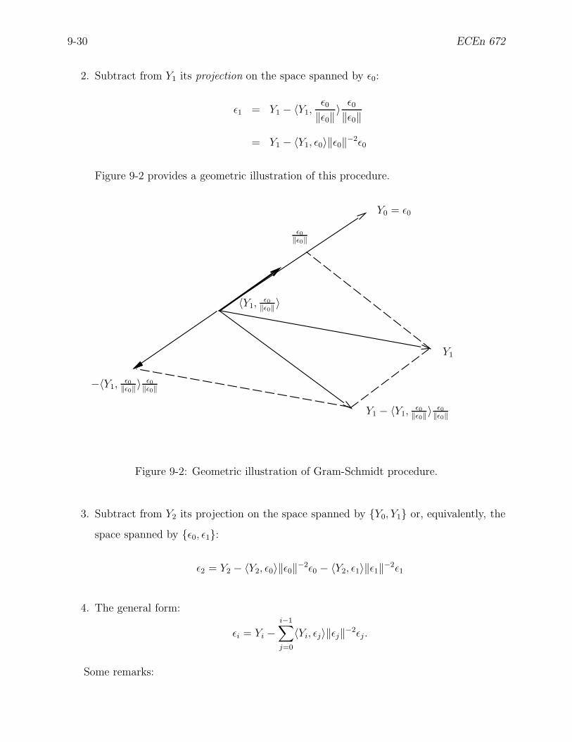
9-30 ECEn 672
2. Subtract from Y1 its projection on the space spanned by ε0:
ε1 = Y1 − 〈Y1,ε0
‖ε0‖〉 ε0
‖ε0‖
= Y1 − 〈Y1, ε0〉‖ε0‖−2ε0
Figure 9-2 provides a geometric illustration of this procedure.
〈Y1,ε0
‖ε0‖〉
ε0‖ε0‖
Y0 = ε0
Y1
−〈Y1,ε0
‖ε0‖〉ε0
‖ε0‖
Y1 − 〈Y1,ε0
‖ε0‖〉ε0
‖ε0‖
Figure 9-2: Geometric illustration of Gram-Schmidt procedure.
3. Subtract from Y2 its projection on the space spanned by Y0, Y1 or, equivalently, the
space spanned by ε0, ε1:
ε2 = Y2 − 〈Y2, ε0〉‖ε0‖−2ε0 − 〈Y2, ε1〉‖ε1‖−2ε1
4. The general form:
εi = Yi −i−1∑
j=0
〈Yi, εj〉‖εj‖−2εj .
Some remarks:

Winter 2009 9-31
• Suppose some εi has zero length? Then Yi is linearly dependent on Y0, · · · , Yi−1 and
RY Y is singular. Hence, the random variable Yi may be omitted. We could employ a
pseudo-inverse and not worry about this potential problem, but for this development
we will assume that such problems have already been eliminated.
• It is sometimes useful to normalize the quantities εi and generate the sequence
νi =εi
‖εi‖, i = 0, 1, · · · ,
then we can write
εi = Yi −i−1∑
j=0
〈Yi, νi〉νi.
• The projection of Yi onto the subspace spanned by Y0, · · · , Yi−1 is the mean square
estimate of Yi given Y0, · · · , Yi−1. We denote this estimate by Yi|i−1. Then
εi = Yi − Yi|i−1.
The random variable εi can be regarded as the “new” information brought by Yi after
Y0, · · · , Yi−1 are known. Recall that εi forms an uncorrelated sequence (a con-
sequence of the Gram-Schmidt construction). The process εi is termed the “new
information” or innovations process (or just the innovations). The process νi is the
normalized innovations process.
• The sequences
ε0, ε1, · · · , εi (Orthogonal)
ν0, ν1, · · · , νi (Orthonormal)
Y0, Y1, · · · , Yi (Arbitrary)
All span the same vector space.
• The Gram-Schmidt procedure is not unique. There are many such orthogonalizing sets
and they can be obtained in many different ways. The important concept is not the
Gram Schmidt procedure, but the properties (i)–(iv) of the innovations that we earlier
noted.

9-32 ECEn 672
Exercise 9-9 Let Yi be a scalar zero-mean stationary random process such that
EYiYj = ρ|i−j|
for some ρ ∈ (0, 1) (Yi is an exponentially correlated process). Verify that
εi = Yi − ρYi−1, ‖εi‖2 = 1 − ρ2
for i = 2, 3.
Exercise 9-10 Suppose the process Yi admits the model:
Yi − ρYi−1 = ui, i = 1, 2, . . . ,
where
Eui = 0
Euiuj =
1 − ρ2 i = j
0 i 6= j, i, j > 0,
EY0 = 0
EY 20 = 1
EY0ui = 0, i > 0.
Verify that this model yields the correlation function of the form EYiYj = ρ|i−j|.
Exercise 9-11 Suppose N independent samples of a random variable, X, are taken, denoted
by x1, x2, · · · , xN . Find the value x that minimizes the quantity
N∑
i=1
(x − xi)2
and interpret the result.
Suppose you take N observations of a certain quantity and wish to compute the mean-
square fit to a constant. Write a conventional expression to do this. Now, suppose you take
one more observation. Show how to express the new average (over N + 1 observations) in
terms of the old average (over N observations) and the (N + 1)st observation. Comment
regarding the computational complexity for your new approach versus. the conventional ap-
proach.

Winter 2009 9-33
Exercise 9-12 Let YN0 denote the linear subspace spanned by the set of observations YiN
i=0 =
Y0, Y1, . . . , YN.Let X be such that
E(X − X)Z = 0
for all Z ∈ YN0 (that is, X is the orthogonal projection of X onto YN
0 ). Also, let X be any
other estimate in YN0 . Prove that
E(X − X)2 ≥ E(X − X)2
and, therefore, that X is the mean square estimate of X given YiNi=0. This proves that
orthogonality is a sufficient condition for minimum mean-square estimation.
To prove that orthogonality is also a necessary condition, suppose that X ∈ YN0 is another
estimate for X and that there is a Z ∈ YN0 such that E(X−X)Z 6= 0. Define a new estimator
X by
X = X +E(X − X)Z
EZ2 Z.
(Does this remind you of anything? Also, why is EZ2 > 0?) Show that
E(X − X)2 < E(X − X)2,
which implies that X is a better estimator than X, so X cannot minimize the mean-square
error.
9.10 Estimation Given the Innovations Process
Since the observed process Yi and the innovations process εi span the same space, it
follows from the projection concept that the estimate of X given Yi must be identical with
the estimate of X given εi. Let us define
X|Ndef= the estimate of X given Y0, . . . , YN.
Then, equivalently,
X|N = the estimate of X given ε0, . . . , εN.
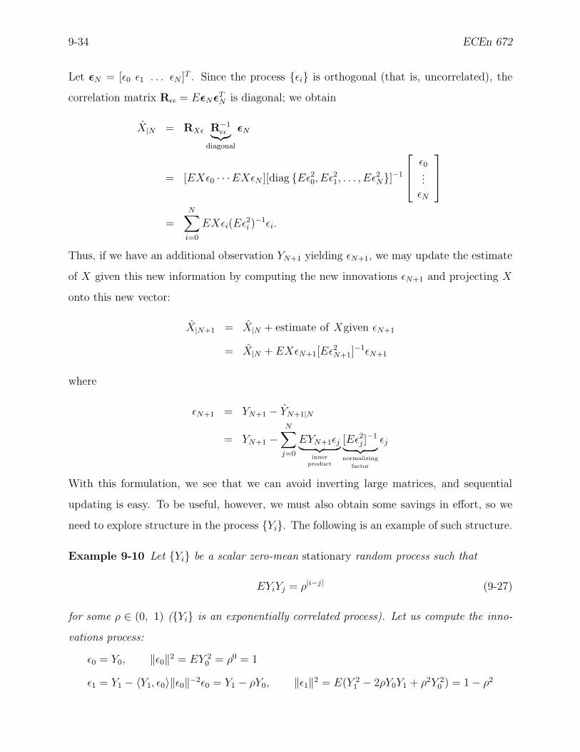
9-34 ECEn 672
Let εN = [ε0 ε1 . . . εN ]T . Since the process εi is orthogonal (that is, uncorrelated), the
correlation matrix Rεε = EεNεTN is diagonal; we obtain
X|N = RXε R−1εε
︸︷︷︸
diagonal
εN
= [EXε0 · · ·EXεN ][diag Eε20, Eε2
1, . . . , Eε2N]−1
ε0...
εN
=
N∑
i=0
EXεi(Eε2i )
−1εi.
Thus, if we have an additional observation YN+1 yielding εN+1, we may update the estimate
of X given this new information by computing the new innovations εN+1 and projecting X
onto this new vector:
X|N+1 = X|N + estimate of Xgiven εN+1
= X|N + EXεN+1[Eε2N+1]
−1εN+1
where
εN+1 = YN+1 − YN+1|N
= YN+1 −N∑
j=0
EYN+1εj︸ ︷︷ ︸
innerproduct
[Eε2j ]
−1
︸ ︷︷ ︸normalizing
factor
εj
With this formulation, we see that we can avoid inverting large matrices, and sequential
updating is easy. To be useful, however, we must also obtain some savings in effort, so we
need to explore structure in the process Yi. The following is an example of such structure.
Example 9-10 Let Yi be a scalar zero-mean stationary random process such that
EYiYj = ρ|i−j| (9-27)
for some ρ ∈ (0, 1) (Yi is an exponentially correlated process). Let us compute the inno-
vations process:
ε0 = Y0, ‖ε0‖2 = EY 20 = ρ0 = 1
ε1 = Y1 − 〈Y1, ε0〉‖ε0‖−2ε0 = Y1 − ρY0, ‖ε1‖2 = E(Y 21 − 2ρY0Y1 + ρ2Y 2
0 ) = 1 − ρ2
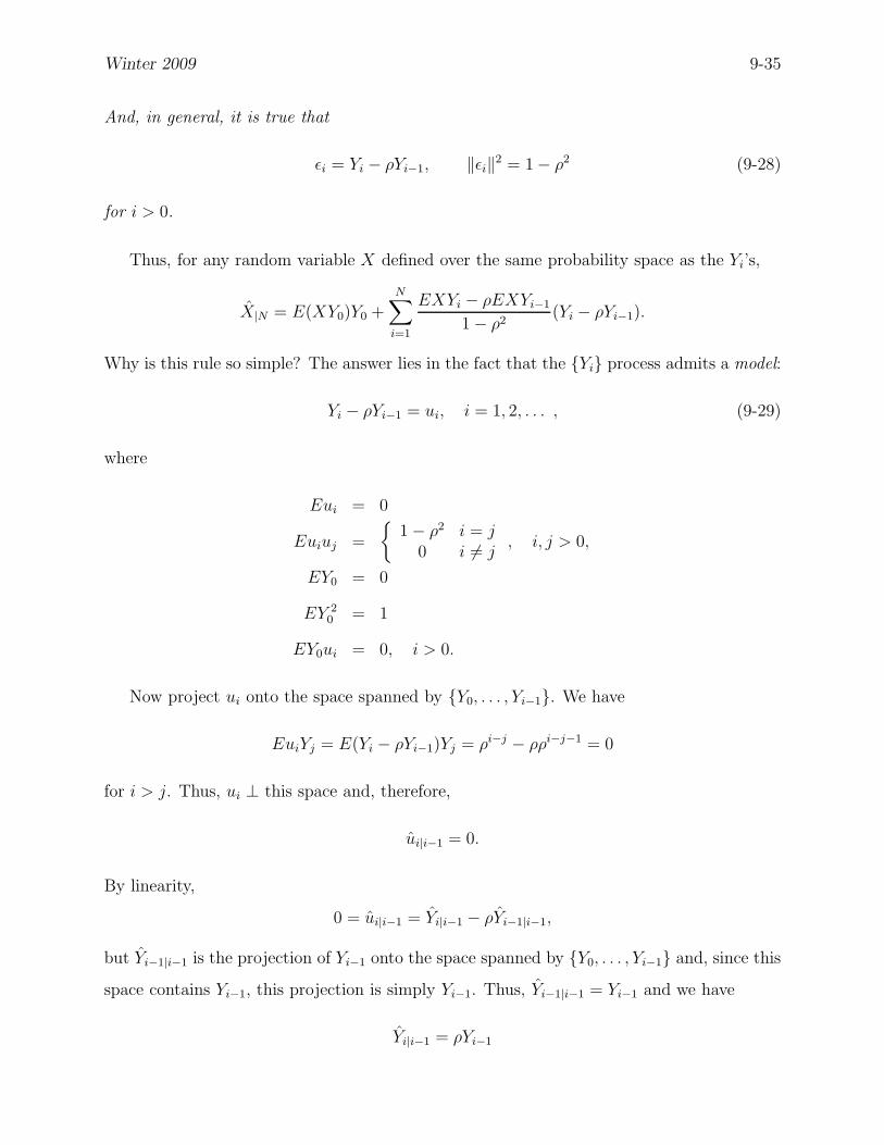
Winter 2009 9-35
And, in general, it is true that
εi = Yi − ρYi−1, ‖εi‖2 = 1 − ρ2 (9-28)
for i > 0.
Thus, for any random variable X defined over the same probability space as the Yi’s,
X|N = E(XY0)Y0 +
N∑
i=1
EXYi − ρEXYi−1
1 − ρ2(Yi − ρYi−1).
Why is this rule so simple? The answer lies in the fact that the Yi process admits a model:
Yi − ρYi−1 = ui, i = 1, 2, . . . , (9-29)
where
Eui = 0
Euiuj =
1 − ρ2 i = j
0 i 6= j, i, j > 0,
EY0 = 0
EY 20 = 1
EY0ui = 0, i > 0.
Now project ui onto the space spanned by Y0, . . . , Yi−1. We have
EuiYj = E(Yi − ρYi−1)Yj = ρi−j − ρρi−j−1 = 0
for i > j. Thus, ui ⊥ this space and, therefore,
ui|i−1 = 0.
By linearity,
0 = ui|i−1 = Yi|i−1 − ρYi−1|i−1,
but Yi−1|i−1 is the projection of Yi−1 onto the space spanned by Y0, . . . , Yi−1 and, since this
space contains Yi−1, this projection is simply Yi−1. Thus, Yi−1|i−1 = Yi−1 and we have
Yi|i−1 = ρYi−1

9-36 ECEn 672
so, therefore,
εi = Yi − Yi|i−1 = Yi − ρYi−1.
Thus, for this problem, the innovations are the white-noise inputs of the model; that is, we
may take εi = ui.
This example is that of a first-order auto-regressive (AR) process. In general, an nth
order AR process is of the form
Yi − ρ1Yi−1 − · · · − ρnYi−n = ui, i > 0,
with
Euiuj = Qδij
EuiYj = 0 j ∈ 0, . . . , i − n.
9.11 Innovations and Matrix Factorizations
Let us continue with the previous example, and compute R−1Y Y as an exercise and see what
develops. First, note that we can arrange the innovations as
ε0
ε1...
εN
=
1 0 · · · · · · 0−ρ 1 0 · · · 0...
. . .. . . 0
......
.... . .
. . ....
0 · · · · · · −ρ 1
︸ ︷︷ ︸
W
Y0
Y1...
YN
or
ε = WY
where W is a lower-triangular matrix. Let
Rεε =
1 0 · · · · · · 00 1 − ρ2 0 · · · 0...
.... . .
......
......
.... . .
...0 · · · · · · 0 1 − ρ2
,
a diagonal matrix. But
Rεε = EεεT = WEYYTWT = WRY Y WT (9-30)
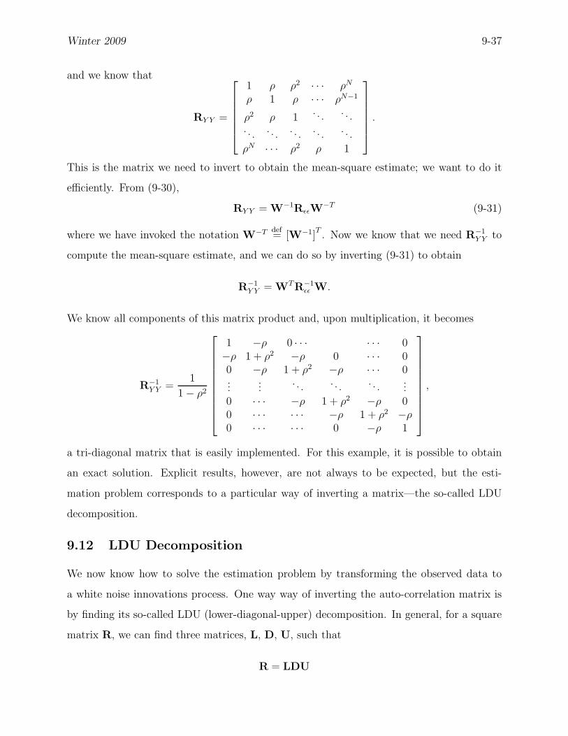
Winter 2009 9-37
and we know that
RY Y =
1 ρ ρ2 · · · ρN
ρ 1 ρ · · · ρN−1
ρ2 ρ 1. . .
. . .. . .
. . .. . .
. . .. . .
ρN · · · ρ2 ρ 1
.
This is the matrix we need to invert to obtain the mean-square estimate; we want to do it
efficiently. From (9-30),
RY Y = W−1RεεW−T (9-31)
where we have invoked the notation W−T def= [W−1]
T. Now we know that we need R−1
Y Y to
compute the mean-square estimate, and we can do so by inverting (9-31) to obtain
R−1Y Y = WTR−1
εε W.
We know all components of this matrix product and, upon multiplication, it becomes
R−1Y Y =
1
1 − ρ2
1 −ρ 0 · · · · · · 0−ρ 1 + ρ2 −ρ 0 · · · 00 −ρ 1 + ρ2 −ρ · · · 0...
.... . .
. . .. . .
...0 · · · −ρ 1 + ρ2 −ρ 00 · · · · · · −ρ 1 + ρ2 −ρ0 · · · · · · 0 −ρ 1
,
a tri-diagonal matrix that is easily implemented. For this example, it is possible to obtain
an exact solution. Explicit results, however, are not always to be expected, but the esti-
mation problem corresponds to a particular way of inverting a matrix—the so-called LDU
decomposition.
9.12 LDU Decomposition
We now know how to solve the estimation problem by transforming the observed data to
a white noise innovations process. One way way of inverting the auto-correlation matrix is
by finding its so-called LDU (lower-diagonal-upper) decomposition. In general, for a square
matrix R, we can find three matrices, L, D, U, such that
R = LDU

9-38 ECEn 672
where L is lower-triangular, D is diagonal, and U is upper-triangular in structure. Further-
more, if the matrix R is symmetric, we may find a decomposition such that U = LT . Thus,
since the auto-correlation matrix RY Y is symmetric, there exist matrices L and D such that
RY Y = LDLT . (9-32)
In the previous example, we may identify
L = W−1
D = Rεε.
9.13 Cholesky Decomposition
Since the matrix we are inverting is positive-definite (that is, has all strictly positive eigenval-
ues), it is possible to refine the LDU decomposition further. Since RY Y > 0 implies Rεε > 0,
we can define a triangular square-root matrix, denoted D12 , such that
D = D12 D
T2 ,
where we have introduced a common notational shorthand: DT2
def=[
D12
]T
. We may then
write (9-32) as
RY Y = LLT,
where Ldef= LD
12 , which is known as the Cholesky decomposition of RY Y . Then
R−1Y Y = L
−TL
−1= W
TW
where we define
W = L−1
= R− 1
2εε W.
The stochastic interpretation of the Cholesky decomposition is as follows: Since ε = WY,
we have Y = W−1ε, thus
RY ε = EYε = W−1Rεε,
so W−1 = RY εR−1εε . Thus, we obtain L = RY εR
−1εε and the LDLT decomposition is
RY Y = RY εR−1εε RεεR
−1εε RT
Y ε = RY εR−1εε RT
Y ε.

Winter 2009 9-39
Also, the matrix W gives the normalized innovations
ν = WY.
Consequently,
L = RY ν = RY εR− 1
2εε ,
and the Cholesky decomposition is also
RY Y = RY νRTY ν .
Reasons for Discussion.
• A standard method for inverting a positive-definite matrix is to make a Cholesky
decomposition RY Y = LLT
and to compute R−1Y Y = L
−TL
−1. This is because it is
easy to invert triangular matrices. Then the general estimation formula becomes
X|N = RXY R−1Y Y Y
= RXY WTWY
= RXY WTR−T
2εε R
− 12
εε WY
= E(XYT )WTR−1εε ε
= E(XεT )R−1εε ε
= RXεR−1εε ε,
the innovations form of the estimator. So the innovations method is equivalent to the
Cholesky factorization method of computing R−1Y Y and X|N .
• Often, additional information is available in the form of a process model, which yields
a fast way of computing the innovations. A fast algorithm is one which will invert RY Y
in fewer than O(N3) operations. If we assume stationarity, we can get the number of
operations down to O(N2), and if we can invoke an AR model, we can get the number
of operations down to O(N log N) (similar in speed to the FFT).

9-40 ECEn 672
9.14 White Noise Interpretations
It may seem counter intuitive that a white noise process could contain information, but we
are claiming that the innovations process, which is a zero-mean uncorrelated process and,
therefore, a white noise process, contains exactly the same information as does the original
data set. Perhaps the best way to convince yourself that this is so is to review how the
innovations are obtained. Recall that we set forth five desirable properties when introducing
the possibility of transforming the data. Of those, the notions of causal and causally invertible
are of central importance. To restate:
• The notion of causality is perhaps best viewed in the context of a process for which
the indexing set is associated with some physical parameter. We have been dealing
with an arbitrary process Yi, where the indexing parameter i is simply a non-negative
integer. For many applications, this indexing set will correspond to time. For example,
the sequence Yi might be derived by sampling a waveform at times ti, i = 0, 1, 2, . . ..
To say that the transformation from Yi to εi is causal is to say that we do not need
future values of Yi to compute past or present values of εi. This makes intuitive sense;
there are many physical processes which admit a causal model, and we get a lot of
mileage out of this notion. But what does causality mean in, say, spatial coordinates,
such as with imagery. It does not make intuitive sense to claim that the right-hand
pixel precedes, in any sense, the left-hand pixel. Causal transforms, in this context,
might be much less desirable than non-causal ones that do not force irrelevant structure
onto the data.
Perhaps the best way to develop an intuition about innovations is to think of them
in the Gram-Schmidt context, where they may be viewed as a way of orthogonalizing
an oblique coordinate system. The abstract vector space idea is very powerful; It will
surface many times in our development of estimation theory.
• The notion of causal invertibility is also of central importance. This concept simply
means that it is possible to reverse the transformation; that is, to recover Yi from
εi.

Winter 2009 9-41
Thus, it is in this sense of causality and causal invertibility that we may claim that the
innovations sequence is informationally equivalent to the original process. It can be
shown, but we will not attempt it here, that, in the context of information theory, the
mutual information between X and Yi is exactly the same as the mutual information
between X and εi. Thus, the innovations transformation is one case where the
information processing lemma leads to strict equality. That lemma, incidentally, will
tell us that it is not possible to increase the information content by any operations on
the data; we may at best preserve it. But the fact that such an information preserving
transform exists and is useful is in important theoretical fact in and of itself!
9.15 More On Modeling
Thus far, we have developed the notion of innovations and have shown that they are nothing
more than a very special coordinate transform of the data. This fact would be of only
academic interest if we could not exploit additional structure in the data to speed up the
calculations. We have given one example to show that, if the process admits an auto-
regressive (AR) model, then significant computational savings can be achieved. This is one
reason why such models are so common on data analysis. For example, they have long been
used in statistics, economics, etc. But AR models work only for stationary, linear processes
(although this can be overcome to some extent—witness the work done in speech processing,
which has long made use of such models. But that gets more to the practitioners art, and
we have yet to develop the theory.
There is another large class of models that attracts our attention: state-space models.
These models, though usually linear, need not be be stationary. It can be easily shown
that all AR models can be re-cast in a state-space formulation, so we really give up nothing
by concentrating on the later class of models. The relaxation of the stationarity constraint
makes it well worth our while to do so, since, as we will see, state-space is a natural and
very rich place to do our analysis. In fact, the constant parameter estimation problem that
we have just solved can also be easily formulated in state-space. So we have a lot to gain
and little to lose in concentrating, for the rest of this development, on state-space models.

10-42 ECEn 672
10 Estimation of State Space Systems
10.1 Innovations for Processes with State Space Models
Suppose the observed process admits a model of the form
Yi = HiXi + Vi, i = 0, 1, 2, · · · , (10-33)
where Xi is an n-dimensional state vector obeying the difference equation
Xi+1 = FiXi + GiUi, i = 0, 1, 2, · · · . (10-34)
Here, the observations consists of a sequence of m-dimensional vectors Yi, as opposed
to the sequence of scalars that we have thus far encountered. Also, rather than just one
parameter vector X to estimate, there is an entire sequence of them, Xi. The Matrices Fi,
Gi, and Hi are termed system matrices and are assumed known. The processes Vi and
Ui are termed observation noise and and process noise, respectively. They are stochastic
components of the system.
Notation Change. In the sequel, we shall be be considering states, inputs, and outputs
as random variables unless otherwise explicitly stated. To simplify notation and come into
conformity with 30 years of engineering usage in estimation theory, we will use lower-case
symbols to denote these random variables.
In statistics, the standard notation for a random variable is to use a capital symbol, and
we have retained that usage up to this point, mainly to reinforce the concept that we are
dealing with random variables and not their actual values (we have had very little to say
about actual values of these random variables). But we will now depart from the traditional
notation of statistics.
Thus, we may rewrite (10-33) and (10-34) as
yi = Hixi + vi, i = 0, 1, 2, · · · , (10-35)
xi+1 = Fixi + Giui, i = 0, 1, 2, · · · , (10-36)
where we assume that yi is an m-dimensional vector, xi is an n-dimensional vector, Hi is
an m× n matrix, vi is an m-dimensional vector, u is a p-dimensional vector, Fi is an n × n
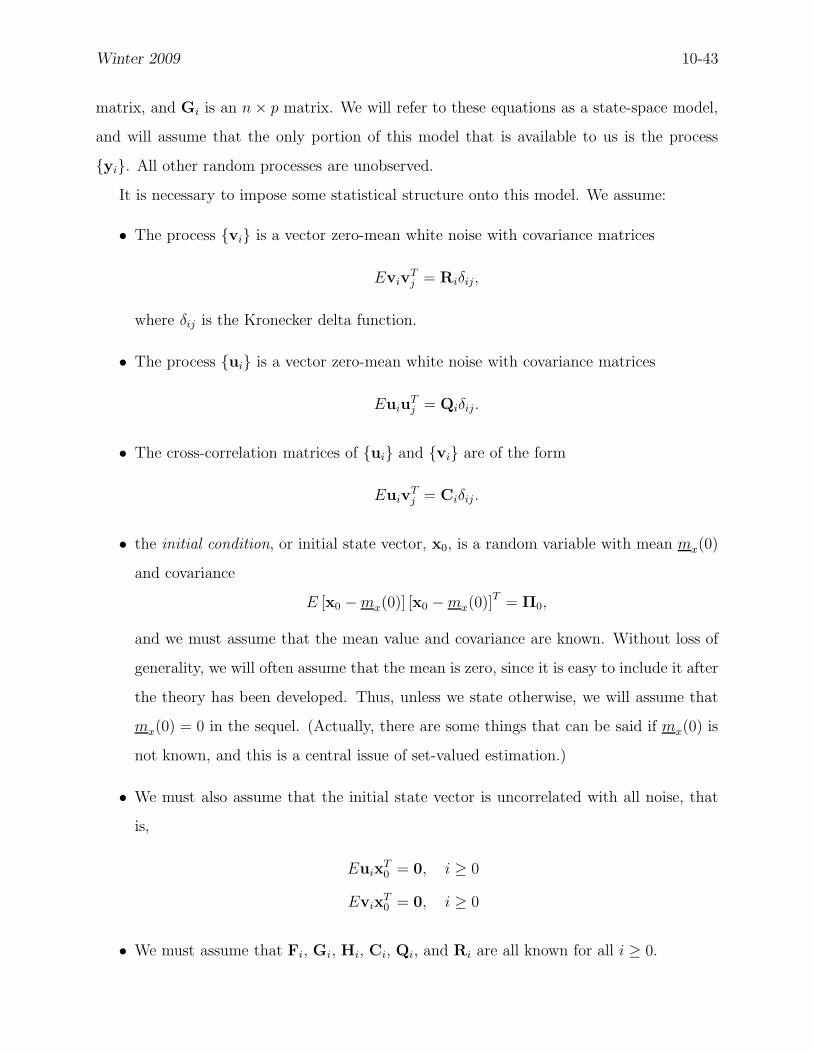
Winter 2009 10-43
matrix, and Gi is an n × p matrix. We will refer to these equations as a state-space model,
and will assume that the only portion of this model that is available to us is the process
yi. All other random processes are unobserved.
It is necessary to impose some statistical structure onto this model. We assume:
• The process vi is a vector zero-mean white noise with covariance matrices
EvivTj = Riδij,
where δij is the Kronecker delta function.
• The process ui is a vector zero-mean white noise with covariance matrices
EuiuTj = Qiδij .
• The cross-correlation matrices of ui and vi are of the form
EuivTj = Ciδij .
• the initial condition, or initial state vector, x0, is a random variable with mean mx(0)
and covariance
E [x0 − mx(0)] [x0 − mx(0)]T = Π0,
and we must assume that the mean value and covariance are known. Without loss of
generality, we will often assume that the mean is zero, since it is easy to include it after
the theory has been developed. Thus, unless we state otherwise, we will assume that
mx(0) = 0 in the sequel. (Actually, there are some things that can be said if mx(0) is
not known, and this is a central issue of set-valued estimation.)
• We must also assume that the initial state vector is uncorrelated with all noise, that
is,
EuixT0 = 0, i ≥ 0
EvixT0 = 0, i ≥ 0
• We must assume that Fi, Gi, Hi, Ci, Qi, and Ri are all known for all i ≥ 0.
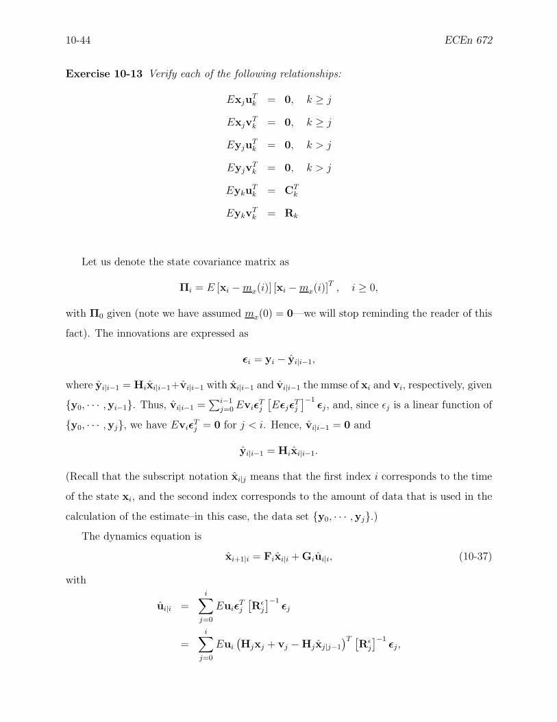
10-44 ECEn 672
Exercise 10-13 Verify each of the following relationships:
ExjuTk = 0, k ≥ j
ExjvTk = 0, k ≥ j
EyjuTk = 0, k > j
EyjvTk = 0, k > j
EykuTk = CT
k
EykvTk = Rk
Let us denote the state covariance matrix as
Πi = E [xi − mx(i)] [xi − mx(i)]T , i ≥ 0,
with Π0 given (note we have assumed mx(0) = 0—we will stop reminding the reader of this
fact). The innovations are expressed as
εi = yi − yi|i−1,
where yi|i−1 = Hixi|i−1+vi|i−1 with xi|i−1 and vi|i−1 the mmse of xi and vi, respectively, given
y0, · · · ,yi−1. Thus, vi|i−1 =∑i−1
j=0 EviεTj
[Eεjε
Tj
]−1εj , and, since εj is a linear function of
y0, · · · ,yj, we have EviεTj = 0 for j < i. Hence, vi|i−1 = 0 and
yi|i−1 = Hixi|i−1.
(Recall that the subscript notation xi|j means that the first index i corresponds to the time
of the state xi, and the second index corresponds to the amount of data that is used in the
calculation of the estimate–in this case, the data set y0, · · · ,yj.)The dynamics equation is
xi+1|i = Fixi|i + Giui|i, (10-37)
with
ui|i =
i∑
j=0
EuiεTj
[Rε
j
]−1εj
=
i∑
j=0
Eui
(Hjxj + vj − Hjxj|j−1
)T [Rε
j
]−1εj ,

Winter 2009 10-45
where
Rεj
def= Eεjε
Tj .
But EuixTj = 0 for j ≤ i and Euiv
Tj = Ciδij by the modeling hypothesis, and Euix
Tj|j−1 = 0
for j ≤ i since xj|j−1 depends only upon y0, · · · ,yj−1 which is orthogonal to vi, also by
the modeling hypothesis. Thus,
ui|i =
i∑
j=0
EuivTj
[Rε
j
]−1εj = Ci [R
εi]−1
εi.
Consequently, (10-37) becomes
xi+1|i = Fixi|i + GiCi [Rεi]−1
εi. (10-38)
As a point of terminology, we often refer to xi|i as the filtered estimate of xi, and to xi|i−1
as the (one-step) predicted estimate of xi. Also, we adopt the convention that observations
begin at i = 0 (usually, the index i will correspond to time).
We may view the predicted estimate (10-38) as a “time-update” equation, since it shows
how the state evolves in time from i to i + 1 in the absence of data. We can also think of
obtaining a “measurement-update” equation to tell us how to convert the predicted estimate,
xi+1|i into a filtered estimate, xi+1|i+1. Recall the basic formula for the estimation of any
random variable X given the innovations:
X|N = X|N−1 + EXεTN [Rε
N ]−1εN .
Now set
N = i + 1
X = xi+1
to obtain
xi+1|i+1 = xi+1|i + E[xi+1ε
Ti+1
] [Rε
i+1
]−1εi+1. (10-39)
Equations (10-38) and (10-39) constitute a set of recursive equations, and indicate the
way the state estimates evolve as observations are made as time progresses. It remains to
compute E[xiε
Ti
]and Rε
i. We will shortly obtain expressions for these quantities, but before
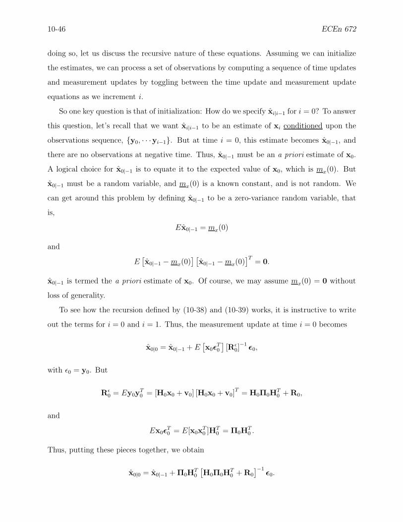
10-46 ECEn 672
doing so, let us discuss the recursive nature of these equations. Assuming we can initialize
the estimates, we can process a set of observations by computing a sequence of time updates
and measurement updates by toggling between the time update and measurement update
equations as we increment i.
So one key question is that of initialization: How do we specify xi|i−1 for i = 0? To answer
this question, let’s recall that we want xi|i−1 to be an estimate of xi conditioned upon the
observations sequence, y0, · · ·yi−1. But at time i = 0, this estimate becomes x0|−1, and
there are no observations at negative time. Thus, x0|−1 must be an a priori estimate of x0.
A logical choice for x0|−1 is to equate it to the expected value of x0, which is mx(0). But
x0|−1 must be a random variable, and mx(0) is a known constant, and is not random. We
can get around this problem by defining x0|−1 to be a zero-variance random variable, that
is,
Ex0|−1 = mx(0)
and
E[x0|−1 − mx(0)
] [x0|−1 − mx(0)
]T= 0.
x0|−1 is termed the a priori estimate of x0. Of course, we may assume mx(0) = 0 without
loss of generality.
To see how the recursion defined by (10-38) and (10-39) works, it is instructive to write
out the terms for i = 0 and i = 1. Thus, the measurement update at time i = 0 becomes
x0|0 = x0|−1 + E[x0ε
T0
][Rε
0]−1
ε0,
with ε0 = y0. But
Rε0 = Ey0y
T0 = [H0x0 + v0] [H0x0 + v0]
T = H0Π0HT0 + R0,
and
Ex0εT0 = E[x0x
T0 ]HT
0 = Π0HT0 .
Thus, putting these pieces together, we obtain
x0|0 = x0|−1 + Π0HT0
[H0Π0H
T0 + R0
]−1ε0.

Winter 2009 10-47
We can then predict to i = 1, yielding
x1|0 = F0x0|0 + G0C0[Rε0]−1ε0
= F0x0|0 + G0C0[H0Π0HT0 + R0]
−1ε0.
One can continue in this way to obtain the general case, but a little experimentation will
convince you that things get a bit messy, although it should be clear enough, in principle,
how to proceed.
Before developing the general solution to this recursive system, we will continue our
digression and generate some variations on the time- and measurement-update equations.
Substitute (10-38) into (10-39) to obtain
xi+1|i+1 = Fixi|i + E[xi+1ε
Ti+1
] [Rε
i+1
]−1εi+1 + GiCi [R
εi]−1
εi (10-40)
where
εi+1 = yi+1 −Hi+1xi+1|i
= yi+1 −Hi+1Fixi|i − Hi+1GiCi [Rεi]−1
εi
with ε0 = y0. Note that (10-40) employs only filtered estimates.
Alternatively, multiply both sides of (10-39) by Fi+1 and substitute into (10-38) to get
(with i + 1 → i)
xi+1|i = Fixi|i−1 + Ki [Rεi]−1
εi (10-41)
where
εi = yi − Hixi|i−1
with x0|−1 = 0 and
Ki = Exi+1εTi = FiExiε
Ti + GiCi.
Several other variations on these equations are possible. Equation (10-41) involves only
predicted estimates, and is termed the one-step predictor. This formulation is very useful
for theoretical development.
The parameters ExiεTi and Eεiε
Ti do not depend upon the actual observations yi but,
rather, upon the model parameters F, G, H, Q, R, C, and Π0. Thus, they may, if desired, be

10-48 ECEn 672
calculated in advance of the actual data collection. Explicit, closed-form solutions for ExiεTi
and Rεi are not available except in a few very special cases. Recursive ways of computing
them, however, are known—we shall shortly develop the most famous way of doing so.
10.2 Innovations Representations
We recall that the model for the observed process yi, i = 0, 1, · · · is
xi+1 = Fixi + Giui (10-42)
yi = Hixi + vi. (10-43)
We will assume Ex0 = 0 and Ex0xT0 = Π0. This representation of the observations yi, i =
0, 1, · · · will be called, for lack of a better term, the “true” model, since we presumably
base it upon physical principles, and xi is intended to represent the actual, or true state of
the system. But don’t forget that the state is a random process—what does it mean to be
the “true” random state? (Probably not much unless the density function is degenerate.)
We may express the covariance of xi as ExixTi = Πi, and observe that
Exi+1xTi+1
︸ ︷︷ ︸
Πi+1
= E [Fixi + Giui] [Fixi + Giui]T
= Fi ExixTi
︸ ︷︷ ︸
Πi
FTi + FiExiu
Ti GT
i + GiEuixTi FT
i + Gi EuiuTi
︸ ︷︷ ︸
Qi
GTi .
Since, by the modeling assumptions, we have ExiuTi = 0,
Πi+1 = FiΠiFTi + GiQiG
Ti , Π0 given (10-44)
Now let’s think about (10-43) for a moment. In actuality, yi is the only directly observable
one; it is the one we measure. The processes xi, ui, and vi are never directly available.
Equations (10-42) and (10-43) constitute one way to characterize the observations process
yi, but we might rightly ask the question: Are there other ways to model the observations?
The answer is: yes, and it is the so-called innovations model. We have already seen it:
xi+1|i = Fixi|i−1 + Ki [Rεi]−1
εi (10-45)
yi = Hixi|i−1 + εi. (10-46)

Winter 2009 10-49
As far as an observer is concerned, this signal model is just as valid as the “true” signal
model given by (10-42) and (10-43). But there is at least one very big advantage of the
innovations model over the “true” one: we have access to both xi|i−1 and to εi. So let’s
explore the innovations representation a bit further.
We may calculate the covariance of xi as
Exi+1|ixTi+1|i = E
[Fixi|i−1 + Ki [R
εi ]−1
εi
] [Fixi|i−1 + Ki [R
εi]−1
εi
]T
= FiExi|i−1xTi|i−1F
Ti + Fi Exi|i−1ε
Ti
︸ ︷︷ ︸
0
[Rεi]−1 KT
i
+Ki [Rεi]−1 Eεix
Ti|i−1
︸ ︷︷ ︸
0
FTi + Ki [R
εi]−1 Eεiε
Ti
︸ ︷︷ ︸
Rεi
[Rεi ]−1 KT
i . (10-47)
But the innovations εi is orthogonal to the subspace spanned by y0, · · · ,yi−1, and since
xi|i−1 lies in this subspace, we have
Exi|i−1εTi = 0.
If we define
Σi+1|i = Exi+1|ixTi+1|i,
as the covariance of xi+1|i, then (10-47) becomes
Σi+1|i = FiΣi|i−1FTi + Ki [R
εi]−1 KT
i (10-48)
with
Σ0|−1 = Ex0|−1xT0|−1 = 0.
Since we have the state xi associated with the “true” representation of the signal and
the state xi|i−1 associated with the innovations representation of the signal, we may wish to
compare them. Define the predicted state estimation error as
xi|i−1 = xi − xi|i−1,
and let
Pi|i−1def= Exi|i−1x
Ti|i−1
denote the estimation error covariance matrix.

10-50 ECEn 672
We can write the innovations as
εi = yi − Hixi|i−1 = Hixi + vi︸ ︷︷ ︸
yi
−Hixi|i−1
= Hixi|i−1 + vi. (10-49)
Then we can express
Rεi = Eεiε
Ti = Hi Exi|i−1x
Ti|i−1
︸ ︷︷ ︸
Pi|i−1
HTi + HiExi|i−1v
Ti + Evix
Ti|i−1H
Ti + Eviv
Ti
︸ ︷︷ ︸
Ri
.
But
Exi|i−1vTi = 0
since vi is orthogonal to both xi and xi|i−1. Consequently,
Rεi = HiPi|i−1H
Ti + Ri. (10-50)
Also,
ExiεTi = Exi(x
Ti|i−1H
Ti + vT
i )
= ExixTi|i−1H
Ti + Exiv
Ti
︸ ︷︷ ︸
0
= E[xi|i−1 + xi|i−1]xTi|i−1H
Ti
= Exi|i−1xTi|i−1
︸ ︷︷ ︸
0
HTi + Exi|i−1x
Ti|i−1
︸ ︷︷ ︸
Pi|i−1
HTi .
Thus,
ExiεTi = Pi|i−1H
Ti . (10-51)
10.3 A Recursion for Pi|i−1
Since xi|i−1 and xi|i−1 are orthogonal, we have an orthogonal decomposition of xi:
xi = xi|i−1 + xi|i−1.

Winter 2009 10-51
(Recall that orthogonality means uncorrelated.) Consequently, taking the variance of both
sides of this expression (assuming all random variables are zero-mean), we obtain
Πi = ExixTi
= E[xi|i−1 + xi|i−1
] [xi|i−1 + xi|i−1
]T
= Exi|i−1xTi|i−1
︸ ︷︷ ︸
Σi|i−1
+ Exi|i−1xTi|i−1
︸ ︷︷ ︸
0
+ Exi|i−1xTi|i−1
︸ ︷︷ ︸
0
+ Exi|i−1xTi|i−1
︸ ︷︷ ︸
Pi|i−1
,
or
Πi = Σi|i−1 + Pi|i−1. (10-52)
Since Σ0|−1 = 0, we have P0|−1 = Π0.
Rearranging (10-52) and applying (10-44) and (10-48), we have
Pi+1|i = Πi+1 −Σi+1|i
= FiΠiFTi + GiQiG
Ti − FiΣi|i−1F
Ti − Ki [R
εi]−1 KT
i
or
Pi+1|i = FiPi|i−1FTi + GiQiG
Ti −Ki [R
εi]−1 KT
i .
Since
Ki = FiPi|i−1HTi + GiCi
and
Rεi = HiPi|i−1H
Ti + Ri,
we obtain
Pi+1|i = FiPi|i−1FTi + GiQiG
Ti
−[FiPi|i−1H
Ti + GiCi
] [HiPi|i−1H
Ti + Ri
]−1 [FiPi|i−1H
Ti + GiCi
]T(10-53)
with
P0|−1 = Π0. (10-54)
Equation (10-53) is known as a Matrix Riccati difference equation, after the Italian mathe-
matician that first analyzed nonlinear differential equations of the form.
This difference equation is nonlinear, but can be easily solved by recursive means.

10-52 ECEn 672
10.4 The Discrete-Time Kalman Filter
With the development of the matrix Riccati equation (10-53), we have completed every
step needed for the celebrated Kalman filter. We will present two useful ways to express
the Kalman filter; in fact, we have already introduced them. One is the one-step predictor
equation, and the other is the time-update/measurement-update formulation. Let’s see them
both now that we know how to evaluate all of the expectations.
The One-Step Predictor Form
Substitution of (10-50) and (10-51) into (10-41) yields the one-step predictor form of the
Kalman filter:
xi+1|i = Fixi|i−1 +[FiPi|i−1H
Ti + GiCi
] [HiPi|i−1H
Ti + Ri
]−1[yi −Hixi|i−1]
with x0|−1 = mx(0) and Pi|i−1 is given by (10-53) and (10-54).
Time-Update/Measurement-Update Form
Since both the state estimate and the associated error covariance need to be updated, we
will derive time- and measurement-update equations for both of these quantities. First, we
consider the time-update equation for the state. Substitution of (10-50) into (10-38) yields
the time-update equation:
xi+1|i = Fixi|i + GiCi
[HiPi|i−1H
Ti + Ri
]−1[yi − Hixi|i−1]︸ ︷︷ ︸
εi
.
Also, substitution of (10-50) and (10-51) into (10-39) yields the measurement-update equa-
tion:
xi+1|i+1 = xi+1|i + Pi+1|iHTi+1
[Hi+1Pi+1|iH
Ti+1 + Ri+1
]−1[yi+1 − Hi+1xi+1|i]︸ ︷︷ ︸
εi+1
.
The covariance matrix, Pi|i−1, is obtained via (10-53) and (10-54).
Alternate Time-Update/Measurement-Update Form with Ci ≡ 0
The time-update/measurement-update formulation given above is not quite as convenient
as it might be, since both expressions involve the predicted covariance, Pi|i−1. A more
useful representation of the estimator may be obtained when Ci ≡ 0 by developing separate
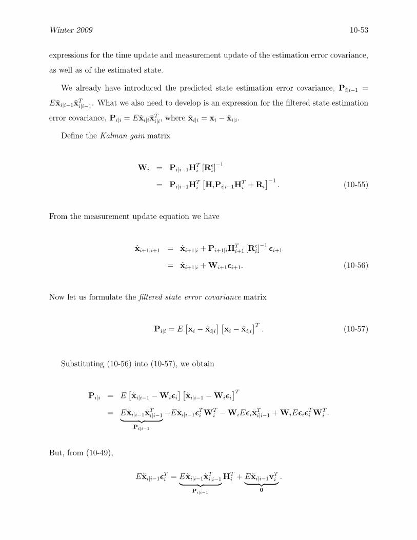
Winter 2009 10-53
expressions for the time update and measurement update of the estimation error covariance,
as well as of the estimated state.
We already have introduced the predicted state estimation error covariance, Pi|i−1 =
Exi|i−1xTi|i−1. What we also need to develop is an expression for the filtered state estimation
error covariance, Pi|i = Exi|ixTi|i, where xi|i = xi − xi|i.
Define the Kalman gain matrix
Wi = Pi|i−1HTi [Rε
i]−1
= Pi|i−1HTi
[HiPi|i−1H
Ti + Ri
]−1. (10-55)
From the measurement update equation we have
xi+1|i+1 = xi+1|i + Pi+1|iHTi+1 [Rε
i]−1
εi+1
= xi+1|i + Wi+1εi+1. (10-56)
Now let us formulate the filtered state error covariance matrix
Pi|i = E[xi − xi|i
] [xi − xi|i
]T. (10-57)
Substituting (10-56) into (10-57), we obtain
Pi|i = E[xi|i−1 −Wiεi
] [xi|i−1 −Wiεi
]T
= Exi|i−1xTi|i−1
︸ ︷︷ ︸
Pi|i−1
−Exi|i−1εTi WT
i −WiEεixTi|i−1 + WiEεiε
Ti WT
i .
But, from (10-49),
Exi|i−1εTi = Exi|i−1x
Ti|i−1
︸ ︷︷ ︸
Pi|i−1
HTi + Exi|i−1v
Ti
︸ ︷︷ ︸
0
.
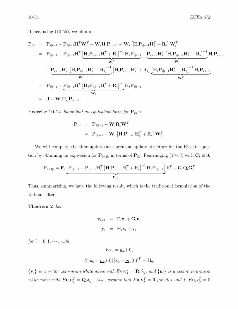
10-54 ECEn 672
Hence, using (10-55), we obtain
Pi|i = Pi|i−1 − Pi|i−1HTi WT
i − WiHiPi|i−1 + Wi
[HiPi|i−1H
Ti + Ri
]WT
i
= Pi|i−1 − Pi|i−1HTi
[HiPi|i−1H
Ti + Ri
]−1HiPi|i−1
︸ ︷︷ ︸
WTi
−Pi|i−1HTi
[HiPi|i−1H
Ti + Ri
]−1
︸ ︷︷ ︸
Wi
HiPi|i−1
+Pi|i−1HTi
[HiPi|i−1H
Ti + Ri
]−1
︸ ︷︷ ︸
Wi
[HiPi|i−1H
Ti + Ri
] [HiPi|i−1H
Ti + Ri
]−1HiPi|i−1
︸ ︷︷ ︸
WTi
= Pi|i−1 − Pi|i−1HTi
[HiPi|i−1H
Ti + Ri
]−1
︸ ︷︷ ︸
Wi
HiPi|i−1
= [I − WiHi]Pi|i−1.
Exercise 10-14 Show that an equivalent form for Pi|i is
Pi|i = Pi|i−1 − WiRεiW
Ti
= Pi|i−1 − Wi
[HiPi|i−1H
Ti + Ri
]WT
i .
We will complete the time-update/measurement-update structure for the Riccati equa-
tion by obtaining an expression for Pi+1|i in terms of Pi|i. Rearranging (10-53) with Ci ≡ 0,
Pi+1|i = Fi
[
Pi|i−1 − Pi|i−1HTi
[HiPi|i−1H
Ti + Ri
]−1HiPi|i−1
]
︸ ︷︷ ︸
Pi|i
FTi + GiQiG
Ti
Thus, summarizing, we have the following result, which is the traditional formulation of the
Kalman filter:
Theorem 2 Let
xi+1 = Fixi + Giui
yi = Hixi + vi
for i = 0, 1, · · · , with
Ex0 = mx(0),
E [x0 − mx(0)] [x0 − mx(0)]T = Π0,
vi is a vector zero-mean white noise with EvivTj = Riδij, and ui is a vector zero-mean
white noise with EuiuTj = Qiδij. Also, assume that Euiv
Tj = 0 for all i and j, Euix
T0 = 0

Winter 2009 10-55
for i ≥ 0, and EvixT0 = 0 for i ≥ 0. Then the linear mean squares estimate of xi given
observations yi, i ≥ 0, is
xi+1|i+1 = xi+1|i + Wi+1
[yi+1 −Hi+1xi+1|i
]
Pi+1|i+1 = Pi+1|i − Wi+1Rεi+1W
Ti+1
= [I −Wi+1Hi+1]Pi+1|i
(measurement update),
andxi+1|i = Fixi|i
Pi+1|i = FiPi|iFTi + GiQiG
Ti
(time update), (10-58)
wherex0|−1 = mx(0)
P0|−1 = Π0
(initial conditions), (10-59)
and
Wi = Pi|i−1HTi
[HiPi|i−1H
Ti + Ri
]−1.
Exercise 10-15 Show that an alternative form of the Riccati equation (assume Ci ≡ 0) is
Pi+1|i = FiPi|i−1
[I + HT
i R−1i HiPi|i−1
]−1FT
i + GiQiGTi .
To establish this result, you may wish to use the following identity:
[I + HTR−1HTP
]−1= I −HT
[R + HPHT
]−1HP,
which in turn is a special case of the famous identity
[A + BCD]−1 = A−1 −A−1B[DA−1B + C−1
]−1DA−1.
This identity is proven in many places—see, for example, the appendix of Kailath’s Linear
Systems. It has great utility in linear estimation theory, and we will see it from time to time.
Exercise 10-16 We are given observations
yi = xi + ni, i = 0,±1,±2, · · ·
where xi and ni are stationary processes with power spectral densities Sx(z) and Sn(z),
respectively (Here, z is the z-transform variable). We shall use a noncausal linear filter with
impulse response hi to estimate xi, that is,
xi =
∞∑
j=−∞hi−jyj

10-56 ECEn 672
Show that the mean-square error, E[xi − xi]2, will be minimized by choosing
H(z) =Sx(z)
Sx(z) + Sn(z).
Exercise 10-17 Define a random process y0, y1, . . . by the following recursive procedure:
Let y0 be a random variable uniformly distributed over (0, 1) and define yk as the fractional
part of 2yk−1, k = 1, 2, . . .. Show that Eyk = 0.5, cov (yk, yi) = 2−|k−i|
12.
Show that Let yk|k−1 = 14
+ 12yk−1, where yk|k−1 is the linear least squares predictor of yk
given y0, . . . , yk−1.Demonstrate that E(yk − yk|k−1)
2 = 116
.
Can you find a better nonlinear predictor? If so, what is it?
NOTE: If y0 = 0.a1a2a3 · · · , observe that the ak will be independent random variables
taking values 0, 1, each with probability 12, and that we shall have
yk = 0.akak+1 · · · =
∞∑
i=1
ak+i
2i.
Exercise 10-18 Consider a process yk with a state-space model
xk+1 = Fxk + Guk, k ≥ 0
yk = Hxk + vk
where
E
ui
vi
x0
[uTj vT
j xT0 ] =
Q C 0CT R 00 0 Π0
δij ,
where δij is the Kronecker delta function. Define Πk = ExkxTk . Show that we can write
EyiyTj =
HFi−jNj + Rδij, i ≥ j
NTi Fj−iHT , i < j
where
Nj = ΠjHT + GC
Exercise 10-19 A process yk is called wide-sense Markov if the linear least squares es-
timate of yk+j, j > 0, given yi, i ≤ k, depends only upon the value of yk. Show that a
process is wide-sense Markov if and only if
f(i, k) = f(i, j)f(j, k), i ≤ j ≤ k,
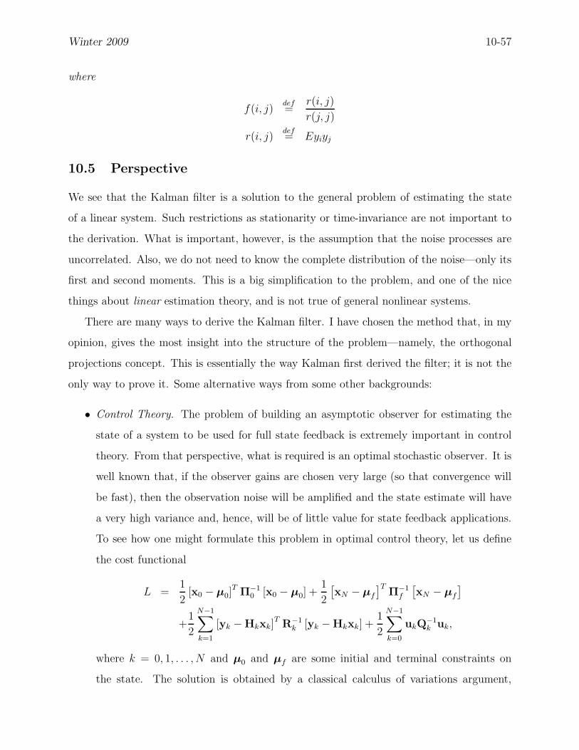
Winter 2009 10-57
where
f(i, j)def=
r(i, j)
r(j, j)
r(i, j)def= Eyiyj
10.5 Perspective
We see that the Kalman filter is a solution to the general problem of estimating the state
of a linear system. Such restrictions as stationarity or time-invariance are not important to
the derivation. What is important, however, is the assumption that the noise processes are
uncorrelated. Also, we do not need to know the complete distribution of the noise—only its
first and second moments. This is a big simplification to the problem, and one of the nice
things about linear estimation theory, and is not true of general nonlinear systems.
There are many ways to derive the Kalman filter. I have chosen the method that, in my
opinion, gives the most insight into the structure of the problem—namely, the orthogonal
projections concept. This is essentially the way Kalman first derived the filter; it is not the
only way to prove it. Some alternative ways from some other backgrounds:
• Control Theory. The problem of building an asymptotic observer for estimating the
state of a system to be used for full state feedback is extremely important in control
theory. From that perspective, what is required is an optimal stochastic observer. It is
well known that, if the observer gains are chosen very large (so that convergence will
be fast), then the observation noise will be amplified and the state estimate will have
a very high variance and, hence, will be of little value for state feedback applications.
To see how one might formulate this problem in optimal control theory, let us define
the cost functional
L =1
2[x0 − µ0]
T Π−10 [x0 − µ0] +
1
2
[xN − µf
]TΠ−1
f
[xN − µf
]
+1
2
N−1∑
k=1
[yk −Hkxk]T R−1
k [yk −Hkxk] +1
2
N−1∑
k=0
ukQ−1k uk,
where k = 0, 1, . . . , N and µ0 and µf are some initial and terminal constraints on
the state. The solution is obtained by a classical calculus of variations argument,

10-58 ECEn 672
which yields the minimization of J subject to the system state model constraints.
We will not pursue this discussion here in any detail. The solution is in the form
of a so-called two-point boundary-value problem (TPBVP). The resulting solution is,
however, not exactly the Kalman filter. Recall that the Kalman filter is causal, in that
the innovations are causally and inversely causally related to the observations sequence.
Here, however, we are using all of the data simultaneously to determine the optimal
state estimates (optimal in the sense that they minimize the cost functional J). The
solution turns out be what is called the optimal smoother and, by careful identification
of terms, one can see that the Kalman filter is embedded in it. We will not develop
these equations in this class; I mention them only to provide a cultural background for
this very important body of theory that we are developing.
• Probability theory. The orthogonal projections approach we have taken for the devel-
opment of the Kalman filter does not rely on anything more than knowledge of the
first and second moments of the distributions of all the random processes involved. If
we do indeed have complete knowledge of all distributions involved, we should perhaps
wonder if we might do better than just having partial knowledge. This is a realistic
question to address, and the answer is, for linear Gaussian systems, we do not buy any-
thing more!!. The reason is, succinctly, that the first and second moments completely
specify the Gaussian distribution.
• Statistical methods. One might consider the estimation problem from a couple of other
aspects. For example, techniques such as minimum variance and maximum likelihood
have great utility in classical statistics—perhaps they will lead to a different (and,
maybe, better) estimator. Fond hope. It is not too hard to see that the Kalman
filter admits interpretations as both a minimum variance estimator and a maximum
likelihood estimator.
The fact is, that, under fairly wide and applicable conditions, the least-squares, condi-
tional expectations, maximum likelihood, minimum variance, and optimal control interpre-
tations of the Kalman filter are all equivalent. This is quite remarkable to me, and I do not
pretend to fathom the deepest meanings of this happy circumstance. I believe the answer

Winter 2009 10-59
lies in the basic structure of linear systems, and I think that the orthogonality principle is
the most basic mathematic foundation, but who knows . . .
10.6 Kalman Filter Example
The purpose of this example is to gain some intuition and experience in the operation of
the Kalman filter. Consider a six-state linear system with a three-dimensional observations
vector corresponding to three-dimensional equations of motion of a moving vehicle. The
observations consist of noisy samples of the vehicle position.
10.6.1 Model Equations
Let x = [x, y, z, x, y, z]T denote the kinematic state of a target in some convenient coordinate
system. The dynamics equation is
xi =
1 0 0 ∆ 0 00 1 0 0 ∆ 00 0 1 0 0 ∆0 0 0 1 0 00 0 0 0 1 00 0 0 0 0 1
︸ ︷︷ ︸
F
xi−1 +
uxi
uyi
uzi
uxi
uyi
uzi
︸ ︷︷ ︸
ui
,
where ∆ is the sample interval. (We assume that G ≡ I.)
For a physical observation system, we will not usually be able to measure position di-
rectly. Let us assume, however, that an optical angle-of-arrival sensor system is available (for
example, from infra-red sensors), yielding azimuth and elevation angles of the vehicle. Fur-
ther, we assume that the sensor is sufficiently far from the target that a linearized model is
adequate. For convenience we also assume that the measurement units are scaled such that,
say, one unit of angle corresponds to one meter of displacement, and that the coordinate
system is resolved along the azimuth and elevation angles. Then the observations vector is
yi =
[yi1
yi2
]
=
1 0 0 0 0 00 1 0 0 0 00 0 1 0 0 0
︸ ︷︷ ︸
H
xi + vi.
Now let’s set up the Q, Π0, and R matrices. The only slightly tricky thing is the
Q matrix, so let’s tackle it first. You might have been wondering why we set G = I

10-60 ECEn 672
and set up four different process noise components in ui. The reason has to do with the
continuous-discrete conversion of the dynamics equations. The discrete-time model given
above is derived from the continuous-time dynamics equation:
xt
yt
zt
xt
yt
zt
︸ ︷︷ ︸
xt
=
0 0 0 1 0 00 0 0 0 1 00 0 0 0 0 10 0 0 0 0 00 0 0 0 0 00 0 0 0 0 0
︸ ︷︷ ︸
F
xt
yt
zt
xt
yt
zt
︸ ︷︷ ︸
xt
+
0 0 00 0 00 0 01 0 00 1 00 0 1
︸ ︷︷ ︸
G
wxt
wyt
wzt
︸ ︷︷ ︸
wt
(10-60)
where the system matrices F and G are defined in (10-60) and wt is a continuous-time white
noise.
To simplify the following development, let’s assume a constant sampling rate, ∆. To
convert this equation to discrete-time, we first must calculate the state transition matrix, F.
This is easily done by setting
Φ(t) = exp Ft = exp
0 0 0 1 0 00 0 0 0 1 00 0 0 0 0 10 0 0 0 0 00 0 0 0 0 00 0 0 0 0 0
t
=
1 0 0 t 0 00 1 0 0 t 00 0 1 0 0 t0 0 0 1 0 00 0 0 0 1 00 0 0 0 0 1
.
For a step-size of ti+1 − ti, the transition matrix becomes, therefore,
F = Φ(ti+1 − ti).
Now to calculate Q. Let us express the covariance of the continuous-time process noise
wt as
Ewtws = Qδ(t − s) =
q2x 0 00 q2
y 00 0 q2
z
δ(t − s).
The discrete-time process noise is obtained via the superposition integral as
ui =
∫ ti+1
ti
Φ(t)Gwtdt.
Clearly, EuiuTj = 0 for i 6= j, and
EuiuTi =
∫ ti+1
ti
∫ ti+1
ti
Φ(ti+1 − t)G Ewtw
Ts
︸ ︷︷ ︸
Qδ(t−s)
GT ΦT (ti+1 − s)dtds
=
∫ ti+1
ti
Φ(ti+1 − t)GQGT ΦT (ti+1 − t)dt.
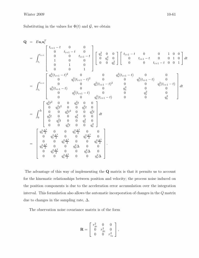
Winter 2009 10-61
Substituting in the values for Φ(t) and G, we obtain
Q = EuiuTi
=
∫ ti+1
ti
ti+1 − t 0 00 ti+1 − t 00 0 ti+1 − t
1 0 00 1 00 0 1
q2x 0 00 q2
y 0
0 0 q2z
ti+1 − t 0 0 1 0 00 ti+1 − t 0 0 1 00 0 ti+1 − t 0 0 1
dt
=
∫ ti+1
ti
q2x(ti+1 − t)2 0 0 q2
x(ti+1 − t) 0 00 q2
y(ti+1 − t)2 0 0 q2y(ti+1 − t) 0
0 0 q2z (ti+1 − t)2 0 0 q2
y(ti+1 − t)
q2x(ti+1 − t) 0 0 q2
x 0 00 q2
y(ti+1 − t) 0 0 q2y 0
0 0 q2z (ti+1 − t) 0 0 q2
z
dt
=
∫ ∆
0
q2xt
2 0 0 q2xt 0 0
0 q2yt
2 0 0 q2yt 0
0 0 q2z t
2 0 0 q2z t
q2xt 0 0 q2
x 0 00 q2
yt 0 0 q2y 0
0 0 q2z t 0 0 q2
z
dt
=
q2x
∆3
3 0 0 q2x
∆2
2 0 0
0 q2y
∆3
3 0 0 q2y
∆2
2 0
0 0 q2z
∆3
3 0 0 q2z
∆2
2
q2x
∆2
2 0 0 q2x∆ 0 0
0 q2y
∆2
2 0 0 q2y∆ 0
0 0 q2z
∆2
2 0 0 q2z∆
.
The advantage of this way of implementing the Q matrix is that it permits us to account
for the kinematic relationships between position and velocity; the process noise induced on
the position components is due to the acceleration error accumulation over the integration
interval. This formulation also allows the automatic incorporation of changes in the Q matrix
due to changes in the sampling rate, ∆.
The observation noise covariance matrix is of the form
R =
r2y1
0 00 r2
y20
0 0 r2z2
,

10-62 ECEn 672
and the initial state covariance matrix is of the form
Π0 =
π2x 0 0 0 0 00 π2
y 0 0 0 00 0 π2
z 0 0 00 0 0 π2
x 0 00 0 0 0 π2
y 00 0 0 0 0 π2
z
.
Note that the dynamics model assumes that
x = wx
y = wy
z = wz,
that is, that acceleration is white noise. When we convert to discrete-time, the model
becomes, essentially,
xi+1 = xi + xi∆
yi+1 = yi + yi∆
zi+1 = zi + zi∆
xi+1 = xi
yi+1 = yi
zi+1 = zi
10.7 Interpretation of the Kalman Gain
The Kalman Filter measurement update equation is
xi+1|i+1 = xi+1|i + Wi+1
[yi+1 −Hi+1xi+1|i
],
which may be rewritten as
∆xi+1|i = Wi+1∆yi+1,
where
∆xi+1|i = xi+1|i+1 − xi+1|i

Winter 2009 10-63
is the difference between the filtered state estimate and the predicted state estimate, and
∆yi+1 = yi+1 − Hi+1xi+1|i
is the difference between the actual observation and the predicted observation. We note that
the Kalman gain matrix, Wi+1, maps changes in data space into changes in state space,
and is expressed in state-space units per data-space units. To gain some insight into the
operation of the Kalman gain, consider the hypothetical case of H square and invertible,
and Ri+1 = 0. In that case, we have
Wi+1 = Hi+1Pi+1|i[Hi+1Pi+1|iHTi+1]
−1 = H−1i+1.
But observe that under these conditions, the observation equation assumes the form
yi+1 = Hi+1xi+1,
so the function of the Kalman filter would be, after all the dust settled, to simply invert
the observation matrix. In the general case, it is therefore apparent that the Kalman filter
serves as a kind of generalized inverting function that acts very much like an real inverse (or
pseudo-inverse) in a low-noise environment.
10.8 Smoothing
The Kalman filter provides the estimate of the state conditioned on the past and present
observations, and so is a causal estimator. Such an estimator is appropriate for real-time
operation, but often in applications it is possible to delay the calculation of the estimate
until future data are obtained. In such a post-processing environment, we ought to consider
constructing a smoothed, or non-causal, estimator that uses the future, as well as the past,
data. We consider three general smoothing situations: (a) fixed-lag smoothing, (b) fixed-
point smoothing, and (c) fixed-interval smoothing.
10.8.1 A Word About Notation
In our discussions of filtering, we have employed a double-subscript notation of the form xj|k
to denote the estimate of the state xj given data up to time k, where we have assumed that

10-64 ECEn 672
the data set is of the form y0,y1, . . . ,yk. For the ensuing discussions, however, it will be
convenient, though a bit cumbersome, to modify this notation as follows: Let the estimate
xj|i:k, i ≤ k, denote the estimate of xj given data yi,yi+1, . . . ,yk. In this notation, the
filtered estimate xj|k becomes xj|0:k. The estimation error covariance for these estimates will
be denoted by Pj|i:k = E[xj − xj|i:k][xj − xj|i:k]T .
10.8.2 Fixed-Lag and Fixed-Point Smoothing
Fixed-lag smoothing is appropriate if a constant delay can be tolerated before the estimate
is obtained. We may denote such an estimate by xi|i:i+N , where N is the number of time-
increments into the future that data are available. Fixed-point smoothing is appropriate
when we want to estimate the state at one fixed time only, and wish to use all of the data
to do so. Fir fixed t0, the fixed-point smoother is denoted xt0|0:T , where y0, . . . ,yT is the
entire collection of data, and 0 ≤ t0 ≤ T . Fixed-lag and fixed-point smoothing are specialized
applications that are found in various texts and will not be developed in these notes. Fixed-
point smoothing may actually be viewed as a special case of fixed-interval smoothing, which
is developed in the next section.
10.8.3 The Rauch-Tung-Streibel Fixed-Interval Smooother
If data are collected over the entire extent of the problem, then a fixed-interval smoother
is appropriate. We may denote this estimate as xi|0:T , where T is the total number of
samples over the full extent of the problem, corresponding to the data set y0, . . . ,yT.There are at least three approaches to the development of the fixed-interval smoother: (a)
the forward-backward smoother, (b) the two-point boundary-value approach, and (c) the
Rauch-Tung-Streibel smoother. We present only the Rauch-Tung-Streibel approach in these
notes.
Assume that for each time k the filtered estimate and covariance, xk|0:k and Pk|0:k, and
predicted estimate and covariance xk+1|0:k and Pk+1|0:k, have been computed. We want to use
these quantities to obtain a recursion for the fixed-interval smoothed estimate and covariance,
xk|0:T and Pk|0:T .
We begin by assuming that xk and xk+1 are jointly normal, given y0, . . . ,yT. We

Winter 2009 10-65
consider the conditional joint density function
fxk ,xk+1 |y0 ,...,yT(xk,xk+1|y0, . . . ,yT )
and seek the values of xk and xk+1 that maximize this joint conditional density, resulting in
the maximum likelihood estimates for xk and xk+1 given all of the data available over the
full extent of the problem. (We will eventually show that the maximum likelihood estimate
is indeed the orthogonal projection of the state onto the space spanned by all of the data,
although we will not attack the derivation initially from that point of view.)For the remainder of this derivation, we will suspend the subscripts, and let the reader
infer the structure of the densities involved from the argument list (this is a standard, thoughsomewhat regrettable, practice in probability theory, although it does significantly streamlinethe notation–once you figure out the context, you can’t go wrong). We write
f(xk,xk+1|y0, . . .yT ) =f(xk,xk+1,y0, . . . yT )
f(y0, . . . ,yT )
=f(xk,xk+1,y0, . . . ,yk,yk+1, . . . ,yT )
f(y0, . . . ,yT )
=f(xk,xk+1,yk+1, . . . ,yT |y0, . . . ,yk)f(y0, . . . ,yk)
f(y0, . . . ,yT )(10-61)
= f(yk+1, . . . ,yT |xk,xk+1,y0, . . . ,yk)f(xk,xk+1|y0, . . . ,yk)
× f(y0, . . . ,yk)
f(y0, . . . ,yT ). (10-62)
But, conditioned on xk+1, the distribution of yk+1, . . . ,yT is independent of all previous
values of the state and the observations, so
f(yk+1, . . . ,yT |xk,xk+1,y0, . . . ,yk) = f(yk+1, . . . ,yT |xk+1). (10-63)
Furthermore,
f(xk,xk+1|y0, . . . ,yk) = f(xk+1|xk,y0, . . . ,yk)f(xk|y0, . . . ,yk)
= f(xk+1|xk)f(xk|y0, . . . ,yk) (10-64)
where the last equality obtains since xk+1 conditioned on xk is independent of all previous
observations. Substituting (10-63) and (10-64) into (10-62) yields
f(xk,xk+1|y0, . . . ,yT ) = f(xk+1|xk)f(xk|y0, . . . ,yk) ×f(yk+1, . . . ,yT |xk+1)f(y0, . . . ,yk)
f(y0, . . . ,yT )︸ ︷︷ ︸
independent of xk
.
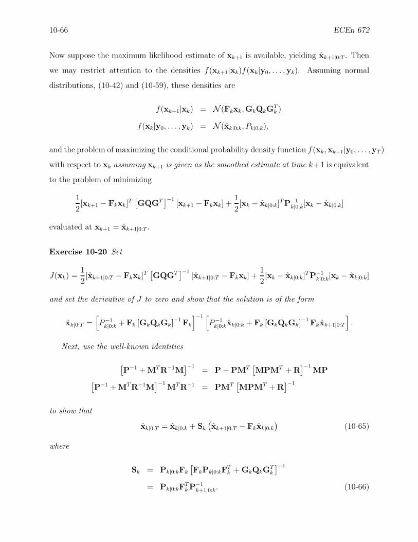
10-66 ECEn 672
Now suppose the maximum likelihood estimate of xk+1 is available, yielding xk+1|0:T . Then
we may restrict attention to the densities f(xk+1|xk)f(xk|y0, . . . ,yk). Assuming normal
distributions, (10-42) and (10-59), these densities are
f(xk+1|xk) = N (Fkxk,GkQkGTk )
f(xk|y0, . . . ,yk) = N (xk|0:k, Pk|0:k),
and the problem of maximizing the conditional probability density function f(xk,xk+1|y0, . . . ,yT )
with respect to xk assuming xk+1 is given as the smoothed estimate at time k+1 is equivalent
to the problem of minimizing
1
2[xk+1 − Fkxk]
T[GQGT
]−1[xk+1 − Fkxk] +
1
2[xk − xk|0:k]
T P−1k|0:k[xk − xk|0:k]
evaluated at xk+1 = xk+1|0:T .
Exercise 10-20 Set
J(xk) =1
2[xk+1|0:T − Fkxk]
T[GQGT
]−1[xk+1|0:T − Fkxk] +
1
2[xk − xk|0:k]
TP−1k|0:k[xk − xk|0:k]
and set the derivative of J to zero and show that the solution is of the form
xk|0:T =[
P−1k|0:k + Fk [GkQkGk]
−1 Fk
]−1 [
P−1k|0:kxk|0:k + Fk [GkQkGk]
−1 Fkxk+1|0:T
]
.
Next, use the well-known identities
[P−1 + MTR−1M
]−1= P −PMT
[MPMT + R
]−1MP
[P−1 + MTR−1M
]−1MTR−1 = PMT
[MPMT + R
]−1
to show that
xk|0:T = xk|0:k + Sk
(xk+1|0:T − Fkxk|0:k
)(10-65)
where
Sk = Pk|0:kFk
[FkPk|0:kF
Tk + GkQkG
Tk
]−1
= Pk|0:kFTk P−1
k+1|0:k. (10-66)

Winter 2009 10-67
Equation (10-65) is the Rauch-Tung-Streibel smoother. Note that it operates in backward
time with xT |0:T , the final filtered estimate, as the initial condition for the smoother.
We next seek an expression for the covariance of the smoothing error, xk|0:T = xk− xk|0:T :
Pk|0:T = Exk|0:T xTk|0:T .
From (10-65),
xk − xk|0:T = xk − xk|0:k − Sk
(xk+1|0:T − Fkxk|0:k
),
or
xk|0:T + Skxk+1|0:T = xk|0:k + SkFkxk+1|0:k.
Multiplying both sides by the transpose and taking expectations yields
Exk|0:T xTk|0:T + Exk|0:T xT
k+1|0:TSTk + SkExk+1|0:T xT
k|0:T + SkExk+1|0:T xTk+1|0:TST
k =
Exk|0:kxTk|0:k + Exk|0:kx
Tk|0:kF
Tk ST
k + SkFkExk|0:kxTk|0:k + SkFkExk|0:kx
Tk|0:kF
Tk ST
k(10-67)
Examining the cross terms of these expressions yields, for example,
Exk|0:T xTk+1|0:T = Exk|0:T [Fkxk|0:T + Gkuk|0:T ]T
= Exk|0:T xTk|0:TFT
k
= EE[xk|0:T xT
k|0:T |y0, . . . ,yT
]FT
k
= EE[xk|0:T |y0, . . . ,yT
]xT
k|0:T
FTk
= E
E [xk|y0, . . . ,yT ]︸ ︷︷ ︸
xk|0:T
−xk|0:T
xT
k|0:T
FTk
= 0.
By a similar argument (or from previous orthogonality results)
Exk|0:kxTk|0:k = 0,
and so all cross terms in (10-67) vanish leaving the expression
Pk|0:T + SkExk+1|0:T xTk+1|0:TST
k = Pk|0:k + SkFkExk|0:kxTk|0:kF
Tk ST
k . (10-68)

10-68 ECEn 672
An important byproduct of the above derivations is the result
Exk|0:T xk|0:T = 0. (10-69)
This result establishes the fact that the smoothed estimation error is orthogonal to the
smoothed estimate, which is equivalent to the claim that the smoothed estimate is the
projection of the state onto the space spanned by the entire set of observations. Thus
smoothing preserves orthogonality.
Continuing,we next, we compute the term
Exk+1|0:T xTk+1|0:T .
To solve for this term, we use the just-established fact that
xk+1 = xk+1|0:T + xk+1|0:T
is an orthogonal decomposition, so
Exk+1xTk+1 = Exk+1|0:T xT
k+1|0:T + Exk+1|0:T xTk+1|0:T
= Exk+1|0:T ExTk+1|0:T + Pk+1|0:T .
Similarly
ExkxTk = Exk|0:kx
Tk|0:k + Pk|0:k.
Furthermore, from (10-44),
Exk+1xTk+1 = FkExkx
Tk FT
k + GkQkGTk .
Substituting these results into (10-68) yields
Pk|0:T + Sk
[Exk+1xk+1 − Pk+1|0:T
]TST
k = Pk|0:k + SkFk
[Exkx
Tk −Pk|0:k
]FT
k STk , (10-70)
or
Pk|0:T + Sk
[Exkxk + GkQkG
Tk − Pk+1|0:T
]TST
k = Pk|0:k + SkFk
[Exkx
Tk −Pk|0:k
]FT
k STk ,
(10-71)
which simplifies to
Pk|0:T = Pk|0:k + Sk
[Pk+1|0:T −GkQkG
Tk − FkPk|0:kF
Tk
]TST
k
= Pk|0:k + Sk
[Pk+1|0:T −Pk+1|0:k
]TST
k . (10-72)
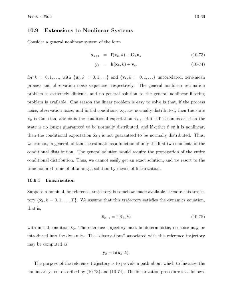
Winter 2009 10-69
10.9 Extensions to Nonlinear Systems
Consider a general nonlinear system of the form
xk+1 = f(xk, k) + Gkuk (10-73)
yk = h(xk, k) + vk, (10-74)
for k = 0, 1, . . ., with uk, k = 0, 1, . . . and vk, k = 0, 1, . . . uncorrelated, zero-mean
process and observation noise sequences, respectively. The general nonlinear estimation
problem is extremely difficult, and no general solution to the general nonlinear filtering
problem is available. One reason the linear problem is easy to solve is that, if the process
noise, observation noise, and initial conditions, x0, are normally distributed, then the state
xk is Gaussian, and so is the conditional expectation xk|j. But if f is nonlinear, then the
state is no longer guaranteed to be normally distributed, and if either f or h is nonlinear,
then the conditional expectation xk|j is not guaranteed to be normally distributed. Thus,
we cannot, in general, obtain the estimate as a function of only the first two moments of the
conditional distribution. The general solution would require the propagation of the entire
conditional distribution. Thus, we cannot easily get an exact solution, and we resort to the
time-honored topic of obtaining a solution by means of linearization.
10.9.1 Linearization
Suppose a nominal, or reference, trajectory is somehow made available. Denote this trajec-
tory xk, k = 0, 1, . . . , T. We assume that this trajectory satisfies the dynamics equation,
that is,
xk+1 = f(xk, k) (10-75)
with initial condition x0. The reference trajectory must be deterministic; no noise may be
introduced into the dynamics. The “observations” associated with this reference trajectory
may be computed as
yk = h(xk, k).
The purpose of the reference trajectory is to provide a path about which to linearize the
nonlinear system described by (10-73) and (10-74). The linearization procedure is as follows.

10-70 ECEn 672
Define the deviation, δxk as the difference between the actual state and the reference state:
δxk = xk − xk. (10-76)
Expanding the dynamics f(xk, k) and the observations h(xk, k)| about the reference trajec-
tory at time k yields
f(xk, k) = f(xk + δxk, k) = f(xk, k) + Fkδxk + higher-order terms.
h(xk, k) = h(xk + δxk, k) = h(xk, k) + Hkδxk + higher-order terms,
where
Fk =∂f(x, k)
∂x
∣∣∣∣x=xk
(10-77)
Hk =∂h(x, k)
∂x
∣∣∣∣x=xk
. (10-78)
Neglecting higher-order terms, we may approximate (10-73) by
xk+1 = f(xk, k) + Gkuk
≈ f(xk, k) + Fkδxk + Gkuk (10-79)
Using (10-73), we rearrange (10-79) to obtain the deviation dynamics equation (replacing
the ≈ with = from here on)
δxk+1 = Fδxk + Gkuk. (10-80)
We see that (10-80) is a linear dynamics model in the deviation variable, δxk. Also, we may
approximate (10-74) by
yk = h(xk, k) + vk
≈ h(xk, k) + Hkδxk + vk. (10-81)
Defining
δyk = yk − yk,
we rearrange (10-81) to obtain the deviation observation equation
δyk = Hkδxk + vk, (10-82)
Winter 2009 10-71
a linear observations model in the deviations.
Once the linearized dynamics and observations equations given by (10-80) and (10-82)
are obtained, we may apply the Kalman filter to this system in δxk in the standard way.
The algorithm consists of the following steps:
1. Obtain a reference trajectory xk, k = 0, 1, . . . , T.
2. Evaluate the partials of f and h at xk; identify these quantities as Fk and Hk, respec-
tively.
3. Compute the reference observations, yk and calculate δyk.
4. Apply the Kalman filter to the linearized model
δxk+1 = Fδxk + Gkuk
δyk = Hkδxk + vk
to obtain the deviation estimates
δxk|0:k (filtered)
δxk|0:T (smoothed).
5. Add the deviation estimates to the nominal trajectory to obtain the trajectory esti-
mates:
xk|0:k = xk + δxk|0:k (filtered)
xk|0:T = xk + δxk|0:T (smoothed).
The approach outlined above is called global linearization, and it has several potential prob-
lems. First of all, it assumes that a reliable nominal trajectory is available, so that the F
and H matrices are valid. But many important estimation problems to not enjoy the lux-
ury of having foreknowledge sufficient to generate a reference trajectory. Also, even if the
F and H matrices are not grossly in error, the approach is predicated on the assumption
that higher-order terms in the Taylor expansion may be safely ignored. It would be highly

10-72 ECEn 672
fortuitous if the nominal trajectory were of such high quality that neither of these concerns
were manifest.
In the general case, however, the development of a nominal trajectory is problematic. In
some special cases it may be possible to generate such a trajectory via computer simulations;
in other cases, experience and intuition may guide it development. Often, however, one may
simply have to rely on guesses and hope for the best. But bad things may happen. The
estimates may diverge, but even if the do not, the results may be suspect because of the
sensitivity of the results to the operating point. Of course, one could perturb the operating
point and evaluate the sensitivity of the estimates to this perturbation, but that would be a
tedious procedure, certainly not possible with real-time applications.
10.9.2 The Extended Kalman Filter
Global linearization about a pre-determined reference trajectory is not the only way to ap-
proach the linearization problem. Another approach is to calculate a local nominal trajectory
“on the fly,” and update it as information becomes available.
Following the timely injunction of Lewis Carrol to “Begin at the beginning, . . . go on until
you come to the end; then stop,” our first order of business will be to get the estimation
process started. We wish to construct a recursive estimator, and regardless of its linearity
properties, we are under obligation to provide the estimator with initial conditions in the
form of x0|−1 and P0|−1, the a priori state estimate and covariance. The state x0|−1 represents
the best information we have concerning the value x0, so it makes sense to use this value as
the first point in the nominal trajectory; that is, to define
x0 = x0|−1,
and use this value to compute the H0 matrix as
H0 =∂h(x, 0)
∂x
∣∣∣∣x=x0|−1
and the deviation observation equation is
δy0 = y0 − h(x0, 0) = y0 − h(x0|−1, 0).
Winter 2009 10-73
Using these values, we may process δy0 using a standard Kalman filter applied to (10-80)
and (10-82). The resulting measurement update is
δx0|0 = δx0|−1 + W0
[δy0 − H0δx0|−1
](10-83)
P0|0 = [I −W0H0]P0|−1, (10-84)
where W0 = P0|−1HT0
[H0P0|−1H
T0 + R0
]−1. But note that x0|−1 fulfills two roles: (a) it is
the initial value of the state estimate, and (b) it is the nominal trajectory about which we
linearize, namely x0. Consequently,
δx0|−1 = x0|−1 − x0 = 0.
Furthermore,
δx0|0 = x0|0 − x0 = x0|0 − x0|−1,
so (10-83) becomes
x0|0 = x0|−1 + W0
[y0 − h(x0|−1, 0)
]. (10-85)
Consequently, (10-85) and (10-84) constitute the measurement update equations at time
k = 0.
Going on, the next order of business is to predict to the time of the next observation
and then update. We will need to compute the predicted state, x1|0, and the predicted
covariance, P1|0. To predict the state, we simply apply the nonlinear dynamics equation:
x1|0 = f(x0|0, 0). (10-86)
To predict the covariance, we need to obtain a linear model, which will enable us to predict
the covariance as
P1|0 = F0P0|0FT0 + G0Q0G
T0 . (10-87)
The question is, what should we use as a nominal trajectory at which to evaluate (10-77)?
According to our philosophy, we should use the best information we currently have about x0,
and this is our filtered estimate. Thus, we take, for the calculation of F0, the value x0 = x0|0.
Using this value, the prediction step at time k = 0 is given by (10-86) and (10-87).

10-74 ECEn 672
The next order of business is, of course, to perform the observation update at time k = 1,
yielding
δx1|1 = δx1|0 + W1
[δy1 − H1δx1|0
]
P1|1 = [I −W1H1]P1|0,
which requires us to employ a reference trajectory x1. Following our philosophy, we simply
use the best information we have at time k = 1, namely, the predicted estimate, so we set
x1 = x1|0. Consequently, δx1|0 = x1|0 − x1 = 0, and δx1|1 = x1|1 − x1|0, which yields
x1|1 = x1|0 + W1
[y1 − h(x1|0, 1)
],
where
W1 = P1|0HT1
[H1P1|0H
T1 + R1
]−1,
with
H1 =∂h(x, 1)
∂x
∣∣∣∣x=x1|0
.
The pattern should now be quite clear. The resulting algorithm is called the extended
Kalman filter, summarized as follows:
Measurement Update
xk+1|k+1 = xk+1|k + Wk+1
[yk+1 − h(xk+1|k, k)
](10-88)
Pk+1|k+1 = [I − Wk+1Hk+1]Pk+1|k, (10-89)
where
Wk+1 = Pk+1|kHTk+1
[Hk+1Pk+1|kH
Tk+1 + Rk+1
]−1, (10-90)
with
Hk+1 =∂h(x, k)
∂x
∣∣∣∣x=xk+1|k
. (10-91)
Time Update
xk+1|k = f(xk|k, k) (10-92)
Pk+1|k = FkPk|kFTk + GkQkG
Tk , (10-93)
Winter 2009 10-75
where
Fk =∂f(x, k)
∂x
∣∣∣∣x=xk|k
. (10-94)
Initialization
The extended Kalman filter is initialized in exactly the same way as is a standard Kalman
filter; namely by supplying the a prior estimate and covariance, x0|−1 and P0|−1, respectively.
Nonlinear Smoothing
The Rauch-Tung-Smoother equations are unchanged from the standard linear filter.
Exercise 10-21 Using the model provided in Section 10.6, rework the problem using the
nonlinear observations vector
yk =
RAE
=
hR(xk)hA(xk)hE(xk)
+ vk
where R denotes the range from a receiver to the vehicle, A denotes the azimuth angle, , and
E is the elevation elevation angle. The mathematical models for these observations are
Range
hR(x) =√
(x − xr)2 + (y − yr)2 + (z − zr)2
∂R
∂x=
1
R[(x − xr), (y − yr), (z − zr)]
where x = [x, y, z] is the position of the vehicle and [xr, yr, zr]T is the position of the radar.
Azimuth
For these calculations we assume that the vectors are resolved into an East-North-Up
coordinate system:
hA(x) = tan−1
[x − xr
y − yr
]
, −π ≤ A ≤ π
∂A
∂x=
1
y − yr[cos2 A,− sin A cos A, 0].
Elevation

10-76 ECEn 672
For these calculations we assume that the vectors are resolved into an East-North-Up
coordinate system:
hE(x) = sin−1
[z − zr
R
]
, −π
2≤ A ≤ π
2
∂E
∂x=
1
R[− sin E sin A, sin E cos A, cos E].
Winter 2009 Bib-1
References
[1] H. D. Brunk. Mathematical Statistics. Blaisdell, Waltham, MA, second edition, 1965.
[2] M. DeGroot. Optimal Statistical Decisions. McGraw-Hill, New York, 1970.
[3] T. S. Ferguson. Mathematical Statistics. Academic Press, New York, 1967.
[4] G. C. Goodwin and R. L. Payne. Dynamic Systems Identification. Academic Press,
New York, 1977.
[5] A. Graham. Kronecker Products and Matrix Calculus with Applicatons. Halsted Press,
New York, 1981.
[6] H. Cramer. Mathematical Methods of Statistics. Princeton Univ. Press, Princeton, NJ,
1946.
[7] C. Howson and P. Urbach. Scientific Reasoning: The Bayesian Approach. Open Court,
La Salle, Illinois, 1989.
[8] A. H. Jazwinski. Stochastic Processes and Filtering Theory. Academic Press, New York,
1970.
[9] R. E. Kalman. A new approach to linear filtering and prediction problems.
Trans. ASME, Ser. D: J. Basic Eng, 82:35–45, 1960.
[10] R. D. Luce and H. Raiffa. Games and Decisions. John Wiley, New York, 1957.
[11] K. V. Mardia, J. T. Kent, and J. M. Bibby. Multivariate Analysis. Academic Press,
New York, 1979.
[12] J. Neveu. Mathematical Foundations of the Calculus of Probability. Holden Day, San
Francisco, 1965.
[13] H. V. Poor. An Introduction to Signal Detection and Estimation. Springer-Verlag, New
York, 1988.

Bib-2 ECEn 672
[14] R. L. Stratonovich. Conditional markov processes. Theor. Probability Appl., 5:156–176,
1960.
[15] P. Swerling. First order error propagation in a stagewise smoothing procedure for
satellite observations. J. Astronautical Sci., 6:46–52, 1959.
[16] H. L. Van Trees. Detection, Estimation, and Modulation Theory, Part I. John Wiley
and Sons, New York, 1968.
[17] H. G. Tucker. A Graduate Course in Probability. Academic Press, New York, 1967.
[18] P. Whittle. Probability via Expectation. Springer-Verlag, New York, 2000. Fourth
Edition.