Embed Size (px)
Citation preview
Detection of very long period seismic signals andacoustic gravity waves generated by large tsunamis:
Application to tsunami warning
Inauguraldissertationzur Erlangung des akademischen Doktorgrades
eingereicht am Fachbereich Geowissenschaften,der Freien Universität Berlin
vorgelegt vonAndriamiranto Raveloson
November 7, 2011
Als Dissertation angenomen vom Fachbereich Geowissenschaftender Freien Universität Berlin.
auf Grund der Gutachtenvon Prof. Dr. Rainer Kindund Prof. Dr. Marco Bohnhoff
Berlin, den 01. November 2011
Statement of AuthorshipThis thesis has been submitted for the degree of Doctor of natural sciences. I, Andriami-ranto Raveloson, hereby declare that:• I am the sole author of this thesis.• I have fully acknowledged and referenced the ideas and work of others, whether
published or unpublished, in my thesis.• I have prepared my thesis specifically for the degree of natural sciences under the
supervision of Prof Rainer Kind at the Freie Universität Berlin.• My thesis does not contain work extracted from a thesis, dissertation or research
paper previously presented for another degree or diploma at this or any other uni-versity.
Eidesstattliche ErklärungDie These ist für den Grad eines Doktors der NaturWissenschafter vorgelegt. Ich, Andri-amiranto Raveloson, erkläre hiermit, dass:• Ich bin der alleinige Urheber dieser These.• Ich habe voll anerkannt und verwiesen die Ideen und die Arbeit der anderen, ob
veröffentlicht oder unveröffentlicht, in meiner Diplomarbeit.• Ich habe meine Diplomarbeit speziell für den Grad eines Doktors der NaturWis-
senschafter, während unter den vorbereiteten Aufsicht von Prof. Rainer Kind an derFreien Universität Berlin.• Meine These enthält keine Arbeit aus einer Diplomarbeit, Dissertation oder Forschungsar-
beit gewonnen zuvor für einen anderen Abschluss oder ein Diplom in dieser oder eineranderen Hochschule vorgestellt.
Andriamiranto Raveloson
Abstract
Tsunamis belong to natural events, which lead to the most devastating global catastro-
phes, although they occur rarely. Because tsunamis caused in recent times large number
of casualties and heavy destruction in wide spread coastal areas, they became the focus
of intensive scientific research. The basis to mitigate casualties due to tsunamis is mainly
continuous monitoring of seismic activity. Since prediction of earthquakes is not possible,
early tsunami warning is the primary goal of related research. So far, direct observations
of tsunamis came only from tide gauges on the shore lines and deep ocean pressure sen-
sors (Deep Ocean Assessment and Reporting of Tsunamis, DART). However, tide gauge
measurements are dominantly influenced by local conditions (shape of the harbor and res-
onances within the harbor) and DART stations have a very poor coverage.
In this thesis, data from seismic and infrasound stations were analyzed in order to see effects
of tsunamis of the great Sumatra-Andaman 2004 and Tohuku-Oki 2011 earthquakes. Data
used are from seismic stations of the Global Seismic Network (GSN) around the Indian and
Pacific oceans and from infrasound stations of the International Monitoring System of the
Comprehensive Test Ban Treaty Organization (IMS/CTBTO). In both data sets, seismic
and infrasound, tsunami signals are observed in the period range of 500to2000s. These
data may add to two new very useful observables for tsunami early warning systems. A
traveling tsunami wave is causing tilting of the ocean bottom and of the coast up to 150km
inland, which is recorded on the horizontal components of broadband seismometers. In the
source region of an earthquake, the bottom of the ocean may be displaced vertically, which
causes vertical displacement of the surface of the sea, and which leads to the generation
of an acoustic gravity wave propagating in the atmosphere. Infrasound signals of the
Sumatra-Andaman and Tohoku-Oki earthquakes have been used successfully to locate the
1
sources of both tsunamis. The epicenter of the Tohoku-Oki tsunami was about 100km to
the south-east of the seismic epicenter, and that of the Sumatra-Andaman event was about
200km to the northwest of the seismic epicenter. The great advantage of this technique is
that infrasound travels with a speed of about 330m/s and the tsunami travels significantly
slower, with a speed of about 200m/s in the deep ocean and much slower in shallow
coastal waters. This technique not only provides the fastest evidence if a tsunami was
indeed generated (which may avoid false alarms), but it also gains additional warning time
and provides basic information on the tsunami source needed for modeling of tsunami
propagation. Implementation of these two new observables into existing tsunami early
warning systems would be relatively easy, because infrasound sensors could be integrated
into seismic stations. Ultra long period seismic observations of tsunamis at coastal stations
would only require some software additions.
2
Zusammenfassung
Tsunamis sind Naturereignisse, die zu den verheerendsten weltweiten Katastrophen gehören,
obwohl sie relativ selten auftreten. Da Tsunamis in letzter Zeit zahlreiche Opfer und
schwere Zerstörungen in groβen Küstenregionen verursacht haben, sind sie Ziel inten-
sivierter Forschungen geworden. Die Grundlage zur Reduzierung von Tsunamiopfern ist ein
kontinuierliches Monitoring der Seismizität. Da eine Erdbebenvorhersage nicht möglich ist,
sind Tsunamifrühwarnungen das primäre Ziel der Forschungen auf diesem Gebiet. Bisher
geschehen direkte Beobachtungen von Tsunamis hauptsächlich durch Messungen des Meer-
esspiegels an Küsten oder durch Drucksensoren in der Tiefsee mit Hilfe von Bojen (Deep
Ocean Assessment and Reporting of Tsunamis, DART). Jedoch werden Küstenpegelmes-
sungen in Häfen dominiert von lokalen Küstenstrukturen und möglichen Resonanzeffekten
und es gibt nur eine relativ geringe Anzahl von DART Stationen im offenen Ozean.
In dieser Dissertation werden Beobachtungen von Tsunamis in seismischen Daten und
in Infrasound Daten der groβen Erdbeben von Sumatra-Andaman 2004 und Tohoku-Oki
2011 analysiert. Die benutzten Daten stammen von den seismischen Stationen des Global
Seismic Network (GSN) im Gebiet des Pazifischen und Indischen Ozeans und von den In-
frasound Stationen des International Monitoring System of the Comprehensive Test Ban
Treaty Organization (IMS/CTBTO). In beiden Datensätzen, den seismischen und den
Infrasound Daten, wurden Signale von Tsunamis im Periodenbereich von 500 bis 2000s
beobachtet. Diese Daten sind neue, möglicherweise sehr nützliche Beobachtungsgröβen für
Tsunamiwarnsysteme. Ein sich ausbreitender Tsunami verursacht Neigungsänderungen
des Meeresbodens und der Küstenregionen bis zu 150km landeinwärts, die auf den Hori-
zontalkomponenten von Breitbandseismometern messbar sind. In der Herdregion von Erd-
beben bewegt sich der Meeresboden möglicherweise vertikal, was zu vertikalen Bewegungen
3
der Meeresoberfläche führt, die wiederum akustische Gravitationswellen in der Atmosphäre
erzeugen. Solche Infrasound Signale der Sumatra-Andaman und Tohoku-Oki Erdbeben
wurden erfolgreich zur Lokalisierung der Herde der Tsunamis benutzt. Das Epizentrum des
Tohoku-Oki Tsunamis wurde ca. 100km südöstlich des seismischen Epizentrums lokalisiert,
und das Epizentrum des Sumatra-Andaman Tsunamis ca. 200km nordwestlich des seis-
mischen Epizentrums. Der groβe Vorteil dieser Methode ist, dass Infrasound sich mit einer
Geschwindigkeit von ca. 330m/s ausbreitet während der Tsunami selbst sich viel langsamer
ausbreitet; mit Geschwindigkeiten von ca. 200m/s in der Tiefsee und mit viel kleineren
Geschwindigkeiten in flachen Küstengewässern. Diese Technik liefert nicht nur die schnell-
sten Hinweise, ob ein Tsunami tatsächlich von einem Erdbeben erzeugt wurde (was falsche
Alarme reduziert), sondern es wird auch zusätzliche Warnzeit gewonnen und wichtige In-
formationen für die Modellierung der Tsunamiausbreitung werden erhalten. Die Einfügung
dieser neuen Beobachtungsgröβen in existierende Tsunamiwarnsysteme sollte relativ leicht
möglich sein, da Infrasoundsensoren sich in existierende seismische Stationen integrieren
lassen. Ultralangperiodische seismische Beobachtungen von Tsunamis an Küstenstationen
würden lediglich Softwareänderungen benötigen.
4
Contents
Abstract 1
Zusammenfassung 3
1 INTRODUCTION 15
1.1 Historical context . . . . . . . . . . . . . . . . . . . . . . . . . . . . . . . . 15
1.2 Present research and motivation . . . . . . . . . . . . . . . . . . . . . . . 16
2 GENERAL INFORMATION ON TSUNAMIS 18
2.1 Physical characteristics of tsunamis . . . . . . . . . . . . . . . . . . . . . . 20
2.1.1 Properties of tsunami . . . . . . . . . . . . . . . . . . . . . . . . . . 20
2.1.2 Tsunami source . . . . . . . . . . . . . . . . . . . . . . . . . . . . . 23
2.1.3 Tsunami propagation . . . . . . . . . . . . . . . . . . . . . . . . . . 25
2.1.4 Tsunami inundation . . . . . . . . . . . . . . . . . . . . . . . . . . 26
2.2 Tsunami warning system . . . . . . . . . . . . . . . . . . . . . . . . . . . . 29
2.2.1 Tsunami registration . . . . . . . . . . . . . . . . . . . . . . . . . . 29
2.2.2 Size of a tsunamis . . . . . . . . . . . . . . . . . . . . . . . . . . . . 29
2.2.3 Tsunami warning system . . . . . . . . . . . . . . . . . . . . . . . . 30
3 Theory of Earth-Ocean-Atmosphere coupling 35
3.1 Seabed-ocean coupling . . . . . . . . . . . . . . . . . . . . . . . . . . . . . 37
5

CONTENTS
3.2 Earth-Atmosphere coupling . . . . . . . . . . . . . . . . . . . . . . . . . . 39
3.2.1 Solid Earth-Atmosphere coupling . . . . . . . . . . . . . . . . . . . 39
3.2.2 Ocean-Atmosphere coupling . . . . . . . . . . . . . . . . . . . . . . 40
3.3 Theoretical analysis of tsunami generation . . . . . . . . . . . . . . . . . . 43
3.3.1 Tsunami gravity wave . . . . . . . . . . . . . . . . . . . . . . . . . 43
3.3.2 Theory of tsunami generation . . . . . . . . . . . . . . . . . . . . . 45
3.4 The response of seismometer to tilt . . . . . . . . . . . . . . . . . . . . . . 47
4 OBSERVATION OF TSUNAMIS 49
4.1 Seismic observation of tsunamis . . . . . . . . . . . . . . . . . . . . . . . . 49
4.1.1 Introduction . . . . . . . . . . . . . . . . . . . . . . . . . . . . . . . 49
4.1.2 The Andaman-Sumatra, Indonesia 2004 tsunami . . . . . . . . . . . 50
4.1.2.1 Observations . . . . . . . . . . . . . . . . . . . . . . . . . 52
4.1.3 The Tohoku, Japan, tsunami 2011 . . . . . . . . . . . . . . . . . . . 52
4.1.3.1 Data . . . . . . . . . . . . . . . . . . . . . . . . . . . . . . 53
4.1.3.2 General descriptions and observations . . . . . . . . . . . 55
4.1.3.3 Discussion . . . . . . . . . . . . . . . . . . . . . . . . . . . 60
4.1.3.4 Conclusion . . . . . . . . . . . . . . . . . . . . . . . . . . 66
4.2 Infrasound observation of tsunamis . . . . . . . . . . . . . . . . . . . . . . 66
4.2.1 Introduction . . . . . . . . . . . . . . . . . . . . . . . . . . . . . . . 66
4.2.2 Infrasound data . . . . . . . . . . . . . . . . . . . . . . . . . . . . . 67
4.2.3 The Andaman-Sumatra, Indonesia 2004 tsunami . . . . . . . . . . . 69
4.2.3.1 Observed data . . . . . . . . . . . . . . . . . . . . . . . . 69
4.2.3.2 Synthetic data . . . . . . . . . . . . . . . . . . . . . . . . 75
4.2.3.3 Interpretation and discussion . . . . . . . . . . . . . . . . 77
4.2.4 The Tohoku, Japan, tsunami 2011 . . . . . . . . . . . . . . . . . . . 79
4.2.4.1 Identification of the infrasound signal . . . . . . . . . . . . 80
6
CONTENTS
4.2.4.2 Location of the infrasound source . . . . . . . . . . . . . . 81
4.2.4.3 Discussion . . . . . . . . . . . . . . . . . . . . . . . . . . . 85
5 DISCUSSION 87
5.1 Observed data . . . . . . . . . . . . . . . . . . . . . . . . . . . . . . . . . . 87
5.2 Synthetic data . . . . . . . . . . . . . . . . . . . . . . . . . . . . . . . . . . 89
5.3 Infrasound generating seismic signal . . . . . . . . . . . . . . . . . . . . . . 92
5.4 Conclusion . . . . . . . . . . . . . . . . . . . . . . . . . . . . . . . . . . . . 93
6 Summary and Outlook 96
Bibliography 99
ACKNOWLEDGEMENT 113
APPENDIX 115
7
List of Figures
2.1 Japanese hieroglyphs pronounced as ’tsu nami’ translated as ’wave in the harbor’ 19
2.2 (top) Phase and group velocity of tsunamis on a flat earth covered by oceans.
(Bottom) Wavelength as a function of wave period (Source: Steven W., Encyclo-
pedia of Physical Science and Technology) . . . . . . . . . . . . . . . . . . . . 22
2.3 Faults system. (a) Strike-slip, (b) Dip-slip, (c) Thrust-dip . . . . . . . . . . . . 23
2.4 Tsunami nucleation by a subducting plate boundary. Rupture zone is shown by
orange line while red star denotes the hypocenter. . . . . . . . . . . . . . . . . 24
2.5 Anatomy of the wave: (a) Wind waves with a circular particle motion. (b)
Tsunamis with elliptic particle motion . . . . . . . . . . . . . . . . . . . . . . 26
2.6 Shoaling amplification factor for ocean waves of various frequencies and source
depth (Source: Encyclopedia of Physical Science and Technology) . . . . . . . . 27
2.7 Tsunami cross section view. Adapted from UNESCO-IOC (Tsunami glossary) . 28
2.8 Prototype of Deep-ocean Assessment and Reporting of Tsunamis (DART)(Source:
http://www.ndbc.noaa.gov/) . . . . . . . . . . . . . . . . . . . . . . . . . . . 31
2.9 Deep-ocean Assessment and Reporting of Tsunamis Station Locations (source:
NOAA) . . . . . . . . . . . . . . . . . . . . . . . . . . . . . . . . . . . . . . 32
2.10 Oceanic ambient noise recorded by hydrophone and horizontal geophone. The
time refers to the temporal position of the spectral frames in the sonogram. (Osler
et al., (1998) . . . . . . . . . . . . . . . . . . . . . . . . . . . . . . . . . . . 33
8
LIST OF FIGURES
2.11 Different components of the German Indonesian Tsunami Early Warning System
(GITEWS) (Source: http://www.gitews.org) . . . . . . . . . . . . . . . . . . . 34
3.1 Schematic diagram showing the solid earth atmosphere coupling, adapted from
Calais, (1998). Vertical displacement of Earth’s surface excites the entire atmo-
sphere up to the ionosphere, and propagate laterally [Artru et al. 2005.] . . . . 36
3.2 Physical interaction between seabed-ocean with horizontal displacement. Light
blue represents the sea-bed excited vertically accompanied by horizontal displace-
ment while the top layer (blue) shows the the sea-surface. The quantity a is the
corresponding response of the sea surface to the excitation from bottom and h0
indicates the ocean depth. h(x, y, t) and η(x, y, t) indicate an arbitrary point at
the sea bottom an on the sea surface respectively [Dutykh et al., 2011]. . . . . . 38
3.3 Comparison of the air (hatched area) above a standing water wave (left), with
pendulum (right), both of period T . The height of the centre of gravity of a
vertical column of the air oscillates similarly to the pendulum (right hand side).
[Posmentier 1967]. . . . . . . . . . . . . . . . . . . . . . . . . . . . . . . . . 41
3.4 Ocean bottom and water surface displacement and coordinate system of tsunami
(not to scale). . . . . . . . . . . . . . . . . . . . . . . . . . . . . . . . . . . 44
3.5 The effect of tilt on inertial seismometers [Clinton, (2004)]. . . . . . . . . . . . 48
4.1 Location map of the seismic station used. The moment tensor solution of the
Sumatra event indicates also its location. . . . . . . . . . . . . . . . . . . . . 50
4.2 Seismic records of the Sumatra-Andaman earthquake of 26 December 2004 sorted
by epicentral distance of the stations. Original unfiltered broadband records in
gray ; long period low pass filtered in black (Fc=1000s). Red boxes indicate the
first wave group of tsunami hitting the island. Zero seconds corresponds to March
11. 2011, 00:00:00. . . . . . . . . . . . . . . . . . . . . . . . . . . . . . . . . 51
9

LIST OF FIGURES
4.3 Location map of the stations used in this study. Star denotes epicenter of the To-
hoku earthquake. Triangles represent seismic stations: black indicate the absence
of a tsunami signal; empty red triangles represent the presence of signal. Tide
gauge stations are indicated by empty brown circle and black squares represent
DART stations. White rectangle with a numbering are the boxes discussed in the
text. . . . . . . . . . . . . . . . . . . . . . . . . . . . . . . . . . . . . . . . 54
4.4 Comparison of seismic data band pass filtered in the frequency range of 1
mHz to 10 mHz with DART data. Location of boxes are shown in figure
4.3. Vertical black lines denote the picked arrival time of the tsunami. δ is
the distance separating seismic and DART stations . . . . . . . . . . . . . 56
4.5 Seismic records band pass filtered in the frequency range of 1 mHz to 10 mHz.
Dashed line denotes the time of the main seismic arrivals. Red rectangle represent
the tsunami wave-group detected and the length is its estimated ringing times. . 59
4.6 Comparison of seismic and tide gauge and DART data in Hawaii. Top: Map
showing the location of seismic, tide gauge and DART stations. Bottom:(a) Seis-
mic data bandpass filtered between 1mHz and 10 mHz.(b) de-tided tide gauge
data.(c) DART data . . . . . . . . . . . . . . . . . . . . . . . . . . . . . . . 61
4.7 Comparison of seismic and tide gauge data in Wake Island. Top: Map showing
the location of seismic and tide gauge stations. Bottom:(a) Seismic data bandpass
filtered between 1mHz and 10 mHz.(b) de-tided tide gauge data. . . . . . . . . 63
4.8 Seismic records (black) band pass filtered [1 to 10 mHz] and calculated marigram
(red) located offshore. δ represents the distance between seismic station and the
imaginary tide gauge station . . . . . . . . . . . . . . . . . . . . . . . . . . . 65
4.9 Infrasound station: (A) Different type of configuration of infrasound station, (B)
End of the pipe (filtering system), (C) Prototype of one array element [www.ctbto.org]. 68
10
LIST OF FIGURES
4.10 Recording of infrasound raw data from four IMS station after summation of all
array elements. . . . . . . . . . . . . . . . . . . . . . . . . . . . . . . . . . . 69
4.11 Left: Filtered data of each element of the infrasound array [BP: 4 - 14 min].
Name of the trace indicates the array element and SUM (red trace) stands for
the summation of all traces. Vertical red line indicates the seismic surface wave
circling the earth and green line are the arrival time of the tsunami. Right:
Configuration of the array. . . . . . . . . . . . . . . . . . . . . . . . . . . . . 71
4.12 Inset: Red inverted triangles indicate seismic stations; infrasound stations are
represented by color coded triangles; The star marks the earthquake epicenter
and white dashed line represents the earthquake rupture track. The red + is the
location of the source of the infrasound signals. . . . . . . . . . . . . . . . . . 72
4.13 Time residual (rms) as a function of sound speed and the latitude along the
rupture track. White circle indicates the solution of the grid search. . . . . . . 73
4.14 Summed infrasound records of each of the four infrasound arrays. The traces
are filtered with an 800 s high pass filter. (A) Tsunami source is assumed at
earthquake epicenter and origin time, traces are shifted according to a reduction
velocity of 330 m/s (zero time). (B) Tsunami source parameters and infrasound
velocity are taken from the caption of Fig. 4.12. Infrasound first arrival times are
given at the traces. . . . . . . . . . . . . . . . . . . . . . . . . . . . . . . . . 74
4.15 US Standard Atmosphere model. (http://science.jrank.org/pages/65157/standard-
atmosphere.html) . . . . . . . . . . . . . . . . . . . . . . . . . . . . . . . . . 76
4.16 Example of synthetic infrasound trace of the great Sumatra-Andaman earthquake.
TS indicates the arrival of tsunami air wave. (Source parameters: Harvard CMT
Double-Couple solution - Earth model: PREM + US Standard Atmosphere) . . . 76
4.17 Three individual components of the infrasound array at Diego Garcia . . . . . . 78
11
LIST OF FIGURES
4.18 Each trace corresponds to the sum of traces in each array at the indicated station
name on the left. Infrasound traces are filtered with a 800s high pass filter. Arrival
times of the signal at each station is indicated on each trace. Zero time on the
plot corresponds to the speed of 290 m/s except for IS53 (dashed line)traveling
with a speed of 356 m/s. . . . . . . . . . . . . . . . . . . . . . . . . . . . . 80
4.19 Grid search technique for the location of the 2011 Tohoku-Oki tsunami.(A) In-
set figure shows the location of the Infrasound array: two black triangles show
the station where signal is absent or very weak wheras colored triangles are the
place where signals are detected.The source of the tsunami obtained from calcu-
lation is shown as a red-white sphere. The seismic epicenter according to the US
Geological Survey is shown as a grey-white beach ball marking the fault orien-
tation. Arrows indicates the vertical displacement of the sea-floor observed by
using GPS/acoustic combination technique [Sato, et al., 2011]. (B) Grid seach
method. White circle corresponds to the location of the tsunami source, isolines
indicate the calculated sound speed in each grid point and the color shows the
time residual between the zero line and the arrival time of the signal. . . . . . . 82
4.20 Enlarged location map of infrasound stations. Circles indicate the possible source
of the tsunami for each station. Coordinates of the tsunami source and average
wave speed of the tsunami are the free parameters in the grid search. The tsunami
source is estimated to be at the intersection of all circles. Solid blue line indicates
the arrival time of the signal recorded at Alaskan station with a speed of 290 m/s
whereas dashed blue line is the same signal with a speed of 356 m/s. . . . . . . 83
4.21 Black trace shows station where there was no signal. Alaskan station (blue) is
taken as reference. The red and green marks indicate speeds of 356 and 290m/sec,
respectively. Zero time corresponds to a speed of 310m/sec. A weak indication
for a signal traveling with a speed of 330m/sec is marked in black at station IS44. 84
12
LIST OF FIGURES
5.1 Comparison of seismic and infrasound records at Diego Garcia.(Different filter
used are written above the trace) A(top): Seismic (red) and infrasound (blue)
data zoomed between the first 30 min. B(bottom): (red) Long period filtered
three-component seismic data. TS indicates the tsunami arrival. (blue) Filtered
infrasound data. IS marks the infrasound arrival. . . . . . . . . . . . . . . . . 88
5.2 : Comparison of theoretical infrasound and seismic traces for the stations at Diego
Garcia. A: High resolution synthetic data of seismic (red) and infrasound (blue).
B:(blue) Filtered synthetic infrasound trace. (red) Theoretical three component
(vertical, radial and transverse) seismic signals for a point source . . . . . . . . 91
5.3 : Comparison of theoretical and observed infrasound and seismic signals at the
arrival time of the infrasound signal at Diego Garcia. . . . . . . . . . . . . . . 93
5.4 C: Seismic and infrasound records of the Sumatra-Andaman earthquake of 26
December 2004 sorted by epicentral distance of the stations. black: Original
unfiltered seismic records; red: long period filtered seismic records; blue: long
period filtered infrasound data. Straight lines with velocity indications for the
different wave types are also given. . . . . . . . . . . . . . . . . . . . . . . . . 95
13

List of Tables
4.1 Observed properties of the tsunami waves generated by the Mw = 9 Japan
earthquake in March 11, 2011. Time indicates the arrival time of the ob-
served tsunami on seismic station. Coastal distance is the distance of the
station from the shore and PGV stands for peak ground velocity i.e. the
maximum amplitude of the first arrival. . . . . . . . . . . . . . . . . . . . . 57
4.2 Infrasound signal observed at IMS stations of the Andaman-Sumatra tsunami. 77
4.3 Infrasound signal observed at IMS stations for the 2011 Tohoku-Oki tsunami. 84
14

Chapter 1
INTRODUCTION
1.1 Historical context
Over the past centuries tsunamis have been considered as one of the most devastating
natural phenomenon on the world. Different geophysical events like landslides, volcanoes,
meteorites can generate tsunamis. Van Dorn (1968) reported that nuclear explosion in the
ocean could generate serious tsunamis. However, the most common cause of tsunamis is
seismic activity in the oceanic area and we should notice that not all big submarine earth-
quakes generate tsunamis. Despite of its rare activity compared to other natural disasters
(earthquakes, hurricanes and tornadoes), tsunamis remain one of the most destructive,
extreme and deadliest hazards. Therefore tsunamis become the central focus of all organi-
zations dealing with natural hazard management. Tsunamis occur more frequently in the
”Ring of Fire” around the Pacific Ocean. More than 1300 events were recorded since 1974
[Soloviev et al. 1986] there. Tsunamis are also observed in the Atlantic Ocean, Caribbean,
Black and Caspian Seas [Nikonov 1997, Dotsenko et al. 2000, Lander et al. 2002] and
the Mediterranean Sea is known to experience about 300 tsunamis. As in the European
coasts, a catastrophic earthquake and tsunami happened in 1755 which destroyed Lisbon,
15
CHAPTER 1. INTRODUCTION
Portugal supposedly to be the largest catastrophe of this kind. Additionally, the fifth large
tsunami which hit Indonesia within a period of 13 years was in Andaman-Sumatra in De-
cember 26th 2004 which generated the largest tsunami in the Indian Ocean. These events
demonstrate that many places can be vulnerable to tsunami hazard. Facing these problem,
tsunami scientists have developed reliable techniques for the early warning system in order
to at least reduce the horrific disaster.
1.2 Present research and motivation
As opposed to earthquake and atmospheric sciences, tsunami science has evolved differ-
ently due to the unavailability until recently of instrumental recordings of tsunami in the
open ocean and its rare and unsystematic occurrence. The only available recordings were
from tide gauges which are known to only represent arrival times and possibly the char-
acter of the first wave polarity. While the basic governing equations have been known for
over 150 years, the measurement of tsunamis in open ocean was only possible in the later
1990s by the National Oceanic and Atmospheric Administration′s (NOAA). The number
of the instrument responded to the excitation of the tsunami has increased in the last few
years. At the initial stage, some of these instruments are not designed to monitor tsunamis.
This allows theorecians to get some reference from the observation of a tsunami and to
validate the state-of-the-art of their model in order to provide a good estimate of the water
level which is very useful for the evacuation of the population in danger. Despite of the
significant progress in tsunami research, the casualty caused by the last tsunami in Japan
triggered a recurring question: what further steps would have been done to improve the
tsunami early warning systems. Thus, this thesis introduces a relatively new method of ob-
serving tsunamis in seismic and infrasound data which could be applied in warning systems.
16
1.2. PRESENT RESEARCH AND MOTIVATION
Therefore, this thesis is structured as follows:
In Chapter 2 we review a general information on tsunamis. Basic knowledge on the physics
of tsunamis is explained as well as the technique of tsunami measurement followed by a
description of existing tsunami warning systems.
In Chapter 3 we introduce the theory of interaction between solid earth, ocean and atmo-
sphere. Here we briefly explain the translation of energy dissipated during the earthquake
accompanied with the vertical displacement of the sea bottom to the ocean and the gener-
ation of tsunamis. The tsunami, in turn, transfers energy to the atmosphere and generate
acoustic gravity waves. In addition, the tilting inferred by loading of ocean gravity waves
in harbors is explained.
Chapter 4 describes the observations of tsunami effect in seismic and infrasound data.
These two geophysical method may be used as a tsunameters.
In Chapter 5 we discuss our results about the possibility of using these new method in
tsunami warning systems and ending up with a concluding remarks in Chapter 6
17

Chapter 2
GENERAL INFORMATION ON
TSUNAMIS
Different places around the world have been identified in the past centuries to be potential
sources of tsunami. When it comes to tsunami hazard, it is worth referring to the historical
tsunami generated by the Lisbon earthquake in 1755. This tsunami has reached countries
as far away as England and even propagated across the Atlantic Ocean to the Caribbean
Isles [Degg & Doornkamp 1994]. The Lisbon tsunami was supposed to be one of the first
well known tsunami which has killed thousands of people [Pacific Disaster Center report].
The city of Lisbon was severely destroyed and most of the coastal towns and villages were
damaged. The intensity of the event was accurately illustrated by several painters. Seis-
mologists tried to reconstruct the signal and estimated the magnitude of the earthquake
to be 9.0 Mw (USGS).
In the 1950s the destructive oceanic waves were still a very complicated puzzle for scientists
and considered as a mysterious event by the whole population who had experienced such
a phenomenon. The word ”tsunami” is the pronunciation of two Japanese hieroglyphs
18
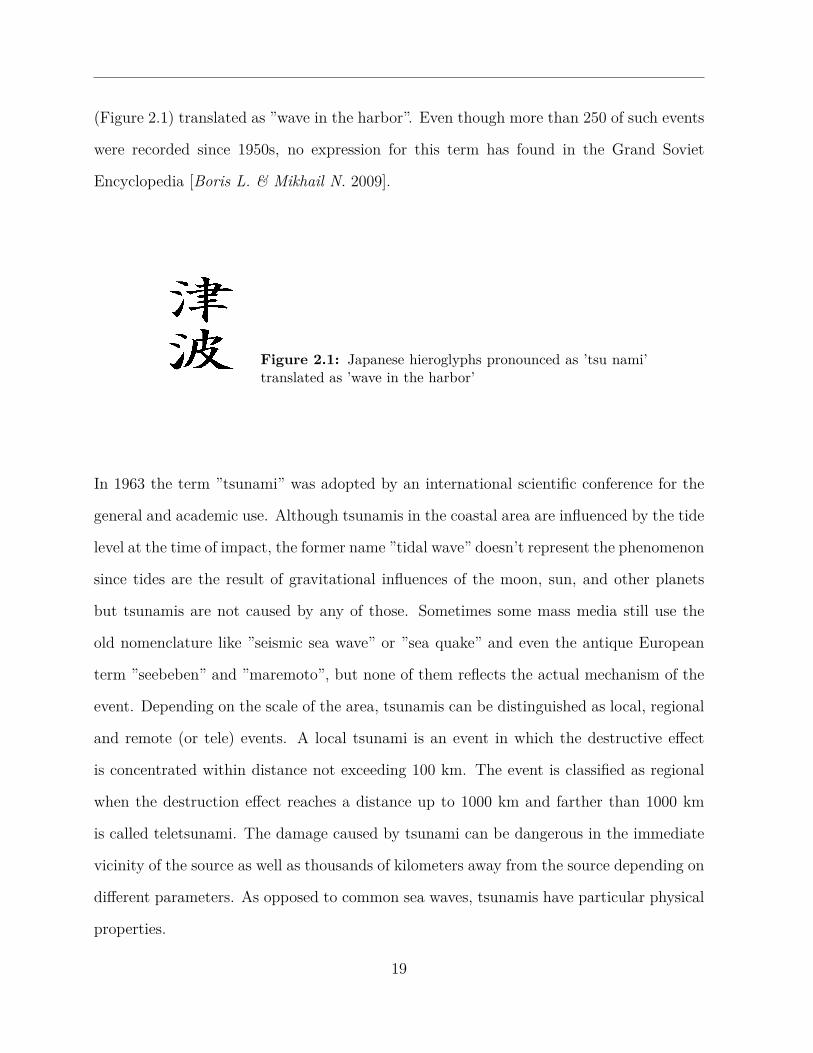
(Figure 2.1) translated as ”wave in the harbor”. Even though more than 250 of such events
were recorded since 1950s, no expression for this term has found in the Grand Soviet
Encyclopedia [Boris L. & Mikhail N. 2009].
Figure 2.1: Japanese hieroglyphs pronounced as ’tsu nami’translated as ’wave in the harbor’
In 1963 the term ”tsunami” was adopted by an international scientific conference for the
general and academic use. Although tsunamis in the coastal area are influenced by the tide
level at the time of impact, the former name ”tidal wave” doesn’t represent the phenomenon
since tides are the result of gravitational influences of the moon, sun, and other planets
but tsunamis are not caused by any of those. Sometimes some mass media still use the
old nomenclature like ”seismic sea wave” or ”sea quake” and even the antique European
term ”seebeben” and ”maremoto”, but none of them reflects the actual mechanism of the
event. Depending on the scale of the area, tsunamis can be distinguished as local, regional
and remote (or tele) events. A local tsunami is an event in which the destructive effect
is concentrated within distance not exceeding 100 km. The event is classified as regional
when the destruction effect reaches a distance up to 1000 km and farther than 1000 km
is called teletsunami. The damage caused by tsunami can be dangerous in the immediate
vicinity of the source as well as thousands of kilometers away from the source depending on
different parameters. As opposed to common sea waves, tsunamis have particular physical
properties.
19

CHAPTER 2. GENERAL INFORMATION ON TSUNAMIS
2.1 Physical characteristics of tsunamis
Tsunamis are considered as long period gravitational waves in the ocean.While propa-
gating, not only does the subsurface layer move but also the entire height of the water
column becomes involved. In general the size of teleseismic tsunami is proportional to the
magnitude of the earthquake i.e. the size of the tsunami increases with the magnitude
of the earthquake. However, the magnitude of the earthquake and its location alone are
not enough to predict an occurrence of a tsunami. The November 2002 earthquake in
the Simeulue island with a magnitude of 7.6 Ms did not generate any significant tsunami
despite its location under water and the strong ground shaking generated. Conversely,
the Java earthquake in 2006 with 7.2 Ms caused a remarkable tsunami. Note that both
sources are on thrusting fault system. Therefore, different parameters must be involved to
study and describe tsunami effects from the generation through propagation and up to the
inundation phase. These phases are described in the following paragraphs.
2.1.1 Properties of tsunami
Tsunamis are mainly known as a deformation of the sea surface excited by any undersea
events. Due to the complexity of the actual phenomenon, some simplifications are needed
in order to determine the basic features of the physical process of the wave. For the case
of tsunamis generated by submarine landslide, for instance, Tinti et al. (2001) simplified
the source by considering a small-height slide which permits them to use linear theory of
the wave motion related to a shallow-water model.
As for the tsunami earthquakes, the amplitude of the tsunami and the seismic moment are
generally considered to be linearly dependent [Kanamori 1972;Abe 1973]. Although the
nonlinear effect is considered to be negligible, the general feature of the wave obtained from
20
2.1. PHYSICAL CHARACTERISTICS OF TSUNAMIS
these assumptions, for both near and far fields, provides an ample understanding of the
physical characteristics of the tsunami. In its simplified form, tsunami is then considered
as surface gravity waves of an incompressible flat oceanic layer with a constant thickness
(depth) h over the rigid half space. The phase c(ω) and group u(ω) velocity of the tsunami
are governed by the following equations:
c(ω) =
√g tanh[k(ω)h]
k(ω)
u(ω) = c(ω)[
12 + k(ω)h
sinh[2k(ω)h]
] (2.1)
where, g is the acceleration of gravity (g=9.8 m/s2) and k is the wavenumber associated
with the frequency ω.
The wavenumber is linked to wavelength by:
λ(ω) = 2πk(ω) (2.2)
then,
(1)+(2) →
c(ω) =
√g tanh
[2πλ(ω)h
]λ(ω)
2π
u(ω) = c(ω)[
12 + 2πh
λ(ω)sinh[
2πλ(ω)h
]] (2.3)
Equation 2.3 illustrates that tsunamis of different wavelengths travel at different speeds.
Consequently tsunamis are considered to be dispersive waves. While approaching the
coast tsunamis slow down, because of depth effect, and amplitudes increase. Under these
conditions, tsunamis exhibit not only frequency dispersion but also amplitude dispersion.
Variations of phase and group velocities as a function of period are illustrated in Figure
2.2. In order to generate a tsunami, a submarine earthquake must move vertically a con-
siderable area. For the case of Sumatra 2004, for instance, the fault width across E-W
21
CHAPTER 2. GENERAL INFORMATION ON TSUNAMIS
Figure 2.2: (top) Phase and group velocity of tsunamis on a flat earth covered by oceans.(Bottom) Wavelength as a function of wave period (Source: Steven W., Encyclopedia of PhysicalScience and Technology)
22
2.1. PHYSICAL CHARACTERISTICS OF TSUNAMIS
Figure 2.3: Faults system. (a) Strike-slip, (b) Dip-slip, (c) Thrust-dip
profile is estimated to be 120 km [Meltzner et al. 2006]. Assuming that the deformation
at sea bottom is translated to the sea surface, we could determine the dimension of the
displaced sea floor by measuring the wavelength of the observed wave at the sea surface.
Figure 2.2 (bottom panel) shows that the wavelength of a tsunami can be as large as 500
km so does the size of the source area.
For a very long wavelength (kh → 0 ) the phase velocity is c(ω)=u(ω)=√gh. This demon-
strates the absence of dispersion in the very long wavelength represented by flat curve on
the left hand side in Figure 2.2 (top panel). When it comes to the short wavelength (kh
→ ∞) phase velocity becomes c(ω)=2u(ω)=√
gλ(ω)2π and waves propagate with dispersion.
2.1.2 Tsunami source
Tsunamis are mainly generated by three geophysical events:
Volcanic eruption can cause tsunamis. The case of the 1883 Krakatoa event is one of
the relevant examples. There was a significant damage and considerable loss of lives but
the mechanism which triggered the tsunamis was not very clear whether by the explosion
[Yokoyama 1981; 1987], by caldera collapse [Verbeek 1885; Francis 1985; Sigurdsson et al.
1991] or by a pyroclastic flow [Self & Rampino 1981].
23
CHAPTER 2. GENERAL INFORMATION ON TSUNAMIS
Figure 2.4: Tsunami nucleation by a subducting plate boundary. Rupture zone is shown byorange line while red star denotes the hypocenter.
Submarine landslides like the one in Aitape, Papua New Guinea in 1998 can a generate
local tsunami which swept out 25 km along the coast with maximum water wave of 15 m
above sea level [Watts P. et al. 2001].
But the most frequent sources of large tsunamis are submarine earthquakes with a mo-
ment magnitude stronger than 7.0 and a focal depth less than 50 km. The hypocenter is
commonly on the rupture along fault lines where two plates are moving against each other.
There are three main faulting systems: strike-slip system, dip-slip system and thrusting
fault system (Figure 2.3).
Normally, a tsunami will be formed only if an earthquake causes vertical displacement of
the sea floor and the source area is three times greater than the ocean depth at the source.
As an example, the 7.9 Mw earthquake in 1906, located at 3.2 km west of San Francisco
(37.75 ◦N, 122.55 ◦W) in the Pacific Ocean with a depth of only 8km [USGS], did not gen-
erate a tsunami because the motion on the fault was strike-slip (Figure 2.3a) motion with
no vertical displacement. Tsunamis only occur if the earthquake source is dip-slip or thrust
24
2.1. PHYSICAL CHARACTERISTICS OF TSUNAMIS
type(Figure 2.3b, c). Because of this, most tsunamis are generated by earthquakes that
occur near subduction boundaries of plates, usually along oceanic trenches.
Due to a driving force of plate tectonics, two plates converge and one slides beneath the
other in a subduction zone. The average speed of this displacement is in the order of
centimeters per year. The main thrust fault is locked during the interseismic time period
(Figure 2.4). The accumulation of stress on the inter-plate contact in a subducting litho-
sphere is associated with crustal deformation usually pronounced by the bending of the
slab.
A none strike-slip earthquake results in a sudden vertical displacement of the ocean bottom
[Bilham et al. 2005, Ji 2005, Fine et al. 2005, Song et al. 2005 and Heki et al. 2006].
Because the ocean is an incompressible and non viscous fluid, the upward movement of the
sea floor causes a vertical deformation of the sea surface. The higher the vertical displace-
ment, the bigger the tsunami amplitude at source becomes . After the generation of the
tsunami, the gravity force tends to restore equilibrium causing propagation of the waves
known as ”tsunami” which can travel thousands of kilometers.
2.1.3 Tsunami propagation
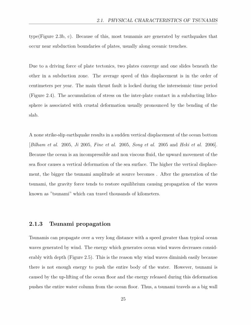
Tsunamis can propagate over a very long distance with a speed greater than typical ocean
waves generated by wind. The energy which generates ocean wind waves decreases consid-
erably with depth (Figure 2.5). This is the reason why wind waves diminish easily because
there is not enough energy to push the entire body of the water. However, tsunami is
caused by the up-lifting of the ocean floor and the energy released during this deformation
pushes the entire water column from the ocean floor. Thus, a tsunami travels as a big wall
25
CHAPTER 2. GENERAL INFORMATION ON TSUNAMIS
Figure 2.5: Anatomy of the wave: (a) Wind waves with a circular particle motion. (b) Tsunamiswith elliptic particle motion
of water towards the shore at relatively constant speeds from sea bottom to surface and
particles move in an elliptical trajectory.
2.1.4 Tsunami inundation
After traveling through the ocean, tsunamis move from deep to shallow water. In general,
ocean waves break far offshore but this condition varies with the type of the wave. Typical
wind waves break near the shore. Waves generated by large explosions or small asteroids in
the ocean break at the continental shelf. However, typical waves from undersea earthquake
don’t break. This is known as ”Van Dorn Effect”.
Towards the shore, water depth decreases and tsunamis slow down. Coming from the deep
ocean with a speed of a jet airplane (≈ 800km/h), the tsunami moves a large amount of
water which will pile up on the continental shelf. Thus, while moving toward the shore
the wave amplitude grows up to a large swell because the shelf is small compared to the
distance between crests. This amplification of the wave is given by the shoaling factor, S,
26

2.1. PHYSICAL CHARACTERISTICS OF TSUNAMIS
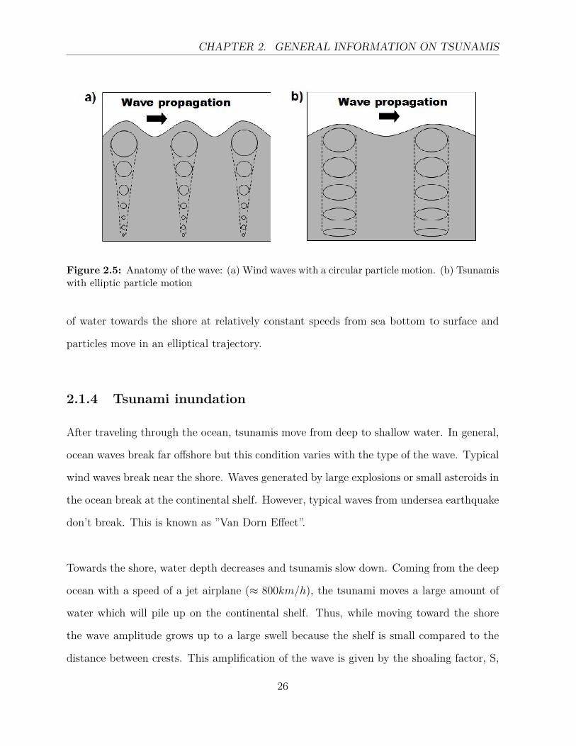
Figure 2.6: Shoaling amplification factor for ocean waves of various frequencies and sourcedepth (Source: Encyclopedia of Physical Science and Technology)
27
CHAPTER 2. GENERAL INFORMATION ON TSUNAMIS
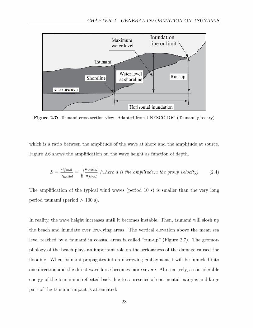
Figure 2.7: Tsunami cross section view. Adapted from UNESCO-IOC (Tsunami glossary)
which is a ratio between the amplitude of the wave at shore and the amplitude at source.
Figure 2.6 shows the amplification on the wave height as function of depth.
S = afinalainitial
=√uinitialufinal
(where a is the amplitude,u the group velocity) (2.4)
The amplification of the typical wind waves (period 10 s) is smaller than the very long
period tsunami (period > 100 s).
In reality, the wave height increases until it becomes instable. Then, tsunami will slosh up
the beach and inundate over low-lying areas. The vertical elevation above the mean sea
level reached by a tsunami in coastal areas is called ”run-up” (Figure 2.7). The geomor-
phology of the beach plays an important role on the seriousness of the damage caused the
flooding. When tsunami propagates into a narrowing embayment,it will be funneled into
one direction and the direct wave force becomes more severe. Alternatively, a considerable
energy of the tsunami is reflected back due to a presence of continental margins and large
part of the tsunami impact is attenuated.
28
2.2. TSUNAMI WARNING SYSTEM
2.2 Tsunami warning system
2.2.1 Tsunami registration
In general, tsunamis are supposedly generated by submarine earthquakes. With the help
of the global or with local seismographic networks, seismologists are able to locate the
earthquake and determine its magnitude. Knowing the origin time of the earthquake, one
can estimate the probable arrival time of tsunami at shore. Besides, tide gauge has been
used to register the sea level anomalies in the coastal area since in the 1900s and can be
used to measure the passage of tsunami at shore. However, neither earthquake parameters
nor coastal tide gauges provide data that allow accurate prediction of tsunami at different
places. Firstly because strong submarine earthquake is not logically accompanied by a
large tsunami and sometimes moderate earthquake can generate destructive waves to the
coast. Secondly tide gauge provides the direct height of the sea at a particular coastal
location but the tsunami is significantly altered by local bathymetry and harbor shapes.
This might limit the use of these two techniques for tsunami warning system.
2.2.2 Size of a tsunamis
Even before the existence of instrumental record for tsunamis several attempts were made
to quantify tsunamis. The first tsunami magnitude scale was known as ”Imamura-Ida
scale” m which is the log base 2 of the maximum run-up height in meters [Ida et al., 1967].
This scale was extended by Hatori, (1979) by including far-field tsunami data and the
effect of distance. He constructed a diagram in log-log scale. This diagram shows a decay
R−1/2 of tsunami height with distance which is theoretically predicted for non-dispersive
waves traveling a long distance [Comer 1980 ] .Soloviev (1970), changed the Imamura-Iida
scale and came up with a new intensity scale. In his formula, he used the mean tsunami
29
CHAPTER 2. GENERAL INFORMATION ON TSUNAMIS
height and added a factor√
2 in the logarithm. For the tsunami magnitude Mt, Abe (1988)
defined a quantity similar to that used since the 1960s in seismology for the measurement
of the surface wave earthquake magnitude (see equation 2.5):
Mt = a logH + b log ∆ +D (2.5)
where H (m) is the maximum single (crest or trough) amplitude of tsunami; ∆ (Km) is
the distance epicenter-tide gauge; a, b and D are constants.
2.2.3 Tsunami warning system
Until recently all ideas of monitoring the evolution of waves in open ocean like tsunamis
were based exclusively on coastal measurement. This idea was criticized by Jacques and
Soloviev (1971) as they introduced a technique of measuring waves in the deep ocean to
avoid any influence of the coast. However, the first prototype of such an instrument came
only out 24 years later.
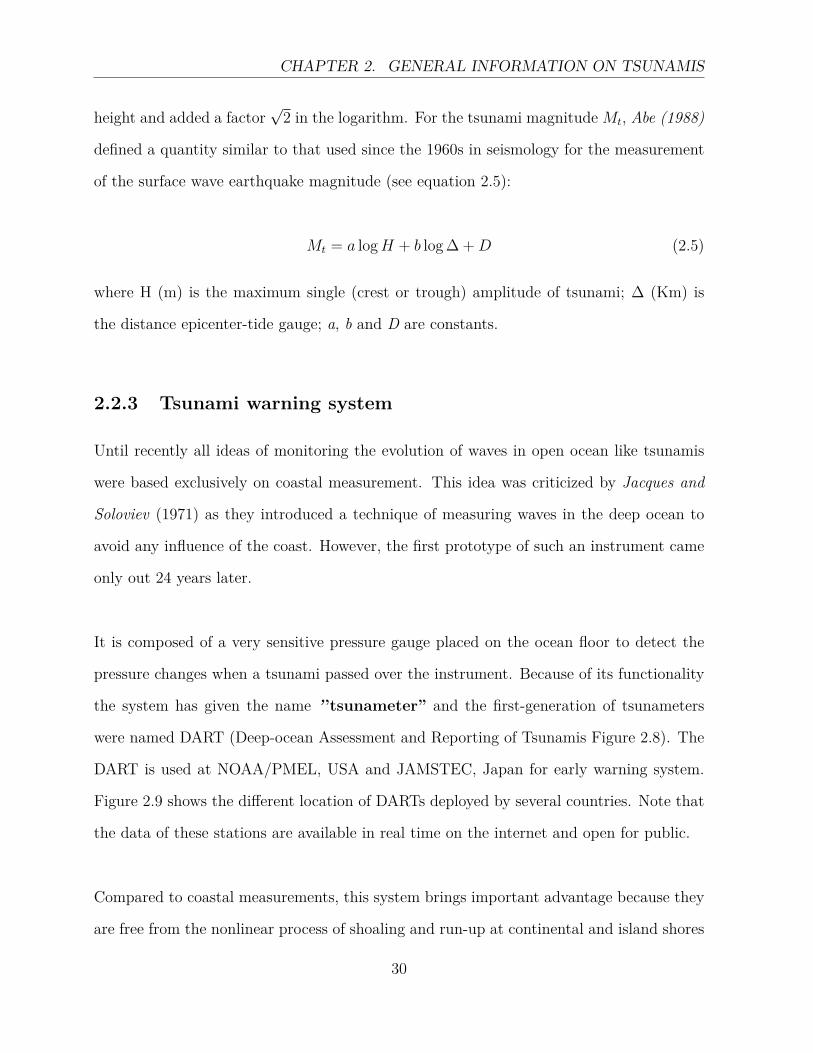
It is composed of a very sensitive pressure gauge placed on the ocean floor to detect the
pressure changes when a tsunami passed over the instrument. Because of its functionality
the system has given the name ’’tsunameter” and the first-generation of tsunameters
were named DART (Deep-ocean Assessment and Reporting of Tsunamis Figure 2.8). The
DART is used at NOAA/PMEL, USA and JAMSTEC, Japan for early warning system.
Figure 2.9 shows the different location of DARTs deployed by several countries. Note that
the data of these stations are available in real time on the internet and open for public.
Compared to coastal measurements, this system brings important advantage because they
are free from the nonlinear process of shoaling and run-up at continental and island shores
30
2.2. TSUNAMI WARNING SYSTEM
Figure 2.8: Prototype of Deep-ocean Assessment and Reporting of Tsunamis (DART)(Source:http://www.ndbc.noaa.gov/)
31

CHAPTER 2. GENERAL INFORMATION ON TSUNAMIS
Figure 2.9: Deep-ocean Assessment and Reporting of Tsunamis Station Locations (source:NOAA)
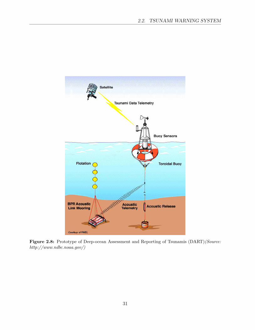
[Okal et al. 2007]. However the availability of such kind of station is very limited because
of their cost and high maintenance requirements. As an example, the cable connecting
the sensor to the buoy is sometimes mixed up with fisher boats and gets destroyed. There
is also a problem of acoustic interference with ships and biological noise [Gonzalez et al.
1998]. Figure 2.10 shows an example of different ambient noise recorded in Emerald Basin
during an experiment conducted by Osler et al. (1998).
For any natural disaster, it is important to create an automated system of continuous obser-
vation in order to provide timely and reliable warning. In the history of tsunami warning,
the system evolves gradually with the impact of destructive events and the progress of tech-
nology. Thomas Jaggar, founder of the Hawaiian Volcano Observatory (HVO), was the
first person who issued a tsunami warning. He warned people of the possibility of big ocean
wave in Hilo, Hawaii after the 1923 Kamchatka earthquake but very few people believed
him. The tsunami warning became official only after the 1946 tsunami in the Aleutian
32
2.2. TSUNAMI WARNING SYSTEM
Figure 2.10: Oceanic ambient noise recorded by hydrophone and horizontal geophone. Thetime refers to the temporal position of the spectral frames in the sonogram. (Osler et al., (1998)
Islands. The center at Hawaii was established to watch the possibility of tsunami at the
west coast of the US and Alaska. In 1960 the Chilean earthquake generated a tsunami and
places as far away as Japan were devastated. This event increased the efforts by the center
and cooperation was established between PTWS, USA and JMA, Japan [NOOA/PTWS].
The devastating Sumatra event in December 2004 showed that the role of the PTWC was
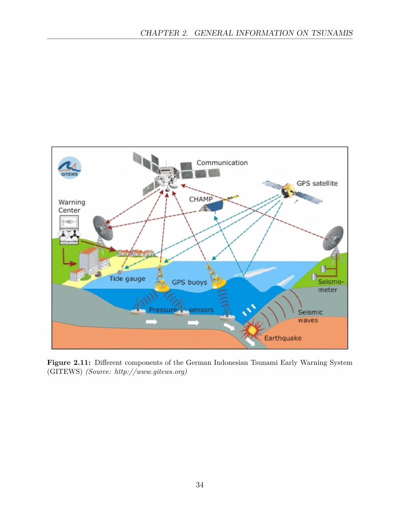
limited. In 2005 the German and Indonesian governments agreed to coordinate efforts to
build up an effective tsunami warning system in the Indian Ocean. The German Indonesian
Tsunami Early Warning System (GITEWS) was established and the new system uses
different variety of sensors like seismometers, GPS instruments, tide gauges and GPS-
buoys as well as ocean bottom pressure sensors Figure 2.11. Because Indonesia is located
along subduction zones the principal sources of tsunami in this region are local submarine
earthquakes. Thus, the project aims to provide new procedures for the fast and reliable
determination of strong earthquakes parameters by integrating available data from different
sensors.
33
CHAPTER 2. GENERAL INFORMATION ON TSUNAMIS
Figure 2.11: Different components of the German Indonesian Tsunami Early Warning System(GITEWS) (Source: http://www.gitews.org)
34
Chapter 3
Theory of Earth-Ocean-Atmosphere
coupling
Frequently people assume for simplicity that the solid earth is decoupled from its atmo-
sphere. Seismologists, for instance, consider the Earth’s solid surface as a free surface
whereas atmospheric scientists assume it as rigid surface. This is reasonably acceptable
if we consider the high density contrast at the surface boundary. However, coupling does
exist between these two media and provides many benefits which may include also the
analysis of mechanisms involved in tsunami generation. On one hand the solid earth is ex-
cited continuously by its atmosphere with acceleration amplitude of about 0.3-0.5 nanogals
in the fundamental modes between 2 and 7 mHz [Nishida et al. 2000; Rhie et al. 2004].
The atmosphere also vibrates due to an earthquake [Lognonne et al. 1998].
For the case of tsunamis, the water layer is excited by the dynamic seabed displacement
caused by seismic faulting and transfers the energy to the sea surface. In turn, it generates
an impulsive signal into the atmosphere and waves can propagate to a very long distance.
Conversely, perturbation in the atmosphere generates a signal in the solid earth. Harkrider
35
CHAPTER 3. THEORY OF EARTH-OCEAN-ATMOSPHERE COUPLING
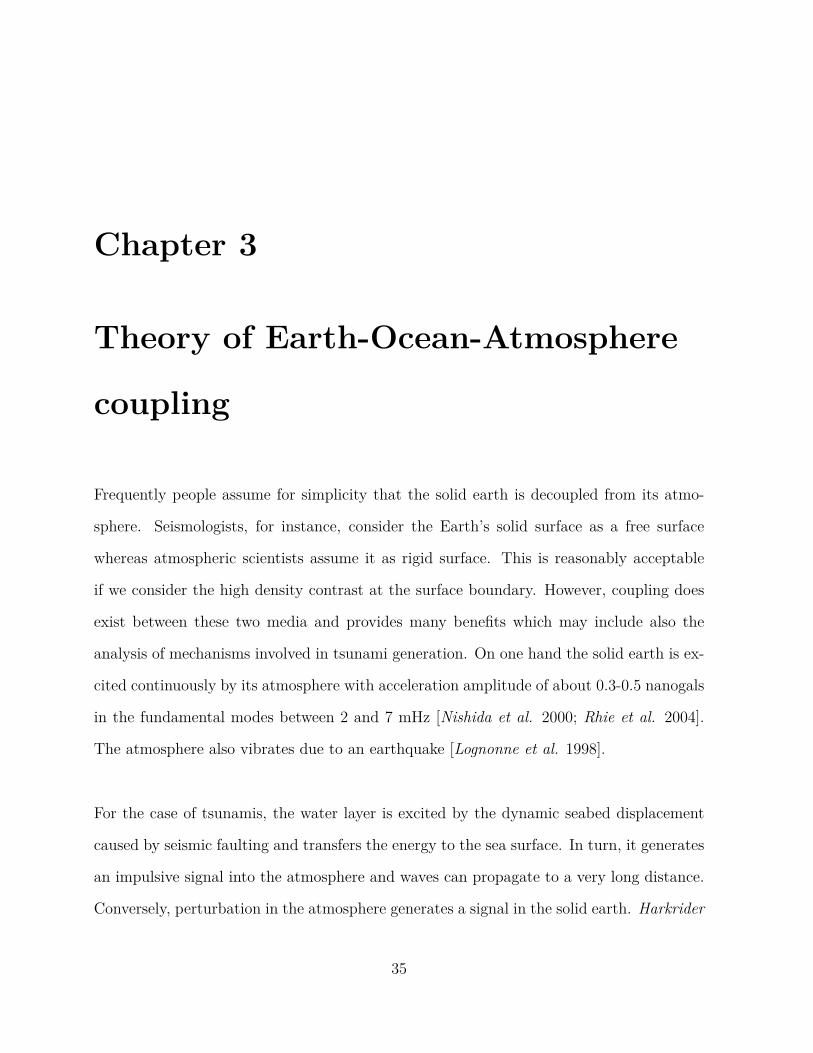
Figure 3.1: Schematic diagram showing the solid earth atmosphere coupling, adapted fromCalais, (1998). Vertical displacement of Earth’s surface excites the entire atmosphere up to theionosphere, and propagate laterally [Artru et al. 2005.]
36
3.1. SEABED-OCEAN COUPLING
and Press (1967) reported that the energy produced by an explosion in the atmosphere
can be transferred to the ocean in an efficient manner and can trigger long period seismic
waves in the solid earth [see also Widmer & Zurn, 1992]. However the coupling is generally
greater over continents than over oceans and the difference may reach the equivalent of 0.5
magnitude units [Harkrider et al. 1973]. Figure 3.1 illustrates different phenomena which
interact with the atmosphere. As mentioned in the previous chapter, the main source of
a tsunamis is an underwater earthquake. In this chapter, the first two sections will review
the state-of-the-art regarding interaction between solid earth, ocean and atmosphere. Then
we will emphasize the necessary condition for an earthquake to generate a tsunami and
the last section will discuss the effect of tilting on seismometers.
3.1 Seabed-ocean coupling
In spite of the progress of science and technology, there are still many open questions in
tsunami research. Since the last few decades theoretical-numerical techniques have become
available to make the computation of tsunamis possible. This has much improved the un-
derstanding of the physical mechanism involved in tsunami generation. Tsunami modelers
need to have detailed knowledge about the source generation which is one of the required
initial conditions before the propagation of the wave in deep ocean and its run-up can be
calculated [Nosov 1998].
For submarine earthquake an accurate prediction of tsunami heights depends on having a
good estimation of the initial sea surface disturbance caused by a submarine earthquake.
This mechanism is basically indicated as the coupling between seabed and the ocean.
In the past studies, different theories have been proposed. Initially Kajiura (1963) formu-
37
CHAPTER 3. THEORY OF EARTH-OCEAN-ATMOSPHERE COUPLING
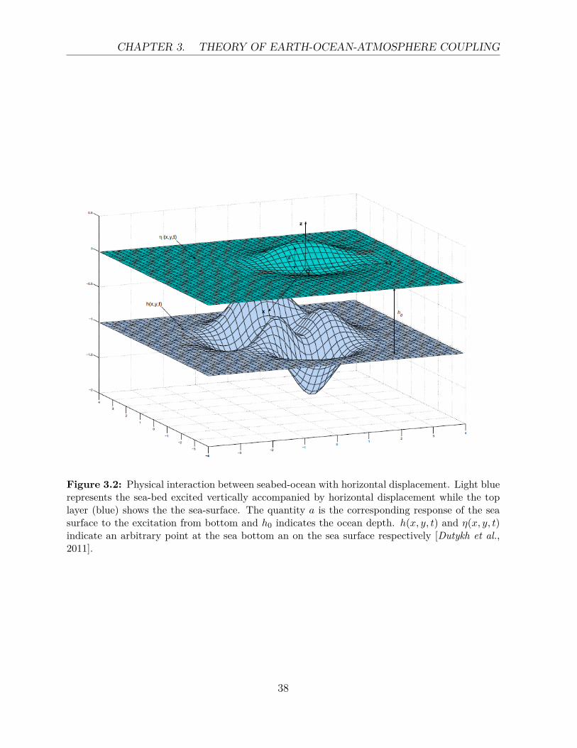
Figure 3.2: Physical interaction between seabed-ocean with horizontal displacement. Light bluerepresents the sea-bed excited vertically accompanied by horizontal displacement while the toplayer (blue) shows the the sea-surface. The quantity a is the corresponding response of the seasurface to the excitation from bottom and h0 indicates the ocean depth. h(x, y, t) and η(x, y, t)indicate an arbitrary point at the sea bottom an on the sea surface respectively [Dutykh et al.,2011].
38
3.2. EARTH-ATMOSPHERE COUPLING
lated that the water wave generation is caused by seabed deformation. Kajiura, (1970)
discussed the energy exchange between seabed and the water. To study the tsunami
generation Yamashita and Sato, (1974) evaluated effects of fault parameters on tsunami
amplitude. In these studies only the static contribution of the seabed displacement is
considered with a strong coupling between seabed and ocean. To overcome this problem
Omachi et al. (2001) and Wang et al. (2004) demonstrate that seabed-wave coupling is
weak. Consequently, the motion of sea water is influenced by that of the seabed, but the
motion of the seabed can be assumed not to be influenced by that of the seawater. More
recently, Dutykh et al. (2011) discussed the effect of the horizontal coseismic displacement
on the tsunami generation, see Figure 3.2. Horizontal motion of the sea bottom is not very
effective from the stand point of tsunami generation. When the sea bottom is inclined,
due to the presence of topography, the effect can be assumed to be similar to the case of
landslide. For the case of landslides the interaction seabed-ocean depends on the volume
of sliding body. Only limited part of the potential energy released by the landslide is
transferred to wave energy . The length of the landslide influences both the wavelength
and the surface elevation while the thickness and acceleration of the landslide as well as
the wave speed determine the surface elevation [Harbitz et al. 2006].
3.2 Earth-Atmosphere coupling
3.2.1 Solid Earth-Atmosphere coupling
Air-ground coupling phenomena have been among the routine observations of many re-
searchers in geoscience. Yuen et al. (1969) and Weaver et al. (1969) reported atmospheric
disturbances following a large earthquake. Several scientists have demonstrated that shal-
low events in the solid Earth can produce impulsive vertical displacements of the surface
that changes the pressure in the atmosphere. Afraimovich et al. (2001) investigated the
39

CHAPTER 3. THEORY OF EARTH-OCEAN-ATMOSPHERE COUPLING
acoustic shock waves in the atmosphere induced by earthquakes. Calais, et al.(1997) and
Fitzgerald (1996) demonstrated that perturbations caused by mine blasts reach the iono-
spheric layer. Blanc (1985) and Ducic et al. (2003) studied an ionospheric impulsive
anomaly associated with Rayleigh waves. Using normal modes approach used in seismol-
ogy, Watada (1995) also mentioned that resonant coupling occurs between the solid Earth
and the atmosphere when their modes overlap in frequency-wavenumber domain. Some
observations of long period surface waves will be discussed later.
3.2.2 Ocean-Atmosphere coupling
Similarly to shallow earthquakes, ocean swelling also can be source of excitation of the
atmosphere. However, the interaction of ocean waves with the atmosphere is not linear
[Arendt and Fritts 2000; Garces et al. 2002 ] due to the temporal and spatial variation
in the structure of the atmosphere [Kulichkov et al. 2004 ]. Since 1996, permanent ob-
servation of the atmosphere becomes possible thanks to the global infrasound network
of the International Monitoring System (IMS) for the compliance of the Comprehensive
Nuclear-Test-Ban Treaty (CTBT). Continuous monitoring of infrasonic waves at different
IMS stations reveals the existence of atmospheric-ocean coupling. Le Pichon et al. (2004)
and Willis et al. (2004), for instance, detected a dominant source of infrasonic waves
caused by ocean swells. They concluded that the infrasonic waves generated by ocean sur-
face waves are characterized by the quasi-permanent infrasonic spectral peak of 0.2 Hz. To
explain the infrasonic signal called ”microbaroms”, which is generated by standing water
waves associated with marine storms, Posmentier (1967) used the theory of the origin of
microseisms developed by Longuet-Higgins (1950). This theory is based on the oscillations
of the center of gravity of the air above the ocean surface on which the standing waves
appear: Posmentier (1967) considers a model of incompressible air of density ρ0 bounded
below by a surface perturbed by two sinusoidal wave trains identical in period T , wave-
40
3.2. EARTH-ATMOSPHERE COUPLING
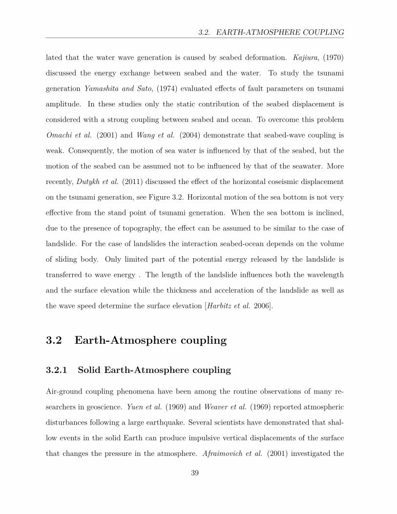
length λ0, and amplitude a, but traveling in opposite directions . This movement creates
a standing wave which excites the air above and the oscillation of the center of gravity of
the vertical column of the air is similar to that of a pendulum (Figure 3.3). Therefore, the
standing wave in the water produces a vertical propagating acoustic wave in the air above.
Figure 3.3: Comparison of the air (hatched area) above a standing water wave (left), withpendulum (right), both of period T . The height of the centre of gravity of a vertical column ofthe air oscillates similarly to the pendulum (right hand side). [Posmentier 1967].
The governing equation of the standing wave is:
η = 2a cos(k0x) cos(ωt), where ω = 2πT
and k0 = 2πλ0
and η is the surface height. (3.1)
41
CHAPTER 3. THEORY OF EARTH-OCEAN-ATMOSPHERE COUPLING
The height of the center of gravity of the air in the hatched area is given by:
ε = H
2 −a2
Hcos2(ωt), where H is the maximum water height. (3.2)
Using equation (3.1) and (3.2) and considering Newton’s second law, the average pressure
perturbation becomes:
p = −2ρ0a2ω2 cos2ωt (3.3)
Equation 3.3 verifies that the centre of gravity coupling mechanism generates ”micro-
baroms” with one-half the ocean wave period.
Considering the above mentioned mechanism of the ocean-atmosphere coupling, Daniel
(1952) attributed these atmospheric oscillations to a piston-like action of the ocean wave.
Based upon this assumption, the mechanism of sound generated to the atmosphere would
seems to be the result of the motion of the standing waves, supposedly to be similar to the
motion of a big piston, set up by two superposed wave trains. In this matter, the target
is to find the acoustic field due to small areas affected by equation 3.1 the standing wave
discussed above, and by applying equation 3.2 to a single progressive wave trains. The
results will be used to study the acoustic fields of the ocean whose surface is moving in
randomly related patches of standing waves(see equation 3.1), and the ocean whose surface
is moving in randomly related patches of progressive wave trains(see equation 3.2). We
shall refer to the first as center of gravity coupling and the latter as off-resonant coupling.
For plane acoustic waves, the amplitude of the perturbation pressure is ρcv, where ρ, c, v are
air density, acoustic velocity and vertical particle velocity, respectively. For hemispherical
waves radiating outward from a piston of small area S and maximum velocity v, the
pressure amplitude will be, at large distances, ρcvkS/2πr, where k is the acoustic wave
42
3.3. THEORETICAL ANALYSIS OF TSUNAMI GENERATION
number, and r is distance from the source. The ratio of the latter pressure to the former
is kS/2πr. If we multiply equation 3.3 by this ratio, the pressure perturbation due to a
patch of standing waves has amplitude:
p = ρa2v2KS
πr(3.4)
Assuming that the patches are more or less coherent over a distance proportional to n
wavelengths λ0 , then the contribution per unit area of generating surface to the square of
the net pressure will be:
d(p2) =(ρa2v2K(nλ0)2
πr
)2
(3.5)
The following assumptions can be applied to equation 3.4 and 3.5: perturbations of pres-
sure, density, etc. are all small compared to their respective ambient values; the distance
from source is larger than one acoustic wavelength; the size of the ’patches’ is smaller than
one acoustic wavelength; signals of one frequency whose phases are randomly related add
incoherently,i.e. in power or in the square of the amplitudes.
In conclusion, the theory explains that the centre of gravity coupling mechanism will
generate microbaroms if the ocean surface is affected by patches of standing waves. Detailed
analysis of this mechanism has been demonstrated by Posmentier (1967).
3.3 Theoretical analysis of tsunami generation
3.3.1 Tsunami gravity wave
Consider a fluid bounded above by a free surface and below by a solid boundary and
unbounded in the direction of propagation. Initially the fluid is at rest with the free surface
and solid boundary defined by z=0 and z=-d, respectively (Figure: 3.4). For the case of
43
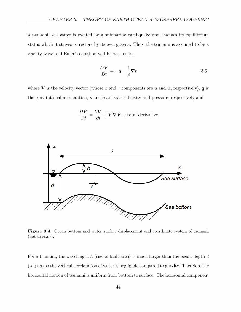
CHAPTER 3. THEORY OF EARTH-OCEAN-ATMOSPHERE COUPLING
a tsunami, sea water is excited by a submarine earthquake and changes its equilibrium
status which it strives to restore by its own gravity. Thus, the tsunami is assumed to be a
gravity wave and Euler’s equation will be written as:
DV
Dt= −g − 1
ρ∇p (3.6)
where V is the velocity vector (whose x and z components are u and w, respectively), g is
the gravitational acceleration, ρ and p are water density and pressure, respectively and
DV
Dt= ∂V
∂t+ V ∇V , a total derivative
Figure 3.4: Ocean bottom and water surface displacement and coordinate system of tsunami(not to scale).
For a tsunami, the wavelength λ (size of fault area) is much larger than the ocean depth d
(λ� d) so the vertical acceleration of water is negligible compared to gravity. Therefore the
horizontal motion of tsunami is uniform from bottom to surface. The horizontal component
44
3.3. THEORETICAL ANALYSIS OF TSUNAMI GENERATION
(on x axis) of equation 3.6 becomes:
DV
Dt= ∂u
∂t+ u
∂u
∂x≈ ∂u
∂t,
Because the nonlinear advective term is usually small for tsunami and can be therefore
ignored. Thus the equation of motion can be written as:
∂u
∂t= −g∂h
∂x(3.7)
In the deep ocean the amplitude of the tsunami is small compared to the water depth (h
� d ). The conservation of mass becomes:
∂h
∂t= −∂(du)
∂x(3.8)
From equations 3.7 and 3.8 and considering that water depth is constant, the wave equation
is given by:
∂2h
∂t2= c2∂
2h
∂x2 where c =√gd (3.9)
The velocity is then determined only by the water depth.
3.3.2 Theory of tsunami generation
Analytically, the free surface elevation h of a tsunami can be represented as a gravity wave
which one wave component is given by h (function of horizontal position x and time t):
h = a cos(kx− wt) (3.10)
45
CHAPTER 3. THEORY OF EARTH-OCEAN-ATMOSPHERE COUPLING
where a is amplitude, k wave number and ω is angular frequency.
Considering a water depth d, the phase velocity is given by the following equation:
c = ω
k=(g
ktanh(kd)
)1/2=(gλ
2π tanh(
2πdλ
))1/2
(3.11)
as discussed before, in the case of tsunami, the water depth is much smaller than the
wavelength (d � λ). Therefore, we can approximate tanh(2πd/λ) ≈ 2πd/λ, sinh(2πd/λ)
≈ 2πd/λ, cosh(k(z+d)) ≈ cosh(kd) ≈ 1. Then 3.11 goes to 3.9.
At an arbitrary height z (the seabed is at z = −d) the horizontal and vertical particle
velocities can be written as follows:
u = aω
cosh(k(z + d))sinh(kd) cos(kx− ωt)
w = aωsinh(k(z + d))
sinh(kd) sin(kx− ωt)
(3.12)
(3.13)
under the same assumption mentioned previously, the velocity ratio of equation (3.12) to
equation (3.13) is
| w | / | u |= 2πd/λ (3.14)
This quantity is very small ( dλ� 1) and indicates that for the case of tsunami, the particle
moves almost horizontally.
To get the analytical solutions of the gravity waves generated by any type of sources,
Kajiura (1963) investigated the tsunami problem and introduced the Green′s functions
for calculating sea-floor displacement (ξ) and the Green′s functions for calculating wave
elevation at the sea surface (η). He showed that the initial condition given at the ocean
46
3.4. THE RESPONSE OF SEISMOMETER TO TILT
bottom and at the water surface differ by factor of 1/cosh(kd) (equation 3.15).
η = ξ ∗(
1cosh(kd)
)= ξ ∗
(1
cosh(2πd/λ)
)(3.15)
Equation 3.15 shows that when the wavelength λ ∼ 2d then cosh(kd) ≈ exp(kd) and con-
sequently η� ξ. However, when λ� d then cosh ≈ 1. Therefore, it is theoretically proven
that the sea surface just mirrors the bottom deformation if the wavelength (horizontal size
of the tsunami at source) of ocean bottom deformation is much larger than the water depth.
Kajiura (1970) examined the energy exchange between the solid earth and ocean water
for tsunami generated by bottom deformation with finite rise time. He showed that the
efficiency of tsunami generation, defined as a ratio of dynamic tsunami energy to static
energy, becomes nearly unity if the duration is short compared to time required for tsunami
to travel through the source area.
3.4 The response of seismometer to tilt
It has been known that horizontal seismometers are sensitive not only to translation motion
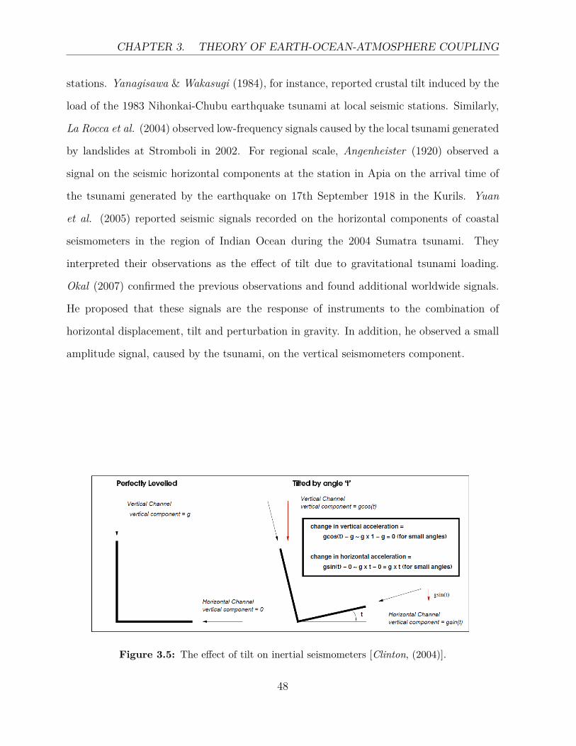
but also to tilt [Simon et al. 1967; Gladwin et al. 1987]. This is because a tilt motion
generates a gravitational force which is equivalent to an inertial force due to a translational
acceleration of the ground [Rodgers 1968]. On a very long period domain, broadband
seismometer responds positively not only to the horizontal tilt motion but to the vertical
translation motion as well but the second one has a very weak effect [Hidayat et al. 2000 ].
Traveling toward the coast, tsunamis move huge amounts of the water column with an
homogeneous velocity from bottom to the surface. This wave induces signals recorded on
seismometers and many scientists have observed its impact at local station and far field
47
CHAPTER 3. THEORY OF EARTH-OCEAN-ATMOSPHERE COUPLING
stations. Yanagisawa & Wakasugi (1984), for instance, reported crustal tilt induced by the
load of the 1983 Nihonkai-Chubu earthquake tsunami at local seismic stations. Similarly,
La Rocca et al. (2004) observed low-frequency signals caused by the local tsunami generated
by landslides at Stromboli in 2002. For regional scale, Angenheister (1920) observed a
signal on the seismic horizontal components at the station in Apia on the arrival time of
the tsunami generated by the earthquake on 17th September 1918 in the Kurils. Yuan
et al. (2005) reported seismic signals recorded on the horizontal components of coastal
seismometers in the region of Indian Ocean during the 2004 Sumatra tsunami. They
interpreted their observations as the effect of tilt due to gravitational tsunami loading.
Okal (2007) confirmed the previous observations and found additional worldwide signals.
He proposed that these signals are the response of instruments to the combination of
horizontal displacement, tilt and perturbation in gravity. In addition, he observed a small
amplitude signal, caused by the tsunami, on the vertical seismometers component.
Figure 3.5: The effect of tilt on inertial seismometers [Clinton, (2004)].
48
Chapter 4
OBSERVATION OF TSUNAMIS
4.1 Seismic observation of tsunamis
4.1.1 Introduction
Tsunami are long period gravity waves in the sea caused by vertical displacements of large
quantities of seawater. It is characterized by propagation through the whole water column
and its velocity is uniformly distributed from bottom to sea surface which allow the wave
to propagate to a very long distance. The speed of the tsunami depends on the ocean
depth. When the tsunami travels toward a shallow water the wave speed decreases but
the amplitude he wave grows up. Therefore the gravity loading of the wave propagating
toward the shore induces seismic signal on the horizontal component of the seismometer.
One of the mechanisms which may cause this signal is because the horizontal component
of seismometers is very sensitive to tilt [Gilbert 1980]. The previous chapter explained the
theory of coupling between ocean and continent as well as the response of the seismometer
to tilt effect.
49
CHAPTER 4. OBSERVATION OF TSUNAMIS
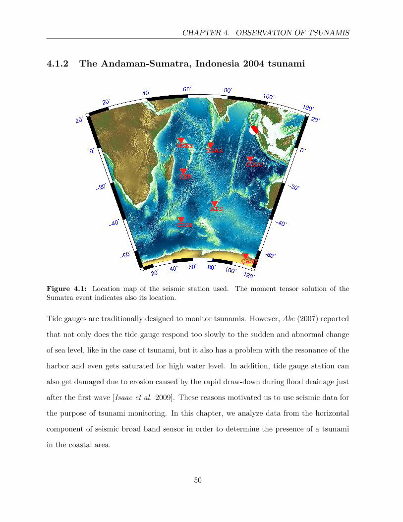
4.1.2 The Andaman-Sumatra, Indonesia 2004 tsunami
Figure 4.1: Location map of the seismic station used. The moment tensor solution of theSumatra event indicates also its location.
Tide gauges are traditionally designed to monitor tsunamis. However, Abe (2007) reported
that not only does the tide gauge respond too slowly to the sudden and abnormal change
of sea level, like in the case of tsunami, but it also has a problem with the resonance of the
harbor and even gets saturated for high water level. In addition, tide gauge station can
also get damaged due to erosion caused by the rapid draw-down during flood drainage just
after the first wave [Isaac et al. 2009]. These reasons motivated us to use seismic data for
the purpose of tsunami monitoring. In this chapter, we analyze data from the horizontal
component of seismic broad band sensor in order to determine the presence of a tsunami
in the coastal area.
50
4.1. SEISMIC OBSERVATION OF TSUNAMIS
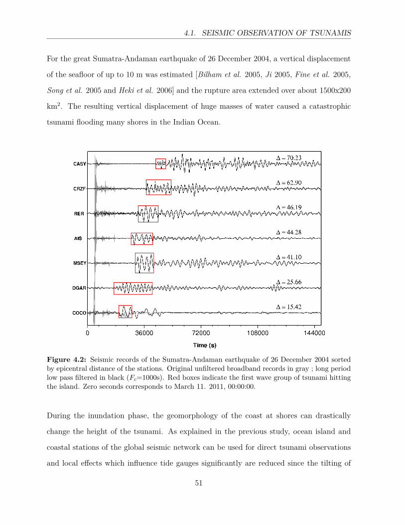
For the great Sumatra-Andaman earthquake of 26 December 2004, a vertical displacement
of the seafloor of up to 10 m was estimated [Bilham et al. 2005, Ji 2005, Fine et al. 2005,
Song et al. 2005 and Heki et al. 2006] and the rupture area extended over about 1500x200
km2. The resulting vertical displacement of huge masses of water caused a catastrophic
tsunami flooding many shores in the Indian Ocean.
Figure 4.2: Seismic records of the Sumatra-Andaman earthquake of 26 December 2004 sortedby epicentral distance of the stations. Original unfiltered broadband records in gray ; long periodlow pass filtered in black (Fc=1000s). Red boxes indicate the first wave group of tsunami hittingthe island. Zero seconds corresponds to March 11. 2011, 00:00:00.
During the inundation phase, the geomorphology of the coast at shores can drastically
change the height of the tsunami. As explained in the previous study, ocean island and
coastal stations of the global seismic network can be used for direct tsunami observations
and local effects which influence tide gauges significantly are reduced since the tilting of
51
CHAPTER 4. OBSERVATION OF TSUNAMIS
the island is an integral effect of a larger region. Yuan et al. (2005), Hanson and Bowman
(2005) and Okal (2007) observed clear effects of the Sumatra-Andaman tsunami in seismic
data. For this study, we analyze seven seismic stations in the Indian ocean [Figure 4.1] for
the determination of the arrival time of tsunami.
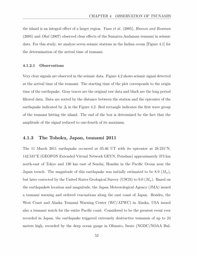
4.1.2.1 Observations
Very clear signals are observed in the seismic data. Figure 4.2 shows seismic signal detected
at the arrival time of the tsunami. The starting time of the plot corresponds to the origin
time of the earthquake. Gray traces are the original raw data and black are the long period
filtered data. Data are sorted by the distance between the station and the epicenter of the
earthquake indicated by ∆ in the Figure 4.2. Red rectangle indicates the first wave group
of the tsunami hitting the island. The end of the box is determined by the fact that the
amplitude of the signal reduced to one-fourth of its maximun.
4.1.3 The Tohoku, Japan, tsunami 2011
The 11 March 2011 earthquake occurred at 05:46 UT with its epicenter at 28.231◦N,
142.531◦E (GEOFON Extended Virtual Network GEVN, Potsdam) approximately 373 km
north-east of Tokyo and 130 km east of Sendai, Honshu in the Pacific Ocean near the
Japan trench. The magnitude of this earthquake was initially estimated to be 8.9 (Mw),
but later corrected by the United States Geological Survey (USGS) to 9.0 (Mw). Based on
the earthquake′s location and magnitude, the Japan Meteorological Agency (JMA) issued
a tsunami warning and ordered evacuations along the east coast of Japan. Besides, the
West Coast and Alaska Tsunami Warning Center (WC/ATWC) in Alaska, USA issued
also a tsunami watch for the entire Pacific coast. Considered to be the greatest event ever
recorded in Japan, the earthquake triggered extremely destructive tsunamis of up to 24
meters high, recorded by the deep ocean gauge in Ofunato, Iwate (NGDC/NOAA Bul-
52
4.1. SEISMIC OBSERVATION OF TSUNAMIS
letin), traveling several kilometers inland. The tsunami generated by this earthquake was
recorded by DART buoys and tide gauges in the Pacific Ocean.
In our observation, we infer signals detected on seismic stations caused by the average force
applied on the whole island since the entire water column is moving during the propagation
of the tsunami. Therefore, using this technique we can rule out the local effects of the beach
and can obtain the true momentum of the tsunami wave. Further analysis of the available
tide gauge data in the surrounding area close to the seismic station also allowed us to
better understand the physical mechanism of the wave and its interaction with the land.
4.1.3.1 Data
Seismic data
Seismic data recorded by broadband stations in the Pacific region were used in this study.
These stations belong to the Global Seismographic Network (GSN) and data are provided
by the Incorporated Research Institutions for Seismology (IRIS). The location of stations
is shown in Figure 4.3 represented by triangles. We requested the available seismic data in
the Pacific Ocean from the GSN/IRIS. Further examination of the data quality allows us
to select 26 permanent seismic stations located on an island or on the continental shores.
All stations analyzed in this study are listed in Table 4.1 with information about their
respective distance from shores, arrival time of the tsunami detected at seismic station and
its amplitude or ground velocity.
Tide gauge data
Tide gauge stations used in this study belong to the Center for Operational Oceanographic
Products and Services (CO-OPS). Figure 4.3 shows the location of tide gauges station used
53
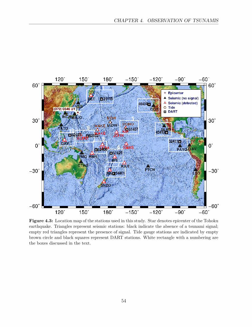
CHAPTER 4. OBSERVATION OF TSUNAMIS
Figure 4.3: Location map of the stations used in this study. Star denotes epicenter of the Tohokuearthquake. Triangles represent seismic stations: black indicate the absence of a tsunami signal;empty red triangles represent the presence of signal. Tide gauge stations are indicated by emptybrown circle and black squares represent DART stations. White rectangle with a numbering arethe boxes discussed in the text.
54
4.1. SEISMIC OBSERVATION OF TSUNAMIS
in this study (brown circle). We selected three tide gauge stations collocated in the same
Island with seismic station. However, only two of them are used here for comparison be-
cause at MIDW the seismometer had a problem few minutes after the earthquake. This
does not allow us to analyze data from MIDW in the period when tsunami is expected to
hit the island.
DART gauge data
In order to extend our observation, we look at the data from closest Deep-ocean Assessment
and Reporting of Tsunami (DATA) to the seismic station. The area where both stations
are available close to each other is marked by white rectangle on the figure 4.3. Therefore,
we used data provided by the National Oceanic and Atmospheric Administrative (NOAA).
Raw data are used from March, 11 2011.
4.1.3.2 General descriptions and observations
Surrounded by a seismically active zone along the subduction system called ”Ring of Fire”,
the Pacific basin is an home to an average number of two destructive tsunami per year [see
http://www.tulane.edu/ sanelson/geol204/tsunami.htm]. About 80 percent of the world-
wide tsunami occurs in the Pacific [Kong 2004] and one of the most vulnerable countries is
Japan. The Tohoku-Oki earthquake occurred at the Japan trench on the interface of the
Pacific and North American plates.
The Pacific plate moves approximately westwards with respect to the North America plate
at a rate of 83 mm/yr (USGS), and begins its westward descent beneath Japan at the
Japan Trench. The earthquake was caused by an abrupt release of stress which pushes
the North American plate upward and this mechanism generated the devastating tsunami.
55
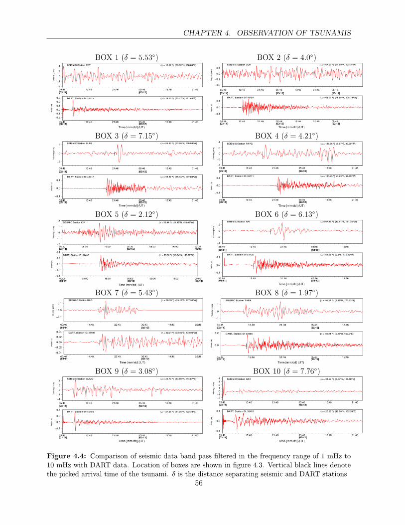
CHAPTER 4. OBSERVATION OF TSUNAMIS
BOX 1 (δ = 5.53◦) BOX 2 (δ = 4.0◦)
BOX 3 (δ = 7.15◦) BOX 4 (δ = 4.21◦)
BOX 5 (δ = 2.12◦) BOX 6 (δ = 6.13◦)
BOX 7 (δ = 5.43◦) BOX 8 (δ = 1.97◦)
BOX 9 (δ = 3.08◦) BOX 10 (δ = 7.76◦)
Figure 4.4: Comparison of seismic data band pass filtered in the frequency range of 1 mHz to10 mHz with DART data. Location of boxes are shown in figure 4.3. Vertical black lines denotethe picked arrival time of the tsunami. δ is the distance separating seismic and DART stations
56
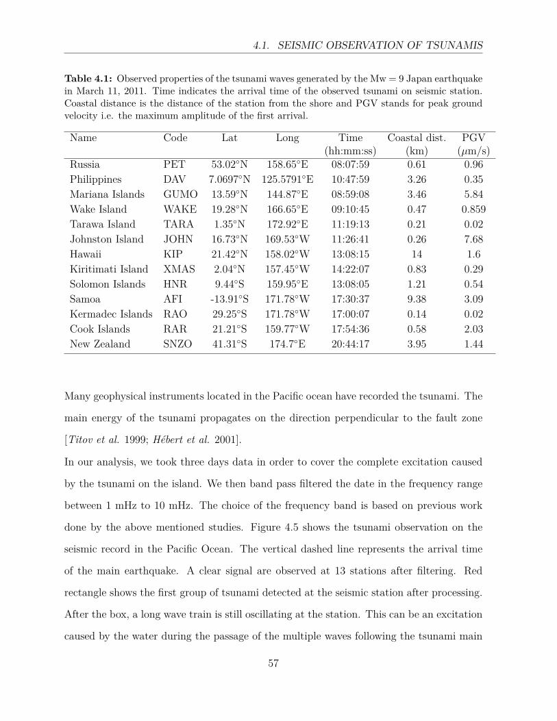
4.1. SEISMIC OBSERVATION OF TSUNAMIS
Table 4.1: Observed properties of the tsunami waves generated by the Mw = 9 Japan earthquakein March 11, 2011. Time indicates the arrival time of the observed tsunami on seismic station.Coastal distance is the distance of the station from the shore and PGV stands for peak groundvelocity i.e. the maximum amplitude of the first arrival.
Name Code Lat Long Time Coastal dist. PGV(hh:mm:ss) (km) (µm/s)
Russia PET 53.02◦N 158.65◦E 08:07:59 0.61 0.96Philippines DAV 7.0697◦N 125.5791◦E 10:47:59 3.26 0.35Mariana Islands GUMO 13.59◦N 144.87◦E 08:59:08 3.46 5.84Wake Island WAKE 19.28◦N 166.65◦E 09:10:45 0.47 0.859Tarawa Island TARA 1.35◦N 172.92◦E 11:19:13 0.21 0.02Johnston Island JOHN 16.73◦N 169.53◦W 11:26:41 0.26 7.68Hawaii KIP 21.42◦N 158.02◦W 13:08:15 14 1.6Kiritimati Island XMAS 2.04◦N 157.45◦W 14:22:07 0.83 0.29Solomon Islands HNR 9.44◦S 159.95◦E 13:08:05 1.21 0.54Samoa AFI -13.91◦S 171.78◦W 17:30:37 9.38 3.09Kermadec Islands RAO 29.25◦S 171.78◦W 17:00:07 0.14 0.02Cook Islands RAR 21.21◦S 159.77◦W 17:54:36 0.58 2.03New Zealand SNZO 41.31◦S 174.7◦E 20:44:17 3.95 1.44
Many geophysical instruments located in the Pacific ocean have recorded the tsunami. The
main energy of the tsunami propagates on the direction perpendicular to the fault zone
[Titov et al. 1999; Hébert et al. 2001].
In our analysis, we took three days data in order to cover the complete excitation caused
by the tsunami on the island. We then band pass filtered the date in the frequency range
between 1 mHz to 10 mHz. The choice of the frequency band is based on previous work
done by the above mentioned studies. Figure 4.5 shows the tsunami observation on the
seismic record in the Pacific Ocean. The vertical dashed line represents the arrival time
of the main earthquake. A clear signal are observed at 13 stations after filtering. Red
rectangle shows the first group of tsunami detected at the seismic station after processing.
After the box, a long wave train is still oscillating at the station. This can be an excitation
caused by the water during the passage of the multiple waves following the tsunami main
57
CHAPTER 4. OBSERVATION OF TSUNAMIS
energy plus the reflected waves from the surrounding coastal area. The signal can last for
about one hour (Kiritimati Island, XMAS) but might oscillate for several hours and even
days (New Zealand, SNZO). Tsunami signal are mainly observed on the same direction
as the main lobe of potential energy dissipated by the tsunami. Note that the maximum
energy of the tsunami generated by an earthquake on a fault zone is always perpendicular
to the direction of the fault.
Figure 4.4 shows the comparison between low pass filtered seismic data and raw data ob-
tained from the closest DART station. The distance δ between two stations varies from
1.97◦ (BOX 8) to 7.76◦ (BOX 10). In general, the observed signal on the seismic station
corresponds to the arrival time of the tsunami on the DART station despite the difference
in terms of frequency content between two data. This confirms that seismic station can be
used as tsunameter even at some distance away from the shore line.
In box 2 we did not observed any signal on the seismic record because the SNR is very
weak. In box 3 late arrival of the signal is observed on the seismic trace though seismic
station is located closer to the source than the DART station. This might be a signal
caused by waves which get trapped in the gulf of California after the passage of the head-
ing tsunami and have grown-up and inundated the area. However, seismic signal on box 4
arrives earlier than the tsunami recorded on the DART station despite seismic station is
farther from source than DART station. The signal observed on the seismic station can be
caused by different source other than tsunami. In box 6, the late arrival of the signal is due
to the ocean depth. Actually the tsunami travels at a speed of 50 m/s which correspond
to shallow water similarly to the case here. At the seismic station DAV in box 10, a very
weak signal is observed which travels as slow as the tsunami in box 6.
58
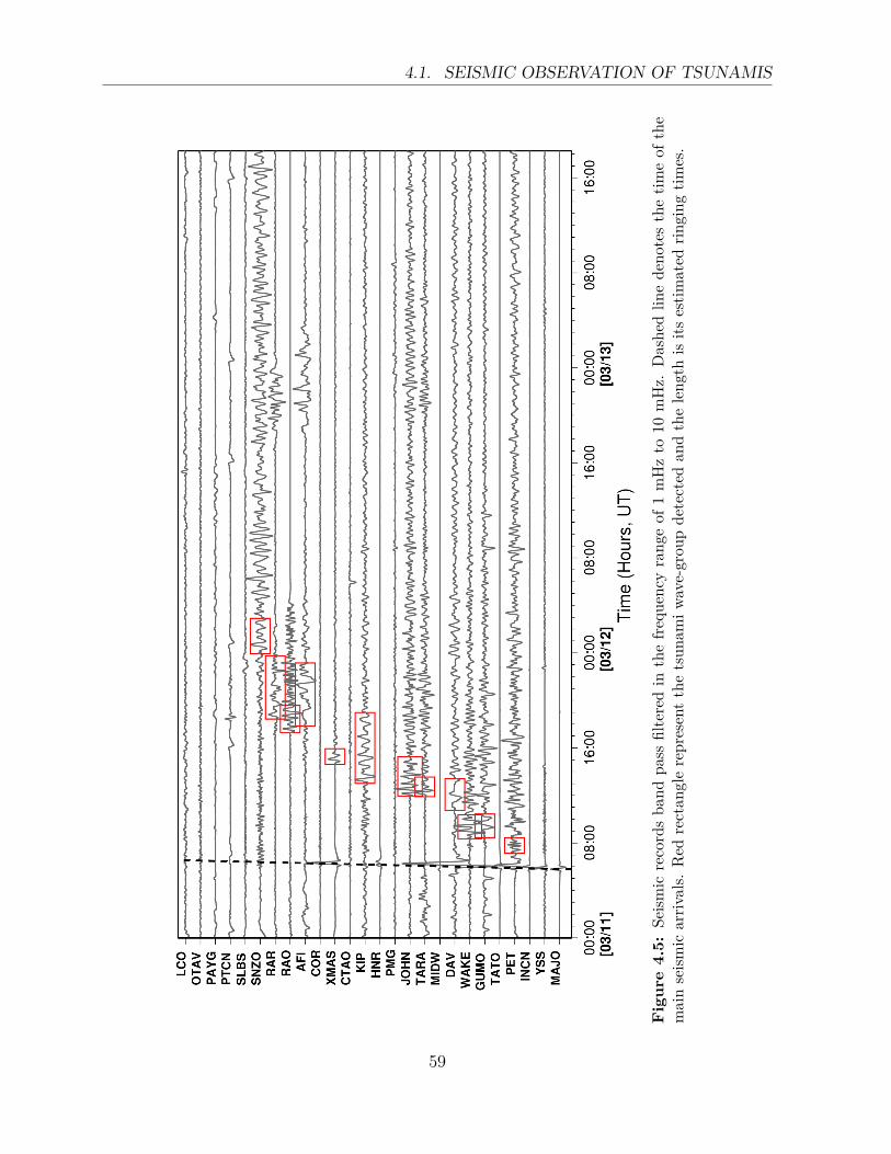
4.1. SEISMIC OBSERVATION OF TSUNAMIS
Fig
ure
4.5:
Seism
icre
cord
sba
ndpa
ssfil
tere
din
the
freq
uenc
yra
nge
of1
mH
zto
10m
Hz.
Das
hed
line
deno
tes
the
time
ofth
em
ain
seism
icar
rival
s.R
edre
ctan
gle
repr
esen
tth
ets
unam
iwav
e-gr
oup
dete
cted
and
the
leng
this
itses
timat
edrin
ging
times
.
59
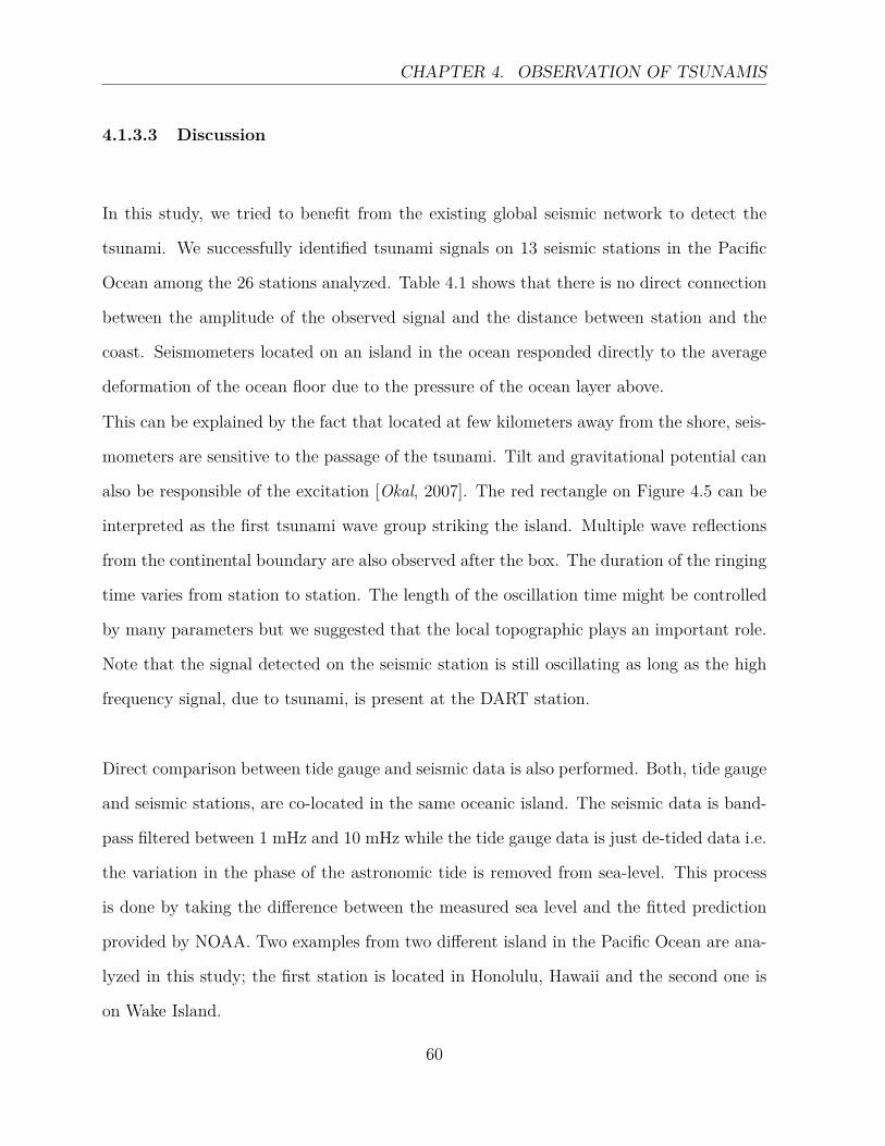
CHAPTER 4. OBSERVATION OF TSUNAMIS
4.1.3.3 Discussion
In this study, we tried to benefit from the existing global seismic network to detect the
tsunami. We successfully identified tsunami signals on 13 seismic stations in the Pacific
Ocean among the 26 stations analyzed. Table 4.1 shows that there is no direct connection
between the amplitude of the observed signal and the distance between station and the
coast. Seismometers located on an island in the ocean responded directly to the average
deformation of the ocean floor due to the pressure of the ocean layer above.
This can be explained by the fact that located at few kilometers away from the shore, seis-
mometers are sensitive to the passage of the tsunami. Tilt and gravitational potential can
also be responsible of the excitation [Okal, 2007]. The red rectangle on Figure 4.5 can be
interpreted as the first tsunami wave group striking the island. Multiple wave reflections
from the continental boundary are also observed after the box. The duration of the ringing
time varies from station to station. The length of the oscillation time might be controlled
by many parameters but we suggested that the local topographic plays an important role.
Note that the signal detected on the seismic station is still oscillating as long as the high
frequency signal, due to tsunami, is present at the DART station.
Direct comparison between tide gauge and seismic data is also performed. Both, tide gauge
and seismic stations, are co-located in the same oceanic island. The seismic data is band-
pass filtered between 1 mHz and 10 mHz while the tide gauge data is just de-tided data i.e.
the variation in the phase of the astronomic tide is removed from sea-level. This process
is done by taking the difference between the measured sea level and the fitted prediction
provided by NOAA. Two examples from two different island in the Pacific Ocean are ana-
lyzed in this study; the first station is located in Honolulu, Hawaii and the second one is
on Wake Island.
60
4.1. SEISMIC OBSERVATION OF TSUNAMIS
Figure 4.6: Comparison of seismic and tide gauge and DART data in Hawaii. Top: Map showingthe location of seismic, tide gauge and DART stations. Bottom:(a) Seismic data bandpass filteredbetween 1mHz and 10 mHz.(b) de-tided tide gauge data.(c) DART data
61
CHAPTER 4. OBSERVATION OF TSUNAMIS
On the first example of the Hawaii station in Figure 4.6 we noticed a perfect agreement
between the two waveforms for about 10 hours from the moment when tsunami hits the
Island. Despite the remarkable background oscillations, caused by the earthquake, before
of the signal (red trace from 06:00 to 13:00) the SNR remains very good which allow us to
see a very clear signal. Located at about 20 km away from the tide gauge station, a good
correlation is observed between the seismic and the tide gauge signal. Note that the seismic
signal arrived relatively earlier than the actual arrival time of the tsunami . However, the
duration of ringing observed at both stations as well as the amplitude decay is relatively
similar.
DART station located at about 200 km away from the two previous stations is also an-
alyzed. It is confirmed that the signal observed on the seismic station is exactly caused
by the excitation of tsunami. The late arrival is due to the distance and the water depth.
For the second example, same procedure is used for the comparison of seismic and tide
gauge data in Wake Island (Figure 4.7). Similarly to the previous example, the tsunami is
observed on both records. However, one of the very remarkable observation is the polarity
of the leading wave on both traces. If the seismic signal observed a negative leading wave,
we note a positive amplitude on the first arrival on the tide gauge data. This should be
an effect of the geometry of the island with respect to the location of the two stations.
Wake island is ”V”-shaped pointed towards the southeast surrounded by deep water and
inside the two legs of the ”V” is a lagoon. The seismic station (WAKE) is located at the
east coast of the Island whereas the tide gauge is inside the two legs of the ”V” (Figure
4.7). We noticed also the presence of high frequency signal on the tide gauge data. This
is interpreted as the resonance of the tsunami wave trains in the channel between the two
legs of that ”V”; the tsunami came inside the two legs and gets trapped there. These high
frequency wave trains are not observed in the seismic data (red trace). The energy decay
62
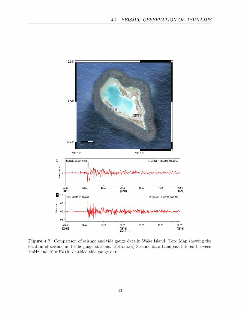
4.1. SEISMIC OBSERVATION OF TSUNAMIS
Figure 4.7: Comparison of seismic and tide gauge data in Wake Island. Top: Map showing thelocation of seismic and tide gauge stations. Bottom:(a) Seismic data bandpass filtered between1mHz and 10 mHz.(b) de-tided tide gauge data.
63
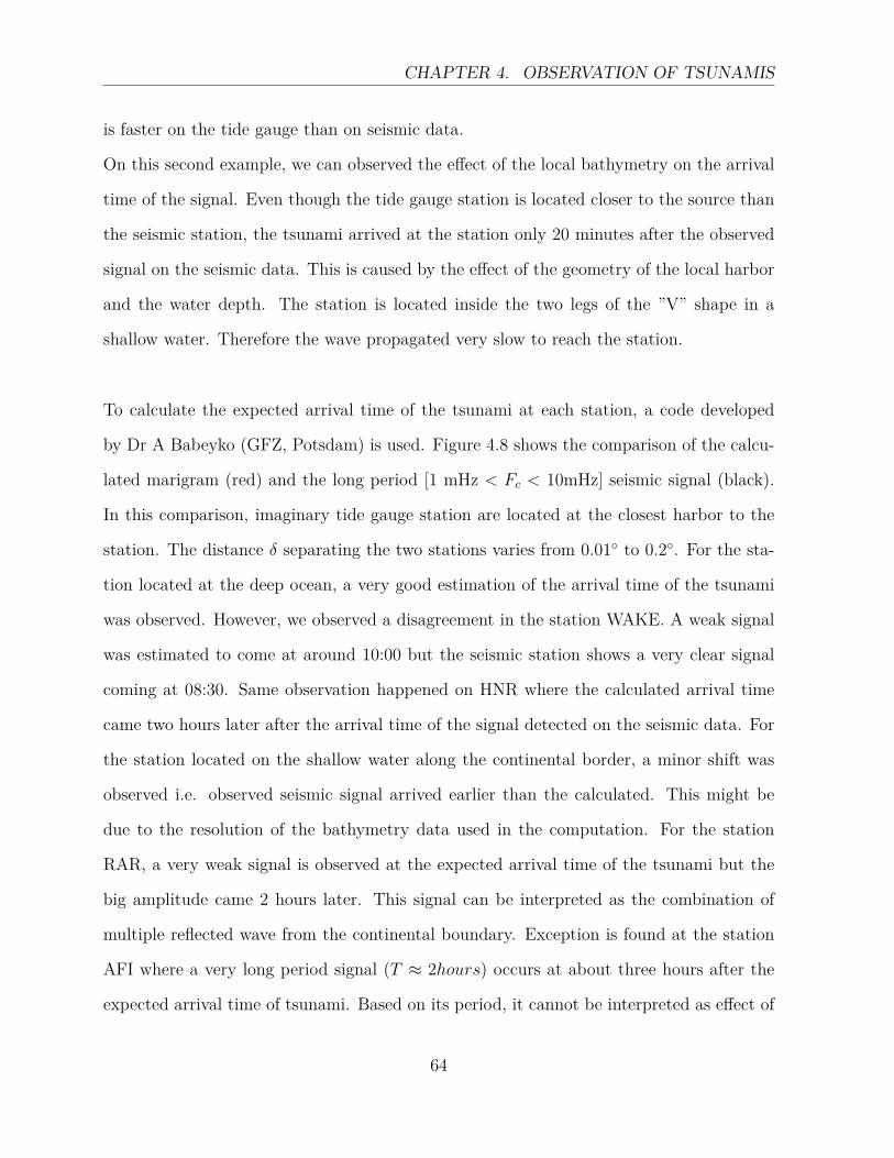
CHAPTER 4. OBSERVATION OF TSUNAMIS
is faster on the tide gauge than on seismic data.
On this second example, we can observed the effect of the local bathymetry on the arrival
time of the signal. Even though the tide gauge station is located closer to the source than
the seismic station, the tsunami arrived at the station only 20 minutes after the observed
signal on the seismic data. This is caused by the effect of the geometry of the local harbor
and the water depth. The station is located inside the two legs of the ”V” shape in a
shallow water. Therefore the wave propagated very slow to reach the station.
To calculate the expected arrival time of the tsunami at each station, a code developed
by Dr A Babeyko (GFZ, Potsdam) is used. Figure 4.8 shows the comparison of the calcu-
lated marigram (red) and the long period [1 mHz < Fc < 10mHz] seismic signal (black).
In this comparison, imaginary tide gauge station are located at the closest harbor to the
station. The distance δ separating the two stations varies from 0.01◦ to 0.2◦. For the sta-
tion located at the deep ocean, a very good estimation of the arrival time of the tsunami
was observed. However, we observed a disagreement in the station WAKE. A weak signal
was estimated to come at around 10:00 but the seismic station shows a very clear signal
coming at 08:30. Same observation happened on HNR where the calculated arrival time
came two hours later after the arrival time of the signal detected on the seismic data. For
the station located on the shallow water along the continental border, a minor shift was
observed i.e. observed seismic signal arrived earlier than the calculated. This might be
due to the resolution of the bathymetry data used in the computation. For the station
RAR, a very weak signal is observed at the expected arrival time of the tsunami but the
big amplitude came 2 hours later. This signal can be interpreted as the combination of
multiple reflected wave from the continental boundary. Exception is found at the station
AFI where a very long period signal (T ≈ 2hours) occurs at about three hours after the
expected arrival time of tsunami. Based on its period, it cannot be interpreted as effect of
64
4.1. SEISMIC OBSERVATION OF TSUNAMIS
Figure 4.8: Seismic records (black) band pass filtered [1 to 10 mHz] and calculated marigram(red) located offshore. δ represents the distance between seismic station and the imaginary tidegauge station
65
CHAPTER 4. OBSERVATION OF TSUNAMIS
tsunami.
4.1.3.4 Conclusion
We have shown that for oceanic islands the distance of the seismic station from the shore
does not affect much the amplitude of the ground velocity recorded caused by a tsunami.
By doing a direct comparison of tide gauge and seismic data, we conclude that the seismic
signal observed after filtering is comparable to the tsunami recorded by tide gauge because
of the similarity between the filtered seismic wave shape and the de-tided tide gauge data
as well as the good agreement with the tsunami arrival time. We suggest that broad band
seismic stations on oceanic islands have the potential to contribute significant information
for the purpose of tsunami monitoring. Expected arrival times of the tsunami, estimated
from the theoretical marigrams, confirms that tsunami did generate signal which can be
recorded by seismometer. Late arrival in some stations shows that the initial wave is
not necessarily the largest and tsunamis can be dangerous for many hours after arrival.
The signal observed at seismic stations during the tsunami is more consistent because it
represents the average response of the whole island. Additionally, seismic stations are safe
from damage due to erosion caused by the rapid draw down during flood drainage and free
from the resonance of the harbor.
4.2 Infrasound observation of tsunamis
4.2.1 Introduction
Our motivation to analyze atmospheric data is based on the theory of the coupling mech-
anism existed between the ocean and the atmosphere explained in previous chapter. Note
that there exist three main categories of sound waves in the atmosphere. The principal one
66
4.2. INFRASOUND OBSERVATION OF TSUNAMIS
is the audible sound which is a wave traveling in the atmosphere with a frequency range of
20 to 20000 Hz. The next category of waves in the frequency range beyond 20000 Hz, the
sound is known as an ultrasound and it is an inaudible sound. Animals like bats use such
very high frequency wave as sonar for orientation. The third category is sound used by
elephants for their communication over long distances by stomping their feet and sending
vibration through the ground. This category of wave oscillates at a frequency lower than
20 Hz and cannot be heard by the human ears. It is known as ”infrasound” and propagates
at a speed of sound 343 m/s at 20 ◦ C in the air near the earth’s surface. In this chapter,
our attempt is to use infrasound data to detect signal generated by a tsunami into the
atmosphere.
In the following paragraphs, the infrasound method refers to the measurement of the
atmospheric pressure changes caused by different sources which disturb the equilibrium
state of the air. Initially, the Allied forces used this technique during the World War I in
order to locate artillery. This topic was considered as a top secret topic during the cold
war period and very few people worked on infrasound data. In 1996, the general assembly
of the Comprehensive Nuclear Test Ban Treaty Organization(CTBTO) required that a
global network of infrasound station, composed of 60 stations, will be installed in order to
detect and identify possible nuclear explosions. Since a few years ago, infrasound data is
thus accessible for selected scientists. As a result, considerable progress has been made in
atmospheric monitoring based on infrasound data analysis [Brachet et al. 2010].
4.2.2 Infrasound data
The infrasound data used in this study are from the network of the International Monitor-
ing System (IMS) of the CTBTO in Vienna, Austria. Such an infrasound station consists
of four to eight elements and the distance between elements varies from 1 to 3 km. Each
67
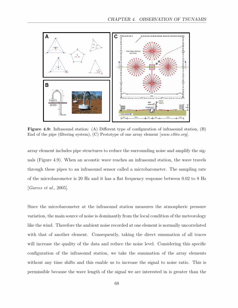
CHAPTER 4. OBSERVATION OF TSUNAMIS
Figure 4.9: Infrasound station: (A) Different type of configuration of infrasound station, (B)End of the pipe (filtering system), (C) Prototype of one array element [www.ctbto.org].
array element includes pipe structures to reduce the surrounding noise and amplify the sig-
nals (Figure 4.9). When an acoustic wave reaches an infrasound station, the wave travels
through these pipes to an infrasound sensor called a microbarometer. The sampling rate
of the microbarometer is 20 Hz and it has a flat frequency response between 0.02 to 8 Hz
[Garces et al., 2005].
Since the microbarometer at the infrasound station measures the atmospheric pressure
variation, the main source of noise is dominantly from the local condition of the meteorology
like the wind. Therefore the ambient noise recorded at one element is normally uncorrelated
with that of another element. Consequently, taking the direct summation of all traces
will increase the quality of the data and reduce the noise level. Considering this specific
configuration of the infrasound station, we take the summation of the array elements
without any time shifts and this enable us to increase the signal to noise ratio. This is
permissible because the wave length of the signal we are interested in is greater than the
68
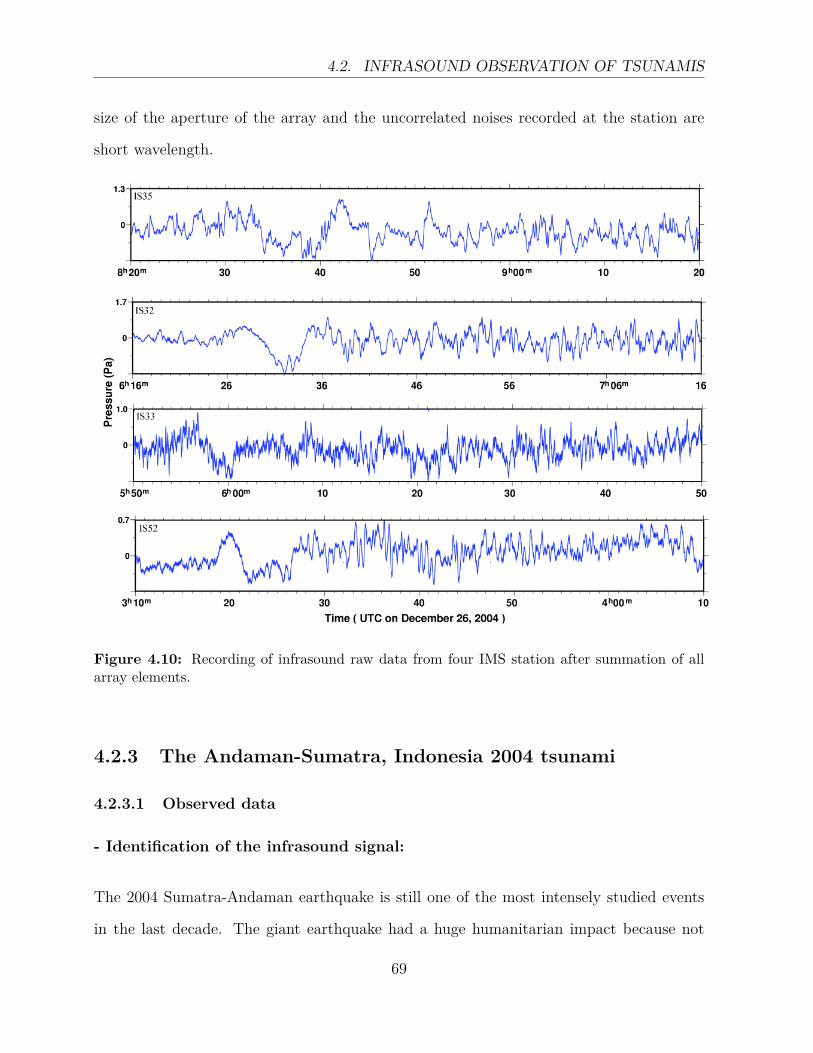
4.2. INFRASOUND OBSERVATION OF TSUNAMIS
size of the aperture of the array and the uncorrelated noises recorded at the station are
short wavelength.
Figure 4.10: Recording of infrasound raw data from four IMS station after summation of allarray elements.
4.2.3 The Andaman-Sumatra, Indonesia 2004 tsunami
4.2.3.1 Observed data
- Identification of the infrasound signal:
The 2004 Sumatra-Andaman earthquake is still one of the most intensely studied events
in the last decade. The giant earthquake had a huge humanitarian impact because not
69

CHAPTER 4. OBSERVATION OF TSUNAMIS
only did it destroy local infrastructures but it also triggered a devastating tsunami along
the coasts of most countries around the Indian Ocean which cost many lives In the realm
of science the Sumatra-Andaman event was very interesting because it was recorded by
many instruments, on the ground as high as in the ionosphere [Artru et al. 2005], even
those which are not designed for tsunami monitoring like microbarometers deployed at an
infrasound station. Therefore, four infrasound stations in the indian ocean rim detected
signal from the tsunami. The summation of all raw data from each element of the station
is presented in Figure 4.10. High frequency noises is eliminated in the first two top panels
(IS35 and IS32). However, the station IS33, in the lower middle panel, is dominated by
high frequencies which can be explained as other source of signal present in the whole
array. The length of the time window used here is 60 minutes. The time windows at
each station starts 10 min before the expected arrival time of the signal estimated from
the average speed of tsunami in the deep ocean. For the detection of the event, we used
all the data from each element of the array. In Figure 4.11, a second order Butterworth
band-pass filter has been applied to the data with corner frequency of 1.19 and 4.16 mHz.
The arrival time of signal caused by the tsunami are marked by vertical green lines which
can be easily detected by the presence of coherent signals in at least three elements of the
array. We used the elements where data is available. As an example, for the station IS35
only three elements (I35H2, I35H3, I35H4) of the array have data at the moment of the
event. We observed also clear signal with good coherence arriving around 3:00 UT at the
station IS52 prior to the arrival time of the tsunami air wave. These signals correspond
to the pressure disturbance during the passage of large amplitude surface waves under the
station circling the earth.
- Location of infrasound source:
70
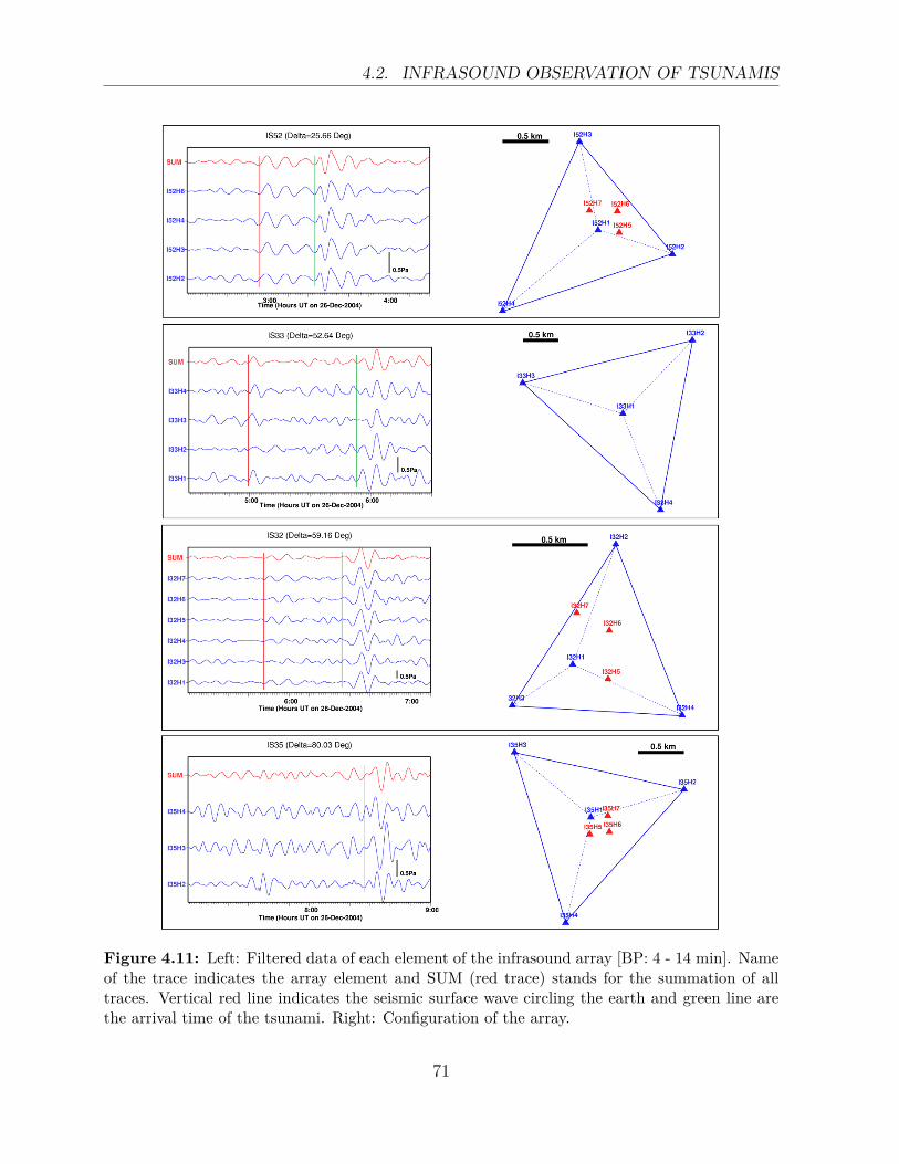
4.2. INFRASOUND OBSERVATION OF TSUNAMIS
Figure 4.11: Left: Filtered data of each element of the infrasound array [BP: 4 - 14 min]. Nameof the trace indicates the array element and SUM (red trace) stands for the summation of alltraces. Vertical red line indicates the seismic surface wave circling the earth and green line arethe arrival time of the tsunami. Right: Configuration of the array.
71
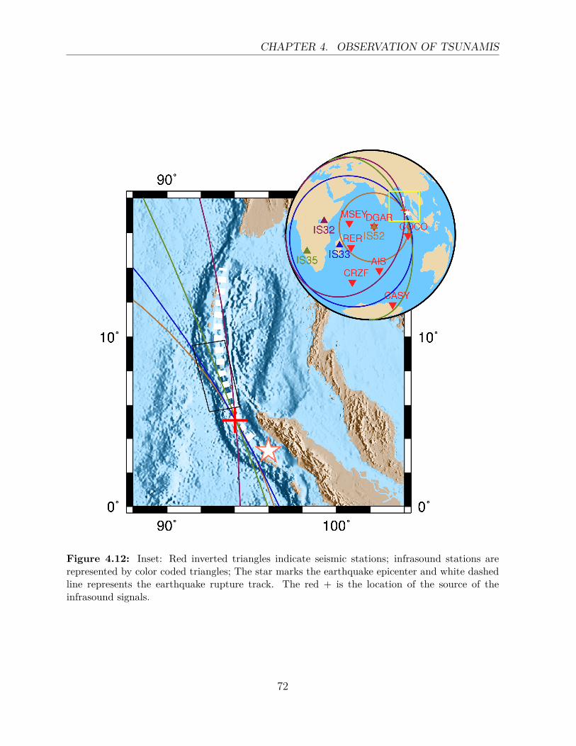
CHAPTER 4. OBSERVATION OF TSUNAMIS
Figure 4.12: Inset: Red inverted triangles indicate seismic stations; infrasound stations arerepresented by color coded triangles; The star marks the earthquake epicenter and white dashedline represents the earthquake rupture track. The red + is the location of the source of theinfrasound signals.
72
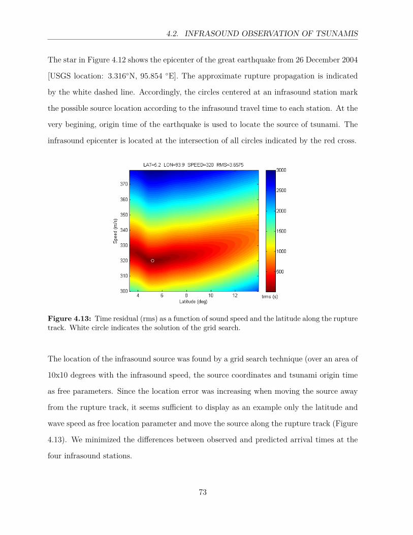
4.2. INFRASOUND OBSERVATION OF TSUNAMIS
The star in Figure 4.12 shows the epicenter of the great earthquake from 26 December 2004
[USGS location: 3.316◦N, 95.854 ◦E]. The approximate rupture propagation is indicated
by the white dashed line. Accordingly, the circles centered at an infrasound station mark
the possible source location according to the infrasound travel time to each station. At the
very begining, origin time of the earthquake is used to locate the source of tsunami. The
infrasound epicenter is located at the intersection of all circles indicated by the red cross.
Figure 4.13: Time residual (rms) as a function of sound speed and the latitude along the rupturetrack. White circle indicates the solution of the grid search.
The location of the infrasound source was found by a grid search technique (over an area of
10x10 degrees with the infrasound speed, the source coordinates and tsunami origin time
as free parameters. Since the location error was increasing when moving the source away
from the rupture track, it seems sufficient to display as an example only the latitude and
wave speed as free location parameter and move the source along the rupture track (Figure
4.13). We minimized the differences between observed and predicted arrival times at the
four infrasound stations.
73
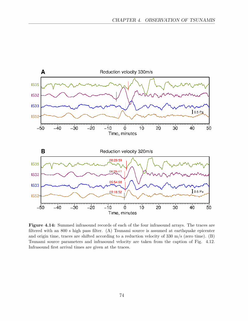
CHAPTER 4. OBSERVATION OF TSUNAMIS
Figure 4.14: Summed infrasound records of each of the four infrasound arrays. The traces arefiltered with an 800 s high pass filter. (A) Tsunami source is assumed at earthquake epicenterand origin time, traces are shifted according to a reduction velocity of 330 m/s (zero time). (B)Tsunami source parameters and infrasound velocity are taken from the caption of Fig. 4.12.Infrasound first arrival times are given at the traces.
74

4.2. INFRASOUND OBSERVATION OF TSUNAMIS
The best solution was found for an infrasound speed of 320 m/s and a source location
at 5◦N latitude and 94◦řE longitude (red cross in Figure 4.12A). A delay of 108 s of the
tsunami origin time relative to the origin time of the earthquake was obtained. This fits
well with the rupture velocity of 2.6 km/s obtained by Lay et al. (2005). Our infrasound
source is located about 200 km to the south of the location by Mikumo et al. (2008), who
derived their location from modeling of first arrival times and amplitudes of infrasound
phases (black box in Figure 4.12A) with an extended source. Our location coincide to the
maximum of co and post-seismic slip distribution on the Sunda megathrust estimated from
inversion of geodetic data [Subarya, et al. 2006]
In Figure 4.14 infrasound waveforms are displayed with time shifts according to different
source parameters. In Figure 4.14A the epicenter is assumed as source of the infrasound
signal; in Figure 4.14B the source parameters determined by the grid search are used. The
arrival times of the first infrasound signal are marked in Figure 4.14B. This figure also
shows the good signal-to-noise ratio and the great similarity of the infrasound signals at
all stations. Assuming the epicentral source and origin time of the earthquake to be the
same as the source of infrasound fails to predict the arrival time.
4.2.3.2 Synthetic data
In order to better understand the physical process of the interaction of the tsunami with
the atmosphere and continent, we analyze theoretical data. The synthetics are calculated
using code developed by Wang (1999) based on normal mode theory [Gilbert and Backus
1968, Takeuchi and Saito 1972] and the orthonormalized matrix algorithm of Wang (1999)
for numerical stability. The seismic reference model PREM is used for the computations
for the seismic response at the ocean bottom.
75

CHAPTER 4. OBSERVATION OF TSUNAMIS
Figure 4.15: US Standard Atmosphere model.(http://science.jrank.org/pages/65157/standard-atmosphere.html)
For a better fitting of the tsunami propagation velocity in the Indian Ocean, we changed
the thickness of ocean layer in the original PREM model from 3 to 4 km and added a stan-
dard atmosphere above it (US Standard Atmosphere 1976, see Figure 4.15). Tilt effects
due to gravitational tsunami loading are included in the calculation of seismic synthetics,
but no instrumental effect is included.
Figure 4.16: Example of synthetic infrasound trace of the great Sumatra-Andaman earthquake.TS indicates the arrival of tsunami air wave.(Source parameters: Harvard CMT Double-Couple solution - Earth model: PREM + US StandardAtmosphere)
76
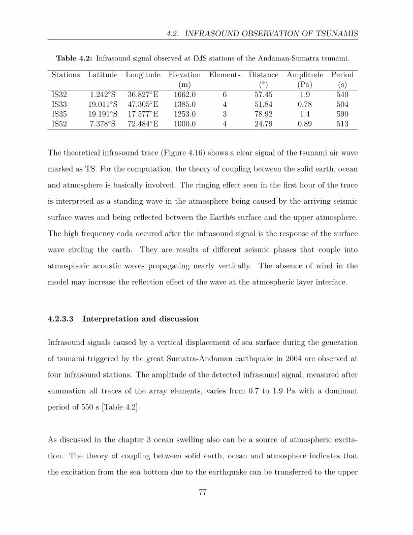
4.2. INFRASOUND OBSERVATION OF TSUNAMIS
Table 4.2: Infrasound signal observed at IMS stations of the Andaman-Sumatra tsunami.
Stations Latitude Longitude Elevation Elements Distance Amplitude Period(m) (◦) (Pa) (s)
IS32 1.242◦S 36.827◦E 1662.0 6 57.45 1.9 540IS33 19.011◦S 47.305◦E 1385.0 4 51.84 0.78 504IS35 19.191◦S 17.577◦E 1253.0 3 78.92 1.4 590IS52 7.378◦S 72.484◦E 1000.0 4 24.79 0.89 513
The theoretical infrasound trace (Figure 4.16) shows a clear signal of the tsunami air wave
marked as TS. For the computation, the theory of coupling between the solid earth, ocean
and atmosphere is basically involved. The ringing effect seen in the first hour of the trace
is interpreted as a standing wave in the atmosphere being caused by the arriving seismic
surface waves and being reflected between the Earth′s surface and the upper atmosphere.
The high frequency coda occured after the infrasound signal is the response of the surface
wave circling the earth. They are results of different seismic phases that couple into
atmospheric acoustic waves propagating nearly vertically. The absence of wind in the
model may increase the reflection effect of the wave at the atmospheric layer interface.
4.2.3.3 Interpretation and discussion
Infrasound signals caused by a vertical displacement of sea surface during the generation
of tsunami triggered by the great Sumatra-Andaman earthquake in 2004 are observed at
four infrasound stations. The amplitude of the detected infrasound signal, measured after
summation all traces of the array elements, varies from 0.7 to 1.9 Pa with a dominant
period of 550 s [Table 4.2].
As discussed in the chapter 3 ocean swelling also can be a source of atmospheric excita-
tion. The theory of coupling between solid earth, ocean and atmosphere indicates that
the excitation from the sea bottom due to the earthquake can be transferred to the upper
77
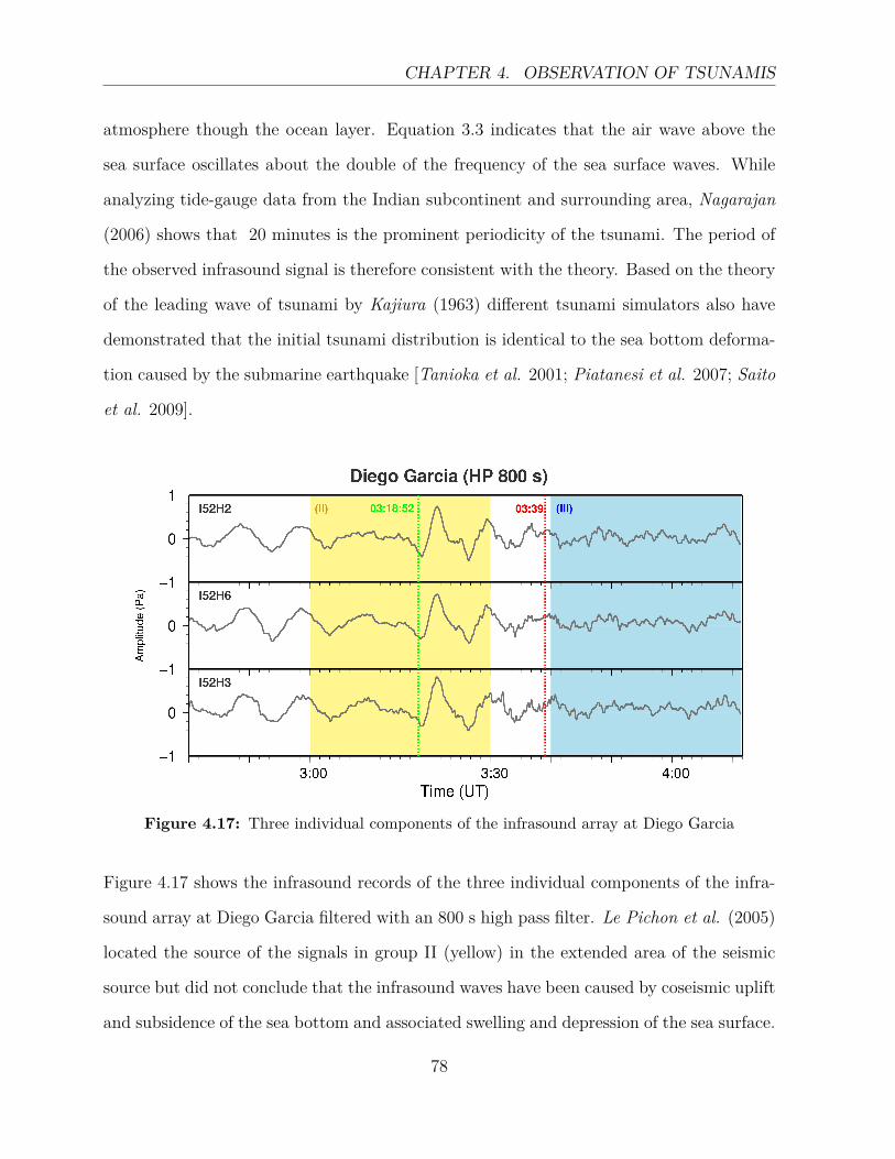
CHAPTER 4. OBSERVATION OF TSUNAMIS
atmosphere though the ocean layer. Equation 3.3 indicates that the air wave above the
sea surface oscillates about the double of the frequency of the sea surface waves. While
analyzing tide-gauge data from the Indian subcontinent and surrounding area, Nagarajan
(2006) shows that 20 minutes is the prominent periodicity of the tsunami. The period of
the observed infrasound signal is therefore consistent with the theory. Based on the theory
of the leading wave of tsunami by Kajiura (1963) different tsunami simulators also have
demonstrated that the initial tsunami distribution is identical to the sea bottom deforma-
tion caused by the submarine earthquake [Tanioka et al. 2001; Piatanesi et al. 2007; Saito
et al. 2009].
Figure 4.17: Three individual components of the infrasound array at Diego Garcia
Figure 4.17 shows the infrasound records of the three individual components of the infra-
sound array at Diego Garcia filtered with an 800 s high pass filter. Le Pichon et al. (2005)
located the source of the signals in group II (yellow) in the extended area of the seismic
source but did not conclude that the infrasound waves have been caused by coseismic uplift
and subsidence of the sea bottom and associated swelling and depression of the sea surface.
78
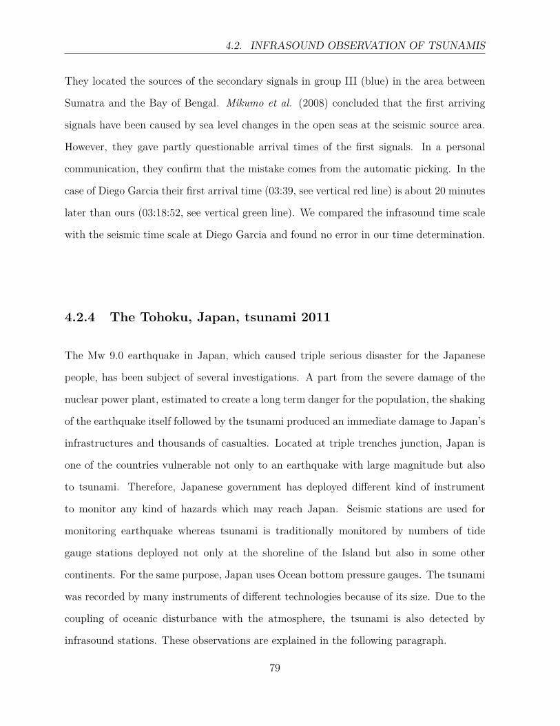
4.2. INFRASOUND OBSERVATION OF TSUNAMIS
They located the sources of the secondary signals in group III (blue) in the area between
Sumatra and the Bay of Bengal. Mikumo et al. (2008) concluded that the first arriving
signals have been caused by sea level changes in the open seas at the seismic source area.
However, they gave partly questionable arrival times of the first signals. In a personal
communication, they confirm that the mistake comes from the automatic picking. In the
case of Diego Garcia their first arrival time (03:39, see vertical red line) is about 20 minutes
later than ours (03:18:52, see vertical green line). We compared the infrasound time scale
with the seismic time scale at Diego Garcia and found no error in our time determination.
4.2.4 The Tohoku, Japan, tsunami 2011
The Mw 9.0 earthquake in Japan, which caused triple serious disaster for the Japanese
people, has been subject of several investigations. A part from the severe damage of the
nuclear power plant, estimated to create a long term danger for the population, the shaking
of the earthquake itself followed by the tsunami produced an immediate damage to Japan’s
infrastructures and thousands of casualties. Located at triple trenches junction, Japan is
one of the countries vulnerable not only to an earthquake with large magnitude but also
to tsunami. Therefore, Japanese government has deployed different kind of instrument
to monitor any kind of hazards which may reach Japan. Seismic stations are used for
monitoring earthquake whereas tsunami is traditionally monitored by numbers of tide
gauge stations deployed not only at the shoreline of the Island but also in some other
continents. For the same purpose, Japan uses Ocean bottom pressure gauges. The tsunami
was recorded by many instruments of different technologies because of its size. Due to the
coupling of oceanic disturbance with the atmosphere, the tsunami is also detected by
infrasound stations. These observations are explained in the following paragraph.
79
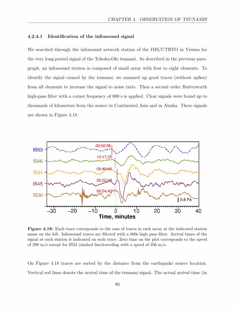
CHAPTER 4. OBSERVATION OF TSUNAMIS
4.2.4.1 Identification of the infrasound signal
We searched through the infrasound network station of the IMS/CTBTO in Vienna for
the very long-period signal of the Tohoku-Oki tsunami. As described in the previous para-
graph, an infrasound station is composed of small array with four to eight elements. To
identify the signal caused by the tsunami, we summed up good traces (without spikes)
from all elements to increase the signal to noise ratio. Then a second order Butterworth
high-pass filter with a corner frequency of 800 s is applied. Clear signals were found up to
thousands of kilometers from the source in Continental Asia and in Alaska. These signals
are shown in Figure 4.18.
Figure 4.18: Each trace corresponds to the sum of traces in each array at the indicated stationname on the left. Infrasound traces are filtered with a 800s high pass filter. Arrival times of thesignal at each station is indicated on each trace. Zero time on the plot corresponds to the speedof 290 m/s except for IS53 (dashed line)traveling with a speed of 356 m/s.
On Figure 4.18 traces are sorted by the distance from the earthquake source location.
Vertical red lines denote the arrival time of the tsunami signal. The actual arrival time (in
80
4.2. INFRASOUND OBSERVATION OF TSUNAMIS
UT) is mentioned next to these line. The period of the detected signals varies from500 s
to 800 s and the signal travels with a speed of 290 m/s for the Asian stations and 356
m/s for the station in Alaska [see table 4.3].
4.2.4.2 Location of the infrasound source
During the tsunamigenic earthquake in Tohoku-Oki, Japan the sea floor is displaced ver-
tically. These displacements are shown in Figure 4.19 -A by red arrows computed by
using GPS/acoustic combination techniques. These values are the difference between the
sea floor depth observed before (2010) and after (2011)the event [Sato, et al., 2011]. As
explained in the previous chapter, the energy released during that vertical displacement
is transferred into the ocean which in turn produces a vertical displacement on the sea
surface above the hypocenter of the earthquake. The sudden vertical displacement of the
sea surface generates an acoustic gravity wave in the atmosphere which was detectable by
infrasound stations. We used these detected signals to locate the source of the tsunami.
The location of the tsunami source is done by a grid search over the coordinates of the
tsunami source location and the sound speed. The search is done within area of 4X4degrees
around the epicenter of the earthquake. By knowing the arrival time of the signal, we
choose one arbitrary speed and consider it as zero time. Then we align all the signal to
the zero line by doing reduction speed and we keep on changing the speed until we find
a location where the time difference between the zero line and the arrival time is very small.
The origin time of the earthquake was used as the tsunami origin time. Figure 4.20 shows
the large view of the whole station. Here, similar technique formally used in seismology
for locating earthquake is used. In each station, we draw a circle centered at the station
itself and the radius of the circle is equal to the product of the propagation speed and the
81
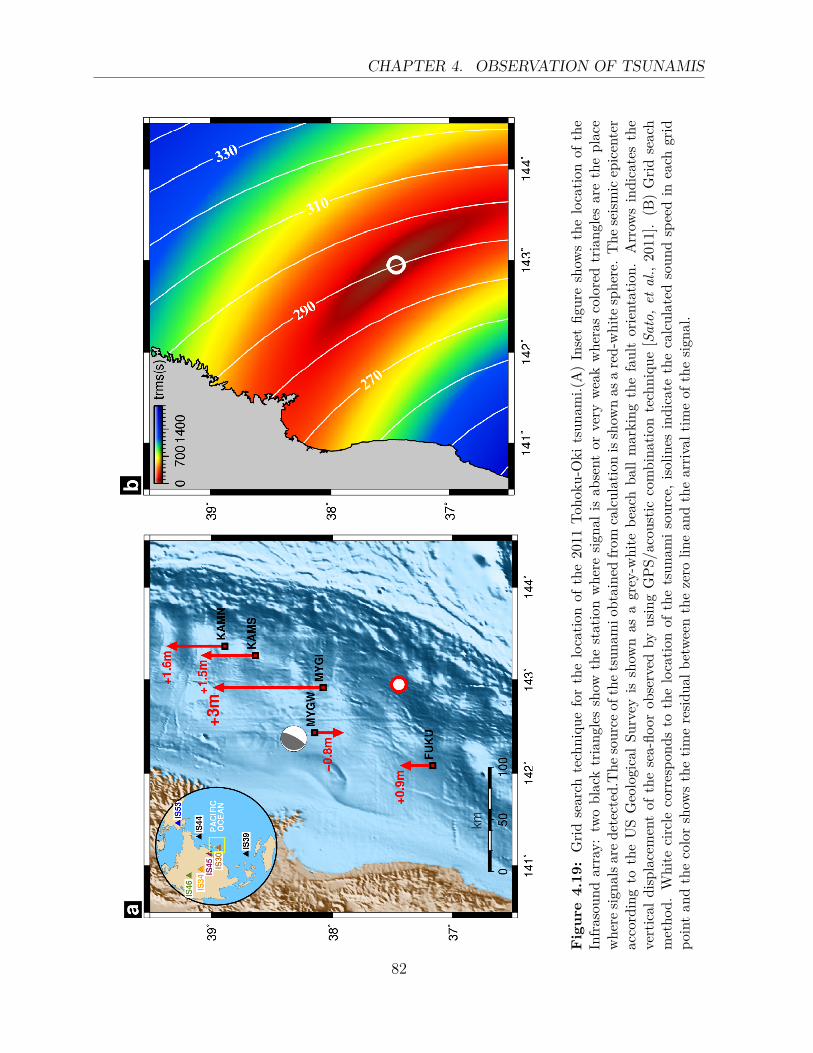
CHAPTER 4. OBSERVATION OF TSUNAMIS
Fig
ure
4.19
:G
ridse
arch
tech
niqu
efo
rth
elo
catio
nof
the
2011
Toho
ku-O
kits
unam
i.(A
)In
set
figur
esh
ows
the
loca
tion
ofth
eIn
fras
ound
arra
y:tw
obl
ack
tria
ngle
ssh
owth
est
atio
nw
here
signa
lis
abse
ntor
very
wea
kw
hera
sco
lore
dtr
iang
les
are
the
plac
ew
here
signa
lsar
ede
tect
ed.T
heso
urce
ofth
ets
unam
iobt
aine
dfr
omca
lcul
atio
nis
show
nas
are
d-w
hite
sphe
re.
The
seism
icep
icen
ter
acco
rdin
gto
the
US
Geo
logi
cal
Surv
eyis
show
nas
agr
ey-w
hite
beac
hba
llm
arki
ngth
efa
ult
orie
ntat
ion.
Arr
ows
indi
cate
sth
eve
rtic
aldi
spla
cem
ent
ofth
ese
a-flo
orob
serv
edby
usin
gG
PS/a
cous
ticco
mbi
natio
nte
chni
que
[Sat
o,et
al.,
2011
].(B
)G
ridse
ach
met
hod.
Whi
teci
rcle
corr
espo
nds
toth
elo
catio
nof
the
tsun
amis
ourc
e,iso
lines
indi
cate
the
calc
ulat
edso
und
spee
din
each
grid
poin
tan
dth
eco
lor
show
sth
etim
ere
sidua
lbet
wee
nth
eze
rolin
ean
dth
ear
rival
time
ofth
esig
nal.
82
4.2. INFRASOUND OBSERVATION OF TSUNAMIS
Fig
ure
4.20
:En
larg
edlo
catio
nm
apof
infr
asou
ndst
atio
ns.
Circ
les
indi
cate
the
poss
ible
sour
ceof
the
tsun
amif
orea
chst
atio
n.C
oord
inat
esof
the
tsun
amis
ourc
ean
dav
erag
ew
ave
spee
dof
the
tsun
amia
reth
efr
eepa
ram
eter
sin
the
grid
sear
ch.
The
tsun
ami
sour
ceis
estim
ated
tobe
atth
ein
ters
ectio
nof
allc
ircle
s.So
lidbl
uelin
ein
dica
tes
the
arriv
altim
eof
the
signa
lrec
orde
dat
Ala
skan
stat
ion
with
asp
eed
of29
0m
/sw
here
asda
shed
blue
line
isth
esa
me
signa
lwith
asp
eed
of35
6m
/s.
83
CHAPTER 4. OBSERVATION OF TSUNAMIS
Table 4.3: Infrasound signal observed at IMS stations for the 2011 Tohoku-Oki tsunami.
Stations Latitude Longitude Elevation Distance Speed Period(m) (◦) (m/s) (s)
IS30 35.31◦N 140.31◦E 52.0 3.02 288 604IS45 43.7◦N 131.9◦E NaN 10.46 290 560IS34 47.8◦N 106.41◦E 1288.0 28.56 290 516IS46 53.95◦N 84.82◦E NaN 42.54 290 628IS53 64.87◦N 147.86◦W 200.0 48.06 356 848
traveling time. The location of the source will be the area where circular zone of three
or more stations intersect at the same location. As a result, the Asian station intersects
at 37.45 ◦N, 142.95 ◦E with a speed of 290 m/s whereas the Alaskan needs 356 m/s to
reach the same location (dashed blue line). Delays of the tsunami origin time relative to
the earthquake origin time by up to 100s changed the location of the tsunami source by
less than 50km.
Figure 4.21: Black trace shows station where there was no signal. Alaskan station (blue) istaken as reference. The red and green marks indicate speeds of 356 and 290m/sec, respectively.Zero time corresponds to a speed of 310m/sec. A weak indication for a signal traveling with aspeed of 330m/sec is marked in black at station IS44.
Figure 4.21 shows the infrasound records of the stations IS39 and IS44 in comparison with
the station IS53 in Alaska. Zero time of the traces indicates the arrival time of a possible
84
4.2. INFRASOUND OBSERVATION OF TSUNAMIS
signal traveling with a speed of 310m/sec. In our search, we fail to detect signal traveling
with a speed of 356 and 290m/sec indicated by red an green marks respectively. A very
weak signal traveling with a speed of 330 m/s may be detected at station IS44, which has
a similar backazimuth like the Alaskan station. No signal is detectable above the noise
level at station IS39 in the western Pacific, which has a backazimuth nearly opposite to
the Alaskan station. This might be an effect of source directivity.
4.2.4.3 Discussion
The location of the tsunami source obtained by using this technique is reasonably accept-
able. Note that the largest observed GPS ground displacement and the tsunami source
are all located within about 100km of each other and the seismic epicenter is also within
the same area. It indicates that the Tohoku-Oki earthquake has generated dislocations of
the sea surface in the epicentral region of the earthquake, which acted as source of ultra
long period infrasound signals. Thus, infrasound source region is also the source region
of the tsunami and the region with largest vertical displacements of the sea bottom. The
common velocities of infrasound are near 300m/s with variations of ±50m/s due to wind
speed [Arrowsmith et al 2010]. Here we observe for the Asian stations 290m/s and for the
Alaskan station 356m/s. This could be explained by a strong wind component blowing in
the opposite direction of the propagating infrasound to all Asian stations. For the Alaskan
station a wind of about the same speed but in the same direction as the infrasound would
increase its infrasound speed. Data from a larger number of better distributed and closer
infrasound stations would certainly increase the accuracy of the location of the infrasound
source. Therefore, real-time processing of infrasound observations may improve tsunami
modeling for early warning purposes. Assuming an average water depth of 1000m, the
speed of the tsunami is about three times less than the speed of infrasound. This means
a tsunami needs about 15 minutes to reach a coast 100km away from the epicenter. The
85
CHAPTER 4. OBSERVATION OF TSUNAMIS
infrasound signal of the tsunami already indicates 5 minutes after the origin time that a
tsunami is definitely coming. From the size and the regional distribution of the infrasound
signals a better modeling of the tsunami arriving at the shores may be obtained.
86
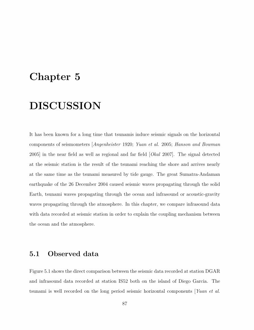
Chapter 5
DISCUSSION
It has been known for a long time that tsunamis induce seismic signals on the horizontal
components of seismometers [Angenheister 1920; Yuan et al. 2005; Hanson and Bowman
2005] in the near field as well as regional and far field [Okal 2007]. The signal detected
at the seismic station is the result of the tsunami reaching the shore and arrives nearly
at the same time as the tsunami measured by tide gauge. The great Sumatra-Andaman
earthquake of the 26 December 2004 caused seismic waves propagating through the solid
Earth, tsunami waves propagating through the ocean and infrasound or acoustic-gravity
waves propagating through the atmosphere. In this chapter, we compare infrasound data
with data recorded at seismic station in order to explain the coupling mechanism between
the ocean and the atmosphere.
5.1 Observed data
Figure 5.1 shows the direct comparison between the seismic data recorded at station DGAR
and infrasound data recorded at station IS52 both on the island of Diego Garcia. The
tsunami is well recorded on the long period seismic horizontal components [Yuan et al.
87
CHAPTER 5. DISCUSSION
2005].
Figure 5.1: Comparison of seismic and infrasound records at Diego Garcia.(Filter used arewritten above the trace)A(top): Seismic (red) and infrasound (blue) data zoomed between the first 30 min. B(bottom):(red) Long period filtered three-component seismic data. TS indicates the tsunami arrival andIS marks the infrasound arrival, (blue) Filtered infrasound data, gray traces are the duplicate ofthe infrasound blue trace.
By comparing the two traces recorded from two different types of instruments, the seismic
and infrasound data in Figure 5.1-A show a nearly one to one agreement for the first half
hour after the origin time of the Sumatra-Andaman earthquake. Watada et al. (2006)
showed similar observations while analyzing the M8.3 Tokachi-Oki, Japan earthquake in
2003. This is an indication of the existing coupling between solid earth and the atmosphere.
However, the coupling is not a total and the system where the phenomenon occurs is very
complex. Therefore, we initially assumed that the good correlation between two traces in
88
5.2. SYNTHETIC DATA
the first half an hour could be partially caused by mechanical effect of the ground shaking
during the passage of the seismic wave on the instrument.
Figure 5.1B shows different long period signal detectable not only on infrasound data
(blue) but also on the three (vertical, radial and transversal) components of the seismic
data (red). Therefore different type of filters are applied to each component. For the
infrasound data, a second order high-pass Butterworth filter with a corner frequency of
800s is applied. The small box on the infrasound trace indicates the seismic phase which is
zoomed on Figure 5.1A. The arrival of the infrasound caused by the tsunami is marked ”IS”.
We applied different filters for the seismic data. The vertical component is band-pass
filtered by second order Butterworth with corner frequencies 200 s and 600 s. The Rayleigh
wave groups traveling around the globe is observed on the filtered vertical component which
starts nearly at 02:20 (UT) and stops at 04:30 (UT). An indication of long period signal is
observed on infrasound trace which may correspond to this passage. No clear infrasound
signal is identified at the arrival time of the tsunami. However, on the two horizontal
components, a very clear signal related to the tsunami arrival time is observed and marked
”TS”. This is a confirmation of several similar observations, as mentioned in chapter 3,
that seismometer horizontal components respond to the loading effect of the tsunami.
5.2 Synthetic data
Similarly to the comparison done with the observed data, Figure 5.2 shows the theoretical
trace of both seismic and infrasound data. Thus, we compared a waveform of about 30
minutes length [Figure 5.2A]. The zero time of the trace corresponds to the origin time
of the earthquake. A perfect agreement between both types of data is noticed up to
89
CHAPTER 5. DISCUSSION
about 01:17 UT. This good correlation confirms that the near-perfect agreement between
observed seismic and infrasound signals in Figure 5.1A is largely caused by coupling of
solid Earth to atmosphere. Note that no instrument effect is introduced on the calculation
of the theoretical trace. The amplitude scale of the signal does not have any physical
meaning however we noticed that the ratio of the two traces is 5 Pa/(cm/s) which is
exactly similar to what is observed data in Figure 5.1A. This indicates that the entire
observed infrasound signal (Figure 5.1A) is indeed caused by leaking of seismic energy into
pressure changes in the atmosphere. Shaking of the microbarograph does not contribute
much to the infrasound record.
The theoretical seismic and infrasound records up to 01:17 UT agree very well. After that
time we obtain strong infrasound signals predicted by the model but we do not observed
similar signal in the recorded data. We interpret this signal as a vertical reflection of
the waves, generated by the passage of seismic surface wave at the infrasound station, in
the atmosphere and do not propagate horizontally. Their amplification may be caused
by insufficient attenuation in the atmosphere of our model. We used in the atmosphere
a quality factor Q of 100. Test computations with larger Q values increased the ringing
effects drastically. The Q factor used here must be understood not necessarily as the usual
Q caused by friction. It also represents attenuations caused by lateral heterogeneities and
has therefore no physical meaning.
In Figure 5.2B the infrasound signal of the tsunami and also the tsunami effect on the
seismometers is relatively well reproduced. The absence of any signal on the transverse
component of the theoretical seismograms is due to the fact that the calculation is done
for a point source. However, the radial component detects well the arrival of the tsunami
at shore.
90
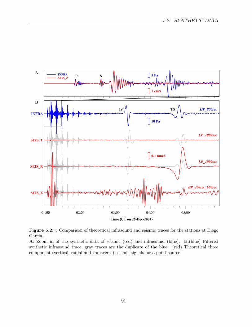
5.2. SYNTHETIC DATA
Figure 5.2: : Comparison of theoretical infrasound and seismic traces for the stations at DiegoGarcia.A: Zoom in of the synthetic data of seismic (red) and infrasound (blue). B:(blue) Filteredsynthetic infrasound trace, gray traces are the duplicate of the blue. (red) Theoretical threecomponent (vertical, radial and transverse) seismic signals for a point source
91
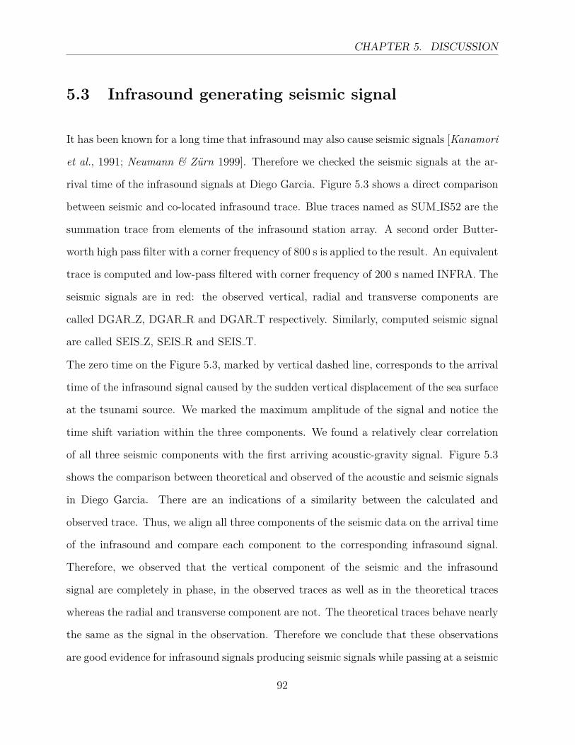
CHAPTER 5. DISCUSSION
5.3 Infrasound generating seismic signal
It has been known for a long time that infrasound may also cause seismic signals [Kanamori
et al., 1991; Neumann & Zürn 1999]. Therefore we checked the seismic signals at the ar-
rival time of the infrasound signals at Diego Garcia. Figure 5.3 shows a direct comparison
between seismic and co-located infrasound trace. Blue traces named as SUM IS52 are the
summation trace from elements of the infrasound station array. A second order Butter-
worth high pass filter with a corner frequency of 800 s is applied to the result. An equivalent
trace is computed and low-pass filtered with corner frequency of 200 s named INFRA. The
seismic signals are in red: the observed vertical, radial and transverse components are
called DGAR Z, DGAR R and DGAR T respectively. Similarly, computed seismic signal
are called SEIS Z, SEIS R and SEIS T.
The zero time on the Figure 5.3, marked by vertical dashed line, corresponds to the arrival
time of the infrasound signal caused by the sudden vertical displacement of the sea surface
at the tsunami source. We marked the maximum amplitude of the signal and notice the
time shift variation within the three components. We found a relatively clear correlation
of all three seismic components with the first arriving acoustic-gravity signal. Figure 5.3
shows the comparison between theoretical and observed of the acoustic and seismic signals
in Diego Garcia. There are an indications of a similarity between the calculated and
observed trace. Thus, we align all three components of the seismic data on the arrival time
of the infrasound and compare each component to the corresponding infrasound signal.
Therefore, we observed that the vertical component of the seismic and the infrasound
signal are completely in phase, in the observed traces as well as in the theoretical traces
whereas the radial and transverse component are not. The theoretical traces behave nearly
the same as the signal in the observation. Therefore we conclude that these observations
are good evidence for infrasound signals producing seismic signals while passing at a seismic
92
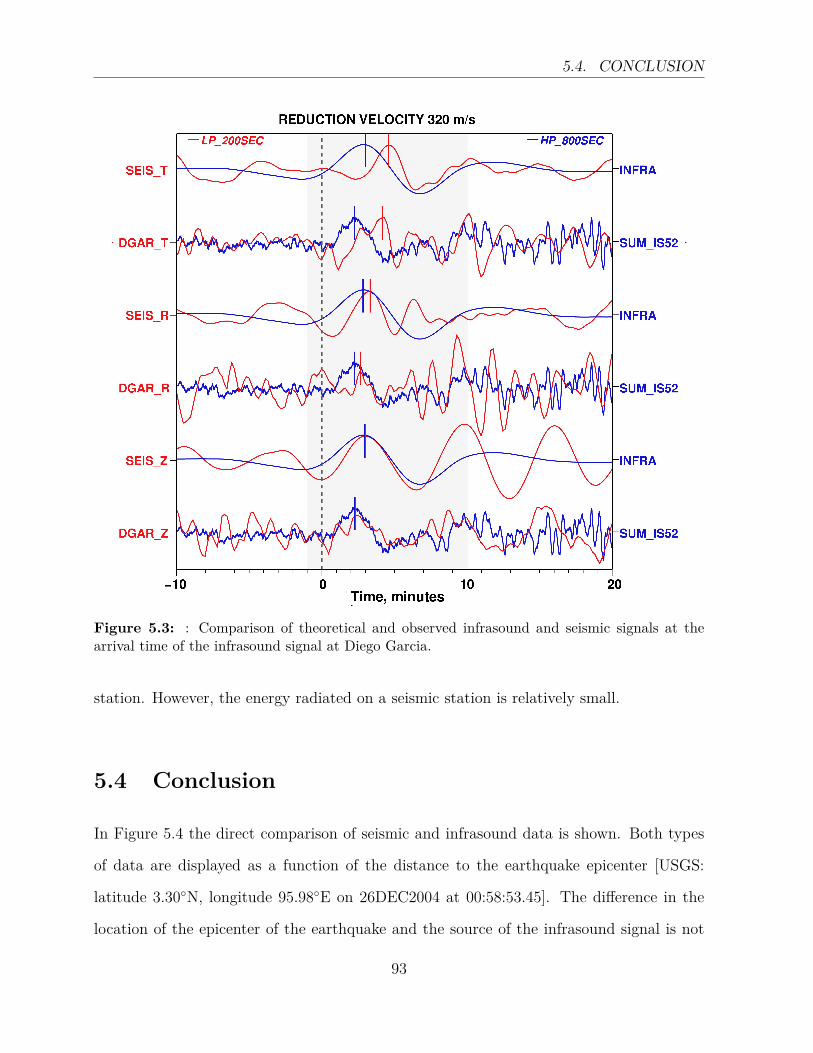
5.4. CONCLUSION
Figure 5.3: : Comparison of theoretical and observed infrasound and seismic signals at thearrival time of the infrasound signal at Diego Garcia.
station. However, the energy radiated on a seismic station is relatively small.
5.4 Conclusion
In Figure 5.4 the direct comparison of seismic and infrasound data is shown. Both types
of data are displayed as a function of the distance to the earthquake epicenter [USGS:
latitude 3.30◦N, longitude 95.98◦E on 26DEC2004 at 00:58:53.45]. The difference in the
location of the epicenter of the earthquake and the source of the infrasound signal is not
93
CHAPTER 5. DISCUSSION
considered in this figure. The seismic data show clearly a wave traveling with a velocity of
about 203 m/s, which is a tsunami velocity. These waves have been observed by Yuan et
al. (2005) and interpreted as effect of tilted ocean islands or ocean shores caused by the
tsunami. The infrasound data shows a phase traveling with a velocity of about 320 m/s.
The usual seismic phases are traveling with much faster velocity.
We have confirmed that the first arriving acoustic-gravity signal may originate from the
tsunami source region that is the region of great changes of the sea level caused by changes
of the sea floor due to the earthquake. Therefore these signals can be used for tsunami
early warning purposes. Acoustic-gravity waves are usually recorded at microbarograph
stations. We have shown that acoustic-gravity waves may also be recorded at seismic
broadband stations. There exist usually more seismic stations than infrasound stations,
therefore such stations may be supplemented by the large number of seismic stations in
tsunami warning systems. It is known that seismic stations at ocean islands or coastal
regions behave similarly to tide gauges or DART buoys and record tsunami. Now it seems
useful to develop technique of scanning seismic data in order to identify an indications of
infrasound signals radiated from the tsunami source region which arrive earlier than the
tsunami and to use this information for early warning purposes.
The observation made for Tohoku-Oki event in Japan confirms that the sudden vertical
displacement of the sea surface at the tsunami source produces a very long period acoustic
gravity signal in the atmosphere. Infrasound station, designed to detect nuclear explosion
in the atmosphere, can clearly detect such signal. The solution from our grid search of
the minimum value of the residual time demonstrated the possible location of the tsunami
source in an ellipse nearly perpendicular to the direction of the trench.
94
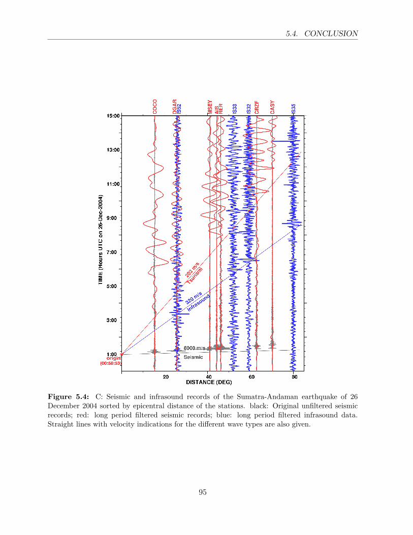
5.4. CONCLUSION
Figure 5.4: C: Seismic and infrasound records of the Sumatra-Andaman earthquake of 26December 2004 sorted by epicentral distance of the stations. black: Original unfiltered seismicrecords; red: long period filtered seismic records; blue: long period filtered infrasound data.Straight lines with velocity indications for the different wave types are also given.
95
Chapter 6
Summary and Outlook
The aim of this work was to find an additional set of data which can provide additional
information of evidence of tsunami following a great earthquake. This work demonstrates
that seismometers can be very sensitive to the passage of tsunami for seismic stations
deployed on oceanic island within distance less than 100km away from the shore line.
Therefore, by applying a third order band pass Butterworth filter with a corner frequency
between 1 mHz and 10 mHz, a very clear evidence of tsunami (large SNR) with a period
of ≈ 30min was observed on the horizontal component of the seismometer. The seismic
data show clearly a wave traveling with a velocity of about 203 m/s, which corresponds to
the average velocity of a tsunami. For the station located on an island close to close to a
continental boundary, combination of the multiple wave reflected from the continent and
the effect of the shallow bathymetry are involved in the signal and the speed of the wave
decreased. Comparison of signal observed on seismometer with data form nearby DART
and tide gage stations demonstrate that seismometers respond to tsunami and can be used
as a tsunameter. This can be advantageous for tsunami monitoring because seismic sta-
tions are located inland i.e. safe from any damage caused by the tsunami itself and free
from local effect of the geometry of the local harbor.
96
The second dataset analyzed for tsunami detection in this study is infrasound. Initially,
infrasound station installed by CTBTO, Vienna are designed to detect nuclear explosion in
the atmosphere but since tsunami can excite the atmosphere due to the coupling effect, we
were motivated to investigate tsunami signals on infrasound data. In this part, we focused
on infrasound signals generated by a tsunami around the source itself. After analysis of
data from IMS/CTBTO we have confirmed that the sudden vertical displacement of the
sea surface at the tsunami source produces a very long period acoustic gravity signal in the
atmosphere. The first arriving acoustic-gravity signal recorded at an infrasound station
originates from the tsunami source region that is the region of great changes of the sea level
caused by changes of the sea floor due to the earthquake. This location of the tsunami
source obtained by using infrasound data corresponds to the largest coseismic slip obtained
from GPS data analysis. It is somewhat located within about 100km from the maximal
vertical displacement. In this study, we deducted that the velocity of the acoustic-gravity
wave detected in the infrasound data travels near 300m/s with variations of ±50m/s.
In chapter 5, we compare the seismic and infrasound data fro the Sumatra-Andaman event.
For the first half an hour after the earthquake, a good agreement is found between these
two data set. This might be caused by a mechanical effect of the shaking on the instrument.
Besides, the same correlation between seismic and infrasound data was also found by doing
comparison of theoretical data in which no instrument effect was introduced. The second
observation from synthetic data demonstrates that earth-atmosphere coupling is also in-
volved. Data from Diego Garcia shows an evidence of acoustic-gravity waves recorded at
seismic station.
We have shown also that the infrasound signal travels faster than the seismic so infrasound
97
CHAPTER 6. SUMMARY AND OUTLOOK
can not only be used for tsunami early warning purposes but it can be used for tsunami
source location which might help tsunami modelers for the initial condition of their run.
As explained in this thesis, infrasound station can detect long period signal generated by
tsunami. Therefore, in order to get a good coverage of data, it might be a task of future
work to increase a number of infrasound station in the area close to a potential source of
tsunami. As described before, location of the tsunami source was based on the empirical
method of circle intersection used by seismologist. This implies that many simplification
was applied during this study which need to be corrected. This may improve not only the
location of the tsunami source but also a better estimation of the acoustic gravity wave
speed.
Observation from one station indicated the presence of an acoustic gravity wave on seismic
broadband station. Therefore, it might also be important to investigate more in detail these
signal on seismic broadband station since there exist more seismic station than infrasound
station deployed all around the world. Infrasound would be supplemented by the large
number of seismic station in tsunami warning system.
98
Bibliography
Abe, K. (1973). Size of great earthquakes of 1873 - 1974 inferred from tsunami data. J.
Geophys. Res., 84, 1561 - 1568.
Abe, K. (1973). Tsunami and mechanism of great earthquakes, Phys. Earth. Planet.
Inter. 7, 143 – 153.
Abe, K. (1988). Tsunami magnitude and the quantification of earthquakes tsunamis around
Japan. Bull. Earthquake Res. Inst. Univ. Tokyo. 63,289 - 303.
Abe, K. (2007). Phases representing source Lengths of tsunami in Tide gauge records.
Pure appl.geophys.. 164,453-463.
Afraimovich E.L., et al. (2001). The shock-acoustic waves generated by earthquakes, An-
nales Geophysicae,19 395-409.
Angenheister, G. (1920). Vier Erdbeben und Flutwellen im Pazifischen Ozean, beobachtet
am Samoa- Observatorium, 1917-1919. Nachrichten von der Gesellschaft der Wissenschaften
zu Göttingen, 201-204.
Arendt, S., & Fritts, D. (2000). Acoustic radiation by ocean surface waves, J. Fluid.
Mech.,415, 1-21.
99
BIBLIOGRAPHY
Artru, J., V. Ducic, H. Kanamori, Ph. Lognonne and M. Murakami (2005), Ionospheric
detection of gravity waves induced by tsunamis, Geophys. J. Int., 160, 840 - 848.
Arrowsmith, S. J., J. B. Johnson, D. P. Drob, and M. A. H. Hedlin (2010), The seismoa-
coustic wavefield: a new paradigm in studying geophysical phenomena, Rev. Geophys.,48
RG4003.
Bilham, R., E .R. Engdahl, N. Feldl and S. P. Satyabala (2005), Partial and complete rup-
ture of the Indo-Andaman plate boundary 1847- 2004, Seismol. Res. Lett., 76, 299-311.
Blanc, E. (1985). Observations in the upper atmosphere of infrasonic waves from natural
or artificial sources: A summary, Ann. Geophys., 3, 673-688.
Boris, L., & Mikhail, N. (2009). Physics of tsunamis. Springer, Netherlands.
Brachet N., Brown D., Le Bras R., Mialle P., Coyne J. (2010). Monitoring the earth′s at-
mosphere with the global IMS infrasound network. Atmospheric variability and infrasound
monitoring, Springer,73 – 114.
Calais, E., Minster J.B., Michelle A.H. & Hedlin, M.(1998). Ionospheric signature of sur-
face mine blasts from Global. Positioning System measurements. Geophys. J. Int.,132,
191-202.
Clinton, John F. (2004) Modern digital seismology - instrumentation, and small amplitude
studies in the engineering world. Dissertation (Ph.D.), California Institute of Technology.
Comer, R.P. (1980). Tsunami height and earthquake magnitude: theoretical basis of an
empirical relation. Geophys. Res. lett., 7, 445 - 448.
Daniels, Fred B.(1952). Acoustical Energy Generated by the Ocean Waves, J. Acoust. Soc.
100
BIBLIOGRAPHY
Am., 24, 83-83 .
Degg, M. and Doornkamp, J.C. (1994). Earthquake hazard Atlas: 7 Iberia (Portugal and
Spain) including the Azores: Balearics, Canary and Madeira Islands. London: London
Insurance and Reinsurance Market Association.
Dotsenko, S.F., Kuzin, I.P., Levin, B.V., Solov’eva O.N. (2000). Tsunami in the Caspian
sea: Seismic sources and features of propagation. Oceanology, 40. 474 - 482.
Ducic, V., Artru, J. & Lognonné P.(2003)Ionospheric remote sensing of the Denali Earth-
quake Rayleigh surface waves. Geophys. Res. Lett.,30, 1951.
Dutykh, D., Dimitrios, D., Chubarov, L.,Shokin, Y. (2011) The contribution of horizontal
sea-bed displacements into tsunami generation processes.
http://arxiv.org/abs/1002.3019.,12.
Eric, B. K., Joost, A. B. (1994). Atmosphere-Ocean Interaction, Second Edition, Oxford
monographs on geology and geophysics N 27, ISBN 019 506618 9 Earl, E.G., William
H. (1975). Wave in the atmosphere: Atmospheric Infrasound and Gravity waves. Their
generation and propagation, Library of Congress Card Number: 73 89155, 0 444 41196
8 Fine, I. V., Rabinovich A. B. & Thomson R. E. (2005), The dual source region for the
2004 Sumatra tsunami, Geophys. Res. Lett., 32, L16602.
Fitzgerald, T.J. (1997). Observations of total electron content perturbations on GPS sig-
nals caused by a ground level explosion. J. of Atm. & Solar-Terrestrial Phys. 59, 829-834
.
Francis, P. W.(1985). The origin of the 1883 Krakatau tsunamis. J. Volcanol.Geotherm.
Res., 25, 349 369.
101
BIBLIOGRAPHY
Garces, M.,Hetzer, Claus., Businger, S., & Willis M. (2002). Modeling of microbarom sig-
nals in the Pacific. paper presented at the 24th Seismic Research Review Nuclear Explosion
Monitoring: Innovation and Integration.
Garces, M., P. Caron, C. Hetzer, A. Le Pichon, H. Bass, D. Drob & Bhattacharyya J.
(2005). Deep Infrasound Radiated by the Sumatra Earthquake and Tsunami. Eos Trans.
AGU, 86, 317-319.
Geller, R.J. (1976). Sacling relations for earthquake source parameters and magnitudes.
Bull. Seismol. Soc. Am., 66, 1501 - 1523.
Gilbert, F. (1980) An introduction to low-frequency seismology. In Proc. Intl. School
Phys. ”Enrico Fermi”, (eds. A.M. Dziewonski and E. Boschi), 78, 41 81 (North Holland,
Amsterdam, 1980).
Gilbert, F. & Backus G. (1968). Elastic-gravitational vibrations of a radially stratified
sphere, in Dynamics of Stratified Solids. American Society of Mechanical Engineers, New
York, 82-95.
Gladwin, M.T., Gwyther, R.L., Hart, R., Francis, M., Johnston, M.J.S. (1987). Borehole
tensor strain measurements in California. J. Geophys. Res., 92, 7981 7988.
Gonzalez, F.I., Milburn, H.M., Bernard, E.N. and Newman, J.C. (1998). Deep-ocean
Assessment and Reporting of Tsunamis (DART): Brief Overview and Status Report. In
Proceedings of the International Workshop on Tsunami Disaster Mitigation, 19-22 January
1998, Tokyo, Japan. Retrieved September 20, 2005.
http://www.pmel.noaa.gov/tsunami/dart report1998.html
Hanson, J.A. & Bowman, J., R. (2005). Dispersive and reflected tsunami signals from the
102
BIBLIOGRAPHY
2004 Indian Ocean tsunami observed on hydrophones and seismic stations. Geophys. Res.
Lett17, L17606.
Harbitz, C.B., Lovholt, F., Pedersen, G., & Masson, D.G. (2006). Mechanisms of tsunami
generation by submarine landslides: a short review. Norwegian Journal of Geology, 86,
255-264.
Hakrider, D., Press, F. (1967). The krakatoa Air-Sea Waves: an example of pulse propa-
gation in coupled systems. Geophys. J. R. astr. Soc., 13, 149-159.
Harkrider,David G., Newton,Carl A. & Flinn,Edward A. (1974). Theoretical Effect of Yield
and Burst Height of Atmospheric Explosions on Rayleigh Wave Amplitudes. Geophys. J.
R. astr. Soc., 36, 191-225.
Hatori, T. (1979). Relation between tsunami magnitude and wave energy. Bull. Earthq.
Res. Inst. Univ. Tokyo, 54, 131 - 541.
Hébert, H., Heinrich, P., Schindelé, F., and Piatanesi, A. (2001). Far-field simulation of
tsunami propagation in the Pacific Ocean: impact on the Marquesas Islands (French Poly-
nesia). J. Geophys. Res., 9161 - 9177.
Heki, K.,Otsuka Y. , Choosakul N., Hemmakorn N., Komolmis T. & Maruyama T. (2006)
Detection of ruptures of Andaman fault segments in the 2004 great Sumatra earthquake
with coseismic ionospheric disturbances. J. Geophys. Res., 111, B09313.
Hidayat, D., Voight, B., Langston, C., Ratdomopurbo, A. & Ebeling, C. (2000). Broadband
seismic experiment at Merapi Volcano, Java, Indonesia: very-long-period pulses embedded
in multiphase earthquakes, J. Volc. Geotherm. Res., 100, 215 231.
103

BIBLIOGRAPHY
Iida K., Cox, D.C., Pararas-Carayannis, G. (1967). Preliminary catalog of tsunami occur-
ring in the Pacific Ocean. Data Report No. 5, HIG-67-10. University of Hawaii, Hnolulu.
Isaac V. Fine, Josef Y. Cherniawsky, Alexander B. Rabinovich, Stephenson F.(2009). Nu-
merical modeling and observations of tsunami waves in Alberni Inlet and Barkley Sound,
British Columbia. Pure appl. geophys., 165, 2019 2044.
Jacques, V. M. and Soloviev,S. L. (1971). Distant registration of small waves of tsunami
type on the shelf of the Kuril. Islands, Dok. Akad. Nauk USSR, 198, 816-817.
Ji, C. (2005), Magnitude 9.0 earthquake off the west coast of northern Sumatra: Prelimi-
nary rupture model, report, U.S. Geol. Surv., Denver, Colo.
http://neic.usgs.gov/neis/eq depot/2004/eq 041226/neic slav ff.html.
Kajiura, K. (1963). The leading wave of a tsunami. Bull. Earthquake Res. Inst., 41, 535
571.
Kajiura, K. (1970). Tsunami source, energy and the directivity of wave radiation. Bull.
Earthquake Res. Inst., 48, 835 869.
Kanamori, H. (1972). Mechanism of tsunami earthquakes, Phys. Earth Planet. Int., 6,
246 259.
Kanamori, H. J. Mori, D.L. Anderson & T.H. Heaton (1991). Seismic excitation by the
space shuttle Columbia. Nature, 349, 781 782.
Kulichkov, S., N. (2004). Long-range propagation and scattering of low-frequency sound
pulses in the middle atmosphere. Meteorol. Atmos. Phys., 85, 47 60.
Kulichkov, S. N., Chunchuzov, I. P., Bush, G. A., & Perepelkin, V. G. (2008). Physical
104
BIBLIOGRAPHY
modeling of long-range infrasonic propagation in the atmosphere. Izvestiya Atmospheric
and Oceanic Physics, 44, 175 186.
Kong, L. (2004).Scientists hope to save more lives by learning better ways to predict
the approach of killer waves.SCIENCE YEAR, The World Book Annual Science Supple-
ment(http://ioc3.unesco.org/itic/files/worldbook tsunami.pdf)
Lander, J.F., Whiteside, L.S., Lockridge, P.A. (2002). A brief history of tsunami in the
Caribbean Sea. Sci. Tsunami Hazards, 20.
La Rocca, M., Galluzzo, D., Saccorotti, G., Tinti, S., Cimini, G.B., and Del Pezzo E.
(2004), Seismic signals associated with landslides and with a tsunami at Stromboli Vol-
cano, Italy. Bull. Seismol. Soc. Amer., 94, 1850 1867.
Lay T., H. Kanamori, C.J. Ammon, M. Nettles, S.N. Ward, R.C. Aster, S.L. Beck, S.L.
Bilek, M.R. Brudzinski, R. Butler, H.R. DeShon, G. Ekstrom, K. Satake & Sipkin S. (2005).
The great Sumatra-Andaman earthquake of 26 December 2004. Science, 308, 1127-1133.
Le Pichon, A., Maurer, V., Raymond, D., & Hyvernaud, O. (2004). Infrasound from ocean
waves observed in Tahiti. Geophys. Res. Lett.,31, L19103.
Le Pichon, A., P. Herry, P. Mialle, J. Vergoz, J. Brachet, N. Garces, D. Drob & Ceranna
L. (2005), Infrasound associated with 2004-2005 large Sumatra earthquakes and tsunami.
Geophys. Res. Lett., 19, L19802.
Longuet-Higgins, M. (1950). A theory of the origin of microseisms. Phil, Trans. Royal
Soc. London, Series A., Mathematical and Physical Sciences,243,1-35.
Lognonné, P., Clévédé C., & Kanamori H. (1998). Normal mode summation of seismo-
105
BIBLIOGRAPHY
grams and barograms in an spherical Earth with realistic atmosphere. Geophys. J. Int.,
Geophys. J. Int., 135, 388-406.
Meltzner, A. J. et al. (2006) Uplift and subsidence associated with the great Aceh-
Andaman earthquake of 2004. J. Geophys. Res.,111, 02407
Mikumo, T., T. Shibutani, A. Le Pichon, M. Garces, D. Fee, T. Tsuyuki, S. Watad & Morii
W.(2008), Low-frequency acoustic-gravity waves from coseismic vertical deformation asso-
ciated with the 2004 Sumatra-Andaman earthquake (M-w=9.2), J. Geophys. Res., 113,
B12402.
Nagarajan, B., Suresh, I., Sundar D., Sharma R., Lal, A. K., Neetu, S. , Shenoi, C., Shetye,
S., R. and Shankar, D. (2006). The Great Tsunami of 26 December 2004: A description
based on tide-gauge data from the Indian subcontinent and surrounding areas. Earth Plan-
ets Space, 58, 211 215.
Neumann, U. & Zürn W. (1999). Gravity signals from atmospheric waves and their mod-
eling, Bull. Inf. Marees Terr., 131, 10,139-10,152.
Nishida, K., Kobayashi, N., & Fukao Y.(2000). Resonant Oscillations Between the Solid
Earth and the Atmosphere.Science, 287, 2244.
Nikonov, A.A. (1997). Tsunami occurrence on the coasts of the Black Sea and the Sea of
Azov. Izv.Phys.Solid Earth, 33, 72 - 87.
Nosov M. A. (1998). Tsunami generation in compressible ocean.Phys. Chem. Earth
(B),24, 437-441.
Ohmachi, T., Inoue, S., Matsumoto, H., Tsukiyama, H. (2001). Tsunami simulation tech-
106
BIBLIOGRAPHY
nique considering dynamic seabed displacement and acoustic effects of water. Int. Tsunami
Symp., session 7, 7-8.
Okal, E.A., and Titov, V. (2007). MTSU: Recovering seismic moments from tsunameter
records. Pure Appl. Geophys.,164, 355 - 378.
Okal E. A. (2007). Seismic Records of the 2004 Sumatra and Other Tsunamis: A Quanti-
tative Study. Pure appl. geophys., 64, 325 353 .
Osler, J. C., & Chapman, D. M. F. (1998). Quantifying the interaction of an ocean bottom
seismometer with the seabed. J. Geophys. Res., 103(B5), 9879 9894.
Posmentier, E. (1967). A Theory of Microbaroms. Geophys. J. R. Astr. Soc., 13, 487-501.
Piatanesi, A., & Lorito S. (2007), Rupture process of the 2004 Sumatra-Andaman Earth-
quake from Tsunami waveform inversion, Bull. Seismol. Soc. Am., 97, 223 231.
Rabinovich, A., & RICHARD, E. (2007).The 26 December 2004 Sumatra Tsunami: Anal-
ysis of Tide Gauge Data from the World Ocean Part 1. Indian Ocean and South Africa.
Pure appl. geophys., 164, 261 308
Rhie J., & Romanowicz B. (2004). Excitation of Earth’s continuous free oscillations by
atmosphere ocean seafloor coupling. Nature, 431, 552-556.
Rodgers P. W. (1968). The response of the horizontal pendulum seismometer to Rayleigh
waves, Love waves, tilt, and free oscillations of the Earth, Bull. Seism. Soc. Am., 58,
1384-1406.
Saito, T., & Furumura T. (2009), Three-dimensional simulation of tsunami generation and
propagation: Application to intraplate events, J. Geophys. Res., 114.
107
BIBLIOGRAPHY
Sato M.,Ishikawa T.,Ujihara N., Yoshida S., Fujita M., Mochizuki M., Asada A.(2011).
Displacement Above the Hypocenter of the 2011 Tohoku-Oki Earthquake. Science, 332,
1395.
Song, Y. T., C. Ji, L.-L. Fu, V. Zlotnicki, C. K. Shum, Y. Yi, & Hjorleifsdottir V. (2005),
The 26 December 2004 tsunami source estimated from satellite radar altimetry and seismic
waves, Geophys. Res. Lett., 32, L20601.
Self, S., & Rampint,M., R. (1981) The 1883 eruption of Krakatau, Nature,294, 699-704.
Sigurdsson, H.; Carey, S.; Mandeville, C.; Bronto, S. (1991). Pyroclastic flows of the 1883
Krakatau eruption. EOS 72, 36, 377-381.
Simon, D., Schneider, M.M. (1967). Zum Auftreten luftdruckbedingter Storungen in Hori-
zontalpendelaufzeichnungen auf drei verschiedenen Erdgezeitenstationen. B.I.M., 49, 2218
2225.
Soloviev, S.L., Go C.N., Kim Kh.S. (1986). Catalogue of tsunamis in the Pacific ocean,
1969-1982. Izd. MGK, USSR AS, Moscow.
Soloviev, S.L. (1970). Recurrence of tsunamis in the Pacific. In: ”Tsunamis in the Pacific
Ocean”, East-West Center Press, Honolulu, 149 - 164.
Subarya C., Chlieh M., Prawirodirdjo L., Avouac J.P., Bock Y., Sieh K., Meltzner A. J.,
Natawidjaja D. H. & McCaffrey R. (2006).Plate-boundary deformation associated with the
great Sumatra Andaman earthquake.nature, 440, doi:10.1038/04522 Takeuchi, H. & Saito
M. (1972), Seismic surface waves, in Methods in Computational Physics, pp. 217-295, ed.
Bolt, B. A., Academic Press, New York.
108
BIBLIOGRAPHY
Tanioka, Y., & Seno T. (2001), Sediment effect on tsunami generation of the 1896 Sanriku
tsunami earthquake, Geophys. Res. Lett., 28, 3389 3392.
Tinti, S., Bortolucci, E. & Chiavettieri, C. (2001). Tsunami Excitation by Submarine
Slides in Shallow-water Approximation. Pure Appl.Geophys., 158, 759 797.
Tinti, S., Maramai A., and Graziani L.. (2004). The New Catalogue of Italian Tsunamis .
Nat. Haz., 33, 439-465.
Titov, V. V, Mofjeld, H. O., Gonzalez, F. I., and Newman, J. C. (1999). Offshore forecast-
ing of Alaska-Aleutian subduction zone tsunamis in Hawaii. NOAA Tech. Memorandum,
ERL PMEL-114, PMEL, Seattle, WA, 22
Yamashita, T., & Sato R. (1974). Generation of tsunami by a fault model. J. Phys. Earth,
22, 415 440.
Yanagisawa, M., and T. Wakasugi (1984). Observations of crustal tilt and strain indeced
by the load of the 1983 Nihonkai-Chubu Earthquake tsunami. J. Geod. Soc. Jpn.30 ,
3,204 212.
Yokoyama, I. (1981) A geophysical interpretation of the 1883 Krakatau eruption, J. Vol-
canol. Geotherm. Res.,9, 359-378.
Yokoyama, I. (1987) A scenario of the 1883. Krakatau tsunami, J. Volcanol. Geotherm.
Res.,34, 123-132.
Yuan, X. H., R. Kind & Pedersen H. A. (2005). Seismic monitoring of the Indian Ocean
tsunami.Geophys. Res. Lett., 15, L15308.
Yuen, P.C., Weaver, P.F., Suzuki, R.K. & Furumoto, A.S. (1969). Continuous traveling
109
BIBLIOGRAPHY
coupling between seismic waves and the ionosphere evident in May 1968 Japan earthquake
data. J. Geophys. Res., 74, 2256 2264.
Verbeek, R.D.M.(1885) Krakatau, Govt. Press Batavia,495.
Van Dorn, W G, LeMehaute, B, & Hwang, Li-San. (1968). Final Report : Handbook of
Explosion-Generated Water Waves.
Wang J.G.,Nogami, T., Dasari, G.R.,Lin, P.Z.(2004). A weak coupling algorithm for seabed
wave interaction analysis. Comput. Methods Appl. Mech. Engrg., 193, 3935 3956.
Wang, R., (1999). A simple orthonormalization method for stable and efficient computa-
tion of Green’s functions. Bull. Seism. Soc. Am., 89, 733-741.
Watada, S.(1995). Part I: Near- source Acoustic Coupling Between the Atmosphere and
the Solid Earth During Volcanic Eruptions, PhD Thesis, California Institute of Technol-
ogy.
Watts, P., (2001). Potential landslides tsunami near Aitape, Papua New Guinea,ITS 2001
Proceedings, Session 2, Number 2-11. 425
Wessel, P. & Smith, W. H. F. (1998). New, improved version of Generic Mapping Tools
released.Eos Trans. Amer. Geophys. Un.,79, 47-579.
Widmer, R. & Zürn,W. (1992). Bichromatic excitation of long-period Rayleigh and air
waves by the Mount Pinatubo and El Chichon volcanic eruptions. Geophys. Res. Lett.,
19, 765-768.
Willis, M.,Garces M., Hetzer, C., & Businger, S. (2004). Infrasonic observations of open
ocean swells in the Pacific: Deciphering the song of the sea. Geophys. Res. Lett., 31,
110

BIBLIOGRAPHY
L19303.
111

112
ACKNOWLEDGEMENT
I am deeply grateful to my supervisor, Prof. Dr. Rainer Kind from the Freie Universität
Berlin, for his guidance, stimulating suggestions, patience, motivation and support. I con-
sider myself very fortunate for being able to work with a very considerate and encouraging
professor like him; I appreciated much his pragmatic approach to my research project which
helps and motivates me to finish my study.
I wish to express my warm and sincere thanks to Prof. Dr. Frederik Tilman, Head of the
Section seismology (2.4) at the German Research Centre for Geosciences (GFZ) Potsdam,
for his valuable advice and friendly help. His extensive discussions around my work and
perspective comment has improved chapters of this work.
I would like to express my gratitude to the committee members of my thesis for taking
their precious time to consider my work.
I am grateful to Dr Rongjiang Wang, GeoForschungsZentrum (GFZ) Potsdam, for provid-
ing the synthetic infrasound data used in this study; he is always open for questions and
discussions aspect about theoretical aspect. My sincere thanks also goes to Dr. Andrey
Babeyko, GFZ Potsdam, for the theoretical marigram data for the Tohoku-Aki event.
I want to thank the GFZ, Helmholtz Centre Potsdam, for allowing me to carry my research
work at the department of seismology and for giving me the permission to use all available
facilities at the department. I would like to express my gratitude to the United Nation
University in Bonn, Germany for the financial support during my stay in Germany and for
giving grant to attend any scientific meeting which allows me to optimally carry out my
research. I would like furthermore to thank Ms Evalyne Katabaro, PhD program Asso-
113

ciate for her indispensable help dealing with travel funds, administration and bureaucratic
matters since my arrival to Germany until the end of my contract.
Collective and individual acknowledgments are also owed to my colleagues at GFZ whose
present somehow perpetually refreshed, helpful, and memorable. I also want to thank you
for the very good working environment we have shared together withing last few years. I
would like to thank Dr Forough Sodoudi for giving me an effective introduction to seismic
handler program and its application. Many thanks go in particular to Mrs Liane Lauter-
jung who persuaded me to follow a German class. That helped me a lot to deal with daily
life problem here in Germany.
I convey special acknowledgment to my former professors, specifically Prof Gerard Ram-
bolamanana, Head of the Institut et Observatoire de Geophysique d’Antananarivo without
their prior teachings, I could never have embarked and started doing research work in geo-
physics. Thank you all.
Last but not the least, I would like to thank my brothers and sisters. Without their en-
couragement and understanding it would have been impossible for me to finish my research
work abroad. My parents deserve special mention for their endless support.
114
APPENDIX
A1) Manuscript submitted Geophysical Journal International
Seismic and Acoustic-Gravity Signals from the Source of the 2004 Indian
Ocean Tsunami
A. Raveloson 1, W. Wang1, R. Kind 1,2,∗, L. Ceranna3, X. Yuan1
1 GFZ Deutsches GeoForschungsZentrum, 14473 Potsdam, Germany2 Freie Universität, Institut für Geologische Wissenschaften, 12249 Berlin, Germany3 Bundesanstalt für Geowissenschaften & Rohstoffe, 30655 Hannover,Germany
*Corresponding Author, email: [email protected]
AbstractThe great Sumatra-Andaman earthquake of the 26 December 2004 caused seismic waves
propagating through the solid Earth, tsunami waves propagating through the ocean and
infrasound or acoustic-gravity waves propagating through the atmosphere. Since the infra-
sound wave is travelling faster than the tsunami, it is for warning purposes very intriguing
to study the possibility of infrasound generation directly at the earthquake source. Garces
et al. (2005) and Le Pichon et al. (2005) emphasized that infrasound was generated by
mountainous islands near the epicenter and by tsunami propagation along the continental
shelf to the Bay of Bengal. Mikumo et al. (2008) concluded from the analysis of travel
times and amplitudes of first arriving acoustic-gravity waves with periods of about 400-700
s that these waves are caused by coseismic motion of the sea surface mainly to the west
of the Nicobar islands in the open seas. We reanalyzed the acoustic-gravity waves and
corrected the first arrival times of Mikumo et al. (2008) by up to 20 minutes. We found
the source of the first arriving acoustic-gravity wave about 300 km to the north of the
earthquake epicenter. This still confirms the result of Mikumo et al. (2008) that sea level
changes at the earthquake source may cause long period acoustic-gravity waves.
115
Seismic and infrasound stations have been collocated in 2004 on the island of Diego Gar-
cia. The infrasound signal from the tsunami preceded the actual tsunami (observed at
the seismic station, see Yuan et al. 2005) by more than one hour. We have also found
that the acoustic-gravity waves from the tsunami are visible in the seismic record at Diego
Garcia. This opens the possibility to use the great number of seismic broadband stations
in tsunami early warning systems for the detection of in the earthquake epicenter region
generated acoustic-gravity waves before the actual tsunami arrives.
IntroductionTsunamis are long period gravity waves in the sea caused by vertical displacements of large
quantities of seawater. For example, for the great Sumatra-Andaman earthquake of 26 De-
cember 2004, a vertical displacement of the seafloor of up to 10 m was estimated (Bilham et
al. 2005, Ji 2005, Fine et al. 2005, Song et al. 2005 or Heki et al. 2006). The rupture area
extended over about 1500x200km2. The resulting vertical displacement of huge masses of
water caused a catastrophic tsunami flooding many shores of the Indian Ocean. Tsunamis
are an oceanographic phenomenon and they are traditionally monitored with tide gauges
or by sea floor pressure recorders (e.g. DART). The great Sumatra-Andaman tsunami has
also been recorded by satellites, which might be a promising future perspective (Fujii and
Satake 2007). However, it may also be possible to use ocean island and coastal stations of
the global seismic network for direct tsunami observations. Angenheister (1920) already
pointed out that on Samoa at the arrival time of the tsunami of the 17 September 1918
Kurils earthquake a signal was observed on the horizontal components at the seismic sta-
tion Apia. Yuan et al. (2005), Hanson and Bowman (2005) and Okal (2007) observed
clear effects of the Sumatra-Andaman tsunami in seismic data. Very similar effects of
acoustic-gravity waves on seismic records are known (Neumann and Zürn 1999).
116
Vertical displacements of the Earth’s surface, sea or land, may cause infrasound or acoustic-
gravity waves in the atmosphere. There are reports of observations of such waves caused by
the Sumatra-Andaman tsunami. Le Pichon et al. (2005) and Mikumo et al. (2008) used
infrasound arrays of the International Monitoring System (IMS, http://www.ctbto.org/)
and barograph stations in Japan for such observations. LePichon et al. (2005) located
the source of their first arriving infrasound observations (dominant period 50 s) in the
epicentral region of the earthquake. They also identified in the later parts of the records
signals originating even from the northern part of the Bay of Bengal. Mikumo et al. (2008)
identified 500 s acoustic-gravity waves caused by the tsunami and travelling with a speed
of about 300 m/s. They used waveform modeling for determining the region of larges
displacements of the seafloor. Heki et al. (2006) used GPS data to observe ionospheric
disturbances caused by acoustic-gravity waves from the tsunami source region for estima-
tions of the vertical displacement of the surface of the sea. Already Bolt (1964) observed
dispersive acoustic-gravity waves from the great 1964 Alaska earthquake at the Berkeley
station with periods of about 10 min and a velocity of about 310 m/s. He suggested using
such observations for tsunami warnings. Mikumo (1968) reported additional barograph
observations of the same earthquake and modeled their dispersion curves based on a theo-
retical development by Harkrider (1964). There are also many observations of infrasound
signal caused by earthquakes that have occurred on land or at volcanoes which are not
related to a tsunami [see LePichon et al. 2006, Arrowsmith et al. 2009 or Wiens et al.
2005].
DataFigure 1A shows the locations of the infrasound arrays and seismic stations used in this
study. The seismic stations belong to the IRIS and GEOSCOPE networks; the infrasound
117
arrays to the IMS, Vienna. Each infrasound array consists of four to eight array elements
with an aperture of about 2 km. In our study ultra longperiod data of the array elements
have been summed without any time shifts to improve the signal-to-noise ratio.
The star in figure 1A shows the epicenter of the great Sumatra-Andaman earthquake
from 26 December 2004 (according to the USGS). The rupture propagation is indicated
by white dashed line. The location of the infrasound source was found by a grid search
technique over an area of 10x10 degrees with the infrasound speed, the source coordinates
and tsunami origin time as free parameters. Since the location error was increasing when
moving the source away from the rupture track, it seems sufficient to display as an exam-
ple (see figure 1B) only the latitude and wave speed as free location parameter and move
the source along the rupture track. We minimized the differences between observed and
predicted arrival times at the four infrasound stations (figure 2B). The best solution was
found for an infrasound speed of 320 m/s and a source location at 5◦N latitude and 94◦E
longitude (red cross in figure 1A). A delay of 108 s of the tsunami origin time relative to
the origin time of the earthquake was obtained. This is fitting well the rupture velocity
of 2.6 km/s obtained by Lay et al. (2005). Our infrasound source is located about 200
km to the south of the location by Mikumo et al. (2008), who derived their location from
modeling of first arrival times and amplitudes of infrasound phases. Their arrival times
at the stations IS32, IS33 and IS52 are 8, 7 and 20 min later than ours, respectively (see
Fig. 1C and Table 1 by Mikumo et al. 2008). Mikumo et al. (2008) observed similar wind
speeds in easterly and westerly directions which indicate that the wind speed was not very
influential at that time. In figure 2 infrasound waveforms are displayed with time shifts
according to different source parameters. In figure 2A source parameters of the earthquake
are used; in figure 2B the new source parameters are used. The arrival times of the first
infrasound signal are marked in figure 2B. This figure also shows the good signal-to-noise
118
ratio and the great similarity of the infrasound signals at all stations.
Figure 3 shows the records of the individual array components at the infrasound station
at Diego Garcia (IS52 or I52). The travel times or time intervals used by Le Pichon et al.
(2005) and Mikumo et al. (2008) are marked. The first arrival time given by Mikumo et
al. (2008) seems astonishing.
Figure 4 shows the direct comparison between the seismic (station DGAR) and infrasound
(station IS52) records on the island of Diego Garcia. The tsunami is well recorded on
the longperiod seismic horizontal components (Yuan et al., 2005). There is a nearly one
to one agreement of the waveforms in the first half hour between seismic and infrasound
traces (figure 4A). Similar observations have been made by Watada et al. (2006). Coupling
between solid Earth and atmosphere and also between sea surface and atmosphere is well
known and may be observed with GPS due to the coupling atmosphere-ionosphere (Heki
et al. 2006, Artru et al. 2005). Shaking of the barograph by the seismic waves may also
contribute to the sgnals. No clear infrasound signal is identified at the arrival time of the
tsunami. The longperiod vertical seismic component in Figure 4B shows mainly Rayleigh
wave groups travelling around the globe.
Figure 5 shows theoretical seismic and infrasound traces. The synthetics are calculated us-
ing a self-developed code based on normal mode theory (Gilbert and Backus 1968, Takeuchi
and Saito 1972) and the orthonormalized matrix algorithm of Wang (1999) for numerical
stability. The seismic reference model PREM is used for the computations for the seismic
response at the ocean bottom. For a better fitting to the tsunami propagation velocity in
the Indian Ocean, we changed the thickness of ocean layer in the original PREM model
from 3 to 4 km. Infrasound traces are computed for a modified PREM model without
119

the ocean layer but with a standard atmosphere added (US Standard Atmosphere 1976).
Tilt effects due to gravitational tsunami loading are included in the calculation of seismic
synthetics, but no instrument effect is included. The theoretical seismic and infrasound
records up to 01:17 UT agree very well. After that time we obtain strong infrasound sig-
nals but no according seismic signal. We interpret this signal as a standing wave in the
atmosphere being caused by the arriving seismic surface waves and being reflected between
the Earth’s surface and the upper atmosphere. We used in the atmosphere a quality factor
Q of 100. Test computations with larger Q values increased the ringing effects drastically.
The Q factor used here must be understood not necessarily as the intrinsic Q caused by
friction. It also represents attenuation caused by lateral heterogeneities, i.e. the scattering
Q, and has therefore no real physical meaning. The good agreement in Figure 5A during
the first 17 minutes between the theoretical seismic and infrasound traces confirms that
the near-perfect agreement in Figure 4A between observed seismic and infrasound signals
is largely caused by coupling of solid Earth to atmosphere. The infrasound signal of the
tsunami and also the tsunami effect on the seismometers is relatively well reproduced. The
theoretical seismograms in Figure 5B are calculated for a point source. There is therefore
no signal on the transverse component caused by the tsunami loading.
It is known since a long time that infrasound may also cause seismic signals (e.g. Kanamori
et al. 1991or Neumann and Zürn 1999). Therefore we checked the seismic signals at the
arrival time of the infrasound signals at Diego Garcia (see figure 6). We found a relatively
clear correlation of all three seismic components with the first arriving acoustic-gravity sig-
nal. The comparison with theoretical acoustic and seismic signals confirms this observation.
In Figure 7 the direct comparison of seismic and infrasound data is shown. Both types of
data are displayed as a function of the distance to the earthquake epicenter (US Geological
120
Survey: latitude 3.30◦N, longitude 95.98◦E, 26DEC2004, 00:58:53.45). The relatively slight
difference in the location of the epicenter of the earthquake and the source of the infrasound
signal is not considered in this figure. The seismic data show clearly a wave traveling with
a velocity of about 203 m/s, which is a tsunami velocity. These waves have been observed
by Yuan et al. (2005) and interpreted as effect of tilted ocean islands or ocean shores
caused by the tsunami (even much smaller tsunamis from landslides have been observed in
seismic records, La Rocca et al. 2004). The infrasound data show a phase travelling with a
velocity of about 320 m/s. The usual seismic phases are travelling with much faster velocity.
Discussion and ConclusionsWe have confirmed that the first arriving acoustic-gravity signal may originate from the
tsunami source region that is the region of great changes of the sea level caused by changes
of the sea floor due to the earthquake. Therefore these signals may be used for tsunami
early warning purposes. Acoustic-gravity waves are usually recorded at microbarograph
stations. We have shown that acoustic-gravity waves may also be recorded at seismic
broadband stations. There exist usually more seismic stations than infrasound stations,
therefore such stations may be supplemented by the large number of seismic stations in
tsunami warning systems. It is known that seismic stations at ocean islands or coastal
regions are also recording the tsunami (similar to tide gauges or DART buoys). Now it
seems useful to scan these seismic data also for indications of infrasound signals radiated
from the tsunami source region which arrive earlier than the tsunami and to use this in-
formation for early warning purposes.
AcknowledgementsWe wish to thank Emile Okal for pointing out the Angenheister observations and Frederik
Tilmann for reading the manuscript and for discussions. This research was supported by
121
the GITEWS project of the German Federal Ministry for Education and Research and by
the United Nations University, Bonn.
ReferencesAngenheister, G. (1920), Vier Erdbeben und Flutwellen im Pazifischen Ozean, beobachtet
am Samoa- Observatorium, 1917–1919. Nachrichten von der Gesellschaft der Wissenschaften
zu Göttingen, 201-204.
Arrowsmith, S. J., R. Burlacu, R. Whitaker and G. Randall (2009), A repeating secondary
source of infrasound from the Wells, Nevada, earthquake sequence, Geophys. Res. Lett.,
36.
Artru, J., V. Ducic, H. Kanamori, Ph. Lognonne and M. Murakami (2005), Ionospheric
detection of gravity waves induced by tsunamis, Geophys. J. Int., 160, 840-848.
Bilham, R., E .R. Engdahl, N. Feldl and S. P. Satyabala (2005), Partial and complete rup-
ture of the Indo-Andaman plate boundary 1847- 2004, Seismol. Res. Lett., 76, 299–311.
Bolt, B. A. (1964), Seismic air waves from the great 1964 Alaskan earthquake, Nature,
202, 1095– 1096.
Fine, I. V., A. B. Rabinovich, and R. E. Thomson (2005), The dual source region for the
2004 Sumatra tsunami, Geophys. Res. Lett.,32.
Fujii, Y. and K. Satake (2007), Tsunami Source of the 2004 Sumatra-Andaman Earthquake
Inferred from Tide Gauge and Satellite Data, Bull. Seism. Soc. Am., 97, S192-S207.
Garces, M., P. Caron, C. Hetzer, A. Le Pichon, H. Bass, D. Drop and J. Bhattacharyya
(2005), Deep infrasound radiated by the Sumatra earthquake and tsunami, EOS Trans.
122
AGU, 86(35), 317-319.
Gilbert, F. and G. Backus (1968), Elastic-gravitational vibrations of a radially stratified
sphere, in Dynamics of Stratified Solids, pp. 82-95, ed. G. Herrmann, American Society
of Mechanical Engineers, New York.
Hanson, J.A. and J. R. Bowman (2005) Dispersive and reflected tsunami signals from the
2004 Indian Ocean tsunami observed on hydrophones and seismic stations. Geophys. Res.
Lett, 17.
Harkrider, D. G. (1964), Theoretical and observed acoustic-gravity waves from explosive
sources in the atmosphere, J. Geophys. Res., 69, 5295- 5321.
Heki, K., Y. Otsuka, N. Choosakul, N. Hemmakorn, T. Komolmis, and T. Maruyama
(2006) Detection of ruptures of Andaman fault segments in the 2004 great Sumatra earth-
quake with coseismic ionospheric disturbances, J. Geophys. Res., 111, B09313.
Ji, C. (2005), Magnitude 9.0 earthquake off the west coast of northern Sumatra: Prelimi-
nary rupture model, report, U.S. Geol. Surv., Denver, Colo. (Available at
emphhttp://www.pmel.noaa.gov/tsunami/dart report1998.html
Kanamori, H., J. Mori, D.L. Anderson and T.H. Heaton (1991) Seismic excitation by the
space shuttle Columbia. Nature 349, 781-782.
La Rocca, M., D. Galluzzo, G. Saccorotti, S. Tinti, G.B. Cimini and E. Del Pezzo (2004)
Seismic signals associated with landslides and with a tsunami at Stromboli volcano, Italy.
Bull. Seism. Soc. Am. 94, 1850-1867.
Lay T., H. Kanamori, C.J. Ammon, M. Nettles, S.N. Ward, R.C. Aster, S.L. Beck, S.L.
123
Bilek, M.R. Brudzinski, R. Butler, H.R. DeShon, G. Ekstrom, K. Satake and S. Sipkin
(2005) The great Sumatra-Andaman earthquake of 26 December 2004. Science 308, 1127-
1133.
Le Pichon, A., P. Herry, P. Mialle, J. Vergoz, J. Brachet, N. Garces, D. Drob and L.
Ceranna (2005), Infrasound associated with 2004-2005 large Sumatra earthquakes and
tsunami, Geophys. Res. Lett., 19.
Le Pichon, A., P. Mialle, J. Guilbert and J. Vergoz (2006), Multistation infrasonic obser-
vations of the Chilean earthquake of 2005 June 13, Geophys. J. Int., 167, 838-844.
Mikumo, T. (1968), Atmospheric pressure waves and tectonic deformation associated with
the Alaskan earthquake of March 28, 1964, J. Geophys. Res., 73, 2009- 2025.
Mikumo, T., T. Shibutani, A. Le Pichon, M. Garces, D. Fee, T. Tsuyuki, S. Watad and W.
Morii (2008), Low-frequency acoustic-gravity waves from coseismic vertical deformation
associated with the 2004 Sumatra-Andaman earthquake (M-w=9.2), J. Geophys. Res.,
113.
Neumann, U. and W. Zürn (1999), Gravity signals from atmospheric waves and their mod-
eling, Bull. Inf. Marees Terr., 131, 10,139-10,152.
Okal, E. A. (2007), Seismic records of the 2004 Sumatra and other tsunamis: A quantita-
tive study, Pure and Applied Geophysics, 164, 325-353.
Song, Y. T., C. Ji, L.-L. Fu, V. Zlotnicki, C. K. Shum, Y. Yi, and V. Hjorleifsdottir (2005),
The 26 December 2004 tsunami source estimated from satellite radar altimetry and seismic
waves, Geophys. Res. Lett., 32.
124

Takeuchi, H. and M. Saito (1972), Seismic surface waves, in Methods in Computational
Physics, pp. 217-295, ed. Bolt, B. A., Academic Press, New York.
U.S. Standard Atmosphere, 1976, U.S. Government Printing Office, Washington, D.C.,
1976.
Watada, S., T. Kunugi, K. Hirata, H. Sugioka, K. Nishida, S. Sekiguchi, J. Oikawa, Y.
Tsuji and H. Kanamori (2006), Atmospheric pressure change associated with the 2003
Tokachi-Oki earthquake, Geophys. Res. Lett., 33.
Wang, R.J. (1999), A simple orthonormalization method for stable and efficient computa-
tion of Green’s functions, Bull. Seism. Soc. Am., 89, 733-741.
Wiens, D.A., S.H. Pozgay, A.W. Sauter and R.A. White (2005) Tilt recorded by a portable
broadband seismograph: The 2003 eruption of Anatahan Volcano, Mariana Islands, Geo-
phys. Res. Lett., 32.
Yuan, X. H., R. Kind and H. A. Pedersen (2005), Seismic monitoring of the Indian Ocean
tsunami, Geophys. Res. Lett., 15.
Figures
125
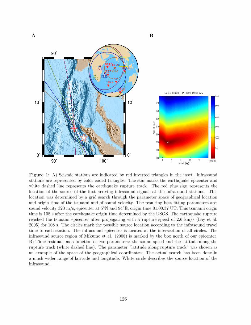
A B
Figure 1: A) Seismic stations are indicated by red inverted triangles in the inset. Infrasoundstations are represented by color coded triangles. The star marks the earthquake epicenter andwhite dashed line represents the earthquake rupture track. The red plus sign represents thelocation of the source of the first arriving infrasound signals at the infrasound stations. Thislocation was determined by a grid search through the parameter space of geographical locationand origin time of the tsunami and of sound velocity. The resulting best fitting parameters are:sound velocity 320 m/s, epicenter at 5◦N and 94◦E, origin time 01:00:37 UT. This tsunami origintime is 108 s after the earthquake origin time determined by the USGS. The earthquake rupturereached the tsunami epicenter after propagating with a rupture speed of 2.6 km/s (Lay et al.2005) for 108 s. The circles mark the possible source location according to the infrasound traveltime to each station. The infrasound epicenter is located at the intersection of all circles. Theinfrasound source region of Mikumo et al. (2008) is marked by the box north of our epicenter.B) Time residuals as a function of two parameters: the sound speed and the latitude along therupture track (white dashed line). The parameter ”latitude along rupture track” was chosen asan example of the space of the geographical coordinates. The actual search has been done ina much wider range of latitude and longitude. White circle describes the source location of theinfrasound.
126

Figure 2: Summed infrasound records of the first arriving signal from the tsunami at each of thefour infrasound arrays. The traces are filtered with an 800 s high pass filter. A) Tsunami sourceis assumed at earthquake epicenter and origin time. Traces are shifted according to a reductionvelocity of 330 m/s (meaning a wave travelling with this velocity would arrive at zero time). Theaverage infrasound speed to each station is close to 330 m/s, assuming the earthquake epicenteralso as infrasound epicenter. B) Tsunami source parameters and infrasound velocity are takenfrom the caption of Fig. 1. Infrasound first arrival times are given at the traces. The scatter ofthe wave forms in B is clearly less than in A. That means our epicenter and origin time fit theinfrasound data better than the earthquake epicenter and origin time.
127
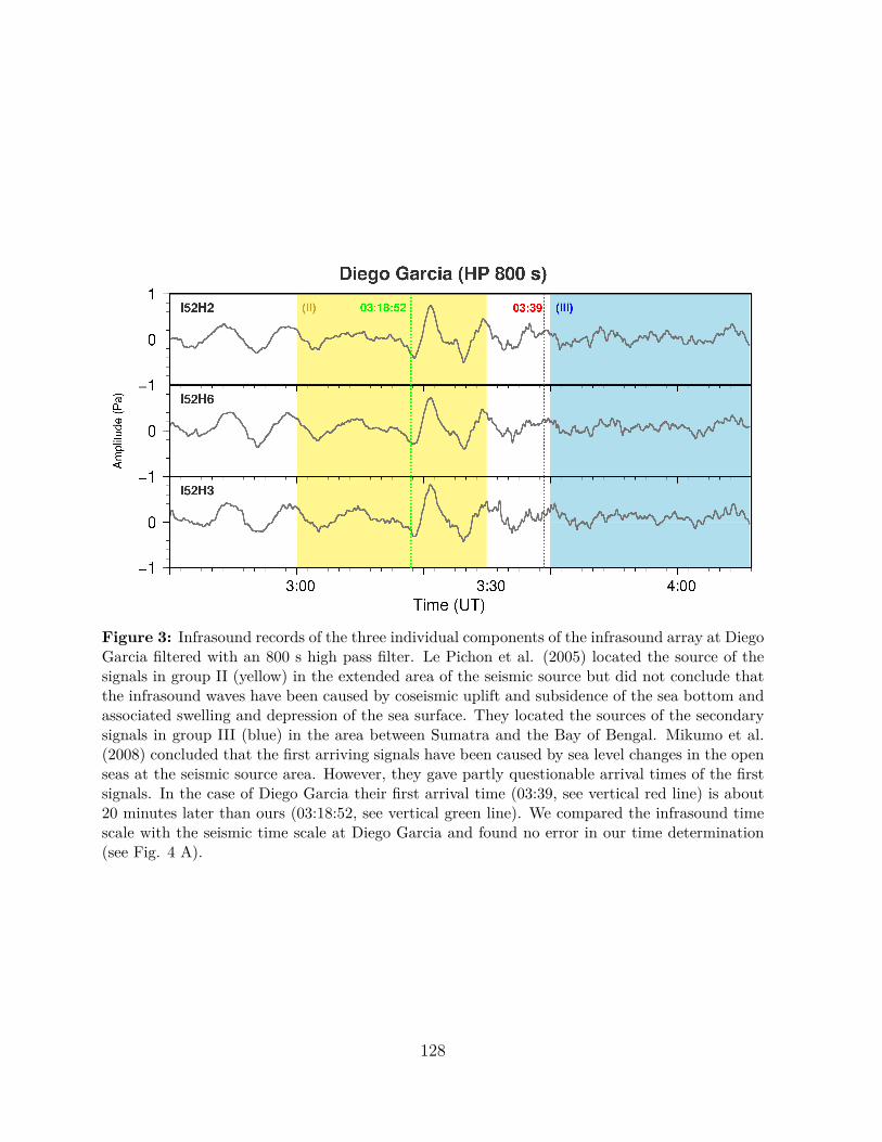
Figure 3: Infrasound records of the three individual components of the infrasound array at DiegoGarcia filtered with an 800 s high pass filter. Le Pichon et al. (2005) located the source of thesignals in group II (yellow) in the extended area of the seismic source but did not conclude thatthe infrasound waves have been caused by coseismic uplift and subsidence of the sea bottom andassociated swelling and depression of the sea surface. They located the sources of the secondarysignals in group III (blue) in the area between Sumatra and the Bay of Bengal. Mikumo et al.(2008) concluded that the first arriving signals have been caused by sea level changes in the openseas at the seismic source area. However, they gave partly questionable arrival times of the firstsignals. In the case of Diego Garcia their first arrival time (03:39, see vertical red line) is about20 minutes later than ours (03:18:52, see vertical green line). We compared the infrasound timescale with the seismic time scale at Diego Garcia and found no error in our time determination(see Fig. 4 A).
128
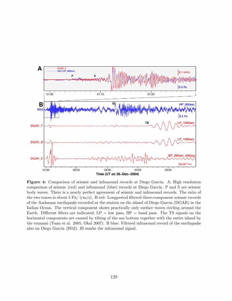
Figure 4: Comparison of seismic and infrasound records at Diego Garcia. A: High resolutioncomparison of seismic (red) and infrasound (blue) records at Diego Garcia. P and S are seismicbody waves. There is a nearly perfect agreement of seismic and infrasound records. The ratio ofthe two traces is about 5 Pa/ (cm/s). B red: Longperiod filtered three-component seismic recordsof the Andaman earthquake recorded at the station on the island of Diego Garcia (DGAR) in theIndian Ocean. The vertical component shows practically only surface waves circling around theEarth. Different filters are indicated; LP = low pass, BP = band pass. The TS signals on thehorizontal components are caused by tilting of the sea bottom together with the entire island bythe tsunami (Yuan et al. 2005, Okal 2007). B blue: Filtered infrasound record of the earthquakealso on Diego Garcia (IS52). IS marks the infrasound signal.
129
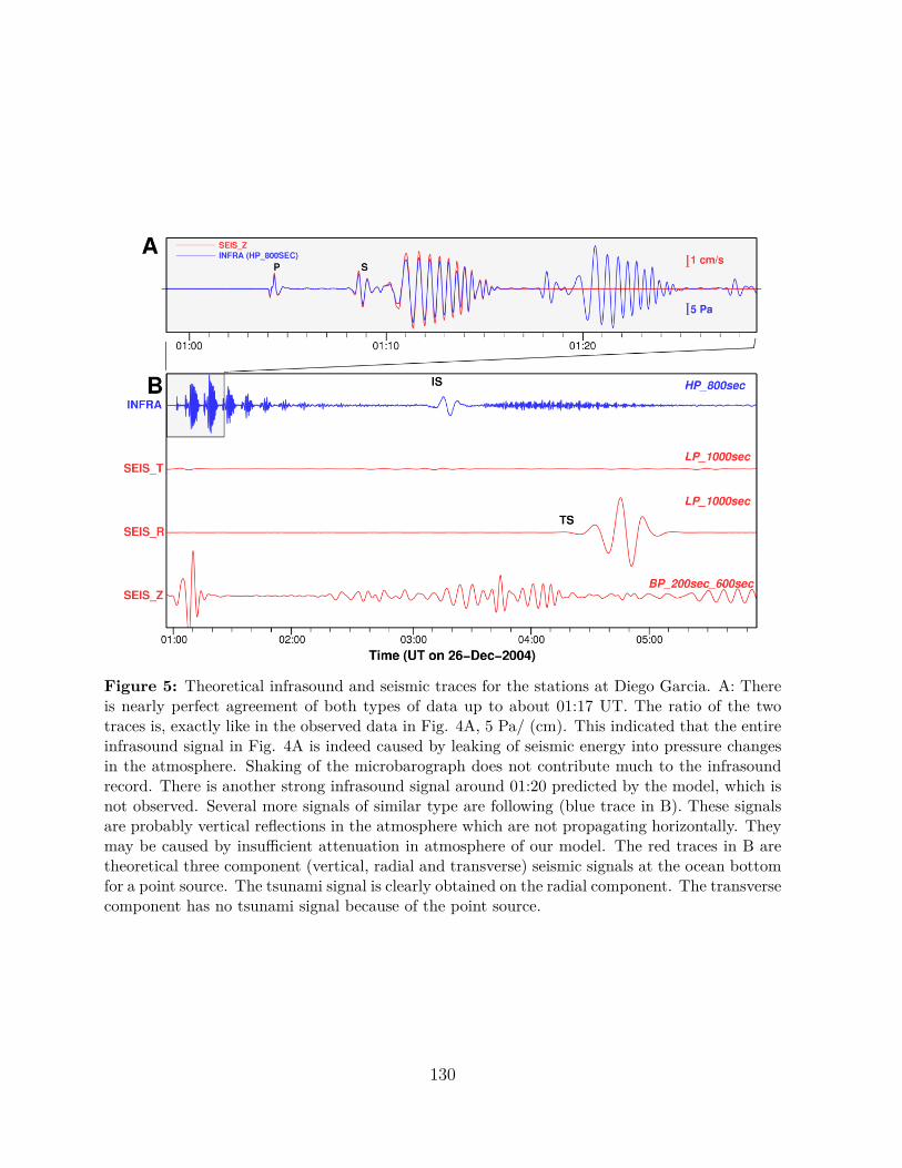
Figure 5: Theoretical infrasound and seismic traces for the stations at Diego Garcia. A: Thereis nearly perfect agreement of both types of data up to about 01:17 UT. The ratio of the twotraces is, exactly like in the observed data in Fig. 4A, 5 Pa/ (cm). This indicated that the entireinfrasound signal in Fig. 4A is indeed caused by leaking of seismic energy into pressure changesin the atmosphere. Shaking of the microbarograph does not contribute much to the infrasoundrecord. There is another strong infrasound signal around 01:20 predicted by the model, which isnot observed. Several more signals of similar type are following (blue trace in B). These signalsare probably vertical reflections in the atmosphere which are not propagating horizontally. Theymay be caused by insufficient attenuation in atmosphere of our model. The red traces in B aretheoretical three component (vertical, radial and transverse) seismic signals at the ocean bottomfor a point source. The tsunami signal is clearly obtained on the radial component. The transversecomponent has no tsunami signal because of the point source.
130
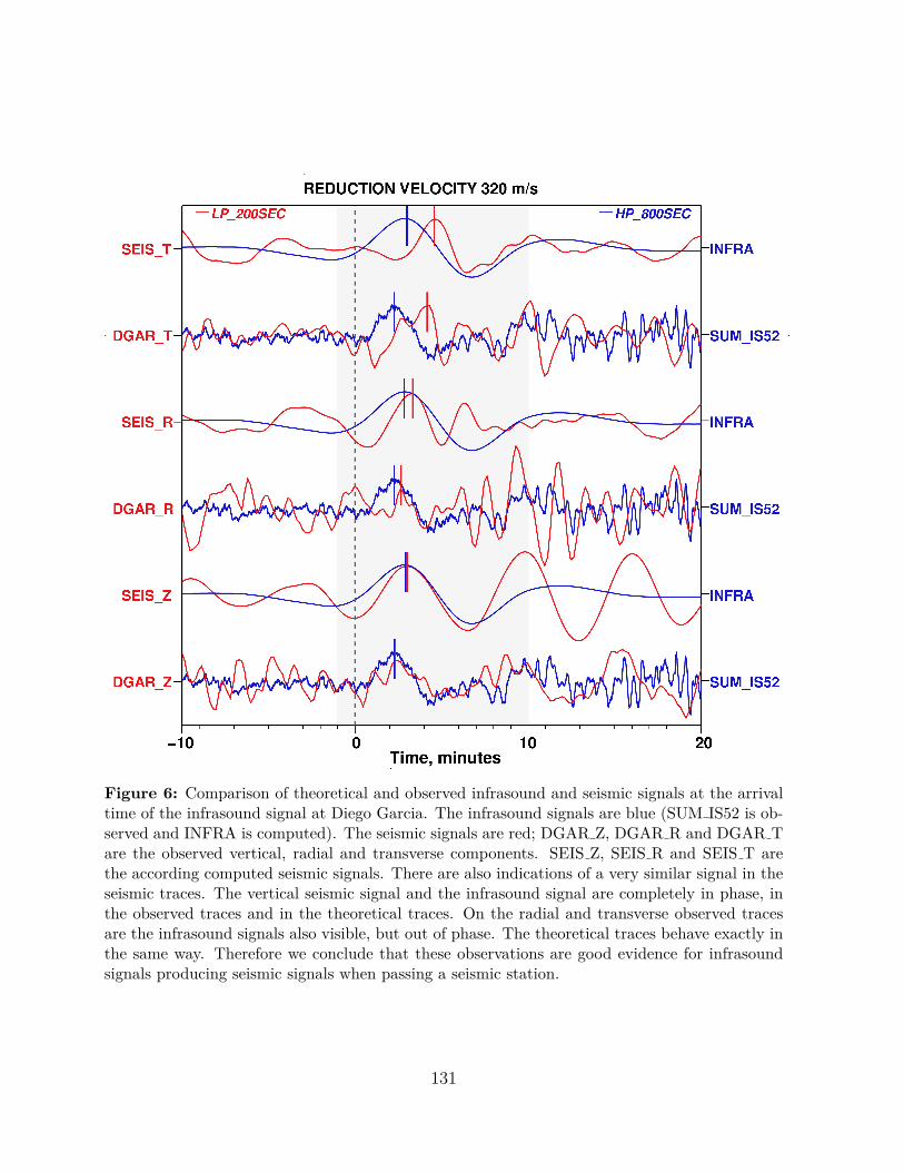
Figure 6: Comparison of theoretical and observed infrasound and seismic signals at the arrivaltime of the infrasound signal at Diego Garcia. The infrasound signals are blue (SUM IS52 is ob-served and INFRA is computed). The seismic signals are red; DGAR Z, DGAR R and DGAR Tare the observed vertical, radial and transverse components. SEIS Z, SEIS R and SEIS T arethe according computed seismic signals. There are also indications of a very similar signal in theseismic traces. The vertical seismic signal and the infrasound signal are completely in phase, inthe observed traces and in the theoretical traces. On the radial and transverse observed tracesare the infrasound signals also visible, but out of phase. The theoretical traces behave exactly inthe same way. Therefore we conclude that these observations are good evidence for infrasoundsignals producing seismic signals when passing a seismic station.
131
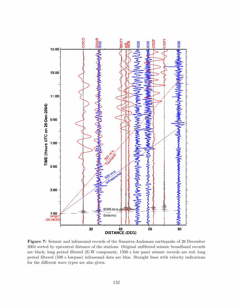
Figure 7: Seismic and infrasound records of the Sumatra-Andaman earthquake of 26 December2004 sorted by epicentral distance of the stations. Original unfiltered seismic broadband recordsare black; long period filtered (E-W component, 1500 s low pass) seismic records are red; longperiod filtered (500 s lowpass) infrasound data are blue. Straight lines with velocity indicationsfor the different wave types are also given.
132

A2) Manuscript submitted to Journal of Seismology
Locating the Tohoku-Oki 2011 Tsunami Source using Acoustic-Gravity Waves
A. Raveloson 1, R. Kind 1,2,∗, X. Yuan1, L. Ceranna3
1 GFZ Deutsches GeoForschungsZentrum, 14473 Potsdam, Germany2 also at Freie Universität, Institut für Geologische Wissenschaften, 12249 Berlin,
Germany3 Bundesanstalt für Geowissenschaften & Rohstoffe, 30655 Hannover, Germany
*Corresponding Author, email: [email protected]
AbstractThe giant Tohoku-Oki earthquake of 11 March 2011 offshore Japan did not only generate
tsunami waves in the ocean but also infrasound (or acoustic-gravity) waves in the atmo-
sphere. We identified ultra longperiod signals in the recordings of infrasound stations in
north-east Asia, the north-west Pacific and Alaska. Their source was found to be close to
the earthquake epicenter. Therefore, we conclude that in general infrasound observations
after a large offshore earthquake are evidence, that the surface and the floor of the sea
have been significantly displaced by the earthquake and that a tsunami must be expected.
Since infrasound is travelling faster than the tsunami, this information may be used for
tsunami early warnings.
IntroductionThe magnitude 9.0 Tohoku-Oki earthquake on 11 March 2011 in Japan [e.g. Simons et
al. 2011] caused one of the largest and most devastating tsunamis ever observed on Earth.
The tsunami early warning system of the Japan Meteorological Agency saved many lives
by issuing a timely warning. However, the tsunami still caused thousands of casualties
because its size was not properly predicted. The first step in a tsunami warning system is
the fast determination of the location and size of the offshore earthquake, which is used to
133
model the possible tsunami at the shorelines. However, at this point it is not even certain
if a tsunami has been generated at all. The first direct observation of the tsunami may
be obtained from ocean bottom pressure gauges in the vicinity of the source, if they are
available. The next direct tsunami observations usually come from tide gauge stations at
the shorelines. However, at this point the tsunami has already reached the shores and the
warning time tends to zero.
Already Bolt (1964) observed acoustic-gravity waves from the great 1964 Alaska earth-
quake and he suggested using them for tsunami warnings. Atmospheric pressure waves
travel with a speed of about 300m/sec whereas tsunami waves travel with 200m/sec in
the deep sea and much slower in shallower coastal regions. This difference may result in a
very useful tsunami warning time. Mikumo et al. (2008) identified acoustic-gravity waves
with periods of about 500sec caused by the great 2004 Sumatra-Andaman earthquake and
used them to estimate the dislocation of the sea level in the source region. Raveloson et
al. (2011) also used long period acoustic-gravity waves of the same event to improve the
location of the tsunami source.
Data and MethodWe searched through the data of the infrasound arrays of the International Monitoring
System in Vienna (IMS, http://www.ctbto.org/ ) for signals of the Tohoku-Oki tsunami.
The locations of the infrasound arrays used in our study are shown in Fig.1. Each of these
arrays consists of 4-8 microbarographs located within several kilometers. Because of the
small aperture of the arrays and our interest in the longest periods ( 500sec), we summed
all the individual components of each array into one summation trace without applying
any time shifts. That means we did not used typical array properties (like measurements
of slowness and backazimuth of an incoming sound wave), but treated each array as single
134
station and used the individual array stations only to improve the signal-to-noise ratio.
Clear signals were found thousands of kilometers away from the source in continental Asia
and Alaska. These signals are displayed in Fig.2a. Picked arrival times of the infrasound
signals are marked in Fig.2a at the individual traces. We located the tsunami source by
a simple grid search method over the coordinates of the infrasound source location and
the sound speed. The origin time of the earthquake was used as the origin time of the
infrasound wave. The resulting source location is displayed in Fig.2b and the infrasound
speed, which leads to the closest location of the circle intersections, is 290m/sec, using only
the stations in Asia. Delays of the infrasound origin time relative to the earthquake origin
time by up to 100s changed the location of the infrasound source by less than 50km.
The station in Alaska (IS53, see Fig.1) is the station with the largest outlier of its inter-
section points and was ignored in the source location. The best sound speed would be
356m/sec for this station. The velocities of infrasound are generally near 300m/sec with
variations of ś50m/sec due to wind speed (Arrowsmith et al. 2010). Our observed sound
speeds of 290 and 356m/sec are within this window. The wind in Japan was blowing from
the west at the time of the earthquake and its speed on the ground was near 30km/h (ref).
The wind speed in larger altitudes is not known to us, but could be higher than on the
ground. A strong wind component (about 100km/h) blowing in the opposite direction for
the Asian (backazimuth north-west) and Alaskan (backazimuth north-east) stations could
be responsible for the different travel times in the different directions. Fig.3 shows the
infrasound records of the stations IS39 and IS44 (stations in black in Fig.1) in comparison
with the station IS53 in Alaska. A very weak signal may be detected at station IS44, which
has a similar backazimuth like the Alaskan station. No signal is detectable above the noise
level at station IS39 in the western Pacific, which has a backazimuth nearly opposite to
the Alaskan station. This might be an effect of source directivity.
135
Results and ConclusionsFig.2b shows the locations of the earthquake epicenter according to the USGS, our location
of the infrasound source and the distribution of vertical displacements of the sea bottom
measured at ocean bottom GPS stations. The largest GPS displacement of the sea bottom
and the two epicenters are located within about 100km of each other. It should be kept in
mind that all infrasound stations (except one) used for the source location are thousands
of kilometers away from the source. Data from a larger number of better distributed and
closer infrasound stations would certainly increase the accuracy of the location of the infra-
sound source. Our most important result is therefore, that the Tohoku-Oki earthquake has
generated dislocations of the sea surface in the epicentral region of the earthquake, which
acted as source of ultra longperiod infrasound signals. From this we conclude that the in-
frasound source region is also the source region of the tsunami and the region with largest
vertical displacements of the sea bottom. Modeling of the observed infrasound signals may
contribute additional parameters to the earthquake source characteristics (Mikumo et al.
2008).
A second important aspect of our study is that real-time processing of infrasound obser-
vations may improve tsunami modeling for early warning purposes. Assuming an average
water depth of 1000m, the speed of the tsunami is about three times less than the speed
of infrasound. This means a tsunami needs about 15 minutes to reach a coast 100km away
from the epicenter. The infrasound signal of the tsunami already indicates 5 minutes after
the origin time that a tsunami is definitely coming. From the size and the regional distri-
bution of the infrasound signals a better modeling of the tsunami arriving at the shores
may be obtained.
136
AcknowledgementWe wish to thank James Mechie for reading the manuscript.
ReferencesArrowsmith, S.J., Johnson, J.B. and Drop, D.P., 2010, The Seismoacoustic Wavefield: A
new Paradigm in Studying Geophysical Phenomena, Review of Geophysics, 48, RG4003,
DOI: 10.1029/2010RG000335.
Bolt, B.A., 1964, Seismic air waves from the great 1964 Alaskan earthquake, Nature, 202,
1095- 1096, doi:10.1038/2021095a0.
Mikumo, T., Shibutani, T., Le Pichon, A., Garces, M., Fee, D., Tsuyuki, T., Watada, S.
and Morii, W., 2008, Low-frequency acoustic-gravity waves from coseismic vertical defor-
mation associated with the 2004 Sumatra-Andaman earthquake (Mw = 9.2), J. Geophys.
Res., 113.
Raveloson, A., Wang, R., Kind, R., Ceranna, L. and Yuan, X., 2011, Seismic and Infra-
sound Signals from the 2004 Indian Ocean Tsunami, Geophys. J. Int., submitted.
Sato, M., Ishikawa, T., Ujihara, N. et al., 2011, Displacement above the Hypocenter of the
2011 Tohoku-Oki Earthquake, Science, 332, 1395-1395, DOI:10.1126/science.120740.
Simons, M., Minson, S.E., Sladen, A. et al., 2011, The 2011 Magnitude 9.0 Tohoku-Oki
Earthquake: Mosaicking the Megathrust from Seconds to Centuries, Science, 332, 1421-
1425.
Figures
137
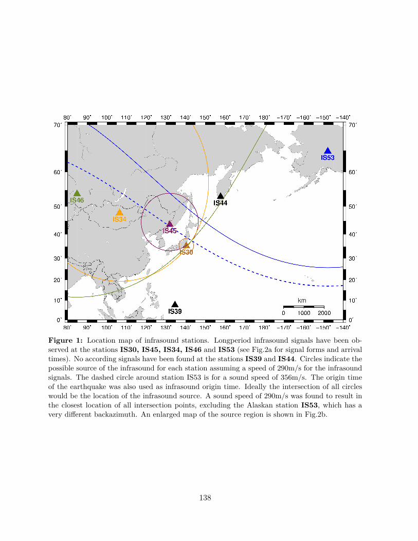
Figure 1: Location map of infrasound stations. Longperiod infrasound signals have been ob-served at the stations IS30, IS45, IS34, IS46 and IS53 (see Fig.2a for signal forms and arrivaltimes). No according signals have been found at the stations IS39 and IS44. Circles indicate thepossible source of the infrasound for each station assuming a speed of 290m/s for the infrasoundsignals. The dashed circle around station IS53 is for a sound speed of 356m/s. The origin timeof the earthquake was also used as infrasound origin time. Ideally the intersection of all circleswould be the location of the infrasound source. A sound speed of 290m/s was found to result inthe closest location of all intersection points, excluding the Alaskan station IS53, which has avery different backazimuth. An enlarged map of the source region is shown in Fig.2b.
138
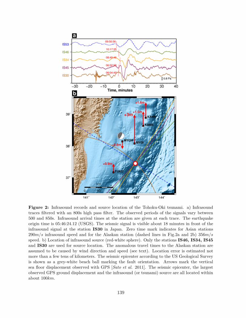
Figure 2: Infrasound records and source location of the Tohoku-Oki tsunami. a) Infrasoundtraces filtered with an 800s high pass filter. The observed periods of the signals vary between500 and 850s. Infrasound arrival times at the station are given at each trace. The earthquakeorigin time is 05:46:24.12 (USGS). The seismic signal is visible about 18 minutes in front of theinfrasound signal at the station IS30 in Japan. Zero time mark indicates for Asian stations290m/s infrasound speed and for the Alaskan station (dashed lines in Fig.2a and 2b) 356m/sspeed. b) Location of infrasound source (red-white sphere). Only the stations IS46, IS34, IS45and IS30 are used for source location. The anomalous travel times to the Alaskan station areassumed to be caused by wind direction and speed (see text). Location error is estimated notmore than a few tens of kilometers. The seismic epicenter according to the US Geological Surveyis shown as a grey-white beach ball marking the fault orientation. Arrows mark the verticalsea floor displacement observed with GPS [Sato et al. 2011]. The seismic epicenter, the largestobserved GPS ground displacement and the infrasound (or tsunami) source are all located withinabout 100km.
139
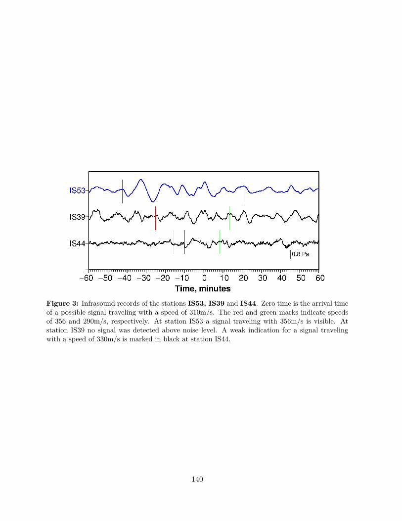
Figure 3: Infrasound records of the stations IS53, IS39 and IS44. Zero time is the arrival timeof a possible signal traveling with a speed of 310m/s. The red and green marks indicate speedsof 356 and 290m/s, respectively. At station IS53 a signal traveling with 356m/s is visible. Atstation IS39 no signal was detected above noise level. A weak indication for a signal travelingwith a speed of 330m/s is marked in black at station IS44.
140