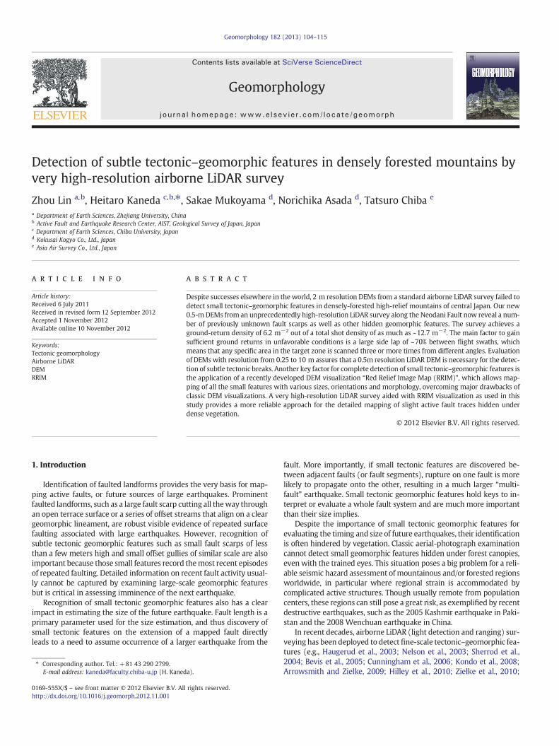
Geomorphology 182 (2013) 104–115

Contents lists available at SciVerse ScienceDirect

Geomorphology

j ourna l homepage: www.e lsev ie r .com/ locate /geomorph

Detection of subtle tectonic–geomorphic features in densely forested mountains byvery high-resolution airborne LiDAR survey

Zhou Lin a,b, Heitaro Kaneda c,b,⁎, Sakae Mukoyama d, Norichika Asada d, Tatsuro Chiba e

a Department of Earth Sciences, Zhejiang University, Chinab Active Fault and Earthquake Research Center, AIST, Geological Survey of Japan, Japanc Department of Earth Sciences, Chiba University, Japand Kokusai Kogyo Co., Ltd., Japane Asia Air Survey Co., Ltd., Japan

⁎ Corresponding author. Tel.: +81 43 290 2799.E-mail address: kaneda@faculty.chiba-u.jp (H. Kaned

0169-555X/$ – see front matter © 2012 Elsevier B.V. Alhttp://dx.doi.org/10.1016/j.geomorph.2012.11.001

a b s t r a c t

a r t i c l e i n f o

Article history:Received 6 July 2011Received in revised form 12 September 2012Accepted 1 November 2012Available online 10 November 2012

Keywords:Tectonic geomorphologyAirborne LiDARDEMRRIM

Despite successes elsewhere in the world, 2 m resolution DEMs from a standard airborne LiDAR survey failed todetect small tectonic–geomorphic features in densely-forested high-relief mountains of central Japan. Our new0.5-m DEMs from an unprecedentedly high-resolution LiDAR survey along the Neodani Fault now reveal a num-ber of previously unknown fault scarps as well as other hidden geomorphic features. The survey achieves aground-return density of 6.2 m−2 out of a total shot density of as much as ~12.7 m−2. The main factor to gainsufficient ground returns in unfavorable conditions is a large side lap of ~70% between flight swaths, whichmeans that any specific area in the target zone is scanned three or more times from different angles. Evaluationof DEMswith resolution from 0.25 to 10 m assures that a 0.5m resolution LiDAR DEM is necessary for the detec-tion of subtle tectonic breaks. Another key factor for complete detection of small tectonic–geomorphic features isthe application of a recently developed DEM visualization “Red Relief Image Map (RRIM)”, which allows map-ping of all the small features with various sizes, orientations and morphology, overcoming major drawbacks ofclassic DEM visualizations. A very high-resolution LiDAR survey aided with RRIM visualization as used in thisstudy provides a more reliable approach for the detailed mapping of slight active fault traces hidden underdense vegetation.

© 2012 Elsevier B.V. All rights reserved.

1. Introduction

Identification of faulted landforms provides the very basis for map-ping active faults, or future sources of large earthquakes. Prominentfaulted landforms, such as a large fault scarp cutting all theway throughan open terrace surface or a series of offset streams that align on a cleargeomorphic lineament, are robust visible evidence of repeated surfacefaulting associated with large earthquakes. However, recognition ofsubtle tectonic geomorphic features such as small fault scarps of lessthan a few meters high and small offset gullies of similar scale are alsoimportant because those small features record themost recent episodesof repeated faulting. Detailed information on recent fault activity usual-ly cannot be captured by examining large-scale geomorphic featuresbut is critical in assessing imminence of the next earthquake.

Recognition of small tectonic geomorphic features also has a clearimpact in estimating the size of the future earthquake. Fault length is aprimary parameter used for the size estimation, and thus discovery ofsmall tectonic features on the extension of a mapped fault directlyleads to a need to assume occurrence of a larger earthquake from the

a).

l rights reserved.

fault. More importantly, if small tectonic features are discovered be-tween adjacent faults (or fault segments), rupture on one fault is morelikely to propagate onto the other, resulting in a much larger “multi-fault” earthquake. Small tectonic geomorphic features hold keys to in-terpret or evaluate a whole fault system and are much more importantthan their size implies.

Despite the importance of small tectonic geomorphic features forevaluating the timing and size of future earthquakes, their identificationis often hindered by vegetation. Classic aerial-photograph examinationcannot detect small geomorphic features hidden under forest canopies,even with the trained eyes. This situation poses a big problem for a reli-able seismic hazard assessment of mountainous and/or forested regionsworldwide, in particular where regional strain is accommodated bycomplicated active structures. Though usually remote from populationcenters, these regions can still pose a great risk, as exemplified by recentdestructive earthquakes, such as the 2005 Kashmir earthquake in Paki-stan and the 2008 Wenchuan earthquake in China.

In recent decades, airborne LiDAR (light detection and ranging) sur-veying has been deployed to detect fine-scale tectonic–geomorphic fea-tures (e.g., Haugerud et al., 2003; Nelson et al., 2003; Sherrod et al.,2004; Bevis et al., 2005; Cunningham et al., 2006; Kondo et al., 2008;Arrowsmith and Zielke, 2009; Hilley et al., 2010; Zielke et al., 2010;

105Z. Lin et al. / Geomorphology 182 (2013) 104–115

Oskin et al., 2012), and to quantitatively explore characteristics of tec-tonic geomorphology (e.g., Hilley and Arrowsmith, 2008; Wechsler etal., 2009; Hilley et al., 2010; Zielke et al., 2010). One of the most attrac-tive benefits of airborne LiDAR is its ability to see through the “bareearth” under vegetation because the ground emits a laser pulse thatcan be separated from canopy returns through filtering processes. Inthe U.S. Pacific NW and Europe, studies have successfully delineatedearthquake surface ruptures under vegetation using 2-m LiDAR DEMs(digital elevation models) (Harding and Berghoff, 2000; Haugerud etal., 2003; Sherrod et al., 2004; Cunningham et al., 2006). However, re-cent LiDAR studies on the northern San Andreas Fault and centralJapanese mountains also reported that some small tectonic breakscould not be identified with this resolution (Zachariasen, 2008; Lin etal., 2009; National Institute of Advanced Industrial Science andTechnology, AIST, 2009). Especially in the case of high-relief Japanesemountains, we failed to find any youthful tectonic features by the 2-mDEMs from standard LiDAR surveys (National Institute of AdvancedIndustrial Science and Technology, AIST, 2009). Dense vegetation andtopographic complexity likely increased the number of off-terrainlaser hits, thereby reducing the number of ground laser strikes. The re-sults showed that the ground data with low density failed to capturesubtle geomorphic features. There is an urgent need to examine and ex-pand the capabilities of LiDAR DEMs on their topographic expression.

One simple approach to address this issue is to increase spatial reso-lution of LiDAR ground return data. The development of recent LiDARtechnique allows higher pulse-shot frequency. Lower flight altitude andmore dense flight passes also aid more LiDAR pulses to transfer throughthe canopy and to reach the ground. Based on the enough data density,much finer resolution of LiDAR DEMs of tens of centimeters now canbe constructed.

Another important, but often overlooked approach for more com-plete small-feature detection is to improve visualization of DEMs. High-resolution LiDAR DEMs are generally examined on a shaded relief mapand/or a slope map. The former is widely used because it resembleswhat we see in the real world, but has a big disadvantage in that the ap-pearance and impression of the image completely change depending onthe direction of incident illumination. The latter is illumination-independent, but is quite different from our vision and cannot distin-guish convexity and concavity. Fine-scale tectonic features with varyingorientations will be obscured as a result of the limitations.

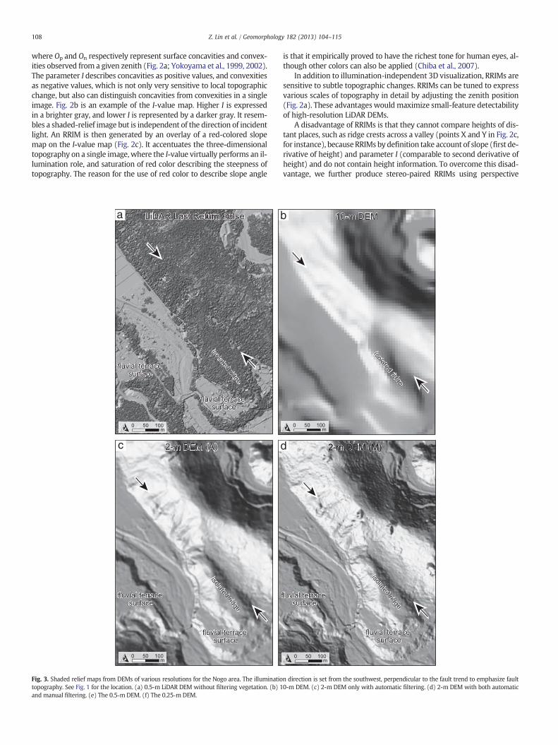
The purpose of this study is to explore effective LiDAR surveys andDEMvisualizationmethods formapping small tectonic geomorphic fea-tures in densely vegetated high-relief mountains. The study area is thenorthern part of the Neodani Fault, an active strike–slip fault in centralJapanese mountains, where previous 2-m DEMs from standard LiDARsurvey failed to detect small geomorphic features (National Instituteof Advanced Industrial Science and Technology, AIST, 2009). Weconducted an unprecedentedly high-resolution LiDAR survey in thesame area, and the new LiDAR DEMs were compared with the existing2-m LiDAR DEMs as well as topographic-map-based 10-m DEMs to ex-amine if there was increased topographic expression of subtle features.In order to further enhance detectability of subtle topographic features,we applied a recently developed elaborate visualization “Red ReliefImage Map (RRIM)” (Chiba et al., 2008) to the new LiDAR DEMs. Appli-cation of RRIMs to the high-resolution LiDAR DEMs allows fine expres-sion of topography without shading, and serves as a very effective wayfor the detailed depiction of the slight tectonic–geomorphic features be-neath dense vegetation. Though largely based on qualitative analyses,we suggest that a combination of a high-resolution LiDAR survey andRRIM visualization is effective for a complete and detailed mapping ofslight active fault traces in densely vegetated high-relief mountains.

2. Study area

TheNeodani Fault is anNW–SE striking active left-lateral fault in cen-tral Japanese mountains. It is one of the main faults that ruptured in the

devastating 1891 Mw 7.5 Nobi earthquake (Fig. 1; Matsuda, 1974). Asmultiple faults were involved in the 1891 earthquake, past behavioralpatterns of those faults has received particular interest (e.g., Okada andMatsuda, 1992; Awata et al., 1999; Yoshioka et al., 2002; Kaneda andOkada, 2008). However, because of dense forest covers and rugged to-pography, the location of the northernmost part of the Neodani Faulthas not yet been well defined by aerial photograph interpretation or byfield investigation. In this study, we selected the northern part of theNeodani Fault as a target area of the new airborne LiDAR survey(Fig. 1). The area has the steepest topography along the fault zone,with altitudes of 156.2 to 1540.9 m, and average slope angle around35°. The main rock type is Paleozoic–Mesozoic sedimentary rocks withpenetration of Miocene granite. Most hillslopes are thickly covered bydeciduous broad-leaved trees (mainly Japanese oaks and beeches), ever-green coniferous trees (mainly Japanese cedars and cypresses), under-growth of bamboo grasses (Kumazawa) and other thorny bushes. Theclimate of the study area is warm and temperate with a mean annualtemperature of ca. 8–16 °C. The average annual precipitation is about2500 mm (Japan Meteorological Agency, 1971).

3. Data and methods

3.1. Very high-resolution LiDAR survey

A very high-resolution airborne LiDAR survey was conducted alongthe northern part of the Neodani Fault (Fig. 1) during the leaf-off seasonof January 2008. The target area is ~16 km long and ~1.25 km wide. ACessna 208 with a Leica ALS 50 LiDAR instrument was flown at an alti-tude of ~1250 m, which is a lower limit in high-relief mountain areas,scanning the topography with a pulse-shot frequency of 50–60 kHz,scan angle of ±~10°, and a swath width of ~430 m. The LiDAR surveywas carried out by Kokusai Kogyo Co., Ltd., Japan.

The key factor for the achievement of a very high shot density alongthe fault is an exceptionally large number of flight passes in the targetzone. We set up as many as 13 passes targeting the 1.25-km-wide zone,as compared to five passes targeting the zone of similar width in the re-cent LiDAR survey project (“B4 project”) along the southern San AndreasFault (e.g., Arrowsmith and Zielke, 2009; Zielke et al., 2010). This is equiv-alent to a side lap (overlap of swaths) of ~70%,whichmeans that any spe-cific area in the target zone is scanned three or more times from differentangles. This sampling approach is more efficient than simply increasingthe pulse shot frequency or decreasingflight height and proved particularuseful for gaining higher-density ground returns in steep topography. Theresultant average shot density of the laser points before filtering is asmuch as ~12.7 m−2, ranging from 6.7 to 24.6 m−2. This not only over-whelms that of the previous 2003–2004 LiDAR survey (~1.2 m−2) thatwill be described later, but is evenmuch higher than that of the more re-cent B4 project along the San Andreas (~3.6 m−2; Arrowsmith andZielke, 2009). The acquired elevation data has a horizontal accuracy of0.320 m, a vertical accuracy of 0.085 m, and an absolute RMS accuracybetter than 0.15 m.

Automatic filtering was performed to eliminate vegetation and man-made structures using an adaptive filter that evaluates changes in slopesand elevation along the scan line. Thefiltering is based on the assumptionthat natural terrain variations are gradual, rather than abrupt. In contrast,the boundary between ground and non-ground points should exhibit anabrupt change in elevation and slope. The joint use of slopes, elevationdifferences, and local elevations can help to filter non-ground pointsmore accurately. In addition, we closely checked the automatic filteringdata and manually eliminated or restored the error points to constructmore realistic ground return data. After the filtering, the average shotdensity of ground points is still around 6.2 m−2, indicating one out oftwo shots reached the ground on average. Based on the ground pointdata, 0.5-m DEMs were generated. Higher resolution DEMs (0.25 m)were also generated for portions of the fault where average shot densityis larger than 12.0 m−2.

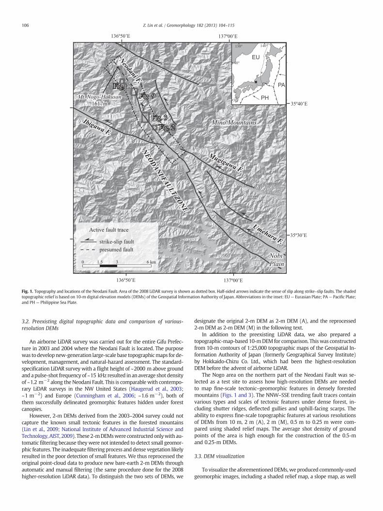
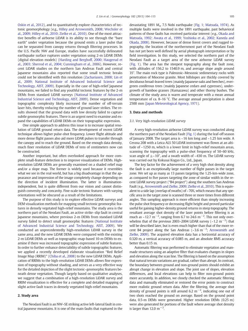
Fig. 1. Topography and locations of the Neodani Fault. Area of the 2008 LiDAR survey is shown as dotted box. Half-sided arrows indicate the sense of slip along strike–slip faults. The shadedtopographic relief is based on 10-m digital elevation models (DEMs) of the Geospatial Information Authority of Japan. Abbreviations in the inset: EU— Eurasian Plate; PA— Pacific Plate;and PH — Philippine Sea Plate.

106 Z. Lin et al. / Geomorphology 182 (2013) 104–115

3.2. Preexisting digital topographic data and comparison of various-resolution DEMs

An airborne LiDAR survey was carried out for the entire Gifu Prefec-ture in 2003 and 2004 where the Neodani Fault is located. The purposewas todevelopnew-generation large-scale base topographicmaps for de-velopment, management, and natural-hazard assessment. The standard-specification LiDAR survey with a flight height of ~2000 m above groundand apulse-shot frequency of ~15 kHz resulted in an average shot densityof ~1.2 m−2 along the Neodani Fault. This is comparable with contempo-rary LiDAR surveys in the NW United States (Haugerud et al., 2003;~1 m−2) and Europe (Cunningham et al., 2006; ~1.6 m−2), both ofthem successfully delineated geomorphic features hidden under forestcanopies.

However, 2-m DEMs derived from the 2003–2004 survey could notcapture the known small tectonic features in the forested mountains(Lin et al., 2009; National Institute of Advanced Industrial Science andTechnology, AIST, 2009). These 2-mDEMswere constructedonlywith au-tomatic filtering because theywere not intended to detect small geomor-phic features. The inadequatefiltering process and dense vegetation likelyresulted in the poor detection of small features. We thus reprocessed theoriginal point-cloud data to produce new bare-earth 2-m DEMs throughautomatic and manual filtering (the same procedure done for the 2008higher-resolution LiDAR data). To distinguish the two sets of DEMs, we

designate the original 2-m DEM as 2-m DEM (A), and the reprocessed2-m DEM as 2-m DEM (M) in the following text.

In addition to the preexisting LiDAR data, we also prepared atopographic-map-based 10-mDEM for comparison. Thiswas constructedfrom 10-m contours of 1:25,000 topographic maps of the Geospatial In-formation Authority of Japan (formerly Geographical Survey Institute)by Hokkaido-Chizu Co. Ltd., which had been the highest-resolutionDEM before the advent of airborne LiDAR.

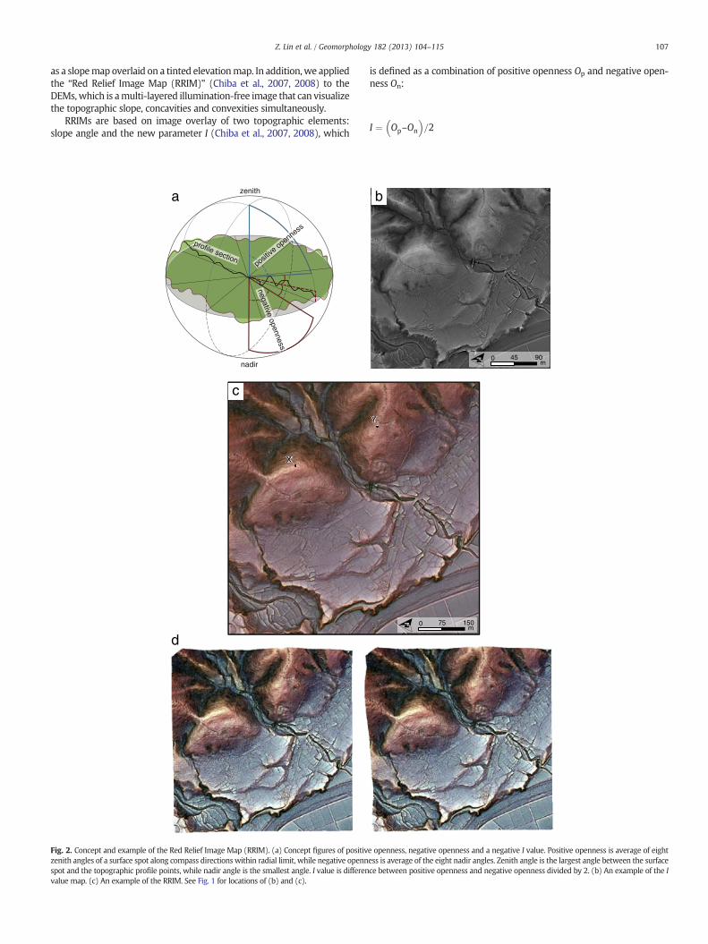
The Nogo area on the northern part of the Neodani Fault was se-lected as a test site to assess how high-resolution DEMs are neededto map fine-scale tectonic–geomorphic features in densely forestedmountains (Figs. 1 and 3). The NNW–SSE trending fault traces containvarious types and scales of tectonic features under dense forest, in-cluding shutter ridges, deflected gullies and uphill-facing scarps. Theability to express fine-scale topographic features at various resolutionsof DEMs from 10 m, 2 m (A), 2 m (M), 0.5 m to 0.25 m were com-pared using shaded relief maps. The average shot density of groundpoints of the area is high enough for the construction of the 0.5-mand 0.25-m DEMs.

3.3. DEM visualization

To visualize the aforementionedDEMs,we produced commonly-usedgeomorphic images, including a shaded relief map, a slope map, as well

107Z. Lin et al. / Geomorphology 182 (2013) 104–115

as a slopemap overlaid on a tinted elevationmap. In addition,we appliedthe “Red Relief Image Map (RRIM)” (Chiba et al., 2007, 2008) to theDEMs,which is amulti-layered illumination-free image that can visualizethe topographic slope, concavities and convexities simultaneously.

RRIMs are based on image overlay of two topographic elements:slope angle and the new parameter I (Chiba et al., 2007, 2008), which

nadir

zenith

profile sectionposit

ive openness

negative openness

c

XX

d

a

Fig. 2. Concept and example of the Red Relief Image Map (RRIM). (a) Concept figures of positivzenith angles of a surface spot along compass directions within radial limit, while negative opennspot and the topographic profile points, while nadir angle is the smallest angle. I value is differenvalue map. (c) An example of the RRIM. See Fig. 1 for locations of (b) and (c).

is defined as a combination of positive openness Op and negative open-ness On:

I ¼ Op–On

� �=2

YY

15075m

0

9045m

0

b

e openness, negative openness and a negative I value. Positive openness is average of eightess is average of the eight nadir angles. Zenith angle is the largest angle between the surfacece between positive openness and negative openness divided by 2. (b) An example of the I

108 Z. Lin et al. / Geomorphology 182 (2013) 104–115

where Op and On respectively represent surface concavities and convex-ities observed from a given zenith (Fig. 2a; Yokoyama et al., 1999, 2002).The parameter I describes concavities as positive values, and convexitiesas negative values, which is not only very sensitive to local topographicchange, but also can distinguish concavities from convexities in a singleimage. Fig. 2b is an example of the I-value map. Higher I is expressedin a brighter gray, and lower I is represented by a darker gray. It resem-bles a shaded-relief image but is independent of the direction of incidentlight. An RRIM is then generated by an overlay of a red-colored slopemap on the I-value map (Fig. 2c). It accentuates the three-dimensionaltopography on a single image, where the I-value virtually performs an il-lumination role, and saturation of red color describing the steepness oftopography. The reason for the use of red color to describe slope angle

a b

c d

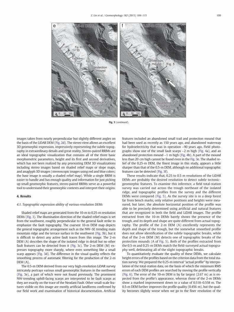
Fig. 3. Shaded relief maps from DEMs of various resolutions for the Nogo area. The illuminatiotopography. See Fig. 1 for the location. (a) 0.5-m LiDAR DEM without filtering vegetation. (b) 1and manual filtering. (e) The 0.5-m DEM. (f) The 0.25-m DEM.

is that it empirically proved to have the richest tone for human eyes, al-though other colors can also be applied (Chiba et al., 2007).

In addition to illumination-independent 3D visualization, RRIMs aresensitive to subtle topographic changes. RRIMs can be tuned to expressvarious scales of topography in detail by adjusting the zenith position(Fig. 2a). These advantages would maximize small-feature detectabilityof high-resolution LiDAR DEMs.

A disadvantage of RRIMs is that they cannot compare heights of dis-tant places, such as ridge crests across a valley (points X and Y in Fig. 2c,for instance), becauseRRIMs by definition take account of slope (first de-rivative of height) and parameter I (comparable to second derivative ofheight) and do not contain height information. To overcome this disad-vantage, we further produce stereo-paired RRIMs using perspective

n direction is set from the southwest, perpendicular to the fault trend to emphasize fault0-m DEM. (c) 2-m DEM only with automatic filtering. (d) 2-m DEM with both automatic

e f

Fig. 3 (continued).

109Z. Lin et al. / Geomorphology 182 (2013) 104–115

images taken from nearly perpendicular but slightly different angles onthe basis of the LiDARDEM (Fig. 2d). The stereo view allows an excellent3D geomorphic expression, impressively representing the subtle topog-raphy in extraordinary details and great reality. Stereo-paired RRIMs arean ideal topographic visualization that contains all of the three basicmorphometric parameters, height and its first and second derivatives,which has not been realized by any preexisting DEM 3D visualizationsincluding stereo images based on shaded relief maps or slope maps,and anaglyph 3D images (stereoscopic images using red and blue colors;the base image is usually a shaded relief map). While a single RRIM iseasier to handle and has enough quality and information for just pickingup small geomorphic features, stereo-paired RRIMs serve as a powerfultool to understand their geomorphic contexts and interpret their origins.

4. Results

4.1. Topographic expression ability of various-resolution DEMs

Shaded relief maps are generated from the 10-m to 0.25-m resolutionDEMs (Fig. 3). The illumination direction of the shaded relief maps is setfrom the southwest, roughly perpendicular to the general fault strike toemphasize the fault topography. The coarsest 10-m DEM map depictsthe general topographic arrangement such as the NW–SE trending mainmountain ridge and the terrace surface in the southwest (Fig. 3b), but itis difficult to detect any active fault traces from this image. The 2-mDEM (A) describes the shape of the isolated ridge in detail but no otherfault features can be detected from it (Fig. 3c). The 2-m DEM (M) ex-presses topography more sharply, where even something like a smallscarp appears (Fig. 3d). The difference in the visual quality reflects thesmoothing process of automatic filtering for the production of the 2-mDEM (A).

The 0.5-m DEM derived from our very high-resolution LiDAR surveyintricately portrays various small geomorphic features in the northwest(Fig. 3e), a part of which were not found previously. The prominentNW-trending uphill-facing scarps are interpreted to be fault scarps asthey are exactly on the trace of the Neodani Fault. Other small-scale fea-tures visible on this image are mostly artificial landforms confirmed byour field work and examination of historical documentation. Artificial

features included an abandoned small trail and protection mound thathad been used as recently as 150 years ago, and abandoned waterwayfor hydroelectricity that was in operation ~90 years ago. Field photo-graphs show one of the small fault scarps ~2 m high (Fig. 4a), and anabandoned protection mound ~1 m high (Fig. 4b). A part of the moundless than 20 cm high cannot be found even in the Fig. 3e. The shaded re-lief of the 0.25-m DEM, the finest image in this study, appears a littlesharper than that of the 0.5-m DEM, although no additional topographicfeatures can be detected (Fig. 3f).

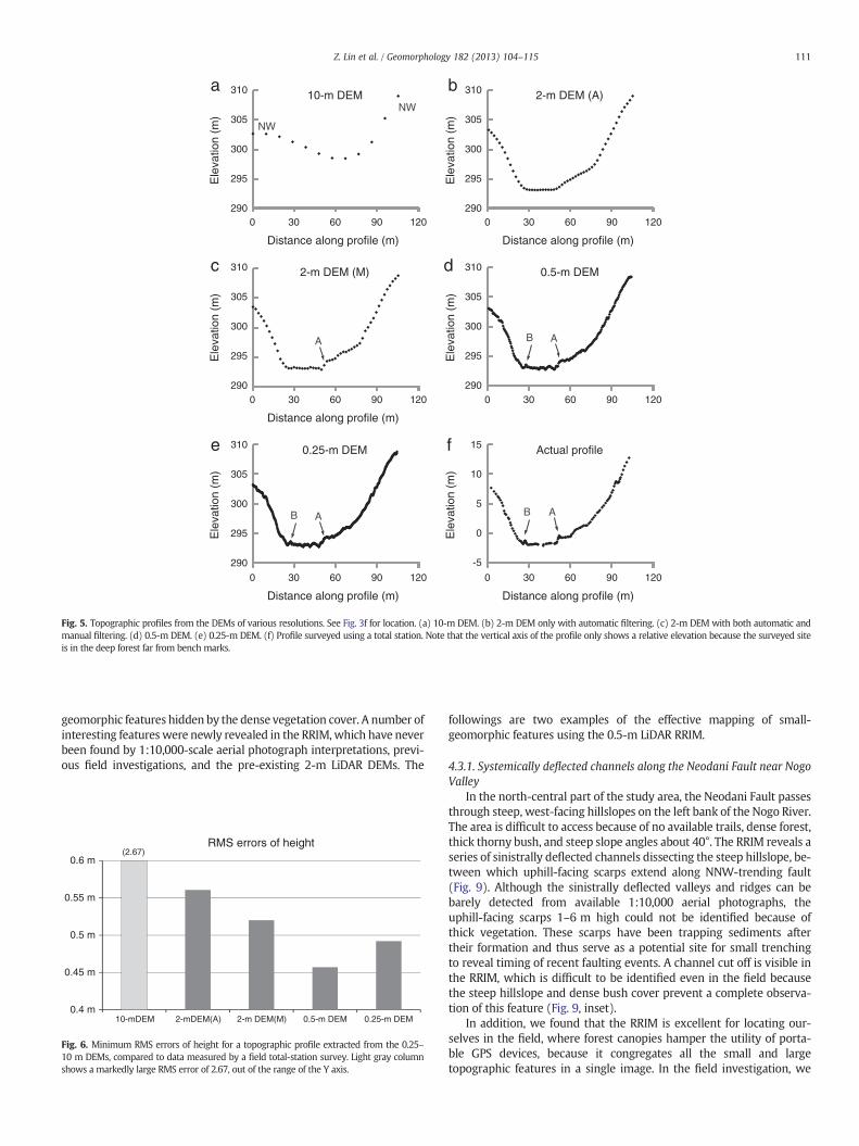
These results indicate that, 0.25 to 0.5 m resolutions of the LiDARDEMs are probably the desired resolution to detect subtle tectonic–geomorphic features. To examine this inference, a field total-stationsurvey was carried out across the trough northeast of the isolatedridge, and topographic profiles from the survey and the differentDEMs were compared (Fig. 5). As the survey site is in a deep forestfar from bench marks, only relative positions and heights were mea-sured, but later, the absolute horizontal position of the profile wasable to be precisely determined using artificial and natural featuresthat are recognized in both the field and LiDAR images. The profileextracted from the 10-m DEMs barely shows the presence of thetrough, and its depth and shape are quite different from actual topog-raphy. The profile of the 2-m DEM (A) excellently represents thedepth and shape of the trough, but the somewhat smoothed profiledoes not allow identification of the subtle topographic breaks, whilethat of the 2-m DEM (M) detects one of topographic breaks of theprotection mounds (A of Fig. 5). Both of the profiles extracted fromthe 0.5-m and 0.25-m DEMs match the field-surveyed actual topogra-phy well, delineating all of the slight topographic breaks.

To quantitatively evaluate the quality of these DEMs, we calculateheight errors of the profiles based on the criterion data from the total sta-tion survey.We prepared the 0.25-m interval “actual profile” by interpo-lation of the total-station data, on the basis of which the minimum RMSerrors of each DEM profiles are searched bymoving the profile vertically(Fig. 6). The error of the 10-m DEM is by far largest (2.67 m) as is ex-pected from the profile's appearance, whereas those of the 2-m DEMsshow a marked improvement down to a value of 0.518–0.558 m. The0.5-m DEM further improves the profile quality (0.456 m), but the qual-ity becomes slightly worse when we go to the finer resolution of the

a

b

c

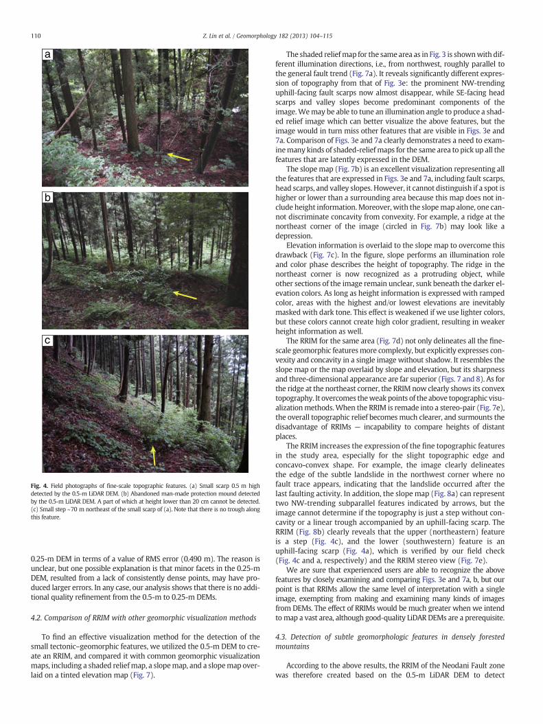
Fig. 4. Field photographs of fine-scale topographic features. (a) Small scarp 0.5 m highdetected by the 0.5-m LiDAR DEM. (b) Abandoned man-made protection mound detectedby the 0.5-m LiDAR DEM. A part of which at height lower than 20 cm cannot be detected.(c) Small step ~70 m northeast of the small scarp of (a). Note that there is no trough alongthis feature.

110 Z. Lin et al. / Geomorphology 182 (2013) 104–115

0.25-m DEM in terms of a value of RMS error (0.490 m). The reason isunclear, but one possible explanation is that minor facets in the 0.25-mDEM, resulted from a lack of consistently dense points, may have pro-duced larger errors. In any case, our analysis shows that there is no addi-tional quality refinement from the 0.5-m to 0.25-m DEMs.

4.2. Comparison of RRIM with other geomorphic visualization methods

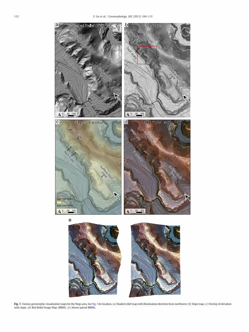
To find an effective visualization method for the detection of thesmall tectonic–geomorphic features, we utilized the 0.5-m DEM to cre-ate an RRIM, and compared it with common geomorphic visualizationmaps, including a shaded reliefmap, a slopemap, and a slopemap over-laid on a tinted elevation map (Fig. 7).

The shaded reliefmap for the samearea as in Fig. 3 is shownwith dif-ferent illumination directions, i.e., from northwest, roughly parallel tothe general fault trend (Fig. 7a). It reveals significantly different expres-sion of topography from that of Fig. 3e: the prominent NW-trendinguphill-facing fault scarps now almost disappear, while SE-facing headscarps and valley slopes become predominant components of theimage.Wemay be able to tune an illumination angle to produce a shad-ed relief image which can better visualize the above features, but theimage would in turn miss other features that are visible in Figs. 3e and7a. Comparison of Figs. 3e and 7a clearly demonstrates a need to exam-inemany kinds of shaded-reliefmaps for the same area to pick up all thefeatures that are latently expressed in the DEM.

The slopemap (Fig. 7b) is an excellent visualization representing allthe features that are expressed in Figs. 3e and 7a, including fault scarps,head scarps, and valley slopes. However, it cannot distinguish if a spot ishigher or lower than a surrounding area because this map does not in-clude height information.Moreover, with the slopemap alone, one can-not discriminate concavity from convexity. For example, a ridge at thenortheast corner of the image (circled in Fig. 7b) may look like adepression.

Elevation information is overlaid to the slope map to overcome thisdrawback (Fig. 7c). In the figure, slope performs an illumination roleand color phase describes the height of topography. The ridge in thenortheast corner is now recognized as a protruding object, whileother sections of the image remain unclear, sunk beneath the darker el-evation colors. As long as height information is expressed with rampedcolor, areas with the highest and/or lowest elevations are inevitablymasked with dark tone. This effect is weakened if we use lighter colors,but these colors cannot create high color gradient, resulting in weakerheight information as well.

The RRIM for the same area (Fig. 7d) not only delineates all the fine-scale geomorphic featuresmore complexly, but explicitly expresses con-vexity and concavity in a single image without shadow. It resembles theslope map or the map overlaid by slope and elevation, but its sharpnessand three-dimensional appearance are far superior (Figs. 7 and 8). As forthe ridge at the northeast corner, the RRIM now clearly shows its convextopography. It overcomes theweak points of the above topographic visu-alizationmethods.When the RRIM is remade into a stereo-pair (Fig. 7e),the overall topographic relief becomes much clearer, and surmounts thedisadvantage of RRIMs — incapability to compare heights of distantplaces.

The RRIM increases the expression of the fine topographic featuresin the study area, especially for the slight topographic edge andconcavo-convex shape. For example, the image clearly delineatesthe edge of the subtle landslide in the northwest corner where nofault trace appears, indicating that the landslide occurred after thelast faulting activity. In addition, the slope map (Fig. 8a) can representtwo NW-trending subparallel features indicated by arrows, but theimage cannot determine if the topography is just a step without con-cavity or a linear trough accompanied by an uphill-facing scarp. TheRRIM (Fig. 8b) clearly reveals that the upper (northeastern) featureis a step (Fig. 4c), and the lower (southwestern) feature is anuphill-facing scarp (Fig. 4a), which is verified by our field check(Fig. 4c and a, respectively) and the RRIM stereo view (Fig. 7e).

We are sure that experienced users are able to recognize the abovefeatures by closely examining and comparing Figs. 3e and 7a, b, but ourpoint is that RRIMs allow the same level of interpretation with a singleimage, exempting from making and examining many kinds of imagesfrom DEMs. The effect of RRIMs would be much greater when we intendtomap a vast area, although good-quality LiDAR DEMs are a prerequisite.

4.3. Detection of subtle geomorphologic features in densely forestedmountains

According to the above results, the RRIM of the Neodani Fault zonewas therefore created based on the 0.5-m LiDAR DEM to detect

310

0E

leva

tion

(m)

10-m DEM 2-m DEM (A)

2-m DEM (M) 0.5-m DEM

0.25-m DEM

-5

0

5

10

15 Actual profile

A A

A A

B

B B

NW

NW305

300

295

290

310

Ele

vatio

n (m

) 305

300

295

290

310

Ele

vatio

n (m

) 305

300

295

290

310

Ele

vatio

n (m

) 305

300

295

290

310

Ele

vatio

n (m

) 305

300

295

290

Ele

vatio

n (m

)

30 60 90 120

Distance along profile (m)

0 30 60 90 120

Distance along profile (m)

0 30 60 90 120

Distance along profile (m)

0 30 60 90 120

0 30 60 90 120

Distance along profile (m)

0 30 60 90 120

Distance along profile (m)

a

c

e f

d

b

Fig. 5. Topographic profiles from the DEMs of various resolutions. See Fig. 3f for location. (a) 10-m DEM. (b) 2-m DEM only with automatic filtering. (c) 2-m DEM with both automatic andmanual filtering. (d) 0.5-m DEM. (e) 0.25-m DEM. (f) Profile surveyed using a total station. Note that the vertical axis of the profile only shows a relative elevation because the surveyed siteis in the deep forest far from bench marks.

111Z. Lin et al. / Geomorphology 182 (2013) 104–115

geomorphic features hidden by the dense vegetation cover. A number ofinteresting featureswere newly revealed in the RRIM,which have neverbeen found by 1:10,000-scale aerial photograph interpretations, previ-ous field investigations, and the pre-existing 2-m LiDAR DEMs. The

(2.67)0.6 m

10-mDEM 2-mDEM(A) 2-m DEM(M) 0.5-m DEM 0.25-m DEM

0.55 m

0.5 m

0.45 m

0.4 m

RMS errors of height

Fig. 6. Minimum RMS errors of height for a topographic profile extracted from the 0.25–10 m DEMs, compared to data measured by a field total-station survey. Light gray columnshows a markedly large RMS error of 2.67, out of the range of the Y axis.

followings are two examples of the effective mapping of small-geomorphic features using the 0.5-m LiDAR RRIM.

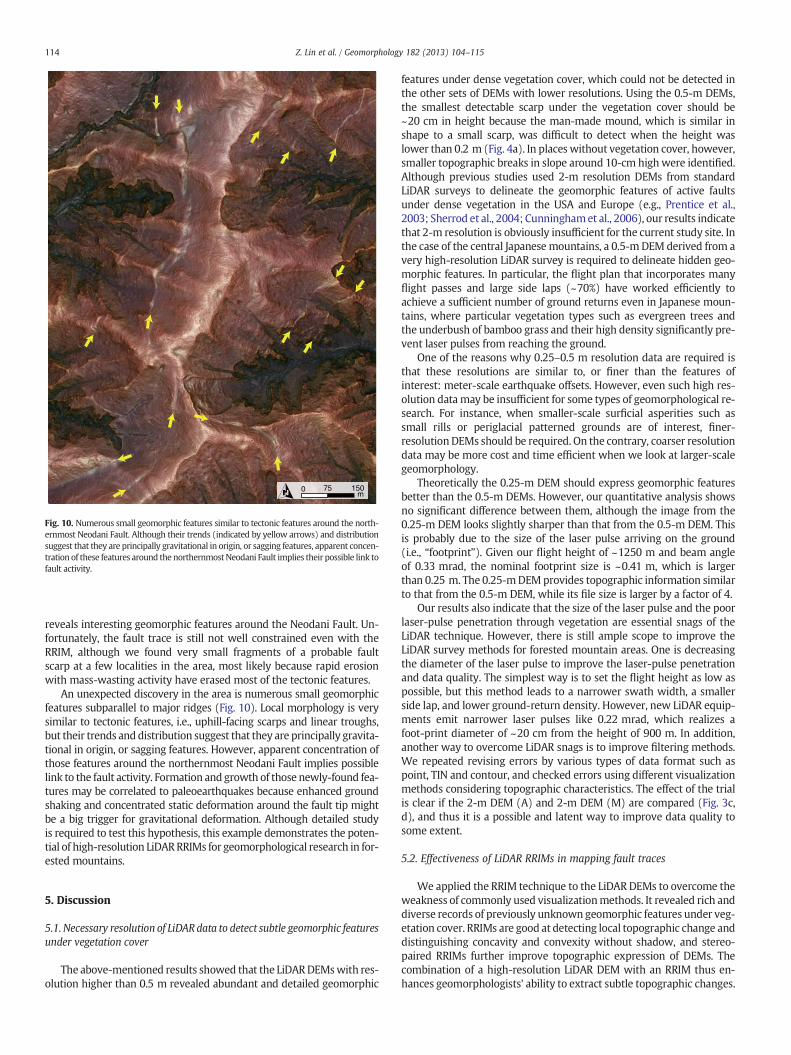
4.3.1. Systemically deflected channels along the Neodani Fault near NogoValley

In the north-central part of the study area, the Neodani Fault passesthrough steep, west-facing hillslopes on the left bank of the Nogo River.The area is difficult to access because of no available trails, dense forest,thick thorny bush, and steep slope angles about 40°. The RRIM reveals aseries of sinistrally deflected channels dissecting the steep hillslope, be-tween which uphill-facing scarps extend along NNW-trending fault(Fig. 9). Although the sinistrally deflected valleys and ridges can bebarely detected from available 1:10,000 aerial photographs, theuphill-facing scarps 1–6 m high could not be identified because ofthick vegetation. These scarps have been trapping sediments aftertheir formation and thus serve as a potential site for small trenchingto reveal timing of recent faulting events. A channel cut off is visible inthe RRIM, which is difficult to be identified even in the field becausethe steep hillslope and dense bush cover prevent a complete observa-tion of this feature (Fig. 9, inset).

In addition, we found that the RRIM is excellent for locating our-selves in the field, where forest canopies hamper the utility of porta-ble GPS devices, because it congregates all the small and largetopographic features in a single image. In the field investigation, we

c d

a b

e

Fig. 7. Various geomorphic visualizationmaps for theNogo area. See Fig. 1 for location. (a) Shaded reliefmapwith illumination direction fromnorthwest. (b) Slopemap. (c)Overlay of elevationwith slope. (d) Red Relief Image Map (RRIM). (e) Stereo-paired RRIMs.

112 Z. Lin et al. / Geomorphology 182 (2013) 104–115

15 30m

0 15 30m

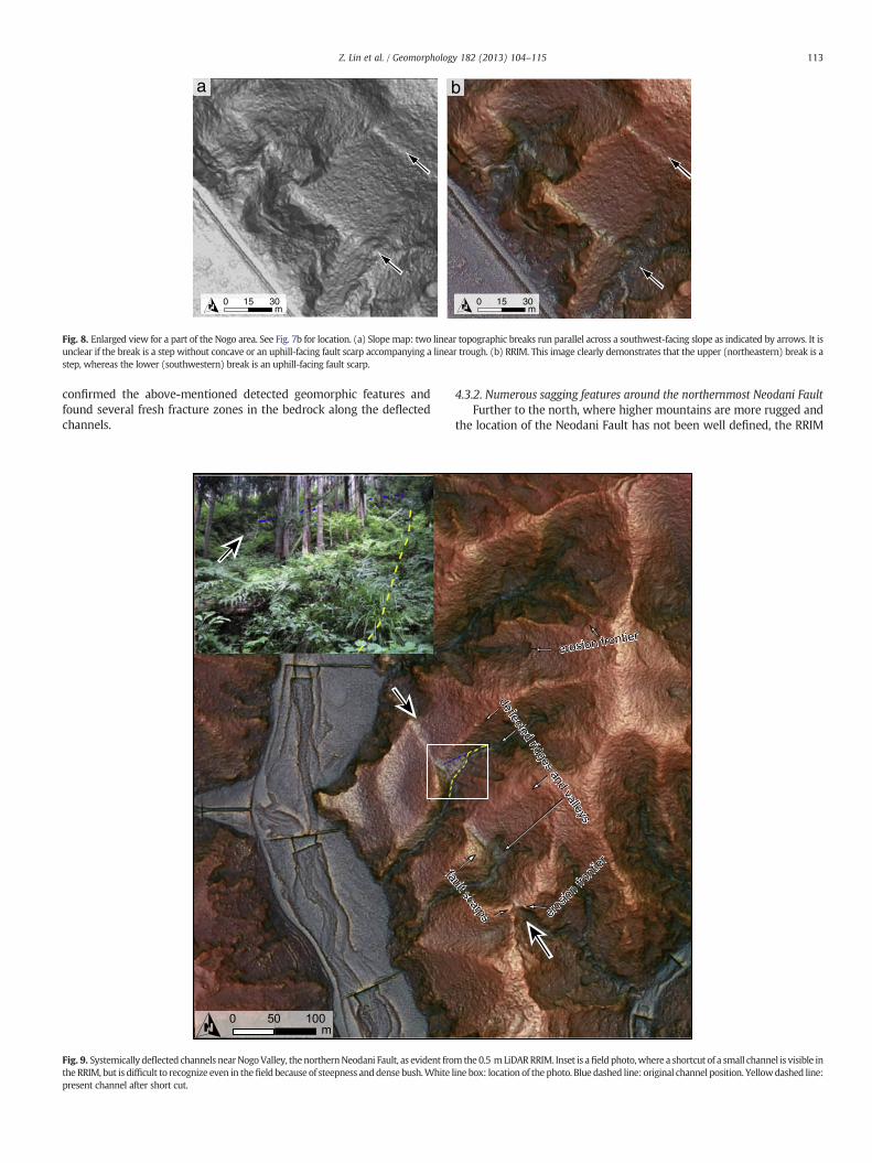
ba

Fig. 8. Enlarged view for a part of the Nogo area. See Fig. 7b for location. (a) Slope map: two linear topographic breaks run parallel across a southwest-facing slope as indicated by arrows. It isunclear if the break is a step without concave or an uphill-facing fault scarp accompanying a linear trough. (b) RRIM. This image clearly demonstrates that the upper (northeastern) break is astep, whereas the lower (southwestern) break is an uphill-facing fault scarp.

113Z. Lin et al. / Geomorphology 182 (2013) 104–115

confirmed the above-mentioned detected geomorphic features andfound several fresh fracture zones in the bedrock along the deflectedchannels.

Fig. 9. Systemically deflected channels nearNogoValley, thenorthernNeodani Fault, as evident frothe RRIM, but is difficult to recognize even in thefield because of steepness anddense bush.White lpresent channel after short cut.

4.3.2. Numerous sagging features around the northernmost Neodani FaultFurther to the north, where higher mountains are more rugged and

the location of the Neodani Fault has not been well defined, the RRIM

mthe0.5 mLiDARRRIM. Inset is afield photo,where a shortcut of a small channel is visible inine box: location of the photo. Blue dashed line: original channel position. Yellowdashed line:

15075m

0

Fig. 10. Numerous small geomorphic features similar to tectonic features around the north-ernmost Neodani Fault. Although their trends (indicated by yellow arrows) and distributionsuggest that they are principally gravitational in origin, or sagging features, apparent concen-tration of these features around the northernmost Neodani Fault implies their possible link tofault activity.

114 Z. Lin et al. / Geomorphology 182 (2013) 104–115

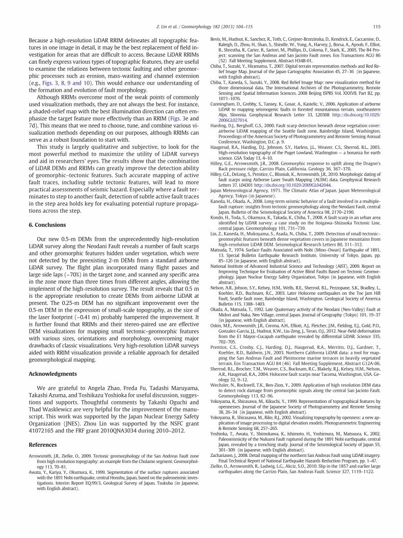
reveals interesting geomorphic features around the Neodani Fault. Un-fortunately, the fault trace is still not well constrained even with theRRIM, although we found very small fragments of a probable faultscarp at a few localities in the area, most likely because rapid erosionwith mass-wasting activity have erased most of the tectonic features.

An unexpected discovery in the area is numerous small geomorphicfeatures subparallel to major ridges (Fig. 10). Local morphology is verysimilar to tectonic features, i.e., uphill-facing scarps and linear troughs,but their trends and distribution suggest that they are principally gravita-tional in origin, or sagging features. However, apparent concentration ofthose features around the northernmost Neodani Fault implies possiblelink to the fault activity. Formation and growth of those newly-found fea-tures may be correlated to paleoearthquakes because enhanced groundshaking and concentrated static deformation around the fault tip mightbe a big trigger for gravitational deformation. Although detailed studyis required to test this hypothesis, this example demonstrates the poten-tial of high-resolution LiDARRRIMs for geomorphological research in for-ested mountains.

5. Discussion

5.1. Necessary resolution of LiDAR data to detect subtle geomorphic featuresunder vegetation cover

The above-mentioned results showed that the LiDARDEMswith res-olution higher than 0.5 m revealed abundant and detailed geomorphic

features under dense vegetation cover, which could not be detected inthe other sets of DEMs with lower resolutions. Using the 0.5-m DEMs,the smallest detectable scarp under the vegetation cover should be~20 cm in height because the man-made mound, which is similar inshape to a small scarp, was difficult to detect when the height waslower than 0.2 m (Fig. 4a). In places without vegetation cover, however,smaller topographic breaks in slope around 10-cm highwere identified.Although previous studies used 2-m resolution DEMs from standardLiDAR surveys to delineate the geomorphic features of active faultsunder dense vegetation in the USA and Europe (e.g., Prentice et al.,2003; Sherrod et al., 2004; Cunninghamet al., 2006), our results indicatethat 2-m resolution is obviously insufficient for the current study site. Inthe case of the central Japanesemountains, a 0.5-m DEM derived from avery high-resolution LiDAR survey is required to delineate hidden geo-morphic features. In particular, the flight plan that incorporates manyflight passes and large side laps (~70%) have worked efficiently toachieve a sufficient number of ground returns even in Japanese moun-tains, where particular vegetation types such as evergreen trees andthe underbush of bamboo grass and their high density significantly pre-vent laser pulses from reaching the ground.

One of the reasons why 0.25–0.5 m resolution data are required isthat these resolutions are similar to, or finer than the features ofinterest: meter-scale earthquake offsets. However, even such high res-olution datamay be insufficient for some types of geomorphological re-search. For instance, when smaller-scale surficial asperities such assmall rills or periglacial patterned grounds are of interest, finer-resolutionDEMs should be required. On the contrary, coarser resolutiondata may be more cost and time efficient when we look at larger-scalegeomorphology.

Theoretically the 0.25-m DEM should express geomorphic featuresbetter than the 0.5-m DEMs. However, our quantitative analysis showsno significant difference between them, although the image from the0.25-m DEM looks slightly sharper than that from the 0.5-m DEM. Thisis probably due to the size of the laser pulse arriving on the ground(i.e., “footprint”). Given our flight height of ~1250 m and beam angleof 0.33 mrad, the nominal footprint size is ~0.41 m, which is largerthan 0.25 m. The 0.25-mDEMprovides topographic information similarto that from the 0.5-m DEM, while its file size is larger by a factor of 4.

Our results also indicate that the size of the laser pulse and the poorlaser-pulse penetration through vegetation are essential snags of theLiDAR technique. However, there is still ample scope to improve theLiDAR survey methods for forested mountain areas. One is decreasingthe diameter of the laser pulse to improve the laser-pulse penetrationand data quality. The simplest way is to set the flight height as low aspossible, but this method leads to a narrower swath width, a smallerside lap, and lower ground-return density. However, new LiDAR equip-ments emit narrower laser pulses like 0.22 mrad, which realizes afoot-print diameter of ~20 cm from the height of 900 m. In addition,another way to overcome LiDAR snags is to improve filtering methods.We repeated revising errors by various types of data format such aspoint, TIN and contour, and checked errors using different visualizationmethods considering topographic characteristics. The effect of the trialis clear if the 2-m DEM (A) and 2-m DEM (M) are compared (Fig. 3c,d), and thus it is a possible and latent way to improve data quality tosome extent.

5.2. Effectiveness of LiDAR RRIMs in mapping fault traces

We applied the RRIM technique to the LiDAR DEMs to overcome theweakness of commonly used visualizationmethods. It revealed rich anddiverse records of previously unknown geomorphic features under veg-etation cover. RRIMs are good at detecting local topographic change anddistinguishing concavity and convexity without shadow, and stereo-paired RRIMs further improve topographic expression of DEMs. Thecombination of a high-resolution LiDAR DEM with an RRIM thus en-hances geomorphologists' ability to extract subtle topographic changes.

115Z. Lin et al. / Geomorphology 182 (2013) 104–115

Because a high-resolution LiDAR RRIM delineates all topographic fea-tures in one image in detail, it may be the best replacement of field in-vestigation for areas that are difficult to access. Because LiDAR RRIMscan finely express various types of topographic features, they are usefulto examine the relations between tectonic faulting and other geomor-phic processes such as erosion, mass-wasting and channel extension(e.g., Figs. 3, 8, 9 and 10). This would enhance our understanding ofthe formation and evolution of fault morphology.

Although RRIMs overcome most of the weak points of commonlyused visualization methods, they are not always the best. For instance,a shaded-relief map with the best illumination direction can often em-phasize the target feature more effectively than an RRIM (Figs. 3e and7d). This means that we need to choose, tune, and combine various vi-sualization methods depending on our purposes, although RRIMs canserve as a robust foundation to start with.

This study is largely qualitative and subjective, to look for themost powerful method to maximize the utility of LiDAR surveysand aid in researchers' eyes. The results show that the combinationof LiDAR DEMs and RRIMs can greatly improve the detection abilityof geomorphic–tectonic features. Such accurate mapping of activefault traces, including subtle tectonic features, will lead to morepractical assessments of seismic hazard. Especially where a fault ter-minates to step to another fault, detection of subtle active fault tracesin the step area holds key for evaluating potential rupture propaga-tions across the step.

6. Conclusions

Our new 0.5-m DEMs from the unprecedentedly high-resolutionLiDAR survey along the Neodani Fault reveals a number of fault scarpsand other geomorphic features hidden under vegetation, which werenot detected by the preexisting 2-m DEMs from a standard airborneLiDAR survey. The flight plan incorporated many flight passes andlarge side laps (~70%) in the target zone, and scanned any specific areain the zone more than three times from different angles, allowing theimplement of the high-resolution survey. The result reveals that 0.5 mis the appropriate resolution to create DEMs from airborne LiDAR atpresent. The 0.25-m DEM has no significant improvement over the0.5-m DEM in the expression of small-scale topography, as the size ofthe laser footprint (~0.41 m) probably hampered the improvement. Itis further found that RRIMs and their stereo-paired use are effectiveDEM visualizations for mapping small tectonic–geomorphic featureswith various sizes, orientations and morphology, overcoming majordrawbacks of classic visualizations. Very high-resolution LiDAR surveysaided with RRIM visualization provide a reliable approach for detailedgeomorphological mapping.

Acknowledgments

We are grateful to Angela Zhao, Freda Fu, Tadashi Maruyama,Takashi Azuma, and Toshikazu Yoshioka for useful discussion, sugges-tions and supports. Thoughtful comments by Takashi Oguchi andThad Wasklewicz are very helpful for the improvement of the manu-script. This work was supported by the Japan Nuclear Energy SafetyOrganization (JNES). Zhou Lin was supported by the NSFC grant41072165 and the FRF grant 2010QNA3034 during 2010–2012.

References

Arrowsmith, J.R., Zielke, O., 2009. Tectonic geomorphology of the San Andreas Fault zonefromhigh resolution topography: an example from the Cholame segment. Geomorphol-ogy 113, 70–81.

Awata, Y., Kariya, Y., Okumura, K., 1999. Segmentation of the surface ruptures associatedwith the 1891Nobi earthquake, central Honshu, Japan, based on the paleoseismic inves-tigations. Interim Report EQ/99/3, Geological Survey of Japan, Tsukuba (in Japanese,with English abstract).

Bevis, M., Hudnut, K., Sanchez, R., Toth, C., Grejner-Brzezinska, D., Kendrick, E., Caccamise, D.,Raleigh, D., Zhou, H., Shan, S., Shindle, W., Yong, A., Harvey, J., Borsa, A., Ayoub, F., Elliot,B., Shrestha, R., Carter, B., Sartori, M., Phillips, D., Coloma, F., Stark, K., 2005. The B4 Pro-ject: scanning the San Andreas and San Jacinto Fault zones. Eos Transactions AGU 86(52) Fall Meeting Supplement, Abstract H34B-01.

Chiba, T., Suzuki, Y., Hiramatsu, T., 2007. Digital terrain representation methods and Red Re-lief Image Map. Journal of the Japan Cartographic Association 45, 27–36 (in Japanese,with English abstract).

Chiba, T., Kaneda, S., Suzuki, Y., 2008. Red Relief Image Map: new visualization method forthree dimensional data. The International Archives of the Photogrammetry, RemoteSensing and Spatial Information Sciences. 2008 Beijing ISPRS Vol. XXXVII. Part B2, pp.1071–1076.

Cunningham, D., Grebby, S., Tansey, K., Gosar, A., Kastelic, V., 2006. Application of airborneLiDAR to mapping seismogenic faults in forested mountainous terrain, southeasternAlps, Slovenia. Geophysical Research Letter 33, L20308 http://dx.doi.org/10.1029/2006GL027014.

Harding, D.J., Berghoff, G.S., 2000. Fault scarp detection beneath dense vegetation cover:airborne LiDAR mapping of the Seattle fault zone, Bainbridge Island, Washington.Proceedings of the American Society of Photogrammetry and Remote Sensing AnnualConference, Washington, D.C. p. 9.

Haugerud, R.A., Harding, D.J., Johnson, S.Y., Harless, J.L., Weaver, C.S., Sherrod, B.L., 2003.High-resolution topography of the Puget Lowland, Washington — a bonanza for earthscience. GSA Today 13, 4–10.

Hilley, G.E., Arrowsmith, J.R., 2008. Geomorphic response to uplift along the Dragon'sBack pressure ridge, Carrizo Plain, California. Geology 36, 367–370.

Hilley, G.E., DeLong, S., Prentice, C., Blisniuk, K., Arrowsmith, J.R., 2010. Morphologic dating offault scarps using Airborne Laser Swath Mapping (ALSM) data. Geophysical ResearchLetters 37, L04301 http://dx.doi.org/10.1029/2009GL042044.

Japan Meteorological Agency, 1971. The Climatic Atlas of Japan. Japan MeteorologicalAgency, Tokyo (in Japanese).

Kaneda, H., Okada, A., 2008. Long-term seismic behavior of a fault involved in a multiple-fault rupture: insights from tectonic geomorphology along the Neodani Fault, centralJapan. Bulletin of the Seismological Society of America 98, 2170–2190.

Kondo, H., Toda, S., Okamura, K., Takada, K., Chiba, T., 2008. A fault scarp in an urban areaidentified by LiDAR survey: a case study on the Itoigawa–Shizuoka Tectonic Line,central Japan. Geomorphology 101, 731–739.

Lin, Z., Kaneda, H., Mukoyama, S., Asada, N., Chiba, T., 2009. Detection of small tectonic–geomorphic features beneath dense vegetation covers in Japanese mountains fromhigh-resolution LiDAR DEM. Seismological Research Letters 80, 311–312.

Matsuda, T., 1974. Surface Faults Associated with Nobi (Mino–Owari) Earthquake of 1891,13. Special Bulletin Earthquake Research Institute, University of Tokyo, Japan, pp.85–126 (in Japanese, with English abstract).

National Institute of Advanced Industrial Science and Technology (AIST), 2009. Report onImproving Technique for Evaluation of Active Blind Faults Based on Tectonic Geomor-phology. Japan Nuclear Energy Safety Organization, Tokyo (in Japanese, with Englishabstract).

Nelson, A.R., Johson, S.Y., Kelsey, H.M., Wells, R.E., Sherrod, B.L., Pezzopane, S.K., Bradley, L.,Koehler, R.D., Buchnam, R.C., 2003. Later Holocene earthquakes on the Toe Jam HillFault, Seattle fault zone, Bainbridge Island, Washington. Geological Society of AmericaBulletin 115, 1388–1403.

Okada, A., Matsuda, T., 1992. Late Quaternary activity of the Neodani (Neo-Valley) Fault atMidori and Naka, Neo Village, central Japan. Journal of Geography (Tokyo) 101, 19–37(in Japanese, with English abstract).

Oskin, M.E., Arrowsmith, J.R., Corona, A.H., Elliott, A.J., Fletcher, J.M., Fielding, E.J., Gold, P.O.,Gonzalez-Garcia, J.J., Hudnut, K.W., Liu-Zeng, J., Teran, O.J., 2012. Near-field deformationfrom the E1 Mayor–Cucapah earthquake revealed by differential LiDAR. Science 335,702–705.

Prentice, C.S., Crosby, C.J., Harding, D.J., Haugerud, R.A., Merritts, D.J., Gardner, T.,Koehler, R.D., Baldwin, J.N., 2003. Northern California LiDAR data: a tool for map-ping the San Andreas Fault and Pleistocene marine terraces in heavily vegetatedterrain. Eos Transaction AGU 84 (46) Fall Meeting Supplement, Abstract G12A-06.

Sherrod, B.L., Brocher, T.M., Weaver, C.S., Bucknam, R.C., Blakely, R.J., Kelsey, H.M., Nelson,A.R., Haugerud, R.A., 2004. Holocene fault scarps near Tacoma, Washington, USA. Ge-ology 32, 9–12.

Wechsler, N., Rockwell, T.K., Ben-Zion, Y., 2009. Application of high resolution DEM datato detect rock damage from geomorphic signals along the central San Jacinto Fault.Geomorphology 113, 82–96.

Yokoyama, R., Shirasawa, M., Kikuchi, Y., 1999. Representation of topographical features byopennesses. Journal of the Japanese Society of Photogrammetry and Remote Sensing38, 26–34 (in Japanese, with English abstract).

Yokoyama, R., Shirasawa, M., Rike, R.J., 2002. Visualizing topography by openness: a new ap-plication of image processing to digital elevation models. Photogrammetric Engineering& Remote Sensing 68, 257–265.

Yoshioka, T., Awata, Y., Shimokawa, K., Ishimoto, H., Yoshimura, M., Matsuura, K., 2002.Paleoseismicity of the Nukumi Fault ruptured during the 1891 Nobi earthquake, centralJapan, revealed by a trenching study. Journal of the Seismological Society of Japan 55,301–309 (in Japanese, with English abstract).

Zachariasen, J., 2008. Detail mapping of the northern San Andreas Fault using LiDAR imagery.Final Technical Report of National Earthquake Hazards Reduction Program, pp. 1–47.

Zielke, O., Arrowsmith, R., Ludwig, L.G., Akciz, S.O., 2010. Slip in the 1857 and earlier largeearthquakes along the Carrizo Plain, San Andreas Fault. Science 327, 1119–1122.