Embed Size (px)
Citation preview
Università degli Studi di PadovaDipartimento di Fisica Galileo Galilei
Corso di Laurea Magistrale in Fisica
D E T E C T I N G C A U S A L I T Y I N C O M P L E XS Y S T E M
Relatore:Dott. Samir Suweiss
Laureando:Jacopo Schiavon
September 2017

A B S T R A C T
In this work, recent and classical results on causality detection and predicabil-ity of a complex system have been reviewed critically. In the �rst part, I haveextensively studied the Convergent Cross Mapping method [1] and I tested itin cases of particular interest. I have also confronted this approach with theclassical Granger framework for causality [2]. A study with a simulated Lotka-Volterra model has shown certain limits of this method, and I have obtainedcounterintuitive results.
In the second part of the work, I have made a description of the Analogmethod [3] to perform prediction on complex systems. I have also studied thetheorem on which this approach is rooted, the Takens’ theorem. Moreover, wehave investigated the main limitation of this approach, known as the curse of di-mensionality: when the system increases in dimensionality the number of dataneeded to obtain su�ciently accurate predictions scales exponentially with di-mension. Additionally, �nding the e�ective dimension of a complex system isstill an open problem. I have presented methods to estimate the e�ective di-mension of the attractor of dynamical systems known as Grassberger-Procacciaalgorithm and his extensions [4]. Finally, I have tested all these data driven ma-chineries to a well-studied dynamical system, i.e. the Lorenz system, �ndingthat the theoretical results are con�rmed and the data needed scales asN ∼ εd.
iii


C O N T E N T S
introduction 1
1 causality and convergent cross-mapping 31.1 Granger causality and Transfer Entropy 41.2 Convergent Cross-Mapping 81.3 Problem of Convergent Cross-Mapping and extensions 15
2 applications of convergent cross-mapping 172.1 Description of the system 172.2 Small carrying capacity 202.3 Big carrying capacity 252.4 Summary 27
3 method of analogs and dimensionality 293.1 Method of analogs 303.2 Takens’ theorem and prediction 323.3 Statistical di�culty in method of analogs 37
4 numerical approach to the curse of dimensionality 434.1 Grassberger-Procaccia algorithm for the correlation dimension 434.2 Center of Mass prediction algorithm 45
5 conclusions 47
a proof of takens’ theorem. 49
bibliography 51
v

A C R O N Y M S
CCM Convergent Cross-Mapping
COM Center of Mass
DoF Degrees of Freedom
GC Granger Causality
LL Local Linear
LV Lotka-Volterra
MLE Maximal Lyapunov Exponent
PAI Pairwise Asymmetric Inference
PCC Pearson Correlation Coe�cient
SDE Stochastic Di�erential Equation
TE Transfer Entropy
vi
I N T R O D U C T I O N
The aim of this work is to study how to infer information on a complex dy-namical system only from data and without explicitly knowing the underlyingdynamics nor the relevant parameters of the systems.
When trying to predict the future of a system, one has to choose one of twomain approach to the problem: the �rst is to understand the laws that governthe evolution of the system (if any) thus creating theoretical models that canexplain and reproduce the observed system behaviour - described by data - andcan also make predictions on its evolution, known as generative models [5, 6].The alternative approach is more inductive and it attempts to predict the sys-tem evolution by inferring statistical models directly from the data, in this casecalled discriminative models [5, 6]. In this second approach one does not care ofcauses, but it only exploits statistical correlations to make predictions.
The scienti�c method used extensively in physics, from Galileo onward, hasalways been built upon the �rst kind of strategy. Observations, experiments andmathematical theoretical frameworks are used to to understand the fundamen-tal and universal laws that govern the inanimate matter world. They are thustranslated in models with parameters, and data are used to estimate them andto make new predictions. Finally experiments are done to falsify these models,closing the never closed loop of a scienti�c discovery. This has been, for exam-ple, the case of the Standard Model, with the recent discover of Higgs Boson[7]: the Standard Model have been developed in the second half of ’900, andHiggs has published his paper in 1964 [8], a whole 50 years before the actualexperimental con�rm of the particle (made in 2012 at LHC [9, 10]).
In fact, physicists have always been skeptical about the second - data based- inductive approach. Indeed, Physics emerged from the awareness that mathe-matics could be used as a language to reason about and describe natural world[11]. The goal of physics has been to isolate the causation phenomena describedby mathematical models that are able to generate synthetic data prior to any ob-servations. In general, physicists do not think of these models being generativebecause what else could they be? But it is a choice nonetheless. Surely, the de-velopment of theoretical physics has been allowed by the possibility to accessto the most outstanding experiments in science that thanks to the relentlesse�orts of experimental physicists have reached a precision incomparable withother branches of science. In fact, when physicists confront problems in biol-ogy, economics and social sciences, the available data are of a poor quality andwith a very complex structure. And in most of these cases we are very far fromidentifying �rst principle laws that govern the dynamics of these systems.
Conversely, many successful applications of arti�cial intelligence use modelsessentially as black boxes: they map a set of known inputs and outputs (trainingdata) by determining a set of parameters that give good performance when
1

2 introduction
generalized to pairs of input and output (test data) not used in the training.In recent years, therefore, the always increasing amount of data available toscientist is leading some very deep question about the approach that should beused when studying complex systems.
It is of great interest, then, the possibility of infer at least some properties ofthe system without the needs to create the full model and �t it to data, or atleast to understand when this task is at least applicable. A very important andwidespread example of this approach are neural networks: by using a set oftechniques that are best thought of as a supervised learning approach, treatingthe experimental/observational data as a direct input, which is then used toiteratively improve the prediction power of the statistical model.
outline of the work
The approach I will present in this work is a compromise between the abilityto predict and the desire to gain some insight about the structure and the pro-cesses driving the system dynamics. For example, one would like to understandif there are variables more "important" than others, or if some of them have afundamental role in predicting others. In this thesis, I will thus focus on twodistinct problems: the detection of causal relationship and the determinationof e�ective variables’ number (i.e. the dimensionality of the system), giving uscrucial information for the understanding of the analyzed system.
Accordingly the thesis is divided in two main parts. The �rst one is aboutthe concept of causality: what it is and methods to measure and detect it. Here(Chapter 1) I have �rstly made a survey of the methods known up to now, focus-ing in one of the newer and more promising one, which is Convergent Cross-Mapping (CCM). Then (in Chapter 2) I have studied a toy Lotka-Volterra (LV)-likemodel exploring what happens to the causality predicted by CCM method vari-ating some of its parameters.
The second part, instead, focus on methods to estimate the number of e�ec-tive variables, in order to give an hint about predictability. I devote a chapter(Chapter 3 on page 29) for a theoretical review of the tools used to estimate thedimensionality of a system (through an approach introduced by Grassbergerand Procaccia [4]) and to make prediction by means of the historical record ofthe system (the so called Analog method [3]), and another one (Chapter 4 onpage 43) where I apply this approach on a complex system.

1G E N E R A L D E F I N I T I O N O FC A U S A L I T Y , G R A N G E R C A U S A L I T YA N D C O N V E R G E N TC R O S S - M A P P I N G M E T H O D
In this chapter I will �rst introduce the concept of causality in some of its manyvariants, then focusing on the description of CCM [1] method and its generaliza-tions [12].
the concept of causality
While causality is a concept that is widespread in common language, it did nothad a consistent formal de�nition for time series until half of the ’900, and evennow there are many variant of the same concept.
The problem is that, while we have a grasp of what we mean by saying that acertain phenomena cause another, putting these words in a more formal mathe-matical language is not an easy tasks. When dealing with events that occurs intime, probably the �rst relevant problem is to understand how one time seriescan be related to the others. This problem was partially solved by Galton andPearson with the introduction of correlation [13].
Even if correlation is a good way to measure similarity between two time se-ries, to imply causation from correlation is a logical fallacia, as was clear even toPearson itself (see [14] for a detailed discussion of this problem from the pointof view of Pearson and his student Yule). This problem was �nally overcameby Granger in 1969 [2], with a big perspective shift: the causal relation mustcome from the ability to use informations encoded in one series to make state-ments about the other. In this sense, Granger idea was the �rst step toward aninformation theory framework, even though the tools used in his de�nition arepurely statistical.
A possible and intuitive de�nition for a phenomenon to cause another oneis that the former (cause) should pass some kind of information to the latter(e�ect), thus creating a directed interaction between the two. Another way ofthinking this concept is that from the (cause) we should be able to predict insome way the (e�ect). Finally, changing perspective, one can think that the e�ect
3

4 causality and convergent cross-mapping
should help the prediction, given that it must in some way encode informationsabout the cause. These three naively presented approach to causality are themost used ones, de�ning the three main categories of techniques currently usedto make causal inference: Transfer Entropy, Granger Causality and ConvergentCross Mapping.
granger causality and transfer entropy
I will begin this survey with Granger Causality (GC), introduced in 1969 [2] andbased upon Wiener’s work [15] about predictability. Informally, given X and Ytwo stationary stochastic variables, Y is said to Granger cause X if the ability topredict X is improved by incorporating information about Y.
Rephrased, given two time series, under the GC framework, one is consideredthe cause and one the e�ect if informations encoded in the former are helpful inorder to predict the latter. This is consistent with our experience, but we wantto formalize this concept.
In order to give a formal de�nition we have to �rst introduce some notation.Let denote Xt as a stationary stochastic process and Xt the set of past values ofXt, which is to say the set {Xt−j} with j ∈ {1, 2, . . . ,∞}. We de�ne also Ut tobe all the information in universe accumulated until time t andUt− Yt all thisinformation apart from a speci�ed series Yt. Moreover, denoted the predictionofAt using the setBtwith Pt(A|B), we de�neσ2(A|B) to be the variance of theseries of predictive error εt(A|B) = At − Pt(A|B), σ2(A|B) = 〈εt(A|B)2〉−〈εt(A|B)〉2.
Then we can write the following de�nition:
1.1 Definition (Granger Causality). LetXt and Yt be two stationary stochas-Granger de�nition of causalitytic processes. If and only if σ2(X|U) < σ2(X|U− Y), then we say that YtGranger cause Xt (which we will indicate as Yt
Grg−→ Xt).
This de�nition means that we improve our ability of predicting X (measuredby the variance of the series of predictive errors σ2) using all the informationin the universe with respect to the prediction obtained excluding informationabout Y.
This very same de�nition can be extended naturally to the concept of feed-back, which means that Xt
Grg−→ Yt and at the same time YtGrg−→ Xt:
1.2 Definition (Granger feedback). We say that feedbak between Xt and YtGranger de�nition of feedback
is occurring (XtGrg←→ Yt) if:
• σ2(X|U) < σ2(X|U− Y) and• σ2(Y|U) < σ2(Y|U−X).
The last concept that is interesting for our scope is the causality lag, whichrepresent the time that occurs for a series Y to cause X. Technically, it is de�nedas:
1.1 granger causality and transfer entropy 5
1.3 Definition (Granger Causality lag). If YtGrg−→ Xt, we de�ne the causal- Granger de�nition of causality
lagity lag m to be the least value k such that σ2(X|U− Y(k)) < σ2(X|U− Y(k+
1)), which means that knowing the values Yt−j for j = 0, 1, . . . ,m− 1 doesnot improve our ability to predict Xt.
This de�nitions are probably the most used for causality in a wide varietyof �elds from economy and �nance to demography, social science and biomed-ical applications (for some interesting, even if far from the scope of this work,examples see [16–18]).
transfer entropy
Transfer Entropy (TE) is an information theoretic measure that quantify theoverlap of information content of two systems and, more importantly, the dy-namics of information transport, thus exploiting eventual relation of causality.It has been introduced by Schreiber [19] in 2000 and ever since has been used ina wide range of applications (see [20] for an example of application of transferentropy to the study of Ising model).
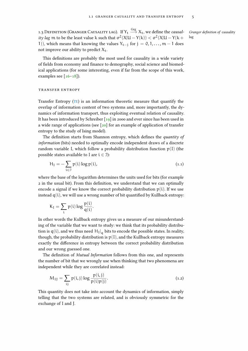
The de�nition starts from Shannon entropy, which de�nes the quantity ofinformation (bits) needed to optimally encode independent draws of a discreterandom variable I, which follow a probability distribution function p(I) (thepossible states available to I are i ∈ I):
HI = −∑i∈I
p(i) logp(i), (1.1)
where the base of the logarithm determines the units used for bits (for example2 in the usual bit). From this de�nition, we understand that we can optimallyencode a signal if we know the correct probability distribution p(i). If we useinstead q(i), we will use a wrong number of bit quanti�ed by Kullback entropy:
KI =∑i
p(i) logp(i)
q(i).
In other words the Kullback entropy gives us a measure of our misunderstand-ing of the variable that we want to study: we think that its probability distribu-tion is q(i), and we thus need HI|q bits to encode the possible states. In reality,though, the probability distribution is p(I), and the Kullback entropy measuresexactly the di�erence in entropy between the correct probability distributionand our wrong guessed one.
The de�nition of Mutual Information follows from this one, and representsthe number of bit that we wrongly use when thinking that two phenomena areindependent while they are correlated instead:
MIJ =∑ij
p(i, j) logp(i, j)p(i)p(j)
. (1.2)
This quantity does not take into account the dynamics of information, simplytelling that the two systems are related, and is obviously symmetric for theexchange of I and J.
6 causality and convergent cross-mapping
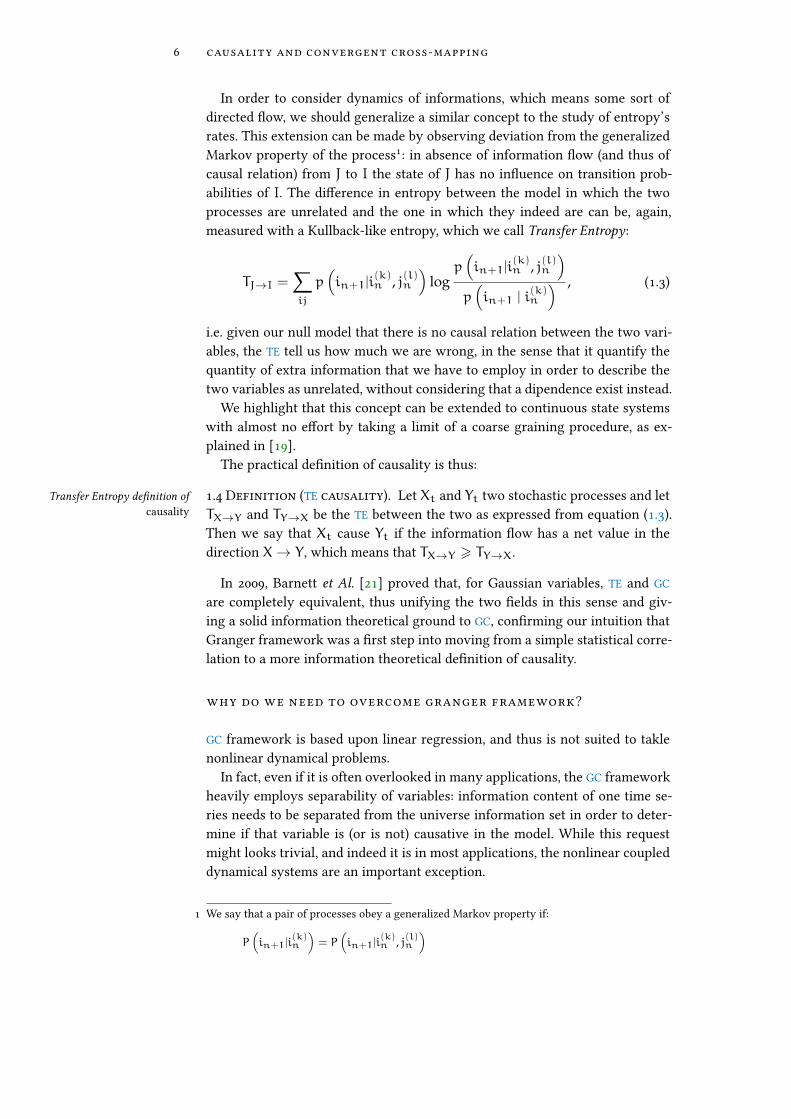
In order to consider dynamics of informations, which means some sort ofdirected �ow, we should generalize a similar concept to the study of entropy’srates. This extension can be made by observing deviation from the generalizedMarkov property of the process1: in absence of information �ow (and thus ofcausal relation) from J to I the state of J has no in�uence on transition prob-abilities of I. The di�erence in entropy between the model in which the twoprocesses are unrelated and the one in which they indeed are can be, again,measured with a Kullback-like entropy, which we call Transfer Entropy:
TJ→I =∑ij
p(in+1|i
(k)n , j(l)n
)log
p(in+1|i
(k)n , j(l)n
)p(in+1 | i
(k)n
) , (1.3)
i.e. given our null model that there is no causal relation between the two vari-ables, the TE tell us how much we are wrong, in the sense that it quantify thequantity of extra information that we have to employ in order to describe thetwo variables as unrelated, without considering that a dipendence exist instead.
We highlight that this concept can be extended to continuous state systemswith almost no e�ort by taking a limit of a coarse graining procedure, as ex-plained in [19].
The practical de�nition of causality is thus:
1.4 Definition (TE causality). Let Xt and Yt two stochastic processes and letTransfer Entropy de�nition ofcausality TX→Y and TY→X be the TE between the two as expressed from equation (1.3).
Then we say that Xt cause Yt if the information �ow has a net value in thedirection X→ Y, which means that TX→Y > TY→X.
In 2009, Barnett et Al. [21] proved that, for Gaussian variables, TE and GCare completely equivalent, thus unifying the two �elds in this sense and giv-ing a solid information theoretical ground to GC, con�rming our intuition thatGranger framework was a �rst step into moving from a simple statistical corre-lation to a more information theoretical de�nition of causality.
why do we need to overcome granger framework?
GC framework is based upon linear regression, and thus is not suited to taklenonlinear dynamical problems.
In fact, even if it is often overlooked in many applications, the GC frameworkheavily employs separability of variables: information content of one time se-ries needs to be separated from the universe information set in order to deter-mine if that variable is (or is not) causative in the model. While this requestmight looks trivial, and indeed it is in most applications, the nonlinear coupleddynamical systems are an important exception.
1 We say that a pair of processes obey a generalized Markov property if:
P(in+1|i
(k)n
)= P
(in+1|i
(k)n , j(l)n
)

1.1 granger causality and transfer entropy 7
In order to understand this subtle implication, we should �rst understandexactly what is meant by separability by looking to an example in which this isindeed the case: a pair of coupled stationary Markov processes2. In this context,coupling means that transition probabilities for the process (Xt) which is causeddepends on the state of the process (Yt) which is the cause (thanks to the Markovproperty we can avoid to write all the precedings states):
P(Xti → Xti+1) = P(Xti+1 | Xti , Yti)
It is then clear that ignoring informations about Yt removes all the infor-mation about causality: depending on the exact functional form of P(Xti+1 |
Xti , Yti) the loss can be small or quite relevant, and this gives us (by means ofGC or TE approaches) a quanti�cation of the causality relation.
In a linear dynamical system, the idea is almost the same: state Xt dependsonly on the state Xt−1 and, if there is a coupling with another variable, onthe state Yt−1. Thus, removing Yt from our information set modify our abilityof predicting Xt, and GC or TE frameworks assure us that we can employ thisdi�erence to detect the causality relation.
As we will understand better and in a formal way (by means of the powerfulTakens’ theorem) in the following section, let just analyze a simple case thatcan help in the visualization of the issue that appears in the case of nonlinearcoupled dynamical systems. Consider, for example, this coupled logistic system:
X(t+ 1) = Ax X(t) [1−X(t) −βx Y(t)]Y(t+ 1) = Ay Y(t) [1− Y(t) −βy X(t)] .
(1.4)
In this system, we can rearrange the equations to use the values of Y(t) andY(t+ 1) to express X(t) and vice versa, which means that we exploit the infor-mation about one time series to estimate the other one. This gives:
βx Y(t) = 1−X(t) −X(t+ 1)
Ax X(t)
βy X(t) = 1− Y(t) −Y(t+ 1)
Ay Y(t).
(1.5)
In these equations, though, Xt depends on Yt and its future state, but if wereinsert them back into equation (1.4), we obtain:X(t) =
Axβy
[(1−βxYt−1)g(Y) −
1βyg(Y)2
]Y(t) =
Ayβx
[(1−βyXt−1)g(X) −
1βxg(X)2
],
(1.6)
2 A stationary stochastic Markov process is de�ned as a sequence of events Xti , where ti are or-dered increasingly, for which the transition between a state and another (which is, the evolutionfrom Xti and Xti+1
) is probabilistic (stochastic process), depends only on the last state (Markovproperty) and the process itself has a constant temporal average (stationarity). See [22] for anintroduction to stochastic processes.
8 causality and convergent cross-mapping
where
g(i) =
(1− it−1 −
it
Aiit−1
).
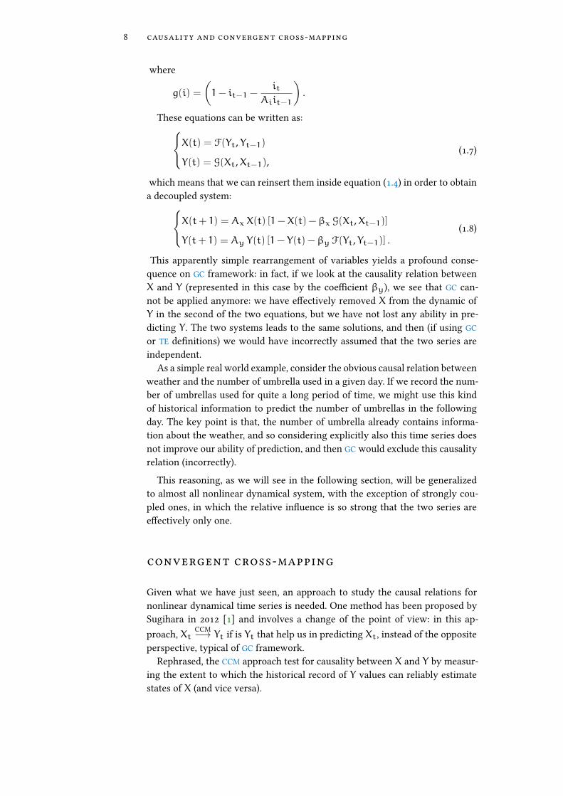
These equations can be written as:X(t) = F(Yt, Yt−1)
Y(t) = G(Xt,Xt−1),(1.7)
which means that we can reinsert them inside equation (1.4) in order to obtaina decoupled system:X(t+ 1) = Ax X(t) [1−X(t) −βx G(Xt,Xt−1)]
Y(t+ 1) = Ay Y(t) [1− Y(t) −βy F(Yt, Yt−1)] .(1.8)
This apparently simple rearrangement of variables yields a profound conse-quence on GC framework: in fact, if we look at the causality relation betweenX and Y (represented in this case by the coe�cient βy), we see that GC can-not be applied anymore: we have e�ectively removed X from the dynamic ofY in the second of the two equations, but we have not lost any ability in pre-dicting Y. The two systems leads to the same solutions, and then (if using GCor TE de�nitions) we would have incorrectly assumed that the two series areindependent.
As a simple real world example, consider the obvious causal relation betweenweather and the number of umbrella used in a given day. If we record the num-ber of umbrellas used for quite a long period of time, we might use this kindof historical information to predict the number of umbrellas in the followingday. The key point is that, the number of umbrella already contains informa-tion about the weather, and so considering explicitly also this time series doesnot improve our ability of prediction, and then GC would exclude this causalityrelation (incorrectly).
This reasoning, as we will see in the following section, will be generalizedto almost all nonlinear dynamical system, with the exception of strongly cou-pled ones, in which the relative in�uence is so strong that the two series aree�ectively only one.
convergent cross-mapping
Given what we have just seen, an approach to study the causal relations fornonlinear dynamical time series is needed. One method has been proposed bySugihara in 2012 [1] and involves a change of the point of view: in this ap-proach, Xt
CCM−→ Yt if is Yt that help us in predicting Xt, instead of the oppositeperspective, typical of GC framework.
Rephrased, the CCM approach test for causality between X and Y by measur-ing the extent to which the historical record of Y values can reliably estimatestates of X (and vice versa).
1.2 convergent cross-mapping 9
In order to understand why this can happen, we will need to introduce Tak-ens’ theorem, the main result of this chapter.
takens’ theorem and convergent cross-mapping
From a theoretical point of view, two time series are causally linked if they aregenerated from the coupled dynamical equations describing the evolution ofthe system under analysis.
For many dynamical system, there exist a subset of the phase space (calledattractor) that is the smallest that has the following properties:
• is forward invariant: if a point is inside the attractor, it will forever beinside;
• there exist a neighbor of this set (called basin of attraction) and the pointof this neighbors will eventually fall inside the attractor in the future.
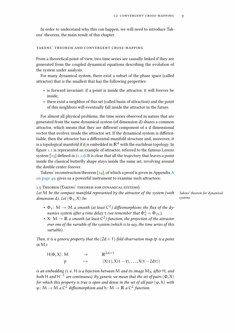
For almost all physical problems, the time series observed in nature that aregenerated from the same dynamical system (of dimension d) shares a commonattractor, which means that they are di�erent component of a d dimensionalvector that evolves inside the attractor set. If the dynamical system is di�eren-tiable, then the attractor has a di�erential manifold structure and, moreover, itis a topological manifold if it is embedded in Rd with the euclidean topology. In�gure 1.1 is represented an example of attractor, referred to the famous Lorenzsystem [23] de�ned in (1.12). It is clear that all the trajectory that leaves a pointinside the classical butter�y shape stays inside the same set, revolving aroundthe double center forever.
Takens’ reconstruction theorem [24], of which a proof is given in Appendix Aon page 49, gives us a powerful instrument to examine such attractors:
1.5 Theorem (Takens’ theorem for dynamical systems).LetM be the compact manifold represented by the attractor of the system (with Takens’ theorem for dynamical
systemsdimension d). Let (Φτ,X) be:
• Φτ : M → M a smooth (at least C2) di�eomorphism: the �ux of the dy-namics system after a time delay τ (we remember that Φ2τ = Φ2τ),
• X : M→ R a smooth (at least C2) function, the projection of the attractorover one of the variable of the system (which is to say, the time series of thisvariable).
Then, it is a generic property that the (2d+ 1)-fold observation map (p is a pointinM):
H[Φ,X] : M → R2d+1
p 7→ (X(t),X(t− τ), . . . ,X(t− 2dτ))
is an embedding ( i. e. H is a bijection betweenM and its imageMX after H, andbothH andH−1 are continuous). By generic we mean that the set of pairs (Φ,X)for which this property is true is open and dense in the set of all pair (ϕ,h) withϕ : M→M a C2 di�eomorphism and h : M→ R a C2 function.

10 causality and convergent cross-mapping
Figure 1.1: Schematic representation of the shadow manifolds obtained thanks to Takens’ recon-struction theorem.
What this theorem tells us is that, under certain mild hypotesis, we can �ndan exact (from a topological point of view) copy of the behaviour of the systemusing only one of the variables and his past history. This explains why in theprevious section we could manage to rearrange the coupled logistic system toexpress each variable only in term of itself and his past value.
Moreover, this allows us to make prediction: if we can reconstruct the dy-namic thanks to one variable, and our reconstruction is topologically equiva-lent, we can use the reconstructed attractor to predict the value of the othervariable.
Given a point p ∈ M of the attractor, we choose the variable X to obtainits projection in one coordinate and then, by means of Takens’ theorem, wecreate the di�eomorphic copy of the attractorMx, in which lives the copy px ∈Mx of the original point p. Takens’ theorem assure us that the topologies overthe two manifolds are homeomorphic, and thus the neighbors Up and Upx aredi�erentially the same, which means that to each point q ∈ Up correspondsone to one a point qi ∈ Upx .
convergent cross-mapping
We can then create a constructive method to obtain an estimate of one projec-tion from another one.
Let’s call the two series we are interested in X(t) and Y(t), the attractor man-ifold M of dimension d, E = 2d+ 1 the reconstruction dimension and τ thetime lag we are interested in (this will usually correspond to the lag betweentwo points in the time series, or a fraction of the period of the solution. Moreabout this choice will be told in Chapter 3).
1.6 Algorithm (Convergent Cross-Mapping).Algorithm for ConvergentCross-Mapping
• Choose a projection direction X.• Create the shadow manifold Mx by de�ning (for each t > E − 1) the
points X(t) = (X(t),X(t− τ), . . . ,X(t− τ(E− 1))).

1.2 convergent cross-mapping 11
• For each point Y(t), choose the corresponding X(t) and look for its E+ 1nearest neighborhood.
• Calling tk the time index of thekth-nearest neighborhood, calculate someweights wk based on the distances between X(tk) and X(t).
• Finally calculate Y(t) as a weighted sum
Y(t) =∑
k6E+1
wkY(tk).
As one can see, this algorithm provide an estimated time series Y(t) (exclud-ing the �rst E− 1 points for which we cannot create the shadow projection)that can be evaluated against the real Y(t), for example by calculating PearsonCorrelation Coe�cient (PCC) Pcc(Y, Y)3. We will call the correlation betweenY given X and Y as Pcc(X, Y), and usually we will use the parameter C(X, Y)de�ned as:
C(X, Y) = [Pcc(X, Y)]2 (1.9)
In order to calculate weights wk one should �nd a function that makes thenearest points more important: we want to give more importance to the nearestpoint, because they have a closer history. The function used by Sugihara is
wk =1
Wmax
(exp
[−‖Xk−Xt‖dmin
],wmin
)(1.10)
with W =∑kwk, Xk the kth-nearest neighborhood, dmin = ‖Xt − X0‖ the
distance between xt and its nearest neighborhood andwmin = 10−6 a securitythreshold for computational issues. If dmin = 0, it means that the nearest pointis actually superimposed to Xt, and then the sum is reduced to just that point(assigning all other weights to 0)
properties of convergent cross-mapping
CCM has many important property that can help us with our task of identifyingcausality. The �rst is the one that gives part of the name to the method:
Property 1.7 (Convergence): Calling L the lenght of the time series used to Cross-Map, Property of convergence ofCross-Mappingif the hypothesis of Takens’ theorem are satis�ed, Pcc[L] is a function that converge to 1
as L approaches in�nite, formally:
limL→∞ Pcc[L] = 1
3 PCC is de�ned for a population as
Pcc(X, Y) =Cov(X, Y)σXσY
.
For a sample xi and yi of size n this expression be rewritten in a more computationally conve-nient way as:
Pcc(X, Y) =n∑i xiyi −
∑i xi
∑i yi√
n∑i x2i − (
∑i xi)
2√n∑i y2i − (
∑i yi)
2

12 causality and convergent cross-mapping
Figure 1.2: The prediction ability for the cross-mapping between two time series in a prey-predator system, versus the length of the time series used to create the shadow man-ifold and make prediction. For each length an estimated series has been calculated,and the PCC with the corresponding true series has been calculated. The solid linerepresent the �t from Equation 1.11. The data comes from [25] and are freely avail-able at https://robjhyndman.com/tsdldata/data/veilleux.dat.
This property, exempli�ed in Figure 1.2, ensure us that, given a su�cientobservation time, each series will predict the others in the same attractor withperfect ability.
In order to test the quality of a prediction, then, one can explore how fast theestimated series converge to the measured one, for example by evaluating a �tof the data with an exponential law:
Pcc(L) = ρ0 −αe−γL (1.11)
where ρ0 should be as near to 1 as possible while γ is the speed of convergence.The fact that ρ0 is not always 1 is not unexpected nor a problem: the pres-
ence of noise (both due to the model and the measurement) hinder slightly thismethod, because as seen from Theorem 1.5 on page 9 we need the time �ux ofthe dynamics system to be C2, which cannot be said for a Stochastic Di�eren-tial Equation (SDE) in general4. Anyway, if the noise is su�ciently small, thisapproach works in the same way, but the prediction will not converge exactlyto the measured one.
Moreover, as I will discuss in Section 1.3 on page 15 and show in Chapter 2on page 17, the injection of a small quantity of noise will help the detection ofcausality relations.
Another important property which deserves to be mentioned is another di-rect consequence of the Taken’s theorem:
Property 1.8 (Choice of projection): The quality of the prediction depends on theProperty of the choice ofprojection projection chosen. Moreover, in certain cases, exists projections that cannot predict other
variables.
4 For some particular class of SDE an extension of Takens’ theorem has even been proven, see [26]
1.2 convergent cross-mapping 13
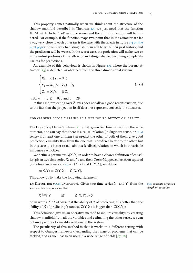
This property comes naturally when we think about the structure of theshadow manifold described in Theorem 1.5: we just need that the functionX : M → R to be "bad" in some sense, and the entire projection will be hin-dered. For example, if the function maps two point that in the attractor are faraway very close to each other (as is the case with the Z axis in �gure 1.3 on thenext page) the only way to distinguish them will be with their past history, andthe prediction will be worse. In the worst case, the projection will make two ormore entire portions of the attractor indistinguishable, becoming completelyuseless for predictions.
An example of this behaviour is shown in Figure 1.3, where the Lorenz at-tractor [23] is depicted, as obtained from the three dimensional system:
Xt = σ (Yt −Xt)
Yt = Xt (ρ−Zt) − Yt
Zt = XtYt −βZt.
(1.12)
with σ = 10, β = 8/3 and ρ = 28.In this case, projecting overZ-axes does not allow a good reconstruction, due
to the fact that the projection itself does not represent correctly the attractor.
convergent cross-mapping as a method to detect causality
The key concept from Sugihara [1] is that, given two time series from the sameattractor, one can say that there is a causal relation (in Sugihara sense, or CCMsense) if at least one of them can predict the other. If both of them give goodprediction, causality �ow from the one that is predicted better to the other, butin this case it is better to talk about a feedback relation, in which both variablein�uence each other.
We de�ne a parameter ∆(X, Y) in order to have a clearer de�nition of causal-ity: given two time seriesXt and Yt and their Cross-Mapped correlation squared(as de�ned in equation (1.9)) C(X, Y) and C(Y,X), we de�ne
∆(X, Y) = C(Y,X) −C(X, Y).
This allow us to make the following statement:
1.9 Definition (CCM causality). Given two time series Xt and Yt from the CCM causality de�nition(Sugihara causality)same attractor, we say that:
XCCM−→ Y i� ∆(X, Y) > 0,
or, in words, X CCM cause Y if the ability of Y of predicting X is better than theability of X of predicting Y (and so C(Y,X) is bigger than C(X, Y)).
This de�nition give us an operative method to inquire causality: by creatingshadow manifold from all the variables and estimating the other series, we canobtain a picture of causality relations in the system.
The peculiarity of this method is that it works in a di�erent setting withrespect to Granger framework, expanding the range of problems that can betackled, and as such has been used in a wide range of �elds [27, 28].
14 causality and convergent cross-mapping
X(t)
2015
105
05
1015
2025
Y(t)
30
20
10
0
10
20
30
40
Z(t)
0
10
20
30
40
50
60
(a) The attractor
0 200 400 600 800 1000
Lenght of Time Series [L]
0.2
0.0
0.2
0.4
0.6
0.8
1.0
Qualit
y o
f Pre
dic
tion [
PC
C]
x xmap y
x xmap z
y xmap x
y xmap z
z xmap x
z xmap y
(b) Correlations
Projection X
Projection Y
40 45 50 55 60 65 70
Time [s]
Projection Z
(c) Projections along the three axes
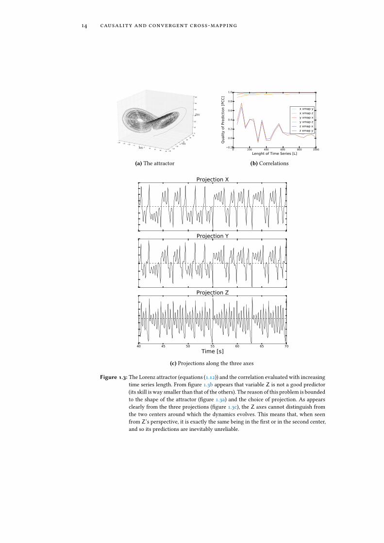
Figure 1.3: The Lorenz attractor (equations (1.12)) and the correlation evaluated with increasingtime series length. From �gure 1.3b appears that variable Z is not a good predictor(its skill is way smaller than that of the others). The reason of this problem is boundedto the shape of the attractor (�gure 1.3a) and the choice of projection. As appearsclearly from the three projections (�gure 1.3c), the Z axes cannot distinguish fromthe two centers around which the dynamics evolves. This means that, when seenfrom Z’s perspective, it is exactly the same being in the �rst or in the second center,and so its predictions are inevitably unreliable.

1.3 problem of convergent cross-mapping and extensions 15
problem of convergent cross-mapping and ex-tensions
Unfortunately, though, also this method presents some problems that can hin-der severely its applicability and that have been highlighted by McCracken etAl. in 2014 [12].
Mainly, the problem is that this method appears not to work in some rangeof parameters or for some particular systems, for which Taken’s hypotesis doesnot apply. More precisely, McCracken discusses two cases in particular: the �rstdi�culties appears when the system is strongly coupled. In this case, the strongcoupling allows for both projections to be equally good at predicting the timeseries evolution and the method fails in detecting causality. In some cases, thepresence of a strong coupling is evident from the data (for example if morethan one variable has the same, strong periodicity, probably one of them iscoupled strongly to the others and drives them) or is known from previousmeasurements or models. In those cases, probably Granger causality is a bettertest.
In the second case the method does not work depending on the shape of theattractor, and this is in generally di�cult to say even a posteriori! In this caseCCM may provide an unreliable result, but we do not have even a way to knowif we are actually in this situation or not. In other word there is not a systematicway to know if CCM is working or not. This problem has been addressed in [12],where some systems are investigated within a certain range of parameters andCCM appears to change its prediction.
This issue is closely related to the attractor manifold and the chosen projec-tion, and it is due to property 1.8 on page 12. In fact, if the attractor is shapedin such a way that one of the natural projection is not well suited for recon-struction (because it does not respect the hypotesis of Takens’ theorem), thencreating a reconstructed version of the attractor made with it will not be home-omorphic to the target one. This means that our prediction will become unreli-able, but if we are not aware that the problem is in the hypotesis of the theorem,we might think that this is a genuine e�ect of causality. For example, if we cal-culate ∆(X,Z) or ∆(Y,Z) for Lorenz attractor (see Figure 1.3 on the precedingpage) we �nd immediately that Z is strongly driven from both X and Y, whichis de�nitely not true. Obviously, in this example one could see this e�ect justby watching the trajectories, but other systems can be much more subtle.
A possible simple solution to this problem could be to change the projectionfunction, but of course this undermines the scope of the work, which is to un-derstand the relation between variables and not between function of variables.
pairwise asymmetric inference
In order to solve this problem, in [12] a variant to CCM method, called PairwiseAsymmetric Inference (PAI), has been proposed.
16 causality and convergent cross-mapping
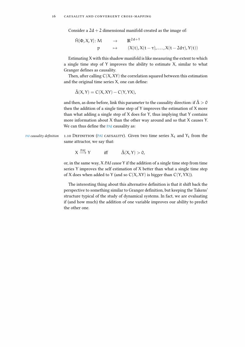
Consider a 2d+ 2 dimensional manifold created as the image of:
H[Φ,X, Y] : M → R2d+1
p 7→ (X(t),X(t− τ), . . . ,X(t− 2dτ), Y(t))
EstimatingXwith this shadow manifold is like measuring the extent to whicha single time step of Y improves the ability to estimate X, similar to whatGranger de�nes as causality.
Then, after callingC(X,XY) the correlation squared between this estimationand the original time series X, one can de�ne:
∆(X, Y) = C(X,XY) −C(Y, YX),
and then, as done before, link this parameter to the causality direction: if ∆ > 0then the addition of a single time step of Y improves the estimation of X morethan what adding a single step of X does for Y, thus implying that Y containsmore information about X than the other way around and so that X causes Y.We can thus de�ne the PAI causality as:
1.10 Definition (PAI causality). Given two time series Xt and Yt from thePAI causality de�nition
same attractor, we say that:
XPAI−→ Y i� ∆(X, Y) > 0,
or, in the same way, X PAI cause Y if the addition of a single time step from timeseries Y improves the self estimation of X better than what a single time stepof X does when added to Y (and so C(X,XY) is bigger than C(Y, YX)).
The interesting thing about this alternative de�nition is that it shift back theperspective to something similar to Granger de�nition, but keeping the Takens’structure typical of the study of dynamical systems. In fact, we are evaluatingif (and how much) the addition of one variable improves our ability to predictthe other one.

2A P P L I C AT I O N S O F C O N V E R G E N TC R O S S - M A P P I N G A L G O R I T H M O N AM O D E L E C O S Y S T E M
In order to test the CCM method and its limits, we apply it on times series gener-ated through a multi-species population dynamics model known as generalizedLotka-Volterra [29] (LV).
description of the system
The model is described in equations (2.1), where K is the carrying capacity forpreys (whose population is indicated by X), Y is the predators population and Edenotes state variable for the environment that is coupled with population dy-namics. The equations are stochastic as white noise [22] is added to the system.Three distinct sources of noise have been considered:
1. An environmental noise, additive for E, whose strength is identi�ed byits standard deviation σE;
2. Demographic (multiplicative white) noise in both predator and prey pop-ulation dynamics with intensity σX and σY , respectively;
3. A measurement noise, for both X and Y, mimicking uncertainties ob-tained by adding to the �nal series a white Gaussian noise with standarddeviation σMeas.
The most general formulation of this system is thus:E(t) = sinωt+ σEdW
Xt = aXt
(1− Xt
K
)− bXtYt + σXXtdW
Yt = (−c+ γE(t)) Yt + dXtYt + σYYtdW
(2.1)
where dW represents symoblically the in�nitesimal increments of a Wienerrandom walk processWt =
∫ξtdt with ξt = N(0, 1).
17
18 applications of convergent cross-mapping
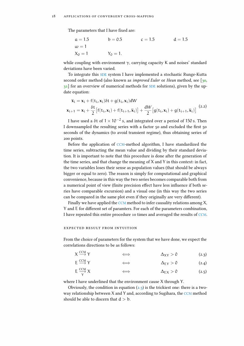
The parameters that I have �xed are:
a = 1.5 b = 0.5 c = 1.5 d = 1.5
ω = 1
X0 = 1 Y0 = 1.
while coupling with environment γ, carrying capacity K and noises’ standarddeviations have been varied.
To integrate this SDE system I have implemented a stochastic Runge-Kuttasecond order method (also known as improved Euler or Heun method, see [30,31] for an overview of numerical methods for SDE solutions), given by the up-date equation:
xi = xi + f(ti, xi)δt+ g(ti, xi)dW
xi+1 = xi +δt
2
[f(ti, xi) + f(ti+1, xi)
]+
dW2
[g(ti, xi) + g(ti+1, xi)
] (2.2)
I have used a δt of 1× 10⁻² s, and integrated over a period of 150 s. ThenI downsampled the resulting series with a factor 50 and excluded the �rst 50seconds of the dynamics (to avoid transient regime), thus obtaining series of200 points.
Before the application of CCM-method algorithm, I have standardized thetime series, subtracting the mean value and dividing by their standard devia-tion. It is important to note that this procedure is done after the generation ofthe time series, and that change the meaning of X and Y in this context: in fact,the two variables loses their sense as population values (that should be alwaysbigger or equal to zero). The reason is simply for computational and graphicalconvenience, because in this way the two series becomes comparable both froma numerical point of view (�nite precision e�ect have less in�uence if both se-ries have comparable excursion) and a visual one (in this way the two seriescan be compared in the same plot even if they originally are very di�erent).
Finally we have applied the CCM method to infer causality relations amongX,Y and E for di�erent set of paramters. For each of the parameters combination,I have repeated this entire procedure 10 times and averaged the results of CCM.
expected result from intuition
From the choice of parameters for the system that we have done, we expect thecorrelations directions to be as follows:
XCCM−→ Y ⇐⇒ ∆XY > 0 (2.3)
ECCM−→ Y ⇐⇒ ∆EY > 0 (2.4)
ECCM−→YX ⇐⇒ ∆EX > 0 (2.5)
where I have underlined that the environment cause X through Y.Obviously, the condition in equation (2.3) is the trickiest one: there is a two-
way relationship between X and Y and, according to Sugihara, the CCM methodshould be able to discern that d > b.
2.1 description of the system 19
0 20 40 60 80 100Time [s]
4
2
0
2
4
6
8
10
Abundance
[#
]
E(t)
X(t)
Y(t)
(a) K = 5
0 20 40 60 80 100Time [s]
1.0
0.5
0.0
0.5
1.0
1.5
2.0
2.5
3.0
Abundance
[#
]
E(t)
X(t)
Y(t)
(b) K = 500
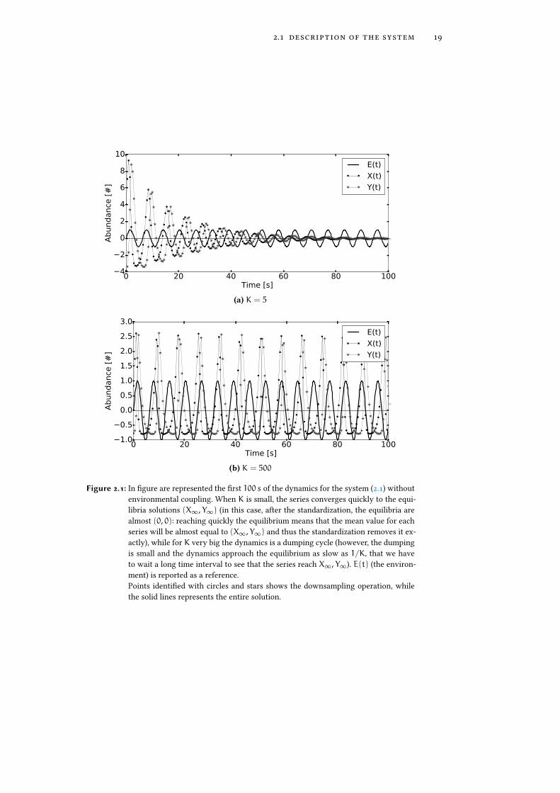
Figure 2.1: In �gure are represented the �rst 100 s of the dynamics for the system (2.1) withoutenvironmental coupling. When K is small, the series converges quickly to the equi-libria solutions (X∞, Y∞) (in this case, after the standardization, the equilibria arealmost (0, 0): reaching quickly the equilibrium means that the mean value for eachseries will be almost equal to (X∞, Y∞) and thus the standardization removes it ex-actly), while for K very big the dynamics is a dumping cycle (however, the dumpingis small and the dynamics approach the equilibrium as slow as 1/K, that we haveto wait a long time interval to see that the series reach X∞, Y∞). E(t) (the environ-ment) is reported as a reference.Points identi�ed with circles and stars shows the downsampling operation, whilethe solid lines represents the entire solution.
20 applications of convergent cross-mapping
Observing again system (2.1), we notice that when there is no coupling withenvironment, the system can be solved analytically by linearization of the equa-tions around the equilibria (X∞, Y∞), see Figure 2.1 on the preceding page. Theonly interesting equilibrium (in which neither of the variables goes extinct) isgiven by:
X∞ =c
d
Y∞ = −a(c− dk)
bdk.
The eigenvalues analysis of the linearized matrix shows that the two seriesin the phase space follow a spiral that falls to the equilibrium with a speed thatdepends (once �xed all the other parameters) on 1/K. Thus, in the case of asmall K the two series converge quickly to (X∞, Y∞), while if K is much biggerthat the other parameters, the equilibrium is reached after a long time.
Then, even if the second case is similar to an extended version of the transientregime of the �rst one, it allows us to explore what happens when there is anatural oscillation regime over the oscillations inducted by environment.
small carrying capacity
With a small carrying capacity (K = 5, we are in the situation depicted in�gure 2.1a on the previous page), the system quickly relaxes to (0, 0) (afterstandardization). If we exclude also the next 50 points, thus beginning measure-ments after 100 s, the attractor is a point (a manifold of dimension d = 0) andthen the hypothesis of Takens’ theorem are not applicable anymore, leading toa failure of CCM method. This fact is solved with the addition of model noise orwith a coupling with an external (driver) variable E(t).
effect of noise
The addition of model noise, most of the time, helps the detection of causality,even though it generally worsen the quality of prediction. In fact, thanks to thestochastic term, the solution deviates from (X∞, Y∞), and the dynamics can beobserved better. This is not the case for measurement noise, which does notmodify the dynamics nor the attractor shape.
In all this section I will focus on the e�ect of both kind of noise: for demo-graphic noise, I will vary Σ = σx = σy = σE in the interval [0, 0.5] with stepof 0.05, while σMeas ∈ {0, 0.1}.
Without environmental coupling (γ = 0)
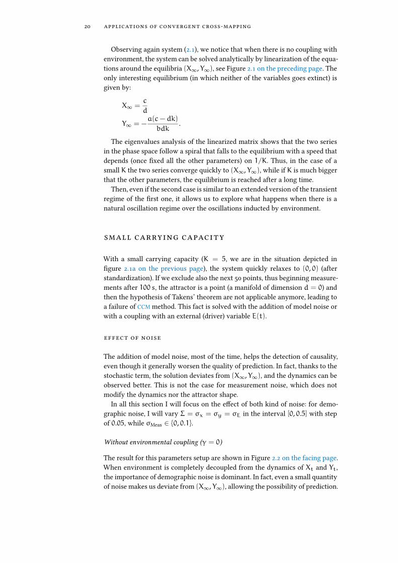
The result for this parameters setup are shown in Figure 2.2 on the facing page.When environment is completely decoupled from the dynamics of Xt and Yt,the importance of demographic noise is dominant. In fact, even a small quantityof noise makes us deviate from (X∞, Y∞), allowing the possibility of prediction.
2.2 small carrying capacity 21
0.0 0.1 0.2 0.3 0.4 0.5
Σ
0.0
0.2
0.4
0.6
0.8
1.0
C(I,J
)[Σ
]
C(E,X)
C(E,Y)
C(X,E)
C(X,Y)
C(Y,E)
C(Y,X)
(a) C(i, j)
0.0 0.1 0.2 0.3 0.4 0.5
Σ
0.2
0.1
0.0
0.1
0.2
0.3
0.4
0.5
∆(I,J
)[Σ
]
∆(E,X)
∆(E, Y)
∆(X, Y)
(b) ∆(i, j)
0.0 0.1 0.2 0.3 0.4 0.5
Σ
0.0
0.2
0.4
0.6
0.8
1.0
C(I,J
)[Σ
]
C(E,X)
C(E,Y)
C(X,E)
C(X,Y)
C(Y,E)
C(Y,X)
(c) C(i, j)
0.0 0.1 0.2 0.3 0.4 0.5
Σ
0.25
0.20
0.15
0.10
0.05
0.00
0.05
∆(I,J
)[Σ
]
∆(E,X)
∆(E, Y)
∆(X, Y)
(d) ∆(i, j)
Figure 2.2: Results for a system uncoupled from environment and with a small carrying capacity(K = 5). In �gures 2.2a and 2.2b the series have no measurement noise (which meansσMeas = 0), while �gures 2.2c and 2.2d refers to time series with σMeas = 0.1. Allplots are represented for the variation over Σ = σx = σy = σE, which grows from0 to 0.5.Di�erent markers identi�es couples of time series (Diamonds indicate the couple(X, Y), squares (E,X) and circles (E, Y)), while solid and dashed lines identify thetwo possible directions of the coupling: the solid line corresponds to i Predict−→ j, thedashed one with the same markers corresponds to j Predict−→ i.

22 applications of convergent cross-mapping
On the other hand, with no noise, because of the null dimensionality of theattractor space, the CCM fails.
From Figure 2.2a and 2.2c one can see the expected results: correlation be-tween series X and Y are moderately high (even if they decrease slightly withincreasing noise). As said before, the presence of a small demographic noise,when the prediction ability is severely hampered by measurement noise, helpde�nitely to predict something.
Interestingly, in Figure 2.2a, the �rst point (which has Σ = 0 = σMeas) showsa big prediction skill, even if there should be almost no dynamics at all. Thepoint is, from t = 50 s to approximately t = 100 s, the time series are notyet completely �xed in (X∞, Y∞) and they oscillate a little bit. In fact, all theprediction skill is based upon the �rst few points. This can be seen clearly if wemake CCM run only with points X(t), Y(t) with t > 100 s: the method doesnot work1.
The other interesting feature is that ∆(X, Y) 6 0, in contrast with what weexpect from condition (2.3), and the di�erence even increase by increasing Σor σMeas. This shows that CCM method can gives prediction which are againstintuition.
With strong environmental coupling (γ = 2)
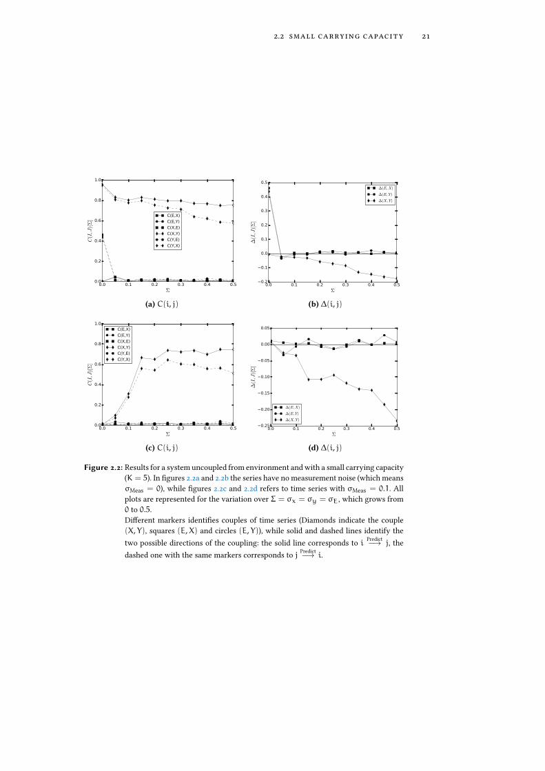
When we couple the system with environment by increasing the value of γ, we�nd some interesting results, shown in Figure 2.3.
First of all, now ∆(E,X) and ∆(E, Y) are signi�cantly bigger than zero, andalso show a certain hierarchy that is similar to what expected (since X is causedby E only through Y, we expect this causal relation to be weaker, or similarlythat E and X are worst in predicting each other).
Second, now for σMeas = 0we �nd∆(X, Y) > 0, which is more in accordancewith our expectations as expressed in equation (2.3).
effect of coupling with environment
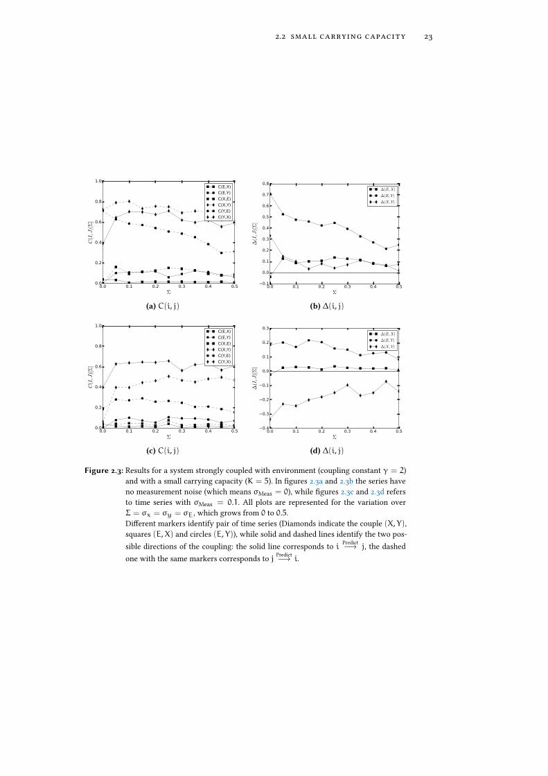
Let us consider now the e�ect of coupling with the external driver, variating γbetween 0 (no coupling at all) and 2 (quite big coupling), as shown in Figure 2.4.
The most interesting thing that appears from the plot of the correlation co-e�cient of �gures 2.4a, 2.4c is that increasing the coupling strength leads to adegradation of the prediction of the causality relation between the environmentand the system (for σMeas > 0.1. Even more interestingly, the sign of ∆(X, Y)changes (as clearly visible in �gure 2.4b) while increasing γ.
1 The problem does not come from CCM itself: predicting the evolution of something constant is,in fact, quite trivial. The point is that it is a meaningless problem and, moreover, PCC is not wellde�ned for two constant process.
2.2 small carrying capacity 23
0.0 0.1 0.2 0.3 0.4 0.5
Σ
0.0
0.2
0.4
0.6
0.8
1.0
C(I,J
)[Σ
]
C(E,X)
C(E,Y)
C(X,E)
C(X,Y)
C(Y,E)
C(Y,X)
(a) C(i, j)
0.0 0.1 0.2 0.3 0.4 0.5
Σ
0.1
0.0
0.1
0.2
0.3
0.4
0.5
0.6
0.7
0.8
∆(I,J
)[Σ
]
∆(E,X)
∆(E, Y)
∆(X, Y)
(b) ∆(i, j)
0.0 0.1 0.2 0.3 0.4 0.5
Σ
0.0
0.2
0.4
0.6
0.8
1.0
C(I,J
)[Σ
]
C(E,X)
C(E,Y)
C(X,E)
C(X,Y)
C(Y,E)
C(Y,X)
(c) C(i, j)
0.0 0.1 0.2 0.3 0.4 0.5
Σ
0.4
0.3
0.2
0.1
0.0
0.1
0.2
0.3
∆(I,J
)[Σ
]
∆(E,X)
∆(E, Y)
∆(X, Y)
(d) ∆(i, j)
Figure 2.3: Results for a system strongly coupled with environment (coupling constant γ = 2)and with a small carrying capacity (K = 5). In �gures 2.3a and 2.3b the series haveno measurement noise (which means σMeas = 0), while �gures 2.3c and 2.3d refersto time series with σMeas = 0.1. All plots are represented for the variation overΣ = σx = σy = σE, which grows from 0 to 0.5.Di�erent markers identify pair of time series (Diamonds indicate the couple (X, Y),squares (E,X) and circles (E, Y)), while solid and dashed lines identify the two pos-sible directions of the coupling: the solid line corresponds to i Predict−→ j, the dashedone with the same markers corresponds to j Predict−→ i.
24 applications of convergent cross-mapping
0.0 0.5 1.0 1.5 2.0
γ
0.0
0.2
0.4
0.6
0.8
1.0
C(I,J
)[γ]
C(E,X)
C(E,Y)
C(X,E)
C(X,Y)
C(Y,E)
C(Y,X)
(a) C(i, j)
0.0 0.5 1.0 1.5 2.0
γ
0.1
0.0
0.1
0.2
0.3
0.4
0.5
0.6
∆(I,J
)[γ]
∆(E,X)
∆(E, Y)
∆(X, Y)
(b) ∆(i, j)
0.0 0.5 1.0 1.5 2.0
γ
0.0
0.2
0.4
0.6
0.8
1.0
C(I,J
)[γ]
C(E,X)
C(E,Y)
C(X,E)
C(X,Y)
C(Y,E)
C(Y,X)
(c) C(i, j)
0.0 0.5 1.0 1.5 2.0
γ
0.2
0.0
0.2
0.4
0.6
∆(I,J
)[γ]
∆(E,X)
∆(E, Y)
∆(X, Y)
(d) ∆(i, j)
Figure 2.4: Results for a system with a small quantity of noise (Σ = 0.05) and a small carrying ca-pacity (K = 5). In �gures 2.4a and 2.4b the series have no measurement noise (whichmeans σMeas = 0), while �gures 2.4c and 2.4d refers to time series with σMeas = 0.1.All plots are represented for the variation over γ, which grows from 0 to 2.Di�erent markers identify pair of time series (Diamonds indicate the couple (X, Y),squares (E,X) and circles (E, Y)), while solid and dashed lines identify the two pos-sible directions of coupling: the solid line corresponds to i Predict−→ j, the dashed onewith the same markers corresponds to j Predict−→ i.
2.3 big carrying capacity 25
big carrying capacity
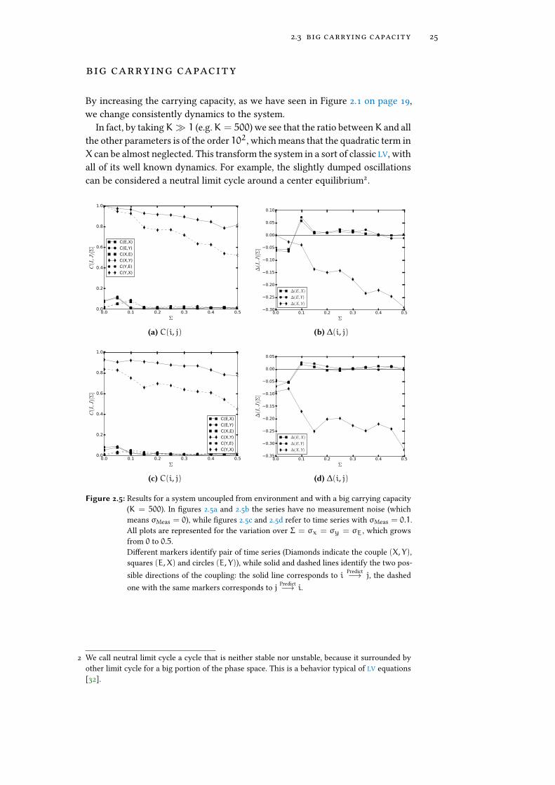
By increasing the carrying capacity, as we have seen in Figure 2.1 on page 19,we change consistently dynamics to the system.
In fact, by takingK� 1 (e.g.K = 500) we see that the ratio betweenK and allthe other parameters is of the order 102, which means that the quadratic term inX can be almost neglected. This transform the system in a sort of classic LV, withall of its well known dynamics. For example, the slightly dumped oscillationscan be considered a neutral limit cycle around a center equilibrium2.
0.0 0.1 0.2 0.3 0.4 0.5
Σ
0.0
0.2
0.4
0.6
0.8
1.0
C(I,J
)[Σ
]
C(E,X)
C(E,Y)
C(X,E)
C(X,Y)
C(Y,E)
C(Y,X)
(a) C(i, j)
0.0 0.1 0.2 0.3 0.4 0.5
Σ
0.30
0.25
0.20
0.15
0.10
0.05
0.00
0.05
0.10
∆(I,J
)[Σ
]
∆(E,X)
∆(E, Y)
∆(X, Y)
(b) ∆(i, j)
0.0 0.1 0.2 0.3 0.4 0.5
Σ
0.0
0.2
0.4
0.6
0.8
1.0
C(I,J
)[Σ
]
C(E,X)
C(E,Y)
C(X,E)
C(X,Y)
C(Y,E)
C(Y,X)
(c) C(i, j)
0.0 0.1 0.2 0.3 0.4 0.5
Σ
0.35
0.30
0.25
0.20
0.15
0.10
0.05
0.00
0.05
∆(I,J
)[Σ
]
∆(E,X)
∆(E, Y)
∆(X, Y)
(d) ∆(i, j)
Figure 2.5: Results for a system uncoupled from environment and with a big carrying capacity(K = 500). In �gures 2.5a and 2.5b the series have no measurement noise (whichmeans σMeas = 0), while �gures 2.5c and 2.5d refer to time series with σMeas = 0.1.All plots are represented for the variation over Σ = σx = σy = σE, which growsfrom 0 to 0.5.Di�erent markers identify pair of time series (Diamonds indicate the couple (X, Y),squares (E,X) and circles (E, Y)), while solid and dashed lines identify the two pos-sible directions of the coupling: the solid line corresponds to i Predict−→ j, the dashedone with the same markers corresponds to j Predict−→ i.
2 We call neutral limit cycle a cycle that is neither stable nor unstable, because it surrounded byother limit cycle for a big portion of the phase space. This is a behavior typical of LV equations[32].
26 applications of convergent cross-mapping
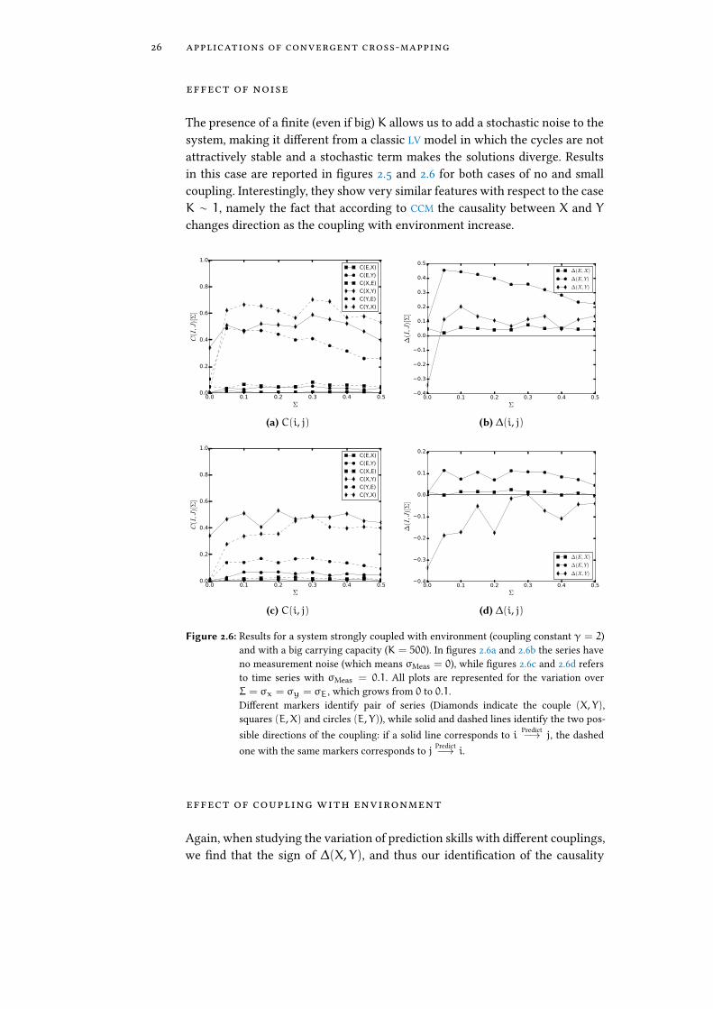
effect of noise
The presence of a �nite (even if big) K allows us to add a stochastic noise to thesystem, making it di�erent from a classic LV model in which the cycles are notattractively stable and a stochastic term makes the solutions diverge. Resultsin this case are reported in �gures 2.5 and 2.6 for both cases of no and smallcoupling. Interestingly, they show very similar features with respect to the caseK ∼ 1, namely the fact that according to CCM the causality between X and Ychanges direction as the coupling with environment increase.
0.0 0.1 0.2 0.3 0.4 0.5
Σ
0.0
0.2
0.4
0.6
0.8
1.0
C(I,J
)[Σ
]
C(E,X)
C(E,Y)
C(X,E)
C(X,Y)
C(Y,E)
C(Y,X)
(a) C(i, j)
0.0 0.1 0.2 0.3 0.4 0.5
Σ
0.4
0.3
0.2
0.1
0.0
0.1
0.2
0.3
0.4
0.5
∆(I,J
)[Σ
]
∆(E,X)
∆(E, Y)
∆(X, Y)
(b) ∆(i, j)
0.0 0.1 0.2 0.3 0.4 0.5
Σ
0.0
0.2
0.4
0.6
0.8
1.0
C(I,J
)[Σ
]
C(E,X)
C(E,Y)
C(X,E)
C(X,Y)
C(Y,E)
C(Y,X)
(c) C(i, j)
0.0 0.1 0.2 0.3 0.4 0.5
Σ
0.4
0.3
0.2
0.1
0.0
0.1
0.2
∆(I,J
)[Σ
]
∆(E,X)
∆(E, Y)
∆(X, Y)
(d) ∆(i, j)
Figure 2.6: Results for a system strongly coupled with environment (coupling constant γ = 2)and with a big carrying capacity (K = 500). In �gures 2.6a and 2.6b the series haveno measurement noise (which means σMeas = 0), while �gures 2.6c and 2.6d refersto time series with σMeas = 0.1. All plots are represented for the variation overΣ = σx = σy = σE, which grows from 0 to 0.1.Di�erent markers identify pair of series (Diamonds indicate the couple (X, Y),squares (E,X) and circles (E, Y)), while solid and dashed lines identify the two pos-sible directions of the coupling: if a solid line corresponds to i Predict−→ j, the dashedone with the same markers corresponds to j Predict−→ i.
effect of coupling with environment
Again, when studying the variation of prediction skills with di�erent couplings,we �nd that the sign of ∆(X, Y), and thus our identi�cation of the causality

2.4 summary 27
0.0 0.5 1.0 1.5 2.0
γ
0.0
0.2
0.4
0.6
0.8
1.0
C(I,J
)[γ]
C(E,X)
C(E,Y)
C(X,E)
C(X,Y)
C(Y,E)
C(Y,X)
(a) C(i, j)
0.0 0.5 1.0 1.5 2.0
γ
0.2
0.1
0.0
0.1
0.2
0.3
0.4
0.5
∆(I,J
)[γ]
∆(E,X)
∆(E, Y)
∆(X, Y)
(b) ∆(i, j)
0.0 0.5 1.0 1.5 2.0
γ
0.0
0.2
0.4
0.6
0.8
1.0
C(I,J
)[γ]
C(E,X)
C(E,Y)
C(X,E)
C(X,Y)
C(Y,E)
C(Y,X)
(c) C(i, j)
0.0 0.5 1.0 1.5 2.0
γ
0.4
0.3
0.2
0.1
0.0
0.1
0.2
0.3
0.4
∆(I,J
)[γ]
∆(E,X)
∆(E, Y)
∆(X, Y)
(d) ∆(i, j)
Figure 2.7: Results for a system with a small quantity of noise (Σ = 0.05) and a big carryingcapacity (K = 500). In �gures 2.4a and 2.4b the series have no measurement noise(which means σMeas = 0), while �gures 2.4c and 2.4d refers to time series withσMeas = 0.1. All plots are represented for the variation over γ, which grows from 0
to 2.Di�erent markers identi�es couples of series (Diamonds indicate the couple (X, Y),squares (E,X) and circles (E, Y)), while solid and dashed lines identify the two pos-sible directions of the coupling: the solid line corresponds to i Predict−→ j, the dashedone with the same markers corresponds to j Predict−→ i.
direction, depends on the variation of γ. In fact, as can be seen by �gure 2.7,when γ changes from γ 6 1 to γ > 1 the sign of ∆(X, Y) changes.
Again, the other interesting thing is that prediction ability decrease with theincreasing of γ, while the relation E CCM−→ X almost cannot be detected.
summary
The key of this example is that, by changing a parameter not directly linked tothe coupling X ↔ Y, one obtains opposite prediction from CCM method. Then,one can be in a di�cult position when trying to make detection of causality,depending on the exact dynamics of the system.
In fact, as we have seen, results obtained from CCM method applied to system(2.1) show some peculiarity that we already expressed in section 1.3: CCM e�ec-tiveness in detecting causal relationship does depend on the system parameters,
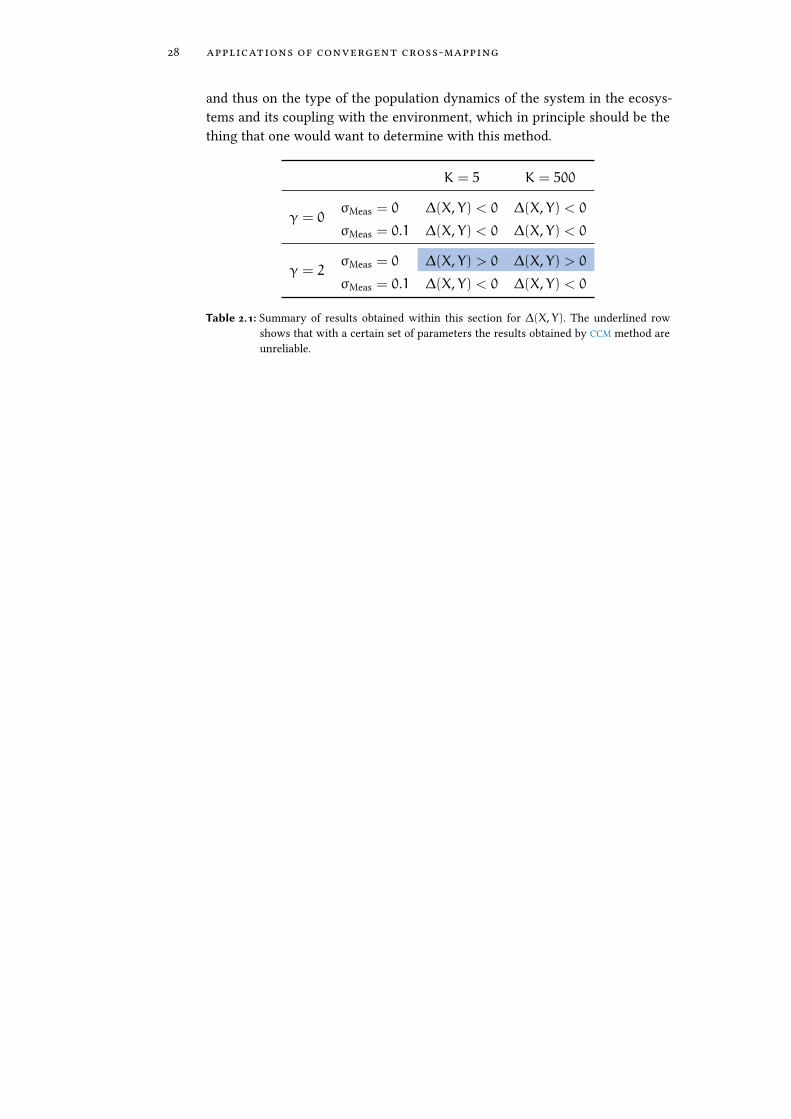
28 applications of convergent cross-mapping
and thus on the type of the population dynamics of the system in the ecosys-tems and its coupling with the environment, which in principle should be thething that one would want to determine with this method.
K = 5 K = 500
γ = 0σMeas = 0 ∆(X, Y) < 0 ∆(X, Y) < 0
σMeas = 0.1 ∆(X, Y) < 0 ∆(X, Y) < 0
γ = 2σMeas = 0 ∆(X, Y) > 0 ∆(X, Y) > 0
σMeas = 0.1 ∆(X, Y) < 0 ∆(X, Y) < 0
Table 2.1: Summary of results obtained within this section for ∆(X, Y). The underlined rowshows that with a certain set of parameters the results obtained by CCM method areunreliable.
3T H E M E T H O D O F A N A L O G S A N DT H E C U R S E O F D I M E N S I O N A L I T Y :I S P R E D I C T I O N P O S S I B L E ?
In most cases and for many complex systems (�nance, brain activity, earth-quakes, etc. . . ) we do not know the equations describing their evolution, or evenif we know them in theory, they cannot be computed exactly even with the mostpowerful of the super computer (e.g. whether forecast). However, if the systemdynamics is regulated by deterministic (even if unknown) laws, and if we know,through data, the past history of the system for enough time, can we predict itsfuture evolution?
In this chapter we present the method of analog, �rst introduced by Lorenzin 1969, and that tries to answer to this fundamental question. Two main exten-sions of this method exist, and will be also presented. The concept on which themethod is based is simple, and relies in the deterministic approach that Fromthe same antecedent follows the same consequent [3]: it is thus su�cient to �nda similar enough antecedent to make prediction about the consequent. Thisfundamental approach has been criticized already in XIX century by Maxwellstating [33]: It is a metaphysical doctrine that from the same antecedents followthe same consequents. [. . . ] But it is not of much use in a world like this, in whichthe same antecedents never again concur, and nothing ever happens twice. [. . . ]The physical axiom which has a somewhat similar aspect is that from like an-tecedents follow like consequents. In fact, Maxwell genius foresaw what now iswell known from chaos theory: the ubiquitous presence of irregular evolutionsdue to deterministic chaos.
Nevertheless, we are now in the era of Big Data and there is a growing opti-mism that what could not have been achieved in the past, it is now possible ande�ective [34]. As Chris Anderson, former editor-in-chief at Wired magazine,stated in a provocative way: This is a world where massive amounts of data andapplied mathematics replace every other tool that might be brought to bear. Outwith every theory of human behaviour, from linguistics to sociology. Forget tax-onomy, ontology, and psychology. Who knows why people do what they do? Thepoint is they do it, and we can track and measure it with unprecedented �delity.With enough data, the numbers speak for themselves. So, it is possible, if we haveenough data, to e�ectively predict the dynamics of complex system? Can the
29
30 method of analogs and dimensionality
method of analogs be successfully applied on a di�erent range of disciplinesopening up new perspective in the predictive analytics?
Following a recent work of a group of Italian physicists [3] we will show thatunfortunately the optimism must be limited: in fact there is an intrinsic limita-tion of the method that lies in the curse of dimensionality: if the system dimen-sionality is very large (and typically is), then the applicability of the method isspoiled, even using the largest data set available today.
method of analogs
The concept of the method of analogs, as said, is very straightforward in itsintuitive formulation and can be expressed as If a system behaves in a certainway, it will do so again, in agreement with a strict deterministic view of theworld.
In order to present the method of analogs, as introduced by Lorenz [35, 36]in its mathematical formulation, I will begin with a few notation.
Assume that xt describes the time series of a particular state of a complexsystem (e.g. the expression activity of di�erent genes at time t). Suppose thatwe have collectedN samples xk with k = 1, . . . ,N and that we want to forecastwhat state the system will assume in the future, that is to say that we want topredict the value of xN+τ.
The original idea is to search for a state among x1, . . . , xN−1, let us call it xk,that is the most similar to xN, and then use its consequents as proxies for theevolution of xN. Formally, calling ε-analog the nearest point to xN for whichholds ‖xk − xN‖ 6 ε, the prediction after τ time units is then:
xN+τ = xk+τ.
The �rst, simple, generalization is the so called Center of Mass (COM) predic-tion, where we consider for our estimate all the ε-analogs of xN, which meansall the n points xki , i = 1, . . . n, for which holds ‖xN − xki‖ 6 ε. From thisset of points, we determine the evolution of its center of mass, which is theweighted average of the analogs:
xN+τ =∑i
Wixki+τ,
where W is a suitable weight matrix, that in the simplest version of the methodis taken to be simply the n dimensional identity matrix or a more re�ned ex-pression such as the one in equation (1.10).
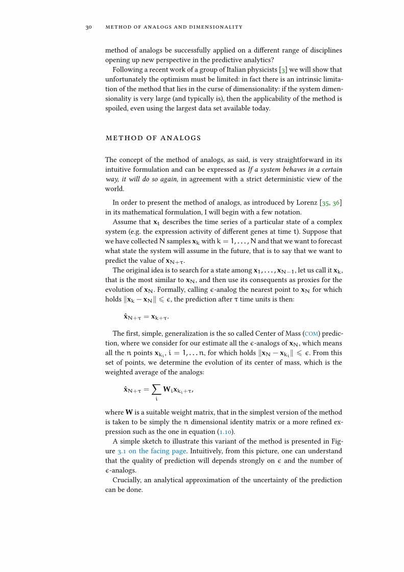
A simple sketch to illustrate this variant of the method is presented in Fig-ure 3.1 on the facing page. Intuitively, from this picture, one can understandthat the quality of prediction will depends strongly on ε and the number ofε-analogs.
Crucially, an analytical approximation of the uncertainty of the predictioncan be done.
3.1 method of analogs 31
Figure 3.1: Sketch of the method of analogs, where ε is the neighborhood dimension, Xkiis the
ith ε-analog and XN+τ is the estimate of future point.
In order to calculate the accuracy of prediction ‖xN+τ − xN+τ‖, one has toestimate xN+τ. Assuming that at least one good analog has been found, thenthe ε-analog xk can be assumed as a proxy of the present state xN, with anuncertainty δ0 set apart, i.e. xk = xN + δ0, where δ0 6 ε.
Then, we can express the expansion of this uncertainty over time with theMaximal Lyapunov Exponent (MLE)1, using the same approach of the discus-sions about sensitivity to initial conditions typical of chaotic dynamical systems:
δτ ' δ0eλτ, (3.1)
therefore, by de�ning∆ as the maximal tolerance about the error on prediction,we �nd that our estimated state will be ∆-accurate up to a time:
τ(δ0,∆) ≈ 1λ
ln∆
δ0, (3.2)
i.e. the time of prediction scales logarithmically with ∆/δ0.We thus have xN+τ = xk+τ+ δτ and substituting Eq. (3.1) the relative error
of the prediction is approximated by
‖xN+τ − xN+τ‖xN+τ
≈ ‖xk+τ(1+ δ0eλτ)‖
xk+τ∝ δ0eλτ, (3.3)
and because the MLE is �xed by the dynamic of the system, the only way toimprove the prediction is to minimize δ0.
The other (less natural) extension to Lorenz’s version of the method of analogsis called Local Linear (LL) prediction. As with all the methods in the analogmethod framework, also for LL predictor one �nds the k ε-analogs of the pointxN. Then, instead of taking the (weighted) average of the successors of theanalogs to estimate the successor of xN, the predictor is obtained by �tting alinear map L to the set of ε-analogs xi such that it minimize the di�erencebetween L(xi) and xi+τ, and then applying this map to the point xN.
1 We recall that the Lyapunov exponents describe the behavior of vectors in the tangent spaceof the phase space, and thus characterize the rate of separation of two points in�nitesimallyclose in the phase space. The importance of the MLE follows directly from the fact that this rateis exponential δt ∼ eλt and thus (if it is positive) the relevance of the bigger exponent willobliterate all the other. For a more accurate introduction to Lyapunov exponents see [37].

32 method of analogs and dimensionality
Even if this procedure is more re�ned than the COM approach, it is less intu-itive and presents the same problem (namely the search for nearest neighbors)of the simpler methods, and as such will not be discussed further.
takens’ embedding theorem and its applicationto the method of analogs
In the above presented explanation of the method of analogs, we have consid-ered x as a faithful representation of a given state of the system, and as such it isconsidered to be a point of the d-dimensional phase space (x ∈ Rd) measuredwith arbitrary precision.
Obviously, this is far from the reality of experiments, where measurementshave some noise determined by the experimental setup. Moreover, we can oftenmeasure only one or a few scalar variables linked to the real state of the systemthrough some unknown projection function. In other words we actually do notknow the phase space of the system.
Nevertheless, we can use Takens’ embedding theorem 1.5 on page 9 or itsextensions2 in order to reconstruct the phase space and then apply the methodof analog on this reconstructed space to make predictions.
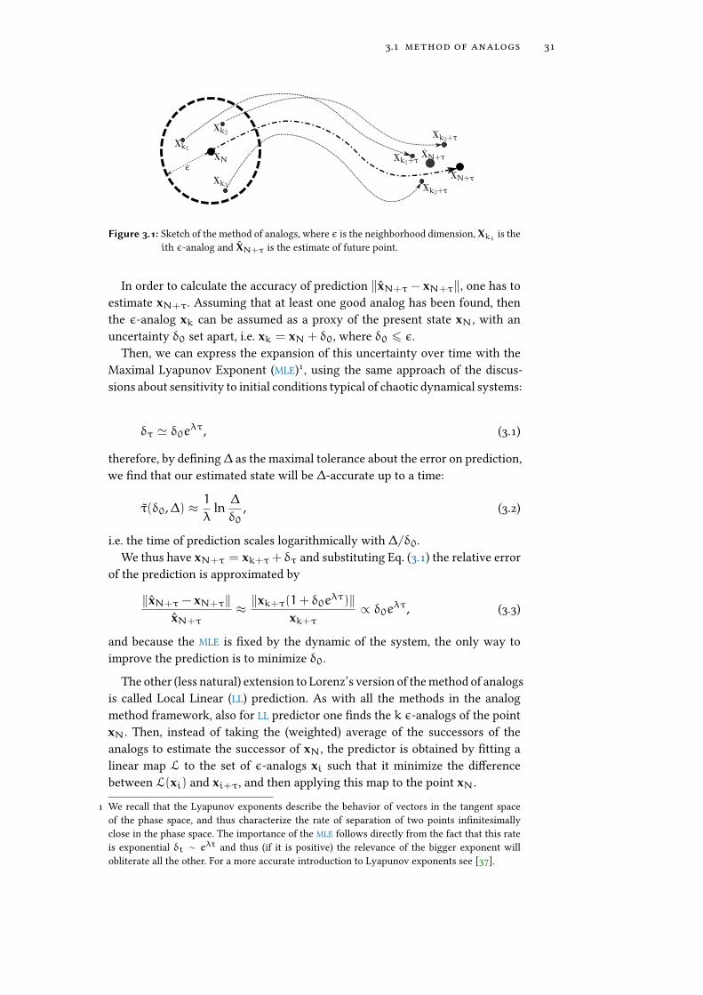
In Figure 3.2 an example of this approach is shown, applied to a �rst-di�erencetime series obtained from the tent map [40]:
xt+1 =
µxt xt <12
µ (1− xt) xt > 12 .
(3.4)
In particular, we have studied the case µ = 2, which is interesting becausethe generated time series has an autocorrelation function that goes to zero sorapidly that the series is indistinguishable (with this approach) from a purewhite random sequence. In this example, the embedding dimension used isE = 3, which is more than enough to display the complete dynamics of theattractor (which has an attractor dimension 0.97± 0.03 [41], determined withthe Grassberger approach, see section 3.3), and a time lag τ = 1. As Figure 3.2bshows, the prediction ability steeply decreases after few time steps in the future,a symptom of the chaotic nonlinear dynamics (and the Lyapunov divergence oforbits, equation (3.1)).
The reconstruction of the phase space is one of the main procedure usedwhen dealing with chaotic dynamical series, also because often just a simplevisual inspection of the data in the embedding space allows some understand-ing of the system. This approach, though, does not overcome nor mitigate theproblems that will be examined in the later sections.
2 For example, if the attractor has a fractal dimension, Takens’ theorem cannot be applied butits extension by Sauer et Al. [38] called Fractal Delay Embedding Prevalence Theorem still holds.Other notable extensions are proved in [26, 39] and generalize the theorem to some stochasticequations.
3.2 takens’ theorem and prediction 33
-1
-0.8
-0.6
-0.4
-0.2
0
0.2
0.4
0.6
0 100 200 300 400 500 600 700 800 900 1000
Delta
(t)
Time [s]
(a) ∆t
1 2 3 4 5 6 7 8 9 100.0
0.2
0.4
0.6
0.8
1.0
(b) Pcc(∆t, ∆t) vs TP
Figure 3.2: In �gure 3.2a are shown 1000 points of a time series obtained as ∆t = xt+1 − xtwhere xt is generated from the tent map (3.4). The �rst 500 points of the series areused to construct the training attractor (with E = 3 and τ = 1), and then predictionTp step in the future are made for each of the next 500 points (excluding the last Tppoints for which we don’t have a "measured" version Tp step in the future). In �gure3.2b is shown the PCC between the predicted points and the real ones as a functionof the number of step in the future we want to predict.
delay reconstruction and the problem of finding a good em-bedding
In this section, I will explain some details of Takens approach to the method ofanalogs following [42, § 3, 9].
Suppose that the only measure that we have access to is a scalar which is afunction of the (unknown) state vector x:
un = h (x(nδt)) + ηn
with h : M→ R some unknown scalar projection and ηn some white randommeasurement noise. We can then de�ne the vector:
un =(un,un−τ,un−2τ, . . . ,un−(m−1)τ
)(3.5)
where τ is the lag andm is the embedding dimension. In order to ful�ll the delayembedding theorem requirements, the choice ofmmust be done in accordanceto a strict criterion, while the choice of τ is more free, even if some particularvalues are better than others.
Choice of the embedding dimension
The choice of m is �xed by Takens’ theorem and its extensions, and must besuch that:
m > 2DM
whereDM is the dimension of the subsetM, called attractor, of the (unknown)phase space in which the orbits of the system are bounded. If DM is non in-teger, M is said to be a fractal attractor and this condition says that m must

34 method of analogs and dimensionality
be strictly larger than twice DM, while if DM is an integer we get back thefamiliar Takens’ claim thatm = 2DM + 1.
The problem is that most of the time we have no idea of the attractor dimen-sion, and we may even do not know if an attractor exist at all (that is to say, wedon’t know if the system is regulated by a (non)linear deterministic dynamicsor if it is driven solely by a stochastic process).
Of course, if we choose a very high m, bigger than the truem, we will obtaina correct embedding anyway, so one can be tempted to just set a very high mand use that to make prediction. This approach, thus, leads to two non trivialproblems: one is linked to the number of analog within radius ε (and will beaddressed in the next section), while the other is more theoretical and linked tothe MLE: the larger ism, the more far in the past will be the last component of u,which will be at a lagmτ. This implies that our algorithm for prediction is pro-cessing (with the same weight) information that we know are almost unrelatedwith the point of interest.
One of the most useful method to choose m is the so called method of Falsenearest neighbours [43].
Let m be the real but unknown embedding dimension, and let m < m bethe dimension in which, using the available data, we perform the embeddinginstead. The map that transform points from m to m is a projection in whichsome of the axes are eliminated (precisely m−m axes are eliminated). Thus,points that are separated with a large distance along one axes that is deleted bythe projection appears, in the m-dimensional space, as neighbors even if theyare not so (in this sense the method is called of false neighbors).
If we call
dmi =∥∥∥u(m)i − u(m)
k(i)
∥∥∥Max
the distance (inm dimensions) between ui and its nearest neighbors k(i)withinthe maximum norm, we can express the fraction of false neighbors going fromdimensionm tom+ 1 as:
χ(m)fnn (r) =
1
N
N∑i=1
Θ(dm+1i
dmi− r)
, (3.6)
where Θ(•) is the Heaviside step function that counts the couple for which theratio between their distance inm+ 1 andm dimension is bigger than a certainthreshold r.
A visual explanation of this approach is represented in Figure ??.A correction to this method, proposed by Hegger and Kantz [44], to account
for noise in the data (which keep the number of false neighbours steady be-cause the embedding dimension of a random process is in�nite) is to considerin Equation 3.6 only those points having a distance inm dimension
dmi <σ
r,
where we have de�ned σ to be the standard deviation of data. This correctiontakes into account the simple but important fact that two points cannot be false
3.2 takens’ theorem and prediction 35
0.0001
0.001
0.01
0.1
1
0 2 4 6 8 10 12 14 16
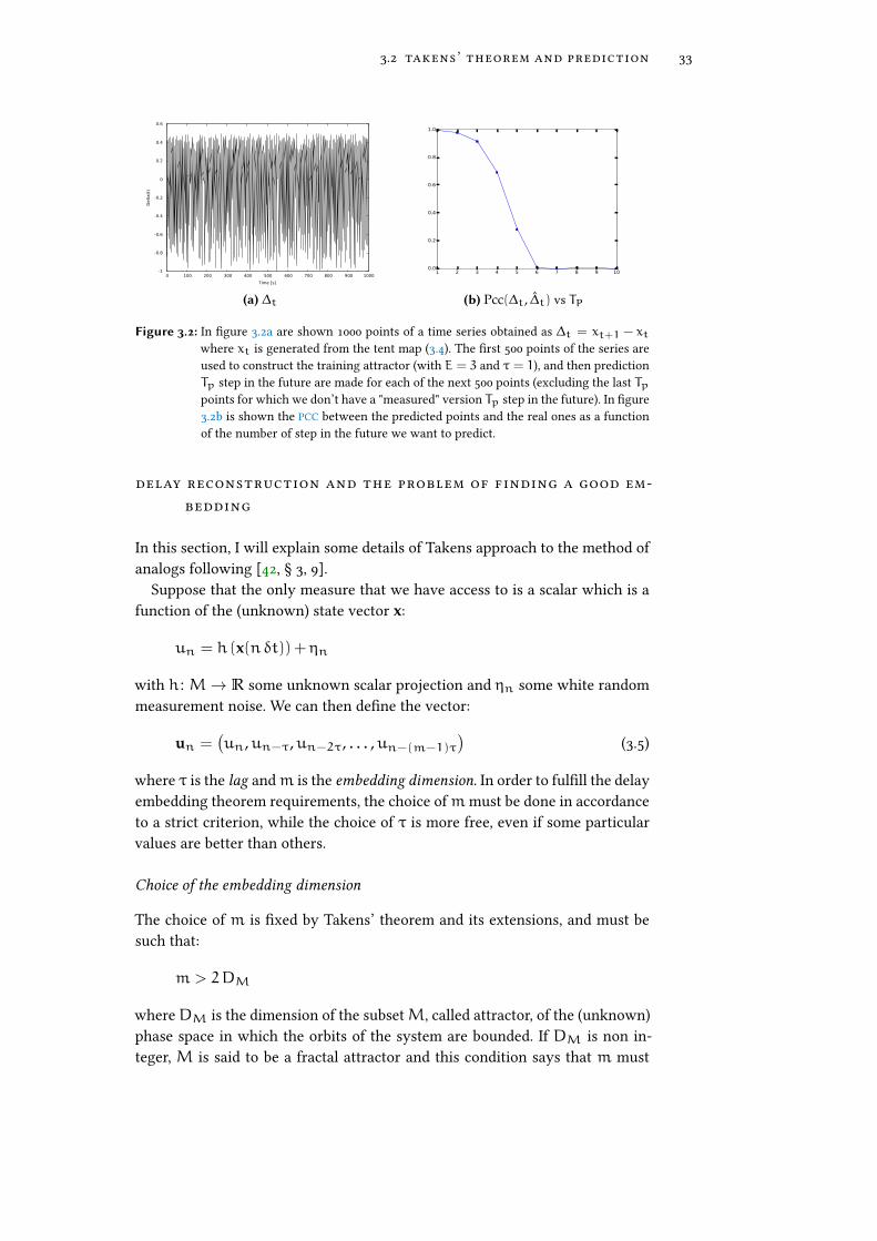
M = 1M = 2M = 3M = 4M = 5M = 6
Figure 3.3: Method of the False Nearest Neighbors for the Lorenz attractor. Each line representsa di�erent embedding dimensionM. As can be seen, passing from dimensionM = 4
to dimensionM = 5 there is a sharp increase in the steepness of the curve describingthe number of false neighbors as a function of the ratio of the distance in the twodimensions, suggesting that M = 5 is the correct embedding dimension. This isin agreement with the known correlation dimension of Lorenz attractor, which isslightly above two (DA ' 2.04), leading to an embedding dimension M > 2DA '4.
neighbors if already in m dimension their distance is larger than the standarddeviation times 1/r (on average they cannot be at a distance larger than σ).
Choice of time lag
The other free parameter in the delay embedding approach is the time lag τ,which presents a further di�culty: in fact, even though theoretically this pa-rameters does not have an importance in the phase space reconstruction (it doesnot appear in the formulations of Takens’ theorems nor in its extension), from apractical point of view choosing the right τ has some important consequencesin the ability to resolve the attractor and then to make e�ective prediction.
In fact, if τ is too short with respect to the characteristic time of the systemdynamics (such as the main period, if it exists), successive coordinates of thedelay vectors are strongly correlated, and all the points ui tend to places them-selves around the diagonal of Rm.
Instead, if τ is chosen to be too large, the ui points are almost completelyuncorrelated and they �lls a very large cloud of Rm, becoming non informative.
There are two main statistical approaches to this problem, based on the au-tocorrelation function and on the mutual information, respectively.
The �rst one is a minimalist approach, and it is based upon the idea that tomaximize the amount of information by extracting pair of points, they haveto be uncorrelated. Then, the best choice τ0 would be the delay that gives the
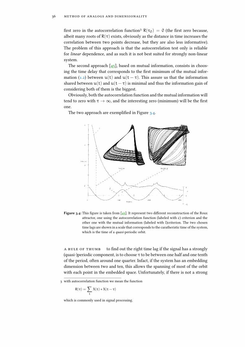
36 method of analogs and dimensionality
�rst zero in the autocorrelation function3 R(τ0) = 0 (the �rst zero because,albeit many roots of R(τ) exists, obviously as the distance in time increases thecorrelation between two points decrease, but they are also less informative).The problem of this approach is that the autocorrelation test only is reliablefor linear dependence, and as such it is not best suited for strongly non-linearsystem.
The second approach [45], based on mutual information, consists in choos-ing the time delay that corresponds to the �rst minimum of the mutual infor-mation (1.2) between u(t) and u(t − τ). This assure us that the informationshared between u(t) and u(t− τ) is minimal and thus the information gain ofconsidering both of them is the biggest.
Obviously, both the autocorrelation function and the mutual information willtend to zero with τ → ∞, and the interesting zero (minimum) will be the �rstone.
The two approach are exempli�ed in Figure 3.4.
Figure 3.4: This �gure is taken from [45]. It represent two di�erent reconstruction of the Rouxattractor, one using the autocorrelation function (labeled with c) criterion and theother one with the mutual information (labeled with I)criterion. The two chosentime lags are shown in a scale that corresponds to the caratheristic time of the system,which is the time of a quasi-periodic orbit.
a rule of thumb to �nd out the right time lag if the signal has a strongly(quasi-)periodic component, is to choose τ to be between one half and one tenthof the period, often around one quarter. Infact, if the system has an embeddingdimension between two and ten, this allows the spanning of most of the orbitwith each point in the embedded space. Unfortunately, if there is not a strong
3 with autocorrelation function we mean the function
R(τ) =∑t
X(t) ∗X(t− τ)
which is commonly used in signal processing.

3.3 statistical difficulty in method of analogs 37
periodic component or if the system is very large, this reasoning cannot beapplied.
the curse of dimensionality: statistical diffi-culties for good analogs and kac’s lemma
The accuracy estimation of the prediction given by (3.3) highlights how analogsthat are distant δ0 from the state xN will give exponentially distant far predic-tion from the "real" one as a function of the future time. This result remindsto the typical problem of sensitivity to initial conditions in dynamical systemswith chaotic behaviour: the same dynamics with initial condition that are dif-ferent of a little amount δ0 will give exponentially (with time) far trajectories[37].
However, if we look deeply in Eq. (3.3) things are di�erent in the two cases. Infact, as shown in the work of Cecconi et Al. [3], the main issue in Eqs. (3.3) and(3.2) is �nding good analogs, which means �nding points ε-near to the currentstate with a su�ciently small ε that allows τ to be large enough so that we canactual make future predictions within a maximal tolerance in the error of theprediction (∆).
However, as we will see in the next section, because of the curse of dimen-sionality the amount of data needed to obtain a good analogs increases expo-nentially with the system size.
dimensionality and degrees of freedom
The theory of ergodic dynamical systems is founded upon the principle thatlong-term statistical properties of a system can be described with the time-independent probability distribution µ(σ) of �nding the system in any speci�cregionσ of the phase space which, for a system withdDegrees of Freedom (DoF),is a region σ ⊂ Rd of the phase space.
If the evolution is conservative (as in Hamiltonian mechanics), it conservesvolumes in the phase space, then the probability dµ(x) of �nding the systemin a small region dV around x is proportional to the measure of dV . Instead,in dissipative systems, volumes in the phase space are contracted (on average)until probability dµ(x) is concentrated in a subsetM ⊂ Rd of dimensionDMcalled attractor. DM is thus what we call the system e�ective dimension, i. e.the dimension of the subspace of the phase space that is really spanned by thesystem.
Formally, the dimensionDM describes the small-scale behavior of µε of �nd-ing points x ∈ M inside the d-dimensional sphere Bdy (ε) of radius ε and cen-tered around y:
µ(Bdy (ε)
)=
∫Bdy (ε)
dµ(x) ∼ εDM (3.7)
38 method of analogs and dimensionality
Thus, in dissipative systems, trajectories of the system are e�ectively de-scribed by a number DM < d of DoF, even though they are de�ned in a d-dimensional space. If DM is non integer, the attractor is said to be fractal, andthis condition is typical for chaotic systems (consider for example [46])4.
In order to obtain an estimate ofDM, we follow the approach of Grassbergerand Procaccia [4], �rst de�ning the correlation sum as a function of the distanceε:
C(ε) ≡ limN→∞ 1
N2
N∑i,j=1
Θ(ε−
∥∥xi − xj∥∥) . (3.8)
This de�nition can be rewritten in term of the standard correlation function
c(r) =N∑i,j
[〈xi(0)xj(r)〉− 〈xi(0)〉 〈xj(r)〉
]as
C(ε) =
∫ε0
dr c(r) .
The key point proved by Grassberger and Procaccia is that this function be-haves as a power law of ε with an exponent ν when ε is su�ciently small:
C(ε) ∼ εν (3.9)
and that this exponent is an estimate of the system dimensionality, ν ∼ DM.In �gure 3.5 is represented the estimation of ν from the Correlation sum (3.8)using a simple counting algorithm. It is important to observe that the power lawscaling holds only for small ε, which will have consequences in the followingdiscussion. In order to understand intuitively the Grassberger-Procaccia claim,we see that the de�nition of correlation sum (3.8) can be thought as the fractionof ε-analogs of a certain point xk averaged over all the points xk of the timeseries.
Now we can see the analogy with ergodic theory: because (3.8) is an estimateof the averaged probability of �nding the system in a sphere of radius ε, byexploiting relations (3.7) and (3.9) we can derive:
εν ∼ C(ε) ≈ 〈µε〉 ∼ εDM =⇒ ν ≈ DM ≈ D.
In the following, I will use D as a uni�ed symbol for both ν andDM, neglectingthe small di�erence between the two.
The Grassberger-Procaccia exponent ν, which is called correlation dimension,is computationally (at least in principle) easy to compute: it is su�cient to cal-culate the function in the limit (3.8) for some value of ε and then �t the powerlaw (3.9).
Before explaining the reason of why this happens only in principle, I willintroduce the relation between correlation dimension and recurrence time (andPoincaré recurrence theorem).
4 In general, attractor are inhomogeneous inDM, and to di�erent Y corresponds di�erentDM. Inthis thesis we will ignore this technicality and study only attractor with a single fractal dimensionDM. For a more detailed discussion, that goes beyond the scope of this work, about multifractalattractor see [47]

3.3 statistical difficulty in method of analogs 39
−25
−20
−15
−10
−5
0
5
10
−6 −4 −2 0 2 4 6 8
ε-a
nalo
gra
tio[lo
g 2(C
)]
Radius of NN search (arbitrary scale) [log2(ε)]
C(ε)
ε2.05
Figure 3.5: Estimate of the correlation dimension ν from the correlation sum for the Lorenzattractor.
relation between correlation dimension and poincaré recur-rence theorem
We recall the classical result of Poincaré recurrence theorem [48], phrased in amathematical language that applies to our problem:
3.1 Theorem (Poincaré recurrence theorem).Lets call Φt the �ow of a volume-preserving di�erential system with bounded Poincaré recurrence theorem
orbit.Then, for each open set U of the phase space almost all the orbits Φt(x) with
x ∈ U, intersect U in�nitely many times, which means that there exists in�nitelymany τ such thatΦτ(x) ∈ U. Thus, the set of points x ∈ U for which this propertydoes not hold has zero measure.
Even if the theorem stresses that Φt must be volume-preserving, one canextend this result even to dissipative systems, provided that U ⊂ M, whichmeans that the only trajectories that return in�nitely many times are the onesthat start from the attractor.
Moreover, another straight extension is the one to ergodic systems, consider-ing the measure on the bounded phase space as the invariant probability µ(σ),then the points that does not return have zero probability. In this frameworkthe recurrence time τσ(x0) can be de�ned as the time that the trajectory that�ows from a point x0 needs in order to return inside the set σ that contains x0,which can be written as:
τσ(x0) = infk
{k > 1 | xk ∈ σ} δt. (3.10)
Averaging this time over all point in σ one obtains the average recurrencetime for points in σ:
〈τσ〉 =1
µ(σ)
∫σ
dµ(x) τσ(x) (3.11)
40 method of analogs and dimensionality
Now, we recall the classical Kac’s result [49] that states:
3.2 Theorem (Kac’s lemma).For an ergodic system, given σ ⊂M a non empty subset on the attractorM, µ(σ)Kac’s lemma
an invariant probability measure onM and τσ(x) de�ned as in equation (3.10),then: ∫
σ
dµ(x) τσ(x) = 1,
which means that, recalling equation (3.11), the average recurrence time is:
〈τσ〉 =1
µ(σ).
In other words, the average recurrence time to a region σ of the attractor is just theinverse of the probability of �nding the system in a state inside σ.
This result can be seen as one of the foundation principle of statistical me-chanics [3]: in fact, for a systems in Rd (and thus with d DoF) and with anaccessible volume Ld (which is the mean excursion of each component of x), ifthe phase space volumes is preserved and we consider σ as the hypercube oflinear dimension ε,then
µ(σ) ∼(εL
)d=⇒ 〈τσ〉 ∼
(L
ε
)d.
This means that the recurrence time grows exponentially with d, which meansthat for system of macroscopic size (where d is typical of the order ∼ 1023, forexample, but this holds even in much smaller system of around 103 particles)〈τσ〉 becomes enormous for any σ. This is the classical concept of irreversibilityas stated by Boltzmann himself (even without knowing Kac’s lemma) [50].
However this results also means that the chance of �nding good analogs de-crease exponentially with the dimension of the system.
conseqences on the method of analogs
Let’s consider a time series x1, . . . xk of points sampled at a time interval δt.We call K(ε) the number of ε-analog of the last point xk that have been foundin this series. Then, the average time between two such ε-analog of xk (whichgives us an estimate of the time needed to return ε-close to xk) is:
τk =(k− 1)δt
K(ε). (3.12)
Consider the correlation sum de�ned in equation (3.8), then we can implicitlyde�ne Ck(ε)
C(ε) =1
N
N∑k
Ck(ε)

3.3 statistical difficulty in method of analogs 41
that represents the fraction of ε-analog of the kth point of the series over thetotal data points N. Clearly, given this de�nition and equation (3.12)
Ck(ε) =K(ε)
k− 1=δt
τk. (3.13)
In order to make a∆-accurate estimate in predicting the last point xN throughthe past trajectoriy, we need at least N > τN. Recalling the scaling law (3.9)and using the relation (3.13), we prove that the number of points needed scalesas:
N ∼ ε−D, (3.14)
which is inversely proportional to the accuracy ε (as expected) but also expo-nential in D. This results highlights how for large systems (where the attractordimension can larger than 10) prediction becomes almost impossible at a rea-sonable ε.
Moreover, it states the precise limit of the Grassberger-Procaccia procedureto estimate the correlation dimension, given that the larger the correlation di-mension the larger is the number of points that are needed to sample the attrac-tor with a given accuracy ε, also considering that the scaling (3.9) holds in thelimit ε→ 0.
Of course one of the main challenge is to estimate both D and ε for realsystem, when only a set of time series are known.
For example, in one of his work, Smith [51] proposed an estimae of ε inorder to calculate the e�ective dimension D using the Grassberger-Procacciaalgorithm. In particular, he found that the minimum number of point that needsto be measured from the attractor (following the scaling law in equation (3.14))is
N ∼ 42D.
This means that for a D ' 5, N should be already of the order ∼ 108 toobtain a consistent estimate of the system relevant parameters.


4T H E C U R S E O F D I M E N S I O N A L I T Y , AN U M E R I C A L E X A M P L E
In this chapter I will provide some numerical example of the considerationsmade in chapter 3 on page 29, studying a simple system (the so called Lorenzattractor [23]).
description of the system: lorenz attractor in3 dimension
The �rst example is the classical three dimensional Lorenz attractor, that is de-scribed by
Xt = σ (Yt −Xt)
Yt = Xt (ρ−Zt) − Yt
Zt = XtYt −βZt.
(4.1)
with σ = 10, β = 8/3 and ρ = 28.In order to simulate this system I have implemented the same second order
Runge-Kutta method as in chapter 2 equation (2.2), using a time step δt = 0.01,which I then downsampled of a factor 50 in order to get a sampling frequencyof 2Hz.
For each time series, I have runned the algorithm ten times choosing randominitial condition inside the attractor basin, then averaging over the results inorder to avoid statistical coincidence.
grassberger-procaccia algorithm for the cor-relation dimension
The �rst algorithm that I have studied is the Grassberger-Procaccia algorithmto estimate the correlation dimension, which has been obtained by Grassbergerand Procaccia using a time series of 15 000 points [4] and is equal:
D = 2.05± 0.01. (4.2)
43

44 numerical approach to the curse of dimensionality
In Figure 4.1 the correlation dimension is estimated using time series of in-creasing length. It can be seen that the methods produces wrong results if thenumber of data is to small.
In fact, as shown in the previous chapter, the minimum number of points toget a reliable estimation of D is, according to Smith’s work [51],
Nmin = 42D ' 2125 points. (4.3)
−10
−8
−6
−4
−2
0
2
−3 −2 −1 0 1 2
ε2.7
ε2.0
47
103 data5 · 103 data105 dataCo
rrelationfunctio
n[lo
g(Cε)]
Distance [log(ε)]
Figure 4.1: Correlation function as calculated by the Grassberger-Procaccia algorithm [4], rep-resented in a log-log plot. The di�erent colors corresponds to di�erent length of theinput time series, and the lines represent the best �t obtained for the time series withone thousand points and the one with one hundred thousands points. The straightlines represents the best �tting power law C = aεD to two series of data (the short-est and the longest one). It can be noted that the points obtained with the series of5000 points follows almost exactly the line with D = 2.05.The solid range of the lines represents the range of data used for the �t.
The best result for the correlation dimension obtained �tting a power lawC = aεD is (using the time series with 100 000 points)
D105 = 2.047± 0.002 (4.4)
which is perfectly compatible with the values determined by Grassberger andProcaccia, in equation (4.2).
However, also calculating the �t with 5000 points yields a result compatiblewith the expected one:
D5·103 = 2.03± 0.02,
while the �t with 1000 points gives a wrong result as D103 = 2.67± 0.1.

4.2 center of mass prediction algorithm 45
Obviously, in order to make the �t, points with ε to large have been discarded,because the power law holds only in the limit ε→ 0. A clear example is givenby �gure 4.1, in which only the points in range [10−3, 101] have been used to�t the powelaw with 105 data points, and an even smaller range for the otherseries.
center of mass prediction algorithm
Then I have implemented a prediction algorithm based upon the method ofanalog (speci�cally, I used a COM algorithm using weights as given in equation(1.10)). In this case, the minimum number of points required to apply the methodis estimated to scale as
Nmin ∼ ε−Dr ,
where I have de�ned εr to be the relative goodness of the analog, i.e.
εr =xN − xk‖xN‖
and I have used the correlation dimension estimated in the previous section inequation (4.4).
This means that, if we consider a goodness ε = 0.1, we expect to needNmin ∼ 102 = 100 points to get su�ciently good ε-analog. Remembering thesensitivity to initial condition expressed by equation (3.1), we expect the pre-diction to worsen if we tries to predict to far in the future. In [52] the MLE isestimated to be λM = 0.906, which means that after one second of evolution,the goodness of the analog decrease to approximately one half, and after twoseconds it worsen by a factor 6. This e�ect should be observed by repeating theprediction at increasing time in the future.
In order to evaluate this result, I have simulated the system for di�erent times,then taking the �rst half of the series as the training set (which represents thehistorical information about the system) and the second half as the test set. Foreach point of the test set I have made the prediction τ step into the future (ex-cluding clearly the last τ points) using the �rst half as the set of the possibles εanalogs. In order to test the goodness of prediction, I have extended the de�ni-tion of PCC in order to take into account the dimensionality of the system, andI have thus de�ned:
ρ =
∑i(xi − x)(yi − y)√(xi − x)
√(yi − y)
. (4.5)
In �gure 4.2 are reported the result of the correlation between the predictedand the measured valued (averaged over the length of the predicted series) asa function of the number of steps into the future made during prediction. Thedi�erent length of the time series implies di�erent initial goodness of the analog,and thus accuracy of the prediction. From the plot, the decreasing in accuracy,

46 numerical approach to the curse of dimensionality
0.3
0.4
0.5
0.6
0.7
0.8
0.9
1
1 2 3 4 5 6 7 8 9 10
100 data500 data1000 data5000 data
Correlation[ρ]
Time step [τ]
Figure 4.2: Correlation coe�cient ρ as a function of the time step into the future τ. The corre-lation measure is de�ned in equation (4.5). It appears clear that the initial precisiondepends on the number of data, but also the possibility of mantaining a good preci-sion into the future depends on this parameter (as already seen with the Lyapunovmaximal exponents in (3.1)).
due to the MLE appears clearly, mostly for the plot with few points in the dataset.
It is worth notinjg that the relatively small number (of the order of 103) ofdata point used for this method scale exponentially with the dimensionality, asalready seen in equation (3.14) in the previouos chapter.

5C O N C L U S I O N S
In this work I have reviewed some recent results on causality detection andpredictability of a complex non linear system, for which we may not know thelaws governing its dynamics, but we possibly have many ("big") data describ-ing its behaviour in time. We have thus analyzed two main research question,namely: the determination of the causal laws that relate variables and the num-ber of e�ective DoF of the system ("the system dimensionality"), together withthe possibility of making prediction based on the recorded history of the sys-tem.
Alternative to the classical physics approach, based on building generativemodels unveiling causal relationships among variables, here I have presenteda "data driven" inductive approach that tries to infer these information solelythrough the data describing the system’s dynamics.
First of all, I have examined a number of de�nitions of causality (in chapter 1)that have been developed in the last years, and I have critically highlighted, bothfrom a theoretical point of view and through speci�c examples, their limitation.
In particular I have presented the CCM algorithm, which is based on the pow-erful Takens’ theorem of time delay embedding. I have shown how its successmay depend on many di�erent and often uncontrollable factors: the degree ofnon-linearity of the dynamics, the presence or not of oscillatory cycles, the pres-ence or not of noise. In fact, in Chapter 2 I have studied a simple toy model withsome free parameters that allowed me to generate several type of non lineartimes series with di�erent couplings, and then tests if the output of the CCMalgorithm recovers the known relationships. Results of the this experiment aresummarised in Table 2.1 on page 28.
In the second part of the thesis, I have studied the problem of system dimen-sionality detection and predictability, which are strictly related. First, I havepresented the method of the analog with its variants, explaining the determin-istic foundation of the method, its merits and limitations. In particular I havediscussed the so called "curse" of dimensionality, i.e. the intrinsic limitation ofapplicability of the method to system of high dimensionality, even if many dataare available. To quantitive understand the minimum amount of data neededfor e�ective predictability is thus strictly related to the capacity to infer the sys-tem dimension. I have presented two di�erent approaches to this problem, onebased upon the Grassberger-Procaccia algorithm and the other one founded onthe Takens’ theorem. Both of the methods, however, need the statistics of near-
47

48 conclusions
est neighbors as input in order to determine the e�ective dimensionality of thesystem. I have then derived a scaling law for the minimum number of data re-quired to make valid prediction (and at the same time to correctly estimate thee�ective dimension), showing that this number grows exponentially with thedimension of the system. This result is what is called the curse of dimensionality.
In Chapter 4 I have then shown a simple example of a system for which I haveestimated the e�ective dimension and predicted the future behaviour, showingthat the minimum number of points needed to make reliable estimate agreeswith the theoretical expectations.
An interesting development of this work is the application of these methodsto a real world examples, so to infer the possibility to apply a purely data drivenapproach to make predictions for practical applications (i.e. cancer detection).Clearly, a �rst step should be the study of a system for which a model alreadyexists, in order to verify that technical di�culties (like noise or systematic errorsin the dataset) does not hinder the estimations, and eventually studying somemethods to overcome the obstacles.
In conclusion, I can summarize my work by saying that, even if physicistshave always been skeptical about a data driven approach to the description ofnature, this point of view is nonetheless worth of more credit, especially inthe era of "big data", where we have for the �rst time an amount of data ondi�erent type of systems that can be really exploited in order to improve manysocietal problems from medicine to tra�c. Of course this data driven approachmust be made with extreme attention and sensibility, without over-claiming thegenerality of the results, and testing the speci�c conditions on which they hold.
On the other hand, I have shown that even for a relative simple, of low dimen-sion, and controlled case of complex system (as the multi-species Lotka-Volterraor the Lorentz dynamics), the optimism of who says that "this is a world wheremassive amounts of data and applied mathematics replace every other tool thatmight be brought to bear" needs to be confronted with the reality of nature,which most of the time is more di�cult than expected.

AP R O O F O F TA K E N S ’ T H E O R E M .
I give here a proof of Takens’ delay embedding theorem, �rstly proved in theform we have used by Takens in 1981 [24], even if similar results were proven atthe same time by other authors (see [53, 54]). Since then, many extension havebeen proved (see for example [26, 38, 39, 55]), and other author have providedalternative proofs [56].
A.1 Theorem (Takens’ time delay reconstruction theorem).LetM be a compact manifold of dimension d. Let (ϕ,h) be:
• ϕ : M→M a smooth (at least C2) di�eomorphism,• h : M→ R a smooth function.
Then, it is true that the (2d+ 1)-fold observation map H[ϕ,h] : M → R2d+1
de�ned by:
x 7→ (h(x),h(ϕ(x)), . . . ,h(ϕ2d(x))) (A.1)
is an immersion ( i. e. H is one-to-one betweenM and its image after H, and withboth H and H−1 di�erentiable).
Proof. The proof of the theorem goes along several passages, that begins froma simple, particular case and generalize afterwards.
• As a beginning, we assume that if x is a point with period k of phi (whichmeans thatϕk(x) = x) and k 6 2d+ 1, all eigenvalues of dϕkx are di�er-ent and di�erent from 1. We also assume that no di�erent �xed point ofϕshare the same image after h. ForH[ϕ,h] to be an immersion near a �xedpoint x, the co-vectors dhx, dhϕx, . . . , dhϕ2mx must span T∗x(M). Thisis true for each h given thatϕ satis�es the above mentioned condition ateach �xed point.
• In the exact same way one proves that H[ϕ,h] is generically an immer-sion and even an embedding when restricted to the periodic points withperiod k 6 2m+ 1. So we may assume that for generic (ϕ,h) we haveH[ϕ,h], restricted to a compact neighborhood V of the set of points withperiod k 6 2m+ 1 is an embedding. Now this means also that for some(ϕ,h) ∈ U, which is a neighborhood of (ϕ,h), H[ϕ,h]|V is an embed-ding.
49
50 proof of takens’ theorem.
• From this, we show that exists some (ϕ,h) ∈ U, arbitrarily near to (ϕ,h)for which H[ϕ,h] is an embedding.For any point x ∈ M, which is not a point of period k 6 2m+ 1 for ϕ,the co-vectors dhx, dhϕx, . . . , dhϕ2mx ∈ T∗xM can be perturbed inde-pendently by perturbing y.Hence arbitrarily near h there is h such that (ϕ,h) ∈ U and such thatH[ϕ,h] is an immersion. Then there is a positive ε such that whenever0 < ρ(x, x ′) < ε, H[ϕ,h](x) 6= H[ϕ,h](x ′) (with ρ some �xed metricon M). There is even a neighborhood U ′ ⊂ U of (ϕ,h) such that forany (ϕ,h) ∈ U ′, H[ϕ,h] is an immersion and H[ϕ,h](x) 6= H[ϕ,h](x ′)whenever x 6= x ′ and ρ(x, x ′) 6 ε. From now on we also assume thateach component of V has diameter smaller than ε.
• Finally, we have to show that in U ′ we have a pair (ϕ,h) with H[ϕ,h]injective. For this we need a �nite collection {Ui}
Ni=1 of open subsets of
M, covering the closure ofM \ {⋂2mj=0ϕ
j(V)} and such that:1. for each i = 1, . . . ,N and k = 0, 1, . . . , 2m, diameter ϕk(Ui) < ε;2. for each i, j = 1, . . . ,N and k, l = 0, 1, . . . , 2m, ϕk(Ui) ∩Uj 6= ∅
and ϕl(Ui)∩Uj 6= ∅ imply that k = l;3. for ϕj(x) ∈M \ (
⋃iUi), j = 0, . . . , 2m, x ′ /∈ V and ρ(x, x ′) > ε,
no two points of the sequence x,ϕ(x), . . . ,ϕ2m(x), x ′,ϕ(x ′), . . . ,ϕ2m(x ′) belong to the same Ui.
We take a partition of the unity {λi} that correspond to the �nite set ofUi (that is, λi is non negative, has support Ui and
∑i λi(x) = 1 for all
x ∈M \ V).Consider the map ψ : M×M×RN → R2m+1 ×R2m+1 which is de-�ned in the following way
ψ(x, x ′, ε1, . . . , εN) = (H[ϕ,hε](x),H[ϕ,hε](x ′))
where ε stands for (ε1, . . . , εN) and hε = h+∑i εiλi.
We de�neW ∈M×M asW = {(x, x ′) ∈M×M | ρ(x, x ′) > ε and notboth x, x ′ ∈ inv(V)}. ψ, restricted to a small neighborhood of W × 0 istransverse with respect to the diagonal of R2m+1×R2m+1. This followsimmediately from all the conditions imposed on the covering with Ui.From this, we conclude that there are arbitrarily small › ∈ N such thatψ(W × ›) ∩ ∆ = ∅. If also for such an › holds that (ϕ,hε) ∈ U thenH[ϕ,hε] is injective and hence an embedding.
• This proves that for a dense set of pairs (ϕ,h), H[ϕ,h] is an embedding.Since the set of all embeddings is open in the set of all mappings, there isan open and dense set of pairs (O, Y) for whichH[ϕ,h] is an embedding.
This proves the theorem.

B I B L I O G R A P H Y
[1] G. Sugihara, R. May, H. Ye, C. Hsieh, E. Deyle, M. Fogarty, and S. Munch.Detecting causality in complex ecosystems. Science, 338(6106):496–500,2012. (Cited on pages iii, 3, 8, and 13.)
[2] C. W. J. Granger. Investigating Causal Relations by Econometric Modelsand Cross-spectral Methods. Econometrica, 37(3):424–438, 1969. (Cited onpages iii, 3, and 4.)
[3] F. Cecconi, M. Cencini, M. Falcioni, and A. Vulpiani. Predicting the fu-ture from the past: An old problem from a modern perspective. AmericanJournal of Physics, 80(11):1001–1008, 2012. (Cited on pages iii, 2, 29, 30, 37,and 40.)
[4] P. Grassberger and I. Procaccia. Characterization of Strange Attractors.Phys. Rev. Lett., 50:346–349, Jan 1983. doi: 10.1103/PhysRevLett.50.346.(Cited on pages iii, 2, 38, 43, and 44.)
[5] Byers Je�. The physics of data. Nat Phys, 13(8):718–719, aug 2017. (Citedon page 1.)
[6] Editorial. The thing about data. Nat Phys, 13(8):717–717, aug 2017. (Citedon page 1.)
[7] Sau Lan Wu. Brief history for the search and discovery of the Higgs par-ticle — A personal perspective. International Journal of Modern Physics A,29(27):1430062, 2014. doi: 10.1142/S0217751X14300622. (Cited on page 1.)
[8] P. W. Higgs. Broken symmetries and the masses of gauge bosons. Phys.Rev. Lett., 13(16):508, 1964. (Cited on page 1.)
[9] Georges Aad, T Abajyan, B Abbott, J Abdallah, S Abdel Khalek, AA Abde-lalim, O Abdinov, R Aben, B Abi, M Abolins, et al. Observation of a newparticle in the search for the Standard Model Higgs boson with the ATLASdetector at the LHC. Physics Letters B, 716(1):1–29, 2012. (Cited on page 1.)
[10] Serguei Chatrchyan, Vardan Khachatryan, Albert M Sirunyan, Armen Tu-masyan, Wolfgang Adam, Ernest Aguilo, T Bergauer, M Dragicevic, J Erö,C Fabjan, et al. Observation of a new boson at a mass of 125 GeV with theCMS experiment at the LHC. Physics Letters B, 716(1):30–61, 2012. (Citedon page 1.)
[11] Eugene P. Wigner. The unreasonable e�ectiveness of mathematics in thenatural sciences. Richard courant lecture in mathematical sciences deliv-ered at New York University, May 11, 1959. Communications on Pure andApplied Mathematics, 13(1):1–14, 1960. ISSN 1097-0312. (Cited on page 1.)
51
52 bibliography
[12] J. M. McCracken and R. S. Weigel. Convergent cross-mapping and pair-wise asymmetric inference. Phys. Rev. E, 90:062903, Dec 2014. doi:10.1103/PhysRevE.90.062903. (Cited on pages 3 and 15.)
[13] Joseph Lee Rodgers and W. Alan Nicewander. Thirteen Ways to Look atthe Correlation Coe�cient. The American Statistician, 42(1):59–66, 1988.(Cited on page 3.)
[14] John Aldrich. Correlations Genuine and Spurious in Pearson and Yule.Statist. Sci., 10(4):364–376, 11 1995. (Cited on page 3.)
[15] N. Wiener. The theory of prediction. Modern mathematics for engineers, 1:125–139, 1956. (Cited on page 4.)
[16] C. Hiemstra and J. D. Jones. Testing for linear and nonlinear Grangercausality in the stock price-volume relation. The Journal of Finance, 49(5):1639–1664, 1994. (Cited on page 5.)
[17] A. Roebroeck, E. Formisano, and R. Goebel. Mapping directed in�uenceover the brain using Granger causality and fMRI. Neuroimage, 25(1):230–242, 2005.
[18] J. Bollen, H. Mao, and X. Zeng. Twitter mood predicts the stock market.Journal of Computational Science, 2(1):1–8, 2011. doi: 10.1016/j.jocs.2010.12.007. (Cited on page 5.)
[19] T. Schreiber. Measuring Information Transfer. Phys. Rev. Lett., 85:461–464,Jul 2000. doi: 10.1103/PhysRevLett.85.461. (Cited on pages 5 and 6.)
[20] F. A. Razak and H. J. Jensen. Quantifying "causality" in complex systems:understanding transfer entropy. PloS one, 9(6):e99462, 2014. (Cited onpage 5.)
[21] L. Barnett, A. B. Barrett, and A. K. Seth. Granger Causality and TransferEntropy Are Equivalent for Gaussian Variables. Phys. Rev. Lett., 103:238701,Dec 2009. doi: 10.1103/PhysRevLett.103.238701. (Cited on page 6.)
[22] C. Gardiner. Stochastic Methods: A Handbook for the Natural and SocialSciences. Springer Series in Synergetics. Springer Berlin Heidelberg, 2009.ISBN 9783540707127. (Cited on pages 7 and 17.)
[23] E. N. Lorenz. Deterministic Nonperiodic Flow. Journal of the At-mospheric Sciences, 20(2):130–141, 1963. doi: 10.1175/1520-0469(1963)020<0130:DNF>2.0.CO;2. (Cited on pages 9, 13, and 43.)
[24] F. Takens. Detecting strange attractors in turbulence. Lecture Notesin Mathematics, Berlin Springer Verlag, 898:366, 1981. doi: 10.1007/BFb0091924. (Cited on pages 9 and 49.)
[25] C. Jost and S. P. Ellner. Testing for predator dependence in predator-preydynamics: a non-parametric approach. Proceedings of the Royal Society B:Biological Sciences, 267(1453):1611–1620, 2000. doi: 10.1098/rspb.2000.1186.(Cited on page 12.)

bibliography 53
[26] J. Stark, D.S. Broomhead, M.E. Davies, and J. P. Huke. Takens embed-ding theorems for forced and stochastic systems. Nonlinear Analysis:Theory, Methods and Applications, 30(8):5303–5314, 1997. doi: 10.1016/S0362-546X(96)00149-6. Proceedings of the Second World Congress ofNonlinear Analysts. (Cited on pages 12, 32, and 49.)
[27] J. C. McBride, X. Zhao, N. B. Munro, G. A. Jicha, F. A. Schmitt, R. J. Kryscio,C. D. Smith, and Y. Jiang. Sugihara causality analysis of scalp EEG fordetection of early Alzheimer’s disease. NeuroImage: Clinical, 7:258–265,2015. (Cited on page 13.)
[28] A. E. BozorgMagham, S. Motesharrei, S. G. Penny, and E. Kalnay. Causalityanalysis: Identifying the leading element in a coupled dynamical system.PloS one, 10(6):e0131226, 2015. doi: 10.1371/journal.pone.0131226. (Citedon page 13.)
[29] Chengyi Tu, Jacopo Grilli, Friedrich Schuessler, and Samir Suweis. Col-lapse of resilience patterns in generalized Lotka-Volterra dynamics andbeyond. Phys. Rev. E, 95:062307, Jun 2017. (Cited on page 17.)
[30] G. N. Milstein. Numerical integration of stochastic di�erential equations,volume 313. Springer Science & Business Media, 1994. (Cited on page 18.)
[31] K. Burrage, P. M. Burrage, and T. Tian. Numerical methods for strongsolutions of stochastic di�erential equations: an overview. Proceedingsof the Royal Society of London A: Mathematical, Physical and EngineeringSciences, 460(2041):373–402, 2004. (Cited on page 18.)
[32] Vito Volterra. Variations and �uctuations of the number of individuals inanimal species living together. ICES Journal of Marine Science, 3(1):3–51,1928. (Cited on page 25.)
[33] L Campbell and W. Garnett. The Life of James Clerk Maxwell. Macmillanand Company, 1884. (Cited on page 29.)
[34] R. Kitchin. The data revolution: Big data, open data, data infrastructuresand their consequences. Sage, 2014. (Cited on page 29.)
[35] E. N. Lorenz. Three approaches to atmospheric predictability. Bull. Amer.Meteor. Soc, 50(3454):349, 1969. (Cited on page 30.)
[36] E. N. Lorenz. Atmospheric predictability as revealed by naturally occur-ring analogues. Journal of the Atmospheric sciences, 26(4):636–646, 1969.(Cited on page 30.)
[37] S. De Souza-Machado, R.W. Rollins, D.T. Jacobs, and J.L. Hartman. Study-ing chaotic systems using microcomputer simulations and Lyapunov expo-nents. American Journal of Physics, 58(4):321–329, 1990. (Cited on pages 31and 37.)
54 bibliography
[38] T. Sauer, J. A. Yorke, and M. Casdagli. Embedology. Journal of StatisticalPhysics, 65(3):579–616, 1991. doi: 10.1007/BF01053745. (Cited on pages 32and 49.)
[39] J. C. Robinson. A topological delay embedding theorem for in�nite-dimensional dynamical systems. Nonlinearity, 18(5):2135, 2005. (Citedon page 32.)
[40] P. Collet and J.P. Eckmann. Iterated Maps on the Interval as DynamicalSystems. Modern Birkhäuser Classics. Birkhäuser Boston, 2009. ISBN9780817649265. (Cited on page 32.)
[41] J. C. Sprott and G. Rowlands. Improved correlation dimension calcula-tion. International Journal of Bifurcation and Chaos, 11(07):1865–1880,2001. (Cited on page 32.)
[42] H. Kantz and T. Schreiber. Nonlinear time series analysis. Cambridge uni-versity press, 2004. (Cited on page 33.)
[43] Matthew B. Kennel, Reggie Brown, and Henry D. I. Abarbanel. De-termining embedding dimension for phase-space reconstruction using ageometrical construction. Phys. Rev. A, 45:3403–3411, Mar 1992. doi:10.1103/PhysRevA.45.3403. (Cited on page 34.)
[44] Rainer Hegger and Holger Kantz. Improved false nearest neighbor methodto detect determinism in time series data. Phys. Rev. E, 60(4):4970, 1999. doi:10.1103/PhysRevE.60.4970. (Cited on page 34.)
[45] A. M. Fraser and H. L. Swinney. Independent coordinates for strange at-tractors from mutual information. Phys. Rev. A, 33(2):1134–1140, 1986. doi:10.1103/PhysRevA.33.1134. (Cited on page 36.)
[46] O.E. Rössler. An equation for continuous chaos. Physics Letters A, 57(5):397–398, 1976. doi: 10.1016/0375-9601(76)90101-8. (Cited on page 38.)
[47] G. Paladin and A. Vulpiani. Anomalous scaling laws in multifractal objects.Physics Reports, 156(4):147–225, 1987. (Cited on page 38.)
[48] H. Poincaré. Sur le problème des trois corps et les équations de la dy-namique. Acta mathematica, 13(1):A3–A270, 1890. (Cited on page 39.)
[49] M. Kac. On the notion of recurrence in discrete stochastic processes. Bul-letin of the American Mathematical Society, 53(10):1002–1010, 1947. (Citedon page 40.)
[50] C. Cercignani. Ludwig Boltzmann: The Man who Trusted Atoms. OxfordUniversity Press, 1998. ISBN 9780198501541. (Cited on page 40.)
[51] L. A. Smith. Intrinsic limits on dimension calculations. Physics Letters A,133(6):283–288, 1988. (Cited on pages 41 and 44.)
[52] J.C. Sprott. Chaos and Time-series Analysis. Oxford University Press, 2003.ISBN 9780198508403. (Cited on page 45.)

bibliography 55
[53] D. Aeyels. Generic observability of di�erentiable systems. SIAM Journalon Control and Optimization, 19(5):595–603, 1981. (Cited on page 49.)
[54] N. H. Packard, J. P. Crutch�eld, J. D. Farmer, and R. S. Shaw. Geometryfrom a Time Series. Phys. Rev. Lett., 45:712–716, Sep 1980. doi: 10.1103/PhysRevLett.45.712. (Cited on page 49.)
[55] E. R. Deyle and G. Sugihara. Generalized theorems for nonlinear statespace reconstruction. PLoS One, 6(3):e18295, 2011. (Cited on page 49.)
[56] L. Noakes. The Takens embedding theorem. International Journal of Bifur-cation and Chaos, 01(04):867–872, 1991. doi: 10.1142/S0218127491000634.(Cited on page 49.)