Detecting abnormalities in the Brent crude oil commodities and derivatives pricing complexlondoneconomics.co.uk/wp-content/uploads/2013/11/Br… · · 2013-11-25Detecting abnormalities

Detecting abnormalities in the Brent crude oil commodities and derivatives pricing complex

Seminar on Energy and Finance UCD

Gregory P. Swinand London Economics/Indecon

With Amy O’Mahoney (Indecon/TCD)

Dublin, Ireland Oct 2013

1

Agenda

Introduction Review of literature Methods Data Results Conclusion

2

Introduction

Crude oil price rises and price volatility of major importance to EU, IRE, UK, USA, etc economies

Fears that prices not reflective of competitive conditions abound with recent activity in commodities and credit derivatives • CFTC case on WTI • Calls for FSA to investigate Brent (Kemp) • LIBOR scandal

Current, complex system of derivatives and myriad of oil products, OTC and on exchange makes detection of anomalies very difficult

3

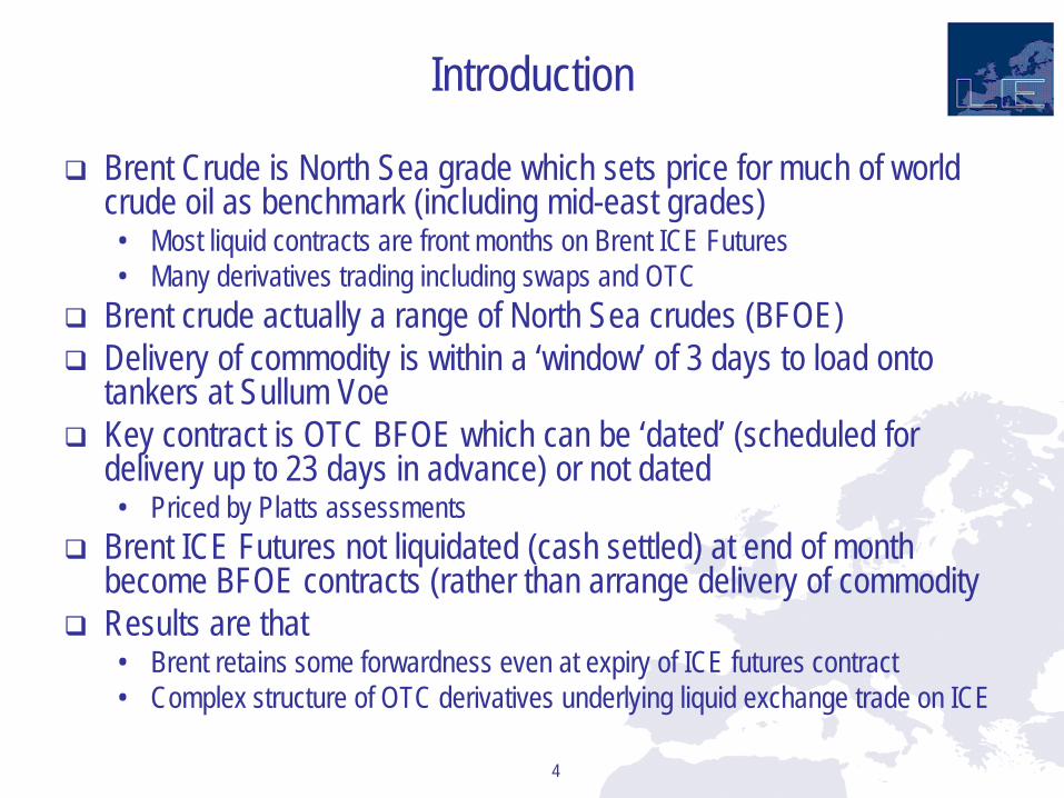
Introduction

Brent Crude is North Sea grade which sets price for much of world crude oil as benchmark (including mid-east grades) • Most liquid contracts are front months on Brent ICE Futures • Many derivatives trading including swaps and OTC

Brent crude actually a range of North Sea crudes (BFOE) Delivery of commodity is within a ‘window’ of 3 days to load onto

tankers at Sullum Voe Key contract is OTC BFOE which can be ‘dated’ (scheduled for

delivery up to 23 days in advance) or not dated • Priced by Platts assessments

Brent ICE Futures not liquidated (cash settled) at end of month become BFOE contracts (rather than arrange delivery of commodity

Results are that • Brent retains some forwardness even at expiry of ICE futures contract • Complex structure of OTC derivatives underlying liquid exchange trade on ICE

4

Previous research

Very little done precisely on how to detect anomalies First review of theory of storage and cash and carry

• The foundations of pricing research for storable commodities is based on the “theory of storage” and the notion of intertemporal cash and carry arbitrage [Kaldor (1939), Working (1948, 1949), Telser (1958) and Williams & Wright (1991)]

Geman and Smith (2012) consider the general theory of storage and propose a model for calendar spreads in precision metals futures prices.

The calendar spread is the difference between two prices for the same commodity but with different delivery dates.

• They show that the interest and storage cost adjusted spread is equal to the convenience yield.

• Key insight is that in normal contango situations, cost of carry relationships should govern the relationships between spot and forward prices, but in times of scarcity, when backwardation is likely, then convenience yield would dominate the cost of carry in the relationship. − Contango is the state of the forward market where the price rises as the time-to-delivery

increases. Backwardation is the opposite.

5

Previous research

Original work by Working in 30s showed relationships between calendar spreads and stocks—indicates convenience yields

6

Previous research

7

Methods Formula for Differential in Calendar Spreads

8

Methods

9

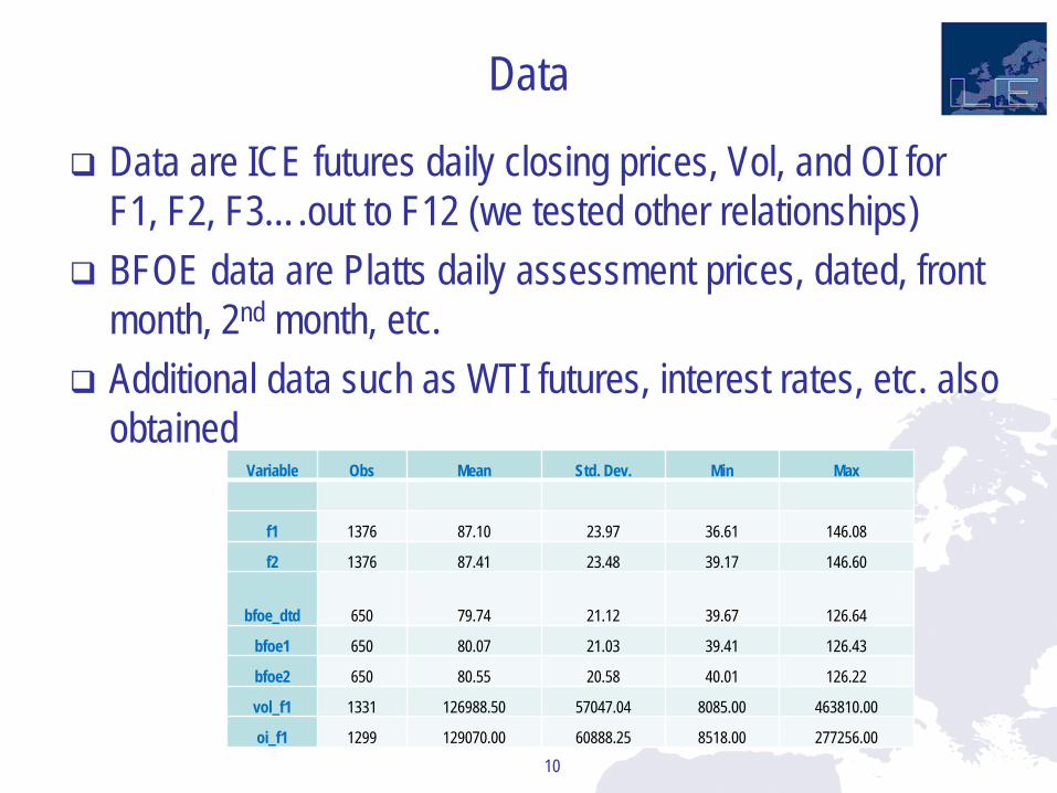
Data

Data are ICE futures daily closing prices, Vol, and OI for F1, F2, F3….out to F12 (we tested other relationships)

BFOE data are Platts daily assessment prices, dated, front month, 2nd month, etc.

Additional data such as WTI futures, interest rates, etc. also obtained

10

Variable Obs Mean Std. Dev. Min Max

f1 1376 87.10 23.97 36.61 146.08

f2 1376 87.41 23.48 39.17 146.60

bfoe_dtd 650 79.74 21.12 39.67 126.64

bfoe1 650 80.07 21.03 39.41 126.43

bfoe2 650 80.55 20.58 40.01 126.22

vol_f1 1331 126988.50 57047.04 8085.00 463810.00

oi_f1 1299 129070.00 60888.25 8518.00 277256.00

Results

The a priori test to identify periods of potential manipulation of Berrera-Rey and Seymour • Eight periods identified

11

Period bfoe_dtd bfoe1 bfoe2

12/07/09 - 15/07/09 59.44 60.45 60.27

27/07/09 - 31/07/09 67.89 68.59 68.50

09/09/10- 14/09/09 78.00 78.57 78.51

15/12/10 - 25/12/10 92.46 93.06 92.97

10/01/11 - 21/01/11 97.77 98.60 98.01

28/02/11 - 05/03/11 114.90 115.58 115.42

16/06/11 - 02/07/11 109.84 110.48 110.16

19/07/11 - 30/07/11 118.16 119.15 118.22

Results

12

(1) (2) (3) (4) (5) (6) (7) (8) (9) VARIABLES D0 D1 D2 D3 D4 D5 D6 D7 D_all lnsprd_bfoe1_dtd 0.216533*** 0.219551*** 0.215330*** 0.215349*** 0.220204*** 0.215285*** 0.214900*** 0.214434*** 0.232484*** (0.038) (0.039) (0.039) (0.039) (0.039) (0.039) (0.039) (0.039) (0.039) td -0.000031*** -0.000031*** -0.000031*** -0.000031*** -0.000030*** -0.000031*** -0.000031*** -0.000031*** -0.000030*** (0.000) (0.000) (0.000) (0.000) (0.000) (0.000) (0.000) (0.000) (0.000) d0 0.218147 (0.542) d0_lnsprd_bfoe1_dtd -0.540388 (1.288) d1 0.195150 (0.579) d1_lnsprd_bfoe1_dtd -0.477411 (1.391) d2 -3.296022 (7.646) d2_lnsprd_bfoe1_dtd 7.983354 (18.527) d3 0.097088 (0.393) d3_lnsprd_bfoe1_dtd -0.240237 (0.954) d4 0.406854 (0.339) d4_lnsprd_bfoe1_dtd -0.991563 (0.821) d5 0.466335 (1.083) d5_lnsprd_bfoe1_dtd -1.135225 (2.630) d6 0.118667 (0.356) d6_lnsprd_bfoe1_dtd -0.287880 (0.865) d7 0.041272 (0.333) d7_lnsprd_bfoe1_dtd -0.098485 (0.809) d_all 0.267508** (0.119) d_all_lnsprd_bfoe1_dtd -0.652445** (0.287) Constant 0.483895*** 0.480950*** 0.483215*** 0.482919*** 0.479988*** 0.483278*** 0.483630*** 0.483949*** 0.472468*** (0.035) (0.035) (0.035) (0.035) (0.035) (0.035) (0.035) (0.035) (0.035) Observations 903 903 903 903 903 903 903 903 903 R-squared 0.398443 0.400592 0.398535 0.399305 0.401014 0.398761 0.398811 0.398698 0.403156

Results

13

(1) (2) (3) (4) (5) (6) (7) (8) (9) (10) VARIABLES D0 D1 D2 D3 D4 D5 D6 D7 D_a_vol D_a_wti lnsprd_bfoe1_dtd 0.135702*** 0.131767*** 0.131680*** 0.137272*** 0.128496*** 0.125412*** 0.130413*** 0.130103*** 0.145660*** 0.155433*** (0.034) (0.034) (0.034) (0.034) (0.034) (0.034) (0.034) (0.034) (0.035) (0.032) td -0.000034*** -0.000034*** -0.000034*** -0.000034*** -0.000034*** -0.000034*** -0.000034*** -0.000034*** -0.000034*** -0.000018*** (0.000) (0.000) (0.000) (0.000) (0.000) (0.000) (0.000) (0.000) (0.000) (0.000) d1 0.165689 (0.454) d1_lnsprd_bfoe1_dtd -0.404459 (1.091) lnvol_f1 0.000636** 0.000631** 0.000616** 0.000660** 0.000632** 0.000635** 0.000635** 0.000640** 0.000614** 0.000685** (0.000) (0.000) (0.000) (0.000) (0.000) (0.000) (0.000) (0.000) (0.000) (0.000) lnoi_f1 -0.000155 -0.000141 -0.000136 -0.000190 -0.000154 -0.000153 -0.000154 -0.000159 -0.000117 -0.000083 (0.000) (0.000) (0.000) (0.000) (0.000) (0.000) (0.000) (0.000) (0.000) (0.000) winter 0.006021*** 0.006015*** 0.006059*** 0.006066*** 0.006540*** 0.006483*** 0.006061*** 0.006057*** 0.005925*** 0.003743*** (0.001) (0.001) (0.001) (0.001) (0.001) (0.001) (0.001) (0.001) (0.001) (0.001) d2 -2.951843 (6.120) d2_lnsprd_bfoe1_dtd 7.150828 (14.830) d3 0.060288 (0.310) d3_lnsprd_bfoe1_dtd -0.149719 (0.754) d4 0.401245 (0.267) d4_lnsprd_bfoe1_dtd -0.977254 -0.006632 (0.647) (0.006) d5 0.005645 0.384008 (0.003) (0.859) d5_lnsprd_bfoe1_dtd -0.919015 (2.085) d6 0.032194 (0.284) d6_lnsprd_bfoe1_dtd -0.074446 (0.691) d7 -0.034872 (0.272) d7_lnsprd_bfoe1_dtd 0.089247 (0.662) d_all 0.254750*** 0.263956*** (0.095) (0.093) d_all_lnsprd_bfoe1_dtd -0.618749*** -0.641424*** (0.230) (0.225) lnsprd_wtif2_1 0.452066*** (0.039) lnsprdf3bfoe2 0.040206*** (0.008) Constant 0.576649*** 0.578848*** 0.578589*** 0.575197*** 0.581192*** 0.583650*** 0.580836*** 0.580911*** 0.570747*** 0.259272*** (0.035) (0.035) (0.035) (0.034) (0.035) (0.035) (0.035) (0.035) (0.035) (0.039) Observations 844 844 844 844 844 844 844 844 844 821 R-squared 0.468698 0.466530 0.467888 0.470570 0.469174 0.465966 0.468292 0.468123 0.467604 0.625657

Results

The test of whether the two coefficients are equal • The difference is significant for all but the first period

14

Dummy 0 lnsprd_bfoe1_dtd - d0_lnsprd_bfoe1_dtd = 0 F( 1, 645) = 0.48 Prob > F = 0.4893








Conclusions

Fundamentally we are testing • If contango and backwardation exists simultaneously in front month contracts

− Hypothesis that these two cannot coexist in short time period and be explained by storage or cash and carry

• If relationship between calendar spreads changes significantly for identified periods

Results confirm that a number of periods identified cannot reject above hypothesis

Usefulness in that more formally shows how previous test fits with theory of storage/cash and carry and performs formal statistical test

Still conclusions need to be weak because cannot ‘prove’ a starting hypothesis, thus we merely say that we’ve identified anomalies or a priori evidence of price manipulation

Useful still as investigations would then proceed to focus on gathering more evidence around the time periods identified

15

Conclusions

Conclusion

16

Documents

Detecting abnormalities in the Brent crude oil commodities and derivatives pricing complexlondoneconomics.co.uk/wp-content/uploads/2013/11/Br… · · 2013-11-25Detecting abnormalities