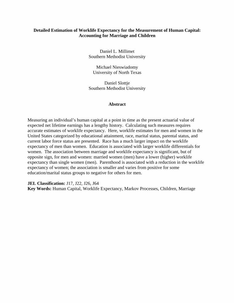
Detailed Estimation of Worklife Expectancy for the Measurement of Human Capital: Accounting for Marriage and Children

Daniel L. Millimet Southern Methodist University

Michael Nieswiadomy

University of North Texas

Daniel Slottje Southern Methodist University

Abstract Measuring an individual’s human capital at a point in time as the present actuarial value of expected net lifetime earnings has a lengthy history. Calculating such measures requires accurate estimates of worklife expectancy. Here, worklife estimates for men and women in the United States categorized by educational attainment, race, marital status, parental status, and current labor force status are presented. Race has a much larger impact on the worklife expectancy of men than women. Education is associated with larger worklife differentials for women. The association between marriage and worklife expectancy is significant, but of opposite sign, for men and women: married women (men) have a lower (higher) worklife expectancy than single women (men). Parenthood is associated with a reduction in the worklife expectancy of women; the association is smaller and varies from positive for some education/marital status groups to negative for others for men. JEL Classification: J17, J22, J26, J64 Key Words: Human Capital, Worklife Expectancy, Markov Processes, Children, Marriage

1

1. Introduction

Dating back at least until the work of Farr (1853), one measure of an individual’s

human capital is the present actuarial value of his or her expected net lifetime earnings.

Dublin and Lotka (1930) extended the work of Farr (1853) by allowing for the possibility

of non-employment, and Jorgenson and Fraumeni (1989, 1992) incorporate an

individual’s gender, age, and education into the analysis. Le et al. (2003, 2006) and

Oxley et al. (2008) provide an extensive review and apply the Jorgenson and Fraumeni

approach to the measurement of human capital in New Zealand. See Folloni and

Vittadini (2010) for an excellent survey, as well as Wöβmann (2003) for a discussion of

human capital measurement in the context of the empirical growth literature. Finally, see

Tchernis (2010) for a detailed analysis of the role of prior employment spells on human

capital accumulation and lifetime wage paths.

Under this approach to human capital measurement, accurate data on worklife

expectancies are required.1 In the United States, the U.S. Bureau of Labor Statistics

(BLS) first published worklife tables in 1950. However, the most recent BLS revision

occurred in 1986 (BLS, 1986) and thus do not reflect recent changes in labor force

participation rates. For instance, labor force participation rates (LFPR) for men (aged 16

and above) declined from 77.4% in 1980 to 74.9% in 1998, while the rate increased for

women from 51.5% in 1980 to 59.8% in 1998 (Fullerton, 1999). In the past decade, the

male LFPR has continued to decline to 72.3% in December 2008, while the female LFPR

has remained around 59% (59.5% in December 2008) (BLS, 2009).

Millimet et al. (2003) recently updated the BLS worklife tables and provided a

new econometric method for estimating worklife expectancies. The authors estimate

worklife expectancies by gender, age, education, and race. In this paper, we utilize the

Millimet et al. (2003) methodology to construct even more detailed worklife tables based

on gender, age, education, race, marital status and parental status, conditional on current

labor force status. These detailed estimates enable one to obtain much more precise

measures of the stock of human capital.

Accounting for individual attributes such as marital status and parental status in

worklife expectancies is likely to be very important. First, as articulated in Wöβmann

1 Worklife expectancies are also extensively utilized to project lost earnings (see, e.g., Nieswiadomy and Slottje, 1988; Nieswiadomy and Silberberg, 1988; Skoog and Ciecka, 2001, 2002).

2

(2003), Lovaglio (2010), and elsewhere, human capital is a complex concept,

incorporating and depending on many underlying factors. Family background is one

such factor. As such, observable attributes reflecting family background should play a

salient role in any measure of human capital.

Second, beginning with the seminal work of Mincer and Polachek (1974), the

impact of children and marriage on labor supply, housework, and earnings has received

considerable attention in the human resources literature (e.g., Klerman and Leibowitz,

1999; Waldfogel, 1998; and Polachek and Siebert 1996). For example, Lundberg (1988)

finds that labor supply of husbands and wives is jointly determined only when young

children are present. Hersch and Stratton (1994) analyze the division of housework for

employed spouses, finding significant interactions between the time allocation of

husbands and wives, their education, and the presence of children under age 12. Angrist

and Evans (1998), Millimet (2000), Ebenstein (2008) and others document a significant,

negative effect of children on the labor supply of married women, but no corresponding

effect on the time allocation of men. Millimet (2000) also finds a positive impact of

children on the wages of men, while Waldfogel (1998), Hersch and Stratton (1997) and

others discuss the “motherhood wage penalty.” Finally, a number of studies provide

empirical evidence in support of the marriage premium: the fact that married men earn

more on average than single men even after controlling for common measures of human

capital (e.g., Chun and Lee, 2001; Loh, 1996; Maasoumi et al. 2009).

Despite this rich literature examining the interplay between family life and labor

market interactions, no study (to our knowledge) has analyzed the association between

these attributes and worklife expectancy.2 In addition, our worklife estimates differ from

the earlier BLS approach in three other respects. First, we use the 1992 through 2001

March Annual Demographic Surveys in the Current Population Survey (CPS) reports.

We use multiple years to account for a wide variety of economic impacts on labor supply,

as well as to ensure that our results are not influenced by any particular business cycle.

Second, we use an econometric model, rather than a simple relative frequency model.

This econometric approach enables us to compile detailed worklife tables by race,

education, marital status, and parental status, in addition to age and gender. Third, our

2 In related work, Booth et al. (1999) examine work propensities over a several year period using the British Household Panel Survey for men and women and decompose these propensities into observable and unobservable components.

3

approach uses three labor force states: employed, unemployed and inactive (out of the

labor force), in contrast to the BLS method that categorized persons as active (in the labor

force) or inactive (out of the labor force). In the BLS two-state model, an individual's

worklife at a particular age represents the number of years the individual is expected to

remain in the labor force, not necessarily the number of years spent working. Our model

differs because it defines worklife as the expected number of employed years remaining

in a person's life.

The remainder of the paper is organized as follows. The next section discusses

the decisions households must make and their possible impact on worklife expectancy.

Section three presents the methodology. Section four discusses the data. Section five

presents our econometrically estimated worklife tables. Section six concludes.

2. Household Decisions

Every household faces the decision of how to efficiently allocate its time between

labor market and non-market pursuits. In the standard neo-classical model of time

allocation, when there is only one adult (and no children) in the household, that decision

depends on the market wage, non-labor income, and individual preferences for

consumption versus leisure. For single-adult households with children, the decision

becomes more complex. Now, the allocation of time between the labor market and the

home will also depend on preferences for time spent with children, the relative quality of

market-based versus own-provided child care, the cost of market-provided child care, and

any social insurance benefits to which the household is entitled (e.g., Aid to Families

with Dependent Children (AFDC), replaced by Temporary Aid to Needy Families

(TANF) in 1996).3 The host of factors involved in the time allocation decisions of single

parents – relative to single individuals without children – makes the effect of children on

worklife expectancy ambiguous.

In households with two adults, determining the time allocation of each individual

becomes more challenging, even without children present. In the standard economic

framework, the household must decide on the utility-maximizing combination of home-

produced and market-produced goods, subject to the household's budget constraint and

production functions of the husband and wife for home-produced goods. Once this

optimal bundle is known, the household must allocate the time of each spouse to market

3 See Blundell and MaCurdy (1999) for an in-depth analysis of labor supply models.

4

and non-market work. Even assuming identical productivity for men and women in the

production of home-produced goods (e.g., a clean house or a home cooked dinner),

women often have a comparative advantage in these endeavors because of their lower

market wage.4 According to this logic, one might expect married men to work more than

their single counterparts, but for marriage to have the opposite effect on women.

However, the effect on worklife expectancy is distinct from the predictions of this static

framework since marriage may also influence retirement decisions in a more complex,

dynamic model. Thus, the overall effect of marriage on worklife expectancy is

ambiguous. Finally, it is fairly straightforward to extend the static analysis of a two-adult

household to one with children by assuming that one of the home-produced goods being

“produced” represents children. Consequently, the presence of children adds more

variables into the decision-making process of married couples, but does not alter the fact

that marriage has an ambiguous effect on worklife expectancy. Furthermore, comparing

married individuals, by gender, with and without children is also ambiguous (both for

static time allocation, as well as worklife expectancy) since the relative quality and cost

of home-produced child care now become relevant considerations.

Prior to continuing, a final comment is warranted. Our discussion heretofore of

both children and marriage has presumed both decisions to be exogenous. Since this is

not likely to be the case, the association between children, marriage, and worklife

expectancy also reflects any unobserved attributes correlated with these decisions as well

as decisions concerning labor supply. In our empirical analysis, our differences in

worklife estimates across individuals differentiated on the basis of children or marital

status reflect these associations and, hence, should not be interpreted as causal effects.

That said, since our motivation stems from improved measurement of human capital, and

4 The likelihood that married men have a comparative advantage in market labor are increased by the marriage premium. Chun and Lee (2001) investigate one possible reason for the marriage premium: married men earn more because they are able to specialize in labor market activities, whereas their wives specialize in home production. Chun and Lee (2001) verify that the marriage premium decreases the more one's wife works. Loh (1996) and Maasoumi et al. (2009) examine the household specialization hypothesis, as well as two other theories behind the marriage premium: (i) positive selection (i.e., unobservables associated with higher earnings are valued in the marriage market), and (ii) employer discrimination (i.e., employers favor married men, viewing them as more responsible or less mobile). While these, and other such, analyses provides insight into the origin of the earnings differential of married and single men, it does not help determine the differences in worklife expectancy across married and single men since the standard income and substitution effects are ambiguous. On the one hand, married men may work more years than single men due to their higher wage (the substitution effect). On the other hand, married men may choose to “buy” more time with their family (the income effect).

5

not estimation of the effect of exogenous changes in children or marital status, this

“weaker” interpretation of our findings is not problematic.

3. The Econometrically Estimated Worklife Model

The BLS (1986) worklife tables categorize individuals into two types: active and

inactive. The active category includes all individuals in the labor force (employed and

unemployed). The BLS's inclusion of the unemployed among the active is based on the

assumption that the unemployed are more similar to the employed than those out of the

labor force. The BLS (1982, p. 2) states, “It has long been recognized that persons who

are already in the labor force are more likely to work in the future than are those not

currently active.” However, the result of this pooling is that the BLS definition of

“worklife” is not comparable to the number of remaining working years due to the

inclusion of the unemployed in the active category. Thus, the BLS (1986) “worklife”

expectancies overestimate the actual worklife (i.e., the remaining years of employment)

of the currently active, and may exaggerate the worklife of the unemployed if their labor

force behavior is more like that of the inactive. For example, Hall (1970), Clark and

Summers (1979, 1982), Tano (1991), Flinn and Heckman (1983), Gönül (1992), and

Jones and Riddell (1999) find that the distinction between the unemployed and inactive is

fuzzy. Many individuals bounce between periods of unemployment and labor force

inactivity within a given nonemployment spell. However, rather than simply re-defining

the inactive group to include the unemployed, we allow for three distinct groups by

estimating a multinomial logit for the three labor market states (employed, unemployed

and inactive).5 We estimate the model on three distinct subsets of the data: individuals

initially employed, initially unemployed, and initially inactive. We then use the estimates

to estimate the nine relevant age-specific transition probabilities described below.

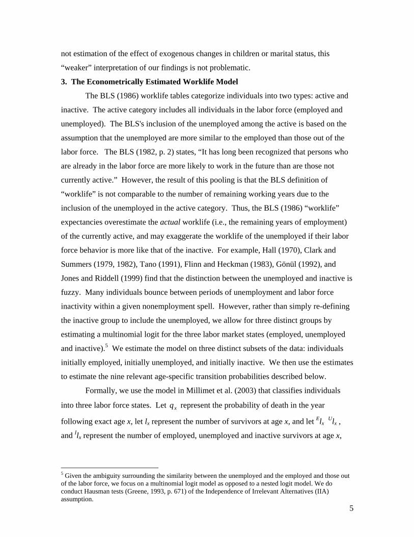
Formally, we use the model in Millimet et al. (2003) that classifies individuals

into three labor force states. Let xq represent the probability of death in the year

following exact age x, let lx represent the number of survivors at age x, and let Elx Ulx ,

and Ilx represent the number of employed, unemployed and inactive survivors at age x,

5 Given the ambiguity surrounding the similarity between the unemployed and the employed and those out of the labor force, we focus on a multinomial logit model as opposed to a nested logit model. We do conduct Hausman tests (Greene, 1993, p. 671) of the Independence of Irrelevant Alternatives (IIA) assumption.

6

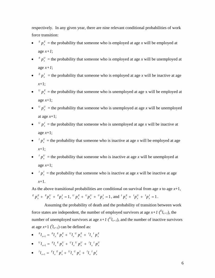
respectively. In any given year, there are nine relevant conditional probabilities of work

force transition:

• Ex

E p = the probability that someone who is employed at age x will be employed at

age x+1;

• Ux

E p = the probability that someone who is employed at age x will be unemployed at

age x+1;

• Ix

E p = the probability that someone who is employed at age x will be inactive at age

x+1;

• Ex

U p = the probability that someone who is unemployed at age x will be employed at

age x+1;

• Ux

U p = the probability that someone who is unemployed at age x will be unemployed

at age x+1;

• Ix

U p = the probability that someone who is unemployed at age x will be inactive at

age x+1;

• Ex

I p = the probability that someone who is inactive at age x will be employed at age

x+1;

• Ux

I p = the probability that someone who is inactive at age x will be unemployed at

age x+1;

• Ix

I p = the probability that someone who is inactive at age x will be inactive at age

x+1.

As the above transitional probabilities are conditional on survival from age x to age x+1,

1=++ Ix

EUx

EEx

E ppp , 1=++ Ix

UUx

UEx

U ppp , and 1=++ Ix

IUx

IEx

I ppp .

Assuming the probability of death and the probability of transition between work

force states are independent, the number of employed survivors at age x+1 (Elx+1), the

number of unemployed survivors at age x+1 (Ulx+1), and the number of inactive survivors

at age x+1 (Ilx+1) can be defined as:

• Ex

Ix

IEx

Ux

UEx

Ex

Ex

E plplpll ++=+1

• Ux

Ix

IUx

Ux

UUx

Ex

Ex

U plplpll ++=+1

• Ix

Ix

IIx

Ux

UIx

Ex

Ex

I plplpll ++=+1

7

where lx = Elx + Ulx+ Ilx and lx+1 = lx(1 – qx).

It is assumed that persons who die, become employed, become unemployed, or become

inactive in a given year do so at mid-year. According to this Markov process with one-

period memory, the transition probabilities do not depend on previous transition

probabilities.

The BLS calculated its 1986 increment-decrement tables by using relative

frequency process to matched CPS data from the 1979 - 1980 survey. The BLS's

worklife tables are sub-divided based on education or race, but not both at the same time,

due to insufficient sample size. For similar reasons, marital status and parental status

could not be used in constructing worklife tables. Yet, as stated previously, it is well

known that labor supply decisions depend on these factors (see also Killingsworth, 1983).

To account for these factors we estimate the transition probabilities as a function of

marital status, number of children present in the home, age, race, gender, and education.

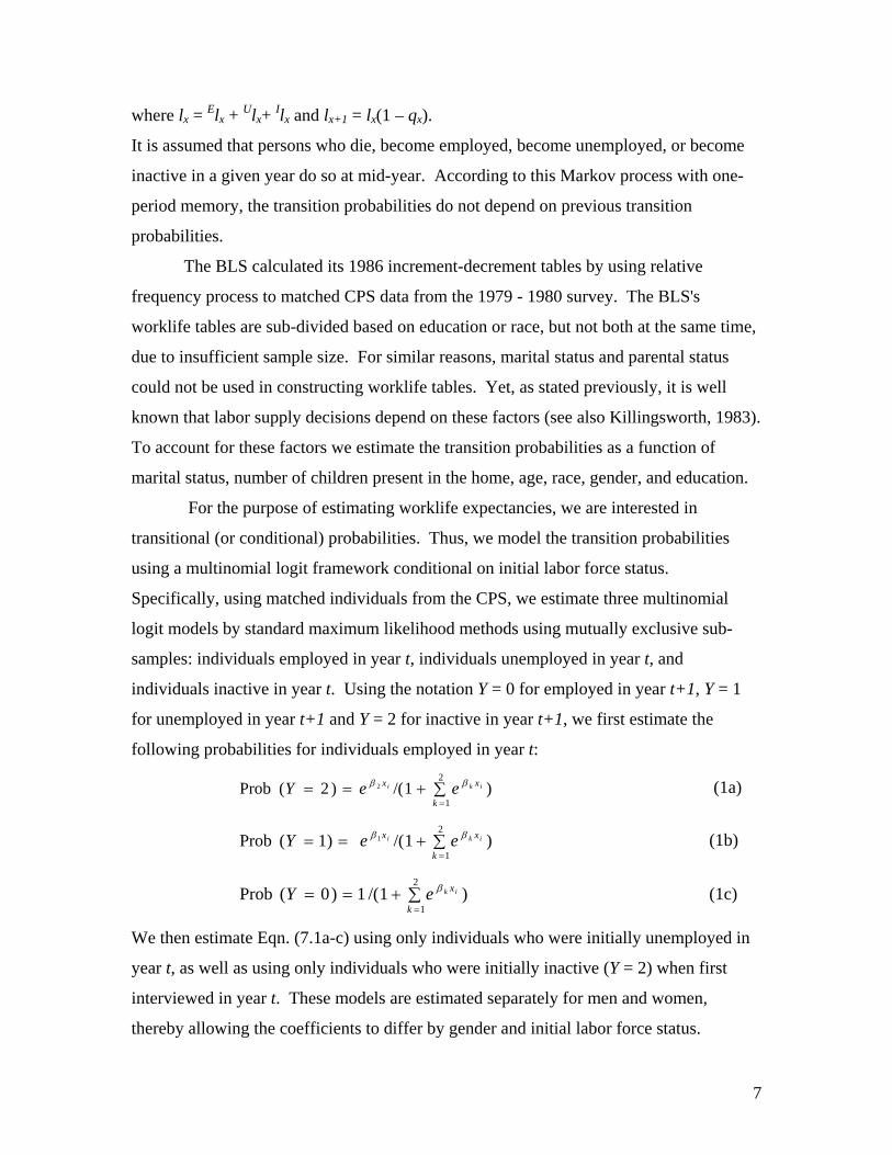
For the purpose of estimating worklife expectancies, we are interested in

transitional (or conditional) probabilities. Thus, we model the transition probabilities

using a multinomial logit framework conditional on initial labor force status.

Specifically, using matched individuals from the CPS, we estimate three multinomial

logit models by standard maximum likelihood methods using mutually exclusive sub-

samples: individuals employed in year t, individuals unemployed in year t, and

individuals inactive in year t. Using the notation Y = 0 for employed in year t+1, Y = 1

for unemployed in year t+1 and Y = 2 for inactive in year t+1, we first estimate the

following probabilities for individuals employed in year t:

)1/()2(Prob2

1

2 ∑+===k

xx iki eeY ββ (1a)

)1/()1(Prob2

1

1 ∑+===k

xx iki eeY ββ (1b)

)1/(1)0(Prob2

1∑+===k

xikeY β (1c)

We then estimate Eqn. (7.1a-c) using only individuals who were initially unemployed in

year t, as well as using only individuals who were initially inactive (Y = 2) when first

interviewed in year t. These models are estimated separately for men and women,

thereby allowing the coefficients to differ by gender and initial labor force status.

8

The x vector in Eqn. (7.1a-c) includes controls for: age, age squared, a race

dummy, race interacted with age and age squared, marriage dummy, marriage dummy

times age, number of children under six, number of children under 18, each child variable

interacted with age, occupation dummies, occupation dummies interacted with age, and

time dummies. We use four occupation categories: managerial and professional;

technical, sales and administrative; service; and operators and laborers.6

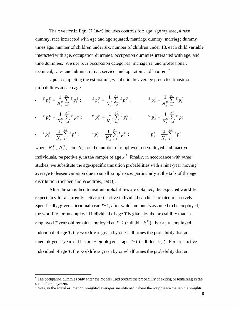
Upon completing the estimation, we obtain the average predicted transition

probabilities at each age:

• ∑=

=ExN

i

Ei

EEx

Ex

E pN

p1

1 ; ∑=

=ExN

i

Ui

EEx

Ux

E pN

p1

1 ; ∑=

=ExN

i

Ii

EEx

Ix

E pN

p1

1

• ∑=

=UxN

i

Ei

UUx

Ex

U pN

p1

1 ; ∑=

=UxN

i

Ui

UUx

Ux

U pN

p1

1 ; ∑=

=UxN

i

Ii

UUx

Ix

U pN

p1

1

• ∑=

=IxN

i

Ei

IIx

Ex

I pN

p1

1 ; ∑=

=IxN

i

Ui

IIx

Ux

I pN

p1

1 ; ∑=

=IxN

i

Ii

IIx

Ix

I pN

p1

1

where ExN , U

xN , and IxN are the number of employed, unemployed and inactive

individuals, respectively, in the sample of age x.7 Finally, in accordance with other

studies, we substitute the age-specific transition probabilities with a nine-year moving

average to lessen variation due to small sample size, particularly at the tails of the age

distribution (Schoen and Woodrow, 1980).

After the smoothed transition probabilities are obtained, the expected worklife

expectancy for a currently active or inactive individual can be estimated recursively.

Specifically, given a terminal year T+1, after which no one is assumed to be employed,

the worklife for an employed individual of age T is given by the probability that an

employed T year-old remains employed at T+1 (call this ET

E ). For an unemployed

individual of age T, the worklife is given by one-half times the probability that an

unemployed T year-old becomes employed at age T+1 (call this UT

E ). For an inactive

individual of age T, the worklife is given by one-half times the probability that an

6 The occupation dummies only enter the models used predict the probability of exiting or remaining in the state of employment. 7 Note, in the actual estimation, weighted averages are obtained, where the weights are the sample weights.

9

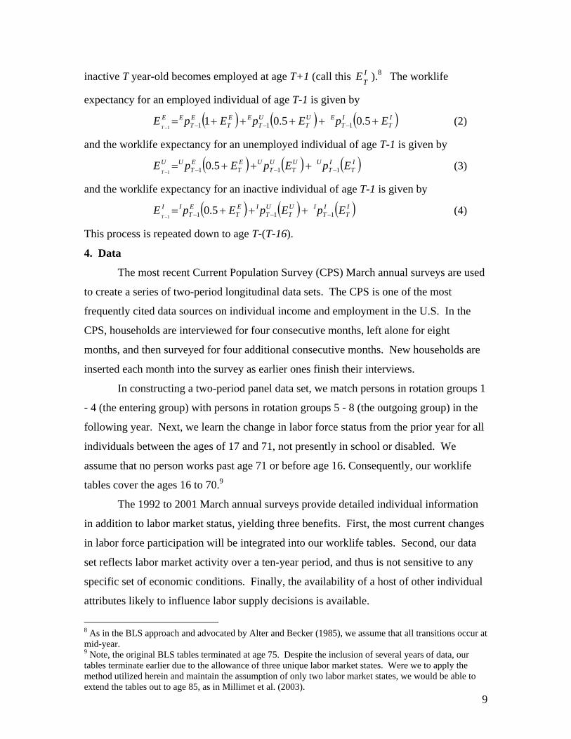
inactive T year-old becomes employed at age T+1 (call this ITE ).8 The worklife

expectancy for an employed individual of age T-1 is given by

( ) ( ) ( )IT

IT

EUT

UT

EET

ET

EE EpEpEpET

+++++= −−−−5.05.01 1111

(2)

and the worklife expectancy for an unemployed individual of age T-1 is given by

( ) ( ) ( )IT

IT

UUT

UT

UET

ET

UU EpEpEpET 111 5.0

1 −−− +++=−

(3)

and the worklife expectancy for an inactive individual of age T-1 is given by

( ) ( ) ( )IT

IT

IUT

UT

IET

ET

II EpEpEpET 111 5.0

1 −−− +++=−

(4)

This process is repeated down to age T-(T-16).

4. Data

The most recent Current Population Survey (CPS) March annual surveys are used

to create a series of two-period longitudinal data sets. The CPS is one of the most

frequently cited data sources on individual income and employment in the U.S. In the

CPS, households are interviewed for four consecutive months, left alone for eight

months, and then surveyed for four additional consecutive months. New households are

inserted each month into the survey as earlier ones finish their interviews.

In constructing a two-period panel data set, we match persons in rotation groups 1

- 4 (the entering group) with persons in rotation groups 5 - 8 (the outgoing group) in the

following year. Next, we learn the change in labor force status from the prior year for all

individuals between the ages of 17 and 71, not presently in school or disabled. We

assume that no person works past age 71 or before age 16. Consequently, our worklife

tables cover the ages 16 to 70.9

The 1992 to 2001 March annual surveys provide detailed individual information

in addition to labor market status, yielding three benefits. First, the most current changes

in labor force participation will be integrated into our worklife tables. Second, our data

set reflects labor market activity over a ten-year period, and thus is not sensitive to any

specific set of economic conditions. Finally, the availability of a host of other individual

attributes likely to influence labor supply decisions is available.

8 As in the BLS approach and advocated by Alter and Becker (1985), we assume that all transitions occur at mid-year. 9 Note, the original BLS tables terminated at age 75. Despite the inclusion of several years of data, our tables terminate earlier due to the allowance of three unique labor market states. Were we to apply the method utilized herein and maintain the assumption of only two labor market states, we would be able to extend the tables out to age 85, as in Millimet et al. (2003).

10

Our matching algorithm is similar to Peracchi and Welch (1995). First, we match

households in rotations 1 - 4 in one year with the same household (using the unique

household identification number) the following year in rotations 5 - 8. Second, we

require that an individual in a matched household must have the same sex and race, and

must be one year older, when interviewed in rotations 5 - 8. We should note the CPS

does not follow movers, which may lead to a nonrandom attrition problem. Fortunately,

Peracchi and Welch (1995) discovered no systematic bias in transition estimates after

controlling for sex, age, and labor force status at the time of the first survey, based on 13

years (1979 - 1991) of CPS data. Peracchi and Welch (1995) matched two-thirds of their

March annual surveys from 1979 to 1991. Similarly, we are able to match

approximately 63% of our 1992 - 2001 samples. (1993 cannot be matched with 1994,

and 1995 cannot be matched with 1996 because of survey modifications.)

To allow comparison to previous worklife tables, we sort the data by sex and

education, as represented in the BLS 1986 study. Our three educational categories are

nearly identical to those of the BLS: less than a high school degree, high school degree to

some college, and a college degree and above.10 In addition, we utilize data on marital

status, race, number of children under age six, number of children under age 18, and

occupation. Finally, we include the appropriate sampling weights not only when

estimating the multinomial logit models, but also when obtaining the mean age-specific

transition probabilities.

5. Empirical Results

Tables 1 through 6 present the worklife expectancies obtained after permitting

three unique labor force states (employed, unemployed and inactive).11 We do not

present the full tables, but they are available at

http://faculty.smu.edu/millimet/pdf/worklifekids.pdf. In order to construct the worklife

tables for women with children, we assume that a woman has the typical number of

children based on the demographic statistics from the Census Bureau. Specifically, we

assume that a married woman with less than a high school degree has three children at

ages 22, 25, and 28. A married woman with a high school degree has two children at

10 The BLS's second and third categories were somewhat different. The BLS second category was high school degree to 14 years of schooling and the third category was 15 or more years of schooling. 11 According to the Hausman tests, we cannot reject the Independence of Irrelevant Alternative (IIA) assumption in the majority of the multinomial logit models estimated.

11

ages 22 and 25. A married woman with a college degree has two children at ages 22 and

25. We assume that a single woman with less than a high school degree has two children

at ages 22 and 25. A single woman with a high school degree has one child at age 22. A

single woman with a college degree has one child at age 22. These assumptions of the

number of children and the age of the mother at the time of each birth are only meant to

be approximate.12 We now present the results, first for women, then for men. For both

women and men, we first discuss the relationship between race and worklife expectancy,

then education, marital status, and children.

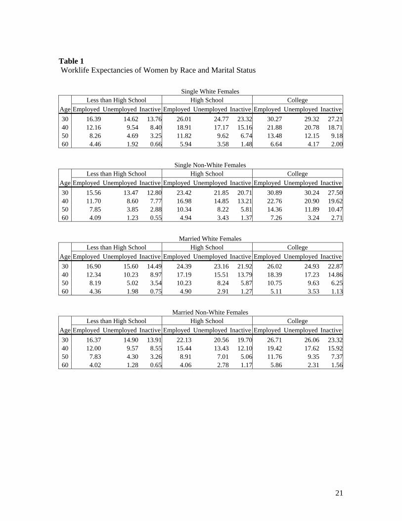
5.1. Women: race, education, and marriage

For women, race has little association with worklife expectancy except for high

school educated women. As shown in Table 1, for employed 30 year-olds, there is less

than a one-year difference between single white and non-white employed women with

college and less than high school education levels; the same is true for married white and

non-white women.13 However, the worklife expectancy of an employed 30 year-old

white woman with a high school degree exceeds that of similar non-white woman by over

two years.

In contrast, the association between educational attainment and worklife

expectancy is more pronounced, especially for single women. As shown in Table 1, a 30

year-old college educated single white female has a worklife expectancy that is 13.9

years longer than a woman with less than a high school degree. A 30 year-old college

educated married white woman has a worklife expectancy that exceeds that for a white

woman with less than a high school degree by 9.1 years. For non-white women, the

differences in worklife expectancies between college and less than high school educated

12 According to a recently released report by the US Centers for Disease Control and Prevention (National Vital Statistics Report, Volume 51, Number 1, 11 December 2002, available at http://www.cdc.gov/nchs/data/nvsr/nvsr51/nvsr51_01.pdf), the average age of first birth in 1970 was 21.4 years of age. In 2000, this has increased to 24.9 years of age. The report does not differentiate age at first birth by education or marital status. As a result, the worklife expectancies presented in this study are more accurate for women in older cohorts. 13 Throughout the discussion of the results, it is important to bear two caveats in mind. First, worklife estimates are estimated conditional on current labor force status (e.g., employed, unemployed, or inactive); the relationship between race or any other demographic characteristics of individuals and current labor force status is ignored. Thus, while race appears unrelated to, say, the worklife expectancy of single, employed females, race may play a pivotal role in the probability that a single female is employed. Second, in principle there are more than three labor force states into which individuals may be categorized. For example, an unemployed individual with a long history of employment may be fundamentally distinct from an individual who has spent the majority of his or her life unemployed or inactive. Unfortunately, such distinctions are not possible using CPS data.

12

women are slightly larger (15.3 years for singles and 10.3 years for married persons).

Moreover, when comparing college to the high school level, race matters as well. For

instance, the worklife expectancy of a 30 year-old college educated single white woman

is 4.3 years longer than for a white woman with a high school degree; for a non-white

woman the difference is 7.5 years. The worklife expectancy of a 30 year-old college

educated married white woman exceeds the worklife expectancy of her high school

counterpart by 1.6 years; for a non-white woman the difference is 4.6 years.

As expected, the association between marriage and the worklife expectancy of

women is considerable. The relationship is strongest for women with college degrees.

As shown in Table 1, for both white and non-white college educated 30 year-old women,

marriage is associated with a decline in worklife expectancy of roughly 4.2 years. For

white and non-white high school educated women, marriage is associated with about a

1.5 year reduction in worklife expectancy. At the less than high school level, there is

almost no correlation between marital status and worklife expectancy. The negative

association between marriage and worklife expectancy for women with at least a high

school education is consistent with the model of joint labor supply discussed previously.

Specifically, marriage typically results in one spouse specializing in the production of

household goods. Since women tend to (i) be more productive at home, and/or (ii) have a

lower opportunity cost (due to a lower market wage), the labor force participation of

women suffers with marriage.

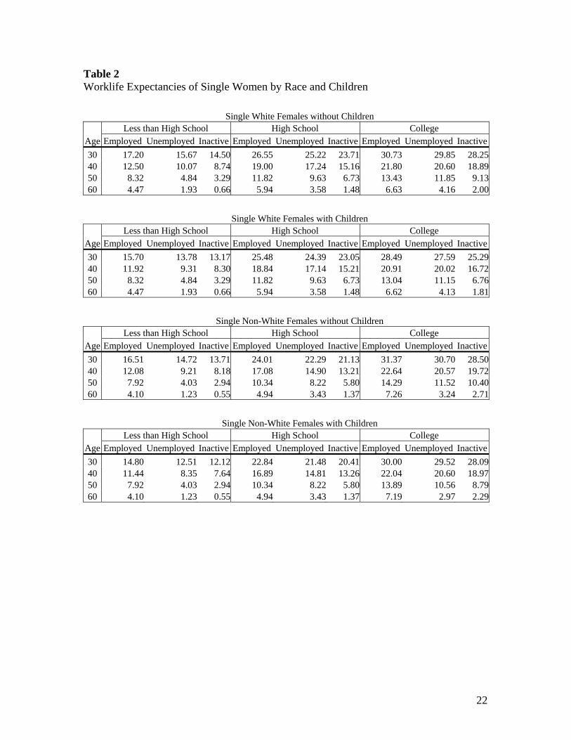
5.2. Women: children

The worklife expectancy of a single woman with children (as described in our

model) is between one and two years lower than a comparable childless woman. As

shown in Table 2, for a 30 year-old employed single white college educated female,

children are associated with a reduction in worklife expectancy of 2.2 years; for a non-

white woman the reduction is 1.4 years. At the high school level the reduction is 1.1 to

1.2 years for single white and non-white women, respectively. Finally, for those with

less than a high school education, worklife expectancy is 1.5 to 1.7 years lower for single

whites and non-whites, respectively.

The worklife expectancy of a married woman with children (as described in our

model) is between one and three years lower than comparable childless woman. As

shown in Table 3, for a 30 year-old employed married white college educated female, the

13

worklife expectancy for women with children is 2.9 years shorter than for similar

childless women; for a non-white woman the reduction is 1.5 years. At the high school

level the reduction associated with children is 1.0 to 1.1 years for married whites and

non-whites, respectively. Lastly, for women without a high school diploma, the

reduction in worklife expectancy is 1.2 to 1.3 years for married whites and non-whites,

respectively.

The negative relationship between children and female worklife expectancy are

consonant with the vast empirical studies documenting the deleterious (causal) effects of

children on female labor force participation (e.g., Millimet, 2000; Angrist and Evans,

1998). Of course, studies of the effects of children on female labor force participation

typically focus on just the impact of young children on labor market behavior (while the

children still reside at home). While differences in the worklife expectancies of women

with and without children reflect these effects, children may also influence worklife

expectancy even when they no longer reside with the parents. For example, adult

children may influence retirement decisions due to income transfers from adult children

to their parents (e.g., Jellal and Wolff, 2000), or due to the desire of the parents to

relocate closer to their adult children to be near grandchildren.

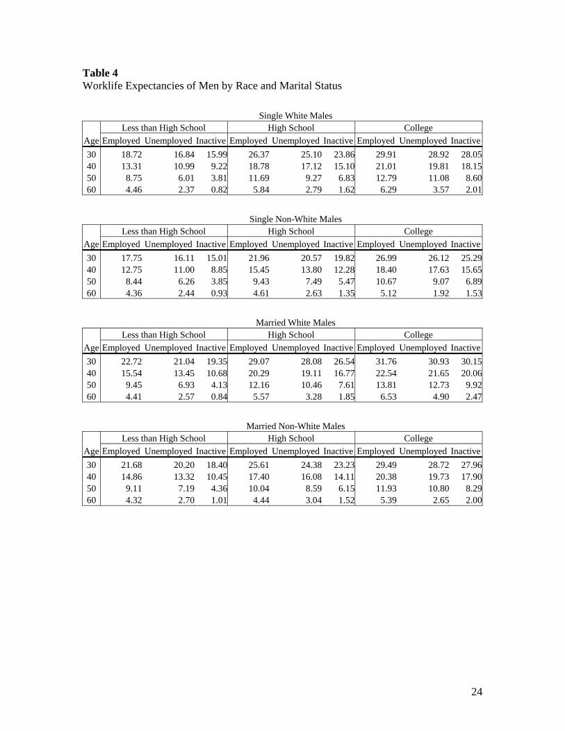
5.3. Men: race, education, and marriage

In contrast to women, the association between race and male worklife expectancy

is particularly acute, with the largest correlation occurring at the high school level. As

shown in Table 4, for employed 30 year-olds with less than a high school education, the

worklife expectancy of single white men exceeds that of similar non-white men by one

year. The same holds for married men. For men with a high school education, the

worklife expectancy of single white men is 4.4 years longer than of similar non-whites;

for married men, the difference is 3.5 years. For men with a college degree, worklife

expectancy is 2.9 years greater for single white men; for married men, the difference is

2.3 years.

Worklife expectancies also vary considerably by educational attainment,

particularly for 30 year-old single white males. However, the association is not as strong

as for women. As shown in Table 4, an employed 30 year-old single white male with a

college education will work, on average, an additional 11.2 years relative to a white male

with a less than high school education. (The comparable differential for women is 13.9

14

years; see Table 1). The difference is of lower magnitude for single non-white males,

with the difference being only 9.2 years (15.3 for comparable women; see Table 1). For

30 year-old married white males, the worklife expectancy of the college educated

exceeds that of similar men with less than high school educated by 9.0 years. For non-

white males, this difference is only 7.8 years.

The differences in worklife expectancy are not as great when comparing college

versus high school educated men. The worklife expectancy of a 30 year-old single white

male with a college education is 3.5 years greater compared with his high school

educated counterpart. The comparable difference for a 30 year-old single non-white male

is 5.0 years. The worklife expectancy of a 30 year-old married white male exceeds that

of a comparable high school educated individual by 2.7 years; for similar non-white

males, the difference is 3.9 years.

Marriage is associated with large differences in worklife expectancy for men of

both races, especially at the high school and less than high school education levels. In

contrast to women, marriage increases worklife expectancies for men. As shown in

Table 4, a 30 year-old married white male with a college-level education works an

additional 1.9 years relative to his single counterpart; an additional 2.5 years for non-

white males. These numbers increase at the high school level. The worklife expectancy

of a 30 year-old married white male exceeds that of a comparable single male by 2.7

years. For a 30 year-old married non-white male, this difference increases to 3.7 years.

Finally, regardless of race, the worklife expectancy of a 30 year-old married male with

less than a high school education exceeds that of a comparable single male by roughly 4.0

years. The positive association between marriage and worklife expectancy is consistent

with marriage premium increasing male labor force participation due to the substitution

effect dominating the income effect.

5.4. Men: children

While the relationship between children and female worklife expectancy is clear,

the association for males varies, mainly across education levels, but also by race.

Moreover, while children are always associated with a reduction in a woman's worklife,

regardless of marital status, this does not hold for men.

For single men with children relative to childless men, worklife expectancy varies

from 1.1 years lower to 2.0 years greater. As shown in Table 5, for a 30 year-old

15

employed single white college educated male, children are associated with a reduction in

worklife expectancy of 1.1 years; for a non-white male, worklife expectancy is 0.2 years

greater. At the high school level, children are associated with a 0.4 to 0.8 year increase in

worklife expectancy for single white and non-white men, respectively. Finally, for males

without a high school education, children are associated with a 2.0 year increase in

worklife expectancy for single white men; a 0.7 year decrease for single non-white men.

The relationship between children and the worklife expectancy of married males

is much weaker than for single males. As shown in Table 6, the worklife expectancy of a

30 year-old employed married college educated male with children is 0.3 to 0.1 years

lower relative to comparable childless men for white and non-white men, respectively.

At the high school level, children are associated with an increase in worklife expectancy

by 0.3 to 0.5 years for married whites and non-whites, respectively. Finally, the worklife

expectancy of married males without a high school diploma with children is 0.4 and 0.3

years lower relative to comparable single males for whites and non-whites, respectively.

For males, married males in particular, the association between children and

worklife expectancy is complex. As documented in Millimet (2000), Angrist and Evans

(1998), and others, the presence of young children in the household has a statistically

insignificant effect on male labor supply. However, children may influence the

retirement behavior of males as discussed above for women. In addition, Millimet (2000)

finds a statistically significant, positive effect of children on the wages of married men,

thus providing an incentive to delay retirement if the substitution effect dominates the

income effect.

6. Conclusion

The correlations between gender, race, education, marital status and children and

labor market behavior have been the focus of much empirical research. In addition,

recent research has investigated the effect of these attributes on the propensity to work

over periods of time (Booth et al. 1999). This paper extends this research by estimating

separate worklife expectancies for individuals differentiated by these attributes. Such

estimates are a vital component of one frequently used measure of human capital: the

present actuarial value of an individual’s expected net lifetime earnings.

To proceed, we utilize the econometric model developed in Millimet et al. (2003)

and current data over a ten-year period (1992 – 2001) from CPS March annual surveys,

16

thus allowing us to construct worklife tables using several demographic characteristics

simultaneously. Relative to previous worklife tables, the estimates presented herein offer

several advantages. First, the econometric approach permits the estimation of much more

detailed worklife expectancy tables compared to the relative frequency approach, which

is limited to using one variable at a time because of sample size problems. Second, our

use of multiple rounds of up-to-date data reduces the sensitivity of the worklife

expectancy estimates to business cycle conditions, as well as reflects the vast changes

that have occurred in the U.S. labor market over the past few decades. Third, our use of a

multinomial logit model to estimate transition probabilities allows us to categorize

individuals into three states: employed, unemployed, and inactive. This avoids the

arbitrary decision of pooling unemployed individuals with either employed individuals or

those out of the labor force, as well as maintains the “true” definition of worklife.

The results indicate that worklife expectancy is sensitive to several factors. First,

even controlling for differences in childbearing and marital status, race has a large

impact, especially for men (up to 4.4 years longer worklife for single white men with

high school degrees). Second, education also matters, particularly for women. The

largest difference occurs between single non-white women with a college education and

similar women with less than a high school degree (where worklife expectancy is 15.3

years greater for the former).

Third, marriage has opposite effects on the worklife expectancies of men and

women. For women, marriage reduces worklife expectancy, where the largest

differential is 4.2 years for married white and non-white women with college degrees

compared to their single counterparts. The largest differential for men is the additional

4.0 years of worklife expectancy for married white males with less than a high school

education relative to comparable single males. Failure to differentiate by marital status,

as in the prior literature, yields estimated worklife expectancies that are weighted

averages of those obtained here (see, e.g., Millimet et al. 2003). Moreover, use of such

weighted averages to construct measures of human capital stock will be less precise and

will not adequately capture changes in marriage trends on the stocks in the future. For

example, the marriage rate declined in every state and Washington D.C. in the United

States between 1990 and 2004 except Hawaii and West Virginia.14

14 See http://www.cdc.gov/nchs/data/nvss/marriage90_04.pdf.

17

Finally, the association between children and worklife expectancy is large and

negative for women; for men, the association varies and is of smaller magnitude. The

largest relationship for women is the 2.9 year reduction in worklife for married white

college educated woman relative to similar childless women. For men, the largest

increase in worklife expectancy (2.0 years) is for single white men with less than a high

school degree, while the largest decrease in worklife expectancy (1.1 years) is for single

white college educated men. Again, failure to incorporate children into estimated

worklife expectancies in the prior literature yields estimates that are weighted averages of

those presented here. Moreover, as stated above, given the heterogeneity in worklife

expectancy by child status, estimates of periodic human capital stocks based on previous

estimates will not adequately reflect changes in fertility rates. For example, in the United

States the total fertility rate rose from 1.84 in 1980 to 2.10 in 2006.15

The multinomial logit method of estimating worklife expectancy offers clear

benefits. A variety of worklife tables, based simultaneously on race, education, sex,

marital status and children can be constructed, as shown in this paper. This method could

be used to construct additional tables based on other characteristics that are available in

the CPS, as well as worklife tables and subsequent measures of human capital, for other

countries for which similar data are available.

Acknowledgements The authors would like to thank Jay Stewart and Bob Gaddie of the BLS for helpful comments. References Alter, G. and Becker, W. (1985). Estimating lost future earnings using the new worklife

tables. Monthly Labor Review 108: 39-42. Angrist, J. and Evans, W.N. (1998). Children and their parents' labor supply: evidence

from exogenous variation in household size. American Economic Review 88: 450-477.

Blundell, R. and MaCurdy, T. (1999). Labor supply: a review of alternative approaches.

In: Ashenfelter, O., Card, D. (Eds.), Handbook of Labor Economics, Volume 3, Elsevier Science.

15 See http://www.census.gov/compendia/statab/tables/09s0082.pdf.

18

Booth, A.L., Jenkins, S.P., and Serrano, C.G. (1999). New men and new women? a comparison of paid work propensities from a panel data perspective. Oxford Bulletin of Economics and Statistics 61: 167-197.

Chun, H. and Lee, I. (2001). Why do married men earn more: productivity or marriage

selection?” Economic Inquiry 39: 307-319. Clark, K.B. and Summers, L.H. (1979). Labor market dynamics and unemployment: a

reconsideration. Brookings Papers on Economic Activity 1979: 13-60. Clark, K.B. and Summers, L.H. (1982). The dynamics of youth unemployment. In:

Freeman, R., Wise, D. (Eds.), The Youth Labor Market Problem: Its Nature, Causes and Consequences. University of Chicago Press, Chicago, IL.

Dublin, L.I. and Lotka, A. (1930). The Money Value of Man. Ronald Press, New York. Ebenstein, A. (2008). When is the local average treatment close to the average? evidence

from fertility and labor supply. Journal of Human Resources, forthcoming. Farr, W. (1853). The income and property tax. Journal of the Royal Statistical Society of

London 16: 1-44. Folloni, G. and Vittadini, G. (2010). Human capital measurement: a survey. Journal of

Economic Surveys (this issue). Fullerton, H. (1999). Labor force participation: 75 years of change, 1950 - 1998 and

1998 - 2025. Monthly Labor Review 122: 3-12. Flinn, C.J. and Heckman, J.J. (1983). Are unemployment and out of the labor force

behaviorally distinct labor force states?” Journal of Labor Economics 1: 28-42. Gönül, F. (1992). New evidence on whether unemployment and out of the labor force are

distinct states. Journal of Human Resources 27: 329-361. Greene, W. (1993). Econometric Analysis, 2nd Edition. Prentice-Hall, Inc., Englewood

Cliffs. Hall, R.E. (1970). Why is the unemployment rate so high at full employment?”

Brookings Papers on Economic Activity 1970: 369-402. Hersch, J. and Stratton, L. (1994). Housework, wages, and the division of housework

time for employed spouses. American Economic Review 84: 120-125. Hersch, J. and Stratton, L. (1997). Housework, fixed effects, and wages of married

workers. Journal of Human Resources 32: 285-307. Jellal, M. and Wolff, F.-C. (2000). Shaping intergenerational relationships: the

demonstration effect. Economics Letters 68: 255-261.

19

Jones, S.R.G. and Riddell, W.C. (1999). The measurement of unemployment: an

empirical approach. Econometrica 67: 147-62. Jorgenson, D.W. and Fraumeni, B.M. (1989). The accumulation of human and

nonhuman capita, 1948-1984. In: Lipsey, R.E., Stone Tice, H. (Eds.), The Measurement of Saving, Investment, and Wealth. University of Chicago Press, Chicago, IL.

Jorgenson, D.W. and Fraumeni, B.M. (1992). The output of the educational sector. In:

Griliches, Z. (Ed.), Output Measurement in the Service Sector, NBER Studies in Income and Wealth, Volume 56. University of Chicago Press, Chicago, IL.

Killingsworth, M. (1983). Labor Supply. Cambridge University Press, Cambridge. Klerman, J.A. and Leibowitz, A. (1999). Job continuity among new mothers.

Demography 36: 145-155. Le, T., Gibson, J. and Oxley, L. (2006). A forward-looking measure of the stock of

human capital in New Zealand. Manchester School 74: 593-609. Le, T., Oxley, L. and Gibson, J. (2003). Cost- and income-based measures of human

capital. Journal of Economic Surveys 17: 271-308. Loh, E.-S. (1996). Productivity differences and the marriage wage premium for white

males. Journal of Human Resources 31: 566-589. Lovaglio, P. (2010). The estimation of human capital by administrative archives in a

static and longitudinal perspective: the case of Milan. Journal of Economic Surveys (this issue).

Lundberg, S. (1988). Labor supply of husband and wives: a simultaneous equations

approach. Review of Economics and Statistics 70: 224-235. Maasoumi, E., Millimet, D.L. and Sarkar, D. (2009). Who benefits from marriage?

Oxford Bulletin of Economics and Statistics 71: 1-33 Millimet, D.L. (2000). The impact of children on wages, job tenure, and the division of

household labour. The Economic Journal 110: C139-C158. Millimet, D.L., Nieswiadomy, M., Ryu, H. and Slottje, D. (2003). Estimating worklife

expectancy: an econometric approach. Journal of Econometrics 113: 83-113. Mincer, J. and Polachek, S. (1974). Family investments in human capital: earnings of

women. Journal of Political Economy 82: S76-S108

20

Nieswiadomy, M. and Silberberg, E. (1988). Calculating changes in worklife expectancies and lost earnings in personal injury cases. Journal of Risk and Insurance 55: 492-498.

Nieswiadomy, M. and Slottje, D. (1988). Estimating lost future earnings using the new

worklife tables: a comment. Journal of Risk and Insurance 55: 539-544. Oxley, L., Le., T., and Gibson, J. (2008). Measuring human capital: alternative methods

and international evidence, Korean Economic Review 24: 283-344. Peracchi, F. and Welch, F. (1995). How representative are matched cross-sections?

evidence from the CPS. Journal of Econometrics 68: 153-179. Polachek, S. and Siebert, S. (1996). Family and labor market incentives: men's and

women's work behavior and earnings. In: Menchik, P. (Ed.), Household and Family Economics. Kluwer-Nijhoff, Boston, MA.

Schoen, R. and Woodrow, K. (1980). Labor force status life tables for the united states,

1972. Demography 17: 297-322. Skoog, G. and Ciecka, J. (2001). A Markov (increment-decrement) model of labor force

activity: extended tables of central tendency, variation, and probability intervals. Journal of Legal Economics 11: 23-87.

Skoog, G. and Ciecka, J. (2002). Probability mass functions for additional years of labor

market activity induced by the markov (increment-decrement) model. Economics Letters 77: 425-431.

Tano, D.K. (1991). Are unemployment and out of the labor force behaviorally distinct

labor force states? Economics Letters 36: 113-117. Tchernis, R. (2010). Measuring human capital and wage growth. Journal of Economics

Surveys (this issue). U.S. Bureau of Labor Statistics (1982). Tables of working life: the increment-decrement

model. BLS Bulletin 2135. U.S. Department of Labor, Washington, D.C. U.S. Bureau of Labor Statistics (1986). Worklife estimates: effects of race and

education. BLS Bulletin 2254. U.S. Department of Labor, Washington, D.C. U.S. Bureau of Labor Statistics (2009). The Employment Situation: January 2009, USDL

09-0117, U.S. Department of Labor, Washington, D.C. Waldfogel, J. (1998). The family gap for young women in the united states and britain:

can maternity leave make a difference? Journal of Labor Economics 16: 505-545. Wöβmann, L. (2003). Specifying human capital. Journal of Economic Surveys 17: 239-

270.

21

Table 1 Worklife Expectancies of Women by Race and Marital Status

Single White Females Less than High School High School College Age Employed Unemployed Inactive Employed Unemployed Inactive Employed Unemployed Inactive30 16.39 14.62 13.76 26.01 24.77 23.32 30.27 29.32 27.2140 12.16 9.54 8.40 18.91 17.17 15.16 21.88 20.78 18.7150 8.26 4.69 3.25 11.82 9.62 6.74 13.48 12.15 9.1860 4.46 1.92 0.66 5.94 3.58 1.48 6.64 4.17 2.00

Single Non-White Females Less than High School High School College Age Employed Unemployed Inactive Employed Unemployed Inactive Employed Unemployed Inactive30 15.56 13.47 12.80 23.42 21.85 20.71 30.89 30.24 27.5040 11.70 8.60 7.77 16.98 14.85 13.21 22.76 20.90 19.6250 7.85 3.85 2.88 10.34 8.22 5.81 14.36 11.89 10.4760 4.09 1.23 0.55 4.94 3.43 1.37 7.26 3.24 2.71

Married White Females Less than High School High School College Age Employed Unemployed Inactive Employed Unemployed Inactive Employed Unemployed Inactive30 16.90 15.60 14.49 24.39 23.16 21.92 26.02 24.93 22.8740 12.34 10.23 8.97 17.19 15.51 13.79 18.39 17.23 14.8650 8.19 5.02 3.54 10.23 8.24 5.87 10.75 9.63 6.2560 4.36 1.98 0.75 4.90 2.91 1.27 5.11 3.53 1.13

Married Non-White Females Less than High School High School College Age Employed Unemployed Inactive Employed Unemployed Inactive Employed Unemployed Inactive30 16.37 14.90 13.91 22.13 20.56 19.70 26.71 26.06 23.3240 12.00 9.57 8.55 15.44 13.43 12.10 19.42 17.62 15.9250 7.83 4.30 3.26 8.91 7.01 5.06 11.76 9.35 7.3760 4.02 1.28 0.65 4.06 2.78 1.17 5.86 2.31 1.56

22

Table 2 Worklife Expectancies of Single Women by Race and Children

Single White Females without Children Less than High School High School College Age Employed Unemployed Inactive Employed Unemployed Inactive Employed Unemployed Inactive30 17.20 15.67 14.50 26.55 25.22 23.71 30.73 29.85 28.2540 12.50 10.07 8.74 19.00 17.24 15.16 21.80 20.60 18.8950 8.32 4.84 3.29 11.82 9.63 6.73 13.43 11.85 9.1360 4.47 1.93 0.66 5.94 3.58 1.48 6.63 4.16 2.00

Single White Females with Children Less than High School High School College Age Employed Unemployed Inactive Employed Unemployed Inactive Employed Unemployed Inactive30 15.70 13.78 13.17 25.48 24.39 23.05 28.49 27.59 25.2940 11.92 9.31 8.30 18.84 17.14 15.21 20.91 20.02 16.7250 8.32 4.84 3.29 11.82 9.63 6.73 13.04 11.15 6.7660 4.47 1.93 0.66 5.94 3.58 1.48 6.62 4.13 1.81

Single Non-White Females without Children Less than High School High School College Age Employed Unemployed Inactive Employed Unemployed Inactive Employed Unemployed Inactive30 16.51 14.72 13.71 24.01 22.29 21.13 31.37 30.70 28.5040 12.08 9.21 8.18 17.08 14.90 13.21 22.64 20.57 19.7250 7.92 4.03 2.94 10.34 8.22 5.80 14.29 11.52 10.4060 4.10 1.23 0.55 4.94 3.43 1.37 7.26 3.24 2.71

Single Non-White Females with Children Less than High School High School College Age Employed Unemployed Inactive Employed Unemployed Inactive Employed Unemployed Inactive30 14.80 12.51 12.12 22.84 21.48 20.41 30.00 29.52 28.0940 11.44 8.35 7.64 16.89 14.81 13.26 22.04 20.60 18.9750 7.92 4.03 2.94 10.34 8.22 5.80 13.89 10.56 8.7960 4.10 1.23 0.55 4.94 3.43 1.37 7.19 2.97 2.29

23

Table 3 Worklife Expectancies of Married Women by Race and Children

Married White Females without Children Less than High School High School College Age Employed Unemployed Inactive Employed Unemployed Inactive Employed Unemployed Inactive30 17.50 16.33 14.97 24.92 23.59 22.31 26.85 25.82 24.1640 12.61 10.62 9.17 17.26 15.56 13.79 18.35 17.05 15.0450 8.24 5.14 3.56 10.23 8.24 5.86 10.68 9.32 6.2160 4.36 1.99 0.75 4.90 2.91 1.27 5.10 3.53 1.13

Married White Females with Children Less than High School High School College Age Employed Unemployed Inactive Employed Unemployed Inactive Employed Unemployed Inactive30 16.35 14.96 14.06 23.89 22.81 21.65 23.92 22.97 20.9240 12.11 10.02 8.89 17.12 15.47 13.84 17.38 16.49 13.0250 8.24 5.14 3.56 10.23 8.24 5.86 10.39 8.85 4.5960 4.36 1.99 0.75 4.90 2.91 1.27 5.14 3.57 1.16

Married Non-White Females without Children Less than High School High School College Age Employed Unemployed Inactive Employed Unemployed Inactive Employed Unemployed Inactive30 17.04 15.77 14.46 22.70 20.98 20.11 27.59 26.89 24.5440 12.28 10.01 8.76 15.52 13.48 12.1 19.34 17.29 16.0050 7.87 4.20 3.28 8.90 7.01 5.05 11.68 8.94 7.3060 4.02 1.28 0.65 4.06 2.78 1.17 5.85 2.31 1.56

Married Non-White Females with Children Less than High School High School College Age Employed Unemployed Inactive Employed Unemployed Inactive Employed Unemployed Inactive30 15.74 14.13 13.39 21.60 20.24 19.4 26.14 25.69 24.3940 11.74 9.31 8.44 15.36 13.40 12.14 18.89 17.58 15.6750 7.87 4.20 3.28 8.90 7.01 5.05 11.47 8.44 6.3860 4.02 1.28 0.65 4.06 2.78 1.17 5.85 2.30 1.51

24

Table 4 Worklife Expectancies of Men by Race and Marital Status

Single White Males Less than High School High School College Age Employed Unemployed Inactive Employed Unemployed Inactive Employed Unemployed Inactive30 18.72 16.84 15.99 26.37 25.10 23.86 29.91 28.92 28.0540 13.31 10.99 9.22 18.78 17.12 15.10 21.01 19.81 18.1550 8.75 6.01 3.81 11.69 9.27 6.83 12.79 11.08 8.6060 4.46 2.37 0.82 5.84 2.79 1.62 6.29 3.57 2.01

Single Non-White Males Less than High School High School College Age Employed Unemployed Inactive Employed Unemployed Inactive Employed Unemployed Inactive30 17.75 16.11 15.01 21.96 20.57 19.82 26.99 26.12 25.2940 12.75 11.00 8.85 15.45 13.80 12.28 18.40 17.63 15.6550 8.44 6.26 3.85 9.43 7.49 5.47 10.67 9.07 6.8960 4.36 2.44 0.93 4.61 2.63 1.35 5.12 1.92 1.53

Married White Males Less than High School High School College Age Employed Unemployed Inactive Employed Unemployed Inactive Employed Unemployed Inactive30 22.72 21.04 19.35 29.07 28.08 26.54 31.76 30.93 30.1540 15.54 13.45 10.68 20.29 19.11 16.77 22.54 21.65 20.0650 9.45 6.93 4.13 12.16 10.46 7.61 13.81 12.73 9.9260 4.41 2.57 0.84 5.57 3.28 1.85 6.53 4.90 2.47

Married Non-White Males Less than High School High School College Age Employed Unemployed Inactive Employed Unemployed Inactive Employed Unemployed Inactive30 21.68 20.20 18.40 25.61 24.38 23.23 29.49 28.72 27.9640 14.86 13.32 10.45 17.40 16.08 14.11 20.38 19.73 17.9050 9.11 7.19 4.36 10.04 8.59 6.15 11.93 10.80 8.2960 4.32 2.70 1.01 4.44 3.04 1.52 5.39 2.65 2.00

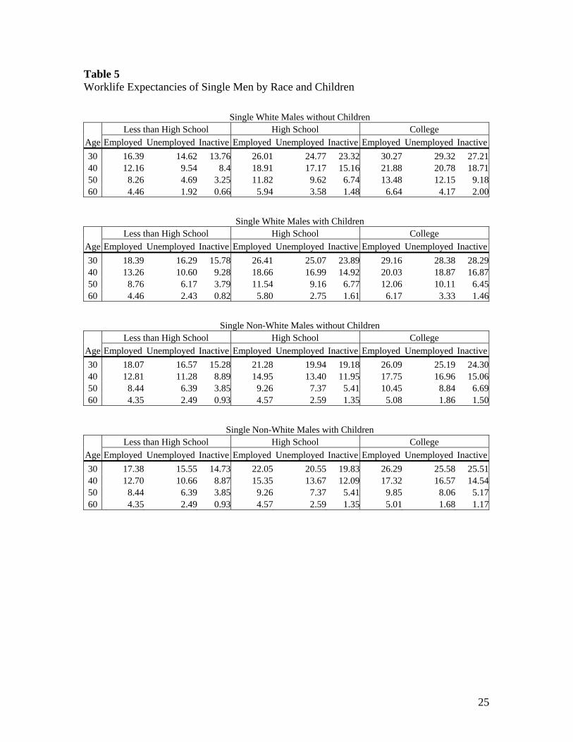
25

Table 5 Worklife Expectancies of Single Men by Race and Children Single White Males without Children Less than High School High School College Age Employed Unemployed Inactive Employed Unemployed Inactive Employed Unemployed Inactive30 16.39 14.62 13.76 26.01 24.77 23.32 30.27 29.32 27.2140 12.16 9.54 8.4 18.91 17.17 15.16 21.88 20.78 18.7150 8.26 4.69 3.25 11.82 9.62 6.74 13.48 12.15 9.1860 4.46 1.92 0.66 5.94 3.58 1.48 6.64 4.17 2.00

Single White Males with Children Less than High School High School College Age Employed Unemployed Inactive Employed Unemployed Inactive Employed Unemployed Inactive30 18.39 16.29 15.78 26.41 25.07 23.89 29.16 28.38 28.2940 13.26 10.60 9.28 18.66 16.99 14.92 20.03 18.87 16.8750 8.76 6.17 3.79 11.54 9.16 6.77 12.06 10.11 6.4560 4.46 2.43 0.82 5.80 2.75 1.61 6.17 3.33 1.46

Single Non-White Males without Children Less than High School High School College Age Employed Unemployed Inactive Employed Unemployed Inactive Employed Unemployed Inactive30 18.07 16.57 15.28 21.28 19.94 19.18 26.09 25.19 24.3040 12.81 11.28 8.89 14.95 13.40 11.95 17.75 16.96 15.0650 8.44 6.39 3.85 9.26 7.37 5.41 10.45 8.84 6.6960 4.35 2.49 0.93 4.57 2.59 1.35 5.08 1.86 1.50

Single Non-White Males with Children Less than High School High School College Age Employed Unemployed Inactive Employed Unemployed Inactive Employed Unemployed Inactive30 17.38 15.55 14.73 22.05 20.55 19.83 26.29 25.58 25.5140 12.70 10.66 8.87 15.35 13.67 12.09 17.32 16.57 14.5450 8.44 6.39 3.85 9.26 7.37 5.41 9.85 8.06 5.1760 4.35 2.49 0.93 4.57 2.59 1.35 5.01 1.68 1.17

26

Table 6 Worklife Expectancies of Married Men by Race and Children Married White Males without Children Less than High School High School College Age Employed Unemployed Inactive Employed Unemployed Inactive Employed Unemployed Inactive30 22.85 21.29 19.37 28.70 27.75 26.17 31.42 30.53 29.6840 15.54 13.68 10.59 20.00 18.85 16.54 22.26 21.30 19.7250 9.44 7.05 4.08 12.04 10.35 7.55 13.67 12.58 9.7360 4.40 2.61 0.84 5.54 3.24 1.84 6.50 4.87 2.45

Married White Males with Children Less than High School High School College Age Employed Unemployed Inactive Employed Unemployed Inactive Employed Unemployed Inactive30 22.48 20.63 19.24 29.01 27.98 26.53 31.14 30.46 30.4340 15.48 13.03 10.70 20.17 19.00 16.62 21.81 21.00 19.6550 9.44 7.05 4.08 12.04 10.35 7.55 13.21 12.01 7.8560 4.40 2.61 0.84 5.54 3.24 1.84 6.41 4.71 1.85

Married Non-White Males without Children Less than High School High School College Age Employed Unemployed Inactive Employed Unemployed Inactive Employed Unemployed Inactive30 21.79 20.42 18.47 25.07 23.87 22.71 28.96 28.15 27.3240 14.82 13.48 10.41 16.99 15.73 13.81 19.96 19.29 17.4550 9.09 7.28 4.33 9.89 8.47 6.08 11.75 10.63 8.0960 4.32 2.74 1.01 4.41 2.99 1.52 5.35 2.61 1.98

Married Non-White Males with Children Less than High School High School College Age Employed Unemployed Inactive Employed Unemployed Inactive Employed Unemployed Inactive30 21.45 19.81 18.31 25.60 24.35 23.23 28.83 28.18 28.1640 14.80 12.98 10.45 17.26 15.94 13.93 19.53 18.91 17.5750 9.09 7.28 4.33 9.89 8.47 6.08 11.21 9.98 6.6360 4.32 2.74 1.01 4.41 2.99 1.52 5.26 2.37 1.55