Embed Size (px)
Citation preview
Volume 124, Article No. 124016 (2019) https://doi.org/10.6028/jres.124.016
Journal of Research of the National Institute of Standards and Technology
1
How to cite this article: Yang JC (2019) Detailed Derivations of Formulas for Heat Release Rate
Calculations Revisited: A Pedagogical and Systematic Approach. J Res Natl Inst Stan 124:124016. https://doi.org/10.6028/jres.124.016
Detailed Derivations of Formulas for Heat Release Rate Calculations Revisited: A Pedagogical and Systematic Approach
Jiann C. Yang National Institute of Standards and Technology, Gaithersburg, MD 20899 USA [email protected] The derivations of the formulas for heat release rate calculations are revisited based on the oxygen consumption principle. A systematic, structured, and pedagogical approach to formulate the problem and derive the generalized formulas with fewer assumptions is used. The operation of oxygen consumption calorimetry is treated as a chemical flow process, the problem is formulated in matrix notation, and the associated material balances using the tie component concept commonly used in chemical engineering practices are solved. The derivation procedure described is intuitive and easy to follow. Inclusion of other chemical species in the measurements and calculations can be easily implemented using the generalized framework developed here. Key words: fire measurement; heat release rate; oxygen consumption calorimetry. Accepted: May 7, 2019 Published: June 24, 2019 https://doi.org/10.6028/jres.124.016
Glossary Symbol Units Description 𝐴𝐴L m2 cross-sectional area of exhaust duct E J/kg heat released per unit amount of oxygen consumed (= 13.1 × 10⁶ J/kg O2) 𝑘𝑘1, 𝑘𝑘2 proportional constant (≪ 1) M kg/mol molecular weight n mol/s material flow rate 𝑛𝑛�T,L mol/s total material flow rate in L-stream with tracer p Pa pressure 𝑝𝑝vap Pa vapor pressure 𝑞𝑞 W heat release rate RH relative humidity (%) S combustion product species T K temperature 𝑣𝑣L m/s gas velocity in the exhaust duct y mol/mol amount-of-substance fraction α expansion factor, defined in Eq. (15)
Volume 124, Article No. 124016 (2019) https://doi.org/10.6028/jres.124.016
Journal of Research of the National Institute of Standards and Technology
2 https://doi.org/10.6028/jres.124.016
β ratio of amount of substance of combustion products formed to that of oxygen consumed, defined in Eq. (12)
ν stoichiometric coefficient ρ mol/m3 density 𝜙𝜙 oxygen depletion factor, defined in Eq. (2)
Subscript A pertaining to A-stream (to analyzers) CO carbon monoxide CO2 carbon dioxide D pertaining to D-stream (to stack) E pertaining to E-stream (entering stream) fuel fuel H2O water i combustion product species i (= 1, 2,…, m) L pertaining to L-stream (leaving stream) m total number of combustion product species N2 nitrogen rxn reacted S pertaining to S-stream (sampling stream) tr tracer gas T total W pertaining to W-stream (water analyzer) Superscript * background (no fire under collection hood) 1. Introduction
Heat release rate, defined as the amount of energy released by a burning material per unit time, is
considered to be the single most important parameter required to characterize the intensity and size of a fire and other fire hazards [1]. The determination of heat release rate can be straightforward if the effective heat of combustion and the burning rate of the tested material are both known. Then, the heat release rate is simply the product of the effective heat of combustion and the burning rate. However, the effective heats of combustion for most materials used in fire tests are generally not known, and measuring burning rates of materials in large-scale fire tests proves quite challenging. Other means need to be developed to measure heat release rates. One such technique is oxygen consumption calorimetry.
In 1917, Thornton [2] observed that the heat released per unit amount of oxygen consumed during the complete combustion of a large number of organic gases and liquids was relatively constant. His finding subsequently formed the basis for modern heat release measurements based on the oxygen consumption principle, from bench-scale cone calorimeters [3] to full-scale fire tests [4]. In 1980, Huggett, at the then-NBS (National Bureau of Standards), expanded Thornton’s work by including typical fuels commonly encountered in fires in his study and recommended an average value of 13.1 MJ of heat released per kilogram of O2 consumed for all fuels with a ± 5 % variation [5]. In 1982, Parker published his seminal work on a detailed derivation of a set of formulas that could be used for heat release calculations using the oxygen consumption principle in an NBS publication [6] and later published a different version of the derivation in Ref. [7]. Janssens [8] revisited the derivations using mass basis instead of the volumetric basis
Volume 124, Article No. 124016 (2019) https://doi.org/10.6028/jres.124.016
Journal of Research of the National Institute of Standards and Technology
3 https://doi.org/10.6028/jres.124.016
used by Parker [6, 7]. Janssens and Parker also summarized the formulas in a chapter of a handbook [9]. Brohez et al. [10] modified the heat release rate formulas for sooty fires. More recently, Chow and Han [11] also presented formulas including soot as an additional species.
The derivations of the formulas in the literature [8, 10, 11] followed essentially the same procedure developed by Parker [6, 7], with little variance. Although the derivations carried out by Parker [6, 7] and others [8, 10, 11] were comprehensive, the approach did not appear to be structured and systematic, and the line of reasoning sometimes was not intuitive. Filling in some of the missing intermediate steps in the derivations was not effortless and required some thinking and assumed knowledge. The use of cumbersome nomenclature, and a myriad of subscripts, superscripts, and super-superscripts, also burdened the readers. Without a complete appreciation for the subtleties involved in the derivation of these equations and the underlying assumptions, incorrect use of the equations or typographical errors introduced inadvertently during transcription of the equations from the literature sources would hardly be noticed by the users, as evidenced by the survey conducted by Lattimer and Beitel [12] on the standard test methods that used the oxygen consumption principle to calculate heat release rates. Of the 17 domestic, foreign, and international standards they reviewed and examined, 12 were identified to have various typographical errors, resulting in 22 incorrect equations in all, and the misprints were found to propagate from standard to standard, most likely attributed to cut-and-paste processes and the poor notations used.
It is necessary to seek a more systematic treatment than those previously presented in the literature. This work is intended to provide a clear and detailed description of the derivations of the formulas used in heat release rate calculations and to make the discussion as general as possible in a consistent and unified manner without introducing additional complexity. The approach presented here is different in many respects from the literature. First, a structured, step-by-step, and pedagogical approach was adopted. For completeness and clarity, this unavoidably led to some of the derivation procedure appearing repetitious in the following discussion. Second, the use of chemical engineering process flow diagrams to illustrate the basic engineering principles and to facilitate the formulation of the necessary material balances was made. Third, matrix representations that enabled the formulations of the species material balances in a very compact and convenient form for presentation, record keeping, and problem solving were used [13]. Fourth, symbols with conventions that are instinctive, self-explanatory, and unambiguous were used. A set of generalized equations with few assumptions was methodically derived and then the equations were simplified under conditions generally encountered in small-scale and large-scale fire tests. Equations are expressed on amount-of-substance basis consistent with practices commonly used in stoichiometric calculations and material balances with chemical reactions.
2. Heat Release Rate Measurements
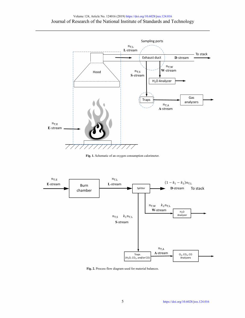
Figure 1 shows a schematic of a typical oxygen consumption calorimeter used to measure heat release
rates. It consists of a hood under which the material of interest is burned to determine its heat release rates. All of the combustion products and the entrained air from the surroundings are drawn into the collection hood. The combustion products are sampled in the exhaust duct, and the concentrations of selected major combustion products as well as oxygen are measured after other combustion products that are not to be measured are removed by the traps. In some of the setups, a provision for the measurement of water vapor concentration in the L-stream is also employed. The three dotted-line demarcations signify the three systems under consideration. The single E-stream representation in Fig. 1 is a simplification; air is entrained from all sides into the burn chamber.
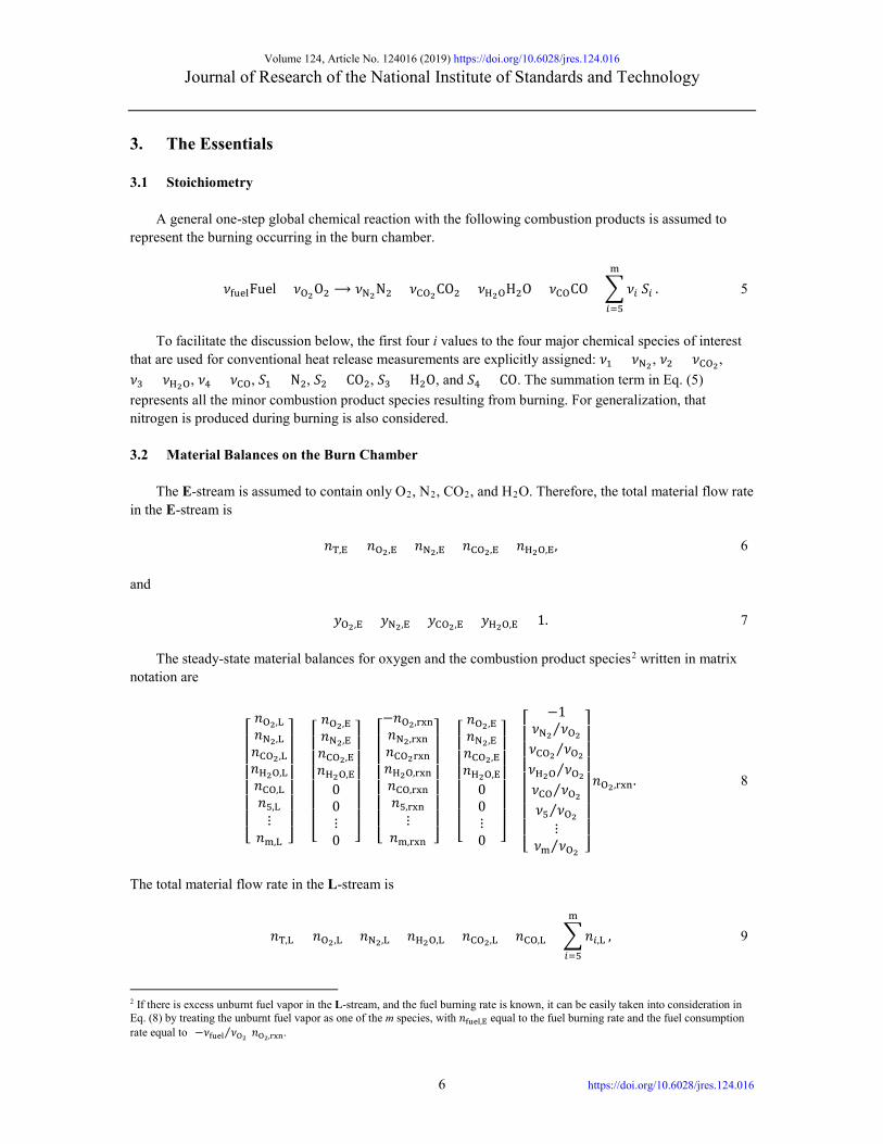
Figure 2 is a simplified process flow diagram representing the oxygen consumption calorimeter in Fig. 1 and the total attendant material streams for the material balances essential to the calculation of the heat release rate. Our focus will be formulating the necessary material balances on the burn chamber, the splitter, and the traps. The splitter, which divides a single input stream (the L-stream) into two or more output streams (the S-stream and the D-stream) with the same composition [14], is used to represent the
Volume 124, Article No. 124016 (2019) https://doi.org/10.6028/jres.124.016
Journal of Research of the National Institute of Standards and Technology
4 https://doi.org/10.6028/jres.124.016
sampling process in the exhaust duct. The traps could be viewed as a separator, which separates or removes one or more components from the incoming S-stream before exiting as the A-stream with fewer components [14]. The components that are not removed by the separator are termed tie components in the S-stream and the A-stream. A tie component is defined as material that goes from one stream into another without changing in any respect or having like material added to it or lost from it [14]. The concept and identification of tie components, which are used extensively in material balance calculations in chemical engineering processes, will provide a very straightforward, convenient, and systematic procedure with which to formulate the equations needed for heat release rate calculations and will greatly facilitate solving the material balances. In the following discussion, it should be noted that the concentrations in the A-stream and the W-stream are measured and considered known. Simply put, the essence of the formulation of heat release calculations is to express the conditions in the E-stream and the L-stream in terms of those in the A-stream and the W-stream. The connection is made through the S-stream. The reason to develop the appropriate formulas is that the presence of the traps alters the composition of the S-stream by removing certain species from the S-stream before the gas concentration measurements in the A-stream.1
Based on the oxygen consumption principle, the heat release rate 𝑞𝑞 is defined as
𝑞𝑞 = 𝐸𝐸𝐸𝐸O2𝑛𝑛O2,rxn = 𝐸𝐸𝐸𝐸O2�𝑛𝑛O2,E − 𝑛𝑛O2,L�, (1)
where E = 13.1 × 10⁶ J/kg O2 consumed. Corrections to E can be made to accommodate incomplete combustion and other conditions [6, 7, 10, 11].
The oxygen depleting factor 𝜙𝜙 was defined by Parker [6] as
𝜙𝜙 =𝑛𝑛O2,E − 𝑛𝑛O2,L
𝑛𝑛O2,E=𝑛𝑛O2,rxn
𝑛𝑛O2,E, (2)
and
𝜙𝜙 =𝑛𝑛T,E 𝑦𝑦O2,E − 𝑛𝑛T,L 𝑦𝑦O2,L
𝑛𝑛T,E 𝑦𝑦O2,E= 1 −
𝑛𝑛T,L 𝑦𝑦O2,L
𝑛𝑛T,E 𝑦𝑦O2,E. (3)
Note that 𝜙𝜙 is equivalent to the term conversion of a reactant, used in chemical reaction engineering [15], where the reactant is oxygen (not fuel) in this case. The conversion of a reactant in a chemical reacting flow system is simply defined as the amount of a reactant reacted or consumed divided by the amount of the reactant fed to the system.
Using the definition of 𝜙𝜙, Eq. (1) can be rewritten as
𝑞𝑞 = 𝐸𝐸𝐸𝐸O2𝑛𝑛O2,E𝜙𝜙 = 𝐸𝐸𝐸𝐸O2𝑦𝑦O2,E 𝑛𝑛T,E𝜙𝜙. (4) If 𝑦𝑦O2,E, 𝑛𝑛T,E, and 𝜙𝜙 are known, the calculation of 𝑞𝑞 is very straightforward using Eq. (4). However,
measuring 𝑛𝑛T,E proves to be difficult for an open system used in fire testing. One needs to come up with a means to bypass the use of 𝑛𝑛T,E in the calculations of 𝑞𝑞 and to relate it to 𝑛𝑛T,L, which can be easily measured in the exhaust duct. What follows will be the discussion on how these three parameters (𝑦𝑦O2,E, 𝑛𝑛T,E, and 𝜙𝜙) can be obtained from a set of formulas derived using material balances and various gas measurement schemes commonly used in fire tests.
1 If no traps were present and oxygen concentration were to be measured hypothetically without the traps, the formulas derived herein for various gas measurement schemes would no longer be required because the species concentrations in the L-stream, in the S-stream, and in the A-stream would all be identical.
Volume 124, Article No. 124016 (2019) https://doi.org/10.6028/jres.124.016
Journal of Research of the National Institute of Standards and Technology
5 https://doi.org/10.6028/jres.124.016
Fig. 1. Schematic of an oxygen consumption calorimeter.
Fig. 2. Process flow diagram used for material balances.
E-stream
A-stream
Hood
Exhaust duct
L-stream
S-stream
Gas analyzersTraps
𝑛𝑛T,E
𝑛𝑛T,L
𝑛𝑛T,S
𝑛𝑛T,A
D-stream
W-stream𝑛𝑛T,W
H2O Analyzer
To stack
Sampling ports
O2, CO2, COAnalyzers
E-stream L-stream
S-stream
A-stream
SplitterBurn
chamber
1 − 𝑘𝑘1 − 𝑘𝑘2 𝑛𝑛T,L
𝑛𝑛T,S = 𝑘𝑘1𝑛𝑛T,L
Traps(H2O, CO2, and/or CO)
𝑛𝑛T,L𝑛𝑛T,E
𝑛𝑛T,A
To stackD-stream
H2OAnalyzer
W-stream𝑛𝑛T,W = 𝑘𝑘2𝑛𝑛T,L
Volume 124, Article No. 124016 (2019) https://doi.org/10.6028/jres.124.016
Journal of Research of the National Institute of Standards and Technology
6 https://doi.org/10.6028/jres.124.016
3. The Essentials
3.1 Stoichiometry A general one-step global chemical reaction with the following combustion products is assumed to
represent the burning occurring in the burn chamber.
𝜈𝜈fuelFuel + 𝜈𝜈O2O2 ⟶ 𝜈𝜈N2N2 + 𝜈𝜈CO2CO2 + 𝜈𝜈H2OH2O + 𝜈𝜈COCO + �𝜈𝜈𝑖𝑖 𝑆𝑆𝑖𝑖
m
𝑖𝑖=5
. (5)
To facilitate the discussion below, the first four i values to the four major chemical species of interest
that are used for conventional heat release measurements are explicitly assigned: 𝜈𝜈1 = 𝜈𝜈N2 , 𝜈𝜈2 = 𝜈𝜈CO2, 𝜈𝜈3 = 𝜈𝜈H2O, 𝜈𝜈4 = 𝜈𝜈CO, 𝑆𝑆1 = N2, 𝑆𝑆2 = CO2, 𝑆𝑆3 = H2O, and 𝑆𝑆4 = CO. The summation term in Eq. (5) represents all the minor combustion product species resulting from burning. For generalization, that nitrogen is produced during burning is also considered.
3.2 Material Balances on the Burn Chamber
The E-stream is assumed to contain only O2, N2, CO2, and H2O. Therefore, the total material flow rate
in the E-stream is
𝑛𝑛T,E = 𝑛𝑛O2,E + 𝑛𝑛N2,E + 𝑛𝑛CO2,E + 𝑛𝑛H2O,E, (6) and
𝑦𝑦O2,E + 𝑦𝑦N2,E + 𝑦𝑦CO2,E + 𝑦𝑦H2O,E = 1. (7) The steady-state material balances for oxygen and the combustion product species2 written in matrix
notation are
⎣⎢⎢⎢⎢⎢⎢⎡𝑛𝑛O2,L𝑛𝑛N2,L𝑛𝑛CO2,L𝑛𝑛H2O,L𝑛𝑛CO,L𝑛𝑛5,L⋮
𝑛𝑛m,L ⎦⎥⎥⎥⎥⎥⎥⎤
=
⎣⎢⎢⎢⎢⎢⎢⎡𝑛𝑛O2,E𝑛𝑛N2,E𝑛𝑛CO2,E𝑛𝑛H2O,E
00⋮0 ⎦
⎥⎥⎥⎥⎥⎥⎤
+
⎣⎢⎢⎢⎢⎢⎢⎡−𝑛𝑛O2,rxn𝑛𝑛N2,rxn𝑛𝑛CO2rxn𝑛𝑛H2O,rxn𝑛𝑛CO,rxn𝑛𝑛5,rxn⋮
𝑛𝑛m,rxn ⎦⎥⎥⎥⎥⎥⎥⎤
=
⎣⎢⎢⎢⎢⎢⎢⎡𝑛𝑛O2,E𝑛𝑛N2,E𝑛𝑛CO2,E𝑛𝑛H2O,E
00⋮0 ⎦
⎥⎥⎥⎥⎥⎥⎤
+
⎣⎢⎢⎢⎢⎢⎢⎢⎡
−1𝜈𝜈N2 𝜈𝜈O2⁄𝜈𝜈CO2 𝜈𝜈O2⁄𝜈𝜈H2O 𝜈𝜈O2⁄𝜈𝜈CO 𝜈𝜈O2⁄𝜈𝜈5 𝜈𝜈O2⁄
⋮𝜈𝜈m 𝜈𝜈O2⁄ ⎦
⎥⎥⎥⎥⎥⎥⎥⎤
𝑛𝑛O2,rxn. (8)
The total material flow rate in the L-stream is
𝑛𝑛T,L = 𝑛𝑛O2,L + 𝑛𝑛N2,L + 𝑛𝑛H2O,L + 𝑛𝑛CO2,L + 𝑛𝑛CO,L + �𝑛𝑛𝑖𝑖,L
m
𝑖𝑖=5
, (9)
2 If there is excess unburnt fuel vapor in the L-stream, and the fuel burning rate is known, it can be easily taken into consideration in Eq. (8) by treating the unburnt fuel vapor as one of the m species, with 𝑛𝑛fuel,E equal to the fuel burning rate and the fuel consumption rate equal to (−𝜈𝜈fuel 𝜈𝜈O2)𝑛𝑛O2,rxn⁄ .
Volume 124, Article No. 124016 (2019) https://doi.org/10.6028/jres.124.016
Journal of Research of the National Institute of Standards and Technology
7 https://doi.org/10.6028/jres.124.016
and
𝑦𝑦O2,L + 𝑦𝑦N2,L + 𝑦𝑦H2O,L + 𝑦𝑦CO2,L + 𝑦𝑦CO,L + �𝑦𝑦𝑖𝑖 ,L
m
𝑖𝑖=5
= 1. (10)
Substituting the corresponding matrix elements in Eq. (8) into Eq. (9) and simplifying using Eq. (6),
one obtains
𝑛𝑛T,L = 𝑛𝑛T,E + �𝜈𝜈N2𝜈𝜈O2
+𝜈𝜈H2O
𝜈𝜈O2+𝜈𝜈CO2𝜈𝜈O2
+𝜈𝜈CO𝜈𝜈O2
+ �𝜈𝜈𝑖𝑖𝜈𝜈O2
m
𝑖𝑖=5
− 1� �𝑦𝑦O2,E 𝑛𝑛T,E − 𝑦𝑦O2,L 𝑛𝑛T,L�. (11)
Define
𝛽𝛽 = �𝜈𝜈N2𝜈𝜈O2
+𝜈𝜈H2O
𝜈𝜈O2+𝜈𝜈CO2𝜈𝜈O2
+𝜈𝜈CO𝜈𝜈O2
+ �𝜈𝜈𝑖𝑖𝜈𝜈O2
m
𝑖𝑖=5
� . (12)
This definition is analogous to that defined by Parker [6]. Using Eq. (12), Eq. (11) can be rewritten as
𝑛𝑛T,L
𝑛𝑛T,E=
1 + (𝛽𝛽 − 1)𝑦𝑦O2,E
1 + (𝛽𝛽 − 1)𝑦𝑦O2,L. (13)
Using the definition of 𝜙𝜙, Eq. (13) can be expressed in terms of 𝜙𝜙 as
𝑛𝑛T,L
𝑛𝑛T,E= 1 + (𝛽𝛽 − 1)𝜙𝜙 𝑦𝑦O2,E. (14)
Following Parker [6], the expansion factor 𝛼𝛼 can be defined as the ratio of 𝑛𝑛T,L to 𝑛𝑛T,E with 𝑛𝑛T,L
completely depleted of its oxygen (i.e., 𝑦𝑦O2,L = 0). From Eq. (13) with 𝑦𝑦O2,L = 0, one obtains
𝛼𝛼 =�𝑛𝑛T,L�𝑦𝑦O2,L=0
𝑛𝑛T,E=
1 + (𝛽𝛽 − 1)𝑦𝑦O2,E
1 + (𝛽𝛽 − 1)𝑦𝑦O2,L= 1 + (𝛽𝛽 − 1)𝑦𝑦O2,E. (15)
Substituting Eq. (15) into Eq. (14),
𝑛𝑛T,E
𝑛𝑛T,L=
11 + (𝛼𝛼 − 1)𝜙𝜙
. (16)
Therefore, the material balances on the burner chamber provide a relationship between 𝑛𝑛T,E and 𝑛𝑛T,L in
terms of 𝛽𝛽 and 𝜙𝜙 [Eq. (14)] or 𝛼𝛼 and 𝜙𝜙 [Eq. (16)]. If water vapor is measured in the L-stream, then 𝛽𝛽 can be obtained from the procedure described in Appendix B; otherwise, a nominal value of 1.1 for 𝛼𝛼 is recommended [6], which is approximately the value for methane.
3.3 Material Balances on the Splitter
The splitter signifies the process occurring at the sampling port in the exhaust duct. By the physical nature of sampling, the species concentrations in the L-stream, the S-stream, the W-stream, and the D-stream are the same.
Volume 124, Article No. 124016 (2019) https://doi.org/10.6028/jres.124.016
Journal of Research of the National Institute of Standards and Technology
8 https://doi.org/10.6028/jres.124.016
⎣⎢⎢⎢⎢⎢⎢⎢⎡𝑦𝑦O2,S𝑦𝑦N2,S𝑦𝑦CO2,S𝑦𝑦H2O,S𝑦𝑦CO,S𝑦𝑦5,S𝑦𝑦6,S⋮
𝑦𝑦m,S ⎦⎥⎥⎥⎥⎥⎥⎥⎤
=
⎣⎢⎢⎢⎢⎢⎢⎢⎡𝑦𝑦O2,L𝑦𝑦N2,L𝑦𝑦CO2,L𝑦𝑦H2O,L𝑦𝑦CO,L𝑦𝑦5,L𝑦𝑦6,L⋮
𝑦𝑦m,L ⎦⎥⎥⎥⎥⎥⎥⎥⎤
=
⎣⎢⎢⎢⎢⎢⎢⎢⎡𝑦𝑦O2,W𝑦𝑦N2,W𝑦𝑦CO2,W𝑦𝑦H2O,W𝑦𝑦CO,W𝑦𝑦5,W𝑦𝑦6,W⋮
𝑦𝑦m,W ⎦⎥⎥⎥⎥⎥⎥⎥⎤
=
⎣⎢⎢⎢⎢⎢⎢⎢⎡𝑦𝑦O2,D𝑦𝑦N2,D𝑦𝑦CO2,D𝑦𝑦H2O,D𝑦𝑦CO,D𝑦𝑦5,D𝑦𝑦6,D⋮
𝑦𝑦m,D ⎦⎥⎥⎥⎥⎥⎥⎥⎤
. (17)
Then,
1𝑛𝑛T,S
⎣⎢⎢⎢⎢⎢⎢⎢⎡𝑛𝑛O2,S𝑛𝑛N2,S𝑛𝑛CO2,S𝑛𝑛H2O,S𝑛𝑛CO,S𝑛𝑛5,S𝑛𝑛6,S⋮
𝑛𝑛m,S ⎦⎥⎥⎥⎥⎥⎥⎥⎤
=1𝑛𝑛T,L
⎣⎢⎢⎢⎢⎢⎢⎢⎡𝑛𝑛O2,L𝑛𝑛N2,L𝑛𝑛CO2,L𝑛𝑛H2O,L𝑛𝑛CO,L𝑛𝑛5,L𝑛𝑛6,L⋮
𝑛𝑛m,L ⎦⎥⎥⎥⎥⎥⎥⎥⎤
=1
𝑛𝑛T,W
⎣⎢⎢⎢⎢⎢⎢⎢⎡𝑛𝑛O2,W𝑛𝑛N2,W𝑛𝑛CO2,W𝑛𝑛H2O,W𝑛𝑛CO,W𝑛𝑛5,W𝑛𝑛6,W⋮
𝑛𝑛m,W ⎦⎥⎥⎥⎥⎥⎥⎥⎤
=1𝑛𝑛T,D
⎣⎢⎢⎢⎢⎢⎢⎢⎡𝑛𝑛O2,D𝑛𝑛N2,D𝑛𝑛CO2,D𝑛𝑛H2O,D𝑛𝑛CO,D𝑛𝑛5,D𝑛𝑛6,D⋮
𝑛𝑛m,D ⎦⎥⎥⎥⎥⎥⎥⎥⎤
and
⎣⎢⎢⎢⎢⎢⎢⎢⎡𝑛𝑛O2,S𝑛𝑛N2,S𝑛𝑛CO2,S𝑛𝑛H2O,S𝑛𝑛CO,S𝑛𝑛5,S𝑛𝑛6,S⋮
𝑛𝑛m,S ⎦⎥⎥⎥⎥⎥⎥⎥⎤
=𝑛𝑛T,S
𝑛𝑛T,L
⎣⎢⎢⎢⎢⎢⎢⎢⎡𝑛𝑛O2,L𝑛𝑛N2,L𝑛𝑛CO2,L𝑛𝑛H2O,L𝑛𝑛CO,L𝑛𝑛5,L𝑛𝑛6,L⋮
𝑛𝑛m,L ⎦⎥⎥⎥⎥⎥⎥⎥⎤
=𝑛𝑛T,S
𝑛𝑛T,W
⎣⎢⎢⎢⎢⎢⎢⎢⎡𝑛𝑛O2,W𝑛𝑛N2,W𝑛𝑛CO2,W𝑛𝑛H2O,W𝑛𝑛CO,W𝑛𝑛5,W𝑛𝑛6,W⋮
𝑛𝑛m,W ⎦⎥⎥⎥⎥⎥⎥⎥⎤
=𝑛𝑛T,S
𝑛𝑛T,D
⎣⎢⎢⎢⎢⎢⎢⎢⎡𝑛𝑛O2,D𝑛𝑛N2,D𝑛𝑛CO2,D𝑛𝑛H2O,D𝑛𝑛CO,D𝑛𝑛5,D𝑛𝑛6,D⋮
𝑛𝑛m,D ⎦⎥⎥⎥⎥⎥⎥⎥⎤
. (18)
Since 𝑛𝑛T,L = 𝑛𝑛T,S + 𝑛𝑛T,W + 𝑛𝑛T,D, Eq. (18) becomes
⎣⎢⎢⎢⎢⎢⎢⎢⎡𝑛𝑛O2,S𝑛𝑛N2,S𝑛𝑛CO2,S𝑛𝑛H2O,S𝑛𝑛CO,S𝑛𝑛5,S𝑛𝑛6,S⋮
𝑛𝑛m,S ⎦⎥⎥⎥⎥⎥⎥⎥⎤
=𝑛𝑛T,S
𝑛𝑛T,L
⎣⎢⎢⎢⎢⎢⎢⎢⎡𝑛𝑛O2,L𝑛𝑛N2,L𝑛𝑛CO2,L𝑛𝑛H2O,L𝑛𝑛CO,L𝑛𝑛5,L𝑛𝑛6,L⋮
𝑛𝑛m,L ⎦⎥⎥⎥⎥⎥⎥⎥⎤
=𝑛𝑛T,S
𝑛𝑛T,W
⎣⎢⎢⎢⎢⎢⎢⎢⎡𝑛𝑛O2,W𝑛𝑛N2,W𝑛𝑛CO2,W𝑛𝑛H2O,W𝑛𝑛CO,W𝑛𝑛5,W𝑛𝑛6,W⋮
𝑛𝑛m,W ⎦⎥⎥⎥⎥⎥⎥⎥⎤
=𝑛𝑛T,S
𝑛𝑛T,L − 𝑛𝑛T,S − 𝑛𝑛T,W
⎣⎢⎢⎢⎢⎢⎢⎢⎡𝑛𝑛O2,D𝑛𝑛N2,D𝑛𝑛CO2,D𝑛𝑛H2O,D𝑛𝑛CO,D𝑛𝑛5,D𝑛𝑛6,D⋮
𝑛𝑛m,D ⎦⎥⎥⎥⎥⎥⎥⎥⎤
. (19)
Define
𝑘𝑘1 =𝑛𝑛T,S
𝑛𝑛T,L, (20)
and
𝑘𝑘2 =𝑛𝑛T,W
𝑛𝑛T,L. (21)
Volume 124, Article No. 124016 (2019) https://doi.org/10.6028/jres.124.016
Journal of Research of the National Institute of Standards and Technology
9 https://doi.org/10.6028/jres.124.016
Equation (19) becomes
⎣⎢⎢⎢⎢⎢⎢⎢⎡𝑛𝑛O2,S𝑛𝑛N2,S𝑛𝑛CO2,S𝑛𝑛H2O,S𝑛𝑛CO,S𝑛𝑛5,S𝑛𝑛6,S⋮
𝑛𝑛m,S ⎦⎥⎥⎥⎥⎥⎥⎥⎤
= 𝑘𝑘1
⎣⎢⎢⎢⎢⎢⎢⎢⎡𝑛𝑛O2,L𝑛𝑛N2,L𝑛𝑛CO2,L𝑛𝑛H2O,L𝑛𝑛CO,L𝑛𝑛5,L𝑛𝑛6,L⋮
𝑛𝑛m,L ⎦⎥⎥⎥⎥⎥⎥⎥⎤
=𝑘𝑘1𝑘𝑘2
⎣⎢⎢⎢⎢⎢⎢⎢⎡𝑛𝑛O2,W𝑛𝑛N2,W𝑛𝑛CO2,W𝑛𝑛H2O,W𝑛𝑛CO,W𝑛𝑛5,W𝑛𝑛6,W⋮
𝑛𝑛m,W ⎦⎥⎥⎥⎥⎥⎥⎥⎤
=𝑘𝑘1
1 − 𝑘𝑘1 − 𝑘𝑘2
⎣⎢⎢⎢⎢⎢⎢⎢⎡𝑛𝑛O2,D𝑛𝑛N2,D𝑛𝑛CO2,D𝑛𝑛H2O,D𝑛𝑛CO,D𝑛𝑛5,D𝑛𝑛6,D⋮
𝑛𝑛m,D ⎦⎥⎥⎥⎥⎥⎥⎥⎤
. (22)
For gas sampling, 𝑘𝑘1 ≪ 1, 𝑘𝑘2 ≪ 1, and 𝑛𝑛T,S (the S-stream) and 𝑛𝑛T,W (the W-stream) are only a very small fraction of 𝑛𝑛T,L (the L-stream), and 𝑛𝑛T,D ≫ 𝑛𝑛T,S + 𝑛𝑛T,W.
3.4 Material Balances on the Traps
In most oxygen-consumption calorimeters used to measure heat release rates, only the major species,
i.e., O2, CO2, H2O, and/or CO, are measured by the gas analyzers. The discussion below assumes dry-basis measurements for O2, CO2, and CO. In most fire-test applications, one of the following four specific gas measurement schemes (schemes A, B, C, and D) will typically be employed, depending on the species that is/are removed by the traps.
3.4.1 Scheme A (O2 Measured)
In this case, H2O, CO2, and CO are removed by the traps, and O2, N2, and Si (i = 5…m) are the tie
components in the S-stream and the A-stream. One has
𝑛𝑛T,W = 0,
𝑛𝑛T,A = 𝑛𝑛O2,A + 𝑛𝑛N2,A + �𝑛𝑛𝑖𝑖,A
m
𝑖𝑖=5
, (23)
𝑛𝑛H2O,A = 𝑛𝑛CO2,A = 𝑛𝑛CO,A = 0,
𝑦𝑦O2,A + 𝑦𝑦N2,A + �𝑦𝑦𝑖𝑖 ,A
m
𝑖𝑖=5
= 1, (24)
and
⎣⎢⎢⎢⎡𝑛𝑛O2,S𝑛𝑛N2,S𝑛𝑛5,S⋮
𝑛𝑛m,S ⎦⎥⎥⎥⎤
=
⎣⎢⎢⎢⎡𝑛𝑛O2,A𝑛𝑛N2,A𝑛𝑛5,A⋮
𝑛𝑛m,A ⎦⎥⎥⎥⎤
. (25)
Using Eq. (22), Eq. (25) becomes
Volume 124, Article No. 124016 (2019) https://doi.org/10.6028/jres.124.016
Journal of Research of the National Institute of Standards and Technology
10 https://doi.org/10.6028/jres.124.016
⎣⎢⎢⎢⎡𝑛𝑛O2,L𝑛𝑛N2,L𝑛𝑛5,L⋮
𝑛𝑛m,L ⎦⎥⎥⎥⎤
= 1𝑘𝑘1
⎣⎢⎢⎢⎡𝑛𝑛O2,A𝑛𝑛N2,A𝑛𝑛5,A⋮
𝑛𝑛m,A ⎦⎥⎥⎥⎤,
and
𝑛𝑛T,L
⎣⎢⎢⎢⎡𝑦𝑦O2,L𝑦𝑦N2,L𝑦𝑦5,L⋮
𝑦𝑦m,L ⎦⎥⎥⎥⎤
=𝑛𝑛T,A
𝑘𝑘1⎣⎢⎢⎢⎡𝑦𝑦O2,A𝑦𝑦N2,A𝑦𝑦5,A⋮
𝑦𝑦m,A ⎦⎥⎥⎥⎤.
Using Eq. (23),
⎣⎢⎢⎢⎡𝑦𝑦O2,L𝑦𝑦N2,L𝑦𝑦5,L⋮
𝑦𝑦m,L ⎦⎥⎥⎥⎤
=𝑛𝑛O2,A + 𝑛𝑛N2,A + � 𝑛𝑛𝑖𝑖,A
m𝑖𝑖=5
𝑘𝑘1 𝑛𝑛T,L
⎣⎢⎢⎢⎡𝑦𝑦O2,A𝑦𝑦N2,A𝑦𝑦5,A⋮
𝑦𝑦m,A ⎦⎥⎥⎥⎤.
Using Eq. (22) and Eq. (25), it can be easily shown that
⎣⎢⎢⎢⎡𝑦𝑦O2,L𝑦𝑦N2,L𝑦𝑦5,L⋮
𝑦𝑦m,L ⎦⎥⎥⎥⎤
= �𝑦𝑦O2,L + 𝑦𝑦N2,L + �𝑦𝑦𝑖𝑖,L
m
𝑖𝑖=5
�
⎣⎢⎢⎢⎡𝑦𝑦O2,A𝑦𝑦N2,A𝑦𝑦5,A⋮
𝑦𝑦m,A ⎦⎥⎥⎥⎤
. (26)
Using Eq. (10), Eq. (26) can be expressed as
⎣⎢⎢⎢⎡𝑦𝑦O2,L𝑦𝑦N2,L𝑦𝑦5,L⋮
𝑦𝑦m,L ⎦⎥⎥⎥⎤
= �1 − 𝑦𝑦H2O,L − 𝑦𝑦CO2,L − 𝑦𝑦CO,L�
⎣⎢⎢⎢⎡𝑦𝑦O2,A𝑦𝑦N2,A𝑦𝑦5,A⋮
𝑦𝑦m,A ⎦⎥⎥⎥⎤
. (27)
Equation (26) can be rewritten as
⎣⎢⎢⎢⎢⎡�1 − 𝑦𝑦O2,A� −𝑦𝑦O2,A −𝑦𝑦O2,A −𝑦𝑦O2,A −𝑦𝑦O2,A ⋯ −𝑦𝑦O2,A
−𝑦𝑦N2,A �1 − 𝑦𝑦N2,A� −𝑦𝑦N2,A −𝑦𝑦N2,A −𝑦𝑦N2,A ⋯ −𝑦𝑦N2,A
−𝑦𝑦5,A −𝑦𝑦5,A �1 − 𝑦𝑦5,A� −𝑦𝑦5,A −𝑦𝑦5,A ⋯ −𝑦𝑦5,A⋮ ⋮ ⋮ ⋮ ⋮ ⋱ ⋮
−𝑦𝑦m,A −𝑦𝑦m,A −𝑦𝑦m,A −𝑦𝑦m,A −𝑦𝑦m,A ⋯ �1 − 𝑦𝑦m,A�⎦⎥⎥⎥⎥⎤
⎣⎢⎢⎢⎡𝑦𝑦O2,L𝑦𝑦N2,L𝑦𝑦5,L⋮
𝑦𝑦m,L ⎦⎥⎥⎥⎤
=
⎣⎢⎢⎢⎡000⋮0⎦⎥⎥⎥⎤
. (28)
The above (m − 2) × (m − 2) coefficient matrix has a rank of (m − 3); therefore, only (m − 3) equations
are independent [16]. One corresponding row from the three matrices in Eq. (28) may be omitted and only the matrices with the rows associated with 𝑦𝑦O2,L, and 𝑦𝑦5,L ⋯𝑦𝑦m,L is considered. Equation (28) can be manipulated and reduced to the following form.
Volume 124, Article No. 124016 (2019) https://doi.org/10.6028/jres.124.016
Journal of Research of the National Institute of Standards and Technology
11 https://doi.org/10.6028/jres.124.016
⎣⎢⎢⎢⎡�1 − 𝑦𝑦O2,A� −𝑦𝑦O2,A ⋯ −𝑦𝑦O2,A
−𝑦𝑦5,A �1 − 𝑦𝑦5,A� ⋯ −𝑦𝑦5,A⋮ ⋮ ⋱ ⋮
−𝑦𝑦m,A −𝑦𝑦m,A ⋯ �1 − 𝑦𝑦m,A�⎦⎥⎥⎥⎤�
𝑦𝑦O2,L𝑦𝑦5,L⋮
𝑦𝑦m,L
� = �
𝑦𝑦O2,A 𝑦𝑦N2,L𝑦𝑦5,A 𝑦𝑦N2,L
⋮𝑦𝑦m,A 𝑦𝑦N2,L
� . (29)
Solving for 𝑦𝑦O2,L and 𝑦𝑦5,L ⋯𝑦𝑦m,L,
�
𝑦𝑦O2,L𝑦𝑦5,L⋮
𝑦𝑦m,L
� =
⎣⎢⎢⎢⎡�1 − 𝑦𝑦O2,A� −𝑦𝑦O2,A ⋯ −𝑦𝑦O2,A
−𝑦𝑦5,A �1 − 𝑦𝑦5,A� ⋯ −𝑦𝑦5,A⋮ ⋮ ⋱ ⋮
−𝑦𝑦m,A −𝑦𝑦m,A ⋯ �1 − 𝑦𝑦m,A�⎦⎥⎥⎥⎤−1
�
𝑦𝑦O2,A 𝑦𝑦N2,L𝑦𝑦5,A 𝑦𝑦N2,L
⋮𝑦𝑦m,A 𝑦𝑦N2,L
� . (30)
Simplifying by using the inverse of the above matrix given in Appendix A, Eq. (30) becomes
�
𝑦𝑦O2,L𝑦𝑦5,L⋮
𝑦𝑦m,L
� =𝑦𝑦N2,L
�1 − 𝑦𝑦O2,A −� 𝑦𝑦𝑖𝑖,Am𝑖𝑖=5 �
�
𝑦𝑦O2,A 𝑦𝑦5,A⋮
𝑦𝑦m,A
� . (31)
In most fire test applications, the major combustion product species in the L-stream are O2, N2, CO2,
H2O, and CO. It could be assumed that
�𝑦𝑦𝑖𝑖 ,A
m
𝑖𝑖=5
≪ 1. (32)
Therefore, Eq. (31) can be simplified and approximated to
𝑦𝑦O2,L ≅𝑦𝑦N2,L
�1 − 𝑦𝑦O2,A�𝑦𝑦O2,A . (33)
3.4.2 Scheme B (O2 and CO2 Measured)
In this case, H2O and CO are removed by the traps, and O2, N2, CO2, and Si (i = 5…m) are the tie
components in the S-stream and the A-stream. Then,
𝑛𝑛T,W = 0,
𝑛𝑛T,A = 𝑛𝑛O2,A + 𝑛𝑛N2,A + 𝑛𝑛CO2,A + �𝑛𝑛𝑖𝑖,A,m
𝑖𝑖=5
(34)
𝑛𝑛H2O,A = 𝑛𝑛CO,A = 0,
𝑦𝑦O2,A + 𝑦𝑦N2,A + 𝑦𝑦CO2,A + �𝑦𝑦𝑖𝑖,A
m
𝑖𝑖=5
= 1, (35)
and
Volume 124, Article No. 124016 (2019) https://doi.org/10.6028/jres.124.016
Journal of Research of the National Institute of Standards and Technology
12 https://doi.org/10.6028/jres.124.016
⎣⎢⎢⎢⎢⎡𝑛𝑛O2,S𝑛𝑛N2,S𝑛𝑛CO2,S 𝑛𝑛5,S⋮
𝑛𝑛m,S ⎦⎥⎥⎥⎥⎤
=
⎣⎢⎢⎢⎢⎡𝑛𝑛O2,A𝑛𝑛N2,A𝑛𝑛CO2,A 𝑛𝑛5,A⋮
𝑛𝑛m,A ⎦⎥⎥⎥⎥⎤
= 𝑘𝑘1
⎣⎢⎢⎢⎢⎡𝑛𝑛O2,L𝑛𝑛N2,L𝑛𝑛CO2,L 𝑛𝑛5,L⋮
𝑛𝑛m,L ⎦⎥⎥⎥⎥⎤
.
Following the same procedure described in scheme A, it can be easily shown that
⎣⎢⎢⎢⎢⎡𝑦𝑦O2,L𝑦𝑦N2,L𝑦𝑦CO2,L𝑦𝑦5,L⋮
𝑦𝑦m,L ⎦⎥⎥⎥⎥⎤
= �𝑦𝑦O2,L + 𝑦𝑦N2,L + 𝑦𝑦CO2,L + �𝑦𝑦𝑖𝑖 ,L
m
𝑖𝑖=5
�
⎣⎢⎢⎢⎢⎡𝑦𝑦O2,A𝑦𝑦N2,A𝑦𝑦CO2,A𝑦𝑦5,A⋮
𝑦𝑦m,A ⎦⎥⎥⎥⎥⎤
. (36)
Using Eq. (10), Eq. (36) can be expressed as
⎣⎢⎢⎢⎢⎡𝑦𝑦O2,L𝑦𝑦N2,L𝑦𝑦CO2,L𝑦𝑦5,L⋮
𝑦𝑦m,L ⎦⎥⎥⎥⎥⎤
= �1 − 𝑦𝑦H2O,L − 𝑦𝑦CO,L�
⎣⎢⎢⎢⎢⎡𝑦𝑦O2,A𝑦𝑦N2,A𝑦𝑦CO2,A𝑦𝑦5,A⋮
𝑦𝑦m,A ⎦⎥⎥⎥⎥⎤
. (37)
Equation (36) can be rewritten as
⎣⎢⎢⎢⎢⎢⎡�1 − 𝑦𝑦O2,A� −𝑦𝑦O2,A −𝑦𝑦O2,A −𝑦𝑦O2,A −𝑦𝑦O2,A ⋯ −𝑦𝑦O2,A
−𝑦𝑦N2,A �1 − 𝑦𝑦N2,A� −𝑦𝑦N2,A −𝑦𝑦N2,A −𝑦𝑦N2,A ⋯ −𝑦𝑦N2,A
−𝑦𝑦CO2,A −𝑦𝑦CO2,A (1 − 𝑦𝑦CO2,A) −𝑦𝑦CO2,A −𝑦𝑦CO2,A ⋯ −𝑦𝑦CO2,A
−𝑦𝑦5,A −𝑦𝑦5,A −𝑦𝑦5,A �1 − 𝑦𝑦5,A� −𝑦𝑦5,A ⋯ −𝑦𝑦5,A⋮ ⋮ ⋮ ⋮ ⋮ ⋱ ⋮
−𝑦𝑦m,A −𝑦𝑦m,A −𝑦𝑦m,A −𝑦𝑦m,A −𝑦𝑦m,A ⋯ �1 − 𝑦𝑦m,A�⎦⎥⎥⎥⎥⎥⎤
⎣⎢⎢⎢⎢⎡𝑦𝑦O2,L𝑦𝑦N2,L𝑦𝑦CO2,L𝑦𝑦5,L⋮
𝑦𝑦m,L ⎦⎥⎥⎥⎥⎤
=
⎣⎢⎢⎢⎢⎡0000⋮0⎦⎥⎥⎥⎥⎤
. (38)
The (m − 1) × (m − 1) coefficient matrix has a rank of (m − 2); therefore, only (m − 2) equations are
independent [16]. The matrices with the rows associated with 𝑦𝑦O2,L, 𝑦𝑦CO2,L, and 𝑦𝑦5,L ⋯𝑦𝑦m,L are only considered. Equation (38) can be manipulated and reduced to the following form.
⎣⎢⎢⎢⎢⎡�1 − 𝑦𝑦O2,A� −𝑦𝑦O2,A −𝑦𝑦O2,A −𝑦𝑦O2,A ⋯ −𝑦𝑦O2,A
−𝑦𝑦CO2,A �1 − 𝑦𝑦CO2,A� −𝑦𝑦CO2,A −𝑦𝑦CO2,A ⋯ −𝑦𝑦CO2,A
−𝑦𝑦5,A −𝑦𝑦5,A �1 − 𝑦𝑦5,A� −𝑦𝑦5,A ⋯ −𝑦𝑦5,A⋮ ⋮ ⋮ ⋮ ⋱ ⋮
−𝑦𝑦m,A −𝑦𝑦m,A −𝑦𝑦m,A −𝑦𝑦m,A ⋯ �1 − 𝑦𝑦m,A�⎦⎥⎥⎥⎥⎤
⎣⎢⎢⎢⎡𝑦𝑦O2,L𝑦𝑦CO2,L𝑦𝑦5,L⋮
𝑦𝑦m,L ⎦⎥⎥⎥⎤
=
⎣⎢⎢⎢⎡𝑦𝑦O2,A 𝑦𝑦N2,L𝑦𝑦CO2,A 𝑦𝑦N2,L 𝑦𝑦5,A 𝑦𝑦N2,L
⋮𝑦𝑦m,A 𝑦𝑦N2,L ⎦
⎥⎥⎥⎤
. (39)
Solving for 𝑦𝑦O2,L, 𝑦𝑦CO2,L, and 𝑦𝑦5,L ⋯𝑦𝑦m,L,
Volume 124, Article No. 124016 (2019) https://doi.org/10.6028/jres.124.016
Journal of Research of the National Institute of Standards and Technology
13 https://doi.org/10.6028/jres.124.016
⎣⎢⎢⎢⎡𝑦𝑦O2,L𝑦𝑦CO2,L𝑦𝑦5,L⋮
𝑦𝑦m,L ⎦⎥⎥⎥⎤
=
⎣⎢⎢⎢⎢⎡�1 − 𝑦𝑦O2,A� −𝑦𝑦O2,A −𝑦𝑦O2,A −𝑦𝑦O2,A ⋯ −𝑦𝑦O2,A
−𝑦𝑦CO2,A �1 − 𝑦𝑦CO2,A� −𝑦𝑦CO2,A −𝑦𝑦CO2,A ⋯ −𝑦𝑦CO2,A
−𝑦𝑦5,A −𝑦𝑦5,A �1 − 𝑦𝑦5,A� −𝑦𝑦5,A ⋯ −𝑦𝑦5,A⋮ ⋮ ⋮ ⋮ ⋱ ⋮
−𝑦𝑦m,A −𝑦𝑦m,A −𝑦𝑦m,A −𝑦𝑦m,A ⋯ �1 − 𝑦𝑦m,A�⎦⎥⎥⎥⎥⎤−1
⎣⎢⎢⎢⎡𝑦𝑦O2,A 𝑦𝑦N2,L𝑦𝑦CO2,A 𝑦𝑦N2,L 𝑦𝑦5,A 𝑦𝑦N2,L
⋮𝑦𝑦m,A 𝑦𝑦N2,L ⎦
⎥⎥⎥⎤
. (40)
Simplifying by using the inverse of the above matrix given in Appendix A, Eq. (40) becomes
⎣⎢⎢⎢⎡𝑦𝑦O2,L𝑦𝑦CO2,L𝑦𝑦5,L⋮
𝑦𝑦m,L ⎦⎥⎥⎥⎤
=𝑦𝑦N2,L
�1 − 𝑦𝑦O2,A − 𝑦𝑦CO2,A −� 𝑦𝑦𝑖𝑖 ,Am𝑖𝑖=5 �
⎣⎢⎢⎢⎡𝑦𝑦O2,A𝑦𝑦CO2,A𝑦𝑦5,A⋮
𝑦𝑦m,A ⎦⎥⎥⎥⎤
. (41)
Similar to scheme A, with � 𝑦𝑦𝑖𝑖,A
m𝑖𝑖=5 ≪ 1, Eq. (41) simplifies to the following equation.
�𝑦𝑦O2,L𝑦𝑦CO2,L
� ≅𝑦𝑦N2,L
�1 − 𝑦𝑦O2,A − 𝑦𝑦CO2,A��𝑦𝑦O2,A𝑦𝑦CO2,A
� . (42)
3.4.3 Scheme C (O2, CO2, and CO Measured)
Under this condition, H2O is removed by the traps, and O2, N2, CO2, CO, and Si (i = 5…m) are the tie components in the S-stream and the A-stream. Then,
𝑛𝑛T,W = 0,
𝑛𝑛T,A = 𝑛𝑛O2,A + 𝑛𝑛N2,A + 𝑛𝑛CO2,A + 𝑛𝑛CO,A + �𝑛𝑛𝑖𝑖,A
m
𝑖𝑖=5
, (43)
𝑛𝑛H2O,A = 0,
𝑦𝑦O2,A + 𝑦𝑦N2,A + 𝑦𝑦CO2,A + 𝑦𝑦CO,A + �𝑦𝑦𝑖𝑖 ,A
m
𝑖𝑖=5
= 1, (44)
and
⎣⎢⎢⎢⎢⎢⎡𝑛𝑛O2,S𝑛𝑛N2,S𝑛𝑛CO2,S𝑛𝑛CO,S𝑛𝑛5,S⋮
𝑛𝑛m,S ⎦⎥⎥⎥⎥⎥⎤
=
⎣⎢⎢⎢⎢⎢⎡𝑛𝑛O2,A𝑛𝑛N2,A𝑛𝑛CO2,A𝑛𝑛CO,A𝑛𝑛5,A⋮
𝑛𝑛m,A ⎦⎥⎥⎥⎥⎥⎤
= 𝑘𝑘1
⎣⎢⎢⎢⎢⎢⎡𝑛𝑛O2,L𝑛𝑛N2,L𝑛𝑛CO2,L𝑛𝑛CO,L𝑛𝑛5,L⋮
𝑛𝑛m,L ⎦⎥⎥⎥⎥⎥⎤
.
Following the same procedure described in schemes A and B, it can be easily shown that
Volume 124, Article No. 124016 (2019) https://doi.org/10.6028/jres.124.016
Journal of Research of the National Institute of Standards and Technology
14 https://doi.org/10.6028/jres.124.016
⎣⎢⎢⎢⎢⎢⎡𝑦𝑦O2,L𝑦𝑦N2,L𝑦𝑦CO2,L𝑦𝑦CO,L𝑦𝑦5,L⋮
𝑦𝑦m,L ⎦⎥⎥⎥⎥⎥⎤
= �𝑦𝑦O2,L + 𝑦𝑦N2,L + 𝑦𝑦CO2,L + 𝑦𝑦CO,L + �𝑦𝑦𝑖𝑖,L
m
𝑖𝑖=5
�
⎣⎢⎢⎢⎢⎢⎡𝑦𝑦O2,A𝑦𝑦N2,A𝑦𝑦CO2,A𝑦𝑦CO,A𝑦𝑦5,A⋮
𝑦𝑦m,A ⎦⎥⎥⎥⎥⎥⎤
. (45)
Using Eq. (10), Eq. (45) becomes
⎣⎢⎢⎢⎢⎢⎡𝑦𝑦O2,L𝑦𝑦N2,L𝑦𝑦CO2,L𝑦𝑦CO,L𝑦𝑦5,L⋮
𝑦𝑦m,L ⎦⎥⎥⎥⎥⎥⎤
= �1 − 𝑦𝑦H2O,L�
⎣⎢⎢⎢⎢⎢⎡𝑦𝑦O2,A𝑦𝑦N2,A𝑦𝑦CO2,A𝑦𝑦CO,A𝑦𝑦5,A⋮
𝑦𝑦m,A ⎦⎥⎥⎥⎥⎥⎤
. (46)
Equation (45) can be rewritten as
⎣⎢⎢⎢⎢⎢⎢⎢⎡�1 − 𝑦𝑦O2,A� −𝑦𝑦O2,A −𝑦𝑦O2,A −𝑦𝑦O2,A −𝑦𝑦O2,A ⋯ −𝑦𝑦O2,A
−𝑦𝑦N2,A �1 − 𝑦𝑦N2,A� −𝑦𝑦N2,A −𝑦𝑦N2,A −𝑦𝑦N2,A ⋯ −𝑦𝑦N2,A
−𝑦𝑦CO2,A −𝑦𝑦CO2,A �1 − 𝑦𝑦CO2,A� −𝑦𝑦CO2,A −𝑦𝑦CO2,A ⋯ −𝑦𝑦CO2,A
−𝑦𝑦CO,A −𝑦𝑦CO,A −𝑦𝑦CO,A �1 − 𝑦𝑦CO,A� −𝑦𝑦CO,A ⋯ −𝑦𝑦CO,A
−𝑦𝑦5,A −𝑦𝑦5,A −𝑦𝑦5,A −𝑦𝑦5,A �1 − 𝑦𝑦5,A� ⋯ −𝑦𝑦5,A⋮ ⋮ ⋮ ⋮ ⋮ ⋱ ⋮
−𝑦𝑦m,A −𝑦𝑦m,A −𝑦𝑦m,A −𝑦𝑦m,A −𝑦𝑦m,A ⋯ �1 − 𝑦𝑦m,A�⎦⎥⎥⎥⎥⎥⎥⎥⎤
⎣⎢⎢⎢⎢⎢⎡𝑦𝑦O2,L𝑦𝑦N2,L𝑦𝑦CO2,L𝑦𝑦CO,L𝑦𝑦5,L⋮
𝑦𝑦m,L ⎦⎥⎥⎥⎥⎥⎤
=
⎣⎢⎢⎢⎢⎢⎡00000⋮0⎦⎥⎥⎥⎥⎥⎤
. (47)
The (m × m) coefficient matrix has a rank of (m − 1); therefore, only (m − 1) equations are independent
[16]. The equations with 𝑦𝑦O2,L, 𝑦𝑦CO2,L, 𝑦𝑦CO,L, and 𝑦𝑦5,L ⋯𝑦𝑦m,L are only considered. Equation (47) can be manipulated and reduced to the following form.
⎣⎢⎢⎢⎢⎢⎡�1 − 𝑦𝑦O2,A� −𝑦𝑦O2,A −𝑦𝑦O2,A −𝑦𝑦O2,A ⋯ −𝑦𝑦O2,A
−𝑦𝑦CO2,A �1 − 𝑦𝑦CO2,A� −𝑦𝑦CO2,A −𝑦𝑦CO2,A ⋯ −𝑦𝑦CO2,A
−𝑦𝑦CO,A −𝑦𝑦CO,A �1 − 𝑦𝑦CO,A� −𝑦𝑦CO,A ⋯ −𝑦𝑦CO,A
−𝑦𝑦5,A −𝑦𝑦5,A −𝑦𝑦5,A �1 − 𝑦𝑦5,A� ⋯ −𝑦𝑦5,A⋮ ⋮ ⋮ ⋮ ⋱ ⋮
−𝑦𝑦m,A −𝑦𝑦m,A −𝑦𝑦m,A −𝑦𝑦m,A ⋯ �1 − 𝑦𝑦m,A�⎦⎥⎥⎥⎥⎥⎤
⎣⎢⎢⎢⎢⎡𝑦𝑦O2,L𝑦𝑦CO2,L𝑦𝑦CO,L𝑦𝑦5,L⋮
𝑦𝑦m,L ⎦⎥⎥⎥⎥⎤
=
⎣⎢⎢⎢⎢⎡𝑦𝑦O2,A 𝑦𝑦N2,L𝑦𝑦CO2,A 𝑦𝑦N2,L𝑦𝑦CO,A 𝑦𝑦N2,L𝑦𝑦5,A 𝑦𝑦N2,L
⋮𝑦𝑦m,A 𝑦𝑦N2,L ⎦
⎥⎥⎥⎥⎤
.
Solving for 𝑦𝑦O2,L, 𝑦𝑦CO2,L, 𝑦𝑦CO,L, and 𝑦𝑦5,L ⋯𝑦𝑦m,L,
⎣⎢⎢⎢⎢⎡𝑦𝑦O2,L𝑦𝑦CO2,L𝑦𝑦CO,L𝑦𝑦5,L⋮
𝑦𝑦m,L ⎦⎥⎥⎥⎥⎤
=
⎣⎢⎢⎢⎢⎢⎡�1 − 𝑦𝑦O2,A� −𝑦𝑦O2,A −𝑦𝑦O2,A −𝑦𝑦O2,A ⋯ −𝑦𝑦O2,A
−𝑦𝑦CO2,A �1 − 𝑦𝑦CO2,A� −𝑦𝑦CO2,A −𝑦𝑦CO2,A ⋯ −𝑦𝑦CO2,A
−𝑦𝑦CO,A −𝑦𝑦CO,A �1 − 𝑦𝑦CO,A� −𝑦𝑦CO,A ⋯ −𝑦𝑦CO,A
−𝑦𝑦5,A −𝑦𝑦5,A −𝑦𝑦5,A �1 − 𝑦𝑦5,A� ⋯ −𝑦𝑦5,A⋮ ⋮ ⋮ ⋮ ⋱ ⋮
−𝑦𝑦m,A −𝑦𝑦m,A −𝑦𝑦m,A −𝑦𝑦m,A ⋯ �1 − 𝑦𝑦m,A�⎦⎥⎥⎥⎥⎥⎤−1
⎣⎢⎢⎢⎢⎡𝑦𝑦O2,A 𝑦𝑦N2,L𝑦𝑦CO2,A 𝑦𝑦N2,L𝑦𝑦CO,A 𝑦𝑦N2,L𝑦𝑦5,A 𝑦𝑦N2,L
⋮𝑦𝑦m,A 𝑦𝑦N2,L ⎦
⎥⎥⎥⎥⎤
. (48)
Volume 124, Article No. 124016 (2019) https://doi.org/10.6028/jres.124.016
Journal of Research of the National Institute of Standards and Technology
15 https://doi.org/10.6028/jres.124.016
Simplifying by using the inverse of the above matrix given in Appendix A, Eq. (48) becomes
⎣⎢⎢⎢⎢⎡𝑦𝑦O2,L𝑦𝑦CO2,L𝑦𝑦CO,L𝑦𝑦5,L⋮
𝑦𝑦m,L ⎦⎥⎥⎥⎥⎤
=𝑦𝑦N2,L
�1 − 𝑦𝑦O2,A − 𝑦𝑦CO2,A − 𝑦𝑦CO,A −� 𝑦𝑦𝑖𝑖 ,Am𝑖𝑖=5 �
⎣⎢⎢⎢⎢⎡𝑦𝑦O2,A 𝑦𝑦CO2,A 𝑦𝑦CO,A𝑦𝑦5,A⋮
𝑦𝑦m,A ⎦⎥⎥⎥⎥⎤
. (49)
Similar to schemes A and B, with � 𝑦𝑦𝑖𝑖,A
m𝑖𝑖=5 ≪ 1, Eq. (49) simplifies to the following equation.
�𝑦𝑦O2,L𝑦𝑦CO2,L𝑦𝑦CO,L
� ≅𝑦𝑦N2,L
�1 − 𝑦𝑦O2,A − 𝑦𝑦CO2,A − 𝑦𝑦CO,A��𝑦𝑦O2,A 𝑦𝑦CO2,A 𝑦𝑦CO,A
� . (50)
3.4.4 Scheme D (O2, CO2, CO, and H2O Measured)
In this case, H2O is still removed by the traps, and O2, N2, CO2, CO, and Si (i = 5…m) are the tie components in the S-stream and the A-stream, which is identical to scheme C. However, one has
𝑛𝑛T,W = 𝑘𝑘2 𝑛𝑛T,L,
and 𝑦𝑦H2O,L = 𝑦𝑦H2O,W. (51)
Equation (46) with 𝑦𝑦H2O,L = 𝑦𝑦H2O,W and Eq. (50) are equally applicable to scheme D.
3.4.5 Remarks on Schemes A, B, C, and D
In the above four measurement schemes A, B, C, and D, the equations that relate 𝑦𝑦O2,L to 𝑦𝑦O2,A require knowing 𝑦𝑦N2,L. If there is no nitrogen generation during burning, then 𝑛𝑛N2,L = 𝑛𝑛N2,E. Hence,
𝑦𝑦N2,L =𝑛𝑛T,E
𝑛𝑛T,L𝑦𝑦N2,E. (52)
Even if there is generation of nitrogen during burning, due to the copious amount of entrained air into
the collection hood, 𝑛𝑛N2,E ≫ 𝑛𝑛N2,rxn; therefore, 𝑛𝑛N2,L = 𝑛𝑛N2,E + 𝑛𝑛N2,rxn ≅ 𝑛𝑛N2,E. Equation (52) could still be approximately valid. Equation (52) was used by Parker [6, 7] and others [8–11].
If other major combustion product species are to be included in the dry-basis measurements, a generalized scheme where j (< m) major combustion species and O2 are measured can also be easily derived based on the generalized framework, and it is provided in Appendix C for reference.
3.5 Measurements of the E-Stream
The species concentrations in the E-stream can be obtained from background measurements before the initiation of a fire test. An implicit assumption is that the background concentrations of O2, N2, CO2, and H2O do not change during the entire course of a fire test. When no fire is present (denoted the symbols with superscript *), no combustion products are generated, and the following conditions are applied to schemes A*, B*, C*, and D*.
Volume 124, Article No. 124016 (2019) https://doi.org/10.6028/jres.124.016
Journal of Research of the National Institute of Standards and Technology
16 https://doi.org/10.6028/jres.124.016
𝑛𝑛T,E∗ = 𝑛𝑛T,L
∗ . (53)
�
𝑛𝑛O2,E𝑛𝑛N2,E𝑛𝑛CO2,E𝑛𝑛H2O,E
� ≡
⎣⎢⎢⎢⎡𝑛𝑛O2,E∗
𝑛𝑛N2,E∗
𝑛𝑛CO2,E∗
𝑛𝑛H2O,E∗ ⎦
⎥⎥⎥⎤
=
⎣⎢⎢⎢⎡𝑛𝑛O2,L∗
𝑛𝑛N2,L∗
𝑛𝑛CO2,L∗
𝑛𝑛H2O,L∗ ⎦
⎥⎥⎥⎤
. (54)
�
𝑦𝑦O2,E𝑦𝑦N2,E𝑦𝑦CO2,E𝑦𝑦H2O,E
� ≡
⎣⎢⎢⎢⎡𝑦𝑦O2,E∗
𝑦𝑦N2,E∗
𝑦𝑦CO2,E∗
𝑦𝑦H2O,E∗ ⎦
⎥⎥⎥⎤
=
⎣⎢⎢⎢⎡𝑦𝑦O2,L∗
𝑦𝑦N2,L∗
𝑦𝑦CO2,L∗
𝑦𝑦H2O,L∗ ⎦
⎥⎥⎥⎤
. (55)
𝑦𝑦O2,E∗ + 𝑦𝑦N2,E
∗ + 𝑦𝑦CO2,E∗ + 𝑦𝑦H2O,E
∗ = 1. (56)
𝑦𝑦CO,E∗ = 𝑦𝑦CO,L
∗ = 𝑦𝑦CO,S∗ = 𝑦𝑦CO,A
∗ = 0. (57)
𝑦𝑦𝑖𝑖 ,L∗ = 𝑦𝑦𝑖𝑖 ,S∗ = 𝑦𝑦𝑖𝑖,A∗ = 0 𝑖𝑖 = 5,⋯m. (58)
𝛽𝛽∗ = 0. (59)
𝜙𝜙∗ = 0. (60)
3.5.1 Scheme A* (No Fire, O2 Measured)
In this case, H2O and CO2 are removed by the traps, and O2 and N2 are the tie components in the S-stream and the A-stream. Then,
𝑛𝑛T,W∗ = 0,
𝑛𝑛T,A∗ = 𝑛𝑛O2,A
∗ + 𝑛𝑛N2,A∗ , (61)
𝑛𝑛H2O,A∗ = 𝑛𝑛CO2,A
∗ = 𝑛𝑛CO,A∗ = 0,
𝑦𝑦O2,A∗ + 𝑦𝑦N2,A
∗ = 1, (62)
and
�𝑛𝑛O2,S∗
𝑛𝑛N2,S∗ � = �
𝑛𝑛O2,A∗
𝑛𝑛N2,A∗ � = 𝑘𝑘1 �
𝑛𝑛O2,L∗
𝑛𝑛N2,L∗ � . (63)
Under no-fire condition, it can be easily shown by the same procedure described in scheme A that Eq.
(33) is exact and is not an approximation.
𝑦𝑦O2,L∗ =
𝑦𝑦N2,L∗
�1 − 𝑦𝑦O2,A∗ �
𝑦𝑦O2,A∗ . (64)
From Eq. (55), one has
Volume 124, Article No. 124016 (2019) https://doi.org/10.6028/jres.124.016
Journal of Research of the National Institute of Standards and Technology
17 https://doi.org/10.6028/jres.124.016
𝑦𝑦O2,E∗ =
𝑦𝑦N2,E∗
�1 − 𝑦𝑦O2,A∗ �
𝑦𝑦O2,A∗ . (65)
Substituting Eq. (56) into Eq. (65) and simplifying, one obtains
𝑦𝑦O2,E∗ =
�1 − 𝑦𝑦O2,E∗ − 𝑦𝑦CO2,E
∗ − 𝑦𝑦H2O,E∗ �
�1 − 𝑦𝑦O2,A∗ �
𝑦𝑦O2,A∗ ,
and
𝑦𝑦O2,E∗ = �1 − 𝑦𝑦CO2,E
∗ − 𝑦𝑦H2O,E∗ � 𝑦𝑦O2,A
∗ . (66)
Independent measurements of 𝑦𝑦CO2,E∗ and 𝑦𝑦H2O,E
∗ are required to obtain 𝑦𝑦O2,E∗ if CO2 and H2O are removed
by the traps. If the relative humidity (RH) in the E-stream is measured, then
𝑦𝑦H2O,E∗ =
𝑅𝑅𝑅𝑅100
𝑝𝑝vap,H2O(𝑇𝑇E)𝑝𝑝T
, (67)
where 𝑝𝑝vap,H2O(𝑇𝑇E) is the vapor pressure of water at temperature 𝑇𝑇E, and 𝑝𝑝T is the ambient total pressure.
3.5.2 Scheme B* (No Fire, O2 and CO2 Measured)
In this case, only H2O is removed by the traps, since no CO is generated, and O2, CO2, and N2 are the tie components in the S-stream and the A-stream. Then,
𝑛𝑛T,W∗ = 0,
𝑛𝑛T,A∗ = 𝑛𝑛O2,A
∗ + 𝑛𝑛N2,A∗ + 𝑛𝑛CO2,A
∗ , (68)
𝑛𝑛H2O,A∗ = 𝑛𝑛CO,A
∗ = 0,
𝑦𝑦O2,A∗ + 𝑦𝑦N2,A
∗ + 𝑦𝑦CO2,A∗ = 1, (69)
and
�𝑛𝑛O2,S∗
𝑛𝑛N2,S∗
𝑛𝑛CO2,S ∗
� = �𝑛𝑛O2,A∗
𝑛𝑛N2,A∗
𝑛𝑛CO2,A ∗
� = 𝑘𝑘1 �𝑛𝑛O2,L∗
𝑛𝑛N2,L∗
𝑛𝑛CO2,L ∗
�.
Under the no-fire condition, it can be easily shown by the same procedure described in scheme B that Eq. (42) is exact and is not an approximation.
�𝑦𝑦O2,L∗
𝑦𝑦CO2,L∗ � =
𝑦𝑦N2,L∗
�1 − 𝑦𝑦O2,A∗ − 𝑦𝑦CO2,A
∗ ��𝑦𝑦O2,A∗
𝑦𝑦CO2,A∗ � . (70)
From Eq. (55), one has
Volume 124, Article No. 124016 (2019) https://doi.org/10.6028/jres.124.016
Journal of Research of the National Institute of Standards and Technology
18 https://doi.org/10.6028/jres.124.016
�𝑦𝑦O2,E∗
𝑦𝑦CO2,E∗ � =
𝑦𝑦N2,E∗
�1 − 𝑦𝑦O2,A∗ − 𝑦𝑦CO2,A
∗ ��𝑦𝑦O2,A∗
𝑦𝑦CO2,A∗ � . (71)
Substituting 𝑦𝑦N2,E
∗ = �1 − 𝑦𝑦O2,E∗ − 𝑦𝑦CO2,E
∗ − 𝑦𝑦H2O,E∗ � into Eq. (71) and solving for 𝑦𝑦O2,E
∗ and 𝑦𝑦CO2,E∗ , one
obtains
�𝑦𝑦O2,E∗
𝑦𝑦CO2,E∗ � =
�1 − 𝑦𝑦O2,E∗ − 𝑦𝑦CO2,E
∗ − 𝑦𝑦H2O,E∗ �
�1 − 𝑦𝑦O2,A∗ − 𝑦𝑦CO2,A
∗ ��𝑦𝑦O2,A∗
𝑦𝑦CO2,A∗ �,
and
�𝑦𝑦O2,E∗
𝑦𝑦CO2,E∗ � = �1 − 𝑦𝑦H2O,E
∗ � �𝑦𝑦O2,A∗
𝑦𝑦CO2,A∗ � . (72)
Since H2O is removed by the traps, independent measurement of 𝑦𝑦H2O,E
∗ is required to obtain 𝑦𝑦O2,E∗
using Eq. (67) if the relative humidity (RH) in the E-stream is measured. With 𝑦𝑦H2O,E
∗ obtained and 𝑦𝑦O2,E∗ and 𝑦𝑦CO2,E
∗ from Eq. (72), then 𝑦𝑦N2,E∗ can be calculated using Eq. (56).
𝑦𝑦N2,E∗ = �1 − 𝑦𝑦O2,E
∗ − 𝑦𝑦CO2,E∗ − 𝑦𝑦H2O,E
∗ �.
3.5.3 Scheme C* (No Fire, O2, CO2, and CO Measured)
Under this condition, H2O is removed by the traps, and O2, N2, and CO2 are the tie components in the S-stream and the A-stream, since there is no fire, and no CO is produced. Therefore, scheme C* (no fire) is identical to scheme B* (no fire) described above. All the equations derived in scheme B* (no fire) are equally applicable to scheme C* (no fire).
3.5.4 Scheme D* (No Fire, O2, CO2, CO, and H2O Measured)
In this case, H2O is still removed by the traps, and O2, N2, and CO2 are the tie components in the S-stream and the A-stream. Similar to scheme C* (no fire), scheme D* (no fire) is identical to scheme B* (no fire). All the equations derived in scheme B* (no fire) above are equally applicable to scheme D* (no fire). The following two additional equations also apply to scheme D* (no fire).
𝑛𝑛T,W∗ = 𝑘𝑘2 𝑛𝑛T,L
∗ ≠ 0.
𝑦𝑦H2O,E∗ = 𝑦𝑦H2O,L
∗ = 𝑦𝑦H2O,W∗ . (73)
With 𝑦𝑦H2O,E
∗ known, Eq. (72) can be used to obtain 𝑦𝑦O2,E∗ .
4. Oxygen Depletion Factor
The expressions for the oxygen depletion factor 𝜙𝜙 used for heat release rate calculations for the four
gas measurement schemes can now be obtained using Eq. (3).
Volume 124, Article No. 124016 (2019) https://doi.org/10.6028/jres.124.016
Journal of Research of the National Institute of Standards and Technology
19 https://doi.org/10.6028/jres.124.016
4.1 Scheme A
Substituting Eq. (33) and Eq. (52) into Eq. (3),
𝜙𝜙 = 1 −𝑛𝑛T,L 𝑦𝑦O2,L
𝑛𝑛T,E 𝑦𝑦O2,E= 1 −
𝑦𝑦N2,E
𝑦𝑦O2,E
𝑦𝑦O2,A
�1 − 𝑦𝑦O2,A�. (74)
Substituting Eq. (65) into Eq. (74), simplifying, and noting that 𝑦𝑦O2,E
∗ ≡ 𝑦𝑦O2,E and 𝑦𝑦N2,E∗ ≡ 𝑦𝑦N2,E, one
obtains
𝜙𝜙 =𝑦𝑦O2,A∗ − 𝑦𝑦O2,A
𝑦𝑦O2,A∗ �1 − 𝑦𝑦O2,A�
. (75)
4.2 Scheme B
Substituting Eq. (42) and Eq. (52) into Eq. (3),
𝜙𝜙 = 1 −𝑛𝑛T,L 𝑦𝑦O2,L
𝑛𝑛T,E 𝑦𝑦O2,E= 1 −
𝑦𝑦N2,E
𝑦𝑦O2,E
𝑦𝑦O2,A
�1 − 𝑦𝑦O2,A − 𝑦𝑦CO2,A�. (76)
Substituting Eq. (71) into Eq. (76), simplifying, and noting that 𝑦𝑦O2,E
∗ ≡ 𝑦𝑦O2,E and 𝑦𝑦N2,E∗ ≡ 𝑦𝑦N2,E, one
obtains
𝜙𝜙 = 1 −𝑦𝑦O2,A�1 − 𝑦𝑦O2,A
∗ − 𝑦𝑦CO2,A∗ �
𝑦𝑦O2,A∗ �1 − 𝑦𝑦O2,A − 𝑦𝑦CO2,A�
,
and
𝜙𝜙 =𝑦𝑦O2,A∗ �1 − 𝑦𝑦CO2,A� − 𝑦𝑦O2,A�1 − 𝑦𝑦CO2,A
∗ �𝑦𝑦O2,A∗ �1 − 𝑦𝑦O2,A − 𝑦𝑦CO2,A�
. (77)
4.3 Scheme C
Substituting Eq. (50) and Eq. (52) into Eq. (3),
𝜙𝜙 = 1 −𝑛𝑛T,L 𝑦𝑦O2,L
𝑛𝑛T,E 𝑦𝑦O2,E= 1 −
𝑦𝑦N2,E
𝑦𝑦O2,E
𝑦𝑦O2,A
�1 − 𝑦𝑦O2,A − 𝑦𝑦CO2,A − 𝑦𝑦CO,A�. (78)
Substituting Eq. (71) into Eq. (78), simplifying, and noting that 𝑦𝑦O2,E
∗ ≡ 𝑦𝑦O2,E and 𝑦𝑦N2,E∗ ≡ 𝑦𝑦N2,E, one
obtains
𝜙𝜙 = 1 −𝑦𝑦O2,A�1 − 𝑦𝑦O2,A
∗ − 𝑦𝑦CO2,A∗ �
𝑦𝑦O2,A∗ �1 − 𝑦𝑦O2,A − 𝑦𝑦CO2,A − 𝑦𝑦CO,A�
,
and
Volume 124, Article No. 124016 (2019) https://doi.org/10.6028/jres.124.016
Journal of Research of the National Institute of Standards and Technology
20 https://doi.org/10.6028/jres.124.016
𝜙𝜙 =𝑦𝑦O2,A∗ �1 − 𝑦𝑦CO2,A − 𝑦𝑦CO,A� − 𝑦𝑦O2,A�1 − 𝑦𝑦CO2,A
∗ �𝑦𝑦O2,A∗ �1 − 𝑦𝑦O2,A − 𝑦𝑦CO2,A − 𝑦𝑦CO,A�
. (79)
4.4 Scheme D
Since the O2, CO2, and CO measurement schemes are similar to scheme C, Eq. (78) is equally applied to scheme D.
4.5 Remarks on Oxygen Depletion Factor
It should be noted that the oxygen depletion factor 𝜙𝜙 for scheme A and cheme B can be obtained from 𝜙𝜙 for scheme C, Eq. (79), simply by making 𝑦𝑦CO2,A = 𝑦𝑦CO,A = 𝑦𝑦CO2,A
∗ = 0 and 𝑦𝑦CO,A = 0,respectively. A generalized oxygen depletion factor for the generalized measurement scheme where j (< m) major combustion product species are to be included in the dry-basis measurements is provided in Appendix C for reference.
5. Determination of 𝒏𝒏𝐓𝐓,𝐋𝐋 or 𝒏𝒏𝐓𝐓,𝐄𝐄
The total material flow rate in the L-stream is given by
𝑛𝑛T,L = 𝜌𝜌L⟨𝑣𝑣L⟩𝐴𝐴L, (80)
where 𝜌𝜌L = ∑ 𝑦𝑦𝑖𝑖 ,L𝜌𝜌𝑖𝑖m𝑖𝑖=1 is the gas mixture molar density at 𝑇𝑇L, ⟨𝑣𝑣L⟩ is the mean velocity of the gas mixture
flowing through the duct, and 𝐴𝐴L is the cross-sectional area of the duct. Knowing 𝑦𝑦𝑖𝑖,L and 𝜌𝜌𝑖𝑖, 𝜌𝜌L can be calculated. In most of the applications, 𝜌𝜌L ≅ 𝜌𝜌air(𝑇𝑇L). The average gas velocity ⟨𝑣𝑣L⟩ in the exhaust duct can be measured using bidirectional probes or annubar flow meters [4].
Another technique that can be used to measure 𝑛𝑛T,E and 𝑛𝑛T,L is the tracer gas method, where a tracer gas is injected steadily at a known flow rate into the exhaust duct far enough upstream to ensure complete mixing with the exhaust stream before it reaches the gas sampling point for subsequent measurements of its concentration.
Let the material flow rate of tracer gas injected into the exhaust duct, 𝑛𝑛tr,L, be known. Then, the total flow rate in the exhaust duct now becomes
𝑛𝑛�T,L = 𝑛𝑛T,L + 𝑛𝑛tr,L.
Since 𝑛𝑛T,L ≫ 𝑛𝑛tr,L, one can approximate 𝑛𝑛�T,L ≅ 𝑛𝑛T,L. If the tracer gas concentration can be measured in
the W-stream directly and knowing that 𝑦𝑦tr,L = 𝑦𝑦tr,W, then
𝑛𝑛T,L =𝑛𝑛tr,L
𝑦𝑦tr,L=𝑛𝑛tr,L
𝑦𝑦tr,W. (81)
If the tracer gas concentration is measured in the A-stream, one of the above four measurement
schemes used to obtain 𝑦𝑦tr,L will now by discussed.
5.1 Scheme A
It can be easily shown that Eq. (31) can be modified to accommodate the tracer gas as follows.
Volume 124, Article No. 124016 (2019) https://doi.org/10.6028/jres.124.016
Journal of Research of the National Institute of Standards and Technology
21 https://doi.org/10.6028/jres.124.016
⎣⎢⎢⎢⎡𝑦𝑦O2,L𝑦𝑦tr,L𝑦𝑦5,L⋮
𝑦𝑦m,L ⎦⎥⎥⎥⎤
=𝑦𝑦N2,L
�1 − 𝑦𝑦O2,A − 𝑦𝑦tr,A −� 𝑦𝑦𝑖𝑖,Am𝑖𝑖=5 �
⎣⎢⎢⎢⎡𝑦𝑦O2,A𝑦𝑦tr,A𝑦𝑦5,A⋮
𝑦𝑦m,A ⎦⎥⎥⎥⎤
. (82)
It could again be assumed that
�𝑦𝑦𝑖𝑖,A
m
𝑖𝑖=5
≪ 1.
Then, Eq. (82) can be simplified and approximated to
�𝑦𝑦O2,L𝑦𝑦tr,L
� =𝑦𝑦N2,L
�1 − 𝑦𝑦O2,A − 𝑦𝑦tr,A��𝑦𝑦O2,A 𝑦𝑦tr,A
� . (83)
Substituting Eq. (52) into Eq. (83),
�𝑦𝑦O2,L𝑦𝑦tr,L
� =nT,E
𝑛𝑛T,L
𝑦𝑦N2,E
�1 − 𝑦𝑦O2,A − 𝑦𝑦tr,A��𝑦𝑦O2,A 𝑦𝑦tr,A
� . (84)
From Eq. (84),
𝑦𝑦tr,L 𝑛𝑛T,L =𝑦𝑦N2,E 𝑦𝑦tr,A
�1 − 𝑦𝑦O2,A − 𝑦𝑦tr,A�𝑛𝑛T,E.
With 𝑦𝑦N2,E ≡ 𝑦𝑦N2,E
∗ and 𝑛𝑛tr,L = 𝑦𝑦tr,L 𝑛𝑛T,L,
𝑛𝑛T,E =𝑛𝑛tr,L�1 − 𝑦𝑦O2,A − 𝑦𝑦tr,A�
𝑦𝑦N2,E∗ 𝑦𝑦tr,A
. (85)
5.2 Scheme B
Similar to scheme A, it can be easily shown that Eq. (41) can be modified to accommodate the tracer gas as follows.
⎣⎢⎢⎢⎢⎡𝑦𝑦O2,L𝑦𝑦CO2,L𝑦𝑦tr,L𝑦𝑦5,L⋮
𝑦𝑦m,L ⎦⎥⎥⎥⎥⎤
=𝑦𝑦N2,L
�1 − 𝑦𝑦O2,A − 𝑦𝑦CO2,A − 𝑦𝑦tr,A −� 𝑦𝑦𝑖𝑖 ,Am𝑖𝑖=5 �
⎣⎢⎢⎢⎢⎡𝑦𝑦O2,A𝑦𝑦CO2,A𝑦𝑦tr,A𝑦𝑦5,A⋮
𝑦𝑦m,A ⎦⎥⎥⎥⎥⎤
. (86)
Again, with � 𝑦𝑦𝑖𝑖 ,A
m𝑖𝑖=5 ≪ 1, Eq. (86) simplifies to the following equation.
�𝑦𝑦O2,L𝑦𝑦CO2,L𝑦𝑦tr,L
� =𝑦𝑦N2,L
�1 − 𝑦𝑦O2,A − 𝑦𝑦CO2,A − 𝑦𝑦tr,A��𝑦𝑦O2,A𝑦𝑦CO2,A𝑦𝑦tr,A
� . (87)
Volume 124, Article No. 124016 (2019) https://doi.org/10.6028/jres.124.016
Journal of Research of the National Institute of Standards and Technology
22 https://doi.org/10.6028/jres.124.016
Substituting Eq. (52) into Eq. (87),
�𝑦𝑦O2,L𝑦𝑦CO2,L𝑦𝑦tr,L
� =𝑛𝑛T,E
𝑛𝑛T,L
𝑦𝑦N2,E
�1 − 𝑦𝑦O2,A − 𝑦𝑦CO2,A − 𝑦𝑦tr,A��𝑦𝑦O2,A𝑦𝑦CO2,A𝑦𝑦tr,A
� . (88)
From Eq. (88),
𝑦𝑦tr,L 𝑛𝑛T,L =𝑦𝑦N2,E 𝑦𝑦tr,A
�1 − 𝑦𝑦O2,A − 𝑦𝑦CO2,A − 𝑦𝑦tr,A�𝑛𝑛T,E.
With 𝑦𝑦N2,E ≡ 𝑦𝑦N2,E
∗ and 𝑛𝑛tr,L = 𝑦𝑦tr,L 𝑛𝑛T,L,
𝑛𝑛T,E =𝑛𝑛tr,L �1 − 𝑦𝑦O2,A − 𝑦𝑦CO2,A − 𝑦𝑦tr,A�
𝑦𝑦N2,E∗ 𝑦𝑦tr,A
. (89)
5.3 Scheme C
Similar to schemes A and B, it can be easily shown that Eq. (49) can be modified to accommodate the tracer gas as follows.
⎣⎢⎢⎢⎢⎢⎡𝑦𝑦O2,L𝑦𝑦CO2,L𝑦𝑦CO,L𝑦𝑦tr,L𝑦𝑦5,L⋮
𝑦𝑦m,L ⎦⎥⎥⎥⎥⎥⎤
=𝑦𝑦N2,L
�1 − 𝑦𝑦O2,A − 𝑦𝑦CO2,A − 𝑦𝑦CO,A − 𝑦𝑦tr,A −� 𝑦𝑦𝑖𝑖 ,Am𝑖𝑖=5 �
⎣⎢⎢⎢⎢⎢⎡𝑦𝑦O2,A 𝑦𝑦CO2,A 𝑦𝑦CO,A𝑦𝑦tr,A𝑦𝑦5,A⋮
𝑦𝑦m,A ⎦⎥⎥⎥⎥⎥⎤
. (90)
Again, with � 𝑦𝑦𝑖𝑖 ,A
m𝑖𝑖=5 ≪ 1, Eq. (90) simplifies to the following equation.
�
𝑦𝑦O2,L𝑦𝑦CO2,L𝑦𝑦CO,L𝑦𝑦tr,L
� =𝑦𝑦N2,L
�1 − 𝑦𝑦O2,A − 𝑦𝑦CO2,A − 𝑦𝑦CO,A − 𝑦𝑦tr,A��
𝑦𝑦O2,A 𝑦𝑦CO2,A 𝑦𝑦CO,A𝑦𝑦tr,A
� . (91)
Substituting Eq. (52) into Eq. (91),
�
𝑦𝑦O2,L𝑦𝑦CO2,L𝑦𝑦CO,L𝑦𝑦tr,L
� =𝑛𝑛T,E
𝑛𝑛T,L
𝑦𝑦N2,E
�1 − 𝑦𝑦O2,A − 𝑦𝑦CO2,A − 𝑦𝑦CO,A − 𝑦𝑦tr,A��
𝑦𝑦O2,A 𝑦𝑦CO2,A 𝑦𝑦CO,A𝑦𝑦tr,A
� . (92)
From Eq. (92),
𝑦𝑦tr,L 𝑛𝑛T,L =𝑦𝑦N2,E 𝑦𝑦tr,A
�1 − 𝑦𝑦O2,A − 𝑦𝑦CO2,A − 𝑦𝑦CO,A − 𝑦𝑦tr,A�𝑛𝑛T,E.
With 𝑦𝑦N2,E ≡ 𝑦𝑦N2,E
∗ and 𝑛𝑛tr,L = 𝑦𝑦tr,L𝑛𝑛T,L,
Volume 124, Article No. 124016 (2019) https://doi.org/10.6028/jres.124.016
Journal of Research of the National Institute of Standards and Technology
23 https://doi.org/10.6028/jres.124.016
𝑛𝑛T,E =𝑛𝑛tr,L �1 − 𝑦𝑦O2,A − 𝑦𝑦CO2,A − 𝑦𝑦CO,A − 𝑦𝑦tr,A�
𝑦𝑦N2,E∗ 𝑦𝑦tr,A
. (93)
5.4 Scheme D
Since the O2, CO2, and CO measurement schemes are similar to scheme C, Eq. (93) for scheme C is equally applicable to scheme D.
6. Summary
This paper revisits the derivations of formulas commonly used in heat release rate measurements based
on the oxygen consumption principle. The derivations are aided by treating the oxygen consumption calorimeter operation as a chemical engineering process with a representative flow diagram. If the oxygen consumption calorimeter is treated as a chemical flow process and analyzed as such, the analysis is intuitive and straightforward. The derivations have been presented pedagogically so that they can be easily followed, while at the same time maintaining rigor of analysis and generalization with few assumptions. The three parameters essential to the calculations of heat release rates of burning materials in fire tests are 𝜙𝜙, 𝑦𝑦O2,E, and 𝑛𝑛T,E or 𝑛𝑛T,L as related in Eq. (4). Table 1 and Table 2 summarize, respectively, the appropriate formulas for 𝜙𝜙 and 𝑦𝑦O2,E that can be used to obtain heat release rates based on the four gas measurement schemes commonly used in fire tests. The parameter 𝑛𝑛T,L can be measured using either annubar or bidirectional probes, or the tracer-gas technique can be used to measure 𝑛𝑛T,E or 𝑛𝑛T,L. It is hoped that the inclusion of the detailed derivation procedures will allow practitioners new to the field to better comprehend the governing physics and assumptions used in heat release rate calculations. The developed framework is generalized, and so it can be extended to include other combustion product species and different suites of gas measurement schemes. This paper could also serve as supplementary material to Parker’s NBS report [6].
Table 1. Summary of formulas for 𝜙𝜙.
Scheme Formula Equation (this paper)
Scheme A (O2 measured) 𝜙𝜙 =𝑦𝑦O2,A∗ − 𝑦𝑦O2,A
𝑦𝑦O2,A∗ �1− 𝑦𝑦O2,A�
Eq. (75)
Scheme B (O2 and CO2 measured) 𝜙𝜙 =𝑦𝑦O2,A∗ �1− 𝑦𝑦CO2,A� − 𝑦𝑦O2,A�1− 𝑦𝑦CO2,A
∗ �𝑦𝑦O2,A∗ �1− 𝑦𝑦O2,A − 𝑦𝑦CO2,A�
Eq. (77)
Scheme C (O2, CO2, and CO measured)
𝜙𝜙 =𝑦𝑦O2,A∗ �1− 𝑦𝑦CO2,A − 𝑦𝑦CO,A� − 𝑦𝑦O2,A�1− 𝑦𝑦CO2,A
∗ �𝑦𝑦O2,A∗ �1− 𝑦𝑦O2,A − 𝑦𝑦CO2,A − 𝑦𝑦CO,A�
Eq. (79)
Scheme D (O2, CO2, CO, and H2O measured) 𝜙𝜙 =
𝑦𝑦O2,A∗ �1− 𝑦𝑦CO2,A − 𝑦𝑦CO,A� − 𝑦𝑦O2,A�1− 𝑦𝑦CO2,A
∗ �𝑦𝑦O2,A∗ �1− 𝑦𝑦O2,A − 𝑦𝑦CO2,A − 𝑦𝑦CO,A�
Eq. (79)
Volume 124, Article No. 124016 (2019) https://doi.org/10.6028/jres.124.016
Journal of Research of the National Institute of Standards and Technology
24 https://doi.org/10.6028/jres.124.016
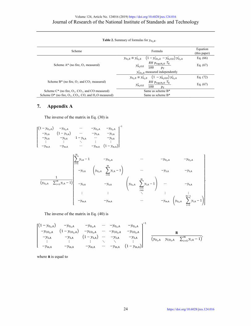
Table 2. Summary of formulas for 𝑦𝑦O2,E.
Scheme Formula Equation (this paper)
Scheme A* (no fire, O2 measured)
𝑦𝑦O2,E ≡ 𝑦𝑦O2,E∗ = �1 − 𝑦𝑦CO2,E
∗ − 𝑦𝑦H2O,E∗ � 𝑦𝑦O2,A
∗ Eq. (66)
𝑦𝑦H2O,E∗ =
𝑅𝑅𝑅𝑅100
𝑝𝑝vap,H2O(𝑇𝑇E)𝑝𝑝T
Eq. (67)
𝑦𝑦CO2,E∗ measured independently
Scheme B* (no fire, O2 and CO2 measured) 𝑦𝑦O2,E ≡ 𝑦𝑦O2,E
∗ = �1 − 𝑦𝑦H2O,E∗ � 𝑦𝑦O2,A
∗ Eq. (72)
𝑦𝑦H2O,E∗ =
𝑅𝑅𝑅𝑅100
𝑝𝑝vap,H2O(𝑇𝑇E)𝑝𝑝T
Eq. (67)
Scheme C* (no fire, O2, CO2, and CO measured) Same as scheme B* Scheme D* (no fire, O2, CO2, CO, and H2O measured) Same as scheme B*
7. Appendix A
The inverse of the matrix in Eq. (30) is
⎣⎢⎢⎢⎢⎡�1 − 𝑦𝑦O2,A� −𝑦𝑦O2,A ⋯ −𝑦𝑦O2,A −𝑦𝑦O2,A
−𝑦𝑦5,A �1 − 𝑦𝑦5,A� ⋯ −𝑦𝑦5,A −𝑦𝑦5,A−𝑦𝑦6,A −𝑦𝑦6,A (1 − 𝑦𝑦6,A) ⋯ −𝑦𝑦6,A⋮ ⋮ ⋱ ⋮ ⋮
−𝑦𝑦m,A −𝑦𝑦m,A ⋯ −𝑦𝑦m,A �1 − 𝑦𝑦m,A�⎦⎥⎥⎥⎥⎤−1
=1
�𝑦𝑦O2,A + � 𝑦𝑦𝑖𝑖,Am𝑖𝑖=5 − 1�
⎣⎢⎢⎢⎢⎢⎢⎢⎢⎢⎢⎢⎢⎡�𝑦𝑦𝑖𝑖,A
𝑚𝑚
𝑖𝑖=5
− 1 −𝑦𝑦O2,A ⋯ −𝑦𝑦O2,A −𝑦𝑦O2,A
−𝑦𝑦5,A �𝑦𝑦O2,A + �𝑦𝑦𝑖𝑖,A
m
𝑖𝑖=6
− 1� ⋯ −𝑦𝑦5,A −𝑦𝑦5,A
−𝑦𝑦6,A −𝑦𝑦6,A �𝑦𝑦O2,A +�𝑦𝑦𝑖𝑖,A
m
𝑖𝑖=5𝑖𝑖≠6
− 1� ⋯ −𝑦𝑦6,A
⋮ ⋮ ⋱ ⋮ ⋮
−𝑦𝑦m,A −𝑦𝑦m,A ⋯ −𝑦𝑦m,A �𝑦𝑦O2,A + �𝑦𝑦𝑖𝑖,A
m−1
𝑖𝑖=5
− 1�⎦⎥⎥⎥⎥⎥⎥⎥⎥⎥⎥⎥⎥⎤
.
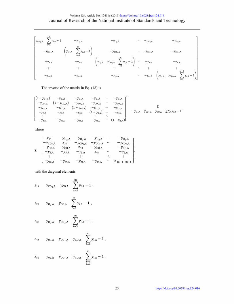
The inverse of the matrix in Eq. (40) is
⎣⎢⎢⎢⎢⎡�1 − 𝑦𝑦O2,A� −𝑦𝑦O2,A −𝑦𝑦O2,A ⋯ −𝑦𝑦O2,A −𝑦𝑦O2,A
−𝑦𝑦CO2,A �1 − 𝑦𝑦CO2,A� −𝑦𝑦CO2,A ⋯ −𝑦𝑦CO2,A −𝑦𝑦CO2,A
−𝑦𝑦5,A −𝑦𝑦5,A �1− 𝑦𝑦5,A� ⋯ −𝑦𝑦5,A −𝑦𝑦5,A⋮ ⋮ ⋮ ⋱ ⋱ ⋮
−𝑦𝑦m,A −𝑦𝑦m,A −𝑦𝑦m,A ⋯ −𝑦𝑦m,A �1− 𝑦𝑦m,A�⎦⎥⎥⎥⎥⎤−1
=𝐑𝐑
�𝑦𝑦O2,A + 𝑦𝑦CO2,A + � 𝑦𝑦𝑖𝑖,Am𝑖𝑖=5 − 1�
,
where 𝐑𝐑 is equal to
Volume 124, Article No. 124016 (2019) https://doi.org/10.6028/jres.124.016
Journal of Research of the National Institute of Standards and Technology
25 https://doi.org/10.6028/jres.124.016
⎣⎢⎢⎢⎢⎢⎢⎢⎢⎢⎢⎢⎡𝑦𝑦CO2,A + �𝑦𝑦𝑖𝑖,A
m
𝑖𝑖=5
− 1 −𝑦𝑦O2,A −𝑦𝑦O2,A ⋯ −𝑦𝑦O2,A −𝑦𝑦O2,A
−𝑦𝑦CO2,A �𝑦𝑦O2,A + �𝑦𝑦𝑖𝑖,A
m
𝑖𝑖=5
− 1� −𝑦𝑦CO2,A ⋯ −𝑦𝑦CO2,A −𝑦𝑦CO2,A
−𝑦𝑦5,A −𝑦𝑦5,A �𝑦𝑦O2,A + 𝑦𝑦CO2,A +�𝑦𝑦𝑖𝑖,A
m
𝑖𝑖=6
− 1� ⋯ −𝑦𝑦5,A −𝑦𝑦5,A
⋮ ⋮ ⋮ ⋱ ⋮ ⋮
−𝑦𝑦m,A −𝑦𝑦m,A −𝑦𝑦m,A ⋯ −𝑦𝑦m,A �𝑦𝑦O2,A + 𝑦𝑦CO2,A + � 𝑦𝑦𝑖𝑖,A
m−1
𝑖𝑖=5
− 1�⎦⎥⎥⎥⎥⎥⎥⎥⎥⎥⎥⎥⎤
.
The inverse of the matrix in Eq. (48) is
⎣⎢⎢⎢⎢⎢⎡�1 − 𝑦𝑦O2,A� −𝑦𝑦O2,A −𝑦𝑦O2,A −𝑦𝑦O2,A ⋯ −𝑦𝑦O2,A
−𝑦𝑦CO2,A �1 − 𝑦𝑦CO2,A� −𝑦𝑦CO2,A −𝑦𝑦CO2,A ⋯ −𝑦𝑦CO2,A
−𝑦𝑦CO,A −𝑦𝑦CO,A �1 − 𝑦𝑦CO,A� −𝑦𝑦CO,A ⋯ −𝑦𝑦CO,A
−𝑦𝑦5,A −𝑦𝑦5,A −𝑦𝑦5,A �1 − 𝑦𝑦5,A� ⋯ −𝑦𝑦5,A⋮ ⋮ ⋮ ⋮ ⋱ ⋮
−𝑦𝑦m,A −𝑦𝑦m,A −𝑦𝑦m,A −𝑦𝑦m,A ⋯ �1− 𝑦𝑦m,A�⎦⎥⎥⎥⎥⎥⎤−1
=𝐙𝐙
(𝑦𝑦O2,A + 𝑦𝑦CO2,A + 𝑦𝑦CO,A +∑ 𝑦𝑦𝑖𝑖,A − 1)m𝑖𝑖=5
,
where
𝐙𝐙 =
⎣⎢⎢⎢⎢⎡
𝑧𝑧11 −𝑦𝑦O2,A −𝑦𝑦O2,A −𝑦𝑦O2,A ⋯ −𝑦𝑦O2,A−𝑦𝑦CO2,A 𝑧𝑧22 −𝑦𝑦CO2,A −𝑦𝑦CO2,A ⋯ −𝑦𝑦CO2,A−𝑦𝑦CO,A −𝑦𝑦CO,A 𝑧𝑧33 −𝑦𝑦CO,A ⋯ −𝑦𝑦CO,A−𝑦𝑦5,A −𝑦𝑦5,A −𝑦𝑦5,A 𝑧𝑧44 ⋯ −𝑦𝑦5,A⋮ ⋮ ⋮ ⋮ ⋱ ⋮
−𝑦𝑦m,A −𝑦𝑦m,A −𝑦𝑦m,A −𝑦𝑦m,A ⋯ 𝑧𝑧(m−1)(m−1)⎦⎥⎥⎥⎥⎤
,
with the diagonal elements
𝑧𝑧11 = (𝑦𝑦CO2,A + 𝑦𝑦CO,A + �𝑦𝑦𝑖𝑖,A − 1),m
𝑖𝑖=5
𝑧𝑧22 = (𝑦𝑦O2,A + 𝑦𝑦CO,A + �𝑦𝑦𝑖𝑖,A − 1),m
𝑖𝑖=5
𝑧𝑧33 = (𝑦𝑦O2,A + 𝑦𝑦CO2,A + �𝑦𝑦𝑖𝑖 ,A − 1),m
𝑖𝑖=5
𝑧𝑧44 = (𝑦𝑦O2,A + 𝑦𝑦CO2,A + 𝑦𝑦CO,A + �𝑦𝑦𝑖𝑖,A − 1)m
𝑖𝑖=6
,
𝑧𝑧55 = (𝑦𝑦O2,A + 𝑦𝑦CO2,A + 𝑦𝑦CO,A + �𝑦𝑦𝑖𝑖,A − 1)m
𝑖𝑖=5𝑖𝑖≠6
,
Volume 124, Article No. 124016 (2019) https://doi.org/10.6028/jres.124.016
Journal of Research of the National Institute of Standards and Technology
26 https://doi.org/10.6028/jres.124.016
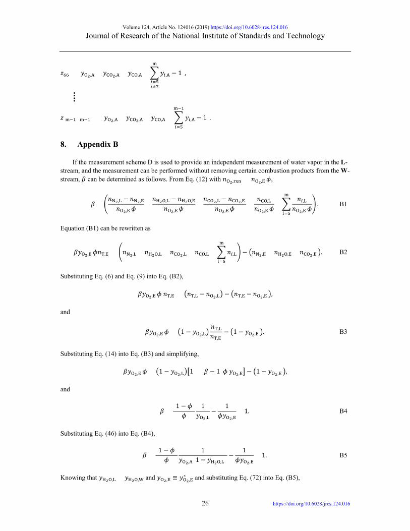
𝑧𝑧66 = (𝑦𝑦O2,A + 𝑦𝑦CO2,A + 𝑦𝑦CO,A + �𝑦𝑦𝑖𝑖,A − 1),m
𝑖𝑖=5𝑖𝑖≠7
⁞ 𝑧𝑧(m−1)(m−1) = (𝑦𝑦O2,A + 𝑦𝑦CO2,A + 𝑦𝑦CO,A + � 𝑦𝑦𝑖𝑖,A − 1).
m−1
𝑖𝑖=5
8. Appendix B
If the measurement scheme D is used to provide an independent measurement of water vapor in the L-
stream, and the measurement can be performed without removing certain combustion products from the W-stream, 𝛽𝛽 can be determined as follows. From Eq. (12) with 𝑛𝑛O2,rxn = 𝑛𝑛O2,E 𝜙𝜙,
𝛽𝛽 = �𝑛𝑛N2,L − 𝑛𝑛N2,E
𝑛𝑛O2,E 𝜙𝜙+𝑛𝑛H2O,L − 𝑛𝑛H2O,E
𝑛𝑛O2,E 𝜙𝜙+𝑛𝑛CO2,L − 𝑛𝑛CO2,E
𝑛𝑛O2,E 𝜙𝜙+
𝑛𝑛CO,L
𝑛𝑛O2,E 𝜙𝜙+ �
𝑛𝑛𝑖𝑖,L𝑛𝑛O2,E 𝜙𝜙
m
𝑖𝑖=5
� . (B1)
Equation (B1) can be rewritten as
𝛽𝛽𝑦𝑦O2,E 𝜙𝜙𝑛𝑛T,E = �𝑛𝑛N2,L + 𝑛𝑛H2O,L + 𝑛𝑛CO2,L + 𝑛𝑛CO,L + �𝑛𝑛𝑖𝑖,L
m
𝑖𝑖=5
� − �𝑛𝑛N2,E + 𝑛𝑛H2O,E + 𝑛𝑛CO2,E �. (B2)
Substituting Eq. (6) and Eq. (9) into Eq. (B2),
𝛽𝛽𝑦𝑦O2,E 𝜙𝜙 𝑛𝑛T,E = �𝑛𝑛T,L − 𝑛𝑛O2,L� − �𝑛𝑛T,E − 𝑛𝑛O2,E �,
and
𝛽𝛽𝑦𝑦O2,E 𝜙𝜙 = �1 − 𝑦𝑦O2,L�𝑛𝑛T,L
𝑛𝑛T,E − �1 − 𝑦𝑦O2,E �. (B3)
Substituting Eq. (14) into Eq. (B3) and simplifying,
𝛽𝛽𝑦𝑦O2,E 𝜙𝜙 = �1 − 𝑦𝑦O2,L��1 + (𝛽𝛽 − 1)𝜙𝜙 𝑦𝑦O2,E� − �1 − 𝑦𝑦O2,E �,
and
𝛽𝛽 =(1 − 𝜙𝜙)
𝜙𝜙1
𝑦𝑦O2,L−
1𝜙𝜙𝑦𝑦O2,E
+ 1. (B4)
Substituting Eq. (46) into Eq. (B4),
𝛽𝛽 =(1 − 𝜙𝜙)
𝜙𝜙1
𝑦𝑦O2,A(1 − 𝑦𝑦H2O,L)−
1𝜙𝜙𝑦𝑦O2,E
+ 1. (B5)
Knowing that 𝑦𝑦H2O,L = 𝑦𝑦H2O,W and 𝑦𝑦O2,E ≡ 𝑦𝑦O2,E
∗ and substituting Eq. (72) into Eq. (B5),
Volume 124, Article No. 124016 (2019) https://doi.org/10.6028/jres.124.016
Journal of Research of the National Institute of Standards and Technology
27 https://doi.org/10.6028/jres.124.016
𝛽𝛽 =(1 − 𝜙𝜙)
𝜙𝜙1
𝑦𝑦O2,A�1 − 𝑦𝑦H2O,W�−
1𝜙𝜙𝑦𝑦O2,A
∗ �1 − 𝑦𝑦H2O,E∗ �
+ 1. (B6)
From Eq. (73),
𝛽𝛽 =(1 − 𝜙𝜙)
𝜙𝜙1
𝑦𝑦O2,A�1 − 𝑦𝑦H2O,W�−
1𝜙𝜙𝑦𝑦O2,A
∗ �1 − 𝑦𝑦H2O,W∗ �
+ 1. (B7)
9. Appendix C
Based on the generalized framework developed here, the formulas for the four specific measurement
schemes (schemes A, B, C, and D) can be easily extended to a generalized measurement scheme that involves the dry-basis measurements of O2, CO2, CO, and S5 to S j major combustion product species with j < m. With � 𝑦𝑦𝑖𝑖 ,A
m𝑖𝑖=5 = � 𝑦𝑦𝑖𝑖,A
j𝑖𝑖=5 + � 𝑦𝑦𝑖𝑖 ,A
m𝑖𝑖=j+1 , one rewrites Eq. (49) as
⎣⎢⎢⎢⎢⎡𝑦𝑦O2,L𝑦𝑦CO2,L𝑦𝑦CO,L𝑦𝑦5,L⋮
𝑦𝑦m,L ⎦⎥⎥⎥⎥⎤
=𝑦𝑦N2,L
�1 − 𝑦𝑦O2,A − 𝑦𝑦CO2,A − 𝑦𝑦CO,A −� 𝑦𝑦𝑖𝑖,Aj𝑖𝑖=5 −� 𝑦𝑦𝑖𝑖 ,A
m𝑖𝑖=j+1 �
⎣⎢⎢⎢⎢⎡𝑦𝑦O2,A 𝑦𝑦CO2,A 𝑦𝑦CO,A𝑦𝑦5,A⋮
𝑦𝑦m,A ⎦⎥⎥⎥⎥⎤
. (C1)
If one assumes � 𝑦𝑦𝑖𝑖,A
m𝑖𝑖=j+1 ≪ 1, Eq. (C1) can be simplified to
⎣⎢⎢⎢⎢⎡𝑦𝑦O2,L𝑦𝑦CO2,L𝑦𝑦CO,L𝑦𝑦5,L⋮𝑦𝑦j,L ⎦
⎥⎥⎥⎥⎤
=𝑦𝑦N2,L
�1 − 𝑦𝑦O2,A − 𝑦𝑦CO2,A − 𝑦𝑦CO,A −� 𝑦𝑦𝑖𝑖 ,Aj𝑖𝑖=5 �
⎣⎢⎢⎢⎢⎡𝑦𝑦O2,A 𝑦𝑦CO2,A 𝑦𝑦CO,A𝑦𝑦5,A⋮𝑦𝑦j,A ⎦
⎥⎥⎥⎥⎤
. (C2)
Substituting Eq. (C2) and Eq.(52) into Eq. (3),
𝜙𝜙 = 1 −𝑛𝑛T,L 𝑦𝑦O2,L
𝑛𝑛T,E 𝑦𝑦O2,E= 1 −
𝑦𝑦N2,E
𝑦𝑦O2,E
𝑦𝑦O2,A
�1 − 𝑦𝑦O2,A − 𝑦𝑦CO2,A − 𝑦𝑦CO,A −� 𝑦𝑦𝑖𝑖,Aj𝑖𝑖=5 �
. (C3)
Substituting Eq. (71) into Eq. (C3), simplifying, and noting that 𝑦𝑦O2,E
∗ ≡ 𝑦𝑦O2,E and 𝑦𝑦N2,E∗ ≡ 𝑦𝑦N2,E,
𝜙𝜙 =𝑦𝑦O2,A∗ �1 − 𝑦𝑦CO2,A − 𝑦𝑦CO,A −� 𝑦𝑦𝑖𝑖 ,A
j𝑖𝑖=5 � − 𝑦𝑦O2,A�1 − 𝑦𝑦CO2,A
∗ �
𝑦𝑦O2,A∗ �1 − 𝑦𝑦O2,A − 𝑦𝑦CO2,A − 𝑦𝑦CO,A −� 𝑦𝑦𝑖𝑖,A
j𝑖𝑖=5 �
. (C4)
Volume 124, Article No. 124016 (2019) https://doi.org/10.6028/jres.124.016
Journal of Research of the National Institute of Standards and Technology
28 https://doi.org/10.6028/jres.124.016
10. References
[1] Babrauskas V, Peacock, RD (1992) Heat release rate: The single most important variable in fire hazard. Fire Safety Journal 18:255–272. https://doi.org/10.1016/0379-7112(92)90019-9
[2] Thornton WM (1917) The relation of oxygen to the heat of combustion of organic compounds. Philosophical Magazine 33:196–203. https://doi.org/10.1080/14786440208635627
[3] Babrauskas V (1984) Development of the cone calorimeter―A bench-scale heat release rate apparatus based on oxygen consumption. Fire and Materials 8(2):81–95. https://doi.org/10.1002/fam.810080206
[4] Bryant RA, Ohlemiller TJ, Johnsson EK, Hamins A, Grove BS, Guthrie WF, Maranghides A, Mulholland GW (2004) The NIST 3 Megawatt Quantitative Heat Release Rate Facility—Description and Procedures. (National Institute of Standards and Technology, Gaithersburg, MD), NIST Interagency/Internal Report (NISTIR) 7052. http://doi.org/10.6028/NIST.IR.7052
[5] Huggett C (1980) Estimation of rate of heat release by means of oxygen consumption measurements. Fire and Materials 4(2):61–65. https://doi.org/10.1002/fam.810040202
[6] Parker WJ (1982) Calculations of the Heat Release Rate by Oxygen Consumption for Various Applications. (U.S. Department of Commerce, Washington D.C.), National Bureau of Standards Interagency/Internal Report (NBSIR) 81-2427-1. http://doi.org/10.6028/NBS.IR.81-2427-1
[7] Parker WJ (1984) Calculations of the heat release rate by oxygen consumption for various applications. Journal of Fire Sciences 2(5):380–395. https://doi.org/10.1177/073490418400200505
[8] Janssens ML (1991) Measuring rate of heat release by oxygen consumption. Fire Technology 27(3):234–249. https://doi.org/10.1007/BF01038449
[9] Janssens ML, Parker WJ (1992) Oxygen consumption calorimetry. Heat Release in Fires, eds Babrauskas V, Grayson SJ (Elsevier, New York), Chapter 3, pp 31–59.
[10] Brohez S, Delvosalle C, Marlair G, Tewarson A (2000) The measurement of heat release from oxygen consumption in sooty fires. Journal of Fire Sciences 18(5):327–353. https://doi.org/10.1177/073490410001800501
[11] Chow WK, Han SS (2011) Heat release rate calculation in oxygen consumption calorimetry. Applied Thermal Engineering 31:304–310. https://doi.org/10.1016/j.applthermaleng.2010.09.010
[12] Lattimer BY, Beitel JJ (1998) Evaluation of heat release rate equations used in standard test methods. Fire and Materials 22(4):167–173. https://doi.org/10.1002/(SICI)1099-1018(1998070)22:4%3C167::AID-FAM649%3E3.0.CO;2-M
[13] Amundson NR (1966) Mathematical Methods in Chemical Engineering: Matrices and Their Application (Prentice-Hall, Englewood Cliffs, NJ).
[14] Himmelblau DM (1982) Basic Principles and Calculations in Chemical Engineering (Prentice-Hall, Englewood Cliffs, NJ), 4th Ed.
[15] Levenspiel O (1972) Chemical Reaction Engineering (John Wiley & Sons, New York), 2nd Ed. [16] Kreyszig E (1983) Advanced Engineering Mathematics (John Wiley & Sons, New York), 5th Ed.
About the author: Jiann C. Yang is the deputy division chief in the Fire Research Division at NIST. The National Institute of Standards and Technology is an agency of the U.S. Department of Commerce.


![OUTER DERIVATIONS OF LIE ALGEBRAS · 1967] OUTER DERIVATIONS OF LIE ALGEBRAS 267 outer derivations is a linear sum of the outer derivations, which are obtained as in the first part](https://img.pdfslide.us/doc/110x75/5ec52027613ab73b287ddf89/outer-derivations-of-lie-algebras-1967-outer-derivations-of-lie-algebras-267-outer.jpg)