Article

Designing Wood Supply Scenarios from ForestInventories with Stratified Predictions

Philipp Kilham 1,2,* ID , Gerald Kändler 1, Christoph Hartebrodt 1, Anne-Sophie Stelzer 1 ID

and Ulrich Schraml 1

1 Forest Research Institute Baden-Württemberg (FVA), 79110 Freiburg, Germany;gerald.kaendler@forst.bwl.de (G.K.); christoph.hartebrodt@forst.bwl.de (C.H.);anne-sophie.stelzer@forst.bwl.de (A.-S.S.); ulrich.schraml@forst.bwl.de (U.S.)

2 Faculty of Environment and Natural Resources, University of Freiburg, 79110 Freiburg, Germany* Correspondence: philipp.kilham@forst.bwl.de or philipp-kilham@posteo.de; Tel.: +49-761-401-8312

Received: 11 January 2018; Accepted: 2 February 2018; Published: 6 February 2018

Abstract: Forest growth and wood supply projections are increasingly used to estimate the futureavailability of woody biomass and the correlated effects on forests and climate. This researchparameterizes an inventory-based business-as-usual wood supply scenario, with a focus on southwestGermany and the period 2002–2012 with a stratified prediction. First, the Classification and RegressionTrees algorithm groups the inventory plots into strata with corresponding harvest probabilities.Second, Random Forest algorithms generate individual harvest probabilities for the plots of eachstratum. Third, the plots with the highest individual probabilities are selected as harvested until theharvest probability of the stratum is fulfilled. Fourth, the harvested volume of these plots is predictedwith a linear regression model trained on harvested plots only. To illustrate the pros and cons ofthis method, it is compared to a direct harvested volume prediction with linear regression, and acombination of logistic regression and linear regression. Direct harvested volume regression predictscomparable volume figures, but generates these volumes in a way that differs from business-as-usual.The logistic model achieves higher overall classification accuracies, but results in underestimations oroverestimations of harvest shares for several subsets of the data. The stratified prediction methodbalances this shortcoming, and can be of general use for forest growth and timber supply projectionsfrom large-scale forest inventories.

Keywords: aggregated wood supply; national forest inventory; business-as-usual; stratifiedprediction; Classification and Regression Trees (CART); Random Forest (RF)

1. Introduction

Emerging bioeconomy strategies consider lignocelluloses from forests as an alternative to fossilraw materials [1–3], suggesting that the demand for woody biomass is likely to increase globally [4,5].At the same time, forest reference level scenarios gain increasing importance with regards to the UnitedNations Framework Convention on Climate Change (UNFCCC) [6,7]. National forest inventories (NFIs)and aggregated forest growth and wood supply modeling (AFGWSM) can be used to estimate thefuture availability of woody biomass and the correlated effects on forests and climate. NFIs have beenestablished in several countries to generate data about forest conditions, dynamics, and productivity.Today, most European and North American countries conduct forest inventories based on statisticalsampling [8–10]. In addition, many countries use or are developing AFGWSMs that are directlyconnected to the respective NFI data [11].

Although wood supply scenarios are not explicitly forecasts, they are expected to generateresults that qualify as decision support for policymakers, administrations, industry, and other interestgroups [12]. As such, they are supposed to be “a coherent, internally consistent and plausible

Forests 2018, 9, 77; doi:10.3390/f9020077 www.mdpi.com/journal/forests

Forests 2018, 9, 77 2 of 24

description of a possible state of the world” [13] (p. 799) [14]. Among possible themes for woodsupply scenarios, business-as-usual (BAU) scenarios are of specific importance. While focusing ratheron short-term trends, these scenario types can establish a baseline according to which other scenarioscan be shaped or referenced [15].

To design BAU scenarios for AFGWSMs, “heterogeneous forest land and owners withheterogeneous objectives” [16] (pp. 200–201) have to be integrated. Concept-driven studies thatapply theoretical preconceptions to the data [17–20] can be differentiated from data-driven methodsthat—as is the goal of this research—aim to learn these concepts from the data first [21].

In the past, numerous data-driven studies have focused on the objectives and harvest decisionsof forest owners. An overview of research on the non-industrial private forest (NIPF) sector, whichwas the subject of the majority of these studies, is provided by Amacher et al. [22] and Beach et al. [23].A common method is to use panels or surveys that are analyzed with various specifications of tobit orlogit models [24–28]. Only a few panel-based studies have had access to large datasets [29,30], and theattitude towards or intention to harvest is often measured rather than the actual harvest [31].

NFI-based studies offer the advantage that forest development and timber harvests can be derivedfrom a large number of inventory plots that are often permanent and repeatedly measured [8,32].Unlike survey-based studies, a representative fraction of the actual resource is considered as theprincipal research unit (PRU), as opposed to the individual forest owner or manager. Several studiesused NFI data to review AFGWSM scenarios [33–35]. Another group of studies used NFI or otherforest inventory data to investigate and/or project harvest behavior using regression models or othermachine learning algorithms [21,36–39].

However, when BAU scenarios are learned and projected from NFI data, researchers areconfronted with two major issues. First, unlike survey research, NFI-based studies often lackspecific and relatable information about the relevant decisionmakers (forest owners or managers).For example, a study with access to linked inventory and survey data reported impacts of the morespecific ownership characteristics of education and income on harvest probabilities [36]. However,this information is often not available. In the case of the German NFI, for example, opportunities tocollect information on individual plot owners are limited, since the exact location and land ownershipof NFI tracts cannot be revealed. Second, on the PRU level, NFIs often produce noisy data that is notrepresentative of the forest area upon which a harvest decision is made. Instead, data only becomerepresentative at higher aggregation levels.

The principal aim of this research was to parameterize a BAU wood supply scenario from NFIdata by dealing explicitly with this restriction. The quality of the scenario was judged on its abilityto reproduce 2002–2012 timber harvests reported by the NFI. To consider a BAU scenario as wellcalibrated, not only overall NFI harvested volumes should be well captured. The scenario shouldalso retrace NFI harvested volumes throughout characteristics of the inventory data (e.g., stand typesand timber dimensions). Furthermore, it was considered important that the observed occurrence ornon-occurrence of harvest interventions at plot level be reflected in the scenario.

To address this issue, a stratified machine learning approach based on the Classification andRegression Tree (CART) algorithm [40] was designed and tested in the scope of this research.The method optimizes the prediction of harvest occurrences and harvest shares towards patterns ofthe original inventory. It can be used as an upstream model that predicts harvest decisions (yes orno) for individual inventory plots. Commonly, overall cut-off benchmarks [41] are used to convertpredicted probabilities into a binary decision. In contrast, the presented method uses the learnedharvest probabilities of strata as decision criteria. The first rule is that this probability must be metby the number of plots selected as harvested in each stratum. For the selection of individual plotsto be harvested per stratum, two alternative options are presented: random selection (assuming thatno other attributes would influence the harvest decisions in the strata), or a Random Forest (RF)algorithm [42] trained on the training data of the corresponding stratum. Once the plots are predicted

Forests 2018, 9, 77 3 of 24

as harvested by the stratified approach, linear regression trained on harvested inventory plots onlycan be used to predict the harvested volumes for these plots.

To assess the pros and cons of the presented stratified harvest prediction approach, results arecompared to a direct harvested volume prediction with linear regression, as well as to a two-stepapproach with logistic regression (using an overall cut-off benchmark), followed by linear regressiontrained on harvested inventory plots only.

A unique feature of this paper is that existing machine learning techniques are adapted andcombined to serve specific requirements of large-scale inventory based harvest decisions and harvestedvolume predictions. The results of this research can be used to project business-as-usual timber suppliesdirectly for a 10-year period (in this case 2012–2022). Furthermore, the results can inform harvestscenarios, which are used in combination with NFI-based forest growth projections, as described byKändler and Riemer [43].

2. Materials and Method

2.1. Focus

The regional focus of the study was Baden-Württemberg, a German federal state located insouthwest Germany. Baden-Württemberg shares borders with Switzerland (south) and France (west).The state covers an area of around 35,750 km2. Around 38.4% of this area is considered to be forest.Around 40% of the forest area is managed by communities, 35.9% is managed by private owners,23.6% is managed by the state, and only 0.5% is managed by federal bodies [44]. A small proportion(around 1.5%) of the forest that was classified as community property was parish or cooperative forestin 2002. Spruce (Picea abies (L.) Karst.) is the most common tree species, and beech (Fagus sylvatica L.)is the most common broadleaved tree species in the region. The analysis focused on a 10-year periodfrom 2002 to 2012. This corresponds to the period between the second and third German NFIs. In thisperiod, forests in Baden-Württemberg were affected by the aftermath of storm Lothar (1999), a droughtperiod in 2003, and storm Kyrill (2007).

With reference to the year 2008, 690 saw mills (116 with more than 10 employees), 52 woodcomposite producers, and 128 pulp and paper producers were counted within Baden-Württemberg.In 2008, a higher number of saw mills was registered in the west—especially in the southwest—ofthe federal state. However, the saw mills in the east—especially in the northeast—recorded muchhigher turnovers per holding. The timber market was dominated by spruce and fir (Abies alba Mill.),which accounted for around 80% of the timber sold via the federal state’s forest service in the period2000–2009. With reference to the same period, 88% of the timber sold via the forest service was stemwood [45].

2.2. Data Sources

NFI data (available online at Thünen Institut [44]) constituted the principal data source for thisresearch. To date, three NFIs have been conducted in Germany; the first from 1986 to 1988, the secondfrom 2001 to 2002 and the third from 2011 to 2012. The German NFI has been designed as a systematicsingle-level cluster sampling, with tracts (clusters of one to four plots) as primary sampling units [46].Plots are permanently marked and remeasured within the scope of each inventory. For this research,trees registered via the angle-count method (caliper threshold 7 cm) were of the highest relevance.For Baden-Württemberg, data from 8963 tracts, with a total of 35,743 plots, were collected on a2 km × 2 km grid in the scope of the second NFI. Out of these, 13,619 plots were located withinforest areas [46,47]. In the scope of this research, only the plots that were registered as accessible,productive forest not owned by the federal government (see Section 2.4) were used. The final set ofNFI plots included 11,722 plots from 4306 tracts, and did not contain missing values for any of theincluded variables.

Forests 2018, 9, 77 4 of 24

2.3. Response Attributes

Both response and predicting attributes were registered in the scope of the NFI, or calculatedfrom NFI data (see Tables A1 and A2). The variable harvested volumes was expressed as cubic meterstanding volume over bark (m3ob) per ha within a 10-year period (2002–2012). Since the exact yearof harvest remains unknown, harvested volumes correspond to tree dimensions estimated with theSloboda trend function for the mid-period (2007) [46,48]. To calculate harvested volumes, only treesregistered via angle count sampling were used. Moreover, only trees indicated as selectively cut orharvested by clear felling and removed from the forest within the period of interest were considered.To extrapolate data from the angle-count method to one-hectare values, tree representation factorsfrom the beginning of the period (second NFI) were used [46].

The variable harvest decision was generated on plot level as a binominal representation ofharvested volumes with the characteristics yes (harvested volumes > 0) and no (harvested volumes = 0).

2.4. Predicting Attributes

The selection of potential influencing factors (predicting attributes) was determined using twocriteria: First, existing concepts (derived from the literature) of how forest owners or managers makeharvest decisions, and, second, the availability of information that could be linked directly to NFI plots.Based on this, the following 11 attributes were included in this research: Stand-related attributes (standtype, standing volume, average plot diameter at breast height (DBH), and average plot age), site-relatedattributes (site index, harvest condition, slope, and altitude above sea level (a.s.l.), ownership-relatedattributes (ownership type), and policy-related attributes (nature park, and nature protected area).

The variable stand type differentiated between spruce, fir, and Douglas fir (Pseudotsuga menziesii(Mirb.) Franco) stands (conifers 1); pine (Pinus sylvestris L.), larch (Larix decidua Mill.), and othersoftwood stands (conifers 2); deciduous stands (deciduous); mixed stands with spruce, fir or Douglasfir as principal species (mixed 1); and other mixed stands (mixed 2). A description of the stand typescan be found in Table A3. The variable standing volume referred to the standing volume across all ofthe species at the time of the second NFI. It was indicated as m3ob per ha. The variable average plotDBH was calculated as the average DBH of all of the trees (across all species), which was measuredon a plot by taking the representation factors of the sample trees into account. Only sample trees ofthe dominant and predominant forest stories were considered. The variable average plot age wascalculated in a similar way to the average DBH, but with regards to the age of the individual trees andfor the mid-term of the period (2007).

The variable site index [21] was expressed as the yearly average total increment in m3ob per haat the age of 100 years, and originated from Ministerium für Ländlichen Raum (MLR) [49]. Slope,distance to the road, and terrain roughness are identified in the literature as having an impact on woodproduction through harvesting costs and profitability [21,38,50]. The variable harvest condition wasregistered in the scope of the third NFI. It included the classes favorable and unfavorable. Unfavorableharvest conditions refer to slopes greater than 30% that were not suitable for harvesters due to chunksof rocks, pits, or spring horizons. No differentiation was made between the necessity and non-necessityof cableways, as both groups contained only low numbers of NFI plots. The class also containedplots with large machine track distances (>150 m), and large distances between forest plot and nearestdriveway (>1 km) [47]. The attribute slope provided information about the slope at the location of theindividual NFI plot in percent, and was also tested separately from harvest condition. The variablealtitude (m a.s.l.) was included, since previous research established a relationship between altitudinalranges (elevation) and timber harvests. Sterba et al. [33] found that the scenario they analyzedunderestimated salvage harvests of smaller DBH classes at lower elevations. They attribute thisfinding to a higher susceptibility of these forest types to bark beetles, which they trace back to thebiology of Ips typographus and Ips chalcographus. Thürig and Schelhaas [35] pointed towards factorsrelated to altitude (a.s.l.) such as harvesting costs, accessibility, and forest functions (e.g., protectionfrom avalanches in higher altitudes).

Forests 2018, 9, 77 5 of 24

Different ownership types are considered to show different harvesting behaviors [17,18,37].The analyzed attribute ownership type included the subgroups federal, state, community, and privateforest. The private forest was further differentiated into large (>500 ha), medium (5–500 ha), and small(<5 ha). These size classes referred to the total forest area owned by the proprietor of the respectiveNFI plots within Germany. Federal plots were excluded from the analysis, since the NFI recorded onlya few plots of this ownership type.

The variables nature park and nature protection area indicate whether the area surrounding anNFI plot was covered by the respective directive.

Some attributes could not be included in the analysis. Profitability is a factor that is oftenconsidered with reference to harvest decisions [37]. However, the calculation of potential returnsat plot level would require pre-assumptions about applied harvest regimes, and a pre-selection ofindividual trees to be harvested. This would then contradict the data-driven approach followed inthis research. The concept of profitability could, therefore, only be tested from a cost perspective byincluding the attributes harvest condition and slope. Several studies divide medium and small-scaleforest owners into various subcategories [25,51]. Due to a lack of information and small sample sizes,these subcategories could not be analyzed.

For the ordinary least squares (OLS) regressions and the logistic regression (LREG), numericvariables were centered.

2.5. Research Design

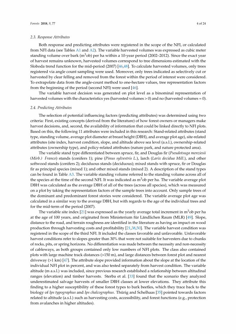
Figure 1 shows the research design for learning and predicting harvest decisions and harvestedvolumes. This paper focuses predominantly on the stratified methods used to learn and predict thebinary harvest decision. The location of these elements within the prediction chain is emphasized inFigure 1 (bold and dashed lines).

Forests 2018, 9, x FOR PEER REVIEW 5 of 24

Different ownership types are considered to show different harvesting behaviors [17,18,37]. The analyzed attribute ownership type included the subgroups federal, state, community, and private forest. The private forest was further differentiated into large (>500 ha), medium (5–500 ha), and small (<5 ha). These size classes referred to the total forest area owned by the proprietor of the respective NFI plots within Germany. Federal plots were excluded from the analysis, since the NFI recorded only a few plots of this ownership type.

The variables nature park and nature protection area indicate whether the area surrounding an NFI plot was covered by the respective directive.

Some attributes could not be included in the analysis. Profitability is a factor that is often considered with reference to harvest decisions [37]. However, the calculation of potential returns at plot level would require pre-assumptions about applied harvest regimes, and a pre-selection of individual trees to be harvested. This would then contradict the data-driven approach followed in this research. The concept of profitability could, therefore, only be tested from a cost perspective by including the attributes harvest condition and slope. Several studies divide medium and small-scale forest owners into various subcategories [25,51]. Due to a lack of information and small sample sizes, these subcategories could not be analyzed.

For the ordinary least squares (OLS) regressions and the logistic regression (LREG), numeric variables were centered.

2.5. Research Design

Figure 1 shows the research design for learning and predicting harvest decisions and harvested volumes. This paper focuses predominantly on the stratified methods used to learn and predict the binary harvest decision. The location of these elements within the prediction chain is emphasized in Figure 1 (bold and dashed lines).

The createDataPartition function of the caret R package [52,53] was used to split the data into training and test sets. This method was chosen since setting aside a test set completely is preferable to cross-validation or boosting if enough data is available [54]. Models were trained and refined on training data only (75% of the data). The fitted models were then applied to the test data one time to predict harvest decision and harvested volumes. Finally, the test set outcome of the various models was compared to NFI results.

Figure 1. Research design. 1 Direct refers to a one-step training and prediction method where harvested volumes are predicted directly. Downstream and upstream models are the components of Figure 1. Research design. 1 Direct refers to a one-step training and prediction method where harvestedvolumes are predicted directly. Downstream and upstream models are the components of a two-stepapproach, where the harvest decision is predicted first (upstream), and subsequently (downstream),harvested volumes are predicted for plots predicted as harvested.

Forests 2018, 9, 77 6 of 24

The createDataPartition function of the caret R package [52,53] was used to split the data intotraining and test sets. This method was chosen since setting aside a test set completely is preferableto cross-validation or boosting if enough data is available [54]. Models were trained and refined ontraining data only (75% of the data). The fitted models were then applied to the test data one time topredict harvest decision and harvested volumes. Finally, the test set outcome of the various modelswas compared to NFI results.

2.6. Stratified Learning and Prediction

2.6.1. Stratification Model

The Classification and Regression Trees (CART) algorithm [40] built the foundation of the stratifiedprediction method. They were used to stratify the data, and generated harvest probabilities foreach stratum.

CART is a tree-based model that partitions the feature space into rectangles, and subsequentlyfits a simple model in each rectangle. The method stratifies the data into strata with high and lowprobabilities [54]. CART uses the Gini index, and applies the split that maximizes the Gini [55].

A drawback of CART is that only one variable at a time can be considered [56], and that singletrees are considered unstable [57]. A commonly used method for overcoming these issues is to grow anumber of trees as implemented in Random Forest (RF) models [42]. However, this procedure resultsin individual harvest probabilities per plot (share of trees that voted for yes), and is not suited to astratified approach.

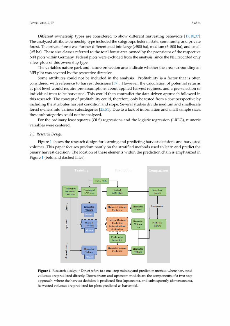
To generate the classification tree (method = class), the rpart function of R’s rpart package [58]was used. The model was trained on the complete training set, including the entire set of predictingattributes. The minimum number of observations per terminal leaf was set at 100 to secure sufficientdata in both the training and test sets. As a consequence, a node needed to include a minimum of200 observations before a split was attempted [59]. To reduce overfitting, the original tree was prunedto a size that minimized the cross-validation error calculated by a 10-fold cross-validation within thetraining set [60]. Using this method, the trained classification tree was pruned to 18 leaves. The finaloutcome is shown in Figure 2.

Within the prediction process, the trained CART tree was applied to the test set. The test setplots were thereby assigned to the various leaves of the tree. Thus, each leaf (stratum) had a harvestprobability (learned from the training set), and contained a number of test set plots.

Forests 2018, 9, 77 7 of 24Forests 2018, 9, x FOR PEER REVIEW 7 of 24

Figure 2. Pruned outcome of the Classification and Regression Tree (CART) algorithm showing harvest probabilities (P) and number of training set plots (N) for the 18 leaves of the tree (leaf numbers sorted by harvest probability). The branch size is related to the number of training set plots sent towards the respective direction (DBH: average stand diameter at breast height).

2.6.2. Stratified Random Prediction

One option to predict harvest decisions for test set plots within the strata was to assume that no additional criteria would influence the actual harvest decision within a stratum.

Thus, within each stratum, a number of test set plots was randomly selected as harvested in accordance with the specific harvest probability of the stratum. For example, from a stratum that contained 100 test set plots and a harvest probability of 0.6, 60 plots were randomly selected as harvested.

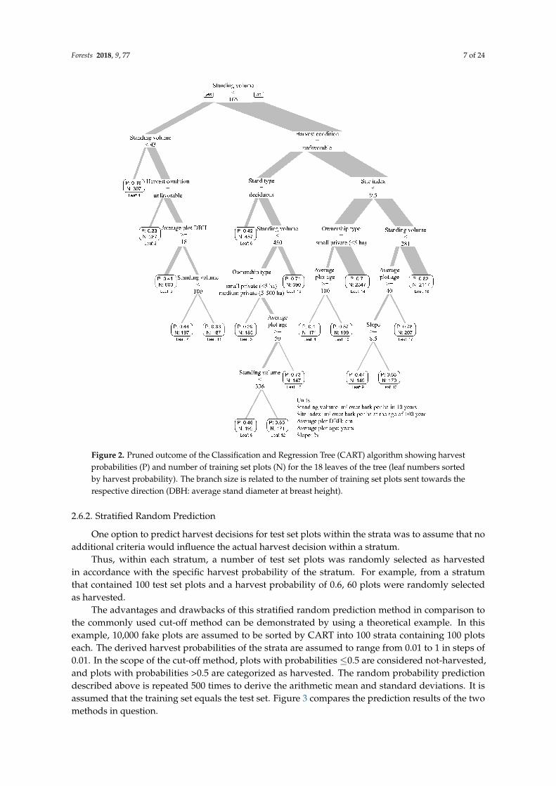
The advantages and drawbacks of this stratified random prediction method in comparison to the commonly used cut-off method can be demonstrated by using a theoretical example. In this example, 10,000 fake plots are assumed to be sorted by CART into 100 strata containing 100 plots each. The derived harvest probabilities of the strata are assumed to range from 0.01 to 1 in steps of 0.01. In the scope of the cut-off method, plots with probabilities ≤0.5 are considered not-harvested, and plots with probabilities >0.5 are categorized as harvested. The random probability prediction described above is repeated 500 times to derive the arithmetic mean and standard deviations. It is assumed that the training set equals the test set. Figure 3 compares the prediction results of the two methods in question.

Figure 2. Pruned outcome of the Classification and Regression Tree (CART) algorithm showing harvestprobabilities (P) and number of training set plots (N) for the 18 leaves of the tree (leaf numbers sortedby harvest probability). The branch size is related to the number of training set plots sent towards therespective direction (DBH: average stand diameter at breast height).

2.6.2. Stratified Random Prediction

One option to predict harvest decisions for test set plots within the strata was to assume that noadditional criteria would influence the actual harvest decision within a stratum.

Thus, within each stratum, a number of test set plots was randomly selected as harvestedin accordance with the specific harvest probability of the stratum. For example, from a stratumthat contained 100 test set plots and a harvest probability of 0.6, 60 plots were randomly selectedas harvested.

The advantages and drawbacks of this stratified random prediction method in comparison tothe commonly used cut-off method can be demonstrated by using a theoretical example. In thisexample, 10,000 fake plots are assumed to be sorted by CART into 100 strata containing 100 plotseach. The derived harvest probabilities of the strata are assumed to range from 0.01 to 1 in steps of0.01. In the scope of the cut-off method, plots with probabilities ≤0.5 are considered not-harvested,and plots with probabilities >0.5 are categorized as harvested. The random probability predictiondescribed above is repeated 500 times to derive the arithmetic mean and standard deviations. It isassumed that the training set equals the test set. Figure 3 compares the prediction results of the twomethods in question.

Forests 2018, 9, 77 8 of 24

Forests 2018, 9, x FOR PEER REVIEW 8 of 24

(a) (b) (c)

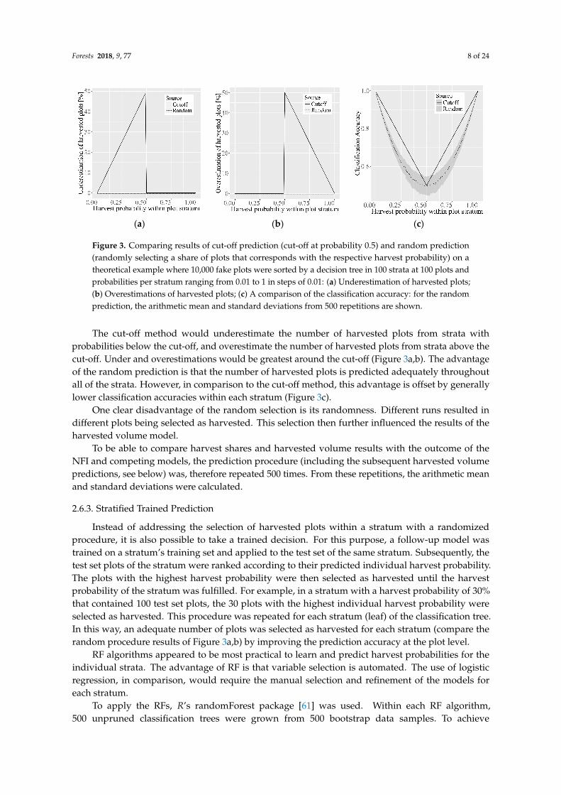
Figure 3. Comparing results of cut-off prediction (cut-off at probability 0.5) and random prediction (randomly selecting a share of plots that corresponds with the respective harvest probability) on a theoretical example where 10,000 fake plots were sorted by a decision tree in 100 strata at 100 plots and probabilities per stratum ranging from 0.01 to 1 in steps of 0.01: (a) Underestimation of harvested plots; (b) Overestimations of harvested plots; (c) A comparison of the classification accuracy: for the random prediction, the arithmetic mean and standard deviations from 500 repetitions are shown.

The cut-off method would underestimate the number of harvested plots from strata with probabilities below the cut-off, and overestimate the number of harvested plots from strata above the cut-off. Under and overestimations would be greatest around the cut-off (Figure 3a,b). The advantage of the random prediction is that the number of harvested plots is predicted adequately throughout all of the strata. However, in comparison to the cut-off method, this advantage is offset by generally lower classification accuracies within each stratum (Figure 3c).

One clear disadvantage of the random selection is its randomness. Different runs resulted in different plots being selected as harvested. This selection then further influenced the results of the harvested volume model.

To be able to compare harvest shares and harvested volume results with the outcome of the NFI and competing models, the prediction procedure (including the subsequent harvested volume predictions, see below) was, therefore repeated 500 times. From these repetitions, the arithmetic mean and standard deviations were calculated.

2.6.3. Stratified Trained Prediction

Instead of addressing the selection of harvested plots within a stratum with a randomized procedure, it is also possible to take a trained decision. For this purpose, a follow-up model was trained on a stratum’s training set and applied to the test set of the same stratum. Subsequently, the test set plots of the stratum were ranked according to their predicted individual harvest probability. The plots with the highest harvest probability were then selected as harvested until the harvest probability of the stratum was fulfilled. For example, in a stratum with a harvest probability of 30% that contained 100 test set plots, the 30 plots with the highest individual harvest probability were selected as harvested. This procedure was repeated for each stratum (leaf) of the classification tree. In this way, an adequate number of plots was selected as harvested for each stratum (compare the random procedure results of Figure 3a,b) by improving the prediction accuracy at the plot level.

RF algorithms appeared to be most practical to learn and predict harvest probabilities for the individual strata. The advantage of RF is that variable selection is automated. The use of logistic regression, in comparison, would require the manual selection and refinement of the models for each stratum.

To apply the RFs, R’s randomForest package [61] was used. Within each RF algorithm, 500 unpruned classification trees were grown from 500 bootstrap data samples. To achieve modifications between the trees, not all, but variables were sampled and considered in order to decide on the best split (where is the total number of considered variables, in this research: =

Figure 3. Comparing results of cut-off prediction (cut-off at probability 0.5) and random prediction(randomly selecting a share of plots that corresponds with the respective harvest probability) on atheoretical example where 10,000 fake plots were sorted by a decision tree in 100 strata at 100 plots andprobabilities per stratum ranging from 0.01 to 1 in steps of 0.01: (a) Underestimation of harvested plots;(b) Overestimations of harvested plots; (c) A comparison of the classification accuracy: for the randomprediction, the arithmetic mean and standard deviations from 500 repetitions are shown.

The cut-off method would underestimate the number of harvested plots from strata withprobabilities below the cut-off, and overestimate the number of harvested plots from strata above thecut-off. Under and overestimations would be greatest around the cut-off (Figure 3a,b). The advantageof the random prediction is that the number of harvested plots is predicted adequately throughoutall of the strata. However, in comparison to the cut-off method, this advantage is offset by generallylower classification accuracies within each stratum (Figure 3c).

One clear disadvantage of the random selection is its randomness. Different runs resulted indifferent plots being selected as harvested. This selection then further influenced the results of theharvested volume model.

To be able to compare harvest shares and harvested volume results with the outcome of theNFI and competing models, the prediction procedure (including the subsequent harvested volumepredictions, see below) was, therefore repeated 500 times. From these repetitions, the arithmetic meanand standard deviations were calculated.

2.6.3. Stratified Trained Prediction

Instead of addressing the selection of harvested plots within a stratum with a randomizedprocedure, it is also possible to take a trained decision. For this purpose, a follow-up model wastrained on a stratum’s training set and applied to the test set of the same stratum. Subsequently, thetest set plots of the stratum were ranked according to their predicted individual harvest probability.The plots with the highest harvest probability were then selected as harvested until the harvestprobability of the stratum was fulfilled. For example, in a stratum with a harvest probability of 30%that contained 100 test set plots, the 30 plots with the highest individual harvest probability wereselected as harvested. This procedure was repeated for each stratum (leaf) of the classification tree.In this way, an adequate number of plots was selected as harvested for each stratum (compare therandom procedure results of Figure 3a,b) by improving the prediction accuracy at the plot level.

RF algorithms appeared to be most practical to learn and predict harvest probabilities for theindividual strata. The advantage of RF is that variable selection is automated. The use of logisticregression, in comparison, would require the manual selection and refinement of the models foreach stratum.

To apply the RFs, R’s randomForest package [61] was used. Within each RF algorithm,500 unpruned classification trees were grown from 500 bootstrap data samples. To achieve

Forests 2018, 9, 77 9 of 24

modifications between the trees, not all, but√

p variables were sampled and considered in orderto decide on the best split (where p is the total number of considered variables, in this research:p =√

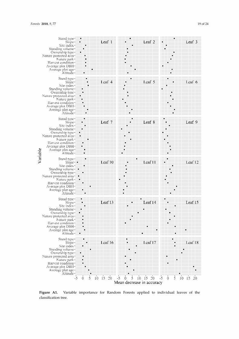
11 ∼= 3). Harvest probabilities for the individual test set plots were then predicted by calculatingthe share of the 500 trees that voted for harvest = yes [42,61,62]. For each RF variable, importancewas read out as the mean decrease in accuracy (see Figure A1) with the varImpPlot function ofthe randomForest package [61]. The 11 predicting variables were included within all of the RFprocedures applied to the individual strata. However, for some strata, single discrete variables becameirrelevant (mean decrease in accuracy = 0), as they contained only one specification of that variable(e.g., the variable harvest condition within leaf 2, see Figures 2 and A1)

2.6.4. Harvested Volume Predictions

The harvested volumes of NFI plots that were predicted as harvested by the upstream models(including logistic regression) were predicted with OLS regressions trained on harvested plots of thetraining set. For the OLS regressions, a Gaussian family distribution was used:

Yi = β0 + β1Xi1 + β2Xi2 + . . . + βpXip + εi′ (1)

where Yi is case i’s harvested volume, β0 is the regression constant, Xij is case i’s score on the jth of ppredictor attributes in the model, β j is the partial regression weight of predictor j, and εi is the errorfor case i [63].

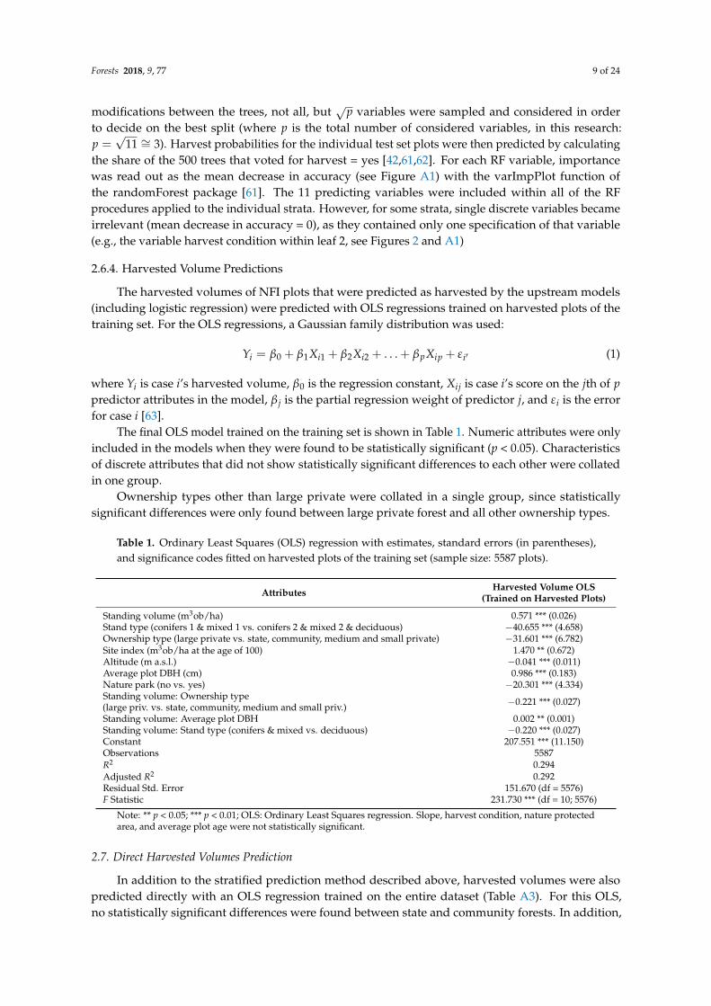
The final OLS model trained on the training set is shown in Table 1. Numeric attributes were onlyincluded in the models when they were found to be statistically significant (p < 0.05). Characteristicsof discrete attributes that did not show statistically significant differences to each other were collatedin one group.

Ownership types other than large private were collated in a single group, since statisticallysignificant differences were only found between large private forest and all other ownership types.

Table 1. Ordinary Least Squares (OLS) regression with estimates, standard errors (in parentheses),and significance codes fitted on harvested plots of the training set (sample size: 5587 plots).

Attributes Harvested Volume OLS(Trained on Harvested Plots)

Standing volume (m3ob/ha) 0.571 *** (0.026)Stand type (conifers 1 & mixed 1 vs. conifers 2 & mixed 2 & deciduous) −40.655 *** (4.658)Ownership type (large private vs. state, community, medium and small private) −31.601 *** (6.782)Site index (m3ob/ha at the age of 100) 1.470 ** (0.672)Altitude (m a.s.l.) −0.041 *** (0.011)Average plot DBH (cm) 0.986 *** (0.183)Nature park (no vs. yes) −20.301 *** (4.334)Standing volume: Ownership type(large priv. vs. state, community, medium and small priv.) −0.221 *** (0.027)

Standing volume: Average plot DBH 0.002 ** (0.001)Standing volume: Stand type (conifers & mixed vs. deciduous) −0.220 *** (0.027)Constant 207.551 *** (11.150)Observations 5587R2 0.294Adjusted R2 0.292Residual Std. Error 151.670 (df = 5576)F Statistic 231.730 *** (df = 10; 5576)

Note: ** p < 0.05; *** p < 0.01; OLS: Ordinary Least Squares regression. Slope, harvest condition, nature protectedarea, and average plot age were not statistically significant.

2.7. Direct Harvested Volumes Prediction

In addition to the stratified prediction method described above, harvested volumes were alsopredicted directly with an OLS regression trained on the entire dataset (Table A3). For this OLS,no statistically significant differences were found between state and community forests. In addition,

Forests 2018, 9, 77 10 of 24

no statistically significant differences were found between the stand types conifers 1 and mixed 1,or between the stand types conifers 2, mixed 2, and deciduous. Furthermore, no differences werefound between small and medium private forests. The respective groups were joined. Average plotage, average plot DBH, harvest condition, and nature protected area were not statistically significant.

2.8. Harvested Decision Prediction with Logistic Regression

A commonly used option would be to use logistic regression to predict harvest occurrencesinstead of the stratified approach. The logistic regression was conducted with a binominal familydistribution, with harvest decision as the response attribute. It can be expressed as:

Pi =1

1 + e−βxi(2)

Pi is the harvest probability of the ith plot within the 10-year period and βx is a linear combinationof parameters (β) and explanatory attributes (x) [21].

When the logistic regression was fit to the training set, no statistically significant differenceswere found between the stand types conifers 1 and mixed 1, or between the stand types conifers 2,mixed 2, and deciduous. For ownership type, no statistically significant differences were foundbetween state and large private forest. The respective groups were joined. The final logistic modelincluded 11 variables and three interactions (see Table A4).

Within the prediction process, the fitted logistic regression was used to predict individual harvestprobabilities at plot level first. To convert harvest probabilities to binary harvest decisions, cut-offs hadto be defined. The definition of cut-off points was derived in an intermediate step using the trainingset. The models were used to predict harvest decisions for the training data. The predictions werethen used in combination with the real NFI harvest decisions to determine cut-off points using the Rpackage OptimalCutpoints [41,53] with max kappa (MK) or the Youden index (YI) as criteria [41,64,65].

Max kappa is based on Cohen’s kappa, which is defined as:

Kp =p1 − p2

1− p2(3)

where p1 is the probability that two classifiers agree, and p2 is the probability that two classifiersagree by chance [55,64]. Since max kappa already resulted in good predictions of overall harvestshares, the Youden index was only used as a criterion to demonstrate the effect of shifting the cut-offbenchmark. It resulted in a cut-off clearly different from max kappa and is defined as [41,65]:

YI(c) = maxc(Sensitivity(c) + Speci f icity(c)− 1) (4)

The derived cut-offs were used to split the predicted probabilities of the test set plots into thecharacteristics yes and no.

OLS trained on harvested plots of the training data only (Table 1, see above) were then applied tothose test set plots predicted as harvested by the upstream logistic models. The harvested volumes oftest set plot predicted as not harvested were set to zero.

3. Results

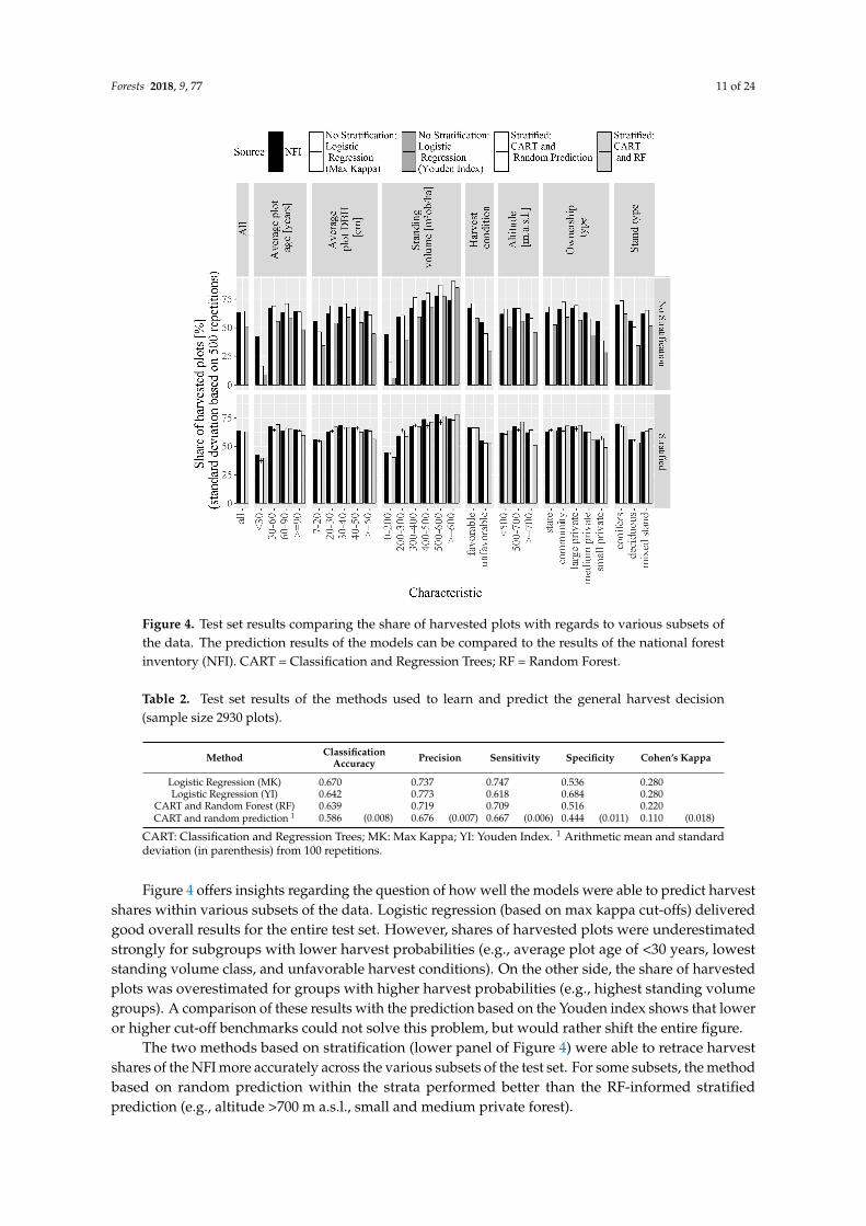
Table 2 and Figure 4 compare the results of the upstream models that were used to predict theharvest occurrence with NFI results. Logistic regression resulted in higher classification accuracieswhen compared to the methods based on stratification (CART). Harvest decisions predicted randomlywithin the strata resulted in the lowest classification accuracies. When the selection within the stratawas informed by RF, accuracy values were closer to, but still below, those of the logistic regression.

Forests 2018, 9, 77 11 of 24Forests 2018, 9, x FOR PEER REVIEW 11 of 24

Figure 4. Test set results comparing the share of harvested plots with regards to various subsets of the data. The prediction results of the models can be compared to the results of the national forest inventory (NFI). CART = Classification and Regression Trees; RF = Random Forest.

Table 2. Test set results of the methods used to learn and predict the general harvest decision (sample size 2930 plots).

Method Classification

Accuracy Precision Sensitivity Specificity Cohen’s Kappa

Logistic Regression (MK) 0.670 0.737 0.747 0.536 0.280 Logistic Regression (YI) 0.642 0.773 0.618 0.684 0.280

CART and Random Forest (RF) 0.639 0.719 0.709 0.516 0.220 CART and random prediction 1 0.586 (0.008) 0.676 (0.007) 0.667 (0.006) 0.444 (0.011) 0.110 (0.018)

CART: Classification and Regression Trees; MK: Max Kappa; YI: Youden Index. 1 Arithmetic mean and standard deviation (in parenthesis) from 100 repetitions.

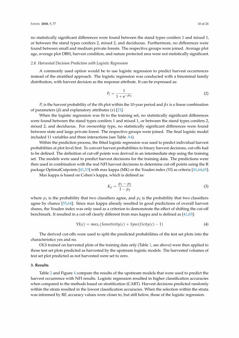
Figure 4 offers insights regarding the question of how well the models were able to predict harvest shares within various subsets of the data. Logistic regression (based on max kappa cut-offs) delivered good overall results for the entire test set. However, shares of harvested plots were underestimated strongly for subgroups with lower harvest probabilities (e.g., average plot age of <30 years, lowest standing volume class, and unfavorable harvest conditions). On the other side, the share of harvested plots was overestimated for groups with higher harvest probabilities (e.g., highest standing volume groups). A comparison of these results with the prediction based on the Youden index shows that lower or higher cut-off benchmarks could not solve this problem, but would rather shift the entire figure.

The two methods based on stratification (lower panel of Figure 4) were able to retrace harvest shares of the NFI more accurately across the various subsets of the test set. For some subsets, the method based on random prediction within the strata performed better than the RF-informed stratified prediction (e.g., altitude >700 m a.s.l., small and medium private forest).

Figure 4. Test set results comparing the share of harvested plots with regards to various subsets ofthe data. The prediction results of the models can be compared to the results of the national forestinventory (NFI). CART = Classification and Regression Trees; RF = Random Forest.

Table 2. Test set results of the methods used to learn and predict the general harvest decision(sample size 2930 plots).

Method ClassificationAccuracy Precision Sensitivity Specificity Cohen’s Kappa

Logistic Regression (MK) 0.670 0.737 0.747 0.536 0.280Logistic Regression (YI) 0.642 0.773 0.618 0.684 0.280

CART and Random Forest (RF) 0.639 0.719 0.709 0.516 0.220CART and random prediction 1 0.586 (0.008) 0.676 (0.007) 0.667 (0.006) 0.444 (0.011) 0.110 (0.018)

CART: Classification and Regression Trees; MK: Max Kappa; YI: Youden Index. 1 Arithmetic mean and standarddeviation (in parenthesis) from 100 repetitions.

Figure 4 offers insights regarding the question of how well the models were able to predict harvestshares within various subsets of the data. Logistic regression (based on max kappa cut-offs) deliveredgood overall results for the entire test set. However, shares of harvested plots were underestimatedstrongly for subgroups with lower harvest probabilities (e.g., average plot age of <30 years, loweststanding volume class, and unfavorable harvest conditions). On the other side, the share of harvestedplots was overestimated for groups with higher harvest probabilities (e.g., highest standing volumegroups). A comparison of these results with the prediction based on the Youden index shows that loweror higher cut-off benchmarks could not solve this problem, but would rather shift the entire figure.

The two methods based on stratification (lower panel of Figure 4) were able to retrace harvestshares of the NFI more accurately across the various subsets of the test set. For some subsets, the methodbased on random prediction within the strata performed better than the RF-informed stratifiedprediction (e.g., altitude >700 m a.s.l., small and medium private forest).

Forests 2018, 9, 77 12 of 24

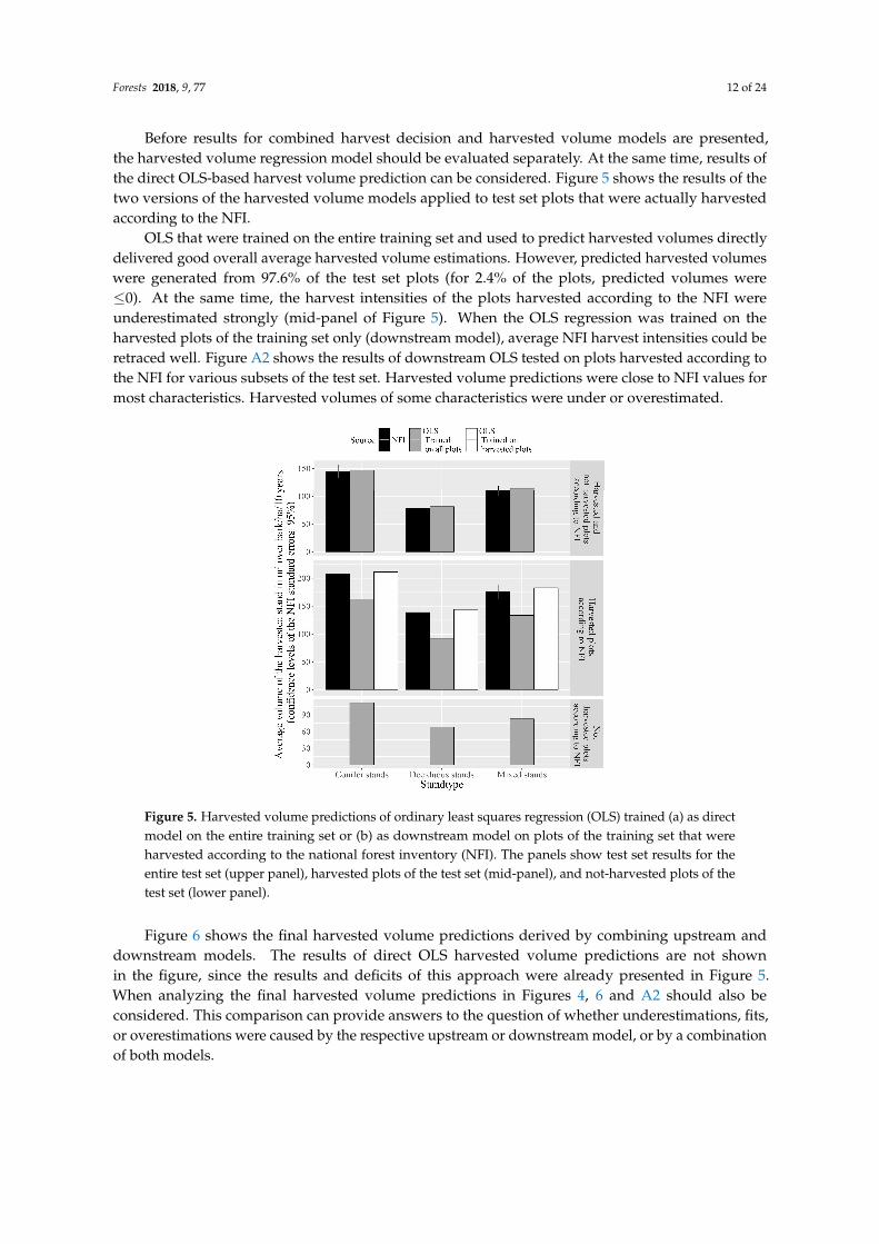
Before results for combined harvest decision and harvested volume models are presented,the harvested volume regression model should be evaluated separately. At the same time, results ofthe direct OLS-based harvest volume prediction can be considered. Figure 5 shows the results of thetwo versions of the harvested volume models applied to test set plots that were actually harvestedaccording to the NFI.

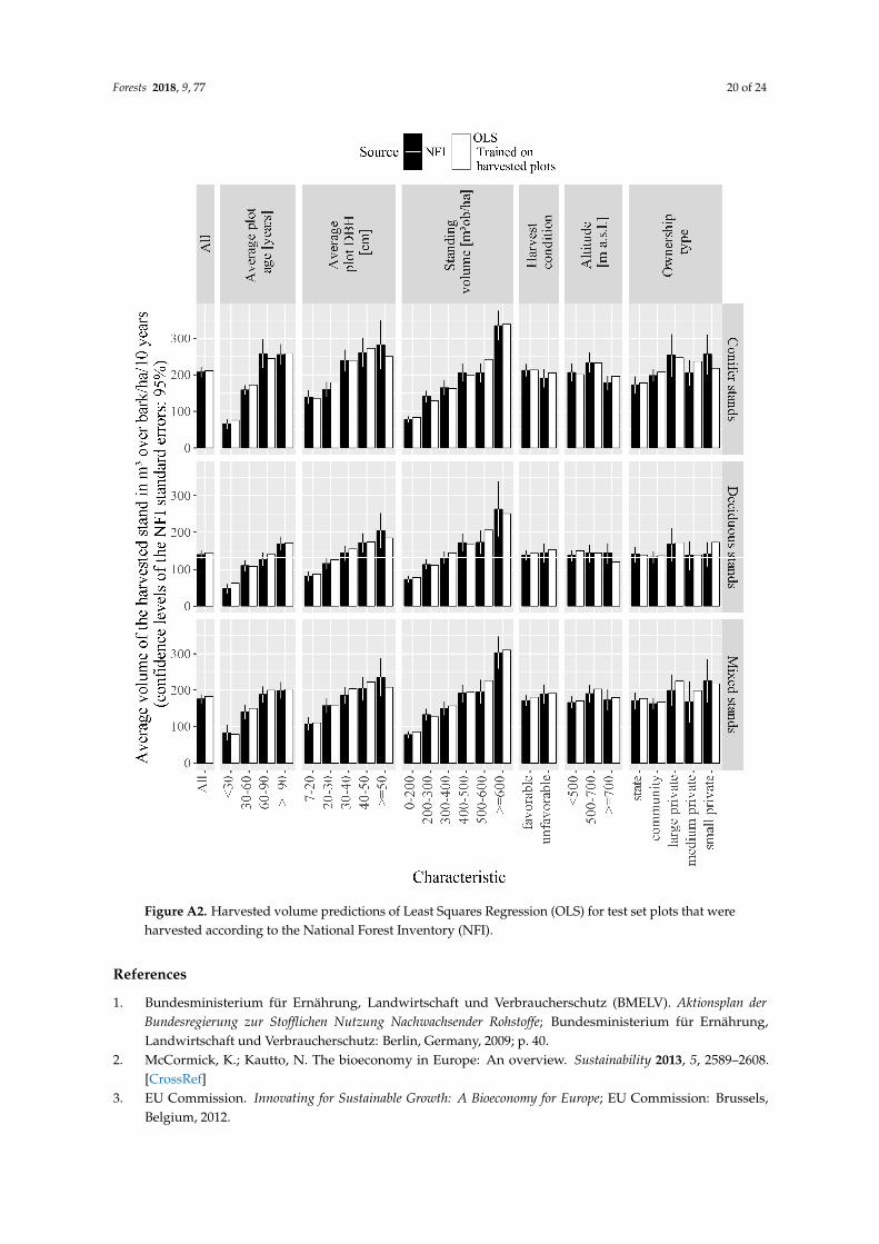
OLS that were trained on the entire training set and used to predict harvested volumes directlydelivered good overall average harvested volume estimations. However, predicted harvested volumeswere generated from 97.6% of the test set plots (for 2.4% of the plots, predicted volumes were≤0). At the same time, the harvest intensities of the plots harvested according to the NFI wereunderestimated strongly (mid-panel of Figure 5). When the OLS regression was trained on theharvested plots of the training set only (downstream model), average NFI harvest intensities could beretraced well. Figure A2 shows the results of downstream OLS tested on plots harvested according tothe NFI for various subsets of the test set. Harvested volume predictions were close to NFI values formost characteristics. Harvested volumes of some characteristics were under or overestimated.

Forests 2018, 9, x FOR PEER REVIEW 12 of 24

Before results for combined harvest decision and harvested volume models are presented, the harvested volume regression model should be evaluated separately. At the same time, results of the direct OLS-based harvest volume prediction can be considered. Figure 5 shows the results of the two versions of the harvested volume models applied to test set plots that were actually harvested according to the NFI.

OLS that were trained on the entire training set and used to predict harvested volumes directly delivered good overall average harvested volume estimations. However, predicted harvested volumes were generated from 97.6% of the test set plots (for 2.4% of the plots, predicted volumes were ≤0). At the same time, the harvest intensities of the plots harvested according to the NFI were underestimated strongly (mid-panel of Figure 5). When the OLS regression was trained on the harvested plots of the training set only (downstream model), average NFI harvest intensities could be retraced well. Figure A2 shows the results of downstream OLS tested on plots harvested according to the NFI for various subsets of the test set. Harvested volume predictions were close to NFI values for most characteristics. Harvested volumes of some characteristics were under or overestimated.

Figure 5. Harvested volume predictions of ordinary least squares regression (OLS) trained (a) as direct model on the entire training set or (b) as downstream model on plots of the training set that were harvested according to the national forest inventory (NFI). The panels show test set results for the entire test set (upper panel), harvested plots of the test set (mid-panel), and not-harvested plots of the test set (lower panel).

Figure 6 shows the final harvested volume predictions derived by combining upstream and downstream models. The results of direct OLS harvested volume predictions are not shown in the figure, since the results and deficits of this approach were already presented in Figure 5. When analyzing the final harvested volume predictions in Figure 6, Figure A2 and Figure 4 should also be considered. This comparison can provide answers to the question of whether underestimations, fits, or overestimations were caused by the respective upstream or downstream model, or by a combination of both models.

Figure 5. Harvested volume predictions of ordinary least squares regression (OLS) trained (a) as directmodel on the entire training set or (b) as downstream model on plots of the training set that wereharvested according to the national forest inventory (NFI). The panels show test set results for theentire test set (upper panel), harvested plots of the test set (mid-panel), and not-harvested plots of thetest set (lower panel).

Figure 6 shows the final harvested volume predictions derived by combining upstream anddownstream models. The results of direct OLS harvested volume predictions are not shownin the figure, since the results and deficits of this approach were already presented in Figure 5.When analyzing the final harvested volume predictions in Figures 4, 6 and A2 should also beconsidered. This comparison can provide answers to the question of whether underestimations, fits,or overestimations were caused by the respective upstream or downstream model, or by a combinationof both models.

Forests 2018, 9, 77 13 of 24Forests 2018, 9, x FOR PEER REVIEW 13 of 24

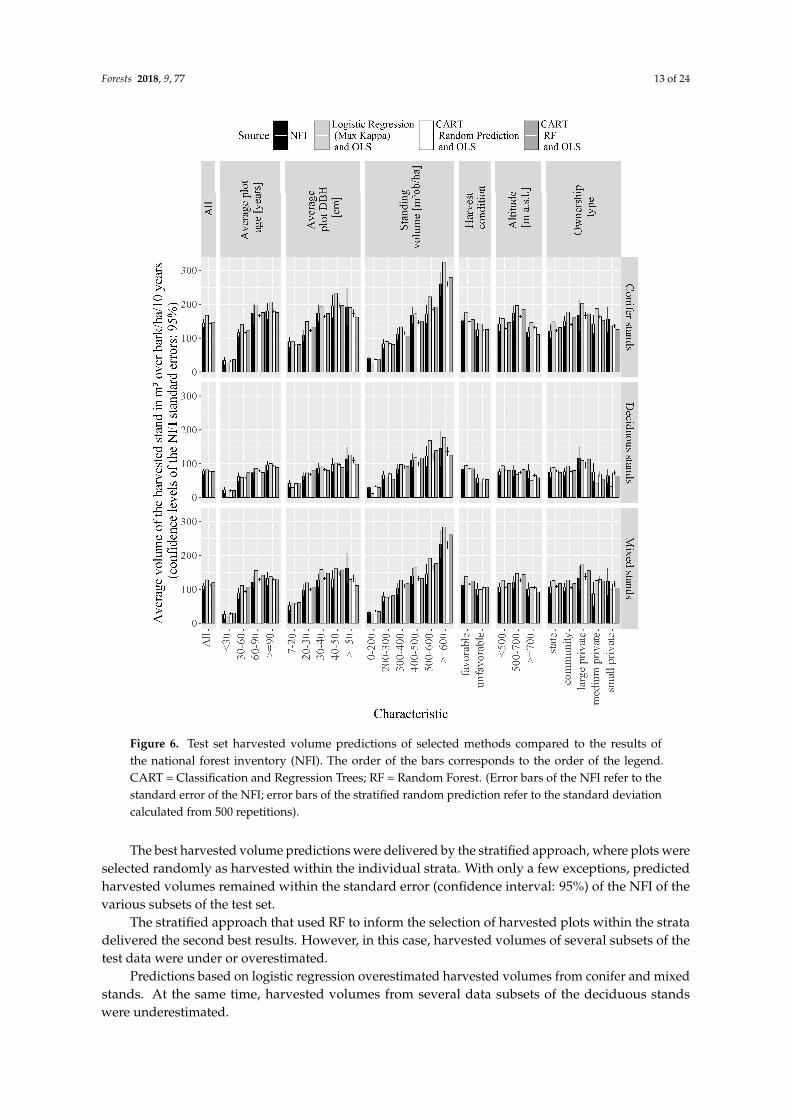
Figure 6. Test set harvested volume predictions of selected methods compared to the results of the national forest inventory (NFI). The order of the bars corresponds to the order of the legend. CART = Classification and Regression Trees; RF = Random Forest. (Error bars of the NFI refer to the standard error of the NFI; error bars of the stratified random prediction refer to the standard deviation calculated from 500 repetitions).

The best harvested volume predictions were delivered by the stratified approach, where plots were selected randomly as harvested within the individual strata. With only a few exceptions, predicted harvested volumes remained within the standard error (confidence interval: 95%) of the NFI of the various subsets of the test set.

The stratified approach that used RF to inform the selection of harvested plots within the strata delivered the second best results. However, in this case, harvested volumes of several subsets of the test data were under or overestimated.

Predictions based on logistic regression overestimated harvested volumes from conifer and mixed stands. At the same time, harvested volumes from several data subsets of the deciduous stands were underestimated.

Figure 6. Test set harvested volume predictions of selected methods compared to the results ofthe national forest inventory (NFI). The order of the bars corresponds to the order of the legend.CART = Classification and Regression Trees; RF = Random Forest. (Error bars of the NFI refer to thestandard error of the NFI; error bars of the stratified random prediction refer to the standard deviationcalculated from 500 repetitions).

The best harvested volume predictions were delivered by the stratified approach, where plots wereselected randomly as harvested within the individual strata. With only a few exceptions, predictedharvested volumes remained within the standard error (confidence interval: 95%) of the NFI of thevarious subsets of the test set.

The stratified approach that used RF to inform the selection of harvested plots within the stratadelivered the second best results. However, in this case, harvested volumes of several subsets of thetest data were under or overestimated.

Predictions based on logistic regression overestimated harvested volumes from conifer and mixedstands. At the same time, harvested volumes from several data subsets of the deciduous standswere underestimated.

Forests 2018, 9, 77 14 of 24

4. Discussion

Research results showed that each of the tested methods had strengths and weaknesses. Logisticregression achieved the highest overall classification accuracies, but overestimated harvest sharesfor some characteristics, while underestimating the harvest shares of others. The stratified methodwith random selection resulted in better prediction of harvest shares, but achieved much lowerharvest accuracies. The RF informed stratified method achieved results in between the logistic andthe stratified random approach. Results are discussed in more detail below, starting with the directharvested volume prediction.

The linear OLS regression that was trained on both harvested and not-harvested plots and usedto predict harvested volumes directly appeared at first glance to deliver good results. However,this approach neglected that a substantial share of NFI plots was not harvested within the 10-yearperiod. Since the absence of logging interventions is part of current business-as-usual, it should alsobe captured in BAU scenarios (compare also Eid [66] cited in Antón-Fernández and Astrup [21]).A related shortcoming is that, on average, harvested plots were in reality treated with considerablyhigher harvest intensities than predicted by the directly applied models. Using the direct approachto predict future wood supply might result in adequate business-as-usual overall quantities for thefirst decade. However, instead of realizing these harvested volumes from around 65% of the plots,the direct model would harvest these quantities from nearly 100% of the plots treated with comparablylow intensities. Thus, the prediction would result in a forest inventory structure that is clearly differentfrom business-as-usual at the end of the decade. This direct approach would be especially unsuitablefor projection periods longer than 10 years.

However, it was also shown that the OLS was able to predict the harvested volumes of harvestedNFI plots well when trained and tested on subsets of harvested plots only (the downstream model).To make use of these versions of the model in a BAU scenario, it was necessary to first predict theoccurrence or non-occurrence of harvest interventions.

Logistic regression is a common approach for binary decision problems [21,36]. In the context ofthis research, it delivered better results than the tested stratified methods with regards to classificationaccuracy, precision, specificity, and Cohen’s kappa. Nevertheless, the logistic regression failed to predictaccurate harvest shares for several subsets of the test set. When combined with the downstream OLSmodel, the logistic model resulted in overestimations of harvested volumes for some characteristics,and underestimations of others. This problem is directly linked to only one overall benchmark beingused to convert the predicted harvest probabilities into the decision yes or no. Predicting harvestoccurrences from CART with an overall cut-off would create similar problems.

Logistic regression resulted in higher, but—at least in the case of this research—not sufficientlyhigh classification accuracies. An important factor here is the noisiness of the large-scale inventorydata. The forest area based on which an owner or manager makes a harvest decision might lookdifferent from what is suggested by the inventory plot. With the exception of selection (plenter) felling,a harvest decision is usually made for an area (e.g., a forest stand or a section of a forest stand). In thecase of the German NFI, only one or two inventory plots might be found per included decision area.However, a higher number of plots would be needed in order to produce a representative picture ofthat area [67].

The most accurate way of designing BAU wood supply scenarios would be to generate modelswith high classification accuracies. However, if this is not feasible (e.g., due to data noise) an alternativeis to design models that deliver accurate harvest proportions throughout subsets of the dataset.The stratified prediction methods tested in the scope of this research can be used to optimize the modeltowards this goal.

In this research, CART was used for the stratification process. However, comparable stratifyingmachine learning algorithms such as C.45 [68] might also be applicable for this purpose. The CARTalgorithm divided NFI plots of the training set into strata, and delivered common harvest probabilitiesfor each stratum. The fitted CART could then be applied to the test set. The algorithm assigned the test

Forests 2018, 9, 77 15 of 24

set NFI plots to the respective stratum where corresponding probabilities (derived from the trainingset) could be used to select an adequate proportion of the test set plots as harvested. Thus, instead ofassuming that plots with harvest probabilities of 20% were not harvested at all (as done by the cut-offmethod), it was possible to select 20% of these plots as harvested. The question is now: which of theplots should be selected as harvested?

In a first approach, it was simply assumed that no further factors, but rather only noise, influencedthe harvest decision at the plot level, and plots were selected randomly as harvested according to thespecific harvest probability of a stratum. This approach resulted in good predictions of harvest sharesand harvested volume across the various subsets of the test set. An important drawback was that theclassification accuracy, precision, specificity, and Cohen’s kappa values dropped considerably whencompared to the cut-off approach. Furthermore, it was necessary to repeat the procedure and averageoutcomes of the repetition.

In a second approach, a RF algorithm was used to inform the selection of harvested plots withinthe various strata. In this way, each NFI plot within the test set obtained an additional individualharvest probability. Again, shares of plots corresponding to the harvest probabilities of specific stratawere selected. However, this time, the plots with the highest individual harvest probabilities wereselected first, and the selection stopped as soon as the respective harvest share of the stratum wasreached. Harvest share predictions were comparable to the results of the random approach. However,for some subsets (e.g., plots above 700 m a.s.l., plots above 50-cm average DBH, and small privateforest plots), the random selection delivered better results. At the same time, classification accuracy,precision, specificity, and kappa values increased considerably, but still remained below the results ofthe logistic models.

With reference to factors impacting harvest decisions, the outcome of this research mostlyconfirmed the results of previous research. Harvest condition and slope [21,38,50] were found tohave impacts on the general decision about whether or not a plot is harvested. These factors were notfound to influence the harvest intensity once this decision was made. However, it is possible that plotswith more difficult harvest conditions are harvested less frequently, but with higher intensity, and thatthis pattern is blurred due to the given period of 10 years. The factor ownership type [17,18,37] was alsofound to have important impacts. An interesting finding was that, for harvest occurrence, differenceswere found between community, state, and large private forests (as one group), medium private forests,and small private forests (with decreasing harvest probability across the groups listed from first to last,see Table A4). However, only the large private forest was found to be harvested at higher intensities.No differences in harvest intensities could be found between the other ownership types.

A restriction of the research is that the results remain on a relatively broad level as concernstimber species and dimensions. Instead of referring to individual timber species, plot level standtypes grouped into five broad groups were used. Included dimension information referred to averagevalues for the NFI plots. However, results of this research could be used to integrate BAU scenariosinto AFGWSMs, where results could be further broken down to individual tree levels and even thecomputation of timber assortments would be possible [43,69].

The available information for NFI plots was dominated by stand or site-specific attributes.With regards to the human factor, only rough information on ownership type and property sizeswas available. The objectives and behavior of NIPF owners are considered to be heterogeneous,dynamic, and complex [29,70–74]. However, given this complexity, and the fact that NFI plots are notrepresentative of decision areas, it is unclear in how far more ownership-specific information wouldhelp to improve the accuracies of the models.

Within the reference period, business-as-usual procedures were disturbed by storms and a droughtperiod. Here, it should be asked how far and to what degree of severity natural disturbances shouldbe considered as part of usual business. For instance, bark beetle impacts related to elevation andtimber dimensions as described by Sterba et al. [33] might, for example, still be considered normal.In contrast, Seidl et al. [75] dedicated a study to the projection of bark beetle disturbances in the context

Forests 2018, 9, 77 16 of 24

of climate change impacts and adaptive management strategies. This can be considered as divergingfrom business-as-usual. Within the German NFI, the specific timing of and reason for tree harvests arenot recorded. Furthermore, the occurrence of salvage fellings is likely to impact other harvest decisions.Thus, in any case, it would be difficult to deduct harvest occurrences caused by disturbances.

Plots of the German NFI are not representative of the stands or decision areas in which theyare located. The non-occurrence of harvest interventions on an NFI plot does not imply that theentire stand was not harvested and vice versa. Thus, it has to be kept in mind that a BAU scenariogenerated with the presented method is, first of all, a projection of the NFI. However, the NFI isconsidered a random sampling (by neglecting the systematic arrangement of the tracts) [46] thatdelivers representative and valid data on forest conditions on a larger scale [8].

CART turned out to be a valuable tool for the stratified prediction. An additional advantageis that the algorithm resulted in a classification tree that can be easily interpreted. In this context,Domingos [57] (p. 2) argues: “[ . . . ] it is not enough for a learned model to be accurate; it alsoneeds to be understood by its human users, if they are to trust it and deem it acceptable”. However,a disadvantage of CART is its instability [57]. Setting the minimum number of observations perterminal leaf to 100 and pruning the tree helped to gain more stability and avoid over-fitting.Nevertheless, smaller changes in the input data could still result in different tree structures. However,alternative algorithms that could be used for stratification such as C4.5 [68] have similar issues [55,57]and more stable methods such as RF are unsuitable for the stratification process.

5. Conclusions

It can be summarized that the stratified method generated good results. Among the group oftested prediction methods and under the given data conditions and restrictions, it can be consideredas the most suitable for generating BAU timber supply scenarios. The direct prediction of harvestedvolumes with a linear regression trained on both harvested and not-harvested NFI plots is not an option,since this method resulted in harvesting patterns that were clearly different from BAU. Using logisticregression with an overall cut-off benchmark resulted in strong harvested volume overestimationsfor some characteristics, and underestimations for others. A trade-off of the stratified method is thedecrease in classification accuracy and related quality measures. However, when the selection of plotsto be harvested was not generated randomly, but rather informed by RF, this impairment remainedwithin an acceptable range. Furthermore, in the scope of large-scale timber supply projections, it mightbe considered as more important to find the right number of harvested plots than to identify thoseplots that were actually harvested.

Results of this research must be interpreted in respect of the regional and periodical backgroundconditions, the data quality of the German NFI, and the availability of attributes that could be used andlinked to the NFI data. However, considering that large-scale forest inventories are often rather noisy,the presented stratified methods could also be helpful for generating useful BAU forest developmentand wood supply scenarios in other regions.

The stratified method should be tested and challenged when applied to other time periods,regions, and inventory variations. A further challenge is to combine this method with AFGWSMs togenerate BAU scenarios for forest development and timber supply projections beyond one decade.In this context, another challenge is to learn and predict BAU harvesting choices for individual trees.The results of this research showed that BAU harvesting patterns could be retraced well without havingmore detailed background information on individual harvest decisions. However, the parametrizedBAU scenario could also be used as a baseline for the design of alternative scenarios. For this purpose,underlying social and economic grounds for harvest choices would have to be studied specifically inrelation to inventory based scenario design. More research explicitly dedicated to this task is needed.

Acknowledgments: This work was supported by a grant from the Ministry of Science, Research and theArts of Baden-Württemberg and the Baden-Württemberg Stiftung Az: 33-7533-10-5. The article processingcharge was funded by the German Research Foundation (DFG) and the University of Freiburg in the funding

Forests 2018, 9, 77 17 of 24

program Open Access Publishing. We would like to thank Emily Kilham for copyediting and proofreading thispaper. Furthermore, we want to thank Jürgen Bauhus, Gregor Nagel, Reinhard Aichholz, Sebastian Schmack,Joachim Maack, and Dominik Cullmann for valuable feedback, and Uli Riemer, Niclas Aleff, Diana Boada,Lisa Rummel, and Juliane Herpich for their supportive work.

Author Contributions: Philipp Kilham: Development of study, data analysis, and writing of manuscript.Gerald Kändler: Coordination, development of study and improvement of manuscript. Christoph Hartebrodt:Coordination and development of study. Anne-Sophie Stelzer: Improvement of data analysis and manuscript.Ulrich Schraml: Revision and improvement of manuscript.

Conflicts of Interest: The authors declare no conflict of interest. The founding sponsors had no role in the designof the study; in the collection, analyses, or interpretation of data; in the writing of the manuscript, and in thedecision to publish the results.

Appendix A

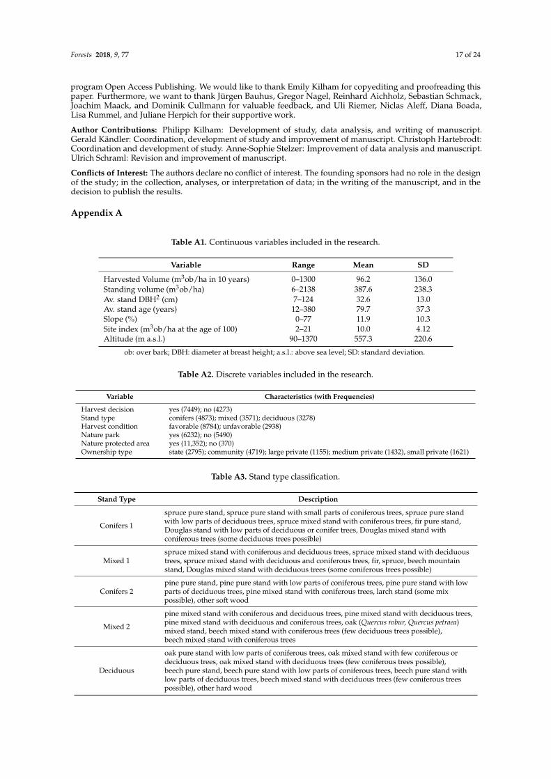
Table A1. Continuous variables included in the research.

Variable Range Mean SD

Harvested Volume (m3ob/ha in 10 years) 0–1300 96.2 136.0Standing volume (m3ob/ha) 6–2138 387.6 238.3Av. stand DBH2 (cm) 7–124 32.6 13.0Av. stand age (years) 12–380 79.7 37.3Slope (%) 0–77 11.9 10.3Site index (m3ob/ha at the age of 100) 2–21 10.0 4.12Altitude (m a.s.l.) 90–1370 557.3 220.6

ob: over bark; DBH: diameter at breast height; a.s.l.: above sea level; SD: standard deviation.

Table A2. Discrete variables included in the research.

Variable Characteristics (with Frequencies)

Harvest decision yes (7449); no (4273)Stand type conifers (4873); mixed (3571); deciduous (3278)Harvest condition favorable (8784); unfavorable (2938)Nature park yes (6232); no (5490)Nature protected area yes (11,352); no (370)Ownership type state (2795); community (4719); large private (1155); medium private (1432), small private (1621)

Table A3. Stand type classification.

Stand Type Description

Conifers 1

spruce pure stand, spruce pure stand with small parts of coniferous trees, spruce pure standwith low parts of deciduous trees, spruce mixed stand with coniferous trees, fir pure stand,Douglas stand with low parts of deciduous or conifer trees, Douglas mixed stand withconiferous trees (some deciduous trees possible)

Mixed 1spruce mixed stand with coniferous and deciduous trees, spruce mixed stand with deciduoustrees, spruce mixed stand with deciduous and coniferous trees, fir, spruce, beech mountainstand, Douglas mixed stand with deciduous trees (some coniferous trees possible)

Conifers 2pine pure stand, pine pure stand with low parts of coniferous trees, pine pure stand with lowparts of deciduous trees, pine mixed stand with coniferous trees, larch stand (some mixpossible), other soft wood

Mixed 2

pine mixed stand with coniferous and deciduous trees, pine mixed stand with deciduous trees,pine mixed stand with deciduous and coniferous trees, oak (Quercus robur, Quercus petraea)mixed stand, beech mixed stand with coniferous trees (few deciduous trees possible),beech mixed stand with coniferous trees

Deciduous

oak pure stand with low parts of coniferous trees, oak mixed stand with few coniferous ordeciduous trees, oak mixed stand with deciduous trees (few coniferous trees possible),beech pure stand, beech pure stand with low parts of coniferous trees, beech pure stand withlow parts of deciduous trees, beech mixed stand with deciduous trees (few coniferous treespossible), other hard wood

Forests 2018, 9, 77 18 of 24

Table A4. Used regression models with estimates, standard errors (in parentheses), and significancecodes fitted on the entire training dataset (sample size: 8792 plots).

Attributes Harvest DecisionLogistic Regression

HarvestedVolume OLS

Standing volume (m3/ha) 0.004 *** (0.000) 0.532 *** (0.019)Stand type (conifers 1 & mixed 1 vs. conifers 2 & mix. 2 & deciduous) −0.383 *** (0.068) −43.547 *** (4.480)Ownership type (small private vs. community) 1.023 *** (0.075)Ownership type (small private vs. state and large priv.) 0.866 *** (0.077)Ownership type (small private vs. medium priv.) 0.496 *** (0.093)Ownership type (large private vs. state, and community) −25.177 *** (5.294)Ownership type (large private vs. medium and small private) −46.713 *** (5.854)Harvest condition (favorable vs. unfavorable) −0.376 *** (0.074)Site index (m3ob/ha at the age of 100) −0.018 ** (0.009) 1.909 *** (0.497)Altitude (m a.s.l.) −0.001 *** (0.000) −0.041 *** (0.008)Slope (%) −0.015 *** (0.003) −1.053 *** (0.161)Average plot DBH (cm) −0.01 *** (0.003)Average plot age (years) −0.004 *** (0.001)Nature park (no vs. yes) −0.179 *** (0.054) −17.257 *** (3.440)Nature protected area (no vs. yes) −0.633 *** (0.137)Standing volume: Ownership type (other vs. small or medium private) −0.001 *** (0.000)Standing volume: Ownership type (large private vs. state, and community) −0.126 *** (0.021)Standing volume: Ownership type (large private vs. medium and small private) −0.224 *** (0.022)Standing volume: Average plot DBH 0.001 ** (0.001)Standing volume: Stand type(conifers 1 & mixed 1 vs. deciduous & conifers 2 & mix. 2) −0.156 *** (0.014)

Standing volume: Average plot age −0.000 *** (0.000)Average plot Age: Average plot DBH 0.000 *** (0.000)Constant 0.410 *** (0.078) 154.412 *** (8.359)Observations 8792 8792R2 0.278Adjusted R2 0.277Log Likelihood −5134.677Akaike Inf. Crit. 10,303.350Residual Std. Error 144.740 (df = 8779)F Statistic 281.502 *** (df = 12; 8779)

Note: *p < 0.05; ** p < 0.01; OLS: Ordinary least squares regression.

Forests 2018, 9, 77 19 of 24Forests 2018, 9, x FOR PEER REVIEW 19 of 24

Figure A1. Variable importance for Random Forests applied to individual leaves of the classification tree.

Figure A1. Variable importance for Random Forests applied to individual leaves of theclassification tree.

Forests 2018, 9, 77 20 of 24Forests 2018, 9, x FOR PEER REVIEW 20 of 24

Figure A2. Harvested volume predictions of Least Squares Regression (OLS) for test set plots that were harvested according to the National Forest Inventory (NFI).

References

1. Bundesministerium für Ernährung, Landwirtschaft und Verbraucherschutz (BMELV). Aktionsplan der Bundesregierung zur Stofflichen Nutzung Nachwachsender Rohstoffe; Bundesministerium für Ernährung, Landwirtschaft und Verbraucherschutz: Berlin, Germany, 2009; p. 40.

2. McCormick, K.; Kautto, N. The bioeconomy in Europe: An overview. Sustainability 2013, 5, 2589–2608, doi:10.3390/su5062589.

3. EU Commission. Innovating for Sustainable Growth: A Bioeconomy for Europe; EU Commission: Brussels, Belgium, 2012.

Figure A2. Harvested volume predictions of Least Squares Regression (OLS) for test set plots that wereharvested according to the National Forest Inventory (NFI).

References

1. Bundesministerium für Ernährung, Landwirtschaft und Verbraucherschutz (BMELV). Aktionsplan derBundesregierung zur Stofflichen Nutzung Nachwachsender Rohstoffe; Bundesministerium für Ernährung,Landwirtschaft und Verbraucherschutz: Berlin, Germany, 2009; p. 40.

2. McCormick, K.; Kautto, N. The bioeconomy in Europe: An overview. Sustainability 2013, 5, 2589–2608.[CrossRef]

3. EU Commission. Innovating for Sustainable Growth: A Bioeconomy for Europe; EU Commission: Brussels,Belgium, 2012.

Forests 2018, 9, 77 21 of 24

4. Vauhkonen, J.; Packalen, T. A Markov Chain Model for Simulating Wood Supply from Any-Aged ForestManagement Based on National Forest Inventory (NFI) Data. Forests 2017, 8, 307. [CrossRef]

5. Raunikar, R.; Buongiorno, J.; Turner, J.A.; Zhu, S. Global outlook for wood and forests with the bioenergydemand implied by scenarios of the Intergovernmental Panel on Climate Change. For. Policy Econ. 2010, 12,48–56. [CrossRef]

6. Food and Agriculture Organization (FAO). Emerging Approaches to Forest Reference Emission Levels and/or ForestReference Levels for REDD+; 978-92-5-108840-1; Food and Agriculture Organization of the United Nations:Rome, Italy, 2015.

7. Olander, L.P.; Gibbs, H.K.; Steininger, M.; Swenson, J.J.; Murray, B.C. Reference scenarios for deforestationand forest degradation in support of REDD: A review of data and methods. Environ. Res. Lett. 2008, 3,025011. [CrossRef]

8. Kändler, G. The design of the second German national forest inventory. In Proceedings of the Eighth AnnualForest Inventory and Analysis Symposium, Monterey, CA, USA, 16–19 October 2006; McRoberts, R.E.,Reams, G.A., Van Duesen, P.C., McWilliams, W.H., Eds.; U.S. Department of Agriculture: Washington, DC,USA, 2006; pp. 19–24.

9. Tomppo, E.; Schadauer, K.; McRoberts, R.E.; Gschwantner, T.; Gabler, K.; Ståhl, G. Introduction.In National Forest Inventories: Pathways for Common Reporting; Tomppo, E., Gschwantner, T., Lawrence, M.,McRoberts, R.E., Eds.; Springer: Dordrecht, The Netherlands, 2010; pp. 1–18.

10. Fischer, C.; Gasparini, P.; Nylander, M.; Redmond, J.; Hernandez, L.; Brändli, U.-B.; Pastor, A.; Rizzo, M.;Alberdi, I. Joining Criteria for Harmonizing European Forest Available for Wood Supply Estimates.Case Studies from National Forest Inventories. Forests 2016, 7, 104. [CrossRef]

11. Barreiro, S.; Schelhaas, M.-J.; Kändler, G.; Antón-Fernández, C.; Colin, A.; Bontemps, J.-D.; Alberdi, I.;Condés, S.; Dumitru, M.; Ferezliev, A.; et al. Overview of methods and tools for evaluating future woodybiomass availability in European countries. Ann. For. Sci. 2016, 73, 823–837. [CrossRef]

12. Rock, J.; Gerber, K.; Klatt, S.; Oehmichen, K. Das WEHAM 2012 “Basisszenario”: Mittellinie oderLeitplanke?—The WEHAM 2012 “Baseline scenario”: Center line or guardrail? Forstarchiv 2016, 87, 66–69.

13. Mahmoud, M.; Liu, Y.; Hartmann, H.; Stewart, S.; Wagener, T.; Semmens, D.; Stewart, R.; Gupta, H.;Dominguez, D.; Dominguez, F. A formal framework for scenario development in support of environmentaldecision-making. Environ. Model. Softw. 2009, 24, 798–808. [CrossRef]

14. Intergovernmental Panel on Climate Change (IPPC). Available online: http://www.ipcc-data.org/guidelines/pages/definitions.html (accessed on 7 September 2017).

15. Rounsevell, M.D.A.; Metzger, M.J. Developing qualitative scenario storylines for environmental changeassessment. Wires Clim. Chang. 2010, 1, 606–619. [CrossRef]

16. Wear, D.N.; Parks, P.J. The economics of timber supply: An analytical synthesis of modeling approaches.Nat. Resour. Model. 1994, 8, 199–223. [CrossRef]

17. Polyakov, M.; Wear, D.N.; Huggett, R.N. Harvest choice and timber supply models for forest forecasting.For. Sci. 2010, 56, 344–355.

18. Rinaldi, F.; Jonsson, R.; Sallnäs, O.; Trubins, R. Behavioral modelling in a decision support system. Forests2015, 6, 311–327. [CrossRef]

19. Rinaldi, F.; Jonsson, R. Risks, information and short-run timber supply. Forests 2013, 4, 1158–1170. [CrossRef]20. Henderson, J.D.; Abt, R.C. An agent-based model of heterogeneous forest landowner decisionmaking.

For. Sci. 2016, 62, 364–376. [CrossRef]21. Antón-Fernández, C.; Astrup, R. Empirical harvest models and their use in regional business-as-usual

scenarios of timber supply and carbon stock development. Scand. J. For. Res. 2012, 27, 379–392. [CrossRef]22. Amacher, G.S.; Conway, M.C.; Sullivan, J. Econometric analyses of nonindustrial forest landowners: Is there

anything left to study? J. For. Econ. 2003, 9, 137–164. [CrossRef]23. Beach, R.H.; Pattanayak, S.K.; Yang, J.-C.; Murray, B.C.; Abt, R.C. Econometric studies of non-industrial

private forest management: A review and synthesis. For. Policy Econ. 2005, 7, 261–281. [CrossRef]24. Favada, I.M.; Kuuluvainen, J.; Uusivuori, J. Consistent estimation of long-run nonindustrial private forest

owner timber supply using micro data. Can. J. For. Res. 2007, 37, 1485–1494. [CrossRef]25. Kuuluvainen, J.; Karppinen, H.; Ovaskainen, V. Landowner objectives and nonindustrial private timber

supply. For. Sci. 1996, 42, 300–309.

Forests 2018, 9, 77 22 of 24

26. Vokoun, M.; Amacher, G.S.; Wear, D.N. Scale of harvesting by non-industrial private forest landowners.J. For. Econ. 2006, 11, 223–244. [CrossRef]

27. Koch, S.P.; Schwarzbauer, P.; Stern, T. Monthly wood supply behavior of associated forest owners inAustria—Insights from the analysis of a micro-econometric panel. J. For. Econ. 2013, 19, 331–346. [CrossRef]

28. Bolkesjø, T.F.; Solberg, B. A Panel Data Analysis of Nonindustrial Private Roundwood Supply with Emphasison the Price Elasticity. For. Sci. 2003, 49, 530–538.

29. Butler, B.J.; Hewes, J.H.; Dickinson, B.J.; Andrejczyk, K.; Butler, S.M.; Markowski-Lindsay, M. Family ForestOwnerships of the United States, 2013: Findings from the USDA Forest Service’s National Woodland OwnerSurvey. J. For. 2016, 114, 638–647. [CrossRef]

30. Bolkesjø, T.F.; Solberg, B.; Wangen, K.R. Heterogeneity in nonindustrial private roundwood supply: Lessonsfrom a large panel of forest owners. J. For. Econ. 2007, 13, 7–28. [CrossRef]

31. Silver, E.J.; Leahy, J.E.; Weiskittel, A.R.; Noblet, C.L.; Kittredge, D.B. An Evidence-Based Review of TimberHarvesting Behavior among Private Woodland Owners. J. For. 2015, 113, 490–499. [CrossRef]

32. Tomppo, E.; Gschwantner, T.; Lawrence, M.; McRoberts, R.E. National Forest Inventories: Pathways for CommonReporting; Springer: Dordrecht, The Netherlands, 2010; p. 607.

33. Sterba, H.; Golser, M.; Schadauer, K. Evaluating a model to predict timber harvesting in Austria. In IntegratedTools for Natural Resources Inventories in the 21st Century. General Technical Report NC-212; Hansen, M., Burk, T.,Eds.; USDA Forest Service North Central Forest Experiment Station: Saint Paul, MN, USA, 2000; pp. 569–604.

34. Nabuurs, G.-J.; Schelhaas, M.-J.; Pussinen, A. Validation of the European Forest Information Scenario Model(EFISCEN) and a projection of Finnish forests. Silva Fenn. 2000, 34, 167–179. [CrossRef]

35. Thürig, E.; Schelhaas, M.-J. Evaluation of a large-scale forest scenario model in heterogeneous forests: A casestudy for Switzerland. Can. J. For. Res. 2006, 36, 671–683. [CrossRef]

36. Dennis, D.F. A probit analysis of the harvest decision using pooled time-series and cross-sectional data.J. Environ. Econ. Manag. 1990, 18, 176–187. [CrossRef]

37. Prestemon, J.P.; Wear, D.N. Linking harvest choices to timber supply. For. Sci. 2000, 46, 377–389.38. Verkerk, P.J.; Levers, C.; Kuemmerle, T.; Lindner, M.; Valbuena, R.; Verburg, P.H.; Zudin, S. Mapping wood

production in European forests. For. Ecol. Manag. 2015, 357, 228–238. [CrossRef]39. Zhang, D.; Sun, X.; Butler, B.J.; Prestemon, J.P. Harvesting Choices and Timber Supply among Landowners

in the Southern United States. Can. J. Agric. Econ. 2015, 63, 409–429. [CrossRef]40. Breiman, L.; Friedman, J.; Olshen, R.; Stone, C. Classification and Regression Trees; Taylor & Franxis Group,

LLC: Boca Raton, FL, USA, 1984.41. López-Ratón, M.; Rodríguez-Álvarez, M.X.; Cadarso-Suárez, C.; Gude-Sampedro, F. OptimalCutpoints:

An R Package for Selecting Optimal Cutpoints in Diagnostic Tests. J. Stat. Softw. 2014, 61, 36. [CrossRef]42. Breiman, L. Random Forests. Mach. Learn. 2001, 45, 5–32. [CrossRef]43. Kändler, G.; Riemer, U. Chapter 14—Germany. In Forest Inventory-Based Projection Systems for Wood and

Biomass Availability; Barreiro, S., Schelhaas, M.J., McRoberts, R.E., Kändler, G., Eds.; Springer: Cham,Switzerland, 2017; pp. 175–183.

44. Thünen Institut (TI). Dritte Bundeswaldinventur (2012). Available online: https://bwi.info/ (accessed on8 July 2017).

45. Ministerium für Ländlichen Raum (MLR). Clusterstudie Forst und Holz Baden-Württemberg—Analyse derSpezifischen Wettbewerbssituation des Clusters Forst und Holz und Ableitung von Handlungsempfehlungen;Ministerium für Ländlichen Raum und Verbraucherschutz Baden-Württemberg: Stuttgart, Germany, 2010;p. 177.

46. Schmitz, F.; Polley, H.; Henning, P.; Dunger, K.; Schwitzgebel, F. Die zweite Bundeswaldinventur BWI 2: Inventur-und Auswertungsmethoden—The Second National Forest Inventory NFI 2: Inventory and Evaluation Methods;Bundesministerium für Ernährung, Landwirtschaft und Verbraucherschutz (BMELV): Braunschweig,Germany, 2008; p. 85.

47. Bundesministerium für Ernährung, Landwirtschaft und Verbraucherschutz (BMELV). Aufnahmeanweisungfür die Dritte Bundeswaldinventur (BWI 3) (2011–2012); BMELV: Bonn, Germany, 2011; p. 111.

48. Sloboda, B.; Gaffrey, D.; Matsumura, N. Regionale und lokale Systeme von Höhenkurven für gleichaltrigeWaldbestände. Allg. For. Jagdztg. 1993, 164, 225–228.

Forests 2018, 9, 77 23 of 24

49. Ministerium für Ländlichen Raum (MLR). Hilfstabellen für die Forsteinrichtung; MLR: Stuttgart, Germany,1993; p. 188.

50. Wenzelides, M.; Hagemann, H. Bestimmung des nachhaltig mobilisierbaren Dendromassepotenzials inNordrhein-Westfalen anhand der Auswertung von Bundes-und Landeswaldinventur. Forstarchiv 2007, 78,73–81.

51. Selter, A.; Hartebrodt, C.; Brandl, H.; Herbohn, J. A critical comparison of typologies of small-scale forestryin Baden-Württemberg derived using single and multiple criteria. Small-Scale For. 2009, 8, 25–42. [CrossRef]

52. Kuhn, M. Building predictive models in R using the caret package. J. Stat. Softw. 2008, 28, 1–26. [CrossRef]53. R-Core-Team. R: A Language and Environment for Statistical Computing, version 3.1.1; R Foundation for

Statistical Computing: Vienna, Austria, 2014.54. Hastie, T.; Tibshirani, R.; Friedman, J.; Hastie, T.; Friedman, J.; Tibshirani, R. The Elements of Statistical Learning;

Springer: New York, NY, USA, 2013; Volume 10.55. Zhou, Z.-H. Ensemble Methods—Foundations and Algorithms; CRC Press: Boca Raton, FL, USA, 2012.56. Negnevitsky, M. Artificial Intelligence—A Guide to Intelligent Systems; Pearson Education Limited: Harlow,

UK, 2002; Volume 2.57. Domingos, P. Knowledge discovery via multiple models. Intell. Data Anal. 1998, 2, 187–202. [CrossRef]58. Therneau, T.; Atkinson, B.; Ripley, B. Rpart: Recursive Partitioning and Regression Trees, R Package

Version 4.1-11. Available online: https://cran.r-project.org/web/packages/rpart/index.html (accessed on9 November 2017).

59. Therneau, T.; Atkinson, B.; Ripley, B. Documentation for Package ‘Rpart’ Version 4.1-11. Available online:https://stat.ethz.ch/R-manual/R-devel/library/rpart/html/00Index.html (accessed on 9 November 2017).

60. Kabacoff, R.I. Quick-R. Available online: https://www.statmethods.net/advstats/cart.html (accessed on9 November 2017).

61. Liaw, A.; Matthew, W. Classification and Regression by randomForest. R News 2002, 2, 18–22.62. Liaw, A.; Wiener, M. Package ‘randomForest’—Breiman and Cutler’s Random Forest for Classification,

Version 4.6-12. Available online: https://cran.r-project.org/web/packages/randomForest/randomForest.pdf (accessed on 22 November 2017).

63. Hayes, A.F.; Cai, L. Using heteroskedasticity-consistent standard error estimators in OLS regression:An introduction and software implementation. Behav. Res. Methods 2007, 39, 709–722. [CrossRef] [PubMed]

64. Cohen, J. A Coefficient of Agreement for Nominal Scales. Educ. Psychol. Meas. 1960, 20, 37–46. [CrossRef]65. Youden, W.J. Index for rating diagnostic tests. Cancer 1950, 3, 32–35. [CrossRef]66. Eid, T. Testing a large-scale forestry scenario model by means of successive inventories on a forest property.

Silva Fenn. 2004, 38, 305–317. [CrossRef]67. Kramer, H.; Akça, A. Leitfaden zur Waldmesslehre; J. D. Sauerländers Verlag: Frankfurt, Germany, 2008;

Volume 5, p. 226.68. Quinlan, J.R. C4.5—Programs for Machine Learning; Morgan Kaufmann: San Francisco, CA, USA, 1993.69. Rock, J.; Bösch, B.; Kändler, G. WEHAM 2012—Waldentwicklungs- und Holzaufkommensmodellierung für

die dritte Bundeswaldinventur. In Beiträge zur Jahrestagung 13.–15. Mai 2013; Klädtke, J., Kohnle, U., Eds.;Deutscher Verband Forstlicher Forschungsanstalten (DVFFA), Sektion Ertragskunde: Rychnov nad Knežnou,Czech Republic, 2013; pp. 127–133.

70. Urquhart, J.; Courtney, P.; Slee, B. Private woodland owners’ perspectives on multifunctionality in Englishwoodlands. J. Rural Stud. 2012, 28, 95–106. [CrossRef]

71. Becker, D.R.; Eryilmaz, D.; Klapperich, J.J.; Kilgore, M.A. Social availability of residual woody biomass fromnonindustrial private woodland owners in Minnesota and Wisconsin. Biomass Bioenergy 2013, 56, 82–91.[CrossRef]

72. Härdter, U. Waldbesitzer in Deutschland—Zwischen Tradition und Moderne: Eine Untersuchung der NeuenEigentümerstrukturen im Kontext Gesellschaftlicher Entwicklungstrends; Kessel: Remagen-Oberwinter, Germany,2004; Volume 6, p. 309.

73. Mutz, R. Privatwaldforschung in Deutschland—Überblick und Folgerungen. Schweiz. Z. Forstwes. 2007, 158,285–292. [CrossRef]

Forests 2018, 9, 77 24 of 24

74. Schlüter, A. Hemmnisse institutionellen Wandels im Kleinprivatwald aus der Sicht der NeuenInstitutionenökonomik—Constraints on institutional change in smallscale forestry: A New InstitutionalEconomics perspective. Schweiz. Z. Forstwes. 2006, 157, 84–90. [CrossRef]

75. Seidl, R.; Schelhaas, M.-J.; Lindner, M.; Lexer, M.J. Modelling bark beetle disturbances in a large scaleforest scenario model to assess climate change impacts and evaluate adaptive management strategies.Reg. Environ. Chang. 2009, 9, 101–119. [CrossRef]

© 2018 by the authors. Licensee MDPI, Basel, Switzerland. This article is an open accessarticle distributed under the terms and conditions of the Creative Commons Attribution(CC BY) license (http://creativecommons.org/licenses/by/4.0/).