Designing high-gain triple resonance Tesla-transformers

John Randolph Reed Department of Engineering and Computer Science, The University of Central Florida, 400 Central Florida Boulevard, Orlando, Florida 32816

The transformer’s frequency equation is derived, under the constraint

of producing modal frequencies in the ratio of 1:2:3. The derivation includes the self-capacitance of the third inductor. A computer-aided optimal design method is disclosed and exercised which produces a circuit that obtains a 50:1 voltage gain. The results are validated with an industry standard circuit analysis computer program. The purpose of this paper is to furnish an automatic tool to design and investigate triple resonance transformer circuits. I. INTRODUCTION AND PREVIOUS WORK The well-kown configuration of the Tesla transformer is the “dual resonance” form (possessing two modal frequencies in the ratio of 1:2). The dual resonance transformer has been used as the high-voltage pulsed power supply for various directed energy concepts. Abramyam 1 furnishes a table of pulse powers obtained from a variety of Russian dual resonance equipment. Rohwein 2,3 of Sandia National Laboratory has successfully designed and demonstrated a compact 3 megavolt dual resonance transformer for the production of intense electron beams. The more obscure configuration of the Tesla transformer is the “triple resonance” form (possessing three modal frequencies in the ratio of 1:2:3). Figure 1 shows a schematic of the triple resonance transformer. The magnetically coupled windings of Figure 1 are shown without an air core. This is noted as there may be need for a ferrite core instead of the historical air core for the enhancement of magnetic coupling and the reduction of stray inductance. The triple resonance transformer was invented by Tesla and used in his ground wave studies for radio development in Colorado Springs. Historical notes 4 indicate Tesla was using the triple resonance concept in his New York laboratory prior to 1898. The Colorado Springs experimental station was constructed in 1899. Tesla 5 referred to the third inductor as the “extra coil,” which was “not in inductive relation to primary or secondary circuits.” Tesla 5 referred to the triple resonance system as “a material and beautiful advance in the art.” Tesla did not produce a mathematical model of his final design of the Colorado Springs transformer, but did document the dimensions of the device. Tesla obtained a patent 6 on his triple resonance device in 1914 (submitted in 1902). Golka 4 reproduced the Colorado Springs transformer from the original data archived in the Tesla museum in Belgrade. Golka was probably the first researcher to find the three coupled tank circuits oscillated in the frequency ratio of 1:2:3 7. The Golka device was improved and used by Mangold 7 and his engineering staff in Wendover, Utah. Mangold 8 was a program manager of the Electromagnetic Hazards group of the Wright-Patterson Air Force Base. Mangold housed Golka’s triple resonance device in a blimp

1

FIG. 1. Circuit of the high-Q triple resonance Tesla transformer. L 1 and C 1 are the inductance and capacitance of the primary tank circuit. SG is a spark-gap switch. L 2 and C 2 are the inductance and self-capacitance of the secondary inductor. The secondary inductor is treated as a tank circuit. The primary and secondary circuits are coupled by the magnetic flux threading both L 1 and L 2. The coefficient of magnetic coupling between the primary circuit and the secondary circuit is k. The magnetic coupling between the primary and secondary inductors is shown enhanced by a ferrite core. In usual practice the core is air. L 3 and C 3 are the inductance and self-capacitance of a third inductor. The third inductor is treated as a tank circuit with its base connected to the output side of the secondary inductor. The third inductor feeds the load capacitance C 4. The oscillations within the circuit are initiated when the energy stored in C 1 is conducted into the circuit by commutation at the spark-gap switch. The time dependent voltages across the primary circuit, secondary circuit, third inductor, and load capacitance during the oscillation are represented by V 1 ( t ), V 2 ( t ), V 3 ( t ), and V 4 ( t ). The charging equipment to supply C 1 is not shown.

2

hanger, and evaluated the vulnerability of combat aircraft subjected to lightning attachment from October 1977 to January 1979. In 1981 a Russian group 9 constructed a pulse generator, based upon driving a third inductor, with all the magnetic flux linked in ferrite, that produced pulses of approximately one-half megavolt. The oil filled device was about a quarter of a meter in diameter and slightly over a one-half meter long. The miniature pulse generator relied upon a resonating rise of pulse power rather than the impulsive surge of power that is characteristic of the typical triple resonance transformers. The Russian device did not address the self-capacitance of the third inductor. The triple resonance concept was installed as the pulsed power supply in a double-pulse electron beam accelerator, designated as MEDEA II, at the McDonnell-Douglas Research Laboratory in 1990. The modifications and increase in MEDEA II’s efficiency are detailed in reference 10. Bieniosek 11 gives a detailed discussion concerning the considerable advantages of the triple resonance transformer over the dual resonance transformer from a practical viewpoint. The mathematical model of the Tesla transformer in its triple resonance form is not complete in regard to designing optimized high-performance circuits. However, the dual resonance mathematical models are complete and fully useful as design tools 15-17. The next section discusses some of the remaining mathematical modeling required for the synthesis of triple resonance transformers. The author considers the present analysis an extension of the work of Bieniosek and de Queiroz 14. de Queiroz treats the device as a pulse forming network, and references the original investigators. As a point of interest, Tesla 5 produced patent drawing plates of various single terminal pulse forming lines. Such pulse forming lines appeared many years later during the emergence of radar. II. PRELIMINARY DISCUSSION OF THE SUBJECT PROBLEMS Finkelstein, Goldberg, and Shuchatowicz 16 showed in the dual resonance configuration that a voltage maximum occurred if the coexisting coupled modal frequencies within the circuit are in the ratio of 1:2. Bieniosek 12 extended their work to the triple resonance machine and showed that complete energy transfer from primary energy store, C1, to the final load capacitance, C4, occurred when the coupled resonance frequencies are in the ratio of 1:2:3. Bieniosek patented 13 his mathematical relationships to obtain complete energy transfer. Later de Queiroz 14 generalized Bieniosek’s work to include any number of cascaded tank circuits. The previous investigators have not treated the self-capacitance of the third inductor in a clear and straightforward manner. Previously the capacitance of the third inductor has been regarded as zero or obscurely “lumped” with other circuit parameters. The present analysis treats the third inductor as the familiar parallel tank circuit, with C3 representing the third inductor’s self-capacitance. This produces a more realistic model and exposes effects that have yet to be observed. Medhurst’s 18 and Grover’s 19 work is very useful for the analysis and design of the circuit’s inductors.

3

This paper is devoted to the development and demonstration of an automated method of designing optimized circuits for local or possibly grand maximum operating adjustments. An analytical expression, such as equation ( 1 ), for the output voltage, V4 ( t ), across the load capacitance, C4, has yet to be developed. For this reason a direct attack to find a relationship of circuit parameter values to produce a grand maximum in output voltage is currently not possible. However, it is reasonable to assume that the expression for output voltage, V 4 ( t ), in the triple resonance device, equation ( 1 ), would functionally resemble the expression for output voltage in the dual resonance device 17, namely: V4 ( t ) = f (V1, C1, L1, k, L2, C2, L3, C3, C4) g (ω1, ω2, ω3, t) . ( 1 ) Therefore, if solutions of the “frequency equation,” equation ( 2 ), of the circuit guaranteed the g-function to only possess the frequency ratio of 1:2:3 then the resulting circuit adjustment would produce a local or even a grand maximum in voltage gain (although the obtainment of a grand maximum could not be rigorously proven). A potentially useful solution of the frequency equation is defined as any set of values for the arguments of the f-function that produce modal frequencies in the ratio of 1:2:3. The voltage maxima of the three co-existing oscillations align, at a particular instant in time, and add to produce a voltage maximum. This is the voltage maximum for the component values under consideration. Different component values could produce higher or lower voltages, but for those particular components a modal frequency ratio of 1:2:3 produces the highest voltage obtainable. III. TRANSFORMER DESIGN USING NUMERICAL OPTIMIZERS A. Solution approach This section discusses and demonstrates the use of a numerical optimizer to obtain values of the circuit components that will produce high gain systems utilizing the frequency equation. A numerical optimizer is a computer program that searches for local extremum (maximum or minimum) of a function, analytical or computed indirectly, of which it is impossible or difficult to find the derivatives. Any inequality constraints on the variables or functions of the variables may be included. Optimization is a branch of mathematics unto itself, and falls into the broad discipline of Operations Research. There are many optimizers on the market and no doubt there will be some that possess features that would be very useful for the problem at hand. The optimizer chosen for this work was developed by Jacob 20 and deemed suitable for the “proof of concept” work demonstrated in this paper. The present optimizer is designated by the United States Government to be “unrestricted and unlimited public distribution.” The optimizer operates on the constrained frequency equation of an approximate circuit ( starting values ) and searches for a circuit, not far from the approximate circuit, that rigorously fulfills the desired modal frequency ratio. Appendix A contains a fully functional Fortran IV program that produces an example circuit with a voltage gain of 50:1. The results are verified using Pspice, an industry standard circuit simulator 22. A comparison of performance may be had by noting that Bieniosek’s patented circuit 13 produces a voltage gain of 40:1. These results are shown in a later section. The present solution approach can be stated as follows: the optimizer program and a circuit analysis program are run in an iterative and investigative manner to search out a high

4

performance circuit and / or a circuit whose component values satisfy the designer’s needs. The investigator’s task is greatly eased as the optimizer program only allows circuit component values that produce a modal frequency ratio of 1:2:3. During the search the optimizer typically displaces the variables or arguments many thousands of times to move about the function space. A better result may sometimes be found by inputting the optimizer’s final results for the initial conditions in preparation for a repeated computation, and then displace one variable toward its boundary. The “toggling” of the optimizer’s initial search position, in this manner, has led to desirable results. The detailed derivation of the present frequency equation is given in Appendix C letting the reader study the heart of the design tool without being interrupted by the long intervention of the mathematical development. The units in this discussion are microfarad, microhenry, Hertz, and seconds. The 6th order frequency equation for the high - Q triple resonance circuit shown in figure 1 is: { ( 1 - k2 ) L 1 L 2 L 3 C 1 [ C 2 C 3 + C 4 ( C 2 + C 3 ) ] } ω6 – { ( 1 - k2 ) L 1 L 2 C 1 ( C 2 + C 4 ) + L 2 L 3 [ C 2 C 3 + C 4 ( C 2 + C 3 ) ] + L 3 L 1 C 1 ( C 3 + C 4 ) } ω4 + { L 1 C 1 + L 2 ( C 2 + C 4 ) + L 3 ( C 3 + C 4 ) } ω2 – 1 = 0 . ( 2 ) It is now stressed that the frequency equation will later be considered a cubic equation in ω 2. This technique is old and well-known in oscillation and vibration analysis. The cubic in ω 2 has sometimes been referred to the “frequency squared equation,” or the “z equation 24.” Denote the coefficient of ω6 as A, the coefficient of ω4

as B, and the coefficient of ω2 as C. A > 0, B > 0, and C > 0 is assumed when writing equation ( 2 ). The desired frequency ratio is guaranteed if a specific constraining condition between B and C and a separate specific constraining condition between A and C are concurrently satisfied, expressed functionally as: u ( B, C ) = 0, and v ( A, C ) = 0 . ( 3 ) A single constraint equation is formed by squaring both conditions and adding them, resulting in:

FU = ( u ( B, C ) ) 2 + ( v ( A, C ) ) 2 . ( 4 ) The expression of constraint is set equal to FU, which is its label in the computer program (see subroutine FN). The object of the optimizer program is to search within the specified bounds of the arguments (electrical component values) of the coefficients (A, B, and C) to find a combination of argument values that forces FU to a minimum value close to zero. “Close to zero” may be defined as a small positive number on the order of 10-30. Performing this task manually would be arguably impossible. Upon producing a value of FU near zero, the

5

resulting optimized arguments or component values will produce a circuit that oscillates at the desired frequency ratio. The resulting value of the C coefficient for which FU is near zero may be used to compute the fundamental modal frequency, FREQ1, of the circuit by the following equation: FREQ1 = ( 106 / 2 π ) ( 1.166666 / C ½ ) Hertz . ( 5 ) FREQ1 is the variable label in the computer program and is derived in the next section. A..1 Derivation of the constraint equation. The derivation of the constraint equation is now given so the basics of the optimization procedure can be understood. This derivation could be put in an appendix, but its inclusion at this point is instructive so the investigator is able to see the frequency equation constrained to deliver only solutions that produce the desired modal frequency ratio. It is required that the coexisting modal frequencies possess the following relationship: ω 2 / ω 1 = 2 and ω 3 / ω 1 = 3. Therefore let (ω 2 / ω 1) 2 = x 2 / x 1 = 4 and (ω 3 / ω 1) 2 = x 3 / x 1 = 9, or x 2 = 4 x 1 and x 3 = 9 x 1 . Writing equation ( 2 ) in the frequency squared form, and using a textbook 21 knowledge of cubics yields: y = x 3 – ( B / A ) x 2 + ( C / A ) x – ( 1 / A ) = ( x – x 1 ) ( x – x 2 ) ( x – x3 ) . ( 6 ) The subscripted x’s are the 3 real and different roots of the cubic. Each crossing of the x-axis, by the cubic, with y set to zero, corresponds to the square of a modal frequency. The task at hand is to force the roots to have the relationship discussed in the second paragraph of this section. Substitution of the subscripted x’s into the rightmost side of equation ( 6 ) yields: y = x 3 – ( x 1 + x 2 + x 3 ) x 2 + ( x 1 x 2 + x 1 x 3 + x 2 x 3 ) x – x 1 x 2 x 3 or, y = x 3 – ( x 1 + 4 x 1 + 9 x 1 ) x 2 + ( 4 x 1 2 + 9 x 1 2 + 36 x 1 2 ) x – 36 x 1 3

and finally: y = x 3 – 14 x 1 x 2 + 49 x 1 2 x – 36 x 1 3 . ( 7 ) The square of the fundamental angular frequency, x 1 = ω 1 2 , can be found using equations ( 6 ) and ( 7 ) ; and recalling that A, B, and C correspond to the coefficients of the frequency equation, equation ( 2 ), as: 14 x 1 = B / A, or x 1 = B / ( 14 A) . ( 8 ) The constraints on the coefficients (A, B, and C) of the frequency equation to obtain the frequency ratios set at the beginning of this discussion are found through the following manipulation. Again, using the correspondences in equations ( 6 ), ( 7 ) and ( 8 ) yields: 49 x 1 2 = C / A, or ( 49 / ( 14 ) 2 ) ( B / A ) 2 = C / A, implies: B 2 = 4 A C ( 9 )

6

and, 36 x 1 3 = 1 / A, or ( 36 / ( 14 )3) ( B / A ) 3 = 1 / A, implies: B 3 = 76.22… A 2 . ( 10 ) A condition of constraint between B and C, and A and C can be obtained, in integers, by manipulating equation ( 9 ) and equation ( 10 ) to yield: B = ( 72 / 343 ) C 2 and A = ( 1296 / 117649 ) C 3 . ( 11 ) The previously discussed single constraint equation, having the functional form given by equation ( 4 ) can now be written, using equation (11 ) as: FU = (A – 0.0110158 C 3) 2 + (B – 0.2099125 C 2) 2 . ( 12 ) The object of the optimizer program is to drive FU close to zero as discussed in the section on Solution approach. Recalling equation ( 8 ), the fundamental modal frequency can be expressed as: ω 1 2 = B / (14 A) =1.3611111 / C, or 2 π f 1 = 1.166666 / C ½ . ( 13 ) Then the frequency, f 1, in Hertz can be written as: f 1 = ( 10 6 / 2 π) (1.166666 / C ½ ) Hertz . ( 14 ) Previously stated, in the program, f 1 is labeled as FREQ1. The multiplication by 10 6 is necessary to obtain Hertz as all the component values are in microhenry and microfarads. Once FREQ1 has been computed; the other two frequencies are given simply as: FREQ2 = 2*FREQ1, and FREQ3 = 3*FREQ1. ( 15 ) The optimizer program uses two sets of frequency equation coefficients to find the fundamental modal frequency. The method of doing so is noted by inspecting equation ( 13 ). The use of two separate calculations provides a means of checking the results. It is prudent and instructive to plot the cubic, equation ( 6 ), with the optimized numerical values of A, B, and C in place, to obtain the roots, and from the roots obtain the corresponding modal frequencies. For example, the relation of the roots to the frequencies is f i (Hertz) = { ( x i ) 1 / 2 / ( 2 π ) } 10 6, with i = 1, 2, and 3. The plot allows the investigator to not only directly observe the cubic and its functional character, but also provides another means of verifying the roots, and resulting frequencies. A suitable plot program is GRAPHIT 23. A.2 Presentation of results concerning the automated design of optimized circuits. The following gives the results using the optimizer on an example circuit. The presentation of results is not premature since they precede the section containing a detailed description on the use of the program. The resulting circuit from the optimizer is compared to Bieniosek’s patented results 13. The comparison with Bieniosek’s results are interesting as it shows the utility of an optimizer in reference to the poorly understood triple resonance form.

7

FIG. 2. GRAPHIT 21 plot of the cubic y = x 3 – 40. x 2 + 411. x – 875. = 0. Note the roots x 1, x 2, and x 3 have the relationship: x 2 = 4 x 1, and x 3 = 9 x 1. The numerical value of the roots are: x 1 = 2.897, x 2 = 11.590, and x 3 = 26.078. The frequencies in Hertz are found from the roots by the equation: f i = { ( x i ) 1 / 2 / ( 2 π ) } 10 6, with i = 1, 2 , and 3.

8

The selection of circuits is manifold, but a circuit close to Bieniosek’s gives the investigator an intuitive baseline and an appreciation of the usefulness of an optimizer as a design tool. The plotted results are output from the OrCAD Pspice analysis (circuit simulator) which furnishes verification of the resulting circuit’s performance. Verification of the roots and a plot of the cubic for the circuit under consideration is shown in Figure 2 as output from GRAPHIT 21. The next section, section B, provides detailed instructions in the use of the optimization program.

Table I. A comparison of triple resonance circuits that obtain a 1:2:3 frequency ratio. The asterisks indicate a slight change in notation, since Beniosek 11 and de Queiroz 23 did not have a self-capacitance for the third inductor.

Values Bieniosek 11 de Queiroz 23 Optimizer C 1 0.2 uF 0.001 uF 0.299 uF C 2 267. pF 126.3 pF 157.6 pF C 3* 0.0 0.0 25.5 pF C 4* 125. pF 10. pF 60. pF L 1 0.93 uH 110. uH 0.87 uH L 2 675. uH 780.7 uH 639.9 uH L 3 810. uH 10130. uH 820. uH k 0.674 0.28131 0.666 FREQ1 (…) Hz 200,000. Hz 270,911. Hz FREQ2 (…) Hz 400,000. Hz 541,823. Hz FREQ3 (…) Hz 600,000. Hz 812,735. Hz GAIN 40:1 10:1 50:1

After some numerical investigation with OrCAD Pspice and experimental runs with the optimization program, starting guesses for the component values or arguments were found. When the optimizer program was finally run; a value for FU equal to 0.205 x 10 – 50 was obtained along with the arguments listed in Table 1. The small value of FU indicated that the resulting arguments strongly fulfilled the constraining condition, equation ( 12 ), and the 1:2:3 frequency ratio was guaranteed. The corresponding cubic, x 3 – 40. x 2 + 411. x – 875. = 0.0, was plotted using the GRAPHIT program. The plot of the cubic and numerical values of its zero-crossings are shown in Figure 2. The roots found through GRAPHIT were x 1 = 2.897, x 2 = 11.590, and x 3 = 26.078. Since ω 1 2 = x 1, ω 2 2 = x 2, and ω 3 2 = x 3; then f 1 = 270938. Hz, f 2 = 541875. Hz, and f 3 = 812814. Hz ( small errors were incurred as the zero-crossings were located with a manually manipulated pointer). These roots also fulfill the requirement that 4 x 1 = x 2 and 9 x 1 = x 3 and give an alternative check on the program results. The circuits, both Bieniosek’s and the optimizer’s were input to OrCAD Pspice to obtain plots of the time dependent voltages of the Tesla-transformer and across the load capacitance, C 4. Bieniosek’s circuit response is shown in Figure 3. The optimizer circuit response is shown in Figure 4. In both circuits the initial voltage on the primary capacitor was a 1000 volts.

9

FIG. 3. Bieniosek’s triple resonance Tesla transformer circuit response 11 from discharging the energy stored in the capacitor of the primary circuit. V 2 ( t ) is the time dependent voltage output between the secondary circuit and the third inductor. V 4 ( t ) is the time dependent voltage across the load capacitance. The voltage peaks in the circuit at 40 kilovolt. The initial voltage of the primary capacitor is 1 kilovolt, so the voltage gain is 40:1.

10

FIG. 4. The numerical optimizer’s triple resonance Tesla transformer circuit response from discharging the energy stored in the capacitor of the primary circuit. V 2 ( t ) is the time dependent voltage output between the secondary circuit and the third inductor. V 4 ( t ) is the time dependent voltage across the load capacitance. The voltage peaks in the circuit at 50 kilovolt. The initial voltage of the primary capacitor is 1 kilovolt, so the voltage gain is 50:1.

11

Bieniosek’s circuit produced a gain of 40:1 (40,000 volt output) as he stated in reference 11, and the optimizer’s circuit produced a gain of 50:1 (50,000 volt output). In both circuits the voltage maximum occurred in the first ½ cycle of oscillation (which is highly desireable). de Queiroz reports a gain of 10:1 in reference 14, however, his component values were chosen not for large gains but to demonstrate the design of circuits possessing the frequency ratio of 1:2:3. Reference 26 contains a time dependent plot of de Queiroz’s circuit during its transient. In this particular component selection the optimizer settled on a value of 25.5 pF for the self-capacitance for the third inductor. According to reference 18 a solenoid of about one-half meter by one-half meter would fulfill the dimensional requirements to obtain 25.5 pF ( without utilizing more sophisticated winding geometries 30 ). B Use of the computer program B.1 Definitions of program control parameters. The source code for the triple resonance Tesla-transformer design program is located in Appendix A. The program runs in quadruple precision to guarantee safety from “round off’ problems. The quad precision command for the Lahey FORTRAN compiler 29 is: OPT.FOR { space }-QUAD The calling sequence from the main program is: EXTERNAL FN DIMENSION X(…), DX(…), S(…) CALL EXTREM (FN, F1, F2, F3, K, X, DX, S, DFMAX, DXMAX, LMAX, FOPT, IW, A, B, C, L, N), with: FN – name of subroutine supplied by user to determine if the current arguments (component values) lie within the specified boundaries and, if yes, to evaluate the corresponding function value F1, F2, F3, - numerical function (FU) value feedthroughs for subroutine FN. K – positive number whose magnitude is the number of independent variables of the function; each variable corresponds to a circuit component. X – one - dimensional array whose K elements contain the initial guess arguments of the K independent variables. At the end of the optimization they deliver the final values of those arguments DX – one-dimensional array whose K elements define the K initial stepsizes along each variable about the initially guessed point. S – two-dimensional array defining the supplementary working space needed, it should be dimensioned (K, K + 3).

12

DFMAX – stopping condition on function variation; the optimization procedure stops if during the last stage the variation of the function value was smaller than DFMAX. DXMAX – stopping condition on arguments; the optimization procedure stops if during the last stage the absolute variation of the argument vector was smaller than DXMAX. LMAX – stopping condition on number of stages; the optimization procedure stops if if the current number of stages is equal to the absolute value of LMAX. The sign of LMAX indicates if a maximum is sought (positive sign) or a minimum (negative sign). FOPT – Function value at the end of the optimization procedure. FU is the function in the subroutine FN. IW – Writing instructions: ± 1 all outputs are suppressed (results e.g., transferred to main program) ± 2 final outputs only ± 3 outputs at the end of each stage The sign of this instruction indicates if boundaries are involved (positive sign) or not (negative sign). Remark: The optimization procedure stops if at least one of the stopping conditions holds. B.2 Form of the program output A sample of the computer program output containing the numerical data that produced the discussed 50:1 voltage gain is located in Appendix B. However, for the sake of continuity the form of the program output is given below. VALUES OF THE COEFFICIENTS OF THE FREQUENCY EQUATION A= B= C= VALUES OF THE COEFFICIENTS USED TO FIND ROOTS OF THE CUBIC. B/A= C/A= 1/A=

13

LIST MODAL FREQUENCIES IN HERTZ. FREQ1= FREQ2= FREQ3= STAGE NO. … TRIAL NO. … DL = FU = hopefully “near zero” AR (1) = optimized value of k DS (1) = AR (2) = optimized value of C 1 DS (2) = AR (3) = optimized value of L 1 DS (3) = AR (4) = optimized value of L 2 DS (4) = AR (5) = optimized value of L 3 DS (5) = AR (6) = optimized value of C 2 DS (6) = AR (7) = optimized value of C 3 DS (7) = DOUBLE CHECK FUNDAMENTAL FREQUENCY BY EQUATION 5. FREQ1= Where: A, B, and C are coefficients of frequency equation DL= magnitude of the argument vector variation during the last stage. FU = current value of constraint equation AR (1) … AR (K) = optimized argument values (variables) DS (1) … DS (K) = step sizes in the orthogonal secondary directions S (2) … S (K). FREQ1 is the fundamental freq. of coupled system in Hertz, computed two different ways as a checking means. B.3 Subroutine for computing the function values and maintaining search within specified boundaries. The user must supply a subroutine for the determination of the function values. Any inequality constraints on the arguments or on the functions of the arguments may be introduced in this subroutine by setting LI = LI +1 (defined below) in the case that one or several of the current arguments lie on the wrong side of the specified boundaries. In this case a special instruction, given below sends the flow back to the program EXTREM so that the function value is not computed. New arguments will then be determined by the program EXTREM which would eventually not violate the boundaries. This subroutine may have the following form: SUBROUTINE FN (AR, FU, LI, N, A1, B1, C1) DIMENSION AR (K) [ notice K equal 7 in main program] SET BOUNDS ON CIRCUIT PARAMETERS UNDER STUDY IF (LOGICAL EXPRESSION) LI= LI + 1

14

IF (LI.GT.1) RETURN COMPUTE A1, B1, and C1 FU = (A1 – 0.0110158*C1*C1*C1) 2 + (B1 – 0.2099125*C1*C1) 2 N = N + 1 RETURN END with: LOGICAL EXPRESSION – should be true if one or more of the arguments lie outside the permissible bounds. FU – function value computed within subroutine and corresponding to the current arguments. N – current number of trials (function evaluations) A1, B1, C1 – feedthrough values of the coefficients of the frequency equation. The constraints may be changed at each trial; they can be, as already noted, a function of the current arguments, AR ( K ), K being the number of variables, or even of the current function value, FU. AR – subscripted value of the circuit parameters; which will appear in final printout. F – feedthrough for computed function value FU B.4 Obtaining initial values for circuit parameters for program setup The optimizer program requires initial guesses of the value of each parameter to be manipulated during the search in the bounded function space. In this search for an optimized design of a specific triple resonance transformer there are seven variable parameters and one fixed parameter. The fixed parameter is the electrostatic capacitance of a torus or “corona ring.” The torus is of a fixed dimension to house electrical apparatus and has a specified radius of curvature to guard against energy loss into the atmosphere by corona. The torus is an “electrostatic insulator” and its radius of curvature is sized to inhibit corona losses up to a certain voltage limit. The capacitance of the load, C4, is fixed as a constant of 60 picofarads 25 in the subroutine FN. The seven variable parameters,( component values ), appear in the main program as subscripted variables X(1), X(2), X(3),…, X(7). A difficulty in the use of the present optimizer is the guessed value for each variable parameter cannot be greatly different from its solution value. Numerical experiments were not run to see how much error could be tolerated in the guessed value and still successfully obtain a solution. In the final printout the optimized variable values, referred to as arguments, will appear in AR(1), AR(2), AR(3),…, AR(7) based upon the initial guesses of X(1), X(2),…, X(7). The initial guesses were obtained by using some of Bieniosek’s relationships given in his patent 13 in combination with guesses based upon practical experience and numerical investigation. Bieniosek’s relations were very useful even though there were seemingly great differences in the design of the two machines. The most obvious requirement to be met was the modal frequency ratio of 1:2:3. This was accomplished by writing the frequency equation so it would only deliver solutions in this desired frequency ratio, as discussed in previous sections. Next, it has been known for a long time that the coefficient of coupling, k, in the triple resonance

15

machine must be high. Bieniosek recommends 0.68 in his paper 11 and patent 13, so X(1) was set to 0.68. Numerical experimentation indicated that the primary capacitor, C1, could be much larger than Bieniosek’s recommendation of 0.2 microfarad and X(2) was set to 0.3 microfarad. The inductance of the primary winding, L1, was set to 0.87 microhenry (corresponding to one turn about 30 inches in diameter and 12 inches wide). In numerical investigations the secondary inductance tended toward Bieniosek’s value of 675 microhenry and so X(4) was set to 660 microhenry. The same tendency occurred with the inductance of the third inductor; L3, so X(5) was set to 820 microhenry. These starting values conform to Bieniosek’s relationship that L2 / L3 = 5 / 6. Numerical exploration suggested 170 picofarad to be a suitable initial guess for the self-capacitance of the secondary inductor. Bieniosek did not have a self-capacitance for the third inductor. As stated before, this analysis properly treats the third inductor as a parallel tank circuit with self-capacitance, C3, and after some investigation X(7) was given a trial value of 25 picofarad. The third tank circuit ( third inductor ) feeds the load, C4, which has a fixed self-capacitance of 60 picofarad and negligible inductance. The load, C4, is the previously discussed aluminum torus of fixed size. In closing this section on starting values for the optimizer’s search ; future investigations are somewhat expedited as Bieniosek’s component values from his patent and the values of the present work are available. B.5 Sample printout from Triple resonance Tesla transformer numerical optimizer Appendix B contains the printout from the triple resonance Tesla-transformer numerical optimizer computer program. The starting values and the description of the bounded multi-variable function has been given in subheadings B.3 and B.4. The printout contains the data used in the plot program to find the roots of the cubic under examination in subheading A.2. B.6 Optimizer program test after installation Install the optimizer program exactly as it is given in Appendix A. Test the program by exercising it with the given starting values, ( see main program ) and bounds on the component values (see subroutine FN ). The optimizer program should be run with the highest precision available to the investigator. All the program results presented have been obtained with quadruple precision as previously discussed. The output of the program will match the printout given in Appendix B if there are no typing or “round off” errors. This is a simple way to test the program for proper installation and operation. After this verification is completed the investigator is free to examine circuits without any hidden errors. IV DISCUSSION The approach presented has shown success at a proof of concept level for the computer aided design of triple resonance Tesla transformers. The optimizer produced results that exceed the performance of prior art by 25 percent. The frequency equation used in this work accounts for the self-capacitance of the third inductor, which has not been fully addressed in the past investigations. The solutions are guaranteed to have the modal frequency ratio of 1 : 2 : 3.

16

The solution obtained reaches full voltage on the load capacitance, C 4, in the first one-half cycle of oscillation. Prolonged oscillation of the primary capacitor greatly stresses what is already a highly stressed component. Experimentation with the optimizer has lead to some interesting questions; as the method allows some deeper insight into the triple resonance configuration. One question is: could constraints be put on the frequency equation and move the cubic up or down so it cut the x-axis at one point, leading to a single frequency system? Would such a device have any advantage? Cursory investigation suggests that the third inductor in combination with the load capacity is a single stage pulse forming network. This notion is reinforced by consulting Glasoe and Lebacqz 31 as they show if a single stage tank circuit is in series with a capacitance, the capacitance of the tank circuit should be one-half of the capacitance of the series capacitance for proper matching. The capacitance of the third tank circuit found by the optimizer is roughly one-half of the series load capacitance. Noticing this relationship would lead one to assume the triple resonance Tesla transformer is a pulse transformer driving a pulse forming line. Future work, that could prove useful, would be to install Glascoe and Lebacqz’s single stage pulse forming line as starting values (or fixed values ) in the optimizer and let it disclose a Tesla transformer matched to drive the line. The present investigator sees two essential steps that should be of future concern to obtain a high performance device: above all, the governing equation for V 4 ( t ) in terms of all the circuit parameters must be developed. Possession the governing equation allows for the possibility of finding a circuit adjustment that obtains a grand maximum in voltage gain. Presently, the circuit adjustment is known that produces a grand maximum in voltage gain for the dual resonance transformer 17. It is not unusual to suppose the same could be found for the triple resonance configuration. The second step involves construction practice. Inductor winding geometries should be found that obtain exceedingly low electrical resistance, to obtain high Q circuits, while also achieving a very low, or controllable, self-capacitance. It has been long known flat “ disk “ spirals possess low capacitance as long as they spiral deeply to their center 30. Reference 30 provides details concerning the construction of spiral disk inductors of controllable self-capacitance. The inductors should be placed an adequate distance above the floor to minimize the inductor’s electrostatic coupling with the ground plane. Coupling into conductive surroundings increases the self-capacitance of the inductors. Any self-capacitance traps electrical energy and makes it unavailable for external use. Significant inefficiencies are encountered as the stored energy increases by the square power of the operating voltage. Reference 17 contains tuning information under the heading “Implementing the circuit adjustment.” This same technique, with slight modification, may be used to install an adjustment in the triple resonance configuration. In the present case, after the coefficient of coupling is set, three resonating frequencies (in the ratio of 1 : 2 : 3 ) are sought as the investigator sweeps across the spectrum of interest with a test signal generator, instead of the two resonating frequencies of the dual resonance configuration.

17

ACKNOWLEDGEMENTS Gratitude is extended for the knowledge and work of Mr. Terry Fritz of Colorado Springs, Colorado in regard to the electric circuit analysis using OrCAD Pspice. Mr. Fritz’s generous and prompt assistance greatly eased the burden of this work. The author would like to express his thanks to Angela Duggins for drafting the artwork.

18

APPENDIX A – Source code for triple resonance Tesla transformer optimizer C "OPT.FOR" IS THE OPTIMIZER SOURCE PROGRAM FOR THE TRIPLE RESONANCE C TRANSFORMER. IT RUNS UNDER LAHEY/FUJITSU FORTRAN LF95 EXPRESS v5.7: C LAHEY COMPUTER SYSTEMS, 865 TAHOE BLVD, SUITE 214, INCLINE VILLAGE, C NAVADA 89450. THE OPT PGM RUNS IN QUADRUPLE PRECISION. C C FURTHER ANALYSIS AND PLOTTING OF RESULTS ARE OBTAINED THROUGH THE USE C OF "OrCAD PSpice." OrCAD IS LOCATED AT 9300 SW NIMBUS AVE., BEVERTON,OR C 97008. CORPORATE OFFICE PHONE: (503) 671-9500 C C C CALLING PROGRAM, UNITS ARE MICRO-HENRY AND MICRO-FARAD C IMPLICIT REAL*8(A-H,O-Z) EXTERNAL FN DIMENSION X(7),DX(7),S(7,10),AR(7) C C SET INITIAL GUESSES AT CIRCUIT PARAMETERS (MUST BE ZEAR) C K=7 X(1)=0.68 X(2)=0.30 X(3)=0.87 X(4)=660. X(5)=820. X(6)=0.000170 X(7)=0.000025 C C SET SIZE OF SEARCH STEP FOR EACH PARAMETER C DX(1)=0.001 DX(2)=0.01 DX(3)=0.001 DX(4)=0.001 DX(5)=1. DX(6)=0.000001 DX(7)=0.0000001 C C STOPPING CONDITION ON CONSTRAINT FUNCTION VARIATION C DFMAX=1.E-50

19

C C STOPPING CONDITION ON SEARCH STEP SIZE C DXMAX=1.E-50 C C STOPPING CONDITION ON SEARCH ITERATIONS C NEGATIVE FOR MINIMIZE, POSITIVE FOR MAXIMIZE LMAX=-10000 C C IF IW=3, THEN WRITE RESULTS TO SCREEN. IW=1 C C CALL OPTIMIZER C CALL EXTREM(FN,F1,F2,F3,K,X,DX,S,DFMAX,DXMAX,LMAX,FOPT,IW 1,A,B,C,L,N) C WRITE(*,*)' ' WRITE(*,*)'VALUES OF THE COEFFICIENTS OF THE FREQUENCY EQUATION' WRITE(*,*)' ' WRITE(*,*)'A=',A WRITE(*,*)'B=',B WRITE(*,*)'C=',C WRITE(*,*)' ' C C CUBIC HAS FORM Y=1.0*X**3-(B/A)*X**2+(C/A)*X-(1/A) WRITE(*,*)' ' WRITE(*,*)'VALUE OF COEF OF X CUBED TERM OF CUBIC,XCC' WRITE(*,*)'XCC=1.0' WRITE(*,*)'VALUE OF COEF OF X SQUARED TERM OF CUBIC,XSC' XSC=-(B/A) WRITE(*,*)'XSC=',XSC WRITE(*,*)'VALUE OF COEF OF X TERM OF CUBIC,XC' XC=(C/A) WRITE(*,*)'XC=',XC WRITE(*,*)'VALUE OF Y-INTERCEPT TERM OF CUBIC,YIT' YIT=-(1./A) WRITE(*,*)'YIT=',YIT C WRITE(*,*)' ' WRITE(*,*)'VALUES OF THE COEFFICIENTS USED TO FIND ROOTS OF CUBIC' WRITE(*,*)' ' WRITE(*,*)'-(B/A)=',XSC WRITE(*,*)'(C/A)=',XC WRITE(*,*)'-(1./A)=',YIT WRITE(*,*)' '

20

WRITE(*,*)'LIST MODAL FREQUENCIES IN HERTZ' WRITE(*,*)' ' FREQ1=(1000000./(2.*3.14159))*SQRT(ABS(XSC/14.)) WRITE(*,*)'FREQ1=',FREQ1 FREQ2=2.*FREQ1 WRITE(*,*)'FREQ2=',FREQ2 FREQ3=3.*FREQ1 WRITE(*,*)'FREQ3=',FREQ3 C WRITE(*,*)' ' WRITE(*,23)L,N,S(1,3),F2,(I,X(I),I,DX(I),I=1,K) 23 FORMAT(//1X,9HSTAGE NO.,I3,10X,9HTRIAL NO.,I6,12X,3HDL=E15.8,/1X, 13HFU=E15.8,/(23X,3HAR(,I2,2H)=,E15.8,5X,3HDS(,I2,2H)=,E15.8)) C C COMPUTE FUNDEMENTAL FREQUENCY IN HERTZ USING COEFFICIENT "C" C THE FREQUENCY EQUATION. THIS IS EQUATION (5) IN THE TEXT. C WRITE(*,*)' ' WRITE(*,*)'DOUBLE CHECK FUNDAMENTAL FREQUENCY BY EQN. 5' FREQ12=(1000000./(2.*3.14159))*(1.166666/SQRT(C)) WRITE(*,*)' ' WRITE(*,*)'FREQ1=',FREQ12 C END SUBROUTINE EXTREM(FN,F1,F2,F3,K,X,DX,S,DFMAX,DXMAX,LMAX,FOPT,IW 1,A,B,C,L,N) C C FINDING AN EXTREMUM OF A BOUNDED MULTIVARIABLE FUNCTION C WITHOUT DETERMINATION OF THE DERIVATIVES C C PROGRAM SOURCE IS NASA TECHNICAL NOTE D-6978, "AN ENGINEERING C OPTIMIZATION METHOD WITH APPLICATION TO STOL-AIRCRAFT APPROACH C AND LANDING TRAJECTORIES," BY HEINRICH G. JACOB (1972), AMES C RESEARCH CENTER, MOFFETT FIELD, CA 94035. C IMPLICIT REAL*8(A-H,O-Z) DIMENSION X(7),DX(7),S(7,10),AR(7) K=7 L=0 LI=1 N=0 DO 1 I=1,K S(I,1)=X(I) 1 S(I,2)=X(I)-DX(I) CALL FN(X,F2,LI,N,A,B,C)

21

FE=F2 IF(LI.GT.1)WRITE(6,2) 2 FORMAT(1X,'INITIAL ARGUMENTS OUTSIDE BOUNDARIES') 3 IF(KC.GE.K.OR.KC.LT.0.OR.L.EQ.0)KC=0 KC=KC+1 S(1,3)=0. DO 4 I=1,K S(I,4)=S(I,1)-S(I,2) 4 S(1,3)=S(1,3)+S(I,4)**2 S(1,3)=SQRT(S(1,3)) IF(IABS(IW).GE.3)WRITE(6,23)L,N,S(1,3),F2,(I,X(I),I,DX(I),I=1,K) IF(L.GE.IABS(LMAX).OR.S(1,3).LT.DXMAX.OR. ABS(FF-FOPT) 1.LT.DFMAX.AND.L.GT.0.OR.(LI.GT.1.AND.L.EQ.0))GOTO22 IF(K.EQ.1)GOTO9 DO 8 J=2,K KD=-2+J+KC IF(KD.GT.K)KD=KD-K S(J,3)=0. DO 7 I=1,K S(I,J+3)=0. IF(I.EQ.KD)S(I,J+3)=S(1,3) JM=J-1 DO 6 JK=1,JM 6 S(I,J+3)=S(I,J+3)-S(KD,JK+3)*S(1,3)/S(JK,3)*S(I,JK+3)/S(JK,3) 7 S(J,3)=S(J,3)+S(I,J+3)**2 S(J,3)= SQRT(S(J,3)) IF(S(J,3).LT.1.D-30)GOTO3 8 CONTINUE 9 DO 10 I=1,K 10 S(I,2)=S(I,1) L=L+1 FF=FOPT DO 21 M=1,K DO 11 I=1,K 11 S(I,M+3)=S(I,M+3)/S(M,3)*DX(M) IF(IW.GT.0)LI=3 12 IF (IW.GT.0)LI=LI-1 LJ=LI DO 13 I=1,K X(I)=S(I,1)-S(I,M+3) 13 S(I,M+3)=S(I,1)-X(I) CALL FN(X,F1,LI,N,A,B,C) BO=1. 14 DO 15 I=1,K X(I)=S(I,1)+S(I,M+3)/BO 15 S(I,M+3)=X(I)-S(I,1)

22

IF(ABS(BO).GT.1.1)GOTO20 CALL FN(X,F3,LJ,N,A,B,C) IF(LI+LJ.EQ.4)GOTO12 IF(LJ.GT.2)BO=-4. IF(LI.GT.2)BO=+4. IF(LI.GT.2.OR.LJ.GT.2)GOTO14 16 ST=0. DO 18 I=1,K X(I)=S(I,1) IF(ABS(S(I,M+3)).LT.1.E-30)GOTO18 S(I,M+3)=S(I,M+3)/LI IF(ABS(2.*F2-F1-F3).LT.1.E-30)GOTO18 X(I)=S(I,1)+S(I,M+3 )/ ABS(F1-2.*F2+F3)*(F3-F1)/ISIGN(2,LMAX) 18 ST=ST+(X(I)-S(I,1))**2 IF(16.*ST.LT.DX(M)**2)DX(M)=DX(M)/4. IF(ST.LT.400.*DX(M)**2.AND. ABS(2.*F2-F1-F3).GE.1.E-30)GOTO20 DO 19 I=1,K IF( ABS(S(I,M+3)).LT.1.E-30)GOTO19 X(I)=S(I,1)+ SIGN(S(I,M+3),(F3-F1)/S(I,M+3))*ISIGN(20,LMAX) 19 CONTINUE DX(M)=DX(M)*2. 20 LI=+1 BO=-BO IF(ABS(BO).GT.1.1)DX(M)=DX(M)/3. CALL FN(X,FOPT,LI,N,A,B,C) IF(LI.GT.1)LI=10 IF(ISIGN(1,LMAX)*(FOPT-F2).LT.- ABS(FE-F2)*4..AND.LI.NE.10)LI=2 IF(LI.GT.1.AND. ABS(BO).GT.1.1)GOTO14 IF(LI.GT.1)GOTO16 FE=F2 F2=FOPT DO 21 I=1,K 21 S(I,1)=X(I) GOTO3 22 IF(IABS(IW).EQ.2)WRITE(6,23)L,N,S(1,3),F2,(I,X(I),I,DX(I),I=1,K) 23 FORMAT(//1X,9HSTAGE NO.,I3,10X,9HTRIAL NO.,I6,12X,3HDL=E15.8,/1X, 13HFU=E15.8,/(23X,3HAR(,I2,2H)=,E15.8,5X,3HDS(,I2,2H)=,E15.8)) RETURN END C C FU IS THREE WINDING CONSTRAINT EQUATION VALUE. FU MUST BE DRIVEN TO ZERO C TO OBTAIN FREQUENCY RATIO OF 1:2:3. C UNITS ARE MICRO-FARAD AND MICRO-HENRY C SUBROUTINE FN(AR,FU,LI,N,A1,B1,C1)

23

IMPLICIT REAL*8(A-H,O-Z) DIMENSION AR(7) C C AR(1)=k,COUPLING COEF.,AR(2)=C1,PRIMARY CAPACITY, C AR(3)=L1,PRIMARY INDUCTANCE,AR(4)=L2,SECONDARY INDUCTANCE, C AR(5)=L3,EXTRA COIL INDUCTANCE,AR(6)=C2,SECONDARY COIL CAPACITY, C AR(7)=C3,EXTRA COIL CAPACITY, AR8=C4,FIX TORUS CAPACITY AT 60 PICOFARAD C C COMPUTE VALUE OF COEFFICIENTS OF FREQUENCY EQUATION. A1,B1, AND C1 C ARE FEEDTHROUGH VARIABLES TO GET VALUES TO A,B, AND C. C A1=(1.-AR(1)**2.)*AR(3)*AR(4)*AR(5)*AR(2) 1*(AR(6)*AR(7)+AR8*(AR(6)+AR(7))) C B1=(1.-AR(1)**2.)*AR(3)*AR(4)*AR(2)*(AR(6)+AR8) 1+AR(4)*AR(5)*(AR(6)*AR(7)+AR8*(AR(6)+AR(7))) 1+AR(5)*AR(3)*AR(2)*(AR(7)+AR8) C C1=AR(3)*AR(2)+AR(4)*(AR(6)+AR8)+AR(5) 1*(AR(7)+AR8) C C SQUARE THE TWO CONSTRAINT EQNS AND ADD TO FORM ONE CONSTRAINT C EQUATION THAT WILL YIELD ONLY POSITIVE NUMBERS. CONSTRAINT C CAN BE DRIVEN TO ZERO WITHOUT OSCILLATING AROUND ZERO. C C CONSTRAINT EQN. DRIVEN NEAR ZERO FOR 1:2:3 FREQUENCY RATIO. C FU=(A1-0.0110158*C1*C1*C1)**2.+(B1-0.2099125*C1*C1)**2. C C SET BOUNDS ON CIRCUIT PARAMETERS UNDER STUDY C C ON THE COUPLING COEFFICIENT, k C IF(AR(1).LT.0.60)LI=LI+1 IF(AR(1).GT.0.70)LI=LI+1 C C ON PRIMARY CAPACITY, C1 C IF(AR(2).LT.0.1)LI=LI+1 IF(AR(2).GT.5.0)LI=LI+1 C C ON PRIMARY INDUCTANCE, L1 C IF(AR(3).LT.0.2)LI=LI+1

24

IF(AR(3).GT.1.6)LI=LI+1 C C ON SECONDARY INDUCTANCE, L2 C IF(AR(4).LT.100.)LI=LI+1 IF(AR(4).GT.1000.)LI=LI+1 C C ON EXTRA COIL INDUCTANCE, L3 C IF(AR(5).LT.100.)LI=LI+1 IF(AR(5).GT.1500.)LI=LI+1 C C ON SECONDARY CAPACITY, C2 C IF(AR(6).LT.0.000140)LI=LI+1 IF(AR(6).GT.0.000300)LI=LI+1 C C ON EXTRA COIL CAPACITY, C3 C IF(AR(7).LT.0.000010)LI=LI+1 IF(AR(7).GT.0.000050)LI=LI+1 C C IN THIS CASE THE ELECTROSTATIC CAPACITY OF TORUS C OR "CORONA RING," C4,IS FIXED AT 60. PICOFARAD C AR8=60.E-6 C N=N+1 RETURN END

25

APPENDIX B: Printout of optimizer program

VALUES OF THE COEFFICIENTS OF THE FREQUENCY EQUATION A= 1.1419662137064582111229713460719029E-0003 B= 4.6322974941444858295613304934192958E-0002 C= 0.46976328500203289817226735128276110 VALUE OF COEF OF X CUBED TERM OF CUBIC,XCC XCC=1.0 VALUE OF COEF OF X SQUARED TERM OF CUBIC,XSC XSC= -40.564225443321349957781618482774038 VALUE OF COEF OF X TERM OF CUBIC,XC XC= 411.36355818910881799688517190912264 VALUE OF Y-INTERCEPT TERM OF CUBIC,YIT YIT= -875.68264979952327338357549590209919 VALUES OF THE COEFFICIENTS USED TO FIND ROOTS OF CUBIC -(B/A)= -40.564225443321349957781618482774038 (C/A)= 411.36355818910881799688517190912264 -(1./A)= -875.68264979952327338357549590209919 LIST MODAL FREQUENCIES IN HERTZ FREQ1= 270911.89522688353017400977442041161 FREQ2= 541823.79045376706034801954884082322 FREQ3= 812735.68568065059052202932326123478 STAGE NO. 23 TRIAL NO. 1123 DL= 0.52937511E-24 FU= 0.20533547E-50 AR( 1)= 0.66615158E+00 DS( 1)= 0.13234890E-25 AR( 2)= 0.29914793E+00 DS( 2)= 0.85100886E-29 AR( 3)= 0.87003732E+00 DS( 3)= 0.64623485E-29 AR( 4)= 0.63999109E+03 DS( 4)= 0.45387139E-29 AR( 5)= 0.82001986E+03 DS( 5)= 0.15564863E-29 AR( 6)= 0.15767442E-03 DS( 6)= 0.82718061E-30 AR( 7)= 0.25587853E-04 DS( 7)= 0.16543612E-30 DOUBLE CHECK FUNDAMENTAL FREQUENCY BY EQN. 5 FREQ1= 270911.53966099899315055165844413704

26

APPENDIX C: Derivation of the frequency equation Develop the circuit equations for the triple resonance circuit shown in Figure 1, based upon the following basic electrical quantities; Q is electric charge, V is voltage, C is capacity, I is current, k is the magnetic coupling coefficient, M is the mutual inductance, and L is inductance. It is very important to recognize that both theoretically and practically there is no magnetic coupling between the third tank circuit and the other two tank circuits of Figure 1. The basic relationships of the electric quantities and the circuit components are given by equation sets ( A – 1 ) and ( A – 2 ) as: Q 1 = C 1 V 1, Q 2 = C 2 V 2, Q 3 = C 3 V 4, Q 4 = C 4 V4, k = M / ( L 1 L 2 ) ½ ( A – 1 ) or in terms of the currents and corresponding time derivatives of the voltages: I 1 = C 1 V′1, I 2 = C 2 V′2, I 3 = C 3 V′3, I 4 = C 4 V′4, k 2 = M 2 / ( L 1 L 2 ) . (A – 2 ) The initial conditions in the circuit, at time t = 0; before conduction at the spark-gap switch are: I 1 = I 2 = I 3 = I 4 = 0, Q 1 ≠ 0, Q 2 = Q3 = Q 4 = 0; and, V 1 = V 0 ( A – 3 ) Write the circuit equations by summing to zero the voltage drops around each of the four circuit loops shown in Figure 1. Q 1/ C 1 + L 1 I′1 + M ( I′2 + I′4 ) = 0 ( A – 4 ) Q 2 / C 2 + L 2 ( I′2 + I′4 ) + M I′1 = 0 ( A – 5 ) Q 3 / C 4 + L 3 ( I′3 + I′4 ) = 0 ( A – 6 ) Q 4 / C 4 – Q 3 / C 3 – Q 2 / C 2 = 0 . ( A – 7 ) The mutual inductance, M, is either positive or negative according to the passing of the magnetic flux through the coupled windings in the same or opposite directions. Written in terms of voltages and their second time derivatives of voltage: V 1 + L 1 C 1 V″1 + M ( C 2 V″2 + C 4 V″4 ) = 0 ( A – 8) V 2 + L 2 ( C 2 V″2 + C 4 V″4 ) + M C 1 V″1 = 0 ( A – 9 ) V 3 + L 3 ( C 3 V″3 + C 4 V″4 ) = 0 ( A – 10) V 4 = V 2 + V 3 . ( A – 11)

27

The system of equations, ( A- 8 ) through ( A – 11 ) is simplified by inserting equation ( A – 11 ) into equations ( A – 8 ) through ( A – 10 ) This reduces the circuit equations to a system of three second order simultaneous differential equations, namely: V 1 + L 1 C 1 V″1 + M ( C 2 + C 4 ) V″2 + M C 4 V″3 = 0 ( A – 12 ) V 2 + M C 1 V″1 + L 2 ( C 2 + C 4 ) V″2 + L 2 C 4 V″3 = 0 ( A – 13 ) V 3 + 0 + L 3 C 4 V″2 + L 3 ( C 3 + C 4 ) V″3 = 0 . ( A – 14 ) A set of trial solution equations must be constructed that will satisfy the system ( A – 12 ) through ( A – 14 ) along with the attendant initial conditions. The construction of these trial equations is based upon a background of previous solutions. It is known there are three modal frequencies in the coupled system, namely: 0 < ω 1 < ω 2 < ω 3. It is also known that the primary energy storage capacitor voltage decays cosinusoidally as it dumps its energy into the system, while the voltage in the secondary inductance rises sinusoidally. The voltage in the third tank circuit oscillates in sinusoidal manner as shown in the previous work 12, 26. However, in this analysis there is an additional variable, the distributed capacitance of the third inductor. The trial solution used in this analysis is written in terms of angular frequencies as follows: V 1 ( t ) = a 1 cos ω 1 t + b 1 sin ω 1 t + c 1 cos ω 2 t + d 1 sin ω 2 t + e 1 cos ω 3 t + f 1 sin ω 3 t ( A – 15 ) V 2 ( t ) = a 2 cos ω 1 t + b 2 sin ω 1 t + c 2 cos ω 2 + d 2 sin ω 2 t + e 2 cos ω 3 t + f 2 sin ω 3 t ( A – 16 ) V 3 ( t ) = a 3 cos ω 1 t + b 3 sin ω 1 t + c 3 cos ω 2 t + d 3 sin ω 2 t + e 3 cos ω 3 t + f 3 sin ω 3 t . (A – 17 ) In the above trial solution the ω ’s are the three distinct angular frequencies and the subscripted a’s, b’s, c’s, d’s, e’s and f ’s are distinct amplitudes for the sine and cosine functions of ω i t, where i = 1, 2, and 3. Substitute the initial voltage conditions into the trial solutions, ( A – 15 ) through ( A – 17 ), for time, t, equal zero and there results: V 1 ( 0 ) = V 0 , implies a 1 + c 1 + e 1 = V 0 ( A – 18 ) V 2 ( 0 ) = 0 , implies a 2 + c 2 + e 2 = 0 ( A – 19 ) V 3 ( 0 ) = 0 , implies a 3 + c 3 + e 3 = 0 . ( A – 20 ) Equations ( A – 18 ) through ( A – 20 ) are the voltage conditions at t = 0. Note all the sine terms vanish at t = 0. Substitute the initial voltage conditions into the first time derivatives of voltage of the trial solutions, (A – 15 ) through ( A – 17 ), for time, t, equal zero and there results:

28

V′ 1 ( 0 ) = 0 , implies b 1 ω 1 + d 1 ω 2 + f 1 ω 3 = 0 ( A – 21 ) V′ 2 ( 0 ) = 0 , implies b 2 ω 1 + d 2 ω 2 + f 2 ω 3 = 0 ( A – 22 ) V′ 3 ( 0 ) = 0 , implies b 3 ω 1 + d 3 ω 2 + f 3 ω 3 = 0 . ( A – 23 ) Equations ( A – 21 ) through ( A – 23 ) are the electric current conditions at t = 0. Note all the sine terms again vanish at t = 0. Substitute the trial solutions into the first circuit equation ( A – 12 ), which results in: ( a 1 cos ω 1 t + b 1 sin ω 1 t + c 1 cos ω 2 t + d 1 sin ω 2 t + e 1 cos ω 3 t + f 1 sin ω 3 t ) – L 1 C 1 ( a 1 ω 1 2 cos ω 1 t + b 1 ω 1 2 sin ω 1 t + c 1 ω 2 2 cos ω 2 t + d 1 ω 2 2 sin ω 2 t + e 1 ω 3 2 cos ω 3 t + f 1 ω 3 2 sin ω 3 t ) – M ( C 2 + C 4 ) ( a 2 ω 1 2 cos ω 1 t + b 2 ω 1 2 sin ω 1 t + c 2 ω 2 2 cos ω 2 t + d 2 ω 2 2 sin ω 2 t + e 2 ω 3 2 cos ω 3 t + f 2 ω3 2 sin ω 3 t ) – M C 4 ( a 3 ω 1 2 cos ω 1 t + b 3 ω 1 2 sin ω 1 t + c 3 ω 2 2 cos ω 2 t + e 3 ω 3 2 cos ω 3 t + f 3 ω 3 2 sin ω 3 t ) = 0 ( A – 24 ) Equation ( A – 24 ) executes harmonic angular frequencies, ω 1, ω 2, and ω 3; both as sinusoidal and cosinusoidal functions, with different amplitudes, a i , b i , c i , d i , e i , and f i , where i = 1, 2, and, 3. During the oscillation the sum of the terms at all times is equal to zero. This characteristic allows equation ( A – 24 ) to be written as a homogenous equation 27 as: { ( 1 – L 1 C 1 ω 1 2 ) a 1 – M ( C 2 + C 4 ) ω 1 2 a 2 – M C 4 ω 1 2 a 3 } cos ω 1 t + ( A – 25 ) { ( 1 – L 1 C 1 ω 1 2 ) b 1 – M ( C 2 + C 4 ) ω 1 2 b 2 – M C 4 ω 1 2 b 3 } sin ω 1 t + ( A – 26 ) { ( 1 – L 1 C 1 ω 2 2 ) c 1 – M ( C 2 + C 4 ) ω 2 2 c 2 – M C 4 ω 2 2 c 3 } cos ω 2 t + ( A – 27 ) { ( 1 – L 1 C 1 ω 2 2 ) d 1 – M ( C 2 + C 4 ) ω 2 2 d 2 – M C 4 ω 2 2 d 3 } sin ω 2 t + ( A – 28 ) { ( 1 – L1 C 1 ω 3 2 ) e 1 – M ( C 2 + C 4 ) ω 3 2 e 2 – M C 4 ω 3 2 e 3 } cos ω 3 t + ( A – 29 ) { ( 1 – L 1 C 1 ω 3 2 ) f 1 – M ( C 2 + C 4 ) ω 3 2 f 2 – M C 4 ω 3 2 f 3 } sin ω 3 t = 0 . ( A – 30 ) Since the above equation must be satisfied for all values of time, t, the expressions within the brackets ( A – 25 ) through ( A – 30 ) must be zero 28 since ω 1 : ω 2 : ω 3 will be taken in the ratio of 1 : 2 : 3, each of the above time dependent functions is orthogonal to the others and so the bracketed expressions must vanish 28. The zeroed-brackets (A – 25 ) through ( A – 30 ) can be simplified by letting:

29

α i = ( 1 – L 1 C 1 ω i 2 ) / (M ω i 2 C 4), i = 1, 2, 3, and C* 2 = C 2 / C 4 ( A – 31 ) and writing the zeroed-bracketed expressions ( A – 25 ) through ( A – 30 ) as: α 1 a 1 = ( C * 2 + 1) a 2 + a 3 ( A – 25' ) α 1 b 1 = ( C * 2 + 1 ) b 2 + b 3 ( A – 26' ) α 2 c 1 = ( C * 2 + 1 ) c 2 + c 3 ( A – 27' ) α 2 d 1 = ( C * 2 + 1) d 2 + d 3 ( A – 28' ) α 3 e 1 = ( C * 2 + 1 ) e 2 + e 3 ( A – 29' ) α 3 f 1 = ( C * 2 + 1 ) f 2 + f 3 ( A – 30' ) Note that the simplified form of zeroed-brackets ( A – 25 ) through ( A – 30 ) are primed for ease of future reference. The trial solution, equations ( A – 15 ) through ( A – 17 ) are substituted into the second circuit equation ( A – 13 ). There results from the same type of manipulative process a system of algebraic equations akin to ( A – 25' ) through ( A – 30' ). The detailed algebraic exposition will be omitted for brevity, and directly show the algebraic system of equations for the second circuit equation with the trial solution installed. It can be shown that the resulting system of algebraic equations for the second circuit equation is: - M C 1 ω 1 2 a 1 + ( 1 – L 2 ( C 2 + C 4 ) ω 1 2 ) a 2 – L 2 C 4 ω 1 2 a 3 = 0 ( A – 32 ) - M C 1 ω 1 2 b 1 + ( 1 – L 2 ( C 2 + C 4 ) ω 1 2 ) b 2 – L 2 C 4 ω 1 2 b 3 = 0 ( A – 33 ) - M C 1 ω 2 2 c 1 + ( 1 – L 2 ( C 2 + C 4 ) ω 2 2 ) c 2 – L 2 C 4 ω 2 2 c 3 = 0 ( A – 34 ) - M C 1 ω 2 2 d 1 + ( 1 – L 2 ( C 2 + C 4 ) ω 2 2 ) d 2 – L 2 C 4 ω 2 2 d 3 = 0 ( A – 35 ) - M C 1 ω 3 2 e 1 + ( 1 – L 2 ( C 2 + C 4 ) ω 3 2 ) e 2 – L 2 C 4 ω 3 2 e 3 = 0 ( A – 36 ) - M C 1 ω 3 2 f 1 + ( 1 – L 2 ( C 2 + C 4 ) ω 3 2 ) f 2 – L 2 C 4 ω 3 2 f 3 = 0 ( A – 37) Equations ( A – 32 ) through ( A – 37 ) are written in a simplified form by letting: β i = ( 1 – L 2 ( C 2 + C 4 ) ω i 2 ) / ( L 2 ω i 2 C 4 ), where i = 1, 2, 3 and, C * 1 = C 1 / C 4 , and M * = M / L 2 . ( A – 38 ) Using the notation shown in equation ( A – 38 ) write equations ( A – 32 ) through ( A – 37 ) in the following manner:

30

β 1 a 2 = M * C * 1 a 1 + a 3 ( A – 32' ) β 1 b 2 = M * C * 1 b 1 + b 3 ( A – 33' ) β 2 c 2 = M * C * 1 c 1 + c 3 ( A – 34' ) β 2 d 2 = M * C * 1 d 1 + d 3 ( A – 35' ) β 3 e 2 = M * C * 1 e 1 + e 3 ( A – 36' ) β 3 f 2 = M * C * 1 f 1 + f 3 ( A – 37' ) Note the simplified form of equations ( A –32 ) through ( A – 37 ) are primed for future ease of reference. Substituting the trial solution into the third circuit equation, equation ( A – 14 ), and following the same methods of manipulation and simplification used on the previous equations, there results another system of algebraic equations detailed as follows: ( 1 – L 3 ( C 3 + C 4 ) ω 1 2 ) a 3 = L 3 C 4 ω 1 2 a 2 ( A – 39 ) ( 1 – L 3 ( C 3 + C 4 ) ω 1 2 ) b 3 = L 3 C 4 ω 1 2 b 2 ( A – 40 ) ( 1 – L 3 ( C 3 + C 4 ) ω 2 2 ) c 3 = L 3 C 4 ω 2 2 c 2 ( A – 41 ) ( 1 – L 3 ( C 3 + C 4 ) ω 2 2 ) d 3 = L 3 C 4 ω 2 2 d 2 ( A – 42 ) ( 1 – L 3 ( C 3 + C 4 ) ω 3 2 ) e 3 = L 3 C 4 ω 3 2 e 2 ( A – 43 ) ( 1 – L 3 ( C 3 + C 4 ) ω 3 2 ) f 3 = L 3 C 4 ω 3 2 f 2 ( A – 44 ) Equations ( A – 39 ) through ( A – 44 ) are shown with the rightmost term non-zero. The rightmost term was algebraically moved from the left side of each equation so the following notation and method of simplifying the system of equations will be easier seen. Equations ( A – 39 ) through ( A – 44 ) are written in a simplified form by letting: γ i = (1 – L 3 ( C 3 + C 4 ) ω i 2 ) / ( L 3 ω i 2 C 4 ), where i = 1, 2, 3 . ( A – 45 ) Using the notation given in equation ( A – 45 ) write equations ( A – 39 ) through ( A – 44 ) in the following manner: γ 1 a 3 = a 2 ( A – 39' ) γ 1 b 3 = b 2 ( A – 40' ) γ 2 c 3 = c 2 ( A – 41' )

31

γ 2 d 3 = d 2 ( A – 42' ) γ 3 e 3 = e 2 ( A – 43' ) γ 3 f 3 = f 2 . ( A – 44' ) Note the simplified form of equations ( A – 39 ) through ( A – 44 ) are primed for ease of future reference. All the simplified systems of algebraic equations can be assembled into 3 expressions that contain all the relationships of equality expressed from equation ( A – 25' ) up to and including equation ( A – 44' ). This can be demonstrated by writing equation ( A – 32' ) as: β 1 γ 1 a 3 – M * C * 1 a 1 = a 3, since equation ( A – 39' ) is: γ 1 a 3 = a 2. The above can be solved for a 1 giving: a 1 = ( β 1 γ 1 – 1 ) a 3 / ( M * C * 1 ). If the value of a 1 is now substituted into equation ( A – 25' ); there will result: α 1 ( β 1 γ 1 – 1 ) a 3 / ( M * C * 1 ) = ( C * 2 + 1 ) a 2 + a 3 . Divide both sides of the previous equation by a 3; and recall equation ( A – 39' ) is γ 1 a 3 = a 2. Then a small amount of rearrangement yields: α 1 ( β 1 γ 1 – 1 ) / ( M * C * 1) = ( C * 2 + 1 ) γ 1 + 1 . ( A – 46 ) Equation ( A – 46 ) is true if either a 3 or b 3 ≠ 0 . Following the same methods of substitution and manipulation, equations in the same format but for subscripted 2 and subscripted 3 variables can be developed. These equations are: α 2 ( β 2 γ 2 – 1) / ( M * C * 1 ) = ( C * 2 + 1 ) γ 2 + 1 , ( A – 47 ) equation ( A – 47 ) being true if either c 3 or d 3 ≠ 0, and, α 3 ( β 3 γ 3 – 1 ) / ( M * C * 1 ) = ( C * 2 + 1 ) γ 3 + 1 , ( A – 48 ) equation ( A – 48 ) being true if either e 3 or f 3 ≠ 0 . Examine the voltage condition equations, ( A – 18 ) through ( A – 20 ), and write the system of equations in terms of subscript 3 amplitudes. Use equations ( A – 38 ) and ( A – 45 ) to form σ i = ( β i γ i – 1 ) / ( M * C * 1 ) for i =1, 2 , 3. Using σ i the subscript 1 amplitudes of equation ( A – 18 ) can be written as subscript 3 amplitudes. Since, a 1 = σ 1 a 3, c 1 = σ 2 c 1, and e 1 = σ 3 e 3, equation ( A – 18 ) can be written as: σ 1 a 3 + σ 2 c 3 + σ 3 e 3 = V 0 . ( A – 18' )

32

Use equation ( A – 45' ) through ( A – 43' ) to write equation ( A – 19 ), which is in terms of subscript 2 amplitudes, in terms of subscript 3 amplitudes so they can be solved. Since, a 2 = γ 1 a 3, c 2 = γ 2 c 3, and e 2 = γ 3 e 3 then ( A – 19 ) is written as: γ 1 a 3 + γ 2 c 3 + γ 3 e 3 = 0 . ( A – 19 ) Equation ( A – 20 ) of the system is already in terms of subscript 3 amplitudes as: a 3 + c 3 + e 3 = 0 . ( A – 20 ) Cramer’s rule will yield values for the subscript 3 amplitudes for the simultaneous system. The determinant of the voltage system of equations is: ∆ = σ 1 ( γ 2 – γ 3 ) + σ 2 ( γ 3 – γ 1 ) + σ 3 ( γ 1 – γ 2 ) = ∆ v / ( M * C * 1 ) . ( A – 49 ) Continue Cramer’s rule to find the subscripted 3 amplitudes; interchange the columns one by one with the column to the right of the equal signs and obtain: ∆ a 3 = V 0 ( γ 2 – γ 3 ), ∆ c 3 = V 0 ( γ 3 – γ 1 ), and ∆ e 3 = V 0 ( γ 1 – γ 2 ). Form the well-known quotients to obtain the amplitudes as follows: a 3 = V 0 M * C * 1 (γ 2 – γ 3 ) / ∆ v, ( A – 50 ) and, c 3 = V 0 M * C * 1 ( γ 3 – γ 1) / ∆ v, ( A – 51 ) and, e 3 = V 0 M * C * 1 ( γ 1 – γ 2 ) / ∆ v . ( A – 52 ) From equations ( A – 50 ), ( A – 51 ), and ( A – 52 ) it can be shown that the subscripted amplitudes a 3, c 3, and e 3 are distinct and non-zero. ( A – 53 ) Examine the system of current condition equations, equations ( A – 21 ) through ( A – 23 ). They must be written in terms of subscript 3 amplitudes to be solved. Examine equations ( A – 32' ) through ( A – 37' ) and note by using them in combination with equations ( A – 39' ) through ( A – 44' ) subscript 1 amplitudes can be replaced with subscript 3 amplitudes. The role of the previously defined parameter σ i in the replacement process is shown through the following algebra: Recall equation ( A – 33' ); which is: β 1 b 2 = M * C * 1 b 1 + b 3 ; and substitute equation ( A – 40' ), γ 1 b 3 = b 2, for b 2, which yields: { ( β 1 γ 1 – 1 ) / ( M * C * 1 ) } b 3 = b 1 . Which shows b 1 is the product of σ 1 and b 3. Repeating this algebraic process it can be shown that all the subscript 1 amplitudes in row 1 of the current system, or equation ( A – 21 ), can be replaced with subscript 3 amplitudes using the following expressions: σ 1 b 3 = b 1

33

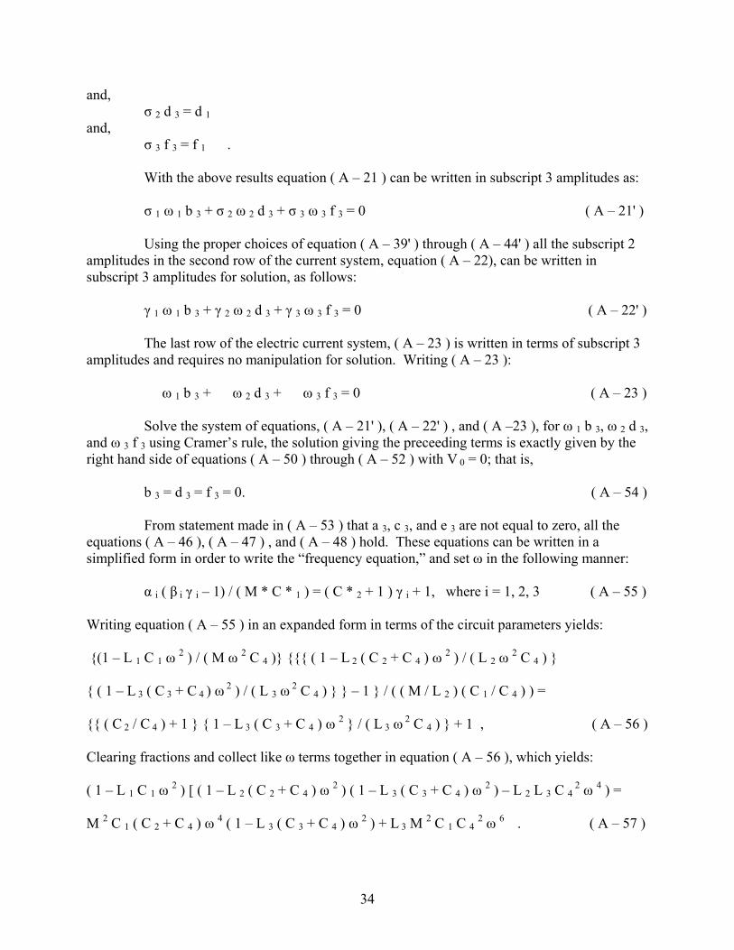
and, σ 2 d 3 = d 1 and, σ 3 f 3 = f 1 . With the above results equation ( A – 21 ) can be written in subscript 3 amplitudes as: σ 1 ω 1 b 3 + σ 2 ω 2 d 3 + σ 3 ω 3 f 3 = 0 ( A – 21' ) Using the proper choices of equation ( A – 39' ) through ( A – 44' ) all the subscript 2 amplitudes in the second row of the current system, equation ( A – 22), can be written in subscript 3 amplitudes for solution, as follows: γ 1 ω 1 b 3 + γ 2 ω 2 d 3 + γ 3 ω 3 f 3 = 0 ( A – 22' ) The last row of the electric current system, ( A – 23 ) is written in terms of subscript 3 amplitudes and requires no manipulation for solution. Writing ( A – 23 ): ω 1 b 3 + ω 2 d 3 + ω 3 f 3 = 0 ( A – 23 ) Solve the system of equations, ( A – 21' ), ( A – 22' ) , and ( A –23 ), for ω 1 b 3, ω 2 d 3, and ω 3 f 3 using Cramer’s rule, the solution giving the preceeding terms is exactly given by the right hand side of equations ( A – 50 ) through ( A – 52 ) with V 0 = 0; that is, b 3 = d 3 = f 3 = 0. ( A – 54 ) From statement made in ( A – 53 ) that a 3, c 3, and e 3 are not equal to zero, all the equations ( A – 46 ), ( A – 47 ) , and ( A – 48 ) hold. These equations can be written in a simplified form in order to write the “frequency equation,” and set ω in the following manner: α i ( β i γ i – 1) / ( M * C * 1 ) = ( C * 2 + 1 ) γ i + 1, where i = 1, 2, 3 ( A – 55 ) Writing equation ( A – 55 ) in an expanded form in terms of the circuit parameters yields: {(1 – L 1 C 1 ω 2 ) / ( M ω 2 C 4 )} {{{ ( 1 – L 2 ( C 2 + C 4 ) ω 2 ) / ( L 2 ω 2 C 4 ) } { ( 1 – L 3 ( C 3 + C 4 ) ω 2 ) / ( L 3 ω 2 C 4 ) } } – 1 } / ( ( M / L 2 ) ( C 1 / C 4 ) ) = {{ ( C 2 / C 4 ) + 1 } { 1 – L 3 ( C 3 + C 4 ) ω 2 } / ( L 3 ω 2 C 4 ) } + 1 , ( A – 56 ) Clearing fractions and collect like ω terms together in equation ( A – 56 ), which yields: ( 1 – L 1 C 1 ω 2 ) [ ( 1 – L 2 ( C 2 + C 4 ) ω 2 ) ( 1 – L 3 ( C 3 + C 4 ) ω 2 ) – L 2 L 3 C 4 2 ω 4 ) = M 2 C 1 ( C 2 + C 4 ) ω 4 ( 1 – L 3 ( C 3 + C 4 ) ω 2 ) + L 3 M 2 C 1 C 4 2 ω 6 . ( A – 57 )

34

Collect terms and write the frequency equation in descending powers of ω yields the cubic equation ( 2 ) in ω 2 of the earlier section III of this paper as: { ( 1 – k 2 ) L 1 L 2 L 3 C 1 [ C 2 C 3 + C 4 ( C 2 + C 3 ) ] } ω 6 – { ( 1 – k 2 ) L 1 L 2 C 1 ( C 2 + C 4 ) L 2 L 3 [ C 2 C 3 + C 4 ( C 2 + C 3 ) ] + L 3 L 1 C 1 ( C 3 + C 4 ) } ω 4 + [ L 1 C 1 + L 2 ( C 2 + C 4 ) + L 3 ( C 3 + C 4 ) ] ω 2 – 1 = 0 . ( 2 ) The three positive roots, ω 1 2, ω 2 2, and ω 3 2 of equation ( 2 ) are the modal or natural angular frequencies of the system. The lower frequency, ω 1 2, is the fundamental natural frequency.

35

REFERENCES 1E. A. Abramyam, “Transformer type accelerators for intense electron beams,” IEEE Trans. Nucl. Sci. 18, p.447, (1970). 2G. J. Rohwein, “A 3 MV transformer for charging pulse lines,” IEEE Trans. Nucl. Sci. 26, p.4211,(1979). 3G. J. Rohwein, “Development of a 3 MV pulse transformer,” Report SAN 79-0813, Sandia Laboratories, (1979). 4Margaret Cheny, and Robert Uth, TESLA, see p.45 and p.87, Barnes and Noble, (1999). 5N. Tesla, Colorado Springs Notes 1899-1900, see p.79, Nolit, Belgrade, Yugoslavia, (1978). 6N. Tesla, U. S. Patent No. 1119732, (1 December 1914). 7V. L. Mangold, (personal communications), 8121 Forest City Rd., Orlando, Florida, 32810. 8ibid. 4, Vernon Mangold, see acknowledgements in front flyleaf. 9K. A. Zheltov, A. V. Malygin, M. G. Plichkin, and V. F. Shalimanov, “Miniature voltage pulse generator for subnanosecond electron accelerators,” Pribory I Tekhnika Eksperimentp, p.90 – 92, (May – June, 1983). 10F. M. Bieniosek, J. Honig, and E. A. Theby, “MEDEA II two-pulse generator development,” Review of Scientific Instruments, 61 (6), p.1713-1716, (June 1990). 11F. M. Bieniosek, “Triple resonance pulse transformer circuit,” Review of Scientific Instruments, 61 (6), p.1717, (June 1990). 12F. M. Bieniosek, Proc. 6th IEEE Pulsed Power Conference, p.700, (1987). 13F. M. Bieniosek, U. S. Patent No. 4833421, (23 May, 1989). 14A. C. M. de Queiroz, “Designing a Tesla magnifier,” Web page at www.coe.ufrj.br/~acmq/magnifier.html. 15P. Drude, Annalen der Physik, (Leipzig) 13, p.512-561, (1904). 16D. Finkelstein, P. Goldberg, and J. Shuchatowitz, “High voltage impulse system,” Review of Scientific Instruments, 37 (2), p.159-162, (February 1966). 17J. L. Reed,”Greater voltage gain for Tesla-transformer accelerators,” Review of Scientific Instruments, 59 (10), p.2300-2301, (October 1988).

36

18R. G. Medhurst, “H. F. resistance and self-capacitance of single-layer solenoids,” Wireless Engineer, p.35-43, (February 1947), and continued in (March 1947), p.80-92. 19F. W. Grover, Inductance Calculations, Dover Publications, New York, (1973). 20Heinrich G. Jacob, “An engineering optimization method with application to STOL-aircraft approach and landing trajectories,” NASA Technical Note D-6978, (1972), Ames Research Center, Moffett Field, CA, 94035. Unrestricted – Publicly Available 21T. von Karman and M. A. Biot, Mathematical Methods in Engineering, see Chapter 6, section 6, McGraw-Hill, New York, (1940). 22Computer code, OrCAD Pspice, OrCAD, 9300 SW Nimbus Ave., Beverton, OR, 97008, Corporate office telephone: (503) 671-9500. 23Computer code, GRAPHIT, Gracces Software Development, 1150 Windmill Ln., Pittsburgh, PA, 15237. 24L. S. Jacobsen, and R. S. Ayre: Engineering Vibrations, see chapters 7 and 8, McGraw-Hill, New York, (1958). 25T. S. E. Thomas, “The capacitance of an anchor ring,” Australian Journal of Physics, 7, p.347, (1954). 26A. C. M. de Queiroz, “Synthesis of multiple resonance networks,” 2000 IEEE ISCAS, Geneva, Switzerland, V, p.413-416, (May 2000). 27N. O. Myklestad, Fundamentals of Vibration Analysis, see Chapter 5,p.154, McGraw-Hill, New York, ( 1956 ). 28J. P. Den Hartog, Mechanical Vibrations, see Chapters 3 and 4, second edition, McGraw-Hill, (1940). 29Computer code, Lahey Computer Systems, Software Solutions for Science & Engineering, Lahey / Fujitsu Fortran LF95 Express v5.7, 865 Tahoe Blvd., Suite 214, Incline Village, Nevada 89450. 30V. G. Welsby and W. G. Radley, The Theory and Design of Inductance Coils, Chapter 7, Macdonald Publishers, London, ( 1950 ). 31G. N. Glasoe and J. V. Lebacqz, Pulse Generators, see pages 184 and 185, Dover Publications, New York, (1965).

37