Embed Size (px)
Citation preview
Designing Parametric Cubic Curves
CS4395: Computer Graphics 1
Mohan SridharanBased on slides created by Edward Angel
Objectives
• Introduce the types of curves:– Interpolating.– Hermite.– Bezier.– B-spline.
• Analyze their performance.
CS4395: Computer Graphics 2
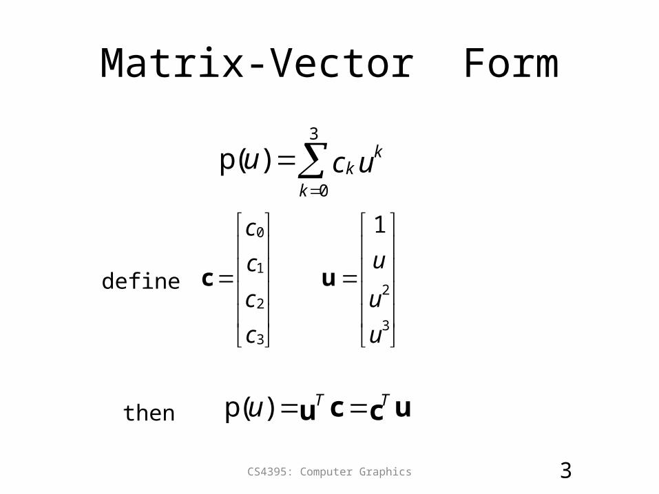
Matrix-Vector Form
CS4395: Computer Graphics 3
ucu k
kk
3
0
)(p
c
c
c
c
3
2
1
0
c
u
u
u
3
2
1
udefine
uccu TTu )(pthen

Interpolating Curve
CS4395: Computer Graphics 4
p0
p1
p2
p3
Given four data (control) points p0 , p1 ,p2 , p3
determine cubic p(u) which passes through them
Must find c0 ,c1 ,c2 , c3
Interpolation Equations
CS4395: Computer Graphics 5
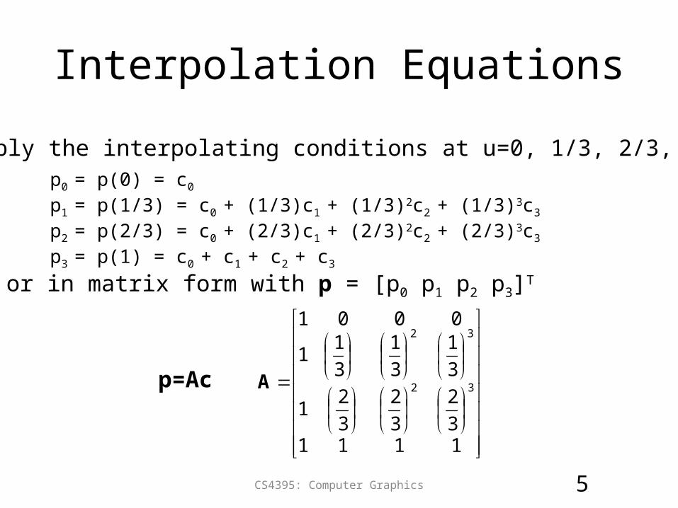
Apply the interpolating conditions at u=0, 1/3, 2/3, 1p0 = p(0) = c0
p1 = p(1/3) = c0 + (1/3)c1 + (1/3)2c2 + (1/3)3c3
p2 = p(2/3) = c0 + (2/3)c1 + (2/3)2c2 + (2/3)3c3
p3 = p(1) = c0 + c1 + c2 + c3
or in matrix form with p = [p0 p1 p2 p3]T
p=Ac
11113
2
3
2
3
21
3
1
3
1
3
11
0001
32
32
A
Interpolation Matrix
CS4395: Computer Graphics 6
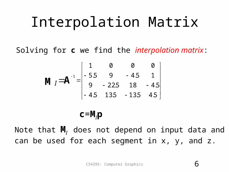
Solving for c we find the interpolation matrix:
5.45.135.135.4
5.4185.229
15.495.5
0001
1
AMI
c=MIp
Note that MI does not depend on input data and
can be used for each segment in x, y, and z.
Interpolating Multiple Segments
CS4395: Computer Graphics 7
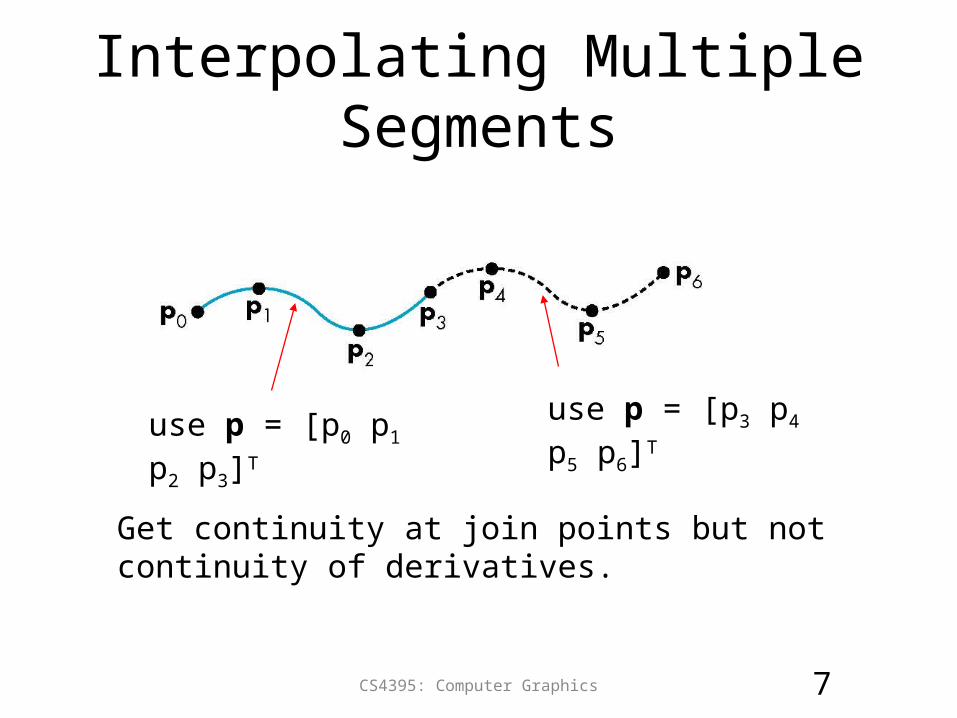
use p = [p0 p1 p2 p3]T use p = [p3 p4 p5 p6]T
Get continuity at join points but not continuity of derivatives.
Blending Functions
CS4395: Computer Graphics 8
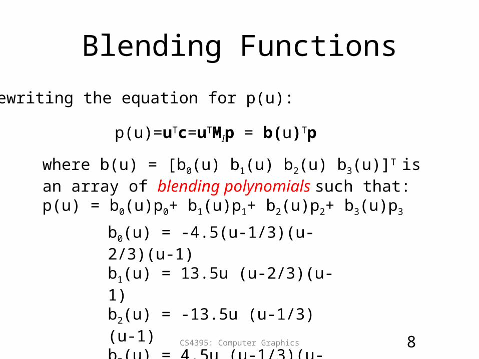
Rewriting the equation for p(u):
p(u)=uTc=uTMIp = b(u)Tp
where b(u) = [b0(u) b1(u) b2(u) b3(u)]T is an array of blending polynomials such that:p(u) = b0(u)p0+ b1(u)p1+ b2(u)p2+ b3(u)p3
b0(u) = -4.5(u-1/3)(u-2/3)(u-1)b1(u) = 13.5u (u-2/3)(u-1)b2(u) = -13.5u (u-1/3)(u-1)b3(u) = 4.5u (u-1/3)(u-2/3)
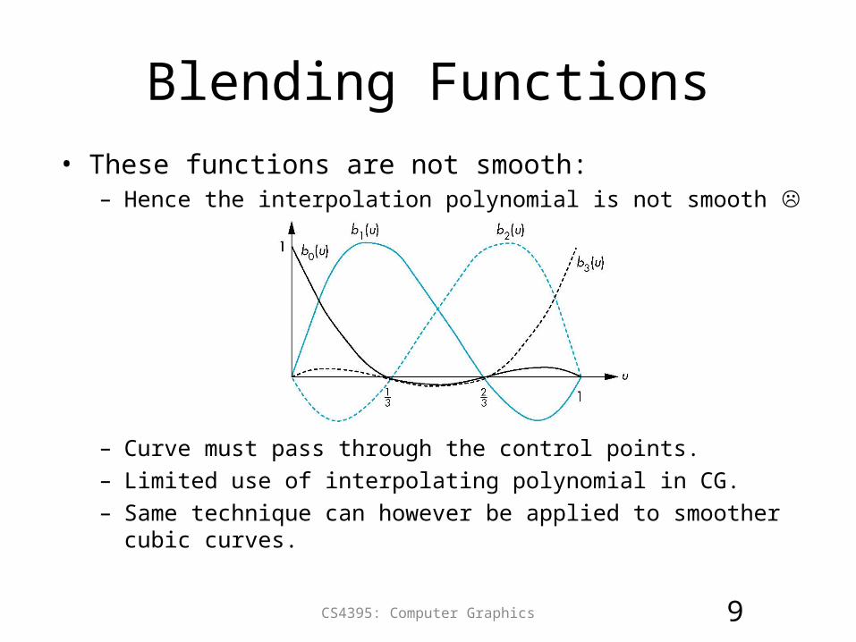
Blending Functions• These functions are not smooth:
– Hence the interpolation polynomial is not smooth
– Curve must pass through the control points.– Limited use of interpolating polynomial in CG.– Same technique can however be applied to smoother cubic curves.
CS4395: Computer Graphics 9
Interpolating Patch
CS4395: Computer Graphics 10
vucvup j
jij
i
oi
3
0
3
),(
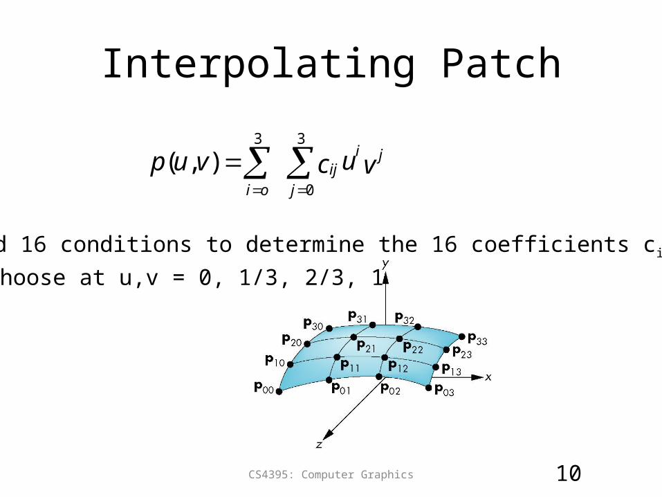
Need 16 conditions to determine the 16 coefficients cij
Choose at u,v = 0, 1/3, 2/3, 1
Matrix Form
CS4395: Computer Graphics 11
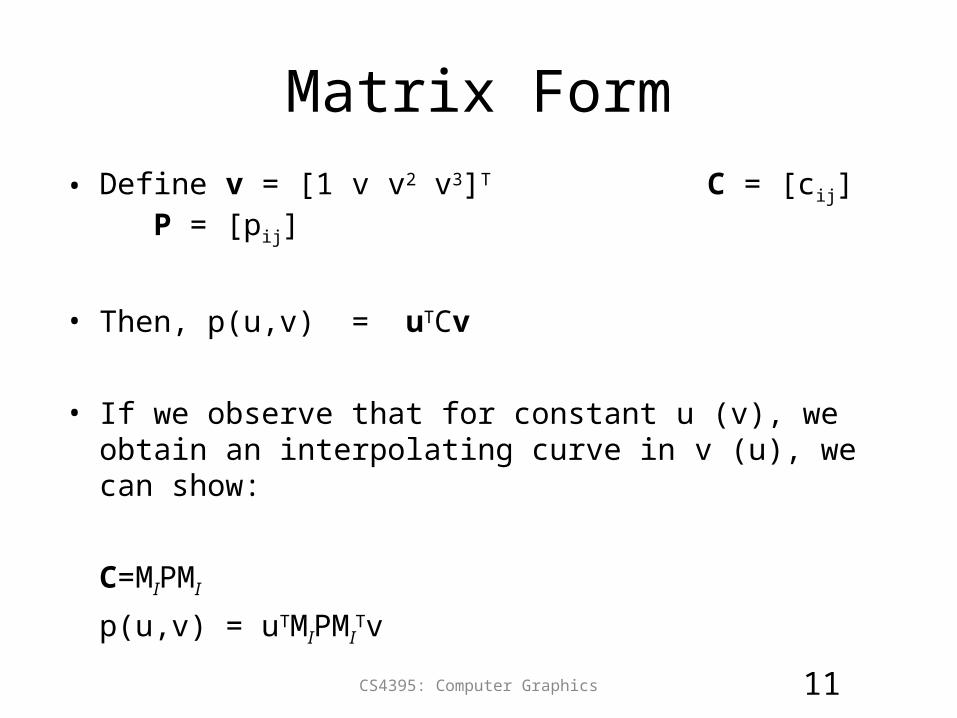
• Define v = [1 v v2 v3]T C = [cij] P = [pij]
• Then, p(u,v) = uTCv
• If we observe that for constant u (v), we obtain an interpolating curve in v (u), we can show:
C=MIPMI
p(u,v) = uTMIPMITv
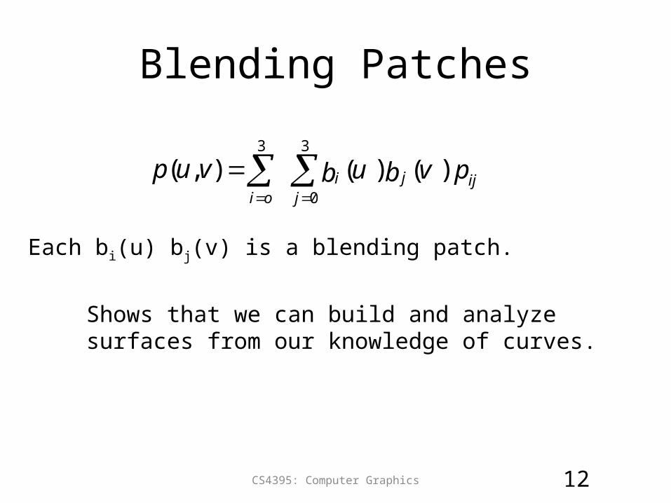
Blending Patches
CS4395: Computer Graphics 12
pvbubvup ijjj
ioi
)()(),(3
0
3
Each bi(u) bj(v) is a blending patch.
Shows that we can build and analyze surfaces from our knowledge of curves.
Other Types of Curves and Surfaces
• Need to overcome limitations of interpolating form:– Lack of smoothness.– Discontinuous derivatives at join points.
• Four conditions (for cubics) that can be applied to each segment:– Use them other than for interpolation.– Need only come close to the data.
CS4395: Computer Graphics 13
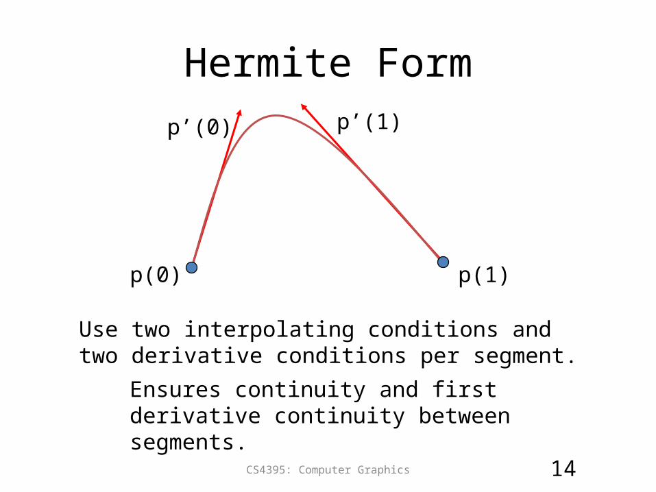
Hermite Form
CS4395: Computer Graphics 14
p(0) p(1)
p’(0) p’(1)
Use two interpolating conditions and two derivative conditions per segment.
Ensures continuity and first derivative continuity between segments.
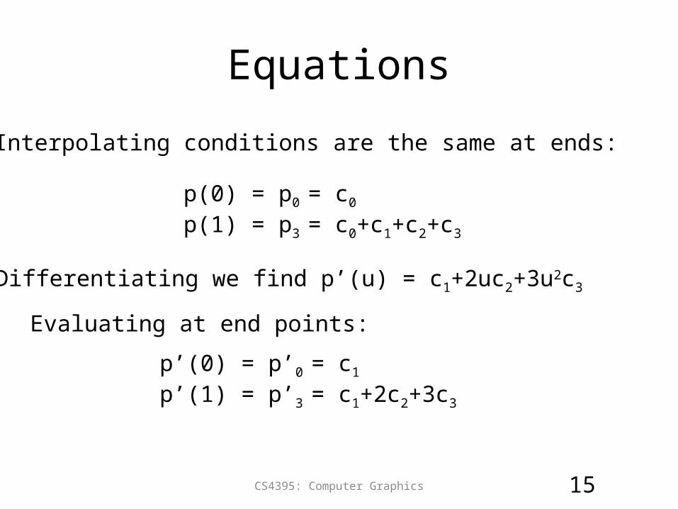
Equations
CS4395: Computer Graphics 15
Interpolating conditions are the same at ends:
p(0) = p0 = c0
p(1) = p3 = c0+c1+c2+c3
Differentiating we find p’(u) = c1+2uc2+3u2c3
Evaluating at end points:
p’(0) = p’0 = c1
p’(1) = p’3 = c1+2c2+3c3
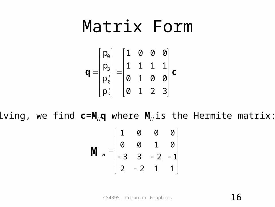
Matrix Form
CS4395: Computer Graphics 16
cq
3210
0010
1111
0001
p'
p'
p
p
3
0
3
0
Solving, we find c=MHq where MH is the Hermite matrix:
1122
1233
0100
0001
MH
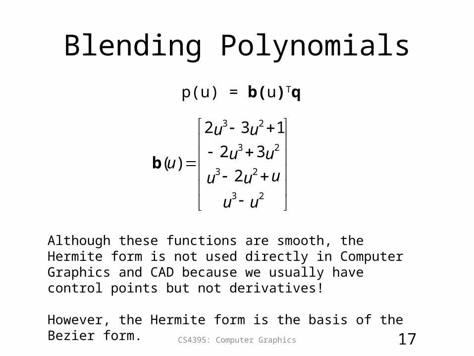
Blending Polynomials
CS4395: Computer Graphics 17
p(u) = b(u)Tq
uu
uuu
uu
uu
u
23
23
23
23
2
32
132
)(b
Although these functions are smooth, the Hermite form is not used directly in Computer Graphics and CAD because we usually have control points but not derivatives!
However, the Hermite form is the basis of the Bezier form.
Parametric and Geometric Continuity
• We can require the parameters and the derivatives to be continuous at join points (parametric continuity).
• Alternately, we can require that the tangents of the resulting curve be continuous (geometry continuity).– Derivative at a point on a curve defines a tangent line.– Require that the derivatives be proportional.
• The latter gives more flexibility as we need to satisfy only two conditions rather than three at each join point.
CS4395: Computer Graphics 18
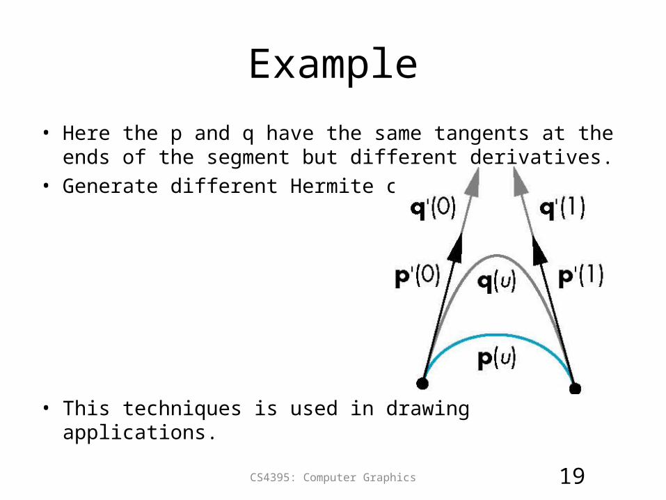
Example
• Here the p and q have the same tangents at the ends of the segment but different derivatives.
• Generate different Hermite curves.
• This techniques is used in drawing applications.
CS4395: Computer Graphics 19
Higher Dimensional Approximations
• The techniques for both interpolating and Hermite curves can be used with higher dimensional parametric polynomials.
• For interpolating form, the matrix becomes increasingly more ill-conditioned and the resulting curves less smooth and more prone to numerical errors.
• In both cases, there is considerable work in rendering the resulting polynomial curves and surfaces.
CS4395: Computer Graphics 20