Chapter 3: Geometric Objects and Transformations Part 2 E. Angel and D. Shreiner: Interactive Computer Graphics 6E © Addison-Wesley 2012 1 Mohan Sridharan

Chapter 3: Geometric Objects and Transformations

Part 2

E. Angel and D. Shreiner: Interactive Computer Graphics 6E © Addison-Wesley

20121

Mohan SridharanBased on Slides by Edward Angel and Dave Shreiner

Objectives

• Introduce standard transformations:– Rotation.– Translation.– Scaling.– Shear.

• Derive homogeneous coordinate transformation matrices.

• Learn to build arbitrary transformation matrices from simple transformations.


20122

General Transformations

A transformation maps points to other points and/or vectors to other vectors:


20123

Q=T(P)

v=T(u)

Affine Transformations

• Line preserving.

• Characteristic of many physically important transformations!– Rigid body transformations: rotation, translation.– Scaling, shear.

• Important in graphics since we need only transform endpoints of line segments and let implementation draw line segment between the transformed endpoints!


20124

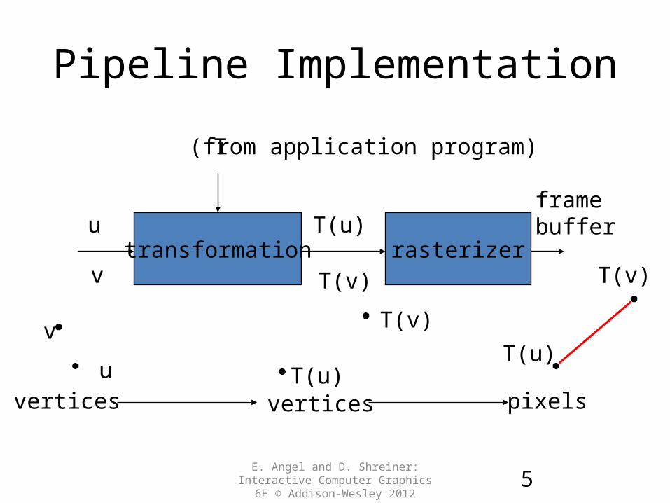
Pipeline Implementation

v


20125

transformation rasterizer

u

u

v

T

T(u)

T(v)

T(u)T(u)

T(v)

T(v)

vertices vertices pixels

framebuffer

(from application program)

Notation• We will be working with both coordinate-free representations

of transformations and representations within a frame: P,Q, R: points in an affine space.

u, v, w: vectors in an affine space. , , : scalars.

• p, q, r: representations of points

array of 4 scalars in homogeneous coordinates.

• u, v, w: representations of pointsarray of 4 scalars in homogeneous coordinates.


20126

Translation• Move (translate, displace) a point to a new location.

• Displacement determined by a vector d:– Three degrees of freedom.– P’=P+d


20127

P

P’

d

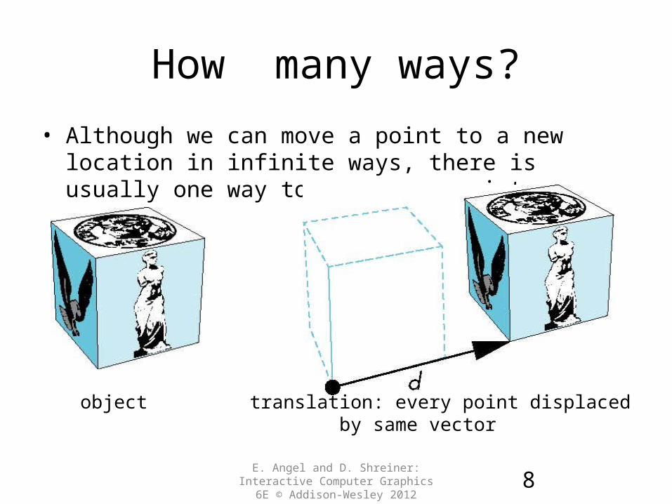
How many ways?

• Although we can move a point to a new location in infinite ways, there is usually one way to move many points.


20128

object translation: every point displaced by same vector

Translation Using Representations

• Using the homogeneous coordinate representation in some frame:

p=[ x y z 1]T

p’=[x’ y’ z’ 1]T

d=[dx dy dz 0]T

• Hence p’ = p + d or: x’=x+dx

y’=y+dy

z’=z+dz


20129

note that this expression is in four dimensions and expressespoint = vector + point

Translation Matrix• We can also express translation using a 4 x 4 matrix T in homogeneous

coordinates p’=Tp where:

T = T(dx, dy, dz) =

• This form is better for implementation because all affine transformations can be expressed this way and multiple transformations can be concatenated together


201210

1000

d100

d010

d001

z

y

x

Rotation (2D)

• Consider rotation about the origin by degrees:– radius stays the same, angle increases by


201211

x’=x cos –y sin y’ = x sin + y cos

x = r cos y = r sin

x = r cos (y = r sin (

Rotation about the z axis

• Rotation about z axis in three dimensions leaves all points with the same z.– Equivalent to rotation in two dimensions in planes of constant z

– or in homogeneous coordinates p’=Rz()p


201212

x’=x cos –y sin y’ = x sin + y cos z’ =z

Rotation Matrix

R = Rz() =


201213

1000

0100

00 cossin

00sin cos

Rotation about x and y axes

• Same argument as for rotation about z axis:– For rotation about x axis, x is unchanged.– For rotation about y axis, y is unchanged.


201214

R = Rx() =

R = Ry() =

1000

0 cos sin0

0 sin- cos0

0001

1000

0 cos0 sin-

0010

0 sin0 cos

Scaling

S = S(sx, sy, sz) =


201215

1000

000

000

000

z

y

x

s

s

s

x’=sxxy’=syxz’=szx

p’=Sp

Expand or contract along each axis (fixed point of origin)

Reflection

Reflection corresponds to negative scale factors:


201216

Originalsx = -1 sy = 1

sx = -1 sy = -1 sx = 1 sy = -1

Shear

• Helpful to add one more basic transformation.

• Equivalent to pulling faces in opposite directions


201217

Shear Matrix

Consider simple shear along x axis:


201218

x’ = x + y cot y’ = yz’ = z

1000

0100

0010

00cot 1

H() =

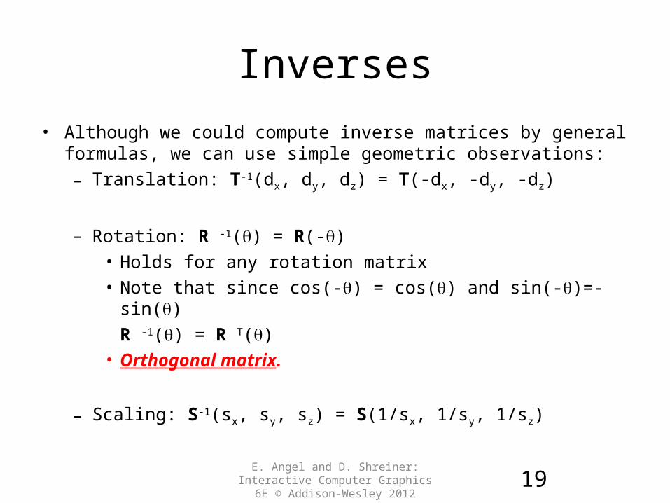
Inverses• Although we could compute inverse matrices by general formulas, we can

use simple geometric observations:– Translation: T-1(dx, dy, dz) = T(-dx, -dy, -dz)

– Rotation: R -1() = R(-)

• Holds for any rotation matrix

• Note that since cos(-) = cos() and sin(-)=-sin()

R -1() = R T()

• Orthogonal matrix.

– Scaling: S-1(sx, sy, sz) = S(1/sx, 1/sy, 1/sz)


201219

Concatenation• We can form arbitrary affine transformation matrices by multiplying

together rotation, translation, and scaling matrices.

• Because the same transformation is applied to many vertices, the cost of forming a matrix M=ABCD is not significant compared to the cost of computing Mp for many vertices p.

• The difficult part is how to form a desired transformation from the specifications in the application.


201220

Order of Transformations

• Note that matrix on the right is the first applied.

• Mathematically, the following are equivalent: p’ = ABCp = A(B(Cp))

• Note many references use column matrices to represent points. In terms of column matrices:

p’T = pTCTBTAT


201221

General Rotation About the Origin


201222

A rotation by about an arbitrary axis can be decomposed into the concatenation of rotations about the x, y, and z axes

R() = Rz(z) Ry(y) Rx(x)

x y z are called the Euler angles

Rotations do not commute. We can use rotations in another order but with different angles.

x

z

yv

Rotation About a Fixed Point other than the Origin

1. Move fixed point to origin.2. Rotate.3. Move fixed point back.

M = T(pf) R() T(-pf)


201223

Instancing• In modeling, we often start with a simple object prototypes centered at

the origin, oriented with the axis, and at a standard size.

• Obtain desired instances of the object using an affine transformation.

• Apply an instance transformation to vertices to:Scale , Orient, Locate!

• Load object prototype in server.

• Send appropriate instance transform.


201224

25E. Angel and D. Shreiner: Interactive

Computer Graphics 6E © Addison-Wesley 2012

Objectives

• Learn how to carry out transformations in OpenGL:– Rotation.– Translation .– Scaling.

• Introduce <mat.h> and <vec.h> transformations:– Model-view.– Projection.



Pre 3.1OpenGL Matrices• In OpenGL matrices were part of the state.

• Multiple types:– Model-View (GL_MODELVIEW).– Projection (GL_PROJECTION).– Texture (GL_TEXTURE).– Color(GL_COLOR).

• Single set of functions for manipulation!

• Select which to manipulated by:– glMatrixMode(GL_MODELVIEW);– glMatrixMode(GL_PROJECTION);



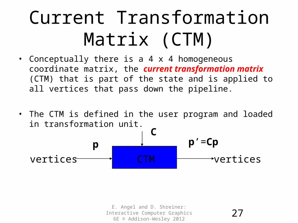
Current Transformation Matrix (CTM)

• Conceptually there is a 4 x 4 homogeneous coordinate matrix, the current transformation matrix (CTM) that is part of the state and is applied to all vertices that pass down the pipeline.

• The CTM is defined in the user program and loaded in transformation unit.

CTMvertices vertices

p p’=CpC



CTM Operations• The CTM can be altered by loading a new CTM or by post-multiplication:

Load an identity matrix: C ILoad an arbitrary matrix: C M

Load a translation matrix: C TLoad a rotation matrix: C RLoad a scaling matrix: C S

Post-multiply by an arbitrary matrix: C CMPost-multiply by a translation matrix: C CTPost-multiply by a rotation matrix: C C RPost-multiply by a scaling matrix: C C S



Rotation about a Fixed Point

1. Start with identity matrix: C I

2. Move fixed point to origin: C CT i.e., CT(-pf)

3. Rotate: C CR i.e., CR()

4. Move fixed point back: C CT -1 i.e., CT(pf)

Result: C = TR T –1 i.e., T(-pf) R() T(pf) which is backwards!We want: M = T(pf) R() T(-pf)

This result is a consequence of doing postmultiplications. Let us try again!



Reversing the Order

We want C = T –1 R T i.e., T(pf) R() T(-pf)so we must do the operations in the following (reverse) order:

C IC CT -1

C CRC CT

Each operation corresponds to one function call in the program.

The last operation specified is the first executed in the program

See Section 3.11.3 and Section 3.11.4.



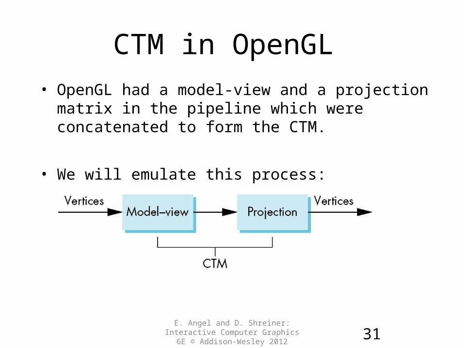
CTM in OpenGL • OpenGL had a model-view and a projection matrix in the

pipeline which were concatenated to form the CTM.

• We will emulate this process:



Rotation, Translation, Scaling

Create an identity matrix: mat4 m = Identity();

Multiply on right by rotation matrix of theta in degrees where (vx, vy, vz) define axis of rotation:mat4 r = Rotate(theta, vx, vy, vz)m = m*r;

Do same with translation and scaling:mat4 s = Scale( sx, sy, sz)mat4 t = Translate(dx, dy, dz);m = m*s*t;



Example

• Rotation about z axis by 30 degrees with a fixed point of (1.0, 2.0, 3.0):

• Remember that last matrix specified is the first applied!

• You can write your own versions of <Translate> and <Rotate>.• Functions defined in <angel.h> – you at your own risk

mat 4 m = Identity();m = Translate(1.0, 2.0, 3.0)* Rotate(30.0, 0.0, 0.0, 1.0)* Translate(-1.0, -2.0, -3.0);



Arbitrary Matrices

• Can load and multiply by matrices defined in the application program.

• Matrices are stored as one dimensional array of 16 elements which are the components of the desired 4 x 4 matrix stored by columns

• OpenGL functions that have matrices as parameters allow the application to send the matrix or its transpose.



Matrix Stacks

• In many situations we want to save transformation matrices for later use:– Traversing hierarchical data structures (Chapter 8).– Avoiding state changes when executing display lists.

• Pre 3.1 OpenGL maintained stacks for each type of matrix.

• Easy to create the same functionality with a simple stack class.



Reading Back State

• Can also access OpenGL variables (and other parts of the state) by query functions

• Why do we need these query functions?

glGetIntegervglGetFloatvglGetBooleanvglGetDoublevglIsEnabled



Using Transformations

• Example: use idle function to rotate a cube and mouse function to change direction of rotation.

• Start with a program that draws a cube in a standard way– Centered at origin.– Sides aligned with axes.– Will discuss modeling shortly.



main.c void main(int argc, char **argv) { glutInit(&argc, argv); glutInitDisplayMode(GLUT_DOUBLE | GLUT_RGB | GLUT_DEPTH); glutInitWindowSize(500, 500); glutCreateWindow("colorcube"); glutReshapeFunc(myReshape); glutDisplayFunc(display); glutIdleFunc(spinCube); glutMouseFunc(mouse); glEnable(GL_DEPTH_TEST); glutMainLoop();}



Idle and Mouse callbacksvoid spinCube() {

theta[axis] += 2.0;if( theta[axis] > 360.0 ) theta[axis] -= 360.0;glutPostRedisplay();

}

void mouse(int btn, int state, int x, int y)

{

if(btn==GLUT_LEFT_BUTTON && state == GLUT_DOWN)

axis = 0;

if(btn==GLUT_MIDDLE_BUTTON && state == GLUT_DOWN)

axis = 1;

if(btn==GLUT_RIGHT_BUTTON && state == GLUT_DOWN)

axis = 2;

}



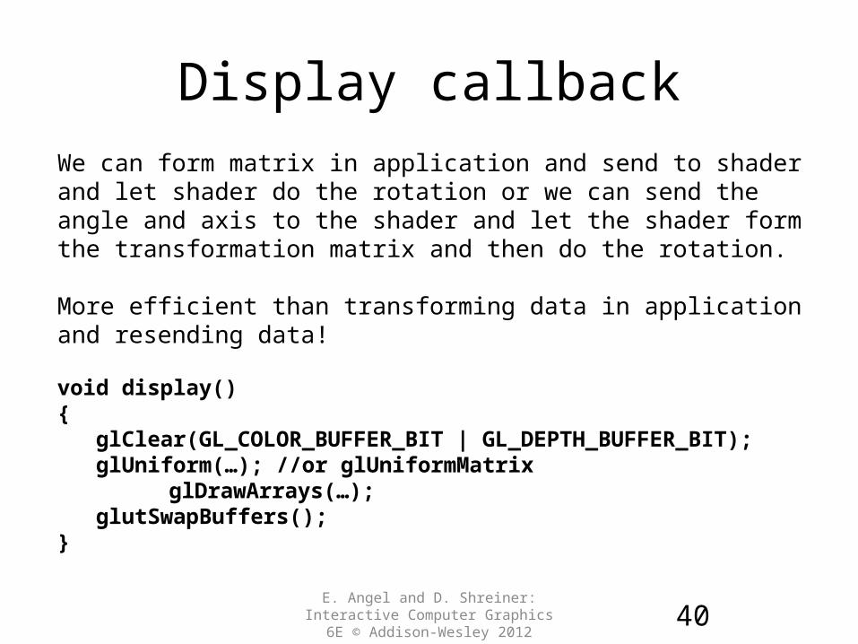
Display callbackWe can form matrix in application and send to shader and let shader do the rotation or we can send the angle and axis to the shader and let the shader form the transformation matrix and then do the rotation.

More efficient than transforming data in application and resending data!

void display(){ glClear(GL_COLOR_BUFFER_BIT | GL_DEPTH_BUFFER_BIT); glUniform(…); //or glUniformMatrix

glDrawArrays(…); glutSwapBuffers();}



Using the Model-view Matrix

• In OpenGL the model-view matrix is used to:– Position the camera: can be done by rotations and translations but

often easier to use a <LookAt> function.– Build models of objects.

• The projection matrix is used to define the view volume and to select a camera lens.

• Although these matrices are no longer part of the OpenGL state, it is a good strategy to create them in our applications.



Smooth Rotation

• From a practical standpoint, we are often want to use transformations to move and reorient an object smoothly:– Problem: find a sequence of model-view matrices M0,M1,…..,Mn so

that when they are applied successively to one or more objects we see a smooth transition!

• For orientating an object, we can use the fact that every rotation corresponds to part of a great circle on a sphere:– Find the axis of rotation and angle.– Virtual trackball (see Section 3.13.2).



Incremental Rotation

• Consider the two approaches:– For a sequence of rotation matrices R0,R1,…..,Rn , find the Euler

angles for each and use Ri= Riz Riy Rix

• Not very efficient – Use the final positions to determine the axis and angle of rotation,

then increment only the angle.

• Quaternions can be more efficient than either



Quaternions• Extension of imaginary numbers from 2D to 3D.

• Requires one real and three imaginary components: i, j, k

• Quaternions can express rotations on sphere smoothly and efficiently. Process:– Model-view matrix quaternion– Carry out operations with quaternions– Quaternion Model-view matrix

• See Section 3.14.

q=q0+q1i+q2j+q3k



Interfaces

• One of the major problems in interactive computer graphics is how to use 2D devices such as a mouse to interface with 3D objects.

• Example: how to form an instance matrix?

• Some alternatives:– Virtual trackball.– 3D input devices such as the space-ball.– Use areas of the screen: distance from center controls angle, position,

scale depending on mouse button depressed.

What Next?

• An overview of model generation.

• Move on to viewing and projections.

• Be prepared for programming project-2.


201246

Documents

Chapter 3: Geometric Objects and Transformations Part 2 E. Angel and D. Shreiner: Interactive Computer Graphics 6E © Addison-Wesley 2012 1 Mohan Sridharan