Designing a cluster for geophysical fluid dynamics applications

Designing a cluster for geophysical fluid dynamics

applications

Göran BroströmDep. of Oceanography, Earth Science

Centre, Göteborg University.

Our cluster(me and Johan Nilsson, Dep. of Meterology,

Stockholm University)

• Grant from the Knut & Alice Wallenberg foundation (1.4 MSEK)

• 48 cpu cluster• Intel P4 2.26 Ghz• 500 Mb 800Mhz Rdram• SCI cards

• Delivered by South Pole• Run by NSC (thanks Niclas & Peter)

What we study

Geophysical fluid dynamics

• Oceanography

• Meteorology

• Climate dynamics

Thin fluid layersLarge aspect ratio

Highly turbulentGulf stream: Re~1012

Large variety of scales

Parameterizations are important in geophysical fluid dynamics

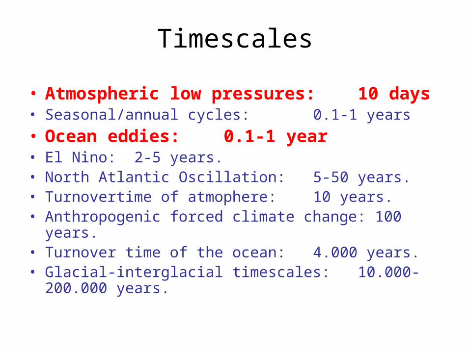
Timescales

• Atmospheric low pressures: 10 days

• Seasonal/annual cycles: 0.1-1 years

• Ocean eddies: 0.1-1 year• El Nino: 2-5 years.• North Atlantic Oscillation: 5-50 years.• Turnovertime of atmophere: 10 years.• Anthropogenic forced climate change: 100 years.• Turnover time of the ocean: 4.000 years.• Glacial-interglacial timescales: 10.000-200.000 years.

Some examples of atmospheric and oceanic low pressures.

Timescales

• Atmospheric low pressures: 10 days• Seasonal/annual cycles: 0.1-1 years• Ocean eddies: 0.1-1 year

• El Nino: 2-5 years.• North Atlantic Oscillation: 5-50 years.• Turnovertime of atmophere: 10 years.• Anthropogenic forced climate change: 100 years.• Turnover time of the ocean: 4.000 years.• Glacial-interglacial timescales: 10.000-200.000 years.

Normal state

Initial ENSO state

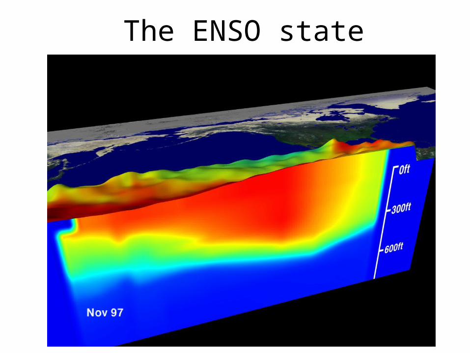
The ENSO state

The ENSO state

Timescales

• Atmospheric low pressures: 10 days• Seasonal/annual cycles: 0.1-1 years• Ocean eddies: 0.1-1 year• El Nino: 2-5 years.

• North Atlantic Oscillation: 5-50 years.• Turnovertime of atmophere: 10 years.• Anthropogenic forced climate change: 100 years.• Turnover time of the ocean: 4.000 years.• Glacial-interglacial timescales: 10.000-200.000 years.

Positive NAO phase Negative NAO phase

Positive NAO phase Negative NAO phase

Timescales

• Atmospheric low pressures: 10 days• Seasonal/annual cycles: 0.1-1 years• Ocean eddies: 0.1-1 year• El Nino: 2-5 years.• North Atlantic Oscillation: 5-50 years.• Turnovertime of atmophere: 10 years.• Anthropogenic forced climate change: 100 years.

• Turnover time of the ocean: 4.000 years.

• Glacial-interglacial timescales: 10.000-200.000 years.

Temperature in the North Atlantic

Timescales

• Atmospheric low pressures: 10 days• Seasonal/annual cycles: 0.1-1 years• Ocean eddies: 0.1-1 year• El Nino: 2-5 years.

• North Atlantic Oscillation: 5-50 years.• Turnovertime of atmophere: 10 years.• Anthropogenic forced climate change: 100 years.• Turnover time of the ocean: 4.000 years.

• Glacial-interglacial timescales: 10.000-200.000 years.

Ice coverage, sea level

What model will we use?

MIT General circulation model


• General fluid dynamics solver• Atmospheric and ocean physics• Sophisticated mixing schemes• Biogeochemical modules• Efficient solvers• Sophisticated coordinate system• Automatic adjoint schemes• Data assimilation routines

• Finite difference scheme• F77 code• Portable


Spherical coordinates “Cubed sphere”


• General fluid dynamics solver• Atmospheric and ocean physics• Sophisticated mixing schemes• Biogeochemical modules• Efficient solvers• Sophisticated coordinate system• Automatic adjoint schemes• Data assimilation routines

• Finite difference scheme• F77 code• Portable









Some computational aspects

Some tests in INGVAR

(32 AMD 900 Mhz cluster)

Experiments with 60*60*20 grid points




MM5 Regional atmospheric model



Choosing cpu’s, motherboard, memory,

connections

Specfp (swim)

0100200300400500600700

Ru

n t

ime

Run time on different nodes

02000400060008000

1000012000140001600018000

run

tim

e

Choosing interconnection

(requires a cluster to test)

Based on earlier experience we use SCI from Dolphinics (SCALI)

Our choice

• Named Otto• SCI cards• P4 2.26 GHz (single cpus)• 800 Mhz Rdram (500 Mb)• Intel motherboards (the only available)

• 48 nodes• NSC (nicely in the shadow of Monolith)

Otto (P4 2.26 GHz)

Scaling

Otto (P4 2.26 GHz) Ingvar (AMD 900 MHz)

Why do we get this kind of results?

Time spent on different “subroutines”

60*60*20 120*120*20

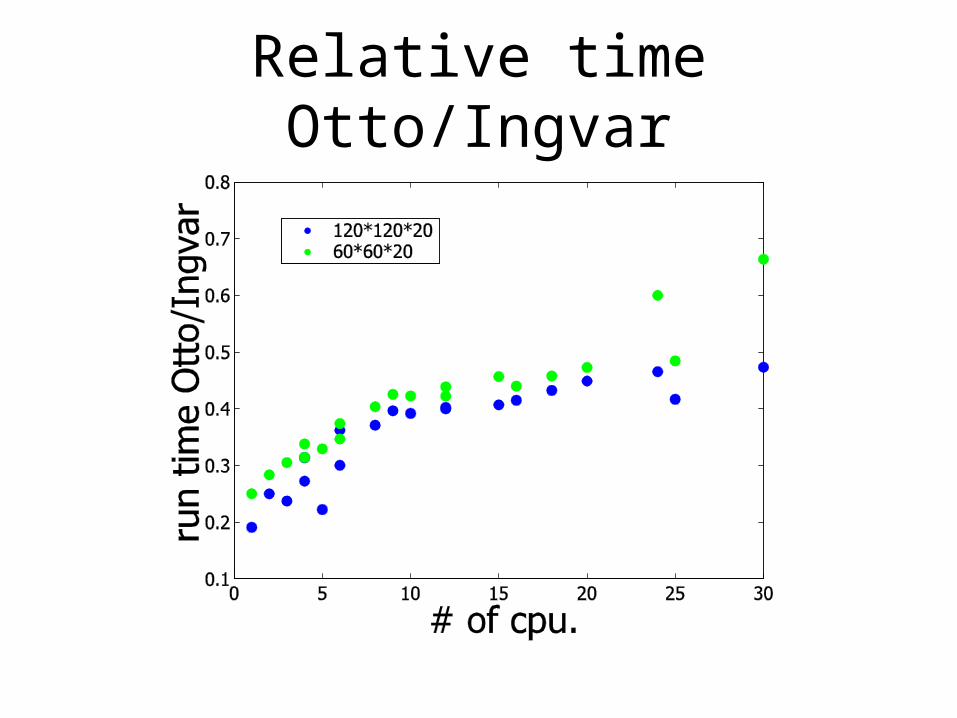
Relative time Otto/Ingvar

Some tests on other machines

• INGVAR: 32 node, AMD 900 MHz, SCI• Idefix: 16 node, Dual PIII 1000 MHz, SCI• SGI 3800: 96 Proc. 500 MHz• Otto: 48 node, P4 2.26 Mhz, SCI• ? MIT, LCS: 32 node, P4 2.26 Mhz, MYRINET

Comparing different system (120*120*20 gridpoints)



SCI or Myrinet?

120*120*20 gridpoints

SCI or Myrinet?

120*120*20 gridpoints (60*60*20 gripoints)

(ooops, I used the ifcCompiler for these tests)

SCI or Myrinet?



(1066Mhz rdram?)

SCI or Myrinet?(time spent in pressure calc.)



(1066Mhz rdram?)

Conclusions

• Linux clusters are useful in computational geophysical fluid dynamics!!

• SCI cards are necessary for parallel runs >10 nodes.• For efficient parallelization: >50*50*20 grid points per

node!• Few users - great for development.

• Memory limitations, for 48 proc. a’ 500 Mb, 1200*1200*30 grid points is maximum (eddy resolving North Atlantic, Baltic Sea).

• For applications similar as ours, go for SCI cards + cpu with fast memory bus and fast memory!!

Experiment with low resolution (eddies are parameterized)

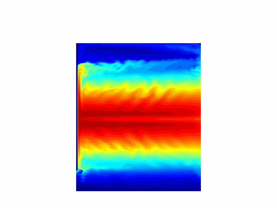
Experiment with low resolution (eddies are parameterized)

Thanks for your attention

Documents

Designing a cluster for geophysical fluid dynamics applications