Embed Size (px)
Citation preview

Journal of International Conference on Electrical Machines and Systems Vol. 1, No.3 , pp. 303 ~ 311 , 2012 303
Design Space Methodology and Its Application in Interior Permanent
Magnet Motor Design
Fan Tao*, Li Qi**, Wen Xuhui* and Xu Longya***
Abstract – An innovative interpretation of the per-unit interior permanent magnet (IPM)
machine model known as Design Space is presented in this paper. Based on the proposed
Design Space formulation, an effective computation method to predict IPM machine
performance factors, such as the current and power factor in a full range of speeds, is
proposed. A systematic methodology is summarized, which translates the full speed range
machine design procedure into the region determination on the so-called Design Space. The
effect of dc-link voltage is also analyzed in a similar manner with the current and power
factor. A series of IPM motors have been designed, and a preferred motor is selected with the
help of the proposed Design Space Methodology (DSM), which has the best tradeoff between
the nominal voltage and the dropped voltage condition. Experiment results show that the
selected motor satisfies the machine requirements and all the design constrains, such as the
current and back-EMF limitations.
Keywords: Design Space, IPM machine, Motor Design, FEA
1. Introduction
The usage of interior permanent magnet motors (IPM) in
traction application is increasing constantly in spite of the
recent uncertainty regarding the availability of the raw
material used for making RE permanent magnets. The most
important reason for that may be the superior performance
with IPM machines, such as excellent field-weakening
capability, high efficiency and the supplemented reluctance
torque.
However, the unchangeable excitation of permanent
magnets makes the IPM machine parameter selection a
challenging job. Excellent work has been done towards to
the parameter selection of SPM type machines [1]. This
paper firstly covers the optimal selection of the key surface
PM machine equivalent circuit parameters using a novel
parameter plane approach. This parameter plane is used to
show how the performance requirements constrain the
allowable machine design. There is also some work looking
at the optimal selection of PM machine parameters for
field-weakening performance [2]-[4], and it shows that
ideally the characteristic current should be equal to the
rated current. Excellent work have been done regarding to
this topic [5]-[8] for IPM machines. Nevertheless, methods
proposed in literature are more or less complex with regards
to aiding the parameter selection procedure. An experienced
designer is still needed to obtain appropriate key machine
parameters. Some other procedures proposed previously are
straight forward, but can only handle the parameter
selection for a single working point. A method with the
capability for parameter selection with respect to the full
speed range and is compute effectively computed has
hardly been seen before now.
An innovative interpretation of the per-unit IPM machine
model is given in the paper, which is named as the Design
Space. Based on the proposed Design Space formulation, a
computation effective method to predict the IPM machine
performance such as current and power factor in the full-
speed range is given. A systematic methodology is
summarized, which translate the full speed range machine
design procedure into the region determination on the so-
called Design Space. The effect of dc-link voltage variation
of the machine performance is considered to some extent.
The requirements and constrains of the IPM motor in a
typical traction application are summarized firstly, which
forms the boundary of the final parameter region. The
Design Space Methodology (DSM) is built-up from the
third section. The formulas in DSM are derived, and key
concepts such as unity design space and general design
space is given in this section. The effect of dc-link voltage
is presented as well.
* Institute of Electrical Engineering of Chinese Academic of Science,
Key Laboratory of Power Electronics Drive, Beijing, P.R.China
** Graduate University of Chinese Academy of Science P.R.China, Be
ijing, P.R.China ([email protected])
*** The Ohio State University Columbus, OH 43210, USA
Received 07 March; Accepted 9 August

304 Design Space Methodology and Its Application in Interior Permanent Magnet Motor Design
In the fourth section, a systematic procedure is given
with the help of the formulas in DSM, which is used to
determine the proper sets of parameter to fulfill the
requirements and constrains described in section II.
In the fifth section, a series of IPM motors have been
designed, and a preferred motor is selected with the help of
the proposed DSM, which has the best tradeoff between the
nominal voltage and the dropped voltage condition.
Experiment results show that, the selected motor satisfy the
machine requirements and all the design constrains, such as
the current and back-EMF limitations.
2. Requirements and Constrains of a Typical Tracti
on Application
An IPM motor used in traction applications will face
quite different requirements and constraints from those of
pumps and fans. A typical curve demonstrates this as
Freedom CAR target of US DOE [9] as shown in Fig.1.
Fig. 1. FreedomCAR traction motor power requirement in a
speed range
There are some key points in the curve. The first is the
corner speed, which is defined as the threshold speed from
where the power requirement keeps constant. The second
one is the maximum speed. The ratio of the two speeds is
called the constant power speed range (CPSR). A typical
CPSR in a traction application is larger than 3~4. The third
point is the peak power point, where peak torque is needed
for a very short duration.
Dou to the great portion of the inverter cost in a traction
system, the current and voltage rating of the power module
in an inverter is strictly constrained. As a result, a certain
current limit is imposed to the accompanying motor. A
typical value of it is 2~3 times that of the natural current at
peak power.
According to previous research [10], the back-EMF at
the maximum speed must be limited to a certain value in
consideration of safety issues related to inverter failure.
The power versus speed requirement and all the design c
onstrains described previously are summarized in Table I, w
hich is a fixture of the US DOE target and the domestic req
uirement.
Table 1. Requirements and Constrains in Traction Motor
Item Value Item Value
Continuous
power 30kW
Peak
torque 200Nm
Corner
speed 2500rpm
Nominal
dc-link
voltage
320VDC
Maximum
speed 7000rpm
dc-
voltage
variation
range
280~360VDC
Peak
power 50kW
Current
limit 270Arms
Rated
efficiency 95%
Line to
line
back-
emf
limit
800Vpk@7000rpm
3. Design Space Methodology
In this section, the DSM is built-up from ground,
beginning with a new interpretation of the per-unit IPM
machine model. The introduction of the per-unit system
brings two beneficial aspects. The first one is making the
resulting formulation in a general manner. What’s more
important, the effect of working point switching can be
seen equivalent to parameter variation.
3.1 Per-unit IPM model
A traditional dq-axis model of the IPM machine is listed
in (1) to (4). ξ is the saliency ratio. ωe is the angular speed
measured in electrical degree. p is pole number of the motor.
Other quantities are self-explainary.
d e m d du l i (1)
q e d qu l i (2)
222 2
s d q e m d d d qu u u l i l i (3)
3 12
m q d d q
pT i l i i (4)

Fan Tao, Li Qi, Wen Xuhui and Xu Longya 305
The base value of power, voltage and speed can be
chosen independently, denoted as PB, uB and nB. The other
quantities can be expressed by them. The relationships
between the base values are summarized from(5) to (8).
BB
B
PT
n (5)
3
BB
B
Pi
u (6)
2 B
B
B
u
pn (7)
26 B
B
B B
ul
pn P (8)
The per-unit IPM dq-axis model with the base value
system defined previously can be derived accordingly, and
listed from (9) to (12).
, , , ,d p u p u m p u d p u d p uu l i (9)
, , ,q p u p u d p u q p uu l i (10)
2 2
, , , , , ,s pu pu m pu d pu d pu d pu q puu l i l i (11)
, , , , ,1p u m p u q p u d p u d p u q p uT i l i i (12)
Comparing the per-unit model with the original one, it
can be conclude that the basic format is kept unchanged,
except for a few coefficients that are altered.
When the base value of power, voltage and speed are
chosen as the peak power requirement, the corner speed and
the nominal dc-link voltage divided by 2.34, some
meaningful results can be summarized as follow:
Current equals 1 means the current needed to meet the
power requirement equals the natural current for peak
power.
The speed equals the CPSR with respect to the corner
speed.
PM flux linkage equals 1 means the line to line back-
EMF at base speed equals the dc-link voltage.
The inductance equals 1 means when the d-axis
current equals the natural current, the line to line q-
axis armature EMF at base speed equals the dc-link
voltage.
3.2 General Design Space
The idea behind Design Space (DS) originates from the
per-unit IPM model.
If the power required at certain speed and certain dc-link
voltage is specified, the current needed is exclusively
determined. When the dc-bus voltage is high enough to
support the power, the maximum torque per ampere
(MTAP) algorithm is used to keep the current unique.
Thus, the current can be expressed by the working
conditions (power, speed and voltage) and three key
machine parameters, denoted in (13). The power factor can
be expressed in a similar manner, such as (14).
, , , , ,, ,s
pu pu pu
i
s pu P n u m pu d pui DS l (13)
, , , ,cos , ,pu pu pu
pf
P n u m pu d puDS l (14)
The DS proposed is defined as the relationship between
the performances (such as current and power factor), the
requirements/constraints (such as power, speed and dc-link
voltage) and machine parameters, denoted by DS.
The subscript of DS specifies the requirements and
constraints, while the superscripts shows the type of
performance the DS function calculates.
From the expression in (13) or (14), it can be concluded
that, each DS is a 4-D surface from a geometric view, and
there are infinite numbers of such surfaces, corresponding
to the number of working points, making the performance
calculation time-consuming, same as those methods in
literature [5] to [8].
3.3 Unity Design Space
The unity design space is the expression where all the
required power and speed equals 1 p.u. and the supplied dc-
link voltage equals 1 p.u. as well. The unity design space is
denoted by 1,1,1DS.
The unity DS of current is drawn in Fig (2). As a DS is a
4-D surface, and cannot be drawn directly, a projection to
the plane perpendicular to the axis of saliency ratio is used
instead. From Fig (2) it can be seen that, each point in DS is
a combination of machine parameters. The current for that
parameter combination can be calculated from the value-
lockup in the picture.
The unity DS is divided into 4 distinct regions. Region I
is the non-flux weakening region; this means that if the
machine parameters are designed in that region, a flux
weakening algorithm is not needed to satisfy the power
requirement under the supplied dc voltage. Region II and
III are the flux weakening regions, but have different
dependencies on the parameters. Region IV is called the
invalid region. Parameter combinations in that region
should be avoided. Such combinations will make the power
of the motor unable to meet the power requirement at the

306 Design Space Methodology and Its Application in Interior Permanent Magnet Motor Design
specified speed.
Fig. 2. Unity DS of current with a saliency ratio equal to 1
The effect of parameter variation to the motor
performance can be clearly seen from the diagram of the
unity DS.
The actual power of the unity DS is that the performance
under other working conditions can be calculated through a
similar way, with the help of (15) and (16).
In the paper, the working point is expressed by a 2-D
point, denoted as (P,n), meaning the power at the working
point is P, and the speed equals to n; both of them are in the
per-unit system. The parameter combination is expressed
by a 3-D point, denoted as (λm,pu,ld,pu,ξ). The meaning of it
is self-explainary.
, ,1 , , 1,1,1 , ,, , , ,s s
pu pu
i i
P n m pu d pu pu pu m pu pu pu d puDS l P DS n n P l (15)
, ,1 , , 1,1,1 , ,, , , ,pu pu
pf pf
P n m pu d pu pu m pu pu pu d puDS l DS n n P l (16)
Equations (15) and (16) are the most important formulas
in DSM, which make the DSM different from the method in
previous works.
For example, if the selected parameter combination is
(0.4,0.8,1), namely the blue square in Fig. 2, the current at
the working points (1,1) is about 1.25, which is expressed
by 1,1,1 0.4,0.8,1 1.25siDS
.
The current at working point (1,2) can be calculated
as 1,1,11 2 0.4,2 1 0.8,1 1.08siDS
, which is the red
square in Fig. 2.
3.4 Current trajectory in unity DS
This section demonstrates the power of DSM through
current trajectory calculation for arbitrary power curves and
arbitrary parameter combinations.
The current trajectories for parameter combination
(0.4,0.8,1) to satisfy power curves in Fig. 3 are drawn in
Fig4.
0 0.5 1 1.5 2 2.5 30
0.2
0.4
0.6
0.8
1
1.2
speed (p.u.)
pow
er
(p.u
.)
A
B
C
Fig. 3. Power curves in per-unit system.
If the parameter combinations are selected as (0.4,0.8,1) ,
(0.4,0.5,1) and (0.4,1.2,1), the parameter as well as the
current trajectories corresponding to power curves A in Fig.
3 are plotted in Fig. 5.
0.2
0.2
0.2
0.2
0.21
0.21
0.21
0.21
0.22
0.22
0.22
0.22
0.23
0.23
0.23
0.23
0.24
0.24
0.24
0.24
0.25
0.25
0.25
0.25
0.26
0.26
0.26
0.26
0.27
0.27
0.27
0.27
0.28
0.28
0.28
0.28
0.29
0.29
0.29
0.29
0.3
0.3
0.3
0.3
0.31
0.31
0.31
0.31
0.32
0.32
0.32
0.32
0.33
0.33
0.33
0.33
0.34
0.34
0.34
0.34
0.35
0.35
0.35
0.35
0.36
0.36
0.36
0.36
0.37
0.37
0.37
0.37
0.38
0.38
0.38
0.38
0.4
0.4
0.4
0.4
0.41
0.41
0.41
0.41
0.42
0.42
0.42
0.42
0.44
0.44
0.44
0.44
0.45
0.45
0.45
0.45
0.47
0.47
0.47
0.47
0.49
0.49
0.49
0.49
0.51
0.51
0.51
0.51
0.53
0.53
0.53
0.53
0.56
0.56
0.56
0.56
0.58
0.58
0.58
0.58
0.61
0.61
0.61
0.61
0.64
0.64
0.64
0.64
0.68
0.68
0.68
0.68
0.71
0.71
0.71
0.71
0.76
0.76
0.76
0.76
0.81
0.81
0.81
0.81
0.86
0.86
0.86
0.86
0.93
0.93
0.93
0.93
1
1
1
1
1.09
1.09
1.09
1.09
1.09
1.09
1.09
1.09
1.09
1.19
1.19
1.19
1.19
1.191.19
1.19
1.19
1.32
1.32
1.32
1.32
1.321.32
1.32
1.47
1.47
1.47
1.47
1.47 1.47
1.47
1.67
1.67
1.67
1.67
1.67
1.67
1.92
1.92
1.92
1.92
1.92
2.27
2.27
2.27
2.27
2.27
2.78
2.78
2.78
2.78
3.57
3.57
3.57
5
5
5
8.3
3
8.3
3
8.33
Ld (p.u.)
PM
flu
x l
inka
ge (
p.u
.)
Parameter trajectory
0.2 0.4 0.6 0.8 1 1.2 1.4 1.6 1.8 2
0.5
1
1.5
2
2.5
3
3.5
4
Contours of current
A
B
C
0 0.3 0.6 0.9 1.2 1.5 1.8 2.1 2.4 2.7 30
0.2
0.4
0.6
0.8
1
1.2
1.4
Speed (p.u.)
Curr
ent
(p.u
.)
Current trajectory
A
B
C
Fig. 4. Parameter trajectories and current trajectories
for 3 power curves
0.2
0.2
0.2
0.2
0.21
0.21
0.21
0.21
0.22
0.22
0.22
0.22
0.23
0.23
0.23
0.23
0.24
0.24
0.24
0.24
0.25
0.25
0.25
0.25
0.26
0.26
0.26
0.26
0.27
0.27
0.27
0.27
0.28
0.28
0.28
0.28
0.29
0.29
0.29
0.29
0.3
0.3
0.3
0.3
0.31
0.31
0.31
0.31
0.32
0.32
0.32
0.32
0.33
0.33
0.33
0.33
0.34
0.34
0.34
0.34
0.35
0.35
0.35
0.35
0.36
0.36
0.36
0.36
0.37
0.37
0.37
0.37
0.38
0.38
0.38
0.38
0.4
0.4
0.4
0.4
0.41
0.41
0.41
0.41
0.42
0.42
0.42
0.42
0.44
0.44
0.44
0.44
0.45
0.45
0.45
0.45
0.47
0.47
0.47
0.47
0.49
0.49
0.49
0.49
0.51
0.51
0.51
0.51
0.53
0.53
0.53
0.53
0.56
0.56
0.56
0.56
0.58
0.58
0.58
0.58
0.61
0.61
0.61
0.61
0.64
0.64
0.64
0.64
0.68
0.68
0.68
0.68
0.71
0.71
0.71
0.71
0.76
0.76
0.76
0.76
0.81
0.81
0.81
0.81
0.86
0.86
0.86
0.86
0.93
0.93
0.93
0.93
1
1
1
1
1.09
1.09
1.09
1.09
1.09
1.09
1.09
1.09
1.09
1.19
1.19
1.19
1.19
1.191.19
1.19
1.19
1.32
1.32
1.32
1.32
1.321.32
1.32
1.47
1.47
1.47
1.47
1.47 1.47
1.47
1.67
1.67
1.67
1.67
1.67
1.67
1.92
1.92
1.92
1.92
1.92
2.27
2.27
2.27
2.27
2.27
2.78
2.78
2.78
2.78
3.57
3.57
3.57
5
5
5
8.3
3
8.3
3
8.33
Ld (p.u.)
PM
flu
x l
inka
ge (
p.u
.)
Parameter trajectory
0.2 0.4 0.6 0.8 1 1.2 1.4 1.6 1.8 2
0.5
1
1.5
2
2.5
3
3.5
4
Contours of current
(0.4,0.8,1)
(0.4,0.5,1)
(0.4,1.2,1)
0 0.3 0.6 0.9 1.2 1.5 1.8 2.1 2.4 2.7 3
0
0.2
0.4
0.6
0.8
1
1.2
1.4
1.6
1.8
2
2.2
2.4
Speed (p.u.)
Curr
ent
(p.u
.)
Current trajactory
(0.4,0.8,1)
(0.4,0.5,1)
(0.4,1.2,1)
Fig. 5. Parameter trajectories and current trajectories for 3
parameter combinations

Fan Tao, Li Qi, Wen Xuhui and Xu Longya 307
The most common type of power curve for a traction
motor is a constant torque curve below corner speed, and a
constant power curve above corner speed, like the red solid
line in Fig. 1. If the base value of speed is selected as the
corner speed, and the base value of power is selected as the
power at the corner speed. The parameter trajectory in unity
DS for parameter (λ0,l0,ξ0) corresponding to the above
mentioned power curve is expressed by (17).
It can be observed that the constant power curve is
translated to a straight line in unity DS starting at point
(λ0,l0), and the constant torque curve becomes a square
root function ending with the same point.
The current trajectory for that parameter combination can
be easily obtained through the value of current contours in
unity DS under the curve expressed by (17). No more
calculation is needed except the single database behind the
unity DS diagram. Caution should be taken with respect to
use of a power amplifier in front of the current value
obtained, such as in (15).
0, , 0
0
0, , 0
0
, 1
, 1
m pu d pu
m pu d pu
l nl
l nl
(17)
3.5 Power factor trajectory in Unity DS
The method for obtaining the power factor trajectory is
basically the same as that used for obtaining the current.
More conveniently, due to the dimension-less nature of the
power factor, no more additional amplifying is needed to
get the right value, unlike when getting the value for
current.
The power factor trajectories for the same situation in Fig.
4 and 5 are given in Fig. 6 and 7 respectively.
0.1
0.1
0.1
0.1
0.1
0.1
0.1
5
0.1
5
0.15
0.15
0.15
0.15
0.2
0.2
0.2
0.2
0.2
0.2
0.2
5
0.2
5
0.25
0.25
0.25
0.25
0.3
0.3
0.3
0.3
0.3
0.3
0.3
0.35
0.35
0.35
0.35
0.35
0.35
0.35
0.4
0.4
0.4
0.4
0.4
0.4
0.4
0.45
0.45
0.45
0.45
0.45
0.45
0.45
0.5
0.5
0.5
0.5
0.5
0.5
0.5
0.55
0.55
0.55
0.55
0.55
0.55
0.55
0.6
0.6
0.6
0.6
0.6
0.6
0.6
0.6
0.65
0.65
0.65
0.65
0.65
0.65
0.65
0.65
0.7
0.7
0.7
0.7
0.7
0.7
0.7
0.7
0.75
0.75
0.75
0.75
0.75
0.75
0.75
0.75
0.8
0.8
0.8
0.8
0.8
0.8
0.8
0.8
0.85
0.85
0.85
0.85
0.85
0.85
0.85
0.85
0.9
0.9
0.9
0.9
0.9
0.9
0.9
0.9
0.95
0.95
0.95
0.95
0.95
0.95
0.95
Ld (p.u.)
PM
flu
x l
inka
ge (
p.u
.)
Parameter trajectory
0.2 0.4 0.6 0.8 1 1.2 1.4 1.6 1.8 2
0.5
1
1.5
2
2.5
3
3.5
4
Contours of power factor
A
B
C
0 0.3 0.6 0.9 1.2 1.5 1.8 2.1 2.4 2.7 3
0
0.1
0.2
0.3
0.4
0.5
0.6
0.7
0.8
0.9
1
1.1
Speed (p.u.)
Pow
er
facto
r (p
.u.)
Power factor trajectory
A
B
C
Fig. 6. Parameter trajectories and power factor trajectories
for 3 power curves
0.1
0.1
0.1
0.1
0.1
0.1
0.1
5
0.1
5
0.15
0.15
0.15
0.15
0.2
0.2
0.2
0.2
0.2
0.2
0.2
5
0.2
5
0.25
0.25
0.25
0.25
0.3
0.3
0.3
0.3
0.3
0.3
0.3
0.35
0.35
0.35
0.35
0.35
0.35
0.35
0.4
0.4
0.4
0.4
0.4
0.4
0.4
0.45
0.45
0.45
0.45
0.45
0.45
0.45
0.5
0.5
0.5
0.5
0.5
0.5
0.5
0.55
0.55
0.55
0.55
0.55
0.55
0.55
0.6
0.6
0.6
0.6
0.6
0.6
0.6
0.6
0.65
0.65
0.65
0.65
0.65
0.65
0.65
0.65
0.7
0.7
0.7
0.7
0.7
0.7
0.7
0.7
0.75
0.75
0.75
0.75
0.75
0.75
0.75
0.75
0.8
0.8
0.8
0.8
0.8
0.8
0.8
0.8
0.85
0.85
0.85
0.85
0.85
0.85
0.85
0.85
0.9
0.9
0.9
0.9
0.9
0.9
0.9
0.9
0.95
0.95
0.95
0.95
0.95
0.95
0.95
Ld (p.u.)
PM
flu
x l
inka
ge (
p.u
.)
Parameter trajectory
0.2 0.4 0.6 0.8 1 1.2 1.4 1.6 1.8 2
0.5
1
1.5
2
2.5
3
3.5
4
Contours of power factor
(0.4,0.8,1)
(0.4,0.5,1)
(0.4,1.2,1)
0 0.3 0.6 0.9 1.2 1.5 1.8 2.1 2.4 2.7 3
0
0.1
0.2
0.3
0.4
0.5
0.6
0.7
0.8
0.9
1
1.1
Speed (p.u.)
Pow
er
facto
r (p
.u.)
Power factor trajectory
(0.4,0.8,1)
(0.4,0.5,1)
(0.4,1.2,1)
Fig. 7. Parameter trajectories and power factor
trajectories for 3 parameter combinations
3.6 Effect of dc-link voltage variation
The supplied voltage to an IPM machine in traction
application is not actually constant but has small ripple and
even mild disturbances in some situations. As such, the
prediction of the effect of such variation in the amplitude of
the dc-link voltage on the motor performance is of great
importance.
This effect can be easily handled by unity DS in a similar
manner to the working point shifting, expressed in (18).
, ,
1,1, , , 1,1,1 2
1, , , ,s s
pu
m pu d pui i
u m pu d pu
pu pu pu
lDS l DS
u u u
(18)
, ,
1,1, , , 1,1,1 2, , , ,
pu
m pu d pupf pf
u m pu d pu
pu pu
lDS l DS
u u
(19)
With the help of (18) and (19), the effect of dc-link
voltage variation to the current and power factor can be
evaluated. ±25% of voltage variation is assumed. Fig 8
shows the sequences of the voltage variation with the
machine parameter is designed as (0.4,0.5,1). It can be
clearly seen that the parameter trajectory under 85%
voltage goes into the invalid region on the unity DS,
meaning that the power requirement can’t be satisfied at
high speed, which is proved in the current trajectory in the
right side of Fig.8.
4. Parameter Region Determination using DSM
The unity DS can handle the working condition
switching and dc-link voltage variation in a straight-
forward and computation-effective manner as demonstrated

308 Design Space Methodology and Its Application in Interior Permanent Magnet Motor Design
in the preceding sections.
In this section, a systematic procedure using unity DS to
determine the parameter region to fulfill the requirements
like those in Table I is presented.
0.2
0.2
0.2
0.2
0.21
0.21
0.21
0.21
0.22
0.22
0.22
0.22
0.23
0.23
0.23
0.23
0.24
0.24
0.24
0.24
0.25
0.25
0.25
0.25
0.26
0.26
0.26
0.26
0.27
0.27
0.27
0.27
0.28
0.28
0.28
0.28
0.29
0.29
0.29
0.29
0.3
0.3
0.3
0.3
0.31
0.31
0.31
0.31
0.32
0.32
0.32
0.32
0.33
0.33
0.33
0.33
0.34
0.34
0.34
0.34
0.35
0.35
0.35
0.35
0.36
0.36
0.36
0.36
0.37
0.37
0.37
0.37
0.38
0.38
0.38
0.38
0.4
0.4
0.4
0.4
0.41
0.41
0.41
0.41
0.42
0.42
0.42
0.42
0.44
0.44
0.44
0.44
0.45
0.45
0.45
0.45
0.47
0.47
0.47
0.47
0.49
0.49
0.49
0.49
0.51
0.51
0.51
0.51
0.53
0.53
0.53
0.53
0.56
0.56
0.56
0.56
0.58
0.58
0.58
0.58
0.61
0.61
0.61
0.61
0.64
0.64
0.64
0.64
0.68
0.68
0.68
0.68
0.71
0.71
0.71
0.71
0.76
0.76
0.76
0.76
0.81
0.81
0.81
0.81
0.86
0.86
0.86
0.86
0.93
0.93
0.93
0.93
1
1
1
1
1.09
1.09
1.09
1.09
1.09
1.091.0
9
1.09
1.09
1.09
1.19
1.19
1.19
1.19
1.19
1.19
1.19
1.32
1.32
1.32
1.32
1.32
1.32
1.47
1.47
1.47
1.47
1.47
1.67
1.67
1.671.6
7
1.67
1.92
1.92
1.92
1.92
2.2
7
2.2
7
2.27
2.27
2.7
8
2.7
8
2.78
3.5
7
3.57
5
5
5
8.3
38.
33
Ld (p.u.)
PM
flu
x lin
kag
e (
p.u
.)
Parameter trajectory
0 0.2 0.4 0.6 0.8 1 1.2 1.4 1.6 1.8 2
0.2
0.4
0.6
0.8
1
1.2
1.4
1.6
1.8
2
Contours of current
udc=75% nominal value
udc=100% nominal value
udc=125% nominal value
0 0.3 0.6 0.9 1.2 1.5 1.8 2.1 2.4 2.7 3
0
0.2
0.4
0.6
0.8
1
1.2
1.4
1.6
1.8
2
2.2
2.4
Speed (p.u.)
Curr
en
t (p
.u.)
Current trajectory
udc=75% nominal value
udc=100% nominal value
udc=125% nominal value
Fig. 8.Parameter trajectories and current trajectories under
±25% dc-
link voltage variation with the parameter combination (0.4,
0.5,1)
4.1 Base value system selection
The base value system is selected as those in Table II.
The requirements and constrains are expressed in the
resulting per-unit system and summarized in the same table.
Table 2. Base Value Selection and Requirements and
Constrains in Per-Unit System
Item Base value Item Per-unit value
Power 50kW Peak power 1
Speed 2500rpm Nominal
voltage 1
Torque 200Nm voltage
variation range 1±12.5%
Voltage 137Vrms Current limit 2.2
Current 122Arms Line to line
back-emf limit 2.5
Flux-linkage 0.13Wb Maximum
speed 2.8
Inductance 1.07mH
4.2 Parameter selection without considering dc-voltage
variation
The solution of the following equations forms the
boundary of the final parameter region to fulfill the
requirements in Table II. During analysis, a saliency ratio
equal to 2 is assumed.
Equation (20) represents the back-emf limit in high speed,
and the other two represent the current limit for the invertor.
, 2 . 8 2 . 5m p u (20)
1 , 1 , 1 , ,, , 2 2 . 2si
m p u d p uD S l (21)
1,2.8,1 , , 1,1,1 , ,, ,2 2.8 ,2.8 ,2 2.2s si i
m pu d pu m pu d puDS l DS l (22)
The final region of the parameter combination is given
in Fig.9. For comparison, results when the saliency ratio
equal to 1 and 3 are given in Fig.10. An increasing saliency
ratio is beneficial in all aspects from the comparison.
1.09
1.091.09
1.09
1.09
1.09
1.191.19
1.19
1.19
1.32
1.32
1.32
1.47
1.47
1.47
1.67
1.67
1.67
1.92
1.92
1.92
2.27
2.27
2.78
2.78
3.57
3.5
7
5
58.3
3
Ld (p.u.)
PM
flu
x l
inka
ge (
p.u
.)
Parameter Region Determination
0.2 0.4 0.6 0.8 1 1.2 1.4 1.6 1.8 2
0.2
0.4
0.6
0.8
1
1.2
1.4
1.6
1.8
2
Contours of current
Fig. 9. Final parameter region (Saliency ratio=2)
1.09
1.09
1.09
1.09
1.09
1.19
1.19
1.19
1.19
1.32
1.32
1.32
1.32
1.47
1.47
1.47
1.67
1.67
1.67
1.92
1.92
1.92
2.27
2.27
2.78
2.78
3.57
3.5
7
5
58.3
3
Ld (p.u.)
PM
flu
x lin
kag
e (
p.u
.)
Parameter Region Determination (Saliency Ration=1)
0 0.2 0.4 0.6 0.8 1 1.2 1.4 1.6 1.8 20
0.2
0.4
0.6
0.8
1
1.2
1.4
1.6
1.8
2
Contours of current
1.09
1.09
1.09
1.09
1.09
1.19
1.19
1.19
1.19
1.32
1.32
1.32
1.47
1.47
1.47
1.67
1.67
1.67
1.92
1.92
1.92
2.27
2.27
2.7
8
2.78
3.5
7
5
58.3
3
Ld (p.u.)
PM
flu
x l
inka
ge (
p.u
.)
Parameter Region Determination (Saliency Ration=3)
0 0.2 0.4 0.6 0.8 1 1.2 1.4 1.6 1.8 20
0.2
0.4
0.6
0.8
1
1.2
1.4
1.6
1.8
2
Contours of current
Fig. 10. Final parameter region (Saliency ratio=1, left,
Saliency ratio=3, right)
4.3 Parameter selection considering dc-voltage variation
When the dc-link voltage is variable in the range as in
Table II, the final parameter region is determined by (20),
(23) and (24).
The blue region in Fig.9 is the appropriate parameter
region when the dc-link voltage drops 12.5%, and the area
covered by the red square is the region corresponding to

Fan Tao, Li Qi, Wen Xuhui and Xu Longya 309
nominal voltage. It is clearly seen that, when the voltage
drops, the reasonable region for IPM parameters shrinks to
some extent.
1 , 1 , 0 . 8 7 5 , ,
, ,
1,1,1 2
, , 2
1, , 2 2.2
0.875 0.875 0.875
s
s
i
m pu d pu
m pu d pui
DS l
lDS
(23)
1,2.8,0.875 , ,
, ,
1,1,1 2
, , 2
12.8 ,2.8 ,2 2.2
0.875 0.875 0.875
s
s
i
m pu d pu
m pu d pui
DS l
lDS
(24)
1.09
1.091.09
1.09
1.09
1.09
1.191.19
1.19
1.19
1.32
1.32
1.32
1.47
1.47
1.47
1.67
1.67
1.67
1.92
1.92
1.92
2.27
2.27
2.78
2.78
3.57
3.5
7
5
58.3
3
Ld (p.u.)
PM
flu
x l
inka
ge (
p.u
.)
Parameter Region Determination
0 0.2 0.4 0.6 0.8 1 1.2 1.4 1.6 1.8 20
0.2
0.4
0.6
0.8
1
1.2
1.4
1.6
1.8
2
Fig. 9. Comparison of final parameter regions when dc-link
voltage is considered
5. Prototype Motor Design and Validation
From the preceding sections, it can be seen that the DSM
is both useful and computation-effective to determine the
proper parameter region to fulfill the requirements and
constrains for a traction motor. However, the tool is not a
complete design software package. A series of formulas
based on the magnetic circuit method as well as automation
scripts are used to get the final design of an IPM, including
the winding layout, lamination geometry, and other
dimensions.
To validate the DSM proposed in this paper, a series of
IPM machines are designed to fulfill the design target in
Table II. The formulas and scripts mentioned in the
previous paragraph are used to get a near optimal design,
including winding layout and lamination geometry. All the
design parameters except the number of conductors in one
slot are kept same. The main parameters are summarized in
Table III, and the lamination of the stator and rotor are
presented in Fig.10.
Fig. 10. The lamination of the designed IPM motor
Table 3. Main Design Parameters of Three Prototype IPM
Machines
Item Value
No. of Slots 36
No. of poles 6
Outer diameter of stator 210mm
Inner diameter of stator 126mm
Core length 95mm
Height of airgap 0.8mm
Winding pitch 5
Magnet NdFeB35
Lamination B35A230
No. of conductors in a slot 4/5/6(MotorA/MotorB/MotorC)
Parallel path 1
The parameters of the three IPM machines together with
their per-unit value are given in Table IV. As well, the
location of the three machines are plotted on the unity DS
in Fig.11 along with the pre-selected parameter region in
Fig.9.
Table 4. Key Parameters of Three Prototype IPM Machines
Item Motor A Motor B Motor C
Ld 0.34 0.53 0.76
Saliency Ratio 2 2 2
PM flux-linkage 0.067 0.084 0.11
Ld (p.u.) 0.32 0.50 0.71
PM flux-linkage (p.u.) 0.52 0.65 0.85
It’s clearly seen that Motor C is located outside the
region predicted by the DSM when the supplied voltage
dropped 12.5%. The current trajectories in Fig.12 prove that.
Motor C has nearly constant current trajectory during its
full speed range and the amplitude of current is the lowest
among the 3 prototypes. However, when the voltage
variation is considered, Motor C is not a good design due to
its performance above 2.1 p.u. speed (corresponding to
5250rpm). Motor B is selected as the final design as it has
best tradeoff between nominal voltage and low voltage
conditions.
310 Design Space Methodology and Its Application in Interior Permanent Magnet Motor Design
Fig. 11. Location of the three prototype machines on Unity
DS
0 0.5 1 1.5 2 2.5 30
0.2
0.4
0.6
0.8
1
1.2
1.4
1.6
Speed (p.u.)
Curr
en
t (p
.u.)
Current trajectory (Nominal Voltage)
Motor A
Motor B
Motor C
0 0.5 1 1.5 2 2.5 30
0.2
0.4
0.6
0.8
1
1.2
1.4
1.6
Speed (p.u.)
Curr
en
t (p
.u.)
Current trajectory (87.5% Voltage)
Motor A
Motor B
Motor C
Fig. 12. Current trajectories predicted by DSM for 3
prototype machines
Curves in Fig.13 present the comparison of the current
trajectories calculated by the DSM and FEA. A moderate
difference is observed in the constant torque region. The
main reason for that is the saturation effect during peak
torque. When the torque requirement descends, a good
agreement is obtained.
0 0.2 0.4 0.6 0.8 1 1.2 1.4 1.6 1.8 2 2.2 2.4 2.6 2.8 30
0.2
0.4
0.6
0.8
1
1.2
1.4
Current (p.u.)
By DSM
By FEA
Fig. 13. Comparison of the current trajectories by DSM and
FEA
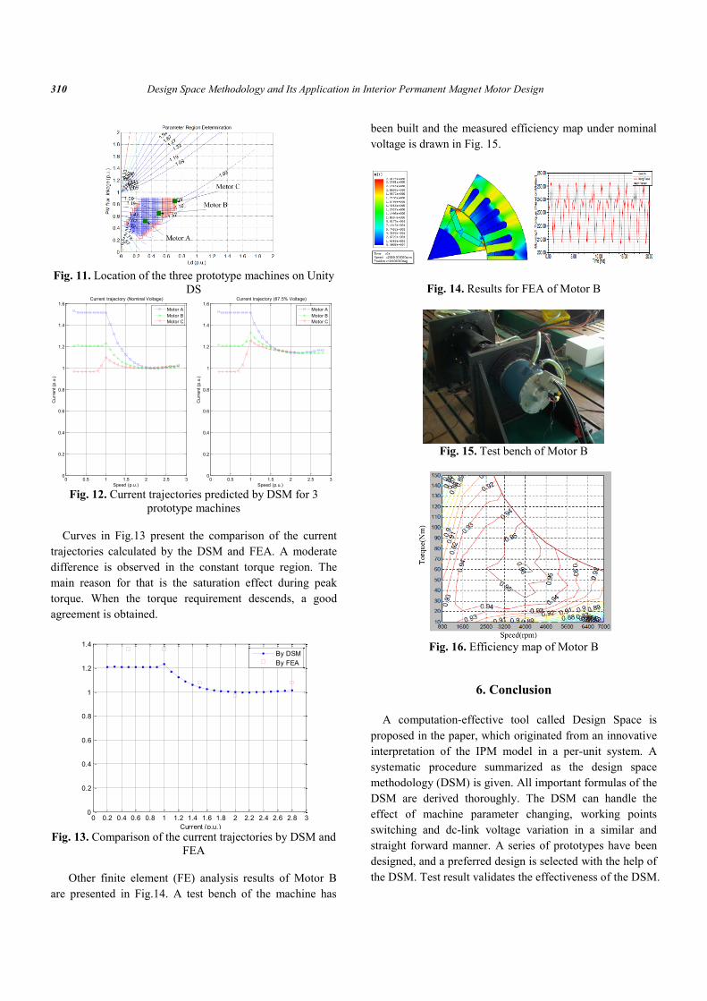
Other finite element (FE) analysis results of Motor B
are presented in Fig.14. A test bench of the machine has
been built and the measured efficiency map under nominal
voltage is drawn in Fig. 15.
Fig. 14. Results for FEA of Motor B
Fig. 15. Test bench of Motor B
Fig. 16. Efficiency map of Motor B
6. Conclusion
A computation-effective tool called Design Space is
proposed in the paper, which originated from an innovative
interpretation of the IPM model in a per-unit system. A
systematic procedure summarized as the design space
methodology (DSM) is given. All important formulas of the
DSM are derived thoroughly. The DSM can handle the
effect of machine parameter changing, working points
switching and dc-link voltage variation in a similar and
straight forward manner. A series of prototypes have been
designed, and a preferred design is selected with the help of
the DSM. Test result validates the effectiveness of the DSM.

Fan Tao, Li Qi, Wen Xuhui and Xu Longya 311
Acknowledgements
This work was supported by the Innovation Program of
Chinese Academy of Sciences (KGCX2-EW-324).
References
[1] A.M. EL-Refaie and T.M. Jahns, "Optimal flux weakening in
surface PM machines using fractional-slot concentrated
windings," IEEE Trans. on Ind. Appl., vol. 41, Issue 3, pp.
790 – 800, May/Jun. 2005.
[2] R.F. Schiferl and T.A. Lipo, "Power capability of salient pole
permanent magnet synchronous motors in variable speed
drive applications," IEEE Trans. on Ind. Appl., Vol. 26, Issue
1, pp. 115 – 123, Jan/Feb. 1990,
[3] S. Morimoto, M. Sanada and Y. Takeda, “Inverter-Driven
Synchronous Motors for Constant Power,” IEEE Industry
Applications Society Magazine, pp. 18 – 24, Nov/Dec. 1996,
[4] W.L. Soong and T.J.E. Miller, “Field-Weakening
Performance of the Five Classes of Brushless Synchronous
AC Motor Drives,” in IEE Proceedings, Electric Power
Applications, vol. 141, No. 6 Nov. 1994, pp. 331-340.
[5] Fan tao, Wen Xuhui, Meng Haiying, Longya Xu, Zhao Feng
and Liu Jun, “Development of the DMPM-based Electrical
Variable Transmission for HEV Drive,” in IEEE Proceedings
of ECCE 2009, San Jose, Sept. 2009 .
[6] Fan tao, Luo Jian, Wen Xuhui and Liao Xiaofeng. “Design
Criteria and Procedure of Interia Permanent Magnet Machine
in the Electric Vechicle Application”, in IEEE Proceedings of
ICEICE 2011,Wuhan, May 2011.
[7] Longya Xu, Fan Tao and Wen Xuhui, “Synthesis of
dimensionless indexes for IPM machine in variable speed
operations”, in IEEE Proceedings of ICEMS 2008, Wuhan,
July 2008.
[8] Soong, W.L. Reddy, P.B. El-Refaie, A.M. Jahns, T.M. and
Ertugrul, N., “Surface PM Machine Parameter Selection for
Wide Field-Weakening Applications”, in IEEE Proceedings
of IAS 2007,Sydney, July 2007.
[9] U.S. Department of Energy, "Development of Power
Electronics and Electric Motor Technology for plug-in
Hybrid Electric Vehicles, Internal Combustion Engine Hybrid
Electric Vehicles and Fuel Cell Vehicle Traction Drive
Applications", Funding Opportunity Announcement No. DE-
PS26-06NT43001-00, Sept. 22, 2006: pp. 9-10.R.
[10] A. Adnanes, R. Nilssen, and R. Rad, "Power Feed-Back
during Controller Failure in Inverter Fed Permanent Magnet
Synchronous Motor Drives with Flux Weakening", in Proc.
Of 1992 IEEE Power Elec. Spec. Conf (PESC), pp. 958-963,
1992.
Fan Tao received his B.S degree in electric
al engineering from Tsinghua University in
2004, and his M.S and PhD degrees in elect
rical engineering from the Graduate Univers
ity of the Chinese Academy of Sciences in 2
006 and 2009 respectively. His research interests are electri
c machines and drive systems of electric vehicles.
Li Qi received the B.S. degree in Electrical
engineering from HuaZhong University of
Science and Technology. Since September
2008, he has been studying in Institute of
electrical engineering of Chinese Academic
of Science. His current research interest is permanent
machine design.
Wen Xuhui received the B.S., M.S., and
Ph.D. degrees in electrical engineering from
Tsinghua University, Beijing, China, in
1984, 1987, and 1993, respectively. Since
1993, she has been with the Institute of
Electrical Engineering (IEE), Chinese Academy of Sciences
(CAS), Beijing, China, where she became an Associate
Professor in 1996 and a Professor in 1999. From 2004 to
2005, she was a Visiting Researcher with The Ohio State
University. Her research fields include power electronics,
motion control, and electric vehicle drives.
Xu Longya received the M.S. and Ph.D.
degrees in electrical engineering from the
University of Wisconsin, Madison, in 1986 and
1990, respectively. In 1990, he joined the
Department of Electrical Engineering at Ohio
State University, Columbus, where he is currently a Professor. He
has served as a consultant to many industrial companies,
including Raytheon Company, U.S. Wind Power Company,
General Motors, Ford, and Unique Mobility Inc. His research and
teaching interests include dynamic modeling and optimized
design of electrical machines and power converters for variable-
speed generating and drive systems, and application of advanced
control theory and digital signal processors in controlling motion
systems for super-high-speed operation.