Design Parameters Sessions A1.1 and A2.1

Plenary Report

C.SpieringVLVNT Workshop Amsterdam

October 2003

low bioluminescence

low bioluminescence far from big rivers

low bioluminescence far from big rivers far from inflow of other debris

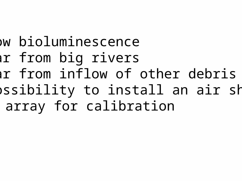
low bioluminescence far from big rivers far from inflow of other debris possibility to install an air shower array for calibration

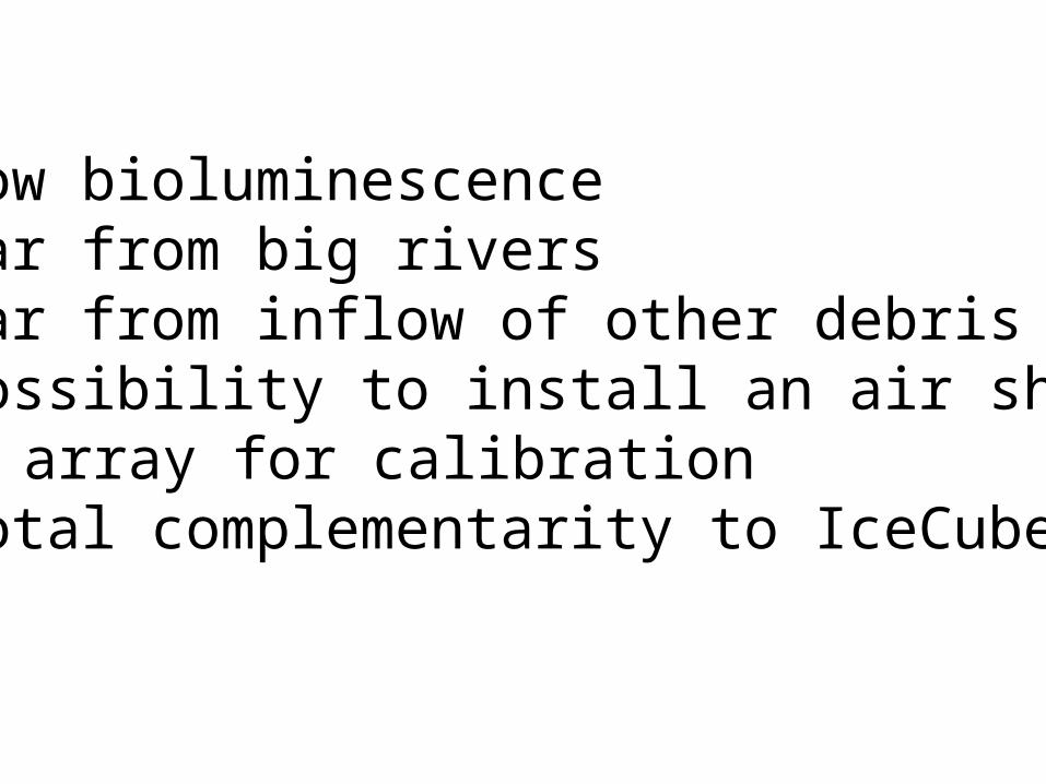
low bioluminescence far from big rivers far from inflow of other debris possibility to install an air shower array for calibration total complementarity to IceCube

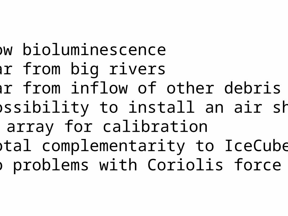
low bioluminescence far from big rivers far from inflow of other debris possibility to install an air shower array for calibration total complementarity to IceCube no problems with Coriolis force

North Pole !

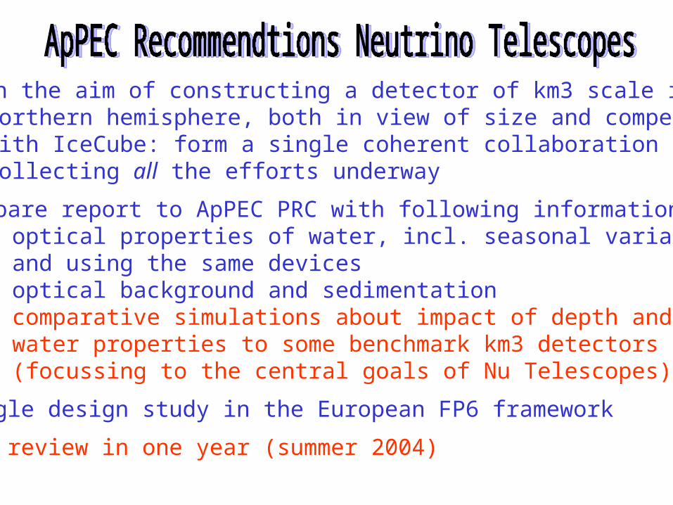
With the aim of constructing a detector of km3 scale in the Northern hemisphere, both in view of size and competition with IceCube: form a single coherent collaboration collecting all the efforts underway

Prepare report to ApPEC PRC with following informations: - optical properties of water, incl. seasonal variations and using the same devices

- optical background and sedimentation- comparative simulations about impact of depth and

water properties to some benchmark km3 detectors (focussing to the central goals of Nu Telescopes)

Single design study in the European FP6 framework

New review in one year (summer 2004)

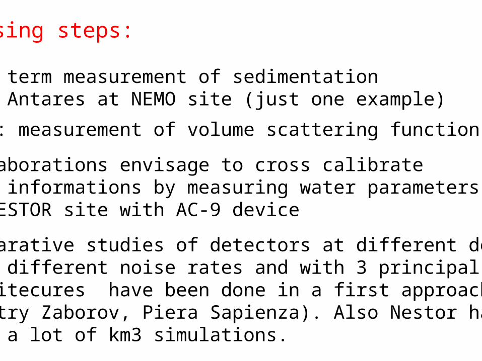
Promising steps:

- Long term measurement of sedimentation a la Antares at NEMO site (just one example)

- next: measurement of volume scattering function

- Collaborations envisage to cross calibrate site informations by measuring water parameters at NESTOR site with AC-9 device

- Comparative studies of detectors at different depths, with different noise rates and with 3 principal architecures have been done in a first approach (Dmitry Zaborov, Piera Sapienza). Also Nestor has done a lot of km3 simulations.

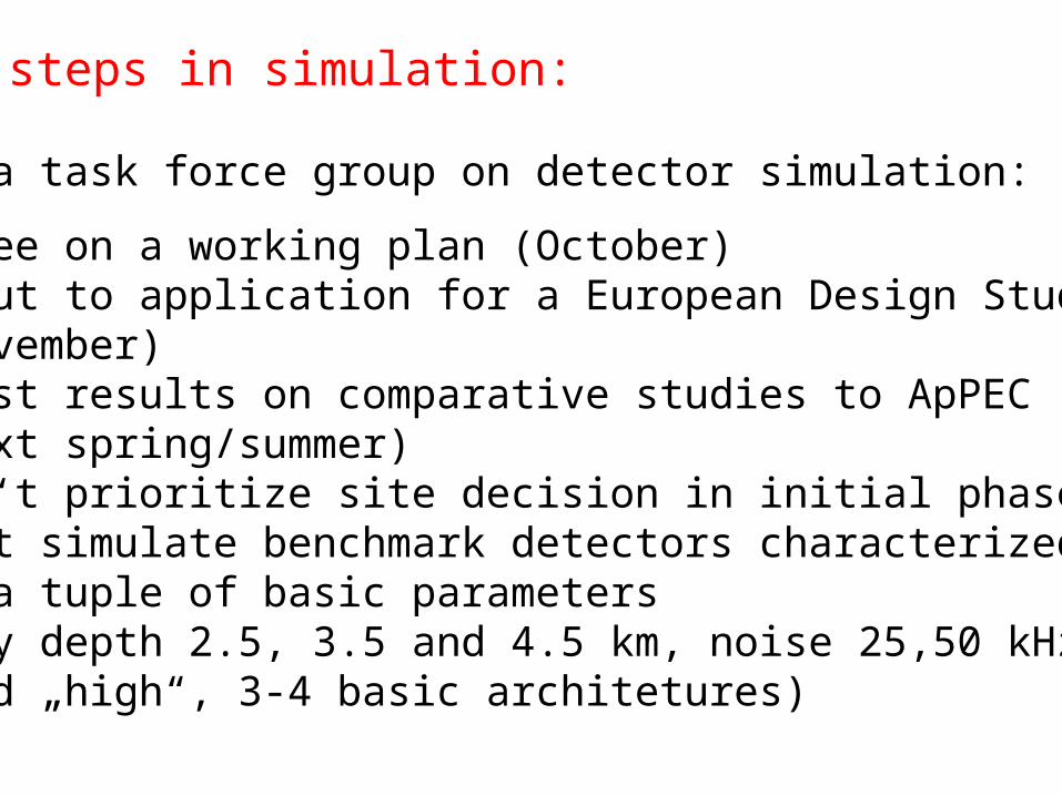
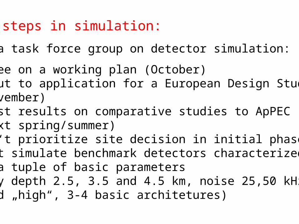
Next steps in simulation:

Form a task force group on detector simulation:

- Agree on a working plan (October)- Input to application for a European Design Study (November)- First results on comparative studies to ApPEC (Next spring/summer)- don‘t prioritize site decision in initial phase but just simulate benchmark detectors characterized by a tuple of basic parameters (say depth 2.5, 3.5 and 4.5 km, noise 25,50 kHz and „high“, 3-4 basic architetures)

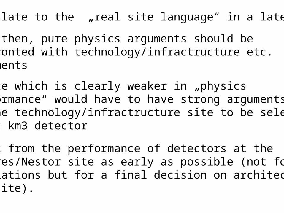
- Translate to the „real site language“ in a later step

- only then, pure physics arguments should be confronted with technology/infractructure etc. arguments

- a site which is clearly weaker in „physics performance“ would have to have strong arguments on the technology/infractructure site to be selected for a km3 detector

- Input from the performance of detectors at the Antares/Nestor site as early as possible (not for simulations but for a final decision on architectiure and site).

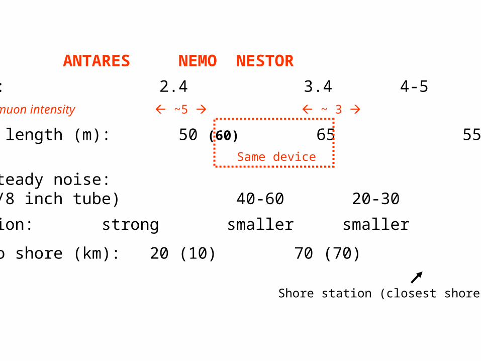
ANTARES NEMO NESTOR

Depth (km): 2.4 3.4 4-5

Factor downward muon intensity ~5 ~ 3

Absorption length (m): 50 (60) 65 55-70

External steady noise: (kHz/8 inch tube) 40-60 20-30 20-30 (10“)

Sedimentation: strong smaller smaller

Distance to shore (km): 20 (10) 70 (70) 20 (15)

Shore station (closest shore)

Same device

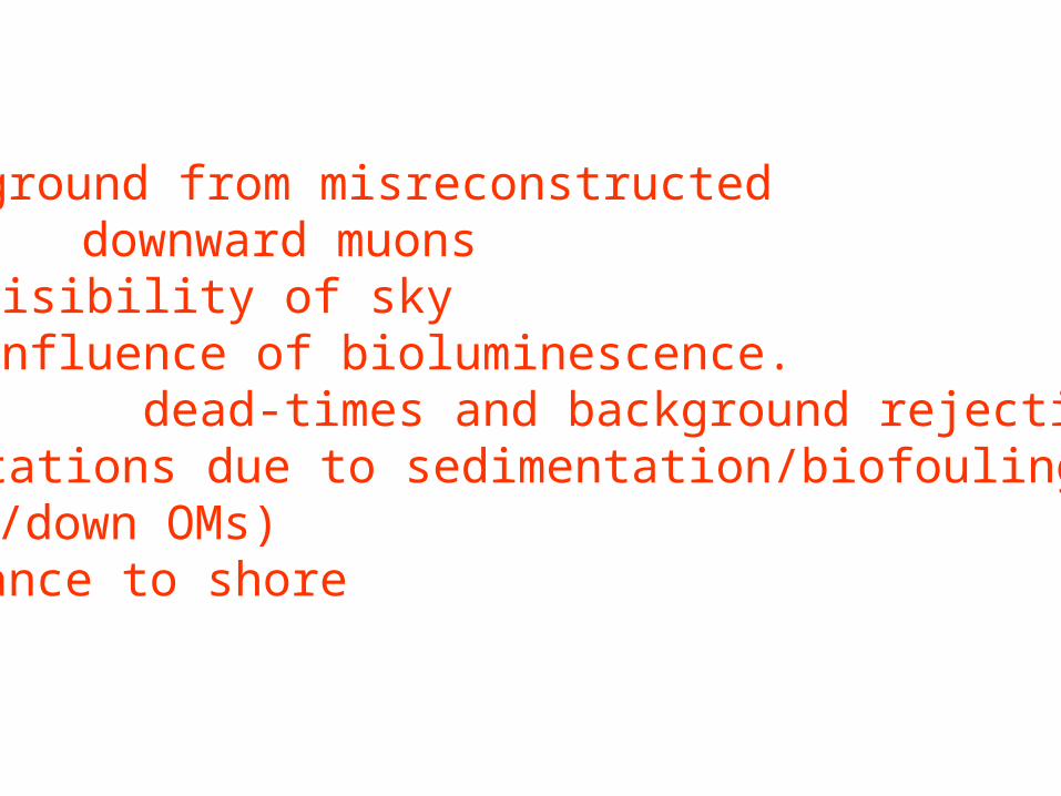
- Background from misreconstructed downward muons- Visibility of sky- Influence of bioluminescence. dead-times and background rejection- Limitations due to sedimentation/biofouling (up/down OMs)- Distance to shore

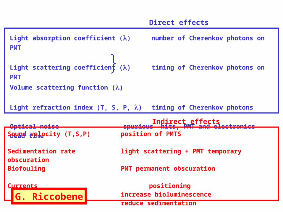
Light absorption coefficient () number of Cherenkov photons on PMT

Light scattering coefficient () timing of Cherenkov photons on PMT

Volume scattering function ()

Light refraction index (T, S, P, ) timing of Cherenkov photons

Optical noise spurious hits, PMT and electronics dead

time

Sound velocity (T,S,P) position of PMTS

Sedimentation rate light scattering + PMT temporary obscurationBiofouling PMT permanent obscuration

Currents positioningincrease bioluminescencereduce sedimentation

Indirect effects

Direct effects

G. Riccobene

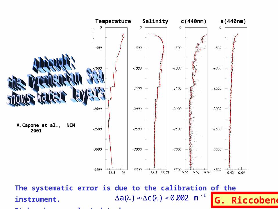
Temperature c(440nm) a(440nm)Salinity

A.Capone et al., NIM 2001

The systematic error is due to the calibration of the instrument.

It has been evaluated to be:10 002a( ) c( ) . m G. Riccobene

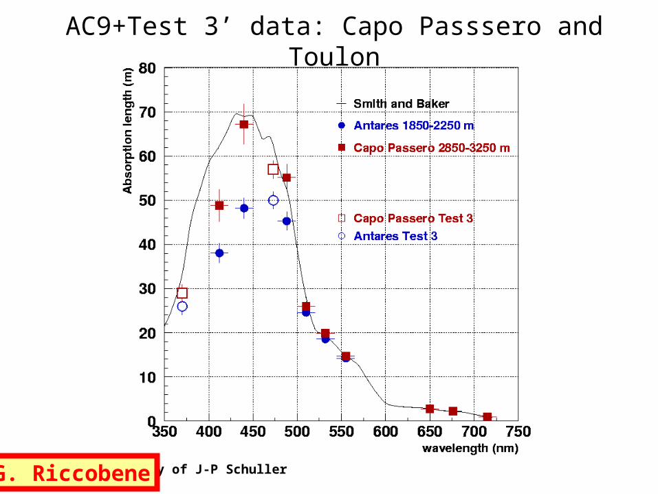
Test 3’ Data courtesy of J-P Schuller

AC9+Test 3’ data: Capo Passsero and Toulon

G. Riccobene

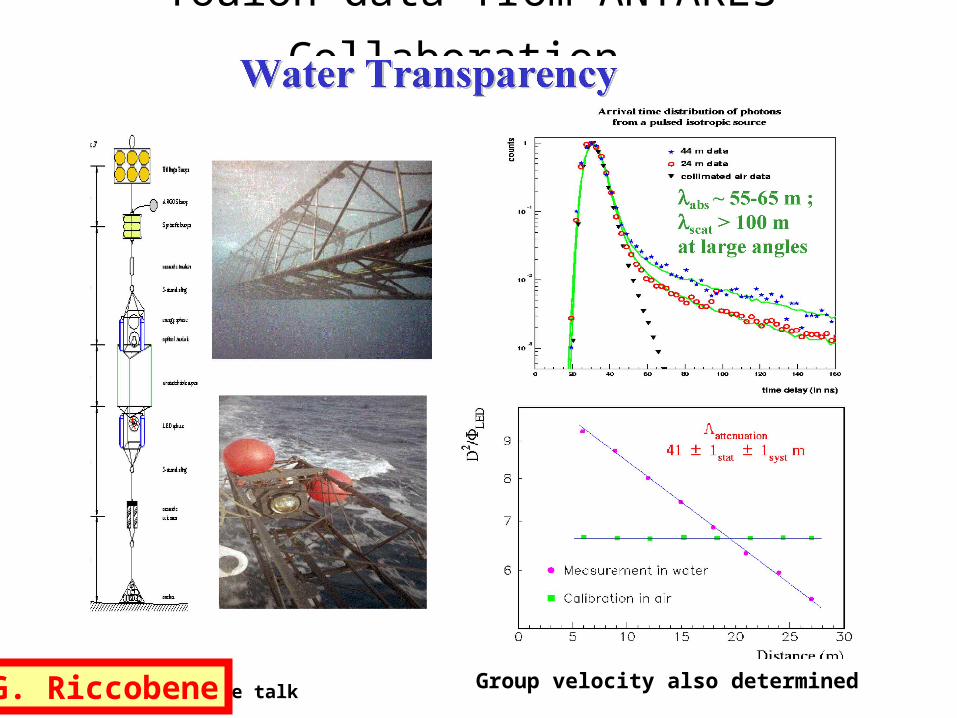
Toulon data from ANTARES Collaboration

Group velocity also determined Slide from P.Coyle talkG. Riccobene

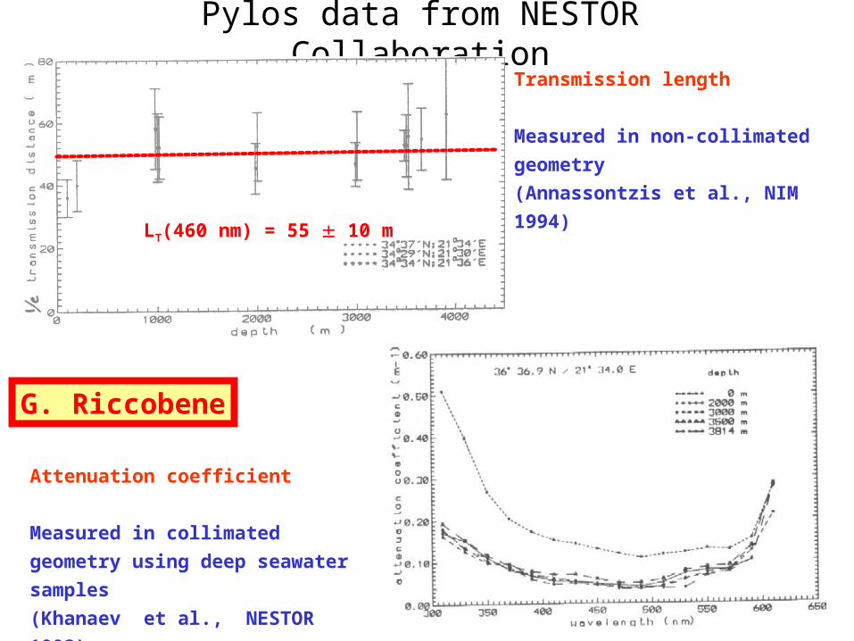
Pylos data from NESTOR CollaborationTransmission length

Measured in non-collimated

geometry

(Annassontzis et al., NIM

1994)

Attenuation coefficient

Measured in collimated

geometry using deep seawater

samples

(Khanaev et al., NESTOR 1993)

LT(460 nm) = 55 10 m

G. Riccobene

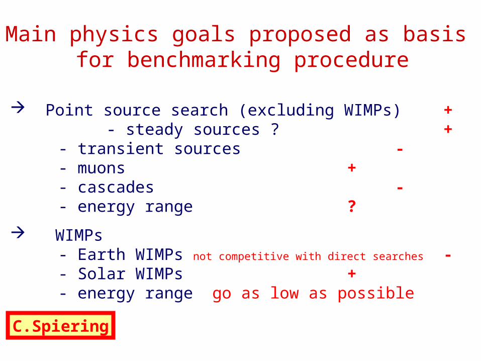
Main physics goals proposed as basis for benchmarking procedure

Point source search (excluding WIMPs) + - steady sources ? +

- transient sources -- muons +- cascades -- energy range ?

WIMPs- Earth WIMPs not competitive with direct searches -- Solar WIMPs +- energy range go as low as possible

C.Spiering

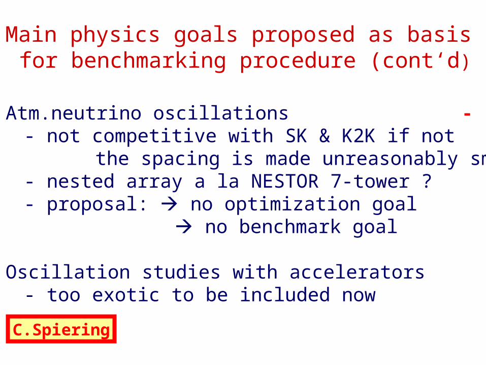
Main physics goals proposed as basis for benchmarking procedure (cont‘d)

Atm.neutrino oscillations -- not competitive with SK & K2K if not

the spacing is made unreasonably small- nested array a la NESTOR 7-tower ?- proposal: no optimization goal

no benchmark goal

Oscillation studies with accelerators -- too exotic to be included now

C.Spiering

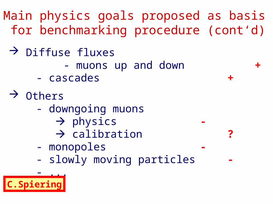
Main physics goals proposed as basis for benchmarking procedure (cont‘d)

Diffuse fluxes - muons up and down +

- cascades +

Others- downgoing muons physics - calibration ?- monopoles -- slowly moving particles -- ...

C.Spiering

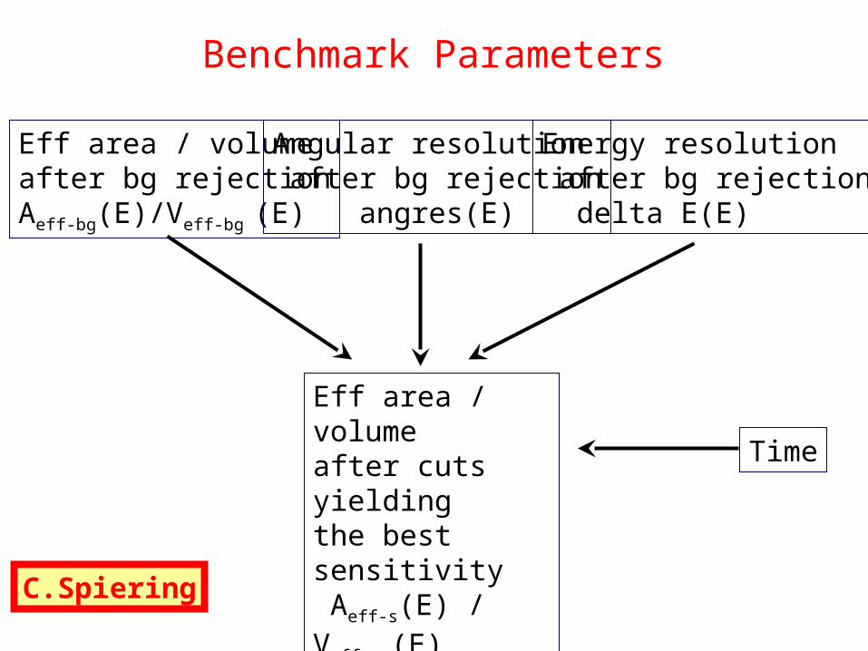
Eff area / volumeafter bg rejectionAeff-bg(E)/Veff-bg (E)

Angular resolution after bg rejection angres(E)

Energy resolution after bg rejection delta E(E)

Eff area / volumeafter cuts yielding the best sensitivity Aeff-s(E) / Veff-s (E)

Time

Benchmark Parameters

C.Spiering

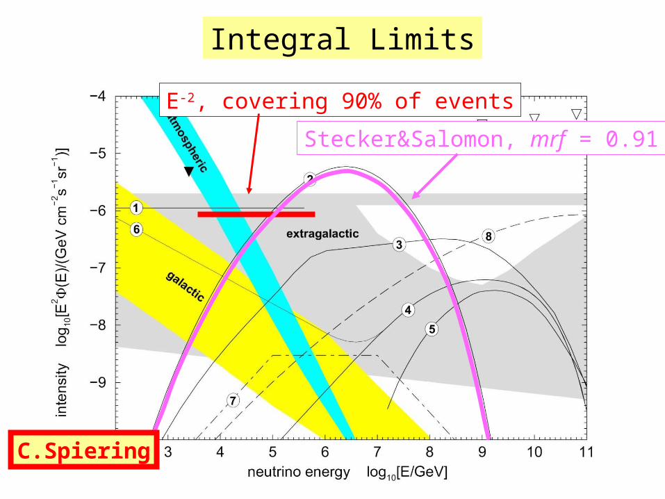
E-2, covering 90% of events

Stecker&Salomon, mrf = 0.91

Integral Limits

C.Spiering

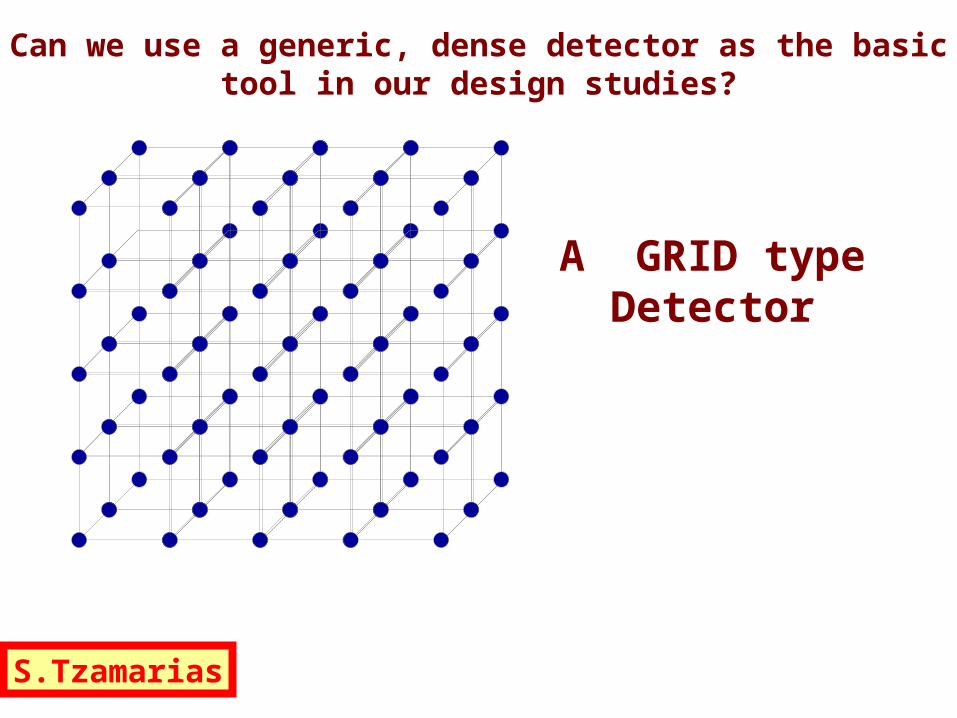
Can we use a generic, dense detector as the basic tool in our design studies?

A GRID type Detector

S.Tzamarias

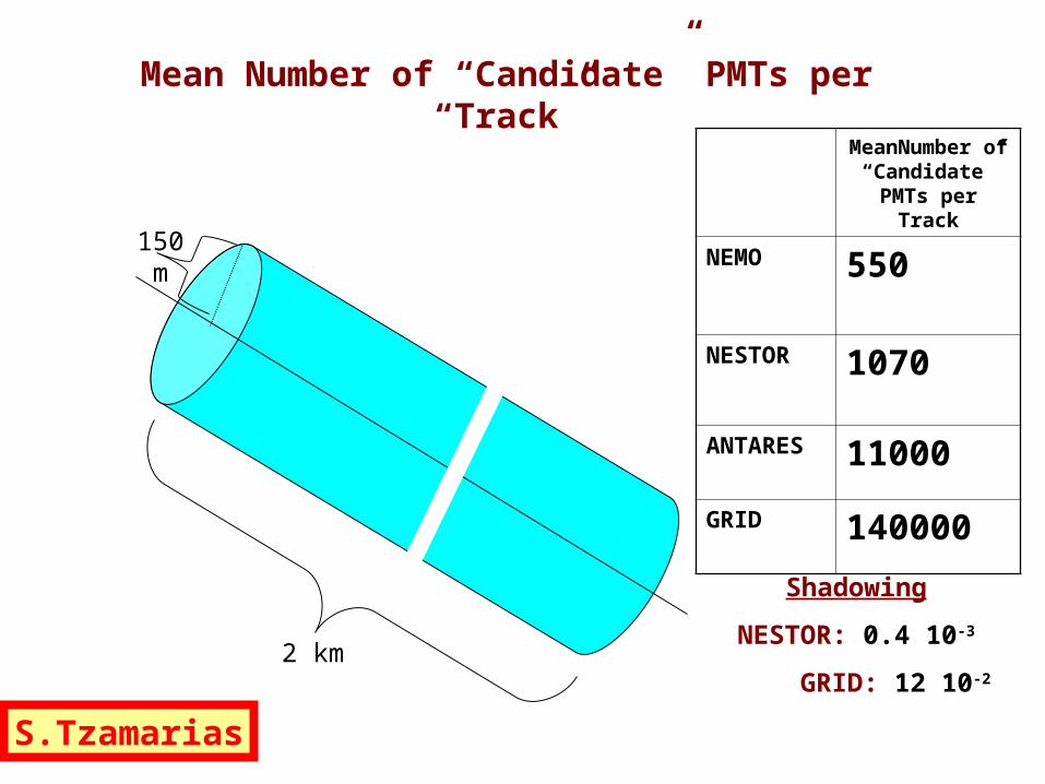
2 km

150 m

MeanNumber of

“Candidate” PMTs per

Track

NEMO 550

NESTOR 1070

ANTARES 11000

GRID 140000

Mean Number of “Candidate” PMTs per “Track”

Shadowing

NESTOR: 0.4 10-3

GRID: 12 10-2

S.Tzamarias

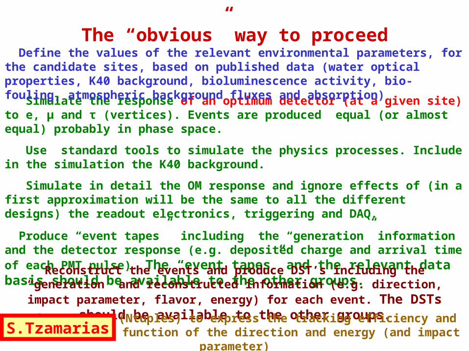
The “obvious” way to proceed

Simulate the response of an optimum detector (at a given site) to e, μ and τ (vertices). Events are produced equal (or almost equal) probably in phase space.

Use standard tools to simulate the physics processes. Include in the simulation the K40 background.

Simulate in detail the OM response and ignore effects of (in a first approximation will be the same to all the different designs) the readout electronics, triggering and DAQ.

Produce “event tapes” including the “generation” information and the detector response (e.g. deposited charge and arrival time of each PMT pulse). The “event tapes” and the relevant data basis should be available to the other groups.

Reconstruct the events and produce DST’s including the “generation” and reconstructed information (e.g. direction, impact

parameter, flavor, energy) for each event. The DSTs should be available to the other groups.Produce tables (Ntuples) to express the tracking efficiency and

resolution as a function of the direction and energy (and impact parameter)

Define the values of the relevant environmental parameters, for the candidate sites, based on published data (water optical properties, K40 background, bioluminescence activity, bio-fouling, atmospheric background fluxes and absorption)

S.Tzamarias

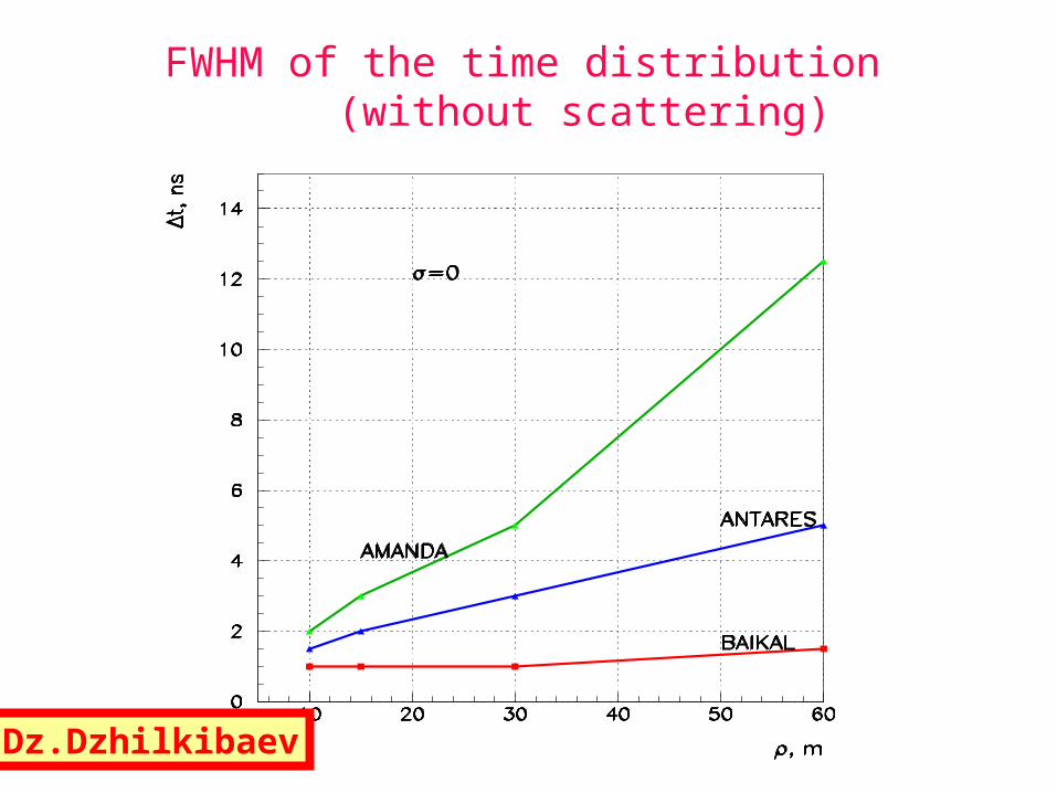
FWHM of the time distribution (without scattering)

Dz.Dzhilkibaev

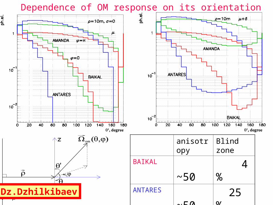
Dependence of OM response on its orientation

anisotropy Blind zone

BAIKAL ~50 4 %ANTARES ~50 25 % AMANDA ~ 4 -Dz.Dzhilkibaev

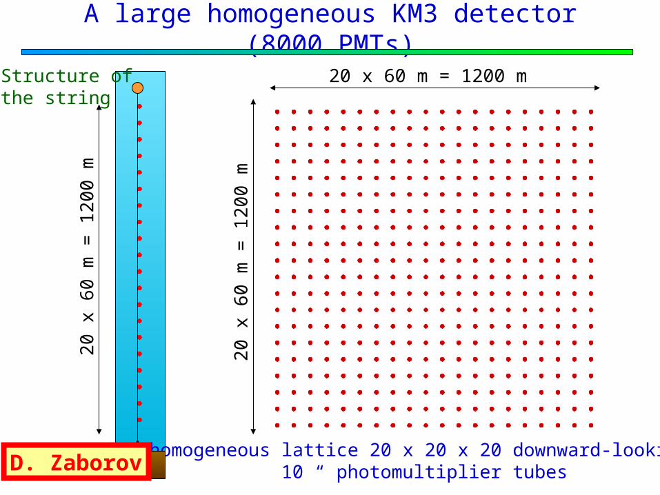
A large homogeneous KM3 detector (8000 PMTs)

homogeneous lattice 20 x 20 x 20 downward-looking 10 “ photomultiplier tubes

20 x

60

m =

120

0 m

20 x

60

m =

120

0 m

20 x 60 m = 1200 mStructure ofthe string

D. Zaborov

Top view

50 x

20

m =

100

0 m

250 m

250

m

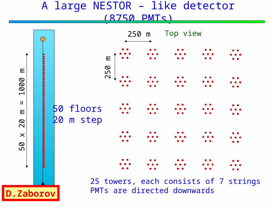
A large NESTOR – like detector (8750 PMTs)

50 floors20 m step

25 towers, each consists of 7 stringsPMTs are directed downwardsD.Zaborov

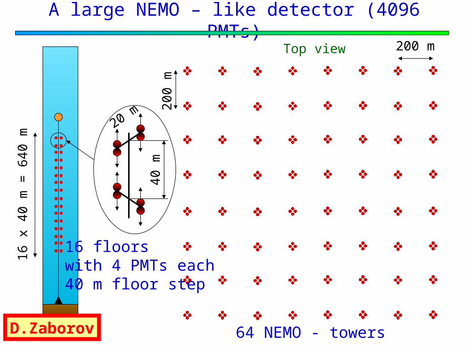
A large NEMO – like detector (4096 PMTs)200 m

200

m

16 x

40

m =

640

m

40 m

20 m

Top view

16 floorswith 4 PMTs each40 m floor step

64 NEMO - towersD.Zaborov

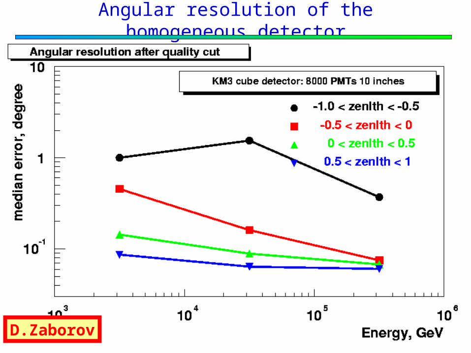
Angular resolution of the homogeneous detector

D.Zaborov

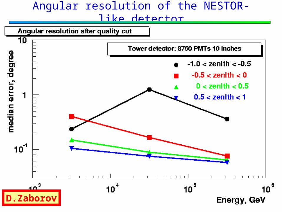
Angular resolution of the NESTOR-like detector

D.Zaborov

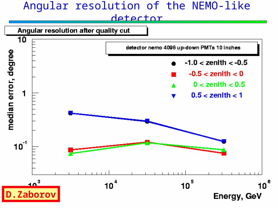
Angular resolution of the NEMO-like detector

D.Zaborov

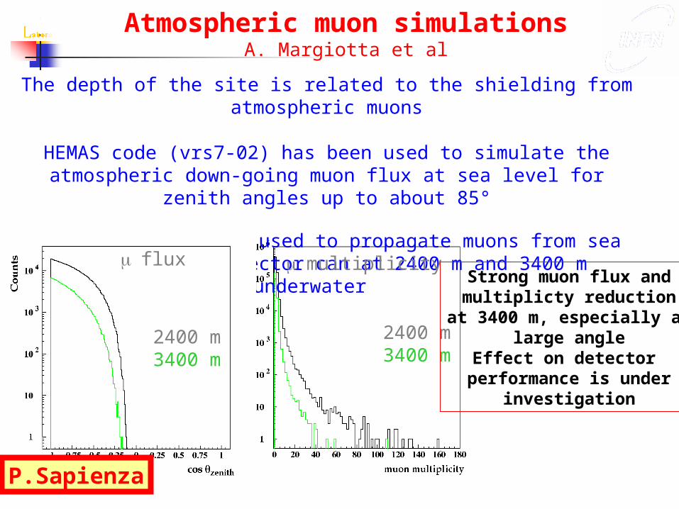
Atmospheric muon simulationsA. Margiotta et al

The depth of the site is related to the shielding from atmospheric muons

HEMAS code (vrs7-02) has been used to simulate the atmospheric down-going muon flux at sea level for zenith angles up to about 85°

MUSIC code has been used to propagate muons from sea level to the detector can at 2400 m and 3400 m underwater

2400 m3400 m

2400 m3400 m

multiplicityfluxStrong muon flux andmultiplicty reduction

at 3400 m, especially atlarge angle

Effect on detector performance is under

investigation

P.Sapienza

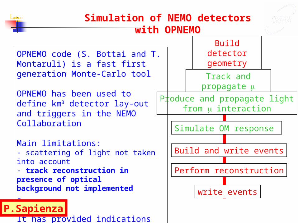
Simulation of NEMO detectors with OPNEMO

Build detector geometry

Track and propagate

Produce and propagate lightfrom interaction

Simulate OM response

Build and write events

OPNEMO code (S. Bottai and T. Montaruli) is a fast first generation Monte-Carlo tool

OPNEMO has been used to define km3 detector lay-out and triggers in the NEMO Collaboration

Main limitations:- scattering of light not taken into account- track reconstruction in presence of optical background not implemented- …

It has provided indications for the detector lay-out

Perform reconstruction

write events

P.Sapienza

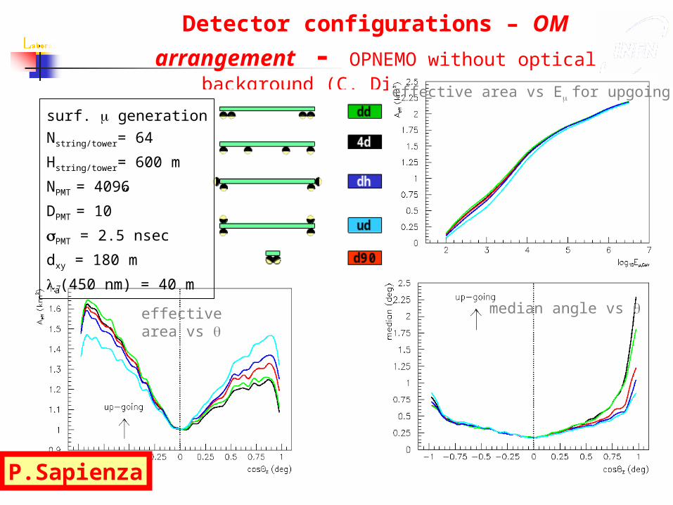
Detector configurations – OM arrangement - OPNEMO without optical background (C. Distefano et al)

effective area vs Efor upgoing

surf. generation

Nstring/tower= 64

Hstring/tower= 600 m

NPMT = 4096

DPMT = 10”

PMT = 2.5 nsec

dxy = 180 m

a(450 nm) = 40 m

effective area vs median angle vs

P.Sapienza

Simulations of NEMO detectors with the ANTARES software

package (R. Coniglione, P.S. et al)

During the ANTARES meeting held in Catania on september 2002, the ANTARES and NEMO collaboration agreed to start a stronger cooperation towards the km3.In particular, activities concerning site characterization and software were mentioned.By the end of 2002, ANTARES software was installed in Catania by D. Zaborov.

P.Sapienza

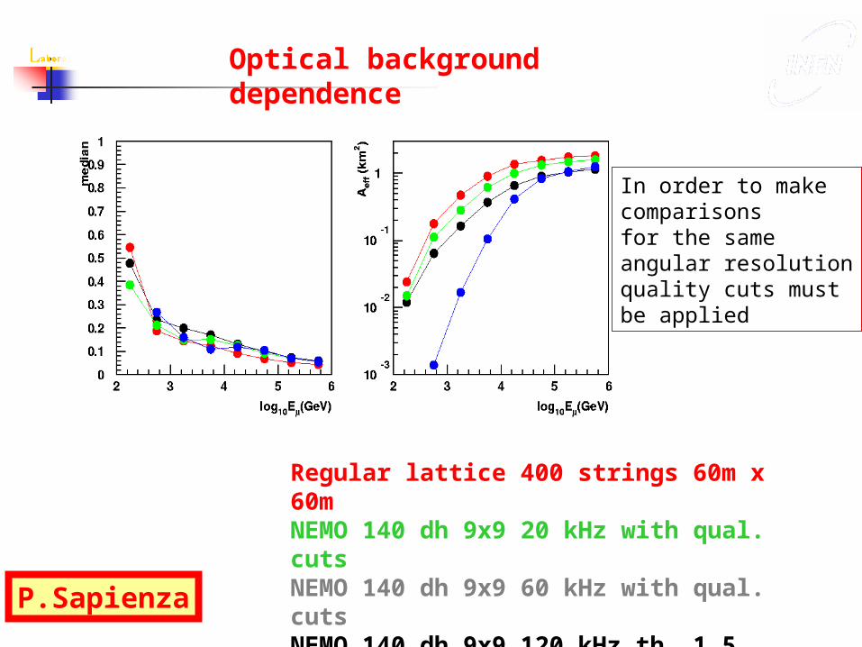
Optical background dependence

Regular lattice 400 strings 60m x 60mNEMO 140 dh 9x9 20 kHz with qual. cutsNEMO 140 dh 9x9 60 kHz with qual. cutsNEMO 140 dh 9x9 120 kHz th. 1.5 p.e. & q. c.

In order to make comparisons for the same angular resolutionquality cuts must be applied

P.Sapienza

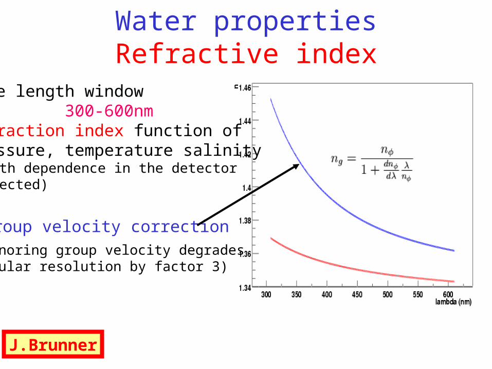
Water properties Refractive index

Wave length window 300-600nmRefraction index function of pressure, temperature salinity(depth dependence in the detectorneglected)

Group velocity correction(ignoring group velocity degradesAngular resolution by factor 3)

J.Brunner

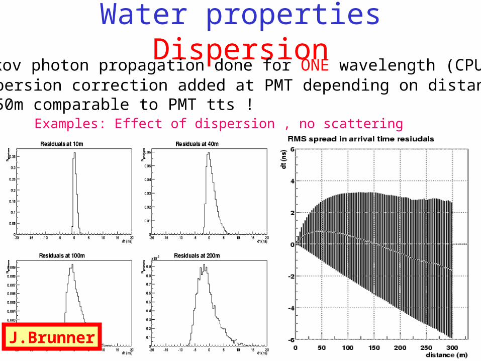
Water properties DispersionCherenkov photon propagation done for ONE wavelength (CPU time)

Dispersion correction added at PMT depending on distanceAt 50m comparable to PMT tts !

Examples: Effect of dispersion , no scattering

J.Brunner

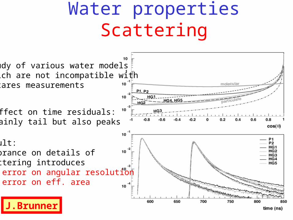
Water properties Scattering

Study of various water modelsWhich are not incompatible with Antares measurements

Effect on time residuals:Mainly tail but also peaks

Result:Ignorance on details ofScattering introduces30% error on angular resolution 10% error on eff. area

J.Brunner

• Full simulation chain operational in Antares

• External input easily modifiable

• Scalable to km3 detectors, different sites

• Could be used as basis for a km3 software tool box

J.Brunner

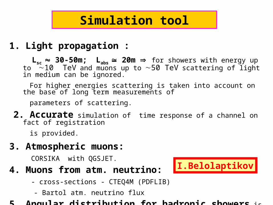
1. Light propagation :

Lsc 30-50m; Labs 20m for showers with energy up to 10 TeV and muons up to 50 TeV scattering of light in medium can be ignored.

For higher energies scattering is taken into account on the base of long term measurements of

parameters of scattering.

2. Accurate simulation of time response of a channel on fact of registration

is provided.

3. Atmospheric muons: CORSIKA with QGSJET.

4. Muons from atm. neutrino:

- cross-sections - CTEQ4M (PDFLIB)

- Bartol atm. neutrino flux

5. Angular distribution for hadronic showers is the same as for el.-m. showers.

Simulation tool

I.Belolaptikov

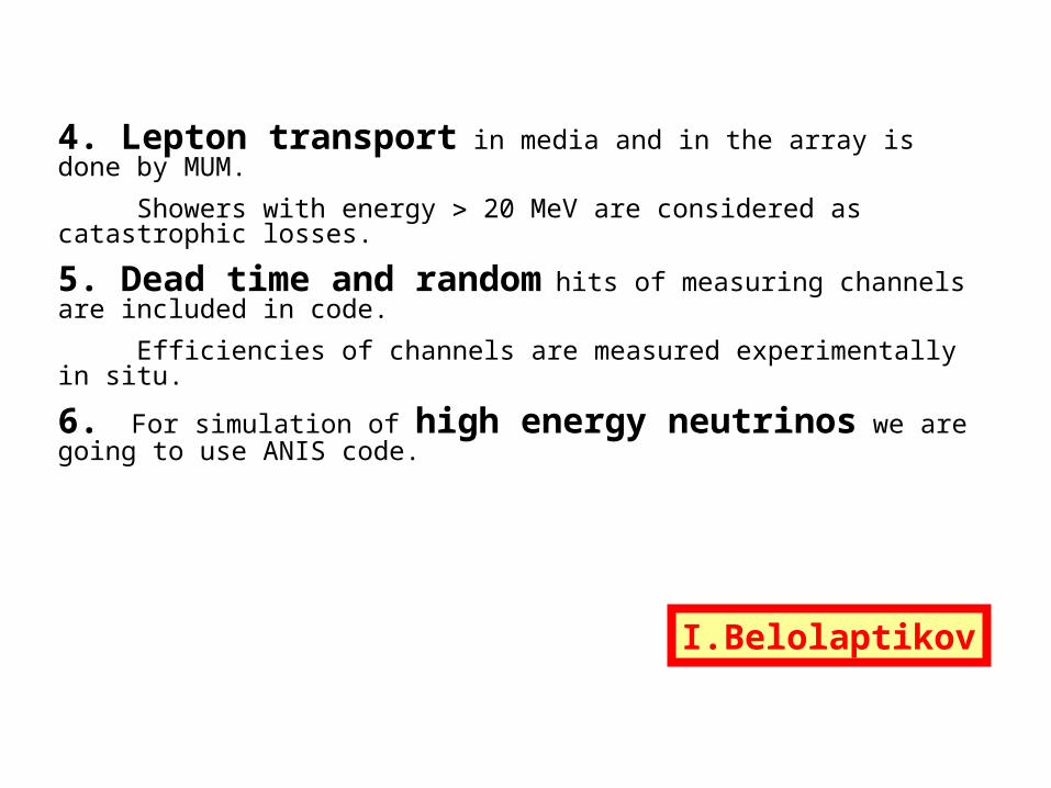
4. Lepton transport in media and in the array is done by MUM.

Showers with energy 20 MeV are considered as catastrophic losses.

5. Dead time and random hits of measuring channels are included in code.

Efficiencies of channels are measured experimentally in situ.

6. For simulation of high energy neutrinos we are going to use ANIS code.

I.Belolaptikov

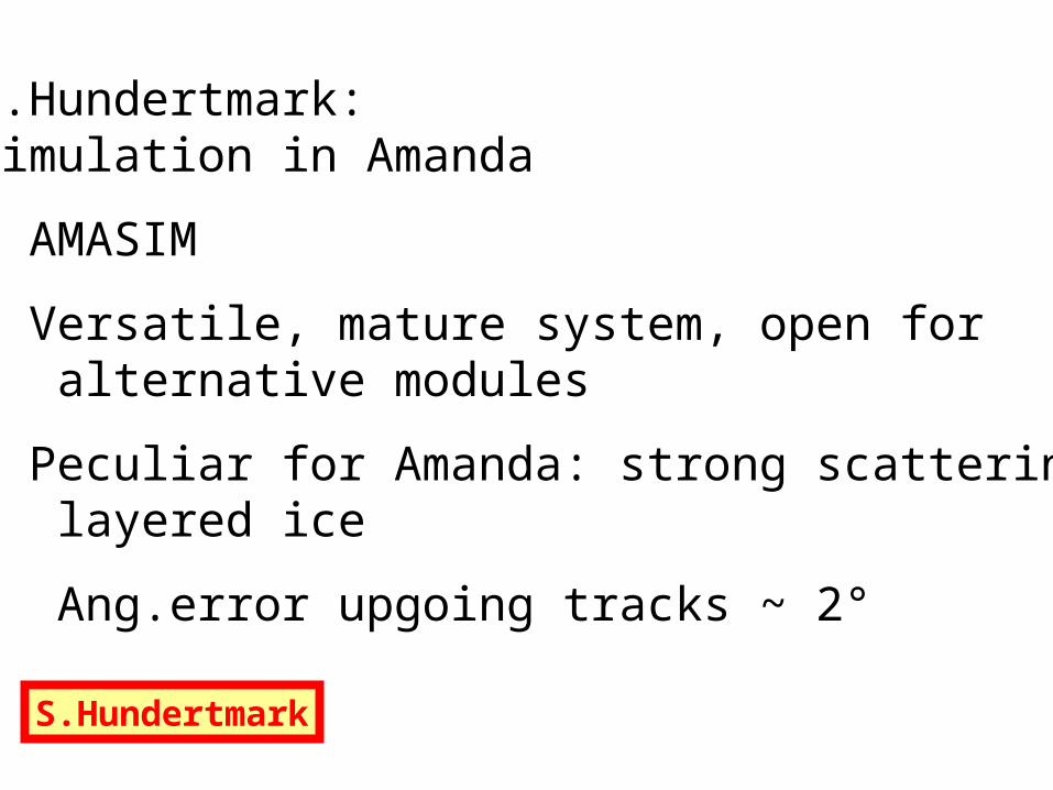
S.Hundertmark: Simulation in Amanda

- AMASIM

- Versatile, mature system, open for alternative modules

- Peculiar for Amanda: strong scattering layered ice

- Ang.error upgoing tracks ~ 2°

S.Hundertmark

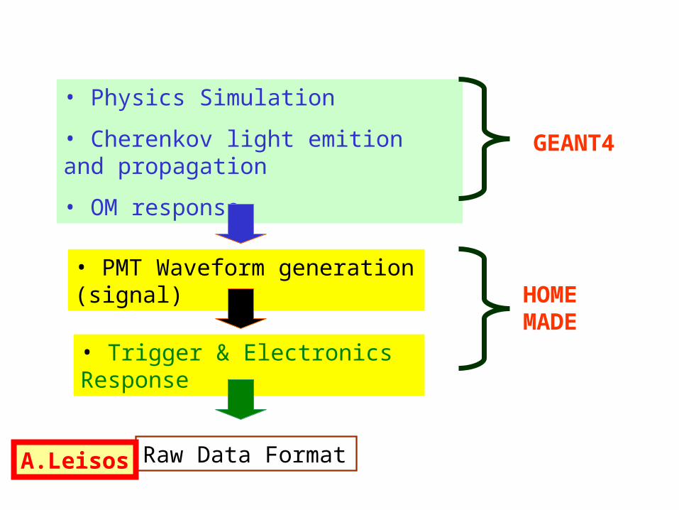
• Physics Simulation

• Cherenkov light emition and propagation

• OM response

• PMT Waveform generation (signal)

• Trigger & Electronics Response

Raw Data Format

GEANT4

HOME MADE

A.Leisos

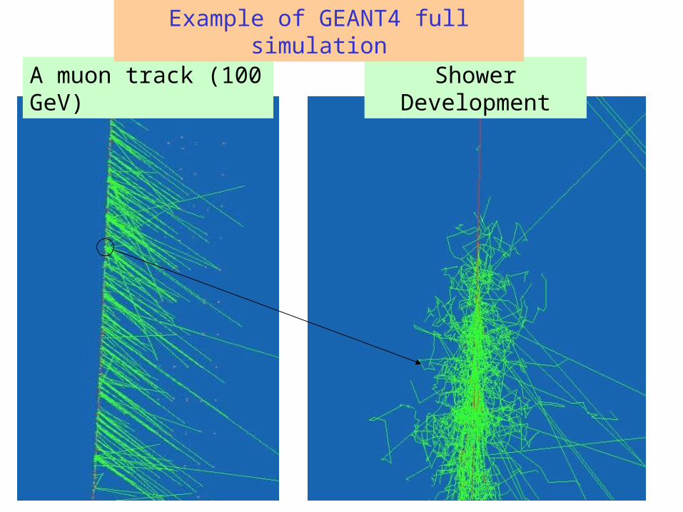
A muon track (100 GeV) Shower Development

Example of GEANT4 full simulation

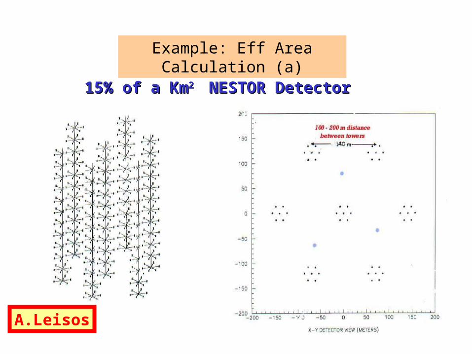
Example: Eff Area Calculation (a)

15% of a Km15% of a Km2 2 NESTOR Detector NESTOR Detector

A.Leisos

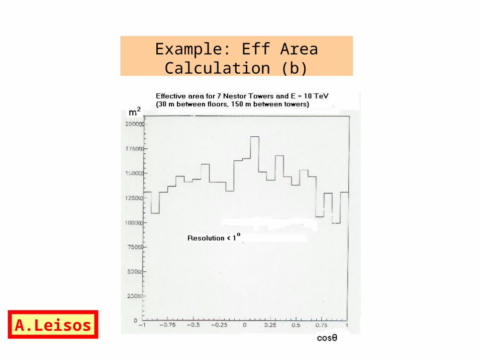
Example: Eff Area Calculation (b)

A.Leisos

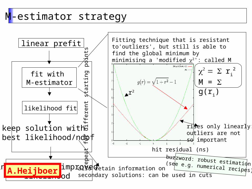
M-estimator strategy

linear prefit

likelihood fit

repe

at f

or d

iffe

rent

sta

rtin

g po

intsfit with

M-estimator

final fit with improved likelihood

keep solution withbest likelihood/ndof

Fitting technique that is resistant to'outliers', but still is able to find the global minimum byminimising a 'modified 2': called M

hit residual (ns)

rises only linearly:outliers are notso important

r2

ri2

M = g(ri)

buzzword: robust estimation(see e.g. numerical recipes)also retain information onsecondary solutions: can be used in cuts

A.Heijboer

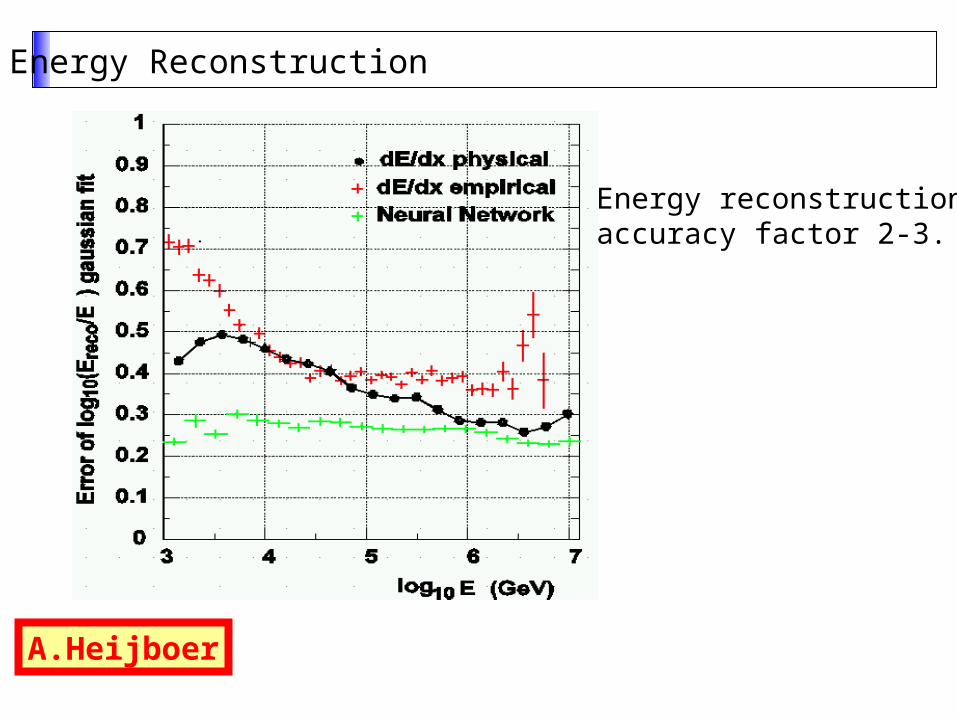
Energy Reconstruction

Energy reconstructionaccuracy factor 2-3.

A.Heijboer

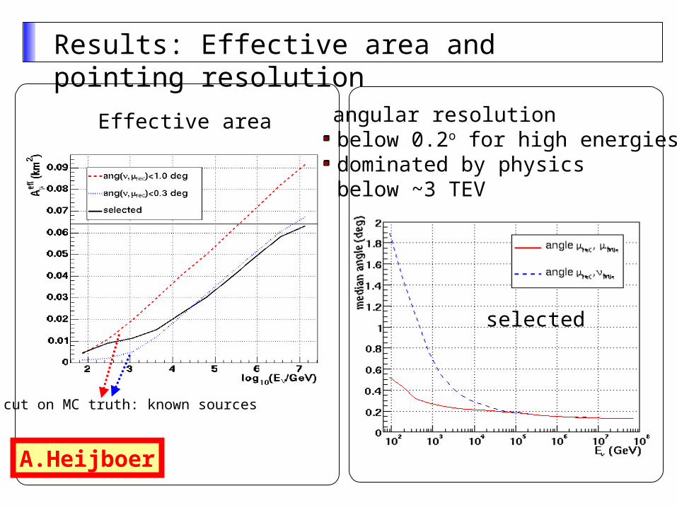
angular resolutionbelow 0.2o for high energiesdominated by physics below ~3 TEV

Results: Effective area and pointing resolution

Effective area

cut on MC truth: known sources

selected

A.Heijboer

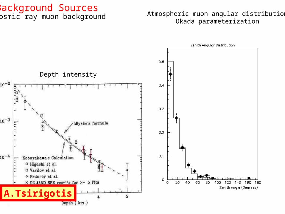
Depth intensity curve

Background SourcesCosmic ray muon background Atmospheric muon angular distribution

Okada parameterization

A.Tsirigotis

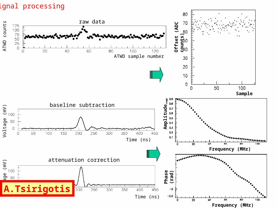
Signal processing

Frequency (MHz)

Frequency (MHz)

Ph

ase

(rad

)A

mp

litu

de

raw data

baseline subtraction

attenuation correction

Off

s et

(AD

C c

oun

ts)

Sample

AT

WD

co

un

ts

ATWD sample number

Vo

ltag

e (

mV

)

Time (ns)

Vo

ltag

e (

mV

)

Time (ns)A.Tsirigotis

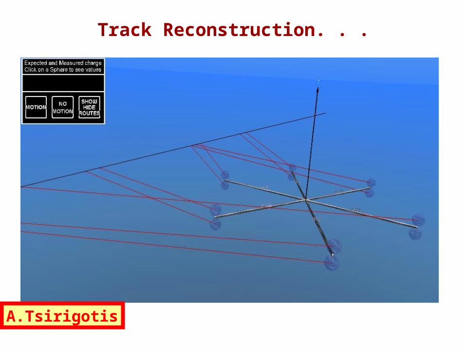
Track Reconstruction. . .

A.Tsirigotis

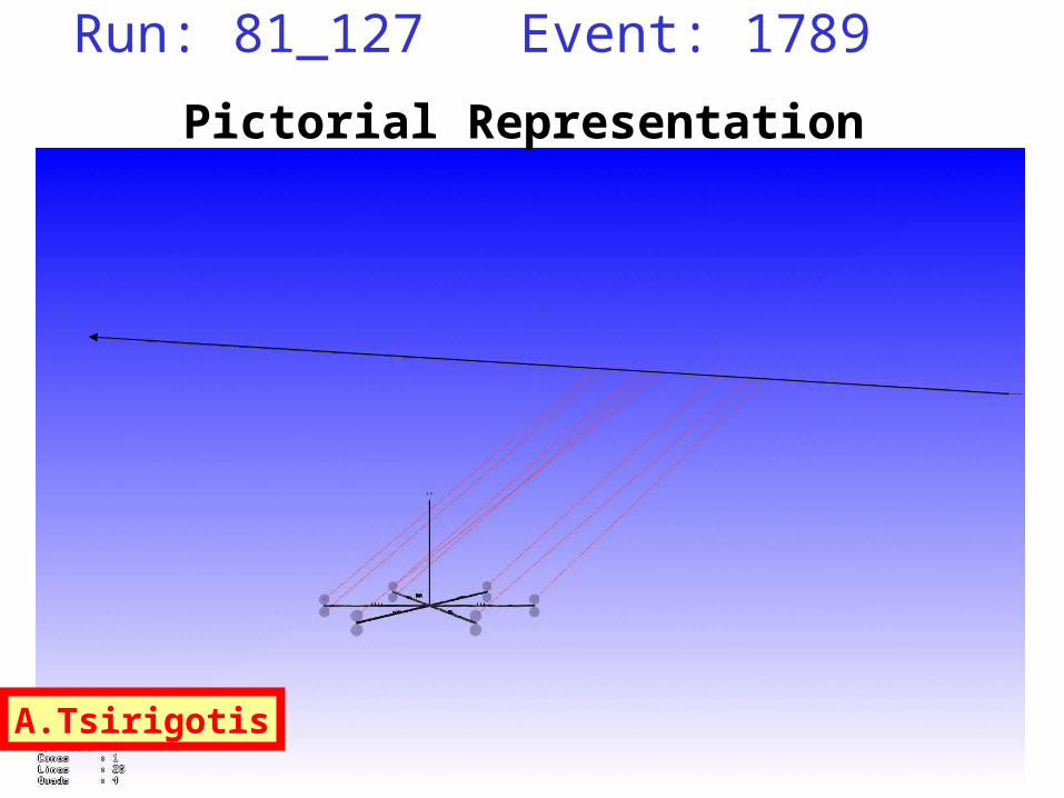
Run: 81_127 Event: 1789

Pictorial Representation

A.Tsirigotis

I.Belolaptikov: Reconstruction in Baikal

- Ang.error upgoing tracks ~ 3°

- „Allowed region“ allowed theta, phi regions from time differences between pairs of OMs (no fit)

I.Belolaptikov

C.Wiebusch: Reconstruction in Amanda

- Critical due to light scattering- appropriate likelihood („Pandel“) + clever cuts effective bg reduction, ang. error for upgoing tracks ~ 2°- Improvements: likelihood parametrization, layered ice, include waveform

C.Wiebusch

Summary

Much known about water properties – presumablyenough for detector optimization and site comparison

Cross calibration measurements done/underwayfor Antares/Nemo sites, planned to include Nestor site.

Lot of comparative simulations done in all three collaborations.

Wide spectrum of tools for simulation and reconstruction.Many standard programs common to two or even all threecollaborations (Corsika/Hemas, MUM/Music, Geant 3/4, ....)

May also use tools of Amanda/Baikal

Seems to be not too difficult to converge to tocommon simulation framework for optimization

Next steps in simulation:

Form a task force group on detector simulation:

- Agree on a working plan (October)- Input to application for a European Design Study (November)- First results on comparative studies to ApPEC (Next spring/summer)- don‘t prioritize site decision in initial phase but just simulate benchmark detectors characterized by a tuple of basic parameters (say depth 2.5, 3.5 and 4.5 km, noise 25,50 kHz and „high“, 3-4 basic architetures)