Embed Size (px)
Citation preview

Design of wind farm layout with non-uniform turbines using fitnessdifference based BBO
Jagdish Chand Bansal
South Asian University, New Delhi, India
Pushpa Farswan
South Asian University, New Delhi, India
Atulya K. Nagar
Liverpool Hope University. UK.
Abstract
Biogeography-based optimization (BBO) is an emerging meta-heuristic algorithm. BBO is inspired
from the migration of species from one island to another. This study presents the solution of the
wind farm layout optimization problem with wind turbines having non-uniform hub heights and rotor
radii using BBO and an improved version of BBO. This study proposes an improved version of BBO,
Fitness Difference Based BBO (FD-BBO). FD-BBO is obtained by incorporating the concept of fitness
differences in original BBO. First, in order to justify the superiority of FD-BBO over BBO, it is tested
over 15 standard test problems of optimization. The numerical results of FD-BBO are compared with
the original version of BBO and an advanced version of BBO, Blended BBO (BBBO). Through graphical
and statistical analyses, FD-BBO is established to be an efficient and accurate algorithm. The BBO,
BBBO and FD-BBO are than applied to solve the wind farm layout optimization problem. In the
considered problem, not only the location of the wind turbines but hub heights and rotor radii are also
taken as decision variables. Two cases of the problems are dealt: 26 turbines in the farm size of 2000m
× 2000m and 30 turbines in the farm size of 2000m × 2000m. Numerical results are compared with
earlier published results and that of original BBO and Blended BBO. It is found that FD-BBO is the
better approach to solving the problem under consideration.
Keywords: Wind farm layout, Wind turbine, Hub height, Rotor radius, Biogeography-based
optimization, Fitness difference
1. Introduction
Now a days energy is very important part of our necessity. Energy is becoming our inevitability in
daily routine. Availability of energy is a very critical issue for future needs. Technologies are promot-
ing renewable energy. Wind energy has been the fastest growing source of renewable energy from the
Email addresses: [email protected] (Jagdish Chand Bansal), [email protected] (Pushpa Farswan),[email protected] (Atulya K. Nagar)
Preprint submitted to Elsevier May 24, 2018

twentieth century. Maximization of wind energy is the most promising area of research in the field of
renewable energy. In this study, we have considered wind energy system for maximization of energy
production with the help of non-conventional optimization techniques. The power output of wind farm
depends on the locations, hub heights and rotor radii of wind turbines. There are lots of studies done
in these directions. The power output of wind farm is sensitive to other parameters also. But in this
study, we have considered only three parameters of wind turbines such as wind turbine location, hub
height and rotor radius which affects the energy production significantly. The main concern of the study
is to increase the power output of wind farm. In this regard, we are maximizing the energy output
with three parameters of wind turbines. Many non-conventional approaches have been applied to the
problems related to wind energy systems.
Mosetti et al. [1] used a non-conventional optimization algorithm (genetic algorithms) to extract max-
imum energy output corresponding to the minimum installation cost. They used 100 square cells as
possible locations for the wind turbines. Grady et al. [2] also used a genetic algorithms to find the
optimal position of wind turbines as well as the limit of the maximum number of turbines for the con-
sidered wind farm of size (2km × 2km). Marmidis et al. [3] introduce Monte Carlo simulation in wind
park optimization system to produce maximum energy with minimum installation cost. They compared
their findings with earlier studies [1, 2]. Acero et al. [4] maximize the energy production by optimizing
the placement of wind turbines on a straight line. They considered Jensen’s wake model [5] and two
optimization techniques (simulated annealing and genetic algorithms) used in their study. Mittal [6]
developed a code for wind farm layout optimization using the genetic algorithm (WFLOG) to finding
optimal position of wind turbines in the given wind farm, so that cost per power minimizes. In that
study, considered cell size was 1m×1m rather than 200m×200m used in [1, 2]. Gonzalez et al. [7] used
a more realistic integral wind farm cost model that is based on a real life cycle cost approach. They
introduced evolution approach to optimize the wind farm layout. Chowdhury et al. [8] proposed a new
methodology the unrestricted wind farm layout optimization (UWFLO), to find optimal layout of the
wind farm along with the selection of wind turbines corresponding to several rotor diameters. They
used particle swarm optimization technique in their proposed study. Chen et al. [9] applied genetic
algorithms to find the optimal layout of the wind farm corresponding to two possible hub heights (50m
and 78m) of wind turbines. Park et al. [10] incorporated sequential convex programming for maximiz-
ing power production of the wind farm. Chen et al. [11] introduced wind turbine layout optimization
corresponding to multiple hub heights of the wind turbines using the greedy algorithm. Bansal et al.
[12] proposed optimal wind farm layout using BBO algorithm. They also recommended the maximum
number of wind turbines which can be accommodated in a wind farm of given size. Recently S. Rehman
et al. proposed a variant of cuckoo search algorithm [13] by incorporating a heuristic-based seed solution
for better wind farm layout design [14]. In [15], Vasel et al. explored hub height optimization in their
study and recommended multiple hub height turbines to maximize energy annually.
In this study, we apply a modified BBO algorithm to find wind farm layout with non-uniform hub
2

heights and rotor radii. Biogeography-based optimization (BBO) is a nature inspired meta-heuristic
algorithm based on the migration of species among islands. BBO is recently introduced by Dan Simon
in 2008 [16]. BBO is popular among researchers due to few control parameter and its efficiency. This
motivated the researchers to develop BBO algorithm to solve complex real-world optimization prob-
lems. There have been significant development in BBO algorithm by improving and introducing new
operators. Some improved migration [17, 18, 19, 20, 21, 22, 23], mutation [24, 25] and new operators
[26, 27] are developed earlier. Ma et al. [17] proposed Blended BBO (BBBO) to handle constrained
optimization problems. In BBBO, information is blended, i.e. immigrating island accepts the informa-
tion (feature) from itself and emigrating island. Feng et al. [18] proposed an improved BBO (IBBO)
by improving migration operator. Xiong et al. [19] proposed polyphyletic BBO (POLBBO) by intro-
ducing polyphyletic migration operator. Wang et al. [20] introduced the krill herd algorithm with new
migration operator in BBO. Lohakare et al. [24] proposed a memetic algorithm named as aBBOmDE.
In aBBOmDE, the convergence speed of BBO is accelerated by incorporating the mutation operator of
DE. Simon et al. [26] proposed Linearized BBO (LBBO) to solving non-separable problems. In LBBO,
a local search operator is introduced with periodic re-initialization to make the algorithm appropriate
for global optimization in a continuous search space. Bansal et al. [27] proposed DisruptBBO (DBBO)
by introducing new operator in BBO algorithm to improve its exploration and exploitation capability.
Although, various variants of BBO have developed and most of the developments are related to the
tuning of migration and mutation operators of BBO algorithm. However, this study gives new insights
into developing the performance of BBO algorithm. In this study, we introduce the fitness difference
strategy in BBO algorithm (given in section 3). The so developed Fitness Difference based BBO (FD-
BBO) algorithm and proposed approach is then applied to solve wind energy optimization problem with
non uniform wind turbines. As a future study, different nature inspired algorithm such as artificial bee
colony [28], spider monkey optimization [29], water Cycle Algorithm [30] and particle swarm optimiza-
tion [31] etc. can also be applied to solve wind farm layout optimization problem with non uniform
turbines.
Rest of the paper is organized as follows: Section 2 describes the basic BBO algorithm. The discussion
of proposed Fitness Difference based BBO (FD-BBO) approach and the numerical experiments are
given in section 3. In section 4, the description of wind farm layout optimization problem is given and
this section also discusses the various results of wind farm layout solved using proposed BBO, basic
BBO and BBBO. The paper is concluded in section 5.
2. Biogeography-Based Optimization
Biogeography is the study of geographical distribution of biological organism in geographic space.
The mathematical model of biogeography is modeled by Robert Mac Arther and Edward Wilson. The
model describes the migration of species from one island to another island, the extinction of existing
species from the island and the arrival of new species in the island [32]. However, very recently a
3

new population-based evolutionary technique has been proposed based on biogeography theory and it
has been named as the Biogeography-based optimization (BBO) [16]. BBO is a technique inspired by
migration of species within islands [32]. BBO procedure is the design of population-based optimization
procedure that can be potentially applied to optimize many engineering optimization problems. In
biogeography model, the fitness of a geographical area (or island, or habitat) is evaluated by habitat
suitability index (called HSI). Higher or lower HSI habitats correspond to higher or lower suitability of
species to survive in the islands. Therefore, high HSI and low HSI corresponds to the large and small
number of species, respectively. The variables that characterize the habitability are called suitability
index variables (SIV s) e.g. rainfall, temperature, vegetation etc. The migration of species from one
habitat to another habitat is mainly governed by two parameters, immigration rate (λ) and emigration
rate (µ). Where λ and µ are the functions of the number of species in a habitat. Fig. 1 shows the
relation between the number of species and migration rates (λ and µ) [32, 16]. In model given in
Fig. 1 shows a special case i.e. maximum immigration rate (I) and maximum emigration rate (E) are
equal. From the model given in Fig. 1, it is clear that if there are zero species on the habitat, then
maximum immigration to habitat will occur and if there are the maximum number of species (Smax)
on the habitat, then maximum emigration from habitat will happen. Therefore, for the small number
of species, there is more possibility of immigration of species from another habitat and less possibility
of emigration of species from this habitat to another habitat. In the equilibrium state, immigration and
emigration of species are same and in this state, the number of species is denoted by S0.
Figure 1: Relation between number of species and migration rate [16]
4

Let us assume that Ps(t) is the probability given for s species in the habitat at any time t.
Ps(t+ ∆t) = Ps(t)(1− λs∆t− µs∆t) + Ps−1λs−1∆t+ Ps+1µs+1∆t (1)
Where λs and µs stand for immigration and emigration rate, respectively when there are s species in
the habitat.
From the Eq. 1, one of the following conditions must hold for s species in the habitat at time t+∆ t.
1. If there were s species in the habitat at time t, then there is no immigration and emigration
occurred between time t and t+∆t.
2. If there were (s − 1) species in the habitat at time t, then only one species immigrated between
time t and t+∆t.
3. If there were (s + 1) species in the habitat at time t, then only one species emigrated between
time t and t+∆ t.
For ignoring the probability of more than one immigration or emigration, ∆t is considered very small.
Letting ∆t −→ 0
Ps =
−(λs + µs)Ps + µs+1Ps+1, s = 0
−(λs + µs)Ps + λs−1Ps−1 + µs+1Ps+1, 1 ≤ s ≤ smax − 1
−(λs + µs)Ps + λs−1Ps−1, s = smax
(2)
Let us define λn and µn are maximum immigration and emigration rate. Smax is the maximum possible
number of species in the habitat. Therefore, we can obtain a matrix relation executing the dynamic
equations of the probabilities of the number of species in the habitat.
P0
P1
.
.
.
.
.
.
PSmax
=
−(λ0 + µ0) µ1 0 · · · 0
λ0 −(λ1 + µ1) µ2 · · ·...
.
.
.. . .
. . .. . .
.
.
.
.
.
.. . . λn−2 −(λn−1 + µn−1) µn
0 · · · 0 λn−1 −(λn + µn)
P0
P1
.
.
.
.
.
.
PSmax
(3)
BBO procedure is based on two simple biogeography concepts migration and mutation. BBO algorithm
is designed as each habitat is a m × 1 potential solution vector. Where m is the number of SIV s
(features) in each habitat. The number of species depends on the features quality i.e. habitats with
good features have the higher number of species and habitat with worse features have less number of
species. HSI of each habitat corresponds to fitness function of population-based algorithms. Habitat
with the highest or lowest HSI reveals the best or the worst candidate for the optimum solution
among all candidates. We considered Np number of habitats in the ecosystem i.e. the total number
of candidates (or individuals or population size) is Np. In the basic BBO algorithm, migration rates
(immigration and emigration rates) are calculated using the following formulae:
λi = I
(1− ki
n
)(4)
5

µi = E
(kin
)(5)
Here λi and µi are immigration and emigration rates of the ith candidate (habitat). n is the maximum
possible number of species that a habitat can support. ki is the fitness rank of ith habitat after sorting
the habitat based on fitness value. Therefore, the worst solution rank is taken as 1 and the best solution
rank is taken as n. In BBO, elitism saves the best solution in the population. In elitism approach,
features of the best individuals are saved which has the best solution in BBO process. Elitism can be
implemented by setting λ=0 for l best habitats. Here l is elitism parameter selected by the user.
Algorithm 1 describes the pseudo code of BBO.
Algorithm 1 Biogeography-based optimization algorithm
Initialize the population.
Sort the population in descending order of fitnesses.
Calculate λi and µe ∀ i, e ∈ 1, 2, 3, ...., Np.
for Generation index = 1 to Maximum generation do
\\ Apply the migration operator
for i = 1 to Np do
Select habitat Hi according to λi.
if rand(0, 1) < λi then
for e = 1 to Np do
Select habitat He according to µe.
Replace the selected SIV of Hi by randomly selected SIV of He.
end for
end if
end for
\\ Apply the mutation operator
for i = 1 to Np do
Compute mutation probability m(S).
if rand(0, 1) < m(S) then
Replace Hi(SIV ) with randomly generated SIV .
end if
end for
Sort the population in descending order of fitnesses.
\\ Apply elitism
Save some (elitism size) best solution of previous generation in current solution.
Stop, if termination criterion is satisfied.
end for
6

Two crucial operators migration and mutation in BBO are designed to exploitation towards the
solution and exploration in the whole search space, respectively. In both procedure (migration and
mutation) new candidate solutions evolve. This procedure of evolving the habitats to the migration
procedure, followed by the mutation procedure, is continued to next generation until the stopping
criterion is satisfied. The stopping criterion can be the maximum number of generations or obtaining the
acceptable solution. The basic concept of migration operator is to probabilistically share the information
within habitats using their migration rates (λ and µ). The migration operator is same as the crossover
operator of the evolutionary algorithm and is responsible for sharing the feature among candidate
solutions for modifying fitness. In the migration procedure, immigrating habitat is selected according
to the probability of immigration rate and emigrating habitat is selected according to the probability of
emigration rate of habitats. Then it is probabilistically decided that which of the SIV of immigrating
habitat needs to be modified. Once the SIV is selected, algorithm replaces that SIV by emigrating
habitat’s SIV . The other important operator is the mutation which is occurred by random events.
Mutation operator maintains the diversity of population in BBO procedure. Analysis of Fig. 1 reveals
that highest HSI solution and lowest HSI solution have very low probabilities while medium HSI
solutions have the relatively high probability to exist as a solution. Therefore, mutation process gives
same chance to improve low HSI solutions as to high HSI solutions. The mutation rate mut(i) is
expressed as:
mut(i) = mmax
(1− Pi
Pmax
)(6)
Where mmax is the user defined parameter and Pmax = max{Pi}; i=1, 2,...., Np.
The next section proposes a modified BBO named as Fitness difference Based BBO (FD-BBO).
3. Proposed Fitness difference Based BBO
3.1. Motivation
There is always a scope for modification in any nature-inspired optimization algorithm. Thus is also
not an exception. In basic BBO, there is no criterion for an individual placing back to their previous
position if it is moving apart from the optimal position. To get rid of this lacuna fitness difference based
sorting strategy followed by selection procedure is proposed to be incorporated with BBO is applied to
BBO algorithm. Selection procedure pulls back the solution to it’s previous best position if the current
solution is not better than previous. The fitness difference strategy is more efficient than the basic
strategy of BBO algorithm. In the basic BBO, sorting is carried out based on the fitness of individuals
but in fitness difference strategy sorting is based on fitness differences (for details see section 3.2). In
this study, proposed strategy refines good solutions early and enhances the algorithm’s efficiency.
3.2. Fitness difference strategy
Fitness difference strategy is based on absolute fitness difference between any two individuals. For
a minimization problem, less fitness difference is considered as high rank and large fitness difference
7

is considered as low rank. So the population is sorted in ascending order of fitness differences. The
proposed strategy is applied after the population update using original BBO operators, migration and
mutation. Also, the strategy is applied only if the following condition is satisfied:
| fitoldgbest − fitnewgbest |≤ fitnewgbest × 0.01 (7)
Here fitoldgbest is the fitness of the best individual before applying BBO operators, while fitnewgbest is the
fitness of the best individual after applying BBO operators. In the fitness difference based strategy,
the sorting is carried out based on absolute difference | fitoldi − fitnewi |, where fitoldi and fitnewi
are the fitnesses of ith individual before applying BBO operators and after applying BBO operators,
respectively. This sorting strategy performs better than sorting strategy of original BBO if it follows
selection procedure given in section 3.3.
3.3. Selection operator
Selection operator is based on fitness values. After fitness difference strategy, since we have three
populations: before applying BBO operators; after applying BBO operators and after applying fitness
difference strategy. Let us call these populations as grand parents, parents and offsprings, respectively.
Selection operator saves the better quality solution in each generation. It selects the best individual,
between grandparent and the offspring of current generation individual. Selection operator refines the
better solutions. This operator is applied between grandparents and offsprings. If the offspring’s fitness
value ( fitcurrentxi(Generation index)) is better than grandparent’s fitness value (fitinitialxi0), then
the offspring, i.e. current solution will proceed to the next generation otherwise, the grandparent, i.e.
initial solution (xi0) will proceed for improvement in the next generation.
xi(Generation index+ 1) =
xi(Generation index),
if fitcurrentxi(Generation index) > fitinitialxi0
xi0 , otherwise
(8)
Selection operator retains the good individuals of the previous generation who are moving apart from the
optimal solution. Due to selection operator, a better individual always selected for the next generation.
3.4. BBO with Fitness difference strategy
In order to retain good solution in any generation, the fitness difference based strategy is applied to
BBO algorithm. The main objective of the incorporation of fitness difference strategy is to refine the
better solutions in each generation. In this study, a fitness difference based sorting criterion (section
3.2) followed by selection procedure (section 3.3), has been incorporated into the basic version of BBO.
Thus, fitness difference strategy and selection operator defined in (7) and (8), respectively is applied
to biogeography based optimization in expectation of development of BBO with better exploitation
capability of the search region. The BBO with fitness difference strategy is named as fitness difference
8
based BBO (FD-BBO). The pseudo code of proposed fitness difference based BBO (FD-BBO) approach
is given in Algorithm 2.
Algorithm 2 Fitness Difference based Biogeography-Based Optimization (FD-BBO) algorithm
Initialize the population.
Sort the population in descending order of fitnesses.
Calculate λ and µ for each individual.
for Generation index = 1 to Maximum generation do
According to the value of λ and µ, select an individual for migration.
Apply migration of original BBO.
Apply mutation of original BBO.
if | fitoldgbest − fitnewgbest |≤ fitnewgbest × 0.01 then
Sort the population in ascending order of fitness difference described in section 3.2.
\\ Apply selection operator
if fitcurrentxi(Generation index) > fitinitialxi0 then
xi(Generation index+ 1) = xi(Generation index)
else
xi(Generation index+ 1) = xi0
end if
end if
Sort the population in descending order of fitnesses.
Apply elitism of original BBO.
Stop, if termination criteria satisfied.
end for
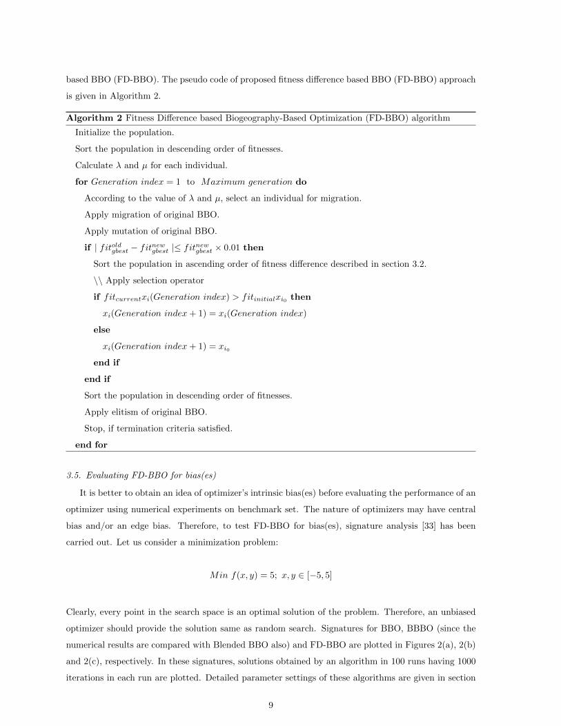
3.5. Evaluating FD-BBO for bias(es)
It is better to obtain an idea of optimizer’s intrinsic bias(es) before evaluating the performance of an
optimizer using numerical experiments on benchmark set. The nature of optimizers may have central
bias and/or an edge bias. Therefore, to test FD-BBO for bias(es), signature analysis [33] has been
carried out. Let us consider a minimization problem:
Min f(x, y) = 5; x, y ∈ [−5, 5]
Clearly, every point in the search space is an optimal solution of the problem. Therefore, an unbiased
optimizer should provide the solution same as random search. Signatures for BBO, BBBO (since the
numerical results are compared with Blended BBO also) and FD-BBO are plotted in Figures 2(a), 2(b)
and 2(c), respectively. In these signatures, solutions obtained by an algorithm in 100 runs having 1000
iterations in each run are plotted. Detailed parameter settings of these algorithms are given in section
9

3.6.
Let us define a solution (x, y) as an edge biased solution if
x ∈ [−5,−4] ∪ [4, 5] ∀y or
y ∈ [−5,−4] ∪ [4, 5] ∀x
and a center biased solution if x2 + y2 ≤ 1. It can be seen that the edge biased area covers 36% and
center biased area covers 3.14% of the total area in the search space. These areas are shown in Figure
3.
Table 1 shows the percentage of points which lies within the considered biased areas. It is clear that
BBBO is a center biased algorithm while BBO and proposed FD-BBO are almost un-biased algorithms.
That is the location of the optima will have the least impact on the performance of BBO and FD-BBO.
Figure 3: Edges bias and center bias areas
Table 1: Signature analysis
Biases Percentage of points by several algorithms
BBO BBBO FD-BBO
Central bias 3.02 43.78 3.80
Edge bias 41.78 1.84 37.80
3.6. Numerical experiments, discussion and statistical analysis of FD-BBO
In this paper, we considered a set of 15 unconstrained well-known benchmark problems. These 15
benchmarks are the collection of unimodal, multimodal and hybrid composite optimization problems.
For comparative study of several optimization procedures multidimensional (10 and 30- dimensional)
space are considered. These benchmark problems are given in Table 2 with their global optimum where
10

(a) Signature obtained from BBO algorithm
(b) Signature obtained from BBBO algorithm
(c) Signature obtained from FD-BBO algorithm
Figure 2: Signature of algorithms11

fmin is the optimum value of function and S ∈ RD is search space, where RD is Euclidean D-space (D
is dimension). More details of these benchmark functions are given in Suganthan et al. [34]. In Table
2, five test problems (f1, f2, f3, f4 and f5) are unimodal and remaining 10 test problems (f6 - f15) are
multimodal. Parameters setting for the numerical experiments is as follows:
Maximum immigration rate: I = 1
Maximum emigration rate : E = 1
Mutation probability = 0.01
Elitism size = 2
Population size = 50
Maximum number of iterations = 1000
Number of runs = 100
In this work, the stopping criteria are maximum number of generation and best absolute error (E) =
| f(X)− f(X∗) | ≤ θ, where f(X) is current best value of function, f(X∗) is the global optimum and
θ is an acceptable error for the function. The acceptable error θ of all the considered algorithms is set
to 10−6 for functions f1 to f5 and 10−2 for the remaining functions.
In Tables 3 and 4, we compare fitness difference based BBO (FD-BBO) with BBO and advanced version
of BBO, blended BBO (BBBO). Tables 3 and 4 represent the numerical results based on basic BBO,
BBBO and FD-BBO corresponding to 10 and 30-dimensional benchmark functions, respectively. Table
3 presents the minimum error (MinE), standard deviation (SD) and mean error (ME) of BBO, BBBO
and FD-BBO for 10-dimensional problems. Table 4 presents the same for 30-dimensional problems. In
Tables 3 and 4, bold entries represent the best results of the three algorithms. From these results, it
is clear that FD-BBO is a better optimizer based on the minimum error (MinE), standard deviation
(SD) and mean error (ME) for both considered dimensional (10 and 30-dimensional) space.
Table 2: Test problems [34](TP: Test problem, D: Dimension, S: Search space, fmin = Optimum)
TP Objective function S fmin
f1 Shifted sphere function [−100, 100]D -450
f2 Shifted Schwefels problem 1.2 [−100, 100]D -450
f3 Shifted rotated high conditional elliptic function [−100, 100]D -450
f4 Shifted Schwefels problem 1.2 with noise in fitness [−100, 100]D -450
f5 Schwefels problem 2.6 with global optimum on bounds [−100, 100]D -310
f6 Shifted Rosenbrocks function [−100, 100]D 390
f7 Shifted rotated Griewanks function without bounds No bounds -180
f8 Shifted rotated Ackleys function with global optimum on
bounds
[−32, 32]D -140
f9 Shifted Rastrigins function [−5, 5]D -330
f10 Shifted rotated Rastrigins function [−5, 5]D -330
f11 Shifted rotated Weierstrass function [−0.5, 0.5]D 90
f12 Schwefels problem 2.13 [π, π]D -460
f13 Expanded extended Griewanks plus Rosenbrocks function [−3, 1]D -130
f14 Shifted rotated expanded Scaffers [−100, 100]D -300
f15 Hybrid composite function [−5, 5]D 120
12

Table 3: Comparison of results of BBO, BBBO and FD-BBO for 10-dimensional problems (TP: Test problem, Min E =
Minimum error, SD = Standard deviation, ME = Mean error)
TP Algorithm Min E SD ME
f1 BBO 2.4617E-02 6.4588E-02 1.0041E-01
BBBO 7.6819E-04 2.5012E-02 2.6778E-02
FD-BBO 4.0935E-03 2.2137E-02 2.8049E-02
f2 BBO 1.4006E+01 1.1067E+02 1.1199E+02
BBBO 2.6916E+01 1.1713E+02 1.8285E+02
FD-BBO 5.8954E-01 2.6870E+00 6.3194E+00
f3 BBO 9.8673E+05 4.9524E+06 7.7719E+06
BBBO 1.0348E+06 3.4284E+06 6.0936E+06
FD-BBO 2.7731E+04 1.7557E+05 3.0033E+05
f4 BBO 4.7471E+01 5.9329E+02 5.2255E+02
BBBO 7.0507E+02 1.5748E+03 2.7125E+03
FD-BBO 9.1345E-01 7.1893E+01 9.1644E+01
f5 BBO 5.9503E+01 8.5931E+02 8.7892E+02
BBBO 1.2415E+03 1.4186E+03 3.4340E+03
FD-BBO 8.5954E+00 4.6115E+02 3.8738E+02
f6 BBO 1.2517E+01 2.2913E+02 2.1786E+02
BBBO 7.3792E+00 2.3380E+02 1.9822E+02
FD-BBO 1.8530E-01 1.5012E+02 9.5420E+01
f7 BBO 3.7687E+02 2.1641E+02 8.6715E+02
BBBO 3.7628E+02 2.4282E+02 8.9723E+02
FD-BBO 8.6161E+01 2.0974E+02 7.5524E+02
f8 BBO 2.0141E+01 7.2909E-02 2.0910E+01
BBBO 2.0200E+01 6.9727E-02 2.0792E+01
FD-BBO 2.1633E+00 7.2796E-02 2.0003E+01
f9 BBO 8.9149E-03 5.1345E-02 5.5177E-02
BBBO 3.0264E-03 1.2956E-02 1.6702E-02
FD-BBO 6.4574E-03 8.8787E-03 3.5889E-03
f10 BBO 4.0483E+00 1.1921E+01 2.8729E+01
BBBO 8.0610E+00 1.4846E+01 3.7100E+01
FD-BBO 5.9857E+00 1.0469E+01 2.0794E+01
f11 BBO 2.0851E+00 5.9410E-01 3.2491E+00
BBBO 1.8590E+00 5.6747E-01 3.1773E+00
FD-BBO 9.4410E-02 4.4792E-01 2.0012E+00
f12 BBO 2.5632E+04 4.9307E+04 9.0889E+04
13

BBBO 1.2272E+05 1.0961E+05 3.1746E+05
FD-BBO 1.5690E+04 4.3856E+04 8.6478E+04
f13 BBO 2.7865E-02 1.4534E-01 2.1992E-01
BBBO 1.2529E-01 2.8279E-01 4.6183E-01
FD-BBO 4.8146E-03 1.6039E-01 2.1897E-01
f14 BBO 3.2650E+00 2.5751E-01 3.8253E+00
BBBO 2.9269E+00 3.0891E-01 3.7427E+00
FD-BBO 8.4217E-01 3.3399E-01 3.5728E+00
f15 BBO 1.5435E-01 2.1332E+02 3.8426E+02
BBBO 3.1769E-02 2.4464E+02 3.7389E+02
FD-BBO 4.6201E-02 2.1548E+02 9.1573E+01
Table 4: Comparison of results of BBO, BBBO and FD-BBO for 30-dimensional problems(TP: Test problem, Min E =
Minimum error, SD = Standard deviation, ME = Mean error)
TP Algorithm Min E SD ME
f1 BBO 1.6573E+00 1.5831E+00 4.1947E+00
BBBO 1.8028E+01 1.8912E+01 4.1695E+01
FD-BBO 3.9282E-01 4.2761E-01 1.2902E+00
f2 BBO 3.3139E+03 4.2894E+03 1.1059E+04
BBBO 3.9740E+03 1.6836E+03 6.7517E+03
FD-BBO 2.9032E+03 3.6948E+02 9.0165E+02
f3 BBO 1.4449E+07 1.9453E+07 5.1113E+07
BBBO 9.9106E+06 8.6095E+06 2.4715E+07
FD-BBO 1.2960E+07 1.0847E+07 3.1411E+07
f4 BBO 1.9067E+04 1.2022E+04 4.1006E+04
BBBO 1.2252E+04 4.7640E+03 2.1454E+04
FD-BBO 1.4162E+04 1.2864E+04 2.1373E+04
f5 BBO 6.1906E+03 3.0269E+03 1.1402E+04
BBBO 8.0081E+03 1.7290E+03 1.1190E+04
FD-BBO 1.8698E+03 1.5871E+03 1.1092E+04
f6 BBO 4.2721E+02 2.8497E+03 2.5133E+03
BBBO 1.1625E+04 4.8234E+04 7.1496E+04
FD-BBO 9.8158E+01 1.9333E+03 9.7674E+02
f7 BBO 2.1197E+03 4.4551E+02 3.0821E+03
BBBO 2.1714E+03 5.3827E+02 3.0941E+03
FD-BBO 1.0426E+03 3.0355E+02 3.0346E+03
f8 BBO 2.0934E+01 4.6289E-02 2.1030E+01
14

BBBO 2.0821E+01 7.3672E-02 2.0993E+01
FD-BBO 8.0855E-01 2.0429E-02 2.0010E+01
f9 BBO 5.3783E-01 6.2624E-01 1.5123E+00
BBBO 8.4677E+00 3.3147E+00 1.3725E+01
FD-BBO 3.1087E-02 2.0283E-01 5.6352E-01
f10 BBO 6.7278E+01 3.5308E+01 1.6737E+02
BBBO 1.0885E+02 3.3999E+01 1.9952E+02
FD-BBO 5.0775E+00 2.1368E+01 1.1031E+02
f11 BBO 1.3131E+01 1.5468E+00 1.9974E+01
BBBO 1.3752E+01 1.5462E+00 2.1888E+01
FD-BBO 1.0819E+00 1.1145E+00 1.5308E+01
f12 BBO 9.3288E+05 4.2107E+05 1.8936E+06
BBBO 1.5834E+06 7.1076E+05 2.9137E+06
FD-BBO 1.0290E+06 5.7236E+05 1.8513E+06
f13 BBO 5.1194E-01 3.9303E-01 1.5398E+00
BBBO 2.1945E+00 7.1228E-01 3.4904E+00
FD-BBO 6.5521E-02 2.2139E-02 1.1788E+00
f14 BBO 1.2659E+01 3.1689E-01 1.3393E+01
BBBO 1.2196E+01 4.5169E-01 1.3411E+01
FD-BBO 1.4462E-01 3.3923E-02 1.2488E+00
f15 BBO 2.2802E+02 1.8146E+02 4.2334E+02
BBBO 5.6373E+01 1.6156E+02 4.3050E+02
FD-BBO 6.5492E-01 9.4871E+01 2.5967E+02
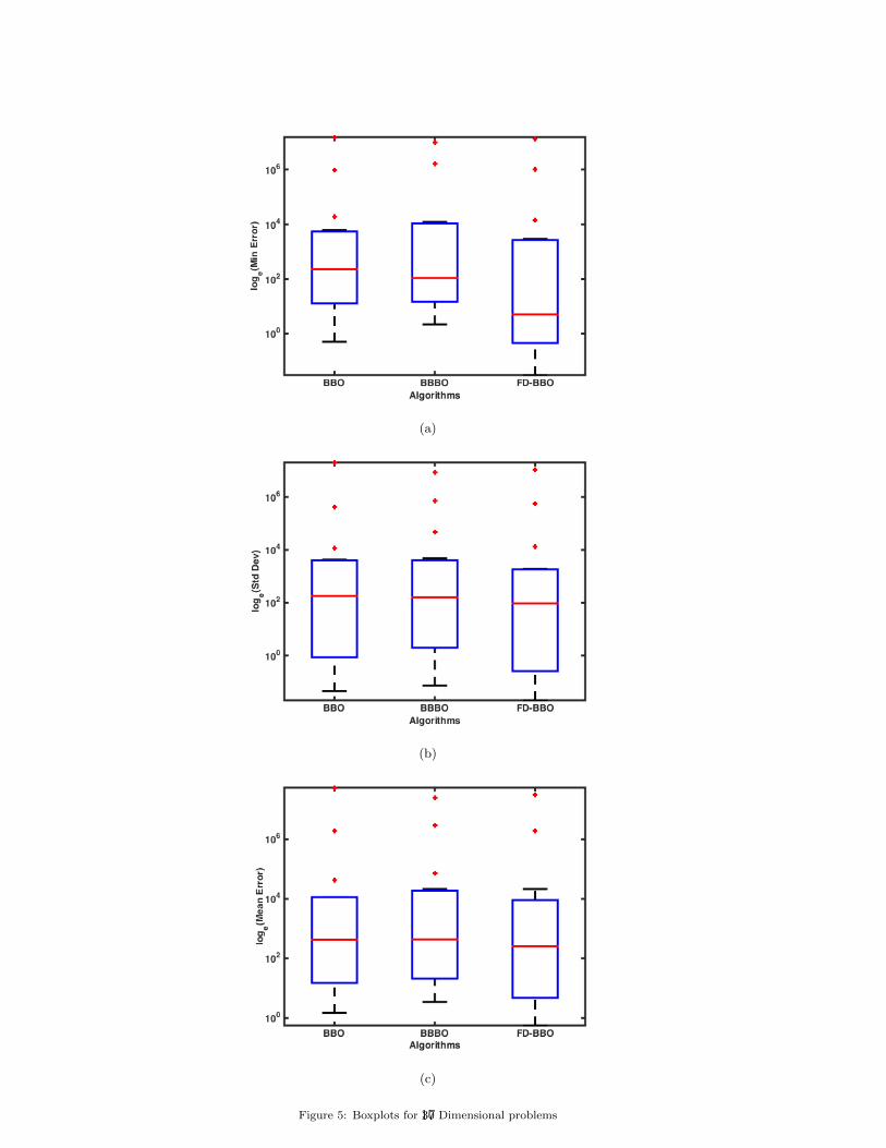
Some more intensive statistical analyses have been carried out with the numerical results of BBO,
BBBO and FD-BBO. The boxplots are the empirical distribution of data. Boxplots for minimum
error, standard deviation and mean error corresponding to all algorithms BBO, BBBO and FD-BBO
are given in Figures 4 and 5 for 10-dimensional and 30-dimensional problems, respectively. From the
boxplot analyses, FD-BBO performs better than other considered algorithms for 10 and 30-dimensional
problems. To see the significant difference between two algorithms among considered algorithms a
non-parametric test, Mann-Whitney U rank sum test is applied. The results of Mann-Whitney U rank
sum test for minimum error of 100 simulations are given in Table 5. In Table 5, ‘+’ sign appears
if FD-BBO is the better algorithm, ‘-’ sign appears if FD-BBO is the worse algorithm and ‘=’ sign
appears if FD-BBO is not significantly different than compared algorithms. There are 24 ‘+’ signs
out of 30 comparisons and 22 ‘+’ signs out of 30 comparisons in Table 5 for 10 and 30-dimensional
problems, respectively. Therefore, the conclusion from all analyses is that FD-BBO is significantly a
better optimizer than BBO and BBBO.
15

(a)
(b)
(c)
Figure 4: Boxplots for 10 Dimensional problems16
(a)
(b)
(c)
Figure 5: Boxplots for 30 Dimensional problems17

Table 5: Mann-Whitney U rank sum test (TP: Test Problem)
For 10-dimensional problems For-30 dimensional problems
TP FD-BBO Vs
BBO
FD-BBO Vs
BBBO
TP FD-BBO Vs
BBO
FD-BBO Vs
BBBO
f1 = = f1 = +
f2 + + f2 + +
f3 + + f3 + -
f4 + + f4 + +
f5 + + f5 + +
f6 + = f6 + +
f7 + + f7 + +
f8 + + f8 = =
f9 + + f9 + +
f10 + + f10 + +
f11 + + f11 + +
f12 + + f12 + +
f13 = + f13 = =
f14 = = f14 = =
f15 + + f15 + +
Total number
of ‘+’ signs
12 12 Total number
of ‘+’ signs
11 11
4. Wind farm layout problem formulation
4.1. Wind farm model
There are some assumptions in wind farm modeling. The wake model in this study is considered
from N. O. Jenson model [5, 35]. In this wake model momentum is conserved. The downstream wind
speed in jth turbine under the influence of ith turbine is calculated by
uj = u0j
[1− 2a
(1 + αidijr′i
)2
](9)
a =1−
√(1− CT )
2(10)
r′i = ri
√(1− a1− 2a
)(11)
αi =0.5
ln(hi
z0)
(12)
Where, u0j is the free stream wind speed at jth turbine
a is the axial induction factor
dij is the distance between ith and jth turbine
ri is the rotor radius of ith turbine
r′i is the downstream rotor radius of ith turbine
hi is the hub height of ith turbine
CT is the thrust coefficient of the wind turbine, which is considered same for all turbines
αi is the entrainment constant pertaining to ith turbine
18

z0 is the surface roughness of wind farm
The wake region is conical for the linear wake model and radius of the wake region is represented by
wake influence radius which is defined as:
Rwi = αidij + r′i (13)
A linear wake model of jth turbine under the influence of ith turbine is shown in Figure 6.
Figure 6: Linear wake model of wind turbine
At an instant any wind turbine is under the multiple wake region, i.e. wind turbines’ velocity is
influenced by multiple wakes. The wind speed of ith turbine is calculated using the assumption that
kinetic energy deficit of the mixed wake is equal to the sum of the energy deficits as follows:
uk = u0k
[1−
√√√√ NT∑m=1
(1− ukm
u0m
)2]
(14)
Where u0k and u0m are free stream wind velocity without wake effect at kth and mth turbine, respec-
tively. ukm is the wind velocity at kth turbine under the wake region of mth turbine. NT is the total
number of turbines influencing the kth turbine with wake effect.
Here we have considered a constant wind speed and fixed wind direction (south to north). Total power
output for each turbine in one year is calculated as:
Pi = 0.5 ∗ ρ ∗ π ∗ r2i ∗ u3
i ∗Cp
1000kW, i = 1, 2, ...., NT (15)
19

Where ρ represents the air density and Cp represents the rotor efficiency.
The total power generated by wind farm in one year is calculated as:
Ptotal =
NT∑i=1
Pi (16)
We considered Mosetti’s cost model having NT number of turbines as:
Cost = NT
(2
3+
1
3exp−0.00174N2
T
)(17)
In this study, turbines’ position are intersection points of the grid within the wind farm. We are not
considering the boundary of the wind farm as the potential location for turbines.
The main objective of the study is highest power output at minimum cost and can be formulated as:
Objective =Cost
Ptotal(18)
4.2. FD-BBO for wind farm layout optimization problem
In the literature, many non-conventional techniques, e.g. genetic algorithm (GA), Monte Carlo
simulation, Greedy algorithm, BBO, Cuckoo search etc. have been applied to solve wind farm layout
optimization problem. In the earlier studies, researchers have tried to find the optimal placement of
wind turbines so that power generation of wind farm maximizes. Now a days researchers are dealing to
find out the optimal configuration of wind turbines such as hub height and rotor radius along with the
optimal location of wind turbines. The results are motivating as compared to earlier studies. Therefore,
fitness difference based BBO approach is explored to find wind farm layout with optimal configurations
(hub heights and rotor radii) of wind turbines.
We considered a square wind farm of size 2000m × 2000m. The wind farm is subdivided into 100
grids each of size 200m × 200m. If we consider NT number of turbines whose hub heights and rotor
radii are not necessarily to be uniform to be placed, then any arrangement of these NT turbines in
a two-dimensional wind farm with several hub heights and rotor radii represent a potential solution
in FD-BBO. Thus ith solution is represented by (xti, yti , h
ti, r
ti). Where (xti, y
ti) is the position of tth
turbine while hti and rti are the hub height and rotor radius of tth turbine, respectively. Clearly, the
number of decision variables in this problem are 4NT . The step by step procedure to solve wind farm
layout and configuration problem by FD-BBO is given in Algorithm 3.
20

Algorithm 3 FD-BBO for wind farm layout optimization
Initialize the solution (habitat) (xti, yti , h
ti, r
ti), t = 1, 2, .....,NT ; i = 1, 2, ....., Np.
Compute ut, Pt and Ptotal using equations 14, 15 and 16.
Calculate λ and µ using equations 4 and 5.
Sort the population to decreasing order of total power output (Ptotal) of the wind farm.
for Generation index = 1 to Maximum generation do
According to the value of λ and µ, select habitat for migration.
Apply migration as in Algorithm 1.
Apply mutation as in Algorithm 1.
if | Ptotaloldgbest − Ptotalnewgbest |≤ Ptotal
newgbest × 0.01 then
Apply fitness difference based sorting strategy described in section 3.2.
end if
Compute ut, Pt and Ptotal for updated solutions.
Sort the population to decreasing order of total power output (Ptotal) of the wind farm.
Keep the elite solution.
Stop, if termination criteria satisfied.
end for
4.3. Results and discussion
For the considered square wind farm of size 2000m × 2000m, air density (ρ) is 1.2254 kg/m3, rotor
efficiency (Cp) is 0.4, thrust coefficient (CT ) is 8/9 and the surface roughness of wind farm (z0) is
0.3m. FD-BBO, BBO and BBBO are applied to solve wind farm layout optimization problem. The
parameters of these algorithms are same as in section 3.6.
In Table 6, the comparison between Mosetti et al.’s [1] results and present study results are carried out.
Results are compared for 26 number of turbines. In the Mosetti et al.’s study, hub height (h = 60m),
rotor radius (r = 20m) and thrust coefficient (CT = 0.88) were fixed for each turbine. In the present
study, we are also dealing to tune hub heights and rotor radii along with the optimal layout of wind
turbines. Total power output obtained in the present study is better than that of Mosetti et al. [1]
study. BBO and FD-BBO algorithms are performing better than earlier study, but FD-BBO algorithm
outperforms. Table 7 presents the comparison between Grady et al. [2] results and present study’s
results. Results are reported for 30 number of turbines. In Grady et al. [2] study, hub height, rotor
radius and thrust coefficient are same as given in Mosetti et al. [1]. In this comparison, total power
output obtained by BBO and FD-BBO is better than Grady et al. approach.
Figures 7 and 8, represent the optimal configuration of wind turbines. Figure 7(a) is the optimal
positions of 26 wind turbines given by Mosetti et al. [1] and Figures 7(b), 7(c) and 7(d) are optimal
position of 26 wind turbines by BBO, BBBO and FD-BBO algorithms, respectively. Figure 8(a) presents
the optimal position of 30 wind turbine obtained by Grady’s approach. Figures 8(b), 8(c) and 8(d)
21

Table 6: Comparison of present study results with Mosetti et al. [1] results
Parameters Mosetti [1] study Present study
Reported Calculated (With-
out Approximation)
Using
BBO
Using
BBBO
Using
FD-BBO
Number of turbine 26 26 26 26 26
Total power (kw year) 12352 12654 13653 12307 13683
Fitness value 0.0016197 0.001581 0.0014654 0.00162562 0.0014621
Table 7: Comparison of present study results with Grady et al. [2] results
Parameters Grady [2] study Present study
Reported Calculated (With-
out Approximation)
Using
BBO
Using
BBBO
Using
FD-BBO
Number of turbine 30 30 30 30 30
Total power (kw year) 14310 14667 15655 14090 15662
Fitness value 0.0015436 0.0015061 0.001411 0.00156769 0.0014103
present the optimal position of 30 wind turbines by BBO, BBBO and FD-BBO algorithms, respectively.
The corresponding hub heights and rotor radii along with position coordinates obtained by BBO, BBBO
and FD-BBO approaches for 26 and 30 wind turbines are presented in Tables 8 and 9, respectively.
22

(a) By Mosetti et al. using GA (b) By present study using BBO
(c) By present study using BBBO (d) By present study using FD-BBO
Figure 7: Optimal configurations of 26 wind turbines
23

(a) By Grady et al. using GA (b) By present study using BBO
(c) By present study using BBBO (d) By present study using FD-BBO
Figure 8: Optimal configurations of 30 wind turbines
24

Table 8: 26 wind turbines positions, hub heights and rotor radii obtained by BBO, BBBO and FD-BBO in a 2000m × 2000m square farm
Using BBO Using BBBO Using FD-BBO
Optimal posi-
tion
Rotor ra-
dius
Hub
height
Optimal posi-
tion
Rotor ra-
dius
Hub
height
Optimal posi-
tion
Rotor ra-
dius
Hub
height
(600, 1800)19.9647 51.7587 (400, 1000) 19.7091 32.7375 (1600, 1600) 19.8535 44.1743
(600, 1600) 19.8356 33.3044 (1000, 1200) 18.1712 47.4873 (1200, 1400) 19.9369 31.6778
(1800, 1800) 19.9471 25.3969 (1600, 1800) 19.5334 22.9533 (600, 1400) 19.9466 46.6166
(200, 1600) 19.7876 42.0720 (600, 1600) 17.2568 30.6825 (1400, 1200) 19.9668 37.3379
(600, 1400) 19.9381 34.0635 (200, 1600) 18.5133 22.6059 (1600, 1200) 19.9485 42.4154
(1000, 1800) 19.8236 43.1484 (600, 1400) 18.1056 28.4428 (400, 800) 19.7576 33.8037
(1000, 1600) 19.9443 41.0037 (600, 1000) 17.3077 25.8279 (1600, 1000) 19.9701 48.2209
(1400, 1800) 19.6782 20.5167 (400, 400) 18.9681 32.3002 (600, 400) 19.7962 34.7141
(1000, 800) 19.8934 47.2696 (800, 1600) 18.5899 54.1832 (200, 1800) 19.8521 46.0036
(800, 1600) 19.5185 53.0970 (600, 400) 19.6350 51.2949 (400, 600) 19.9661 35.3177
(800, 400) 19.9536 39.7455 (1400, 1800) 18.6810 49.9452 (200, 600) 19.9169 40.1456
(1200, 1000) 19.9330 32.9198 (1800, 1800) 19.6675 40.5307 (1600, 400) 19.9015 52.7761
(200, 800) 19.9656 27.6139 (1800, 1600) 18.6534 53.9258 (1000, 1800) 19.9519 36.4000
(800, 200) 19.8181 21.2555 (1000, 600) 18.7560 55.5234 (1000, 600) 19.6389 21.6649
(1800, 1600) 19.8929 42.6978 (1400, 1200) 19.9923 59.7716 (1400, 600) 19.8843 31.7090
(1000, 600) 19.9764 32.9999 (1200, 600) 19.5760 22.8167 (800, 1800) 19.6078 21.0827
(1600, 1400) 19.8703 31.6229 (1200, 400) 18.9420 44.3078 (800, 1000) 19.8852 43.0994
(1800, 400) 19.9220 57.2311 (1800, 1000) 18.4184 20.3368 (400, 400) 19.9487 37.7021
(400, 600) 19.9988 51.5441 (1400, 800) 18.1485 40.9401 (800, 800) 19.7267 47.7567
(1200, 800) 19.9734 23.4229 (200, 1400) 19.5030 33.3717 (1000, 400) 19.9772 59.8607
(600, 200) 19.6576 47.3918 (800, 1200) 19.5509 42.7233 (600, 200) 19.9696 43.4479
(1400, 600) 19.6436 26.6658 (1600, 1400) 17.9891 29.9358 (200, 400) 19.9387 38.6388
(1200, 400) 19.9544 57.3936 (1000, 400) 18.9600 49.8480 (1200, 200) 19.9450 55.3500
25

(1200, 200) 19.7656 43.7386 (1600, 600) 19.8247 51.0533 (800, 200) 19.9233 44.1171
(1600, 400) 19.8683 30.2834 (1800, 400) 19.4638 35.5381 (1600, 200) 19.9372 44.2013
(200, 200) 19.9936 56.3159 (800, 800) 18.1130 37.9484 (1000, 200) 19.9414 28.0759
26

Table 9: 30 wind turbines positions, hub heights and rotor radii obtained by BBO, BBBO and FD-BBO in a 2000m × 2000m square farm
Using BBO Using BBBO Using FD-BBO
Optimal posi-
tion
Rotor ra-
dius
Hub
height
Optimal posi-
tion
Rotor ra-
dius
Hub
height
Optimal posi-
tion
Rotor ra-
dius
Hub
height
(600, 1800)19.9794 49.2502 (1000, 1800) 18.4216 44.5251 (600, 1800) 19.4316 29.4083
(200, 1800) 19.9533 47.0476 (800, 1600) 18.8931 37.8571 (1800, 1800) 19.9252 49.6617
(1200, 1800) 19.9521 27.8465 (1400, 1400) 18.8165 57.4066 (600, 800) 19.9679 50.2845
(400, 1800) 19.9832 37.4665 (1200, 1800) 17.3464 53.0912 (800, 1600) 19.9843 29.9192
(1000, 1600) 19.7984 56.7558 (600, 1600) 18.9351 22.4174 (1800, 1600) 19.8893 53.4238
(1800, 1000) 19.8607 58.2722 (800, 1200) 19.5773 55.1218 (600, 400) 19.7590 39.1783
(1600, 1200) 19.8335 50.4844 (800, 800) 19.1297 51.5130 (1400, 1800) 19.9329 25.1884
(200, 600) 19.1115 58.6931 (600, 1200) 18.8977 38.6689 (1000, 1800) 19.9310 49.7733
(1000, 1000) 19.9443 38.8130 (600, 800) 19.2367 51.7145 (800, 400) 19.9947 57.7767
(1600, 600) 19.8536 58.1634 (200, 800) 19.5784 42.4235 (400, 1400) 19.8710 30.3715
(600, 1200) 19.5502 50.7616 (1200, 1400) 19.1018 50.5052 (1400, 1600) 19.8973 32.8607
(600, 600) 19.7520 33.4019 (1000, 600) 19.8819 29.5753 (400, 400) 19.6900 39.9654
(1800, 800) 19.8077 26.6128 (600, 400) 18.9865 54.3138 (200, 1800) 19.6931 50.0896
(1400, 1200) 19.7821 42.7594 (1000, 400) 19.4693 43.5557 (1800, 1000) 19.8026 55.7636
(600, 400) 19.9456 24.4669 (800, 200) 18.6991 55.7785 (200, 600) 19.7797 51.3783
(400, 600) 19.6468 42.4717 (1600, 1600) 19.8078 58.1218 (200, 400) 19.7526 45.5725
(1400, 1000) 19.9953 28.4426 (400, 800) 18.8033 28.4088 (1000, 1600) 19.9535 58.7362
(1600, 200) 19.7998 26.6100 (600, 200) 19.7916 33.5676 (400, 200) 19.6580 33.8476
(200, 400) 19.9044 33.4797 (1000, 200) 18.8068 20.9897 (1200, 800) 19.6410 47.6596
(1000, 600) 19.7792 47.2829 (1400, 1000) 17.1594 29.2716 (1400, 800) 19.9477 55.6132
(200, 200) 19.9654 45.4332 (1800, 1600) 17.8168 36.6510 (800, 200) 19.8440 26.8447
(1200, 200) 19.7980 58.8234 (1200, 1000) 19.5788 53.3900 (1600, 1200) 19.9954 54.4604
(1000, 200) 19.8976 35.8667 (1200, 600) 14.5978 34.3058 (1600, 1000) 19.7439 53.0715
27

(1400, 600) 19.9817 22.5718 (1600, 1400) 19.7690 39.1186 (1400, 200) 19.9998 22.5858
(800, 1200) 19.7910 36.9339 (1600, 1200) 17.7152 51.7474 (1600, 600) 19.9601 44.5301
(400, 400) 19.9749 34.4737 (1600, 1000) 18.3185 55.6551 (1000, 1000) 19.6361 47.8160
(1800, 200) 19.8868 47.4931 (1800, 1200) 19.5529 56.4666 (1800, 800) 19.2492 20.1137
(400, 200) 19.3745 19.8123 (1800, 200) 17.6082 25.6741 (1600, 200) 19.8545 46.0326
(1400, 200) 19.9383 56.3447 (400, 200) 18.6487 48.2097 (1000, 400) 19.7053 53.1190
(800, 200) 19.2541 28.0815 (1600, 600) 19.7819 58.0076 (1800, 600) 19.7639 39.1860
28

From the observation of results reported in Tables 8 and 9, there are variations of hub heights and
rotor radii in wind turbines. Practically, many variants of rotor radii and hub heights as the number of
turbines are not possible. For practical purpose three different rotor radii and hub heights are selected for
both the cases from Tables 8 and 9. For 26 wind turbines three rotor radii (R1 = 19.8934, R2 = 18.9420
and R3 = 19.9369) and three hub heights (H1 = 39.7455, H2 = 40.5307 and H3 = 42.4154) are
selected from Table 8. These selected rotor radii R1, R2 and R3 are the median of columns 2, 5 and 8,
respectively. Observed hub heights H1, H2 and H3 are the median of columns 3, 6 and 9, respectively.
In case of 30-wind turbines, three rotor radii and three hub heights are selected from Table 9 through the
same observation. Here three different rotor radii (R′1 = 19.8571, R′2 = 18.9164 and R′3 = 19.8492) and
three different hub heights (H ′1 = 40.6423, H ′2 = 46.3674 and H ′3 = 46.8461) are observed. Considered
rotor radii R′1, R′2 and R′3 are the median of columns 2, 5 and 8, respectively as well as three hub
heights H ′1, H ′2 and H ′3 are the median of columns 3, 6 and 9, respectively.
Again optimal position of wind turbines are reproduced from observed set of rotor radii and hub heights
for both cases. The increased total power output of wind farm for both the cases are reported in Tables
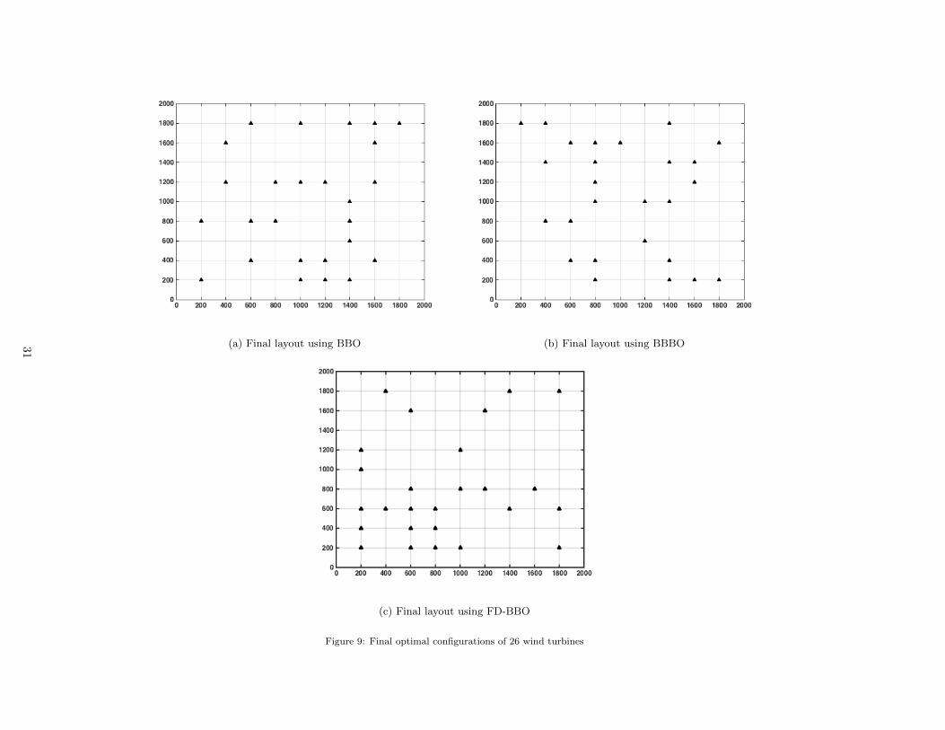
10 and 11. Thus the optimal layout corresponding to given Tables 10 and 11 are represented in Figures 9
and 10, respectively. In Figure 9, we can see the final optimal configuration of 26-wind turbines achieved
by three techniques. Figures 9(a), 9(b) and 9(c) represent the optimal layout of wind turbines using
BBO, BBBO and FD-BBO, respectively. In Figure 9(a) and 9(b), all 26-wind turbines have different
three choices of rotor radii (R1, R2, R3 ) as well as hub heights (H1, H2, H3). But in Figure 9(c), all wind
turbines have unique rotor radius (R3) along with the variation of hub heights (H1, H2, H3). Similarly,
in Figure 10, the final optimal configuration of 30-wind turbines are given which is again achieved by
three techniques. Figures 10(a), 10(b) and 10(c), represent the optimal layout of wind turbines using
BBO, BBBO and FD-BBO, respectively. Here in Figures 10(a) and 10(b), all 30-wind turbines have
different choices of rotor radii (R′1, R′2, R′3) as well as hub heights (H ′1, H ′2, H ′3). In Figure 10(c),
corresponding to several hub heights (H ′1, H ′2, H ′3) there is one rotor radius (R′1) is obtained by FD-
BBO. Therefore, FD-BBO is considered a good optimizer to find the optimal rotor radii (R3) and (R′1)
corresponding to the cases 26-wind turbines and 30-wind turbines, respectively.
The corresponding position co-ordinates of 26-wind turbines along with hub heights and rotor radii using
considered algorithms are given in Table 12. In case of 26-wind turbines, it is observed from the above
discussion that FD-BBO gives the promising solution by selecting best rotor radius (R3 = 19.9369)
from the given rotor radii (R1, R2 and R3). The recommended rotor radius R3 is the median of rotor
radii obtained by FD-BBO. The obtained energy production reported in Tables 10 shows that FD-BBO
outperforms over BBO and BBBO. Again the same analysis is done for 30-wind turbines. Here in Table
13, the corresponding position co-ordinates along with hub heights and rotor radii using considered
algorithms are given. Again FD-BBO outperforms over BBO and BBBO by selecting the best rotor
radius (R′1 = 19.8571) among the given set of rotor radii (R′1, R′2 and R′3).
Through these analysis of the results for both the cases (26-wind turbines and 30-wind turbines) given
29

in Tables 10, 11, 12 and 13, FD-BBO is recommended a good optimizer to find the optimal configuration
of wind turbines. In both the cases, FD-BBO recommends the best rotor radius from the given set
of rotor radii. Also FD-BBO is able to find the best optimal placement of wind turbines along with
suitable hub heights. The above discussion clearly shows the performance of FD-BBO is better than
BBO and blended BBO. FD-BBO is able to find the best rotor radius which is most convenient and
reliable to constructing the promising wind farm. Therefore, FD-BBO is better optimizer for selecting
most appropriate rotor radius along with suitable hub height to produce the maximum energy.
Table 10: Final energy output of wind farm for case 1
Parameter Using BBO Using BBBO Using FD-BBO
Number of turbine 26 26 26
Total power (kw
year)
13745 13620 13750
Fitness value 0.00145550 0.00146888 0.00145510
Table 11: Final energy output of wind farm for case 2
Parameter Using BBO Using BBBO Using FD-BBO
Number of turbine 30 30 30
Total power (kw
year)
15736 15460 15738
Fitness value 0.00140374 0.00142874 0.00140352
30
(a) Final layout using BBO (b) Final layout using BBBO
(c) Final layout using FD-BBO
Figure 9: Final optimal configurations of 26 wind turbines
31

(a) Final layout using BBO (b) Final layout using BBBO
(c) Final layout using FD-BBO
Figure 10: Final optimal configurations of 30 wind turbines
32

Table 12: Final 26 wind turbines positions, hub heights and rotor radii obtained by BBO, BBBO and FD-BBO in a 2000m × 2000m square farm
Using BBO Using BBBO Using FD-BBO
Optimal posi-
tion
Rotor ra-
dius
Hub
height
Optimal posi-
tion
Rotor ra-
dius
Hub
height
Optimal posi-
tion
Rotor ra-
dius
Hub
height
(1000, 1800)19.9369 40.5307 (1400, 1800) 19.9369 40.5307 (400, 1800) 19.9369 42.4154
(1400, 1800) 19.9369 39.7455 (600, 1600) 19.9369 40.5307 (600, 1600) 19.9369 40.5307
(1200, 1200) 19.8934 42.4154 (1400, 1400) 19.9369 40.5307 (600, 800) 19.9369 42.4154
(1400, 1000) 19.9369 40.5307 (800, 1400) 19.8934 42.4154 (1000, 1200) 19.9369 40.5307
(1200, 400) 19.9369 42.4154 (600, 800) 19.8934 40.5307 (1200, 1600) 19.9369 40.5307
(800, 1200) 19.9369 42.4154 (800, 1200) 19.9369 40.5307 (600, 600) 19.9369 40.5307
(400, 1600) 19.9369 42.4154 (1400, 1000) 19.8934 42.4154 (1000, 800) 19.9369 40.5307
(1800, 1800) 19.9369 42.4154 (600, 400) 19.8934 42.4154 (1800, 1800) 19.9369 39.7455
(600, 1800) 19.9369 40.5307 (1400, 400) 19.9369 40.5307 (1200, 800) 19.9369 42.4154
(1600, 1800) 19.9369 42.4154 (800, 1000) 19.8934 40.5307 (1800, 600) 19.9369 40.5307
(600, 800) 19.9369 39.7455 (1200, 1000) 19.9369 39.7455 (600, 400) 19.9369 42.4154
(1000, 1200) 19.8934 42.4154 (400, 1800) 19.9369 42.4154 (800, 600) 19.9369 40.5307
(1000, 400) 19.9369 40.5307 (1600, 1400) 19.8934 40.5307 (1800, 200) 19.9369 40.5307
(800, 800) 19.9369 42.4154 (400, 1400) 19.9369 40.5307 (1400, 1800) 19.9369 40.5307
(1400, 800) 19.9369 40.5307 (1800, 200) 19.9369 39.7455 (400, 600) 19.9369 40.5307
(200, 800) 19.9369 39.7455 (800, 400) 19.9369 39.7455 (600, 200) 19.9369 40.5307
(600, 400) 19.9369 40.5307 (1400, 200) 19.9369 40.5307 (1600, 800) 19.9369 40.5307
(1200, 200) 19.9369 42.4154 (1800, 1600) 19.9369 42.4154 (200, 1200) 19.9369 40.5307
(400, 1200) 19.9369 42.4154 (400, 800) 19.9369 42.4154 (200, 1000) 19.9369 39.7455
(200, 200) 19.9369 42.4154 (200, 1800) 19.9369 40.5307 (800, 400) 19.9369 40.5307
(1400, 600) 19.9369 42.4154 (1600, 1200) 19.9369 40.5307 (1000, 200) 19.9369 40.5307
(1600, 1600) 19.9369 40.5307 (800, 1600) 19.9369 40.5307 (200, 600) 19.9369 40.5307
(1000, 200) 19.9369 40.5307 (1600, 200) 19.9369 39.7455 (200, 400) 19.9369 40.5307
33

(1400, 200) 19.9369 42.4154 (1000, 1600) 19.9369 40.5307 (1400, 600) 19.9369 40.5307
(1600, 1200) 19.9369 39.7455 (800, 200) 18.942 40.5307 (200, 200) 19.9369 40.5307
(1600, 400) 19.9369 39.7455 (1200, 600) 19.9369 40.5307 (800, 200) 19.9369 42.4154
34

Table 13: Final 30 wind turbines positions, hub heights and rotor radii obtained by BBO, BBBO and FD-BBO in a 2000m × 2000m square farm
Using BBO Using BBBO Using FD-BBO
Optimal posi-
tion
Rotor ra-
dius
Hub
height
Optimal posi-
tion
Rotor ra-
dius
Hub
height
Optimal posi-
tion
Rotor ra-
dius
Hub
height
(1800, 1600)19.8571 39.6423 (1800, 1800) 19.8571 39.6423 (1800, 1600) 19.8571 39.6423
(200, 1600) 19.8492 46.8961 (600, 1600) 19.8492 46.8961 (400, 1800) 19.8571 46.3674
(1000, 1400) 19.8571 39.6423 (1000, 1600) 19.8492 46.8961 (1600, 1800) 19.8571 39.6423
(1800, 800) 19.8571 46.3674 (1800, 800) 19.8571 46.3674 (600, 1200) 19.8571 46.3674
(400, 1400) 19.8492 46.3674 (400, 1400) 19.8492 46.3674 (400, 1000) 19.8571 46.3674
(1400, 1800) 19.8571 46.8961 (1400, 1800) 19.8571 46.8961 (1600, 1600) 19.8571 46.8961
(1600, 1600) 19.8571 46.3674 (1600, 1600) 19.8492 46.8961 (1400, 1200) 19.8571 46.3674
(1600, 1200) 19.8492 46.3674 (1600, 1200) 19.8492 46.3674 (1600, 1000) 19.8571 46.3674
(800, 1400) 19.8571 39.6423 (800, 1800) 19.8492 39.6423 (1000, 1200) 19.8571 39.6423
(400, 800) 19.8571 46.3674 (400, 800) 19.8571 46.3674 (1800, 1000) 19.8571 46.8961
(800, 600) 19.8571 39.6423 (800, 1200) 19.8571 39.6423 (1000, 800) 19.8571 39.6423
(200, 400) 19.8571 39.6423 (200, 1400) 19.8571 46.8961 (1800, 400) 19.8571 46.3674
(600, 1400) 19.8571 46.3674 (600, 1400) 19.8571 46.3674 (1800, 200) 19.8571 39.6423
(1000, 1000) 19.8571 46.8961 (1000, 1400) 19.8492 39.6423 (1000, 600) 19.8571 46.3674
(1000, 800) 19.8571 46.3674 (1000, 1200) 19.8571 46.3674 (800, 800) 19.8571 39.6423
(1600, 1000) 19.8571 46.3674 (1600, 1000) 19.8571 39.6423 (1600, 600) 19.8571 46.3674
(1800, 600) 19.8492 39.6423 (1800, 400) 18.9164 46.3674 (800, 600) 19.8571 46.3674
(600, 1000) 19.8571 46.3674 (600, 800) 19.8571 46.3674 (600, 600) 19.8571 46.3674
(1600, 600) 19.8571 46.3674 (1600, 1800) 19.8571 46.3674 (800, 400) 19.8571 46.8961
(1400, 1000) 19.8571 46.8961 (1400, 1000) 19.8492 46.3674 (1400, 1000) 19.8571 46.8961
(600, 400) 19.8571 39.6423 (1200, 400) 19.8571 39.6423 (1000, 400) 19.8571 46.3674
(600, 200) 19.8571 46.8961 (600, 1800) 19.8571 46.3674 (600, 200) 19.8571 46.3674
(1200, 1800) 19.8492 39.6423 (1200, 1800) 19.8492 39.6423 (1200, 1800) 19.8571 46.3674
35

(1600, 400) 19.8492 46.3674 (1600, 400) 19.8492 46.3674 (400, 400) 19.8571 46.3674
(1400, 800) 19.8571 39.6423 (1400, 800) 19.8571 39.6423 (1600, 200) 19.8571 46.3674
(1200, 1600) 19.8571 46.3674 (1200, 1600) 19.8571 46.8961 (1200, 1600) 19.8571 46.8961
(1800, 400) 19.8571 46.8961 (1200, 1400) 19.8571 46.8961 (200, 200) 19.8571 39.6423
(1200, 1200) 19.8571 39.6423 (1200, 200) 19.8571 39.6423 (1200, 1400) 19.8571 39.6423
(1400, 400) 19.8571 39.6423 (1400, 400) 19.8571 39.6423 (1200, 400) 19.8571 39.6423
(400, 600) 19.8571 46.3674 (400, 200) 19.8571 46.3674 (800, 200) 19.8571 39.6423
36

5. Conclusion
The paper proposes an improvement in biogeography based optimization (BBO) based on fitness
difference strategy (FD-BBO) and its application in solving the wind farm layout optimization problem
with non-uniform hub height and rotor radius. The proposed FD-BBO is shown to be an efficient
optimization algorithm by numerical experiments on benchmark test problems. A square wind farm
of 2000m × 2000m is taken for numerical experiments of wind farm layout optimization problem.
Two cases with 26 turbines and 30 turbines are considered for the experiments. Obtained results are
compared with earlier published results and the results obtained by basic BBO and blended BBO.
FD-BBO outperforms over all for both the cases. For each case, FD-BBO recommended the single
rotor radius which decreases the manufacturer cost of the wind farm. Thus FD-BBO is recommended
as reliable and a potential algorithm to solve wind farm layout optimization problem.
6. Acknowledgment
The second author acknowledges the funding from South Asian University, New Delhi, India to carry
out this research.
[1] G. Mosetti, C. Poloni, B. Diviacco, Optimization of wind turbine positioning in large windfarms
by means of a genetic algorithm, Journal of Wind Engineering and Industrial Aerodynamics 51 (1)
(1994) 105–116.
[2] S. Grady, M. Hussaini, M. M. Abdullah, Placement of wind turbines using genetic algorithms,
Renewable energy 30 (2) (2005) 259–270.
[3] G. Marmidis, S. Lazarou, E. Pyrgioti, Optimal placement of wind turbines in a wind park using
monte carlo simulation, Renewable energy 33 (7) (2008) 1455–1460.
[4] J.-F. Herbert-Acero, J.-R. Franco-Acevedo, M. Valenzuela-Rendon, O. Probst-Oleszewski, Lin-
ear wind farm layout optimization through computational intelligence, in: Mexican International
Conference on Artificial Intelligence, Springer, 2009, pp. 692–703.
[5] N. O. Jensen, A note on wind generator interaction, 1983.
[6] A. Mittal, Optimization of the layout of large wind farms using a genetic algorithm, Ph.D. thesis,
Case Western Reserve University (2010).
[7] J. S. Gonzalez, A. G. G. Rodriguez, J. C. Mora, J. R. Santos, M. B. Payan, Optimization of wind
farm turbines layout using an evolutive algorithm, Renewable energy 35 (8) (2010) 1671–1681.
[8] S. Chowdhury, J. Zhang, A. Messac, L. Castillo, Unrestricted wind farm layout optimization
(uwflo): Investigating key factors influencing the maximum power generation, Renewable Energy
38 (1) (2012) 16–30.
37

[9] Y. Chen, H. Li, K. Jin, Q. Song, Wind farm layout optimization using genetic algorithm with
different hub height wind turbines, Energy Conversion and Management 70 (2013) 56–65.
[10] J. Park, K. H. Law, Layout optimization for maximizing wind farm power production using se-
quential convex programming, Applied Energy 151 (2015) 320–334.
[11] K. Chen, M. Song, X. Zhang, S. Wang, Wind turbine layout optimization with multiple hub height
wind turbines using greedy algorithm, Renewable Energy 96 (2016) 676–686.
[12] J. C. Bansal, P. Farswan, Wind farm layout using biogeography based optimization, Renewable
Energy 107 (2017) 386–402.
[13] X.-S. Yang, S. Deb, Cuckoo search via levy flights, in: Nature & Biologically Inspired Computing,
2009. NaBIC 2009. World Congress on, IEEE, 2009, pp. 210–214.
[14] S. Rehman, S. Ali, S. Khan, Wind farm layout design using cuckoo search algorithms, Applied
Artificial Intelligence (2017) 1–24.
[15] A. Vasel-Be-Hagh, C. L. Archer, Wind farm hub height optimization, Applied Energy 195 (2017)
905–921.
[16] D. Simon, Biogeography-based optimization, Evolutionary Computation, IEEE Transactions on
12 (6) (2008) 702–713.
[17] H. Ma, D. Simon, Blended biogeography-based optimization for constrained optimization, Engi-
neering Applications of Artificial Intelligence 24 (3) (2011) 517–525.
[18] Q. Feng, S. Liu, J. Zhang, G. Yang, L. Yong, Biogeography-based optimization with improved
migration operator and self-adaptive clear duplicate operator, Applied Intelligence 41 (2) (2014)
563–581.
[19] G. Xiong, D. Shi, X. Duan, Enhancing the performance of biogeography-based optimization using
polyphyletic migration operator and orthogonal learning, Computers & Operations Research 41
(2014) 125–139.
[20] G.-G. Wang, A. H. Gandomi, A. H. Alavi, An effective krill herd algorithm with migration operator
in biogeography-based optimization, Applied Mathematical Modelling 38 (9) (2014) 2454–2462.
[21] P. Farswan, J. C. Bansal, Migration in biogeography-based optimization, in: Proceedings of Fourth
International Conference on Soft Computing for Problem Solving, Springer, 2015, pp. 385–397.
[22] P. Farswan, J. C. Bansal, K. Deep, A modified biogeography based optimization, in: 2nd Inter-
national Conference on Harmony Search Algorithm (ICHSA), Korea Univ, Seoul, South Korea:
Springer-Verlag Berlin, Springer, 2016, pp. 227–238.
38

[23] W. Guo, L. Wang, C. Si, Y. Zhang, H. Tian, J. Hu, Novel migration operators of biogeography-
based optimization and markov analysis, Soft Computing (2016) 1–28.
[24] M. Lohokare, S. S. Pattnaik, B. K. Panigrahi, S. Das, Accelerated biogeography-based optimization
with neighborhood search for optimization, Applied Soft Computing 13 (5) (2013) 2318–2342.
[25] J. C. Bansal, Modified blended migration and polynomial mutation in biogeography-based opti-
mization, Harmony Search Algorithm. Springer (2016) 217–225.
[26] D. Simon, M. G. Omran, M. Clerc, Linearized biogeography-based optimization with re-
initialization and local search, Information Sciences 267 (2014) 140–157.
[27] J. C. Bansal, P. Farswan, A novel disruption in biogeography-based optimization with application
to optimal power flow problem, Applied Intelligence (2016) 1–26.
[28] J. C. Bansal, H. Sharma, K. Arya, K. Deep, M. Pant, Self-adaptive artificial bee colony, Optimiza-
tion 63 (10) (2014) 1513–1532.
[29] J. C. Bansal, H. Sharma, S. S. Jadon, M. Clerc, Spider monkey optimization algorithm for numerical
optimization, Memetic Computing 6 (1) (2014) 31–47.
[30] S. M. A. Pahnehkolaei, A. Alfi, A. Sadollah, J. H. Kim, Gradient-based water cycle algorithm with
evaporation rate applied to chaos suppression, Applied Soft Computing 53 (2017) 420–440.
[31] A. Alireza, Pso with adaptive mutation and inertia weight and its application in parameter esti-
mation of dynamic systems, Acta Automatica Sinica 37 (5) (2011) 541–549.
[32] R. H. MacArthur, E. O. Wilson, The theory of island biogeography, Vol. 1, Princeton University
Press, 1967.
[33] M. Clerc, Guided randomness in optimization, Vol. 1, John Wiley & Sons, 2015.
[34] P. N. Suganthan, N. Hansen, J. J. Liang, K. Deb, Y.-P. Chen, A. Auger, S. Tiwari, Problem
definitions and evaluation criteria for the cec 2005 special session on real-parameter optimization,
KanGAL report 2005005 (2005) 2005.
[35] I. Katic, J. Højstrup, N. O. Jensen, A simple model for cluster efficiency, in: European Wind
Energy Association Conference and Exhibition, 1986, pp. 407–410.
39