Design of Plant Layout Having Passages and Inner Structural Wall Using Particle Swarm Optimization

A THESIS SUBMITTED IN PARTIAL FULFILLMENT

OF THE REQUIREMENTS FOR THE DEGREE OF

Master of Technology in

MMEECCHHAANNIICCAALL EENNGGIINNEEEERRIINNGG

By

SHIV RANJAN KUMAR

Department of Mechanical Engineering

National Institute of Technology

Rourkela

2007

Design of Plant Layout Having Passages and Inner Structural Wall Using Particle Swarm Optimization

A THESIS SUBMITTED IN PARTIAL FULFILLMENT

OF THE REQUIREMENTS FOR THE DEGREE OF

Master of Technology in

MECHANICAL Engineering

By

SHIV RANJAN KUMAR

Under the Guidance of

Dr. S.S Mahapatra

Department of MECHANICAL Engineering

National Institute of Technology

Rourkela

2007

NNAATTIIOONNAALL IINNSSTTIITTUUTTEE OOFF TTEECCHHNNOOLLOOGGYY

Rourkela, 769008 India

Certificate

This is to inform that the work in the Thesis Report entitled “Design of Plant

Layout having Passages and Inner Structural Wall using Particle Swarm Optimization”

by Shiv Ranjan Kumar has been carried out under my supervision in partial fulfillment of

the requirements for the degree of Master of Technology in Production Engineering during

session 2005-07 in the department of Mechanical Engineering, National Institute of

Technology and this work has not been submitted elsewhere for a degree.

Place: Rourkela Dr S.S. Mahapatra

Date: 02.05.2007 Assistant Professor

Dept. of Mechanical Engineering,

N.I.T, Rourkela.

AACCKKNNOOWWLLEEDDGGEEMMEENNTT

sider it my good fortune to have got an opportunity to work with such a

They

or their valuable help during the project

er I came to this world and have set great example for me about how

live, study and work.

I would like to express my deep sense of respect and gratitude toward my supervisor Dr. S. S.

Mahapatra, who not only guided the academic project work but also stood as a teacher and

philosopher in realizing the imagination in pragmatic way. I want to thank him for

introducing me for the field of Optimization and giving the opportunity to work under him.

His presence and optimism have provided an invaluable influence on my career and outlook

for the future. I con

wonderful person.

I express my gratitude to Dr B.K. Nanda, Professor and Head, Department of Mechanical

Engineering, faculty member and staff of Department of Mechanical Engineering for

extending all possible help in carrying out the dissertation work directly or indirectly.

have been great source of inspiration to me and I thank them from bottom of my heart.

I am thankful to Mr. R .K Bind & Mr. Mrinal Nandi (Stipendiary Engineer, Department of

Computer Science and Engineering, NIT Rourkela) f

work and especially in Programming in language C.

I am especially indebted to my parents for their love, sacrifice and support.

They are my teachers aft

to

Shiv Ranjan Kumar

ABSTRACT

t per distance for each

facility pair. The resulting values for all facility pairs are then added.

ual area facilities by first subdividing the area of each facility in a number of “unit

ells”.

However, unlike a GA each population individual is also assigned a randomized velocity, in

The FLP has applications in both manufacturing and the service industry. The FLP is

a common industrial problem of allocating facilities to either maximize adjacency

requirement or minimize the cost of transporting materials between them. The “maximizing

adjacency” objective uses a relationship chart that qualitatively specifies a closeness rating

for each facility pair. This is then used to determine an overall adjacency measure for a given

layout. The “minimizing of transportation cost” objective uses a value that is calculated by

multiplying together the flow, distance, and unit transportation cos

Most of the published research work for facilities layout design deals with equal-area

facilities. By disregarding the actual shapes and sizes of the facilities, the problem is

generally formulated as a quadratic assignment problem (QAP) of assigning equal area

facilities to discrete locations on a grid with the objective of minimizing a given cost

function. Heuristic techniques such as simulated annealing, simulated evolution, and various

genetic algorithms developed for this purpose have also been applied for layout optimization

of uneq

c

The particle swarm optimization (PSO) technique has developed by Eberhart and

Kennedy in 1995 and it is a simple evolutionary algorithm, which differs from other

evolutionary computation techniques in that it is motivated from the simulation of social

behavior. PSO exhibits good performance in finding solutions to static optimization

problems. Particle swarm optimization is a swarm intelligence method that roughly models

the social behavior of swarms .PSO is characterized by its simplicity and straightforward

applicability, and it has proved to be efficient on a plethora of problems in science and

engineering. Several studies have been recently performed with PSO on multi objective

optimization problems, and new variants of the method, which are more suitable for such

problems, have been developed. PSO has been recognized as an evolutionary computation

technique and has features of both genetic algorithms (GA) and Evolution strategies (ES) .It

is similar to a GA in that the System is initialized with a population of random solutions.

effect, flying them through the solution hyperspace. As is obvious, it is possible to

simultaneously search for an optimum solution in multiple dimensions.

In this project we have utilized the advantages of the PSO algorithm and the results

are compared with the existing GA. Need Statement of Thesis: To Find the best facility Layout or to determine the best sequence

and area of facilities to be allocated and location of passages for minimum material handling

cost using particle swarm optimization and taking a case study.

The criteria for the optimization are minimum material cost and adjacency ratios.

Minimize F = ∑∑ . ……………………………………………... (1) = =

M

i

M

jijij df

1 1

*

g1= αi min – αi ≤ 0,………………………………………………………… (2)

g2= αi - αi max ≤ 0, ……………………………………………………… (3)

g3= ai min – ai ≤ 0,…………………………………………………………. (4)

g4= - A∑=

M

iia

1available ≤ 0,…………………………………………………... (5)

g5= αi min – αi ≤ 0,………………………………………………………… (6)

g6= αi min – αi ≤ 0,………………………………………………………… (7)

g7 = (xir - xi

i.s.w) (xii.s.w - xi

l) ≤ 0,…………………………………………... (8)

Where i, j= 1, 2, 3…….M, S= 1, 2, 3…P

fij : Material flow between the facility i and j,

dij : Distance between centroids of the facility i and j,

M: Number of the facilities,

αi : Aspect ratio of the facility i,

αi min and αi max : Lower and upper bounds of the aspect ratio αi

ai : Assigned area of the facility i,

ai min and aimax : Lower and upper bounds of the assigned area ai

Aavailable : Available area, P: Number of the inner structure walls,

Since large number of different combination are possible, so we can’t interpret each to find

the best one .For this we have used particle swarm optimization Techniques. The way we

have used is different way of PSO.

The most interesting facts that the program in C that we has been made is its “Generalized

form” .In this generalized form we can find out the optimum layout configuration by varying:

Different area of layout

Total number of facilitates to be allocated.

Number of rows

Number of facilities in each row

Area of each Facility

Dimension of each passage

Now we have compared it with some other heuristic method like Genetic algorithm,

simulated annealing and tried to include Maximum adjacency criteria and taking a case study.

LIST OF FIGURES Figure No. Figure Title Page No.

1.1 Initial layouts, while problem solving by CRAFT 9

1.2 Modified layout after Interchanging B and D 11

1.3 Modified layout after Interchanging A and B 12

1.4 Modified layout after Interchanging C and D 14

1.5 Activity Relationship Diagram (REL chart) 17

1.6 Cellular Manufacturing Process 22

2.1 Problem Representation 25

2.2 Interdepartmental Distance Calculation 28

2.3 Adjacency graph 29

2.4 Interdepartmental distance using adjacency graph 31

2.5 Scheme of the Improved Genetic algorithm for 32

the facility layout problem having inner structure

walls and passages

2.6 Scheme of particle swarm optimization for the 34

facility layout problem having inner structure

walls and passages

LIST OF TABLES S No. Table Title Page no.

1.1 Various generic type of process focused System 6

1.2 Flow data, distance data, total cost data, 9

while problem solving by CRAFT

1.3 Flow data, distance data, total cost data in 11

modified layout after Interchanging B and D

1.4 Flow data, distance data, total cost data 13

in modified layout after Interchanging A and B

1.5 Flow data, distance data, total cost data 14

in modified layout after Interchanging C and D

1.6 Corelap rating chart 16

1.7 Relative relationships rating in matrix form 16

2.1 Double string codification 26

2.2 parametric representation of Plant layout Problem 27

4.1 Flow Matrix 41

4.2 Problem Representation using SPV rule 44

4.3 16 initial particle population of 8-bit size (dimension)) 45

5.1 Comparison of computational result of proposed 47

algorithm with standard Result obtained by

Kyu-Yeul Lee’s genetic algorithm:

5.2 Comparison of computational Result of proposed 48

Algorithm with another algorithm (R. Christu Paul,

P. Asokan, V.I. Prabhakar, (2006)) using particle

swarm optimization)

CONTENT TITLE PAGE NO.

1. Introduction

1.1 An Introduction on FLP 1

1.2 Factors Affecting Layout 3

1.3 Objective of a good Facility Layout 4

1.4 Principle of Facility Layout

1.5 Characteristics of the Facility Layout Decision

1.6 Basic Layout Forms 5

1.7 Process Focused Functional Layout 5

1.8 CRAFT 9

1.9 CORELAP 14

1.10 Product Focused Line Layout 19

1.11 Cellular Manufacturing or GT Layout 20

1.12 Fixed Layout 23

1.13 Our Consideration 24

2. A Brief Literature Review

2.1 Problem Representation 25

2.2 Inter Departmental Distance Calculation 28

2.3 Optimization Technique used 32

3. Particle swarm Optimization As An Optimization Tool

3.1 Background: artificial life. 35

3.2 The Algorithm 36

3.3 Comparisons between Genetic algorithm and PSO 37

3.4 Artificial neural network and PSO 38

3.5 PSO parameter control 39

4. Model Development 41

5. Result and Discussion 44

6. Findings, Recommendation and Future Scope 49

7. References 50

Chapter-1 AN INTRODUCTION TO FACILITY LAYOUT PROBLEM AND POPULATION BASED OPTIMIZATION TECHNIQUE

About FLP Our consideration Layout problem solving techniques

1.1 Introduction Facility layout Planning (FLP) means planning for the location of all machines, utilities,

employee workstations, customer service areas, material storage areas, aisles, restrooms,

lunchrooms, internal walls, offices, and computer rooms and for the flow patterns of

materials and people around, into, and within buildings. Facility layout problems (FLPs) concerning space layout optimization

have been investigated in depth by researchers in many fields, such as industrial engineering,

management science, and architecture. Layout design investigations have been helped by

recent advances in computing science and also by increased understanding of the methods

used for developing mathematical models. The FLP has applications in both manufacturing

and the service industry.

The FLP is a common industrial problem of allocating facilities to either maximize adjacency

requirement [1] or minimize the cost of transporting materials between them [2]. The

“maximizing adjacency” objective uses a relationship chart that qualitatively specifies a

closeness rating for each facility pair. This is then used to determine an overall adjacency

measure for a given layout. The “minimizing of transportation cost” objective uses a value

that is calculated by multiplying together the flow, distance, and unit transportation cost per

distance for each facility pair. The resulting values for all facility pairs are then added. The

FLP can be classified into two categories either an equal area layout problem or an unequal

area layout problem.The equal area layout problem is to determine how to allocate a set of

discrete facilities, to a set of discrete locations, in such a way that each facility is assigned to

a single location. This is called a one-to-one assignment problem. The unequal area layout

problem is to determine how to allocate all facilities within a block plan (or available area).

The unequal area layout problem is much more difficult than the equal area layout problem

due to its complexity. In the unequal area layout problem a facility is represented as a

polygon that should be able to take on any shape and location while maintaining a required

area of the facility. The unequal area layout problem can be classified primarily into two

categories depending on the plan type that the facility layout is to be drawn; either a grid-

based block plan layout problem or a continual block plan layout problem. In the grid-based

block plan layout problem the facility layout is constructed on the grid plan, called the grid-

based block plan. This is divided into squares or rectangles having a unit area. In continual

block plan layout problem the facility layout is constructed on a continual plan. To solve

grid-based block plan layout problems, which have a single-floor, various algorithms such as

CRAFT [3], ALDEP [4], CORELAP [5], FRAT [6], COFAD [7], FLAC [8], DISCON [9],

and SHAPE [10] has been developed by several researchers. For single and multi-floor K.-Y.

Lee et al. / Computers & Operations Research 30 (2003) 117–138 119 facility layout

problems, Bozer et al. [11] developed an algorithm called MULTIPLE. Meller and Bozer

[12] extended MULTIPLE to SABLE by employing a simulated annealing (SA) method.

Islier [13] used a bandwidth concept to construct the facility layout with a genetic algorithm.

A major drawback of the algorithms mentioned above is that there may be facilities having an

irregular shape in the final layout. In the grid-based block plan layout problem, it is difficult

to control the final shape of facilities as they are allocated along a grid. To solve this

drawback Lee and Kim [14] proposed method to modify facilities’ irregular shapes into

rectangular shapes, without signi4cant changes in the relative positions of the facilities.

Recent research eNorts have focused on development of algorithms for the continual block

plan layout problem, in which the plan is not divided into unit areas by a grid. Tam and Li

[15] presented a hierarchical procedure for the FLPs, which had a shape constraint, such as an

aspect ratio. Tam [16,17] proposed a slicing tree structure (STS), that contains information

about partitioning the plan, and solved the continual block plan layout problem with a

simulated annealing method and a genetic algorithm. Tate and Smith [18] proposed a bay

structure to construct the facility layout and solved the continual block plan layout problem

with a genetic algorithm. Graph theoretic algorithms have also been used for solving the

unequal area layout problem. Goetschalckx [19] presented a graph theoretic algorithm called

SPIRAL, in which the facility layout is constructed through a maximum weighted planar

graph. This graph contains information about relative positions of the facilities. Kim and Kim

[20] proposed the use of graph theoretic heuristics in the facility layout problems. In these

heuristics, an initial layout is obtained by constructing a planar adjacency graph and then

improved by changing the adjacency graph. However, the algorithms mentioned above for

the unequal area layout problem cannot consider inner structure walls and passages in the

block plan. They are also limited to a rectangular boundary shape of the block plan.

Therefore, these algorithms could not be directly applied to problems such as ship

compartment layout. In this study, an improved genetic algorithm (GA) is proposed for

solving the unequal area layout problem having the inner structure walls and passages within

an available area of a curved boundary. Comparative testing shows that the proposed

algorithm performed better than other algorithm for the optimal facility layout design.

Finally, the proposed algorithm is applied to ship compartment layout problems having inner

structure walls and passages, with the computational results compared with an actual ship’s

compartment layout.

1.2 Factors Affecting Layout 1. Material

2. Machinery

3. Man Factor

4. Movement or flow pattern

5. Waiting

6. Service

7. Building

1.3 Principle of facility layout

(i) Least material handling cost

(ii) Worker effectiveness

(iii) High productivity and effectiveness

(iv) Group technology

1.4 Characteristics of the Facility Layout Decision

Location of these various areas impacts the flow through the system.

The layout can affect productivity and costs generated by the system.

Layout alternatives are limited by the amount and type of space required for the

various areas the amount and type of space available the operations strategy

Layout decisions tend to be:

Infrequent

Expensive to implement

Studied and evaluated extensively

1.5 Objective of a good Facility Layout:

(a) Objective Related to material:

(i) Less material handling and minimum transportation cost

(ii) Less waiting time for in-process inventory

(iii) Fast travel of material inside the factory without congestion or bottleneck.

(b) Objective related to work place

(i) Suitable design of work station and their proper placement

(ii) Maintaining the sequencing of operation of part by adjacently locating the

succeeding facility

(iii) Safe working condition from the point of ventilation, lighting etc.

(iv) Minimum movement of worker

(v) Least chances of accidental and fire etc.

(vi) Proper space of machine, worker, tool etc.

(vii) Utilization of vertical height available in the plant.

(c) Objective related to performance

(i) Simpler Plant maintenance

(ii) Increased productivity, better product quality and reduced cost.

(iii) Least set up cost and minimal change over

(iv) Exploitation of buffer capacity, common worker for different machines etc.

(d) Objective related to flexibility

(i) Scope for future expansion

(ii) Consideration for varied product mixture

(iii) Consideration of alternate routing.

1.6 Basic Layout Forms

1.7 Process focused Layout or Functional Layout The Plant layout in which Equipments that perform similar

processes are grouped together and is used when the operations system must handle a wide

variety of products in relatively small volumes (i.e., flexibility is necessary) is referred as

Process layout.

Many examples of functional layouts can be found in practice, for

instance, in manufacturing, hospital and medical clinics, large offices, municipals services,

and libraries. In every situation, the work is organized according to the function performed

.The machine shop is one of the most common examples, and the name and much of our

knowledge of functional layout results from the study of such manufacturing systems. Table

20-1 summarizes the typical departments or service centers that occur in severe generic type

of functionally laid out systems.

In other generic type of functional systems, the item being processed (part, product,

information or person) normally goes through a processing sequence, but the work done and

the sequence of processing vary. At each service center, the specification of what is to be

accomplished determines the details of processing and the time required. For each service

center we have the general condition of a waiting line (queuing) system with random arrivals

of work and random processing rates. When we view a functional layout as a whole, we can

visualize it as a network of queues with variable paths or routes through the system,

depending on details of processing requirements.

Table 1.1 Typical department or service center for various generic type of process focused

System

Generic System Center Typical department or service

Machine shop

Receive, store, drill, lathe, mill, grind, heat

treat, assembly, inspection, ship

Hospital Receiving, Emergency ward, intensive care,

maternity, surgery, laboratory, x-rays,

administration, cashier, etc. Medical clinic Initial processing; external examination; eye,

ear, nose and throat; x-rays and fluoroscope;

blood test; electrocardiograph; laboratory;

dental; final processing. Engineering office Product support, structural design, electrical

design, hydraulic design, production liaison,

detailing, checking, Municipal offices Secretarial pool, Police dept., court, judge’s

chambers, license bureau, treasurer’s office,

welfare office, health department, public

works and sanitation, engineer’s office,

recreation dept., mayor’s office, town council

chambers

Table 1.1

CChhaarraacctteerriissttiiccss ooff PPrroocceessss LLaayyoouuttss

General-purpose equipment is used

Changeover is rapid

Material flow is intermittent

Material handling equipment is flexible

Operators are highly skilled

Technical supervision is required

Planning, scheduling and controlling functions are challenging

Production time is relatively long

In-process inventory is relatively high

Decision to organize facilities by process:

To obtain reasonable utilization of personnel and equipment in process focused flow

situation, we assemble the skills and machine performing a given function in one place and

then route the items being processed to the appropriate functional centers. If we tried to

specialize according to processing requirements of each type of order in production line

fashion, we would have to duplicate many kinds of expensive skills and equipment. The

equipment utilization would probably be very low. Thus, need for flexibility and reasonable

equipment utilization suggest a functional layout.

Other advantages of the functional design become apparent when it is compared with the

continuous flow or production line concept. The jobs that result from a process focused

function are likely to be boarder in scope and require more job knowledge. Workers are

expert in some field of work, whether it is heat-treating, medical laboratory work, structural

design, or city welfare. Even though the functional mode implies a degree of specialization

within a generic field of activity, and the variety within that field can be considerable. Pride

in workmanship has been traditional in this form of organization of work by trade, craft and

relatively broad specialties. Job satisfaction criteria seem easier to meet in these situations

than when specialization results in highly repetitive activities and, if other factors are equal,

could tip the balance in favor of a process focus and a functional layout of facilities.

Given a decision to organize physical facilities functionally, the major problem of a physical

layout nature is to determine the locations of each of the processing areas relative to all other

processing areas. This is called the relative allocation of service facility problem and it has

received a great deal of research attention.

Relative allocation of service facilities problem:

In a machine shop, should the lathe department be located adjacent to the mill department? In

a hospital, should the emergency room be located adjacent to intensive care? In an

engineering office, should the product support be located adjacent to electrical design? In

municipal offices, should the welfare and the health department offices are adjacent to each

other? The locations will depend on the need for one pair of facilities to be adjacent or close

to each other relative to the need for the other pairs of facilities to be adjacent or close to each

other .We must allocate locations based on the relative gain or loses for the alternatives and

seek to minimize some measure of the cost of having facilities nonadjacent.

Criteria: We are attempting to measure the interdepartmental interaction required by nature of the

system. How much business is carried on between departments, and how do we measure it?

In manufacturing systems, material must be handled from the department to department; in

offices, people walk between locations to do business and communicate; and in hospital,

patient must be moved and nurses and other personal must walk from one location to another.

Table 20.2 summarizes the criteria for four systems.

By their very nature; functional layouts have no fixed path of work flow. We must aggregate

for all paths and seek a combination of relative locations that optimizes the criterion.

Although this location combination may be poor for some paths through the system, in the

aggregate it will be the best arrangement of locations.

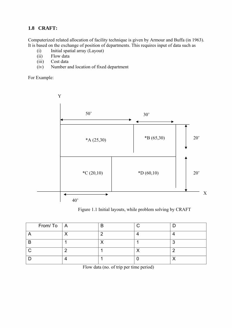
1.8 CRAFT: Computerized related allocation of facility technique is given by Armour and Buffa (in 1963). It is based on the exchange of position of departments. This requires input of data such as

(i) Initial spatial array (Layout) (ii) Flow data (iii) Cost data (iv) Number and location of fixed department

For Example:

Y

X

20’

20’

30’

*A (25,30) *B (65,30)

50’

*C (20,10)

Figure 1.1 Initial layouts, while problem solving by CRAFT

40’

*D (60,10)

From/ To A B C D

A X 2 4 4

B 1 X 1 3

C 2 1 X 2

D 4 1 0 X

Flow data (no. of trip per time period)

Assume unit cost. Cost represents the cost required to move one unit of distance between of

departments. The rectilinear distance between the current centroids for departments A and B

is

I XA –XB I + I YA –YB I = I 25 –65 I + I 30 –30 I = 40

From/ To A B C D

A X 40 25 55

B 40 X 65 25

C 25 65 X 40

D 55 25 40 X

Distance data

From/ To A B C D Total

A X 80 100 220 400

B 40 X 65 75 180

C 50 65 X 80 195

D 220 25 0 X 245

Total 310 170 165 375 1020

Total Cost Data

Table 1.1

CRAFT consider exchange of locations for those departments, which either are the same

area or have a common boarder.

(i) Only pair wise interchanges

(ii) Only three ways interchanges

(iii) Pair wise interchanges followed by three way interchanges

(iv) Three ways interchanges followed by pair wise interchanges

(v) Best of two way and three way interchanges

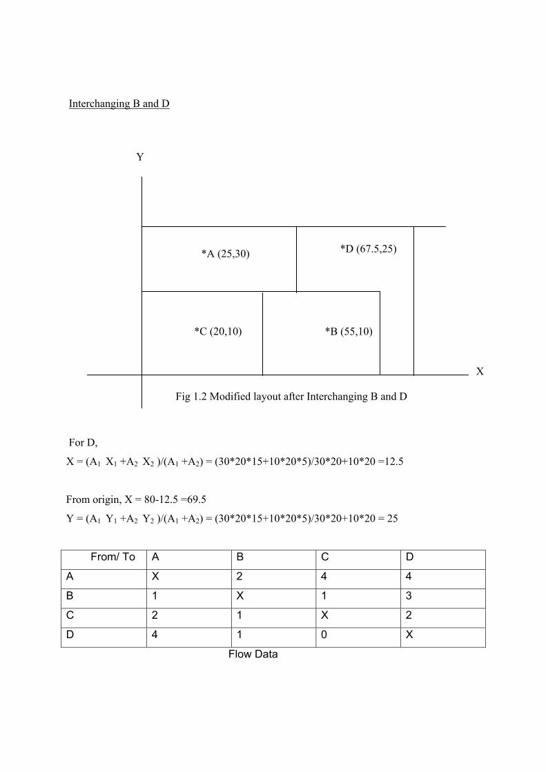
Interchanging B and D

Y

X

*A (25,30) *D (67.5,25)

Fig 1.2 Modified layout after Interchanging B and D

*B (55,10) *C (20,10)

For D,

X = (A1 X1 +A2 X2 )/(A1 +A2) = (30*20*15+10*20*5)/30*20+10*20 =12.5

From origin, X = 80-12.5 =69.5

Y = (A1 Y1 +A2 Y2 )/(A1 +A2) = (30*20*15+10*20*5)/30*20+10*20 = 25

From/ To A B C D

A X 2 4 4

B 1 X 1 3

C 2 1 X 2

D 4 1 0 X

Flow Data

From/ To A B C D

A X 50 25 47.5

B 50 X 35 27.5

C 25 35 X 62.5

D 47.5 27.5 62.5 X

Distance Data

A B C D Total

From/ To X 100 100 190 390

B 50 X 35 82.5 167.5

C 50 35 X 125 210

D 190 27.5 0 X 217.5

Total 290 162.5 135 397.5 985.0

Table 1.2 Total Cost Data

Interchanging A and B

X = (A1 X1 +A2 X2 )/(A1 +A2) = (30*20*15+10*20*5)/30*20+10*20 =12.5

Y

X

Fig 1.3 Modified layouts after Interchanging A and B

*A (60,10) *C (20,10)

*D (65,30)

*B (15,30)

From origin, X = 70-21.5=49

Y = (A1 Y1 +A2 Y2 )/(A1 +A2) =18

From/ To A B C D

A X 2 4 4

B 1 X 1 3

C 2 1 X 2

D 4 1 0 X

Flow Data

From/ To A B C D

A X 46 37 25.5

B 46 X 25 57.5

C 37 25 X 62.5

D 25.5 57.5 62.5 X

Distance Data

A B C D Total

From/ To X 92 148 102 342

B 46 X 25 172.5 243.5

C 74 25 X 125 224

D 102 57.5 0 X 159.5

Total 222 174.5 173 375 969.0

Table 1.3 Total Cost

Interchanging C and D

Y

X

Fig 1.5 Modified layout after Interchanging C and D

*A (49,18) *D (20,10)

*C (67.5,25) *B

(15,30)

From/ To A B C D

A X 2 4 4

B 1 X 1 3

C 2 1 X 2

D 4 1 0 X

Flow Data

From/ To A B C D

A X 46 25.5 37

B 46 X 57.5 25

C 25.5 57.5 X 62.5

D 37 25 62.5 X

Distance Data

A B C D Total

From/ To X 92 102 148 342

B 46 X 57.5 75 178.5

C 51 57.5 X 125 233.5

D 148 25 0 X 173

Total 245 174.5 159.5 348 927

Table 1.4 Total Cost

1.9 Corelap: Computerized relationship layout planning, given by Lee And Moore

(1967)

Relationship Rating Meaning Meaning

A Absolutely Necessary 6

E Essential 5

I Important 4

O Ordinary important 3

U Unimportant 2

X Unimportant 1

Table 1.6 Corelap

Activity Representation in matrix form:

Table 1.7 relative relationships rating in matrix form

A B C D E

A X A U O U

B X U O U

C X I X

D X E

E X

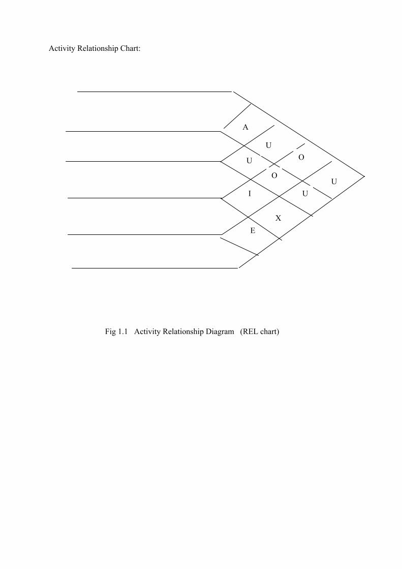
Activity Relationship Chart:

U U

O

X E

I

O

U

U

A

Fig 1.1 Activity Relationship Diagram (REL chart)

CORELAP Methodology

For Department I, define TCR (total closeness rating) as

TCR i = ∑=

n

jijr

1

Where n= no. of department

rij = closeness rating between department I and j.

The department having highest TCR is selected to place in the layout. Let this

department be P.

Next the REL chart is scanned to find a department with the highest activity

relationship with the department already fixed (p). If there is tie, select the department

with highest TCR. Let this department be q. Place department q adjacent to p.

Try to locate an unsigned department with the highest activity relationship with either

p or q. Let this be department r. Department r is placed adjacent to either department p

or department q depending upon whether it has higher activity relationship with p or

q.

Repeat step 4 till all the departments are placed.

1.10 Product Layout (Line Layout)

The plant layout in which sspecial-purpose equipment are used, changeover is expensive and

lengthy, material flow approaches continuous, material handling equipment is fixed,

operators need not be as skilled is referred as product or line layout.

Production line concepts have found their greatest field of application in assembly rather than

in fabrication. This is true because the machine tools commonly have fixed machine cycles,

making it difficult to achieve balance between successive operations. The result can be poor

equipment utilization and relatively high costs when production line concepts are applied to

fabrication operation. In assembly operation where work is more likely to be manual, balance

is easier to obtain because the total job can be divided in smaller elements.

Decision to organize facilities by product:

The managerial decision to organize facilities with a product focus and a line layout involves

important requirements, and there are some consequences affecting the work force that

should be weighed carefully.

The following conditions should be met if facilities are to be organized as a product focused

system,

1. Adequate volume for reasonable equipment utilization

2. Reasonably stable product demand

3. Product standardization

4. Part interchangeability

5. Continuous supply of material

When the conditions for product- focused systems are met, significant economic advantages

can result. The production cycle is speeded up because materials approach continuous

movement. Since very little manual handling is required, the cost of material handling is low.

In-process inventories are lower compared with those of batch processing because of the

relatively fast manufacturing cycle. Because aisles are not used for material movement and

in-process storage space is minimized, less total space is commonly required than for

equivalent functional system, even though more individual pieces of equipment may be

required. Finally, the control of flow of work (production control) is greatly simplified for

product focused system because routes are direct and mechanical. No detailed scheduling of

work to individual work places and machines is required because each operation is an integral

part of line. Scheduling the line as a whole automatically schedules the component operation.

1.11 Cellular Manufacturing

Cellular Manufacturing is a model for workplace design and is an integral part of lean

manufacturing systems. The goal of lean manufacturing is the aggressive minimization of

waste (or, more precisely, muda) in order to achieve maximum efficiency of resources.

Cellular manufacturing, sometimes called cellular or cell production, arranges factory floor

labor into semi-autonomous and multi-skilled teams, or work cells, which would manufacture

entire (simple) products or discreet (complex) product components. The semi-autonomous

and self-managed cells, if properly trained and implemented, are more flexible and

responsive than the traditional mass production line, and therefore in a better position to

manage processes, defects, scheduling, equipment maintenance, etc.

History Cellular manufacturing is a fairly new application of group technology. Group technology is

a management strategy with long-term goals of staying in business, growing, and making

profits. Companies are under relentless pressure to reduce costs while meeting the high

quality expectations of the customer to maintain a competitive advantage. Cellular

manufacturing, where properly implemented, is able to allow companies to achieve cost

savings and quality improvements, especially when combined with the other aspects of lean

manufacturing. Cell manufacturing systems are currently used to manufacture anything from

hydraulic and engine pumps used in aircraft to plastic packaging components made using

injection molding.

Design

Cellular manufacturing has the goal of having the flexibility of a high variety, low demand

production, while maintaining the high productivity of large-scale production. This is

achieved through modularity, both in process design and product design.

In terms of process, the division of the entire production process

into discreet segments, and the assignment of each segment to a work cell, introduces the

modularity of processes. If any segment of the process needs to be changed, only the

particular cell would be affected, not the entire production line. For example, if a particular

component was prone to defects, and upgrading the equipment could solve this, a new work

cell could be designed and prepared while the obsolete cell continued production. Once the

new cell is tested and ready for production, the incoming parts to and outgoing parts from the

old cell will simply be rerouted to the new cell without having to disrupt the entire production

line. In this way, work cells enable the flexibility to upgrade processes and make variations to

products to better suit customer demands without incurring (or, at least, largely reducing) the

costs of stoppages.

In terms of products, the modularity of products must match the modularity of processes.

Even though the entire production system becomes more flexible, each individual cell is still

optimized for a relatively narrow range of tasks, in order to take advantage of the mass-

production efficiencies of specialization and scale. To the extent that a large variety of

products can be designed to be assembled from a small number of modular parts, both high

product variety and high productivity can be achieved. For example, a varied range of

automobiles may be designed to use the same chassis, a small number of engine

configurations, and a moderate variety of car bodies, each available in a range of colors. In

this way, combining the outputs from a more limited number of work cells can produce a

large variety of automobiles, with different performances and appearances and functions.

In combination, each modular part is designed for a particular work cell,

or dedicated clusters of machines or manufacturing processes. Cells are usually bigger than

typical conventional workstations, but smaller than a complete conventional department.

After conversion, a cellular manufacturing layout usually requires less floor space as a result

of the optimized production processes. Each cell is responsible for its own internal control of

quality, scheduling, ordering, and record keeping. The idea is to place the responsibility of

these tasks on those who are most familiar with the situation and most able to quickly fix any

problems. The middle management no longer has to monitor the outputs and

interrelationships of every single worker, and instead only has to monitor a smaller number of

work cells and the flow of materials between them, often achieved using a system of kanban.

Implementation The biggest challenge when implementing cellular manufacturing in a company is dividing

the entire manufacturing system into cells. The issues may be conceptually divided in the

"hard" issues of equipment, material flow, layout, etc., and the "soft" issues of management,

up skilling, corporate culture, etc.

The hard issues are a matter of design and investment. The entire factory floor is

rearranged, and equipment is modified or replaced to enable cell manufacturing. The costs of

work stoppages during implementation can be considerable, and lean manufacturing literature

recommends that implementation should be phased to minimize the impacts of such

disruptions as much as possible. The rearrangement of equipment (which is sometimes bolted

to the floor or built into the factory building) or the replacement of equipment that is not

flexible or reliable enough for cell manufacturing also pose considerable costs, although it

may be justified as the upgrading obsolete equipment. In both cases, the costs have to be

justified by the cost savings that can be realistically expected from the more flexible cell

manufacturing system being introduced, and miscalculations can be disastrous.

Fig 1.2 Cellular Manufacturing Process

The soft issues are more difficult to calculate and control. The

implementation of cell manufacturing often involves employee training and the redefinition

and reassignment of jobs. Each workers in each cell should ideally be able to complete the

entire range of tasks required from that cell, and often this means being more multi-skilled

than they were previously. In addition, cells are expected to be self-managing (to some

extent), and therefore workers will have to learn the tools and strategies for effective

teamwork and management, tasks that workers in conventional factory environments are

entirely unused to. At the other end of the spectrum, the management will also find their jobs

redefined, as they must take a more "hands-off" approach to allow work cells to effectively

self-manage. Instead, the must learn to perform a more oversight and support role,

maintaining a system where work cells self-optimize through supplier-input-process-output-

customer (SIPOC) relationships. These soft issues, while difficult to pin down, pose a

considerable challenge for cell manufacturing implementation; a factory with a cell-

manufacturing layout but without cell manufacturing workers and managers is unlikely to

achieve the cell manufacturing benefits.

Benefits and Cost

There are many benefits of cellular manufacturing for a company if applied correctly. Most

immediately, processes become more balanced and productivity increases because the

manufacturing floor has been reorganized and tidied up.

Part movement, set-up time, and wait time between operations are reduced, resulting in a

reduction of work in progress inventory (which represents idle capital can be better utilized

elsewhere). Cellular manufacturing, in combination with the other lean manufacturing and

just-in-time processes, also helps eliminate overproduction by only producing items when

they are needed. The results are overall cost savings and the better control of operations.

There are some costs of implementing cellular manufacturing, however, in addition to the set-

up costs of equipment and stoppages noted above. Sometimes different work cells can require

the same machines and tools, possibly resulting in duplication causing a higher investment of

equipment and lowered machine utilization. However, this is a matter of optimization and can

be addressed through process design.

Fixed Layout: The Plant Layout In, which product remains in a fixed position, and the

personnel, material and equipment come to it and used when the product is very bulky, large,

heavy or fragile is referred as Fixed Layout.

1.12 Our Consideration:

The layout is Process layout

There are passage and inner structural wall in the layout so distance calculation

between departments is not possible by using rectilinear method. We have to use

some new method of distance calculation like nodal method or adjacency graph

method. The boundary shape of layout is rectangular, however it can be applied in any

irregular shape of area.

The only criteria of optimization have been taken as minimum material handling cost

and adjacency ratio. Here the optimization technique, which we have used, is Particle swarm optimization. The maximum no. of department is 20.However it can be used for more no. of

department.

Chapter-2 A BRIEF LITERATURE REVIEW The books and journals referred to learn about

1) Problem Representation

3) Optimization techniques 2) Inter departmental distance Calculation

2. A Brief Literature Review:

2.1 Problem Representation:

2.1.1. Four-segmented chromosome model: (Lee K-Y, Han S-N, and Roh M-I (2003)

an improved genetic algorithm for facility layout problems having inner structure walls and

passages. Computer & Operation Research 30:117–138)

Facility layout can be represented as a chromosome by an

encoding process. The chromosome can be represented as the facility layout by a decoding

process. In this study, a method to model the facility layout in a four-segmented

chromosome, including positions of passages, is proposed and is shown in Fig. 3. The 4rst

segment of the chromosome represents a sequence of facilities to be allocated. The second

segment represents areas of the facilities. The areas of the facilities are given in the same

order as the 4rst segment and are allowed to vary between their upper and lower bounds. The

third and fourth segments, respectively, represent positions of the horizontal and vertical

passages in terms of distances from the origin O in Fig. 3. The positions of the Passages are

allowed to vary between their upper and lower bounds. Fig. 3 shows an example of the

facilities layout together with the corresponding representation of the four-segmented

Chromosome.

Fig 2.1 Problem Representation

Segment 1 represents sequence of Facility.

Segment 2 represents area of Facility.

Segment 3 represents position of passage in vertical direction

Segment 4 represents position of passage in horizontal direction

2.1. 2. Fixed and Variable width column codification Model: (A. Gomez, Q.I.Fernandez,

D.De la Fuente Garcia, P.J.Garcia (2003), Using Genetic Algorithm to resolve layout

problems in facilities where there are aisles, International journal of production Economics

84(2003) 271-282)

(A) For columns with a fixed width, codification consists of assigning a number to each

department, so that each individual (layout) in the population will be made up of a string of

numbers, each of which represents a department. The position in the string shows the position

of the department in the facility; for instance (2,3,1) indicates that there are three departments

on that particular floor of the facility, and that they are in the following order: first

department 2 (one always begins in the top left-hand corner), then department 3, and finally

department 1.shows the physical representation of this individual.

The above figure shows, how departments can have unusual, irregular shapes, as a

consequence of dealing with fixed width columns. In this particular example, this can be seen

in department 3).

(B) For variable width columns all the departments will have a regular, rectangular shape,

and the possibility of a department having a ‘strange’ shape is thereby eliminated. Each

column will be of the width required for departments assigned to it to fit within the

dimensions of its surface. Codification of the individual will consist of two sub-strings. The

first sub-string will be the same as for the fixed-width columns. The second sub-string, being

of the same size of the first sub-string, will include additional information, needed to know

when to move from one column to the next. This auxiliary information will be made up of

zeros and ones. A ‘0’ will indicate that the column has not been completed, and a ‘1’ that the

department is the last one in a row, and that the column is thereby complete.

Double string is used for representing variable width column

For example:

44,, 55,, 88,, 77,, 11,, 33,, 66,, 22

0, 1, 0, 0, 0, 1, 0, 1

Table 2.1 (Double string codification)

This indicates in first column facility number 4 and 5, in second column 8,7,1,3 and in third

column facility no 6 and 2 are placed.

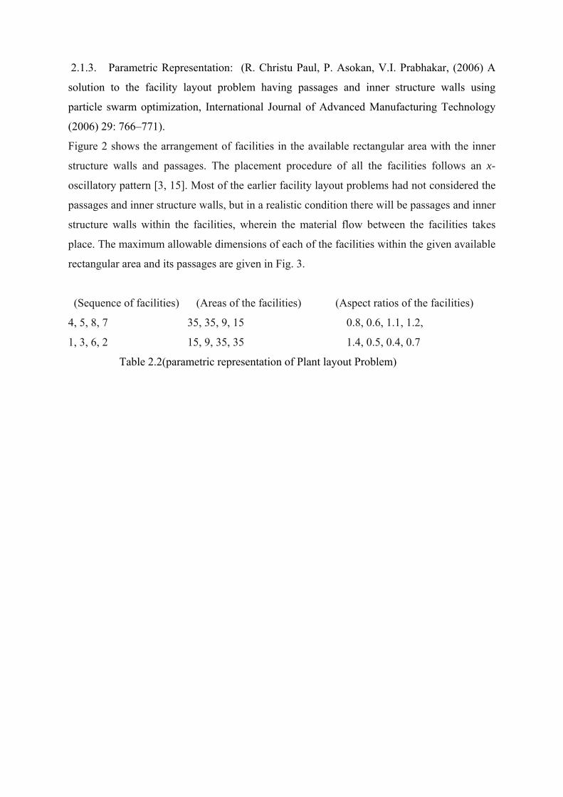
2.1.3. Parametric Representation: (R. Christu Paul, P. Asokan, V.I. Prabhakar, (2006) A

solution to the facility layout problem having passages and inner structure walls using

particle swarm optimization, International Journal of Advanced Manufacturing Technology

(2006) 29: 766–771).

Figure 2 shows the arrangement of facilities in the available rectangular area with the inner

structure walls and passages. The placement procedure of all the facilities follows an x-

oscillatory pattern [3, 15]. Most of the earlier facility layout problems had not considered the

passages and inner structure walls, but in a realistic condition there will be passages and inner

structure walls within the facilities, wherein the material flow between the facilities takes

place. The maximum allowable dimensions of each of the facilities within the given available

rectangular area and its passages are given in Fig. 3.

(Sequence of facilities) (Areas of the facilities) (Aspect ratios of the facilities)

4, 5, 8, 7 35, 35, 9, 15 0.8, 0.6, 1.1, 1.2,

1, 3, 6, 2 15, 9, 35, 35 1.4, 0.5, 0.4, 0.7

Table 2.2(parametric representation of Plant layout Problem)

2.2. Interdepartmental Distance Calculation:

2.2.1. Nodal Method of Inter Departmental distance Calculation

(R. Christu Paul, P. Asokan, V.I. Prabhakar, (2006) A solution to the facility layout problem

having passages and inner structure walls using particle swarm optimization, International

Journal of Advanced Manufacturing Technology (2006) 29: 766–771).

The rectilinear distance method cannot be employed for our problem having passages and

inner structure walls, hence a new method is employed for the distance calculation between

the facilities via the passages. In this method, some nodes are established for every facilities

as shown in Fig. 5, i.e., N1, N2, N3. . .N12. The nodes N1, N2, N3 . . . N12 are established

with respect to the length of each facility, i.e. taking the left side as the origin.

Fig 2.2 Interdepartmental Distance Calculation

A1 = 35, w1 = 3.5, l1 = 35/3.5 = 10.N1 = (l1/2) = 5. Similarly, N4 = l3 +2+(l4/2) and N6 = l3

+2+l4 +l5 + 2+(l6/2).

Hence, distance between facilities 1 and 8 will be (N10 −

N1)+4+(N11−N8)+c1+c8. Where c1 and c8 are the distance between the centroid of facility 1

and 8 from N1 and N2 respectively.

2.2.2 Adjacency Graph method Based on Dijkstra’s algorithm (Lee K-Y, Han S-N, and Roh

M-I (2003) an improved genetic algorithm for facility layout problems having inner structure

walls and passages. Computer & Operation Research 30:117–138)

Fig 2.3 Adjacency graph

The above method cannot be applied directly to a facility layout problem having passages

because materials are to be moved via the passages. The problem is the method can

miscalculate the actual distance between the facilities. For example, the distance calculated

by the rectilinear distance method between the facilities 3 and 10, (shown as a dotted line in

Fig. 4) is shorter than the actual distance (shown as a continuous line in Fig. 4). In this study

a new distance calculation method was introduced, to determine the distance between the

facilities, by using graph theory. In this new distance calculation method all relationships

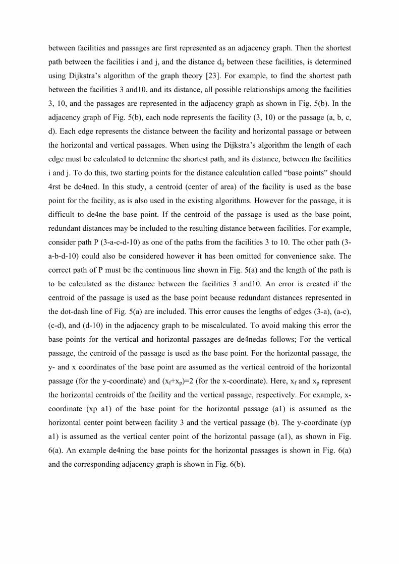
between facilities and passages are first represented as an adjacency graph. Then the shortest

path between the facilities i and j, and the distance dij between these facilities, is determined

using Dijkstra’s algorithm of the graph theory [23]. For example, to find the shortest path

between the facilities 3 and10, and its distance, all possible relationships among the facilities

3, 10, and the passages are represented in the adjacency graph as shown in Fig. 5(b). In the

adjacency graph of Fig. 5(b), each node represents the facility (3, 10) or the passage (a, b, c,

d). Each edge represents the distance between the facility and horizontal passage or between

the horizontal and vertical passages. When using the Dijkstra’s algorithm the length of each

edge must be calculated to determine the shortest path, and its distance, between the facilities

i and j. To do this, two starting points for the distance calculation called “base points” should

4rst be de4ned. In this study, a centroid (center of area) of the facility is used as the base

point for the facility, as is also used in the existing algorithms. However for the passage, it is

difficult to de4ne the base point. If the centroid of the passage is used as the base point,

redundant distances may be included to the resulting distance between facilities. For example,

consider path P (3-a-c-d-10) as one of the paths from the facilities 3 to 10. The other path (3-

a-b-d-10) could also be considered however it has been omitted for convenience sake. The

correct path of P must be the continuous line shown in Fig. 5(a) and the length of the path is

to be calculated as the distance between the facilities 3 and10. An error is created if the

centroid of the passage is used as the base point because redundant distances represented in

the dot-dash line of Fig. 5(a) are included. This error causes the lengths of edges (3-a), (a-c),

(c-d), and (d-10) in the adjacency graph to be miscalculated. To avoid making this error the

base points for the vertical and horizontal passages are de4nedas follows; For the vertical

passage, the centroid of the passage is used as the base point. For the horizontal passage, the

y- and x coordinates of the base point are assumed as the vertical centroid of the horizontal

passage (for the y-coordinate) and (xf+xp)=2 (for the x-coordinate). Here, xf and xp represent

the horizontal centroids of the facility and the vertical passage, respectively. For example, x-

coordinate (xp a1) of the base point for the horizontal passage (a1) is assumed as the

horizontal center point between facility 3 and the vertical passage (b). The y-coordinate (yp

a1) is assumed as the vertical center point of the horizontal passage (a1), as shown in Fig.

6(a). An example de4ning the base points for the horizontal passages is shown in Fig. 6(a)

and the corresponding adjacency graph is shown in Fig. 6(b).

fig 2.4 interdepartmental distance using adjacency graph

2.3 Optimization techniques used: 2.3.1 Improved Genetic Algorithm Used (Lee K-Y, Han S-N, and Roh M-I (2003) an

improved genetic algorithm for facility layout problems having inner structure walls and

passages. Computer & Operation Research 30:117–138): The algorithm proposed in this

study is based on the genetic algorithm (GA) that is currently widely used for facility layout

design, and also in other 4elds. The GA is classi4ed as an evolutionary search and

optimization technique. It is based on the premise that the design process can be regarded as

an evolutionary one. Details about the genetic algorithm can be found in many references

[21,22]. The proposed algorithm based on the GA in this study was implemented with C++

language and is shown schematically in Fig. 2.

Fig. 2.5 Scheme of the Improved Genetic algorithm for the facility layout problem having inner structure walls and passages.

2.3.2 Particle Swarm Optimization (R. Christu Paul, P. Asokan, V.I. Prabhakar, (2006) A

solution to the facility layout problem having passages and inner structure walls using

particle swarm optimization, International Journal of Advanced Manufacturing Technology

(2006) 29: 766–771):

The algorithm proposed in this study is based on the particle swarm

optimization (PSO). Particle swarm optimization (PSO) is an evolutionary computation

technique. It is based on the social behavior of animals such as bird flocking, fish schooling,

and swarm theory.

PSO is a population based optimization tool, both have fitness values

to evaluate the population, both update the population and search for the optimum with

random techniques, both systems do not guarantee success. However, unlike GA, PSO has no

evolution operators such as crossover and mutation. In PSO, particles update themselves with

internal velocity. They also have memory, which is important to the algorithm. Also, the

potential solutions, called particles, are “flown” through the problem space by following the

current optimum particles. Compared to GA, the information sharing mechanism in PSO is

significantly different. In GAs chromosomes share information with each other. So the whole

population moves like a group toward an optimal area. In PSO, only Gbest gives out the

information to others. It is a one-way information sharing mechanism. The evolution only

looks for the best solution. Compared with GA, all the particles tend to converge to the best

solution quickly even in the local version in most cases.

The advantages of PSO are that PSO is easy to implement and there

are few parameters to adjust. PSO has been successfully applied in many areas, such as

function optimization, artificial neural network training, fuzzy system control, and other areas

where GA can be applied

Start

Step 1. Initialization Step 2. Construction of solution Step 3. Local search Step 4. Velocity Updating Step 5. Termination condition

Initialize the parameter and particle

For each particle construct a complete solution

Improve each solution to a local optimum

Update velocity

Is continuation allowed?

Stop

PSO Flow Chart Fig. 2.6 Scheme of particle swarm optimization for the facility layout problem having inner structure walls and passages

Chapter-3 PARTICLE SWARM OPTIMIZATION AS AN OPTIMIZATION TOOL

Genetic Algorithm Vs PSO

PSO parameter control

PSO algorithm

3. PSO, As an Optimization Tool Particle swarm optimization (PSO) is a population based stochastic optimization

technique developed by Dr.Ebehart and Dr. Kennedy in 1995, inspired by social behavior

of bird flocking or fish schooling. PSO shares many similarities with evolutionary

computation techniques such as Genetic Algorithms (GA). The system is initialized with

a population of random solutions and searches for optima by updating generations.

However, unlike GA, PSO has no evolution operators such as crossover and mutation. In

PSO, the potential solutions, called particles, fly through the problem space by following

the current optimum particles. The detailed information will be given in following

sections. Compared to GA, the advantages of PSO are that PSO is easy to implement and

there are few parameters to adjust. PSO has been successfully applied in many areas:

function optimization, artificial neural network training, fuzzy system control, and other

areas where GA can be applied.

The remaining of the report includes six sections:

Background: artificial life.

The Algorithm

Comparisons between Genetic algorithm and PSO

Artificial neural network and PSO

PSO parameter control

1. Back Ground Artificial Life: The term "Artificial Life" (ALife) is used to describe

research into human-made systems that possess some of the essential properties of life. ALife

includes two-folded research topic.

ALife studies how computational techniques can help when studying biological phenomena

ALife studies how biological techniques can help out with computational problems

The focus of this report is on the second topic. Actually, there are already lots of

computational techniques inspired by biological systems. For example, artificial neural

network is a simplified model of human brain; genetic algorithm is inspired by the human

evolution. Here we discuss another type of biological system - social system, more

specifically, the collective behaviors of simple individuals interacting with their environment

and each other. Someone called it as swarm intelligence. All of the simulations utilized local

processes, such as those modeled by cellular automata, and might underlie the unpredictable

group dynamics of social behavior.

Some popular examples are floys and boids. Both of the simulations were created to interpret

the movement of organisms in a bird flock or fish school. These simulations are normally

used in computer animation or computer aided design. There are two popular swarm inspired

methods in computational intelligence areas: Ant colony optimization (ACO) and particle

swarm optimization (PSO). ACO was inspired by the behaviors of ants and has many

successful applications in discrete optimization problems. The particle swarm concept

originated as a simulation of simplified social system. The original intent was to graphically

simulate the choreography of bird of a bird block or fish school. However, it was found that

particle swarm model could be used as an optimizer.

3. The algorithm: As stated before, PSO simulates the behaviors of bird flocking. Suppose the

following scenario: a group of birds are randomly searching food in an area. There is only

one piece of food in the area being searched. All the birds do not know where the food is. But

they know how far the food is in each iteration. So what's the best strategy to find the food?

The effective one is to follow the bird, which is nearest to the food. PSO learned from the

scenario and used it to solve the optimization problems. In PSO, each single solution is a

"bird" in the search space. We call it "particle". All of particles have fitness values, which are

evaluated by the fitness function to be optimized, and have velocities, which direct the flying

of the particles. The particles fly through the problem space by following the current

optimum particles.

PSO is initialized with a group of random particles (solutions) and then searches for optima

by updating generations. In every iteration, each particle is updated by following two "best"

values. The first one is the best solution (fitness) it has achieved so far. (The fitness value is

also stored.) This value is called p best. Another "best" value that is tracked by the particle

swarm optimizer is the best value, obtained so far by any particle in the population. This best

value is a global best and called gbest. When a particle takes part of the population as its

topological neighbors, the best value is a local best and is called lbest. After finding the two

best values, the particle updates its velocity and positions with following equation (a) and (b).

v[] = v[] + c1 * rand() * (pbest[] - present[]) + c2 * rand() * (gbest[] - present[]) ………..(a)

present[] = present[] + v[]……………………………………… (b)

v[] is the particle velocity, present[] is the current particle (solution). pbest[] and gbest[] are

defined as stated before. rand () is a random number between (0,1). c1, c2 are learning

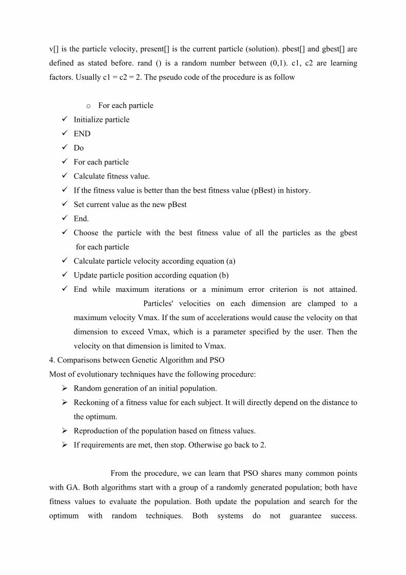
factors. Usually c1 = c2 = 2. The pseudo code of the procedure is as follow

o For each particle

Initialize particle

END

Do

For each particle

Calculate fitness value.

If the fitness value is better than the best fitness value (pBest) in history.

Set current value as the new pBest

End.

Choose the particle with the best fitness value of all the particles as the gbest

for each particle

Calculate particle velocity according equation (a)

Update particle position according equation (b)

End while maximum iterations or a minimum error criterion is not attained.

Particles' velocities on each dimension are clamped to a

maximum velocity Vmax. If the sum of accelerations would cause the velocity on that

dimension to exceed Vmax, which is a parameter specified by the user. Then the

velocity on that dimension is limited to Vmax.

4. Comparisons between Genetic Algorithm and PSO

Most of evolutionary techniques have the following procedure:

Random generation of an initial population.

Reckoning of a fitness value for each subject. It will directly depend on the distance to

the optimum.

Reproduction of the population based on fitness values.

If requirements are met, then stop. Otherwise go back to 2.

From the procedure, we can learn that PSO shares many common points

with GA. Both algorithms start with a group of a randomly generated population; both have

fitness values to evaluate the population. Both update the population and search for the

optimum with random techniques. Both systems do not guarantee success.

However, PSO does not have genetic operators like crossover and

mutation. Particles update themselves with the internal velocity. They also have memory,

which is important to the algorithm.

Compared with genetic algorithms (GAs), the information sharing mechanism in PSO is

significantly different. In GAs, chromosomes share information with each other. So the

whole population moves like a one group towards an optimal area. In PSO, only gbest (or

lbest) gives out the information to others. It is a one -way information sharing mechanism.

The evolution only looks for the best solution. Compared with GA, all the particles tend to

converge to the best solution quickly even in the local version in most cases.

5. Artificial neural network and PSO

An artificial neural network (ANN) is an analysis paradigm that is a simple model of the

brain and the back-propagation algorithm is the one of the most popular method to train the

artificial neural network. Recently there have been significant research efforts to apply

evolutionary computation (EC) techniques for the purposes of evolving one or more aspects

of artificial neural networks.

Evolutionary computation methodologies have been applied to three main

attributes of neural networks: network connection weights, network architecture (network

topology, transfer function), and network learning algorithms.

Most of the work involving the evolution of ANN has focused on the network weights and

topological structure. Usually the weights and/or topological structure are encoded as a

chromosome in GA. The selection of fitness function depends on the research goals. For a

classification problem, the rate of mis-classified patterns can be viewed as the fitness value.

The advantage of the EC is that EC can be used in cases with non-differentiable PE transfer

functions and no gradient information available.

The disadvantages are

1. The performance is not competitive in some problems.

2. Representation of the weights is difficult and the genetic operators have

to be carefully selected or developed.

There are several papers reported using PSO to replace the back-propagation learning

algorithm in ANN in the past several years. It showed PSO is a promising method to train

ANN. It is faster and gets better results in most cases. It also avoids some of the problems GA

met.

Here we show a simple example of evolving ANN with PSO. The problem is a benchmark

function of classification problem: iris data set. Measurements of four attributes of iris

flowers are provided in each data set record: sepal length, sepal width, petal length, and petal

width. Fifty sets of measurements are present for each of three varieties of iris flowers, for a

total of 150 records, or patterns.

A 3-layer ANN is used to do the classification. There are 4 inputs and 3 outputs. So the input

layer has 4 neurons and the output layer has 3 neurons. One can evolve the number of hidden

neurons. However, for demonstration only, here we suppose the hidden layer has 6 neurons.

We can evolve other parameters in the feed-forward network. Here we only evolve the

network weights. So the particle will be a group of weights, there are 4*6+6*3 = 42 weights,

so the particle consists of 42 real numbers. The range of weights can be set to [-100, 100]

(this is just a example, in real cases, one might try different ranges). After encoding the

particles, we need to determine the fitness function. For the classification problem, we feed

all the patterns to the network whose weights are determined by the particle, get the outputs

and compare it the standard outputs. Then we record the number of misclassified patterns as

the fitness value of that particle. Now we can apply PSO to train the ANN to get lower

number of misclassified patterns as possible. There are not many parameters in PSO need to

be adjusted. We only need layers and the range of the weights to get better results in different

trials.

6. PSO parameter control

From the above case, we can learn that there are two key steps when applying PSO to

optimization problems:

The representation of the solution

The fitness function.

One of the advantages of PSO is that PSO take real numbers as particles. It is not

like GA, which needs to change to binary encoding, or special genetic operators have to be

used. For example, we try to find the solution for f(x) = x1^2 + x2^2+x3^2, the particle can

be set as (x1, x2, x3), and fitness function is f(x). Then we can use the standard procedure to

find the optimum. The searching is a repeat process, and the stop criteria are that the

maximum iteration number is reached or the minimum error condition is satisfied.

There are not many parameter need to be tuned in PSO. Here is a list of the parameters

and their typical values.

The number of particles: the typical range is 20 - 40. Actually for most of the

problems 10 particles is large enough to get good results. For some difficult or special

problems, one can try 100 or 200 particles as well.

Dimension of particles: It is determined by the problem to be optimized,

Range of particles: It is also determined by the problem to be optimized, you can

specify different ranges for different dimension of particles.

Vmax: it determines the maximum change one particle can take during one iteration.

Usually we set the range of the particle as the Vmax for example, the particle (x1, x2,

x3) X1 belongs [-10, 10], and then Vmax = 20. Learning factors: c1 and c2 usually

equal to 2. However, other settings were also used in different papers. But usually c1

equals to c2 and ranges from [0, 4]

The stop condition: The maximum number of iterations the PSO execute and the

minimum error requirement. for example, for ANN training in previous section, we

can set the minimum error requirement is one miss-classified pattern. The maximum

number of iterations is set to 2000. This stop condition depends on the problem to be

optimized.

Global version vs. local version: we introduced two versions of PSO. Global and

local version. Global version is faster but might converge to local optimum for some

problems. Local version is a little bit slower but not easy to be trapped into local

optimum. One can use global version to get quick result and use local version to

refine the search.

Chapter-4 MODEL DELOPMENT

Input data required

Problem formulation

Optimization Algorithm used

4. Model Development: Input Data

Number of facilities to be allocated to the available area.

Available area and its boundary shape.

Area for each facility.

Number of rows.

No. of facilities in each row

Material flows (load/or quantity) between facilities.

Number and positions of inner structure walls.

Number and widths of each vertical and horizontal passage.

Position of each vertical and horizontal passage. Material flow between facilities: Data are taken from the paper (R. Christu Paul, P. Asokan, V.I. Prabhakar, (2006)) using particle swarm optimization ) Facility 1 2 3 4 5 6 7 8 1 0 15 0 0 0 5 5 10 2 15 0 25 40 100 90 80 70 3 0 25 0 0 0 20 30 200 4 0 40 0 0 30 10 0 0 5 0 100 0 30 0 50 70 20 6 5 90 20 10 50 0 5 0 7 5 80 30 0 70 5 0 10 8 10 70 200 0 200 0 10 0 Table 4.1 (Flow Matrix)

Problem Formulation

The objective is to minimize materials flow between facilities while at the same time satisfying the constraints of areas, aspect ratios of the facilities, and inner structure walls and passages. Finding the best facility layout means determining sequence and areas of the facilities to be allocated, For a particular Layout, Problem is formulated as ,

Minimize F = ∑∑ . ……………………………………..(1) = =

M

i

M

jijij df

1 1

*

g1= αi min – αi ≤ 0,…………………………………………………………...(2)

g2= αi - αi max ≤ 0, ………………………………………………………...(3)

g3= ai min – ai ≤ 0,……………………………………………………………(4)

g4= - A∑=

M

iia

1available ≤ 0,……………………………………………………..(5)

g5= αi min – αi ≤ 0,……………………………………………………………(6)

g6= αi min – αi ≤ 0,……………………………………………………………(7)

g7 = (xir - xi

i.s.w) (xii.s.w - xi

l) ≤ 0,……………………………………………...(8)

Where i, j= 1, 2, 3…….M, S= 1, 2, 3…P

fij : Material flow between the facility i and j,

dij : Distance between centroids of the facility i and j,

M: Number of the facilities,

αi : Aspect ratio of the facility i,

αi min and αi max : Lower and upper bounds of the aspect ratio αi

ai : Assigned area of the facility i,

ai min and aimax : Lower and upper bounds of the assigned area ai

Aavailable : Available area, P: Number of the inner structure walls,

Particle Swarm Optimization Algorithm

Step 1: Generate initial solution randomly for all particles by adding position

randomly.

Using formula Xij =Xmin+(Xmax-Xmin)*R (0,1), where R (0,1) is random number

between 0 and 1.

Step 2: Applying SPV (shortest position value) rule, (i.e. by sorting) we get initial

solution(Pbest).

Step3: Find best among all particles and assign this to Gbest.

Step4: Generate initial velocities randomly for all particles, similar as above

Vij =Vmin+(Vmax-Vmin)*R (0,1)

Step5: Update velocity according to

V[i] = V[i] (present) + c1 * (P best[i] – present [i]) + c2 * (Gbest [i] – present [i]).

Step6: Add velocities to the corresponding particles position, i.e.,

Present [i] (new) = Present [i] (old) + V [i].

Step7: if number of iterations < cyc Goto step5.

Step8: Ubest is the best among all Gbest If number of iterations< cond Goto step1.

Write Ubest. Stop

Chapter-5 RESULTS AND DISCUSSION

Comparison with standard data

Comparison with Research paper available

Generalized result of Programming

5. Results and Discussion

The Problem approach:

(i) Problem representation: One of the most important issue when designing the PSO

algorithm lies on its solution representation. In order to construct a direct

relationship between the problem domain and the PSO particles, we present n

number of dimensions for n number of facilities. In other words, each dimension

represents a typical job. In addition, the particle Xi t = [xi1t, xi2

t, xi3t…. xin

t]. Here

we have used SPV (shortest position value) rule to find out the best combination

of layout sequence using particle swarm optimization. Problems with 8,10,15,20

facilities have been analyzed.

S no 1 2 3 4 5 6 7 8 xi j -3.873 -3.952 0.022 -3.601 0.269 -1.394 2.444 -1.651 v i j -3.678 -3.878 0.998 -3.022 0.954 0.469 -1.194 0.229 Sequence 2 1 4 8 6 3 5 7

Table 4.2 (Problem Representation using SPV rule)

(ii) Initial Population: A population of particle is constructed randomly for PSO

algorithm

16 bits of each 8 bit size dimension is taken

Different positions are calculated by using formula

xi j = xmin + (xmax - xmin) * U(0,1)………………………………….(i) xmin = 0, xmax = 4, U(0,1) = Random number between 0 and 1.

Different velocities are calculated by using formula

vi j = vmin + (vmax - vmin) * U (0,1)………………………………………..(ii) vmin = -4, vmax = 4, U(0,1) = Random number between 0 and 1.

Generating 16 initial solutions or population by sorting on the basis of

smallest position value (SPV) rule, they the fitness value in each optimum

solution is the pbest.

S.No Sequence of facility Pbest 1 2 1 4 8 6 3 5 7 1260 2 8 5 3 4 7 6 1 2 1564.763 1 7 8 3 4 2 5 6 1435.244 5 8 6 7 4 2 3 1 1360 5 2 5 4 7 8 1 6 2 1245 6 8 5 4 2 6 1 7 3 1780 7 4 6 8 7 1 3 2 5 1675.738 5 4 7 8 1 2 3 6 1450.919 7 4 2 1 8 3 5 6 1015.4710 1 2 8 7 3 5 6 4 9946.8811 1 2 7 8 6 3 4 5 1031.8612 1 7 2 6 3 4 5 8 1189.8613 4 6 5 7 1 8 3 2 998.34 14 8 6 2 3 1 4 5 7 1150.6415 2 7 8 4 5 6 3 1 1451.2316 1 2 5 4 3 6 8 7 991.04 Table 4.3 (16 initial particle population of 8-bit size (dimension)) Thus we got the value of gbest = 991.04.

(iii) Update velocity and position in each iteration: Velocity and position are updated

by using equation

vij

t = vijt -1 + c1 * (pij

t-1 – xijt-1) + c2 * (gij

t-1 - xijt-1)

xij

t = xijt-1 + vij

t

where pij t = pbest in iteration “t’

gij t = gbest in iteration “t’

After getting new position in second iteration, we again used SPV (shortest

position value rule) .The new gbest = 981.55

After 40 iterations, we find the data is continuously diverging so terminating

from this iteration, we have the Ubest (universal best) =923.25

Following results have been achieved:

Final Testing of main program has been done for the given layout of size

(i) 8 facilities

(ii) 10 facilities

(iii) 15 facilities

(iv) 20 facilities

We got a Generalized and versatile form of the program for varying:

(i) Different area of layout.

(ii) Total number of facilitates to be allocated.

(iii) Number of rows.

(iv) Number of facilities in each row.

(v) Area of each facility.

(vi) Dimension of each passage.

After getting the result we compared with some other heuristic method like Genetic

algorithm.

List of programs

1. Generate random number

2. Generate 16 initial solutions by sorting on the basis of smallest position value (SPV)

rule.

3. Finding distance, material handling cost for each initial solution in above program.

4. Combining all program and sorting on the basis of minimum material handling cost

give the Pbest solution

5. Add velocity and then update velocity to find Gbest and Ubest.

6. Taking a number of iteration like 40, 60 or sometime 80 to get the optimum one.

7. Generalized form of program for all possible layout of given size.

Kyu-Yeul Lee’s algorithm [22] for the optimal facility layout design, which is based on the

genetic algorithm, is well known for its performance. In his study, he showed the competitive

power of his algorithm by comparing it with other existing algorithms. To evaluate the

efficiency of the proposed algorithm (particularly the PSO operations), a comparative test of

the proposed algorithm was performed with Kyu-Yeul Lee’s algorithm. For a more accurate

comparison, being made equal to those of Kyu-Yeul Lee’s algorithm modified the objective

function, the chromosome structure, and the representation method of the facility layout of

the proposed algorithm.

1. Comparison of computational result of proposed algorithm with standard Result obtained by Kyu-Yeul Lee’s genetic algorithm:

No of facilities

Formal Genetic Algorithm

Proposed PSO Algorithm

MHC Computational Time

MHC Computational Time

Computational Time ratio

8 27.225 1.9 25.125 1.5 1.27:1 10 28.012 2.5 27.225 2.1 1.19:1 15 31.175 3.2 30.102 2.9 1.11:1 20 37.198 4.0 37.002 3.7 1.39:1

Table 5.1

The results obtained are summarized in Table 5.1 where the best among 10 objective

function values, the mean of 10 objective function values, the mean of 10 computation times,

and the ratio of the computation times are shown. From Table 1 it can be seen that the

proposed algorithm is superior to Kyu-Yeul Lee’s algorithm, as there are 0.526 % better

values of best and mean objective functions produced by the proposed algorithm, and it

required 30% less computation Time.

2. Comparison of computational Result of proposed Algorithm with another algorithm (R. Christu Paul, P. Asokan, V.I. Prabhakar, (2006)) using particle swarm optimization) To evaluate the efficiency of the proposed algorithm, another comparative test of the

proposed algorithm was performed. The testing was performed for eight facilities and the

result obtained using the particle swarm optimization algorithm

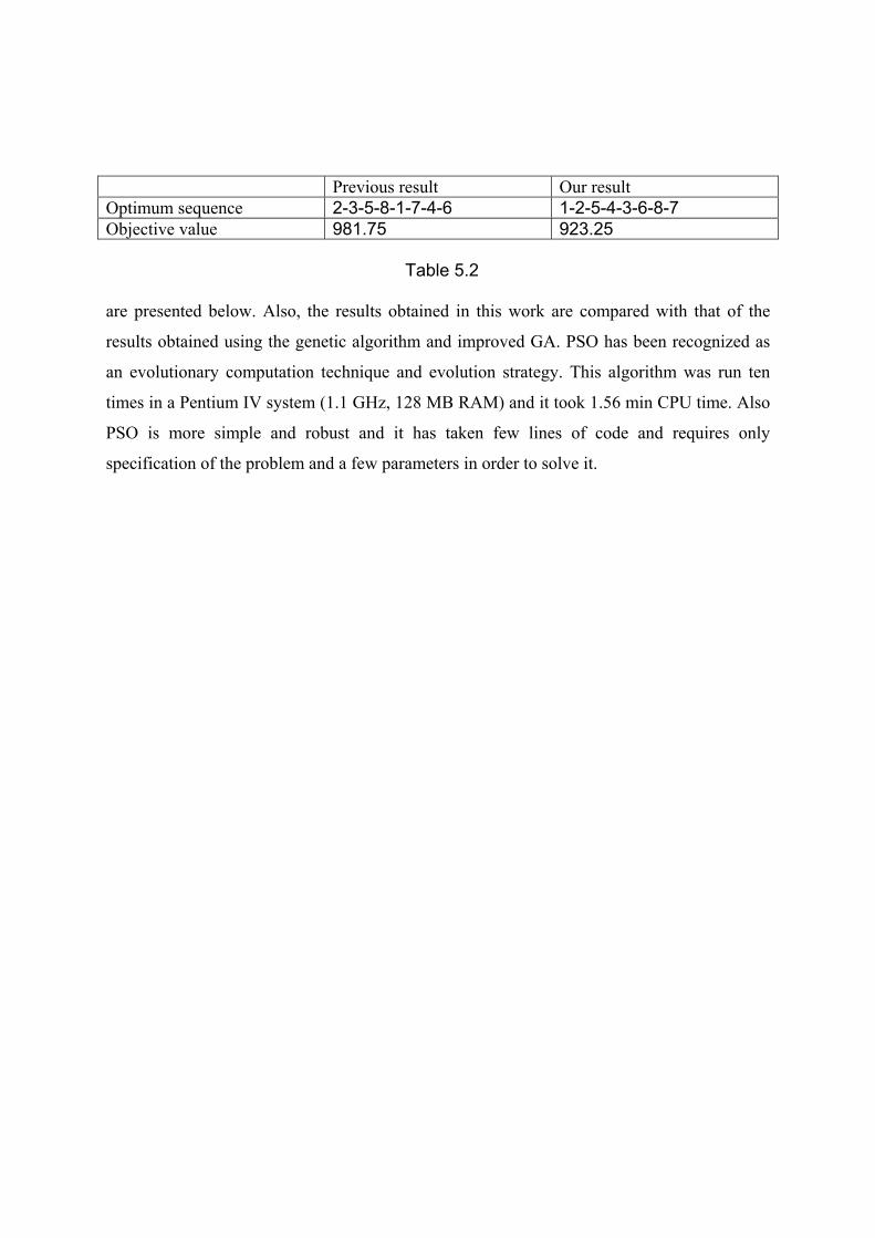
Previous result Our result Optimum sequence 2-3-5-8-1-7-4-6 1-2-5-4-3-6-8-7 Objective value 981.75 923.25 Table 5.2 are presented below. Also, the results obtained in this work are compared with that of the

results obtained using the genetic algorithm and improved GA. PSO has been recognized as

an evolutionary computation technique and evolution strategy. This algorithm was run ten

times in a Pentium IV system (1.1 GHz, 128 MB RAM) and it took 1.56 min CPU time. Also

PSO is more simple and robust and it has taken few lines of code and requires only

specification of the problem and a few parameters in order to solve it.

Chapter-6 Finding, Recommendation and future scope

Can be used in every layout planning problem

Generalized and versatile form

Some other programming language can be

more efficient

6. Finding, Recommendation and future scope

In this study, the efficient facility layout algorithm was proposed for

solving the facility layout problem having inner structure walls and passages. The facility

layout problem with inner structure walls and passages was mathematically formulated. The

layout of facilities was modeled in a four-segmented chromosome, this included positions of

passages. A method was proposed for calculating distances between the facilities using the

Nodal method. A comparison with an existing algorithm was performed to evaluate the

proposed algorithm’s efficiency. The comparison results show that the proposed algorithm is

superior to the existing one.

Interestingly a generalized approach of plant layout problem is

proposed which seems to be unique as far as my knowledge is concerned. So this result may

be used for any plant layout problem. The approach is the best for the rectangular or any

simple shape of layout but for complex shape, it becomes more complicated, specially inter

departmental distance calculation is difficult.

Since the relative advantage of a department over another

depends upon situation and person to person so adjacency criteria should be carefully used.

It is recommended to use some other programming language like

java or visual BASIC for allocating facilities more than 30 or 40 in a plant location area ,

because use of C becomes very complicated in large no of facility.

References

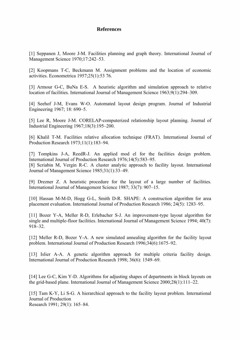
References [1] Seppanen J, Moore J-M. Facilities planning and graph theory. International Journal of Management Science 1970;17:242–53. [2] Koopmans T-C, Beckmann M. Assignment problems and the location of economic activities. Econometrica 1957;25(1):53 76. [3] Armour G-C, BuNa E-S. A heuristic algorithm and simulation approach to relative location of facilities. International Journal of Management Science 1963;9(1):294–309. [4] Seehof J-M, Evans W-O. Automated layout design program. Journal of Industrial Engineering 1967; 18: 690–5. [5] Lee R, Moore J-M. CORELAP-computerized relationship layout planning. Journal of Industrial Engineering 1967;18(3):195–200. [6] Khalil T-M. Facilities relative allocation technique (FRAT). International Journal of Production Research 1973;11(1):183–94. [7] Tompkins J-A, ReedR-J. An applied mod el for the facilities design problem. International Journal of Production Research 1976;14(5):583–95. [8] Scriabin M, Vergin R-C. A cluster analytic approach to facility layout. International Journal of Management Science 1985;31(1):33–49. [9] Drezner Z. A heuristic procedure for the layout of a large number of facilities. International Journal of Management Science 1987; 33(7): 907–15. [10] Hassan M-M-D, Hogg G-L, Smith D-R. SHAPE: A construction algorithm for area placement evaluation. International Journal of Production Research 1986; 24(5): 1283–95. [11] Bozer Y-A, Meller R-D, Erlebacher S-J. An improvement-type layout algorithm for single and multiple-floor facilities. International Journal of Management Science 1994; 40(7): 918–32. [12] Meller R-D, Bozer Y-A. A new simulated annealing algorithm for the facility layout problem. International Journal of Production Research 1996;34(6):1675–92. [13] Islier A-A. A genetic algorithm approach for multiple criteria facility design. International Journal of Production Research 1998; 36(6): 1549–69. [[14] Lee G-C, Kim Y-D. Algorithms for adjusting shapes of departments in block layouts on the grid-based plane. International Journal of Management Science 2000;28(1):111–22. [15] Tam K-Y, Li S-G. A hierarchical approach to the facility layout problem. International Journal of Production Research 1991; 29(1): 165–84.

[16] Tam K-Y. A simulated annealing algorithm for allocating space to manufacturing cells. International Journal of Production Research 1992; 30(1): 63–87. [17] Tam K-Y. Genetic algorithms, function optimization and facility layout design. European Journal of Operational Research 1992; 63(2): 322–46. [18] Tate D-M, Smith E-A. Unequal-area facility by genetic search. IIE Transactions 1995; 27(4): 465–72. [19] Goetschalckx M. An interactive layout heuristic based on hexagonal adjacency graphs. European Journal of Operational Research 1992; 63:304–21. [20] Kim J-Y, Kim Y-D. Graph theoretic heuristics for unequal-sized facility layout problems. International Journal of Management Science 1995; 23(4):391–401. [21] Goldberg D-E. Genetic algorithms in search, optimization, and machine learning. Reading, MA: Addison Wesley, 1989. [22] R. Christu Paul, P. Asokan , V.I. Prabhakar, (2006) A solution to the facility layout problem having passages and inner structure walls using particle swarm optimization , International Journal of Advanced Manufacturing Technology (2006) 29: 766–771. [23] Lee K-Y, Han S-N, Roh M-I(2003) An improved genetic algorithm for facility layout problems having inner structure walls and passages. Computer & Operation Research 30:117–138. [24] A. Gomez, Q.I.Fernandez, D.De la Fuente Garcia, P.J.Garcia (2003), Using Genetic Algorithm to resolve layout problems in facilities where there are aisles, International journal of production Economics 84(2003) 271-282. [25]. M. Fatih Tasgetiren , Mehmet Sevkli , Yun-Chia Liang and Gunes Gencyilmaz (2004), Particle Swarm Optimization Algorithm for Permutation Flow shop Sequencing Problem LNCS, Springer Berlin / Heidelberg, Volume 3172/2004, pages 382-389 [26]. G.Suresh, V.V.Vinod and S.Sahu (1995), A Genetic Algorithm for facility layout International journal of production research 33:1212, 3411-3423, Taylor & Francis, 1995. [27].Jaydeep Balakrishnan, Chuh Hang Cheng, Daniel G.Conway, Chuh Ming Lau, A hybrid Genetic Algorithm for the dynamic plant layout problem(2003), international Journal of production economics 86(2006) 107-120. [28]. Sunderesh S. Heragu (1992), Experimental Analysis of Simulated Annealing based algorithm for a layout problem, European Journal of operational research 57(1992) 190-202 [29] Marc Goetschalckx, (March 1992), An interactive layout heuristic based on hexagonal adjacency graphs, European Journal of Operational Research 63 (1992) 304-321.

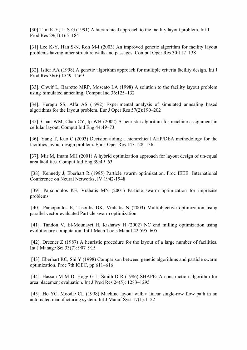
[30] Tam K-Y, Li S-G (1991) A hierarchical approach to the facility layout problem. Int J Prod Res 29(1):165–184 [31] Lee K-Y, Han S-N, Roh M-I (2003) An improved genetic algorithm for facility layout problems having inner structure walls and passages. Comput Oper Res 30:117–138 [32]. Islier AA (1998) A genetic algorithm approach for multiple criteria facility design. Int J Prod Res 36(6):1549–1569 [33]. Chwif L, Barretto MRP, Moscato LA (1998) A solution to the facility layout problem using simulated annealing. Comput Ind 36:125–132 [34]. Heragu SS, Alfa AS (1992) Experimental analysis of simulated annealing based algorithms for the layout problem. Eur J Oper Res 57(2):190–202 [35]. Chan WM, Chan CY, Ip WH (2002) A heuristic algorithm for machine assignment in cellular layout. Comput Ind Eng 44:49–73 [36]. Yang T, Kuo C (2003) Decision aiding a hierarchical AHP/DEA methodology for the facilities layout design problem. Eur J Oper Res 147:128–136 [37]. Mir M, Imam MH (2001) A hybrid optimization approach for layout design of un-equal area facilities. Comput Ind Eng 39:49–63 [38]. Kennedy J, Eberhart R (1995) Particle swarm optimization. Proc IEEE International Conference on Neural Networks, IV:1942-1948 [39]. Parsopoulos KE, Vrahatis MN (2001) Particle swarm optimization for imprecise problems. [40]. Parsopoulos E, Tasoulis DK, Vrahatis N (2003) Multiobjective optimization using parallel vector evaluated Particle swarm optimization. [41]. Tandon V, El-Mounayri H, Kishawy H (2002) NC end milling optimization using evolutionary computation. Int J Mach Tools Manuf 42:595–605 [42]. Drezner Z (1987) A heuristic procedure for the layout of a large number of facilities. Int J Manage Sci 33(7): 907–915 [43]. Eberhart RC, Shi Y (1998) Comparison between genetic algorithms and particle swarm optimization. Proc 7th ICEC, pp 611–616 [44]. Hassan M-M-D, Hogg G-L, Smith D-R (1986) SHAPE: A construction algorithm for area placement evaluation. Int J Prod Res 24(5): 1283–1295 [45]. Ho YC, Moodie CL (1998) Machine layout with a linear single-row flow path in an automated manufacturing system. Int J Manuf Syst 17(1):1–22

[46] A.E. Eiben, M. Schoenauer, Evolutionary computing, Inform. Process. Lett. 82 (1)

(2002) 1–6.

[47] A.E. Eiben, J.E. Smith, Introduction to Evolutionary Computing, Springer, Berlin, 2003.

[48] J.H. Holland, Adaptation in Natural and Artificial System, The University of Michigan

Press, Ann Arbor, MI, 1975.

[49] D.E. Goldberg, Genetic Algorithms in Search, Optimization & Machine Learning,

Addison-Wesley, Reading, MA, 1989.

[50] J. Arabas, Z. Michalewicz, J. Mulawka, GAVaPS—a genetic algorithm with varying

population size, in: Proc. 1st IEEE Conf. on Evolutionary Computation, Orlando, FL, IEEE

Service Center, Piscataway, NJ, 1994, pp. 73–78.

[51] T. Bäck, A.E. Eiben, N.A.L. van der Vaart, An empirical study on GAs “without

parameters”, in: Proc. 6th Conf. on Parallel Problem Solving from Nature, Paris, France, in:

Lecture Notes in Comput. Sci., vol. 1917, Springer, Berlin, 2000, pp. 315– 324.

[52] A.E. Eiben, E. Marchiori, V.A. Valko, Evolutionary algorithms with on-the-fly

population size adjustment, in: Proc. 8th Conf. on Parallel Problem Solving from Nature,

Birmingham, UK, in: Lecture Notes in Computer Science, vol. 3242, Springer, Berlin, 2004,

pp. 41–50.

[53] J. Kennedy, R.C. Eberhart, Particle swarm optimization, in: Proc. IEEE Internat. Conf.

on Neural Networks, Perth, Australia, vol. IV, IEEE Service Center, Piscataway, NJ, 1995,

pp. 1942–1948.

[54] R.C. Eberhart, J. Kennedy, A new optimizer using particle swarm theory, in: Proc. 6th

Internat. Symp. on Micro Machine and Human Science, Nagoya, Japan, IEEE Service Center,

Piscataway, NJ, 1995, pp. 39–43.

[55] J. Kennedy, The Particle Swarm: social adaptation of knowledge, in: Proc. IEEE

Internat. Conf. on Evolutionary Computation, Indianapolis, IN, IEEE Service Center,

Piscataway, NJ, 1997, pp. 303–308.

[56] Kennedy, J., Eberhart, R.C., 1995. Particle swarm optimization. In: Proceedings of the

1995 IEEE International Conference on Neural Networks, IEEE Service Center, Piscataway,

NJ, pp. 1942–1948.

[57] Kennedy, J., Eberhart, R.C., Shi, Y. (Eds.), 2001. Swarm Intelligence.

[58] Morgan Kaufmann, San Francisco. Koziel, S., Michalewicz, Z., 1999. Evolutionary

algorithms, homomorphous mappings, and constrained parameter optimization. Evolutionary

Computation 7 (1), 19–44.

[59] Michalewicz, Z., 1995. A survey of constraint handling techniques in evolutionary

computation methods. In: McDonnell, J.R. et al. (Eds.), Proceedings of the fourth Annual

Conference on Evolutionary Programming, MIT Press, Cambridge, MA, pp. 135–155.

[60] Michalewicz, Z., Attia, N., 1994. Evolutionary optimization of constrained problems. In:

Sebald, A.V., Fogel, L.J. (Eds.), Proceedings of the third Annual Conference on Evolutionary

Programming. World Scientific, River Edge, NJ, pp. 98–108.

[61] Montes, E.M., Coello, C.A.C., 2005. A simple multi member evolution strategy to solve

constrained optimization problems. IEEE Transactions on Evolutionary computation 9 (1), 1

17.

[62] Parsopoulos, K.E., Vrahatis, M.N., 2002. Particle swarm optimization method for

constrained optimization problems. In: Kvasnicˇ ka, V. et al. (Eds), Proceedings of the second

Euro-International Symposium on Computational Intelligence, Kosˇ ice, Slovakia, pp. 214–

220.

[63] Ragsdell, K.M., Phillips, D.T., 1976. Optimal design of a class of welded structures

using geometric programming. ASME Journal of Engineering for Industries 98 (3), 1021–

1025.

[64] Rao, S.S., 1996. Engineering Optimization. Wiley, New York.