Embed Size (px)
DESCRIPTION
Design of Operations Planning and Control
Citation preview

Design of Operations Planning and ControlSystems (DOPCS)
School of Industrial EngineeringEindhoven University of Technology
Authors:J.W.M. BertrandJ.C. WortmannJ. WijngaardN.P. SuhM.M. JansenJ.C. FransooA.G. de KokT.M. de Jonge

Table of Contents
Table of Contents 1
1 Principles of Design 21.1 Introduction . . . . . . . . . . . . . . . . . . . . . . . . . . . . . . . . . . . . . . . . . . . . . 21.2 What is Design? . . . . . . . . . . . . . . . . . . . . . . . . . . . . . . . . . . . . . . . . . . . 21.3 Design Process . . . . . . . . . . . . . . . . . . . . . . . . . . . . . . . . . . . . . . . . . . . . 31.4 Functional Requirements: Definition and Characteristics . . . . . . . . . . . . . . . . . . 41.5 Constraints . . . . . . . . . . . . . . . . . . . . . . . . . . . . . . . . . . . . . . . . . . . . . . 51.6 Design Axioms . . . . . . . . . . . . . . . . . . . . . . . . . . . . . . . . . . . . . . . . . . . . 51.7 Hierarchy . . . . . . . . . . . . . . . . . . . . . . . . . . . . . . . . . . . . . . . . . . . . . . . 81.8 Designers and Their Creative Process . . . . . . . . . . . . . . . . . . . . . . . . . . . . . . 91.9 Design for Manufacture . . . . . . . . . . . . . . . . . . . . . . . . . . . . . . . . . . . . . . 10
2 Conceptual Design, Detailed Design, and Integration 122.1 Introduction . . . . . . . . . . . . . . . . . . . . . . . . . . . . . . . . . . . . . . . . . . . . . 122.2 Conceptual Design . . . . . . . . . . . . . . . . . . . . . . . . . . . . . . . . . . . . . . . . . 122.3 Detailed Design . . . . . . . . . . . . . . . . . . . . . . . . . . . . . . . . . . . . . . . . . . . 142.4 Integration and Implementation . . . . . . . . . . . . . . . . . . . . . . . . . . . . . . . . . 15
3 Hierarchical Production Planning 163.1 Introduction . . . . . . . . . . . . . . . . . . . . . . . . . . . . . . . . . . . . . . . . . . . . . 163.2 Hierarchies in Planning . . . . . . . . . . . . . . . . . . . . . . . . . . . . . . . . . . . . . . 163.3 The Eindhoven Planning Framework . . . . . . . . . . . . . . . . . . . . . . . . . . . . . . 183.4 Relation to other HPP Frameworks . . . . . . . . . . . . . . . . . . . . . . . . . . . . . . . 203.5 Uncertainty . . . . . . . . . . . . . . . . . . . . . . . . . . . . . . . . . . . . . . . . . . . . . . 213.6 Asymmetry in Supply Chain Planning, Schneeweiss’ Anticipation . . . . . . . . . . . . . 233.7 Effectuation Lead Times . . . . . . . . . . . . . . . . . . . . . . . . . . . . . . . . . . . . . . 263.8 The Need for Control . . . . . . . . . . . . . . . . . . . . . . . . . . . . . . . . . . . . . . . . 27
4 A Note on the Design of Logistics Control Systems 304.1 Introduction . . . . . . . . . . . . . . . . . . . . . . . . . . . . . . . . . . . . . . . . . . . . . 304.2 Design rules for product design. . . . . . . . . . . . . . . . . . . . . . . . . . . . . . . . . . 314.3 The Logistics Control System Design problem . . . . . . . . . . . . . . . . . . . . . . . . . 324.4 Modularity, information hiding, abstraction, and interfaces . . . . . . . . . . . . . . . . 334.5 The Production Unit Control design problem . . . . . . . . . . . . . . . . . . . . . . . . . 354.6 The Goods Flow Control Design Problem . . . . . . . . . . . . . . . . . . . . . . . . . . . . 36
Appendix A Introduction to Production Control 38
Appendix B Production Units and Goods Flow Control 55
Appendix C Goods Flow Control Structure 93
Appendix D Production Control in a Complex Component Manufacturing Firm 128
Bibliography 187
1
CHAPTER 1
Principles of Design
AcknowledgmentThis chapter is based on Chapter 1 and 2 from Principles of Design, written by N.P. Suh and usedwith his permission. Some parts are a copy from his work and other parts are modified for thepurpose of this reader.
1.1 IntroductionEven simple questions related to design cannot be answered without first understanding the natureof design, the creative processes involved in design, and the role of analysis in this process. Fur-thermore, an endless debate could follow from a discussion of design, because everyone has his orher own notion of design-related issues, just as he or she does about the common cold. Therefore,we must define several important terms such as Design, Functional Requirements (FRs), DesignParameters (DPs), and Constraints. Although it may appear cumbersome and irrelevant to considerdesign in a formal and rigid framework, the short-term burden of having to deal with the formalframework may ultimately prove beneficial.
1.2 What is Design?Design involves a continuous interplay between what we want to achieve and how we want to achieveit. For example, on a grander scale, we may say “what we want to achieve” is to go to the moon,whereas the “how” is the physical embodiment in the form of rockets and space capsules. On asmaller scale, “what we want to achieve” may be the measurement of a minute amount of moisturein plastic pellets, and “how” may be the special titration instrument. These examples show thatthe objective of design is always stated in the functional domain, whereas the physical solution (theactual operations planning and control system) is always generated in the implementation space.The design procedure involves interlinking these two domains at every hierarchical level of thedesign process. These two domains are inherently independent of each other. What relates thesetwo domains is the design.
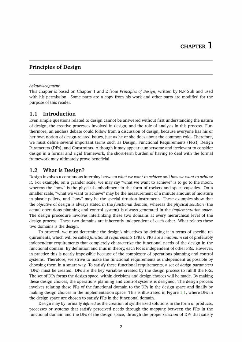
To proceed, we must determine the design’s objectives by defining it in terms of specific re-quirements, which will be called functional requirements (FRs). FRs are a minimum set of preferablyindependent requirements that completely characterize the functional needs of the design in thefunctional domain. By definition and thus in theory, each FR is independent of other FRs. However,in practice this is nearly impossible because of the complexity of operations planning and controlsystems. Therefore, we strive to make the functional requirements as independent as possible bychoosing them in a smart way. To satisfy these functional requirements, a set of design parameters(DPs) must be created. DPs are the key variables created by the design process to fulfill the FRs.The set of DPs forms the design space, within decisions and design choices will be made. By makingthese design choices, the operations planning and control systems is designed. The design processinvolves relating these FRs of the functional domain to the DPs in the design space and finally bymaking design choices in the implementation space. This is illustrated in Figure 1.1, where DPs inthe design space are chosen to satisfy FRs in the functional domain.
Design may by formally defined as the creation of synthesized solutions in the form of products,processes or systems that satisfy perceived needs through the mapping between the FRs in thefunctional domain and the DPs of the design space, through the proper selection of DPs that satisfy
2
Chapter 1. Principles of Design 3
FR1
FR2
FR3
FR 4
Functional space
Design space
DP1
DP2
DP3
DP4
DP5
DP6
Goods Flow Control
PU1 PU2 PU3
Implementation space
Figure 1.1. Design is defined as the mapping process from the functional space to the implementa-tion space to satisfy the designer-specified FRs.
FRs. This mapping process is non-unique, the actual outcome depends on a designer’s individualcreative process. Therefore, there can be an infinite number of plausible design solutions andmapping techniques. The design axioms (Section 1.6) provide the principles that the mappingtechnique must satisfy to produce a good design, and offer a basis for comparing and selectingdesigns.
1.3 Design ProcessThe design process which is illustrated in Figure 1.2, shows that the design process begins withthe recognition of a societal or business need. The need is formalized, resulting in a set of FRs inthe functional domain to satisfy the given set of needs. The selection of FRs, which defines thedesign problem, is left to the designer. Once the need is formalized, DPs are chosen, such thatall FRs are included. The structure of DPs is analyzed and compared with the original set of FRsthrough a feedback loop. When the set of DPs does not fully satisfy the specified FRs, then onemust either come up with a new set, or change the FRs to reflect the original need more accurately.This iterative process continues until the designer produces an acceptable result. The next step isto generate ideas to create an organizational structure (or a product) for the operations planningand control system. This structure is created by making design choices, i.e. by selecting a value forthe different DPs. A value can be more than a number here, it can be a decision rule for the wayproducts are taken from stock for example. In describing the design process, it was stated that thelater step is the definition of the problem to be solved in terms of FRs; that is, we must establishthe FRs from the needs that the final product or process must satisfy. This is clearly one of the mostcritical stages in the design process. This definitional step requires insight into the problem, anda knowledge base encompassing issues related to the problem. Poor problem definition leads to

Chapter 1. Principles of Design 4
unacceptable or unnecessarily complex solutions.How do we actually determine FRs to satisfy the perceived needs? There are two distinct
approaches, depending on whether we are attempting to create a major new innovation or whetherthe goal is to improve an existing design, such as a car door.
When the goal is to create design solutions that have not previously been in existence, FRsmust be defined in a solution-neutral environment; i.e., the functional space. In many cases theestablishment of an acceptable (or correct) set of FRs may require an iterative process. The mostdesirable iteration cycle, next to “no iteration”, is the reiteration at the conceptual stage of thedesign process itself, as other going through other phases with a mediocre design would be timeinefficient and, above all, extremely costly. Once the conceptual design is completed, the expectedperformance of the resultant design concept can be compared with the original perceived needs. Ifthey differ, then an improved set of FRs can be established without incurring the cost of making andtesting hardware and/or software.
One of the major problems in design is that designers do not state explicitly the FRs thattheir design must satisfy. They try to design intuitively and do not recognize the probable needto reiterate the establishment of FRs until a satisfactory design results. When a new set of FRs isestablished, the corresponding solution may be completely different from those previously tried.It may be useful to state once more the importance of proper problem definition in design: theperceived needs must be reduced to an imaginative set of FRs as the first and most critical stage ofthe design process. In the absence of a proper set of FRs, a good design is not likely to result.
The final output of the design process is information in the form of drawings, specifications,tolerances, and other relevant knowledge required to create the implementation concept. Thedesign solution should be as simple as possible, so the design output can be conveyed with minimaleffort. The total information involved should therefore be as small as possible.
1.4 Functional Requirements: Definition and CharacteristicsSince the designer can arbitrarily define the FRs to meet a certain perceived need, an acceptable setof FRs is not necessarily unique. Two designers might have chosen different sets of FRs, dependingon their judgments of the perceived needs. The implementation concept will be very differentdepending on the particular set of FRs chosen. However, in the final analysis, the implementation
Recognize &
formalize (code)
Ideate &
create
Analyze
and/or
test
Societal/
business need
Marketplace/
implementation
Compare
Reformulate
Shortcomings:
discrepancies,
failure to improve
Product attributes
Product,
prototype,
process
Functional
requirements &
constraints
Figure 1.2. The design loop. More effective synthesis requires enhanced creativity, more powerfulanalysis, and improved decision bases. (Adapted from Wilson, 1980)

Chapter 1. Principles of Design 5
concept must satisfy the perceived needs. When designing a new operations planning and controlsystem, it is difficult to choose the correct set of FRs on the first try, but we will provide the readerwith some guidelines in this reader.
Corresponding to a set of FRs, there can be many design solutions, all of which satisfy the sameset of FRs. When the original set of FRs is changed, a new solution must be found. The new solutionmay not be derived by simply modifying the previously obtained solutions that were acceptable onlyfor the original set of FRs. Many designers often make the mistake of trying to adapt or modify anexisting solution when the FRs are changed by the addition of new FRs to the original ones, ratherthan seeking a completely new solution.
To reiterate, a good designer must have the ability to choose a minimum number of FRs at eachhierarchical level of the FR tree. Some designers are proud that their design products can performmore functions than were originally specified. In this case, they have overdesigned the product.Consequently, it is more complex, more costly, and less reliable than is necessary. The designer whocreates such a solution should go back and search for a simpler solution.
1.5 ConstraintsConstraints in the context of axiomatic design represent the bounds on an acceptable solution.They are of two kinds: input constraints, which are constraints in design specifications, and systemconstraints, which are constraints imposed by the system in which the design solution must function.The input constraints are usually expressed as bounds on size, weight, materials, and cost, whereasthe system constraints are interfacial bounds such as geometric shape, capacity of machines, andeven the laws of nature.
It is sometimes difficult to determine when a certain requirement should be classified as an FRor as a constraint. In many cases cost is a constraint rather than an FR: its precise value is unimpor-tant, as long as it does not exceed a given limit. Another distinguishing feature of constraints is thatthey do not normally have tolerances associated with them, whereas FRs typically have tolerances.
As we go through the design process, zig-zagging between the functional, design and imple-mentation spaces, what used to be DPs at a higher level of the DP hierarchy may become constraintsat a lower level of the DPs hierarchy. It becomes easier to select a set of FRs when the problem ishighly constrained. The more constraints there are in a given design problem, the easier it becomesto narrow down the possible choices for FRs. In some cases the number of FRs at a given level ofthe FR hierarchy may be very small due to a large number of constraints, which should simplify thedesign process. The probability of the same set of FRs being chosen by all designers increases as thenumber of constraints is increased. As the choice for FRs decreases with the increase in constraints,the number of permutations for selecting FRs decreases, which should force convergence to a sim-ilar set of FRs. This is the case when and only when the imposed constraints on all designers areexactly identical.
1.6 Design AxiomsAs discussed in Section 1.3, the first step in design is to define a set of FRs that satisfy the perceivedneeds for an operations planning and control system. The second step is the creation of the right setof DPs. The central question is: “As we map DPs in the FR space, are there certain rules or axiomsthat are satisfied by a good design?” The uncovering of these axioms has provided significantinsight to the design process itself, and forms the scientific basis for design and synthesis (Suh et al.1978a,b).
The basic goal of the axiomatic approach is to establish a scientific foundation for the designfield, so as to provide a fundamental basis for the creation of an operations planning and con-trol system. This is a significant difference from the conventional design process, which has beendominated by empiricism and intuition. Without scientific principles, the design field will neverbe systematized, and thus will remain a subject that is difficult to comprehend, codify, teach, andpractice.

Chapter 1. Principles of Design 6
By definition, axioms are fundamental truths that are always observed to be valid and for whichthere are no counterexamples or exceptions. Axioms may be hypothesized from a large number ofobservations by noting the common phenomena shared by all cases; they cannot be proven orderived, but they can be invalidated by counterexamples or exceptions.
There are two design axioms that govern good design. Axiom 1 deals with the relationshipbetween functions and physical variables, and Axiom 2 deals with the complexity of design. Theseaxioms can be stated in a variety of semantically equivalent forms. The declarative (or procedural)form of the axioms is (Suh, 1984):
Axiom 1 The Independence AxiomMaintain the independence of FRs.
Axiom 2 The Information AxiomMinimize the information content of the design.
Axiom 1 states that during the design process, as we go from the FRs in the functional domain withDPs in the design space, the mapping must be such that a change in a particular DP must affectonly its referent FR. Axiom 2 states that, among all the designs that satisfy the Independence Axiom(Axiom 1), the one with minimum information content is the best design. The term “best” is usedin a relative sense, since there are potentially an infinite number of designs that can satisfy a givenset of FRs. Axioms 1 and 2 may be restated as follows:
Axiom 1 The Independence AxiomMaintain the independence of FRs.Alternate Statement 1: An optimal design always maintains the indepen-dence of FRs.Alternate Statement 2: In an acceptable design, the DPs and the FRs arerelated in such a way that specific DP can be adjusted to satisfy its corre-sponding FR without affecting other functional requirements.
Axiom 2 The Information AxiomMinimize the information content of the design.Alternate Statement: The best design is a functionally uncoupled designthat has the minimum information content.
Note what we stated earlier, satisfying the two Axioms stated by Suh here could only be reachedin product design or in a hypothetical and optimal situation. This is not possible for operationsplanning and control systems because these systems are very complex. Although one might striveto independent FRs, one will probably notice quickly that this is unfeasible in reality. Therefore, wewould advice to choose the FRs in a smart way by choosing a set of FRs which are as independentas possible but also such a set that the number of FRs is kept at a minimum.
The following example is provided to build understanding for the Axioms, but is not one-to-one applicable to operations planning and control systems. Take a refrigerator door design as anexample. The question is: if there are two FRs for the refrigerator door (access to the stored foodand minimal energy loss) is a vertically hung door a good design? We can see that the verticallyhung door violates Axiom 1 because the two specified FRs (i.e., access to the contents and minimumenergy use) are coupled by the proposed design. When the door is opened to take out milk, cold airin the refrigerator escapes and gives way to the warm air from outside. What, then, is an uncoupleddesign that somehow does not couple these two FRs? One such uncoupled design of the refrigeratordoor is the horizontally hinged and vertically opening door used in chest-type freezers. When thedoor is opened to take out what is inside, the cold air does not escape since cold air is heavier thanthe warm air. Therefore, this type of chest freezer door does satisfy the first axiom.
We may note here that when we refer to the satisfaction of the FRs, the solution is understoodto satisfy the original FRs within a certain tolerance band; that is, even in the case of the chest-typerefrigerator door, there is some energy loss upon removal of the contents. However, if the FR isstated so that the energy loss is to be less than 10 calories per opening of the door, and if the energyloss associated with the chest refrigerator does satisfy this requirement, then it is an acceptable
Chapter 1. Principles of Design 7
solution.
Uncoupled, coupled, and decoupledDesign can be separated into three groups: uncoupled, coupled, and decoupled (or quasi-coupled)designs. An uncoupled design satisfies Axiom 1, whereas a coupled design renders some of thefunctions dependent on other functions, and thus violates Axiom 1. A coupled design may bedecoupled; when the coupling is due to an insufficient number of DPs in comparison with thenumber of FRs that must be kept independent, we may accomplish this by adding extra components,which increases the number of DPs. A decoupled design may be inferior to an uncoupled design inthe sense that it may require additional information content.
Functional coupling should not be confused with physical coupling, which is often desirableas a consequence of Axiom 2. Integration of more than one function in a single part, as long asthe functions remain independent, should reduce complexity. An example that illustrates the useof physical integration without compromising functional independence is the bottle/can openerdesign discussed in the following example.
Suppose that we are interested in designing a simple, low cost bottle/can opener that can beoperated manually. The FRs of the device are:
FR1 = Open beverage bottles.
FR2 = Open beverage cans.
By definition, the two FRs are independent, but no mention is made of concurrency; that is, wesometimes wish to open a bottle or a can, but not both simultaneously.
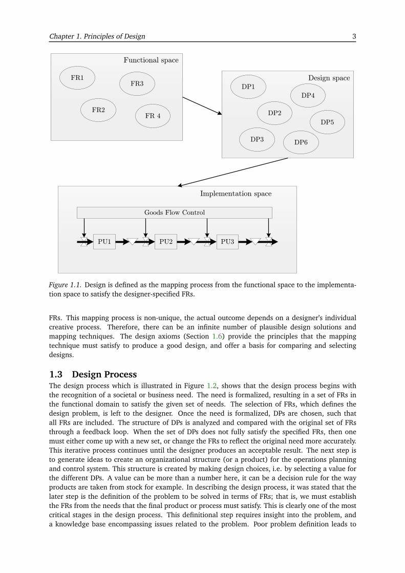
A simple device that satisfies the above set of FRs is shown in Figure 1.3. This is a very simpleopener that can be made by stamping a sheet metal strip. In this design the means for achievingthe two FRs independently are embodied in the same physical device rather than in two separatecomponents. Therefore, minimal information content is required to manufacture the device. Arethe FRs coupled by the design? The design does not couple the FRs, because the act of openingcans does not interfere with or compromise the requirement of opening bottles. The FRs wouldbe coupled only if there were an FR to open bottles and cans simultaneously, which is not thecase here. The two separate functions are fulfilled by one physical piece, but without functionalcoupling. Physical integration without functional coupling is advantageous, since the complexity ofthe product is reduced, in line with Axiom 2.
Before leaving this section, it should be noted again that the identification of the ultimate opti-mal design having minimum information content cannot be guaranteed; also, there is no method forgenerating all potential designs. We can only identify the best design on a relative basis among thoseproposed, using Axioms 1 and 2. However, the ability to eliminate unacceptable or unpromisingideas in their early stages enhances the creative part of design, and reduces the cost of developmentand the chance for failure.
Figure 1.3. Can and bottle opener. This bottle/can opener satisfies two FRs: (1) opens cans, and(2) opens bottles. If the requirement is not to perform these two functions simultaneously, then thisphysically integrated device satisfies two independent FRs.

Chapter 1. Principles of Design 8
1.7 HierarchyThere are two very important facts about design and the design process, which should be recognizedby all designers:
• FRs and DPs have hierarchies and they can be decomposed.• FRs at the i th level cannot be decomposed into the next level of the FR hierarchy without first
going over to the design space and developing a solution that satisfies the i th level FRs withall the corresponding DPs. That is, we have to travel back and forth between the functionaldomain and the design space in developing the FR and DP hierarchies.
In this section we explore these two aspects of FRs and DPs. In considering the design of a re-frigerator door in Section 1.6, we initially confined our attention to the most important problems.We considered the energy loss and the access to the food in the refrigerator. We did not concernourselves with the specific ways in which the door was to be hung, or about the insulation tech-nique. Only after we decide whether or not the door should be hung vertically should we worryabout other details. This is always the case in all design processes. The FRs and DPs can always bedecomposed into a hierarchy. Indeed, we are extremely fortunate that this is so, because we mayfocus on only a limited number of FRs at a time, thereby reducing the complexity of the design taskimmensely. The intricacy of the design task increases rapidly with the rise in the number of FRs ata given level of the FR hierarchy.
A previous discussion touched on the need to alternate between the functional domain and thedesign space in the design process. This is illustrated further here. As stated previously, the designprocess begins in the functional domain with the specification of the first level of FRs. Suppose wewish to design a passenger vehicle that can transport people within a city. We may specify the firstlevel of FRs for the vehicle to be the following:
FR1 = Ability to move forward.
FR2 = Ability to move backward.
FR3 = Ability to change directions.
FR4 = Ability to stop.
Having stated these four first-level FRs, we must now conceptualize a physical vehicle that cansatisfy them. Without completing this conceptualization process, we cannot decompose these first-level FRs further into lower level FRs. We must switch to the design space from the functionaldomain, and vice versa, in order to be able to proceed with the design process. Indeed, the designprocess requires that we switch between the functional domain and the design space each time wemove down the hierarchy. For example, in the case of the passenger vehicle, one of the solutions forsatisfying FR1 and FR2 is to use a battery-powered d.c. electrical motor and a double-pole switch.Then FR1 and FR2 can be further decomposed in the context of this implementation space.
The designer must recognize and take advantage of the existence of the functional and designhierarchies. A good designer can identify the most important FRs at each level of the functionaltree by eliminating secondary factors from consideration. Less-able designers often try to considerall the FRs of every level simultaneously, rather than making use of the hierarchical nature of FRsand DPs. Consequently, the design process becomes too complex to manage.
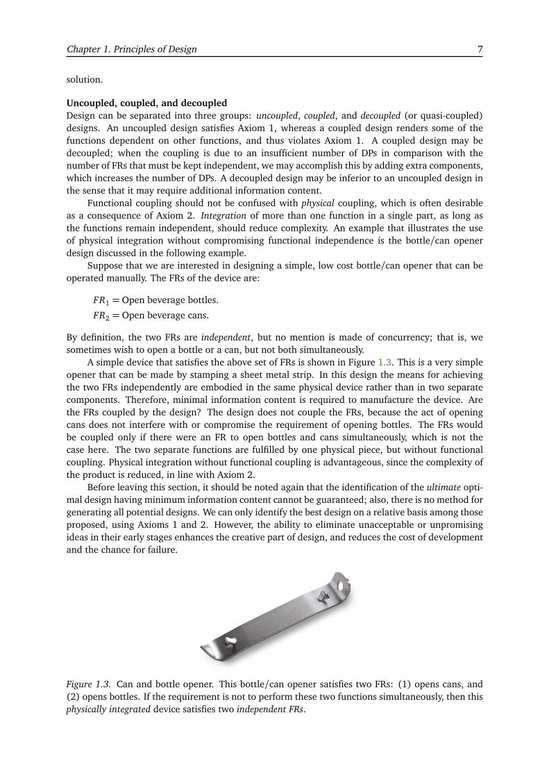
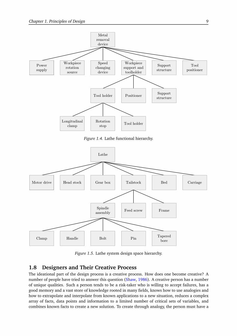
It is easier to illustrate the nature of the functional and design space hierarchy by analyzingan existing product. For example, the functional hierarchy and the design space of a lathe areshown in Figures 1.4 and 1.5 respectively. By comparing these two figures, it should be clear thatwe cannot simply construct the entire FR hierarchy without referring to the DP hierarchy at eachcorresponding level. That is, without having decided to use a tailstock, we could not have statedthe three FRs: tool holder, positioner, and support structure.
Chapter 1. Principles of Design 9
Power
supply
Metal
removal
device
Workpiece
rotation
source
Speed
changing
device
Workpiece
support and
toolholder
Support
structure
Tool
positioner
Tool holder Positioner
Power
supply
Support
structure
Tool holderRotation
stop
Longitudinal
clamp
Figure 1.4. Lathe functional hierarchy.
Power
supply
Lathe
Head stock Gear box Tailstock Bed Carriage
Spindle
assemblyFeed screw
Motor drive
Frame
PinBoltHandleTapered
boreClamp
Figure 1.5. Lathe system design space hierarchy.
1.8 Designers and Their Creative ProcessThe ideational part of the design process is a creative process. How does one become creative? Anumber of people have tried to answer this question (Shaw, 1986). A creative person has a numberof unique qualities. Such a person tends to be a risk-taker who is willing to accept failures, has agood memory and a vast store of knowledge rooted in many fields, knows how to use analogies andhow to extrapolate and interpolate from known applications to a new situation, reduces a complexarray of facts, data points and information to a limited number of critical sets of variables, andcombines known facts to create a new solution. To create through analogy, the person must have a

Chapter 1. Principles of Design 10
multidisciplinary background. Thomas Edison made many inventions using analogical techniques(Jenkins, 1987). Most inventive processes are hit-or-miss activities, requiring much trial and errorand being an alert observer. Often people chase after worthless ideas because they do not knowthat their ideas have basic flaws. The axioms described in this reader provide criteria and thusstreamline the hit-or-miss process. The axioms, particularly Axiom 1 (see Section 1.6), provideguidelines regarding the functions to be satisfied and the way in which they are to be satisfied.
There are good and not-so-good designers; one of the attributes of a good designer is theability to satisfy the perceived needs with a minimal set of independent FRs. As the number ofFRs increases, so the solution becomes more complex. Therefore, it is necessary to satisfy only theabsolutely essential functions at a given stage of design. Normally, when a problem is presented toa designer, it looks very complicated, with, a large number of variables. A good designer has theability to identify only the most important requirements and ignore those of secondary importancefor consideration at a later stage. This ability requires a broad as well as an in-depth grasp of theissues involved. This ability can be cultivated, but only with great difficulty.
Furthermore, a good designer must he able to operate in the conceptual world of the functionalas well as the implementation space. For example, the designer must know how FRs are indepen-dent of each other, in order to choose a set FRs which are least independent, avoiding unnecessarycomplexity. Many designers often evolve things that cannot be manufactured, or can be manufac-tured only with great difficulty and expense, because they do not clearly define and analyze therelationship between DPs and FRs. In order to avoid this situation, the designer must be familiarwith manufacturing processes, the laws of nature, and basic scientific principles.
The choice of FRs depends on the way in which the designer hopes to satisfy a set of needs.The determination of a good set of poorly defined perceived needs requires skill and sometimesextensive market study. This is an important step in the design process, because the final designcannot be better than the set of FRs that it was created to satisfy. In addition to the FRs, designersoften have to specify constraints. There can be many different kinds of constraints such as cost,geometrical size or weight. Often these constraints have a limiting effect on design as explainedearlier. Constraints differ from FRs in that, as long as the product designed does not exceed theconstraints, then the solution is acceptable, whereas a specific range of design values must bemaintained for each FR at all times.
1.9 Design for ManufactureIn the field of manufacturing, the most important words are productivity and reliability. Produc-tivity may be defined as the total output value of the factory divided by the total input. Althoughsuch terms as labor productivity have been used, they are becoming useless measures in modernmanufacturing operations, since the total direct labor cost is becoming a smaller fraction of thetotal manufacturing cost. Often the material is the dominant cost item, followed by indirect costsin discrete parts manufacturing. In view of the importance of productivity and reliability in manu-facturing, we need to understand the relationship between design and manufacturing.
The basic question related to design for manufacturability is: “How do we assure that the de-sign decisions incorporate manufacturing concerns?” The key answer is this: when the product andprocess designs do not harm design axioms at all levels of the FR, DP, and Process Variable (PV)hierarchies, then the product should be implementable. On the other hand, if the process or theproduct involves coupled designs, then it will be more difficult to implement, because the manu-facturing steps taken during the later stages of production can affect or undo the work of earlierstages. When the design axioms are satisfied by the product and the process, the implementabilityof the product is assured (Suh, 1985).
The design axioms can better ensure design for manufacture if we develop specific corollariesor design rules, based on the axioms, applicable to specific instances of manufacturing. Stoll (1986),in his review paper, gives the following design rules for efficient manufacture, which can be easilydeveloped for certain specific cases from the design axioms.

Chapter 1. Principles of Design 11
1. Minimize the total number of parts.2. Develop a modular design.3. Use standard components.4. Design parts to be multifunctional.5. Design parts for multi-use.6. Design parts for ease of fabrication.7. Avoid separate fasteners.8. Minimize assembly directions.9. Maximize compliance.
10. Minimize handling.
If these rules are used indiscriminately, it is obvious that the designer may act incorrectly andviolate the axioms. Therefore, if rules are to be developed, their use must be constrained to specificsituations. For example, the first rule may not be correct if the total number of parts is minimizedat the expense of coupling FRs, since this violates Axiom 1.
CHAPTER 2
Conceptual Design, Detailed Design, and Integration
2.1 IntroductionIn this chapter we explain what in designing an operations planning and control system is meantby and what has to be included in the conceptual design, the detailed design, and the integrationand implementation phase. Industrial engineering students are used to work with numbers andwould like to make calculations right from the start of a project. They will experience that thisapproach will not be helpful in designing an operation planning and control system. In designingsuch a system, (in depth) calculations are primarily made in the integration phase, in which thesecalculations are going to be automated in order to make it possible to adjust the design and quicklyrecalculate what the influence of the change in design will be. Important in designing an operationsplanning and control system is that there is a qualitative analysis which provides the right argumentsthat underpins the design made. The main task in designing a system is not to make the rightcalculations, but to design a system which is robust for changes in the environment and at the sametime provides the best performance.
The explanation in this chapter is focused on a production system. However, this will notsay that the structure cannot be used in designing other kind of systems. We have already seensuccessful applications of this design structure in the spare parts and transport industry. The finaldesign one makes, has to state exactly (in terms of rules) when to execute what process with whichresources. However, before one reaches this goal, one will experience that a huge solution spaceexists. In coping with this solution space, the rules made, the feasibility of the entire system,and the responsibilities provided to each actor in the system are extremely important to clearlydeclare. Although some design choices might not be optimal in designing an operations planningand control system, which is by definition complex, it is more important to design a system that isfeasible and satisfying the requirements, while being at the same time robust (stable and can copewith uncertainty) than an optimal system which is unstable and unreliable.
What follows in the remaining sections is an explanation of the conceptual design in Sec-tion 2.2. Next, the detailed design is explained in Section 2.3 and finally the integration andimplementation phase is explained in Section 2.4
2.2 Conceptual DesignAs mentioned before, the largest pitfall for industrial engineers who are unknown with design ofoperations planning and control systems is to start making calculations right away. The first stepone should make in designing is get an understanding of the problem. By interviewing companyemployees, experts in the field of industry or experts in designing operations planning and controlsystems, and by reading background material, one can get an throughout understanding of thecompany and of its industry.
With this knowledge, one can make the second step, which is to define the scope of the system.By setting the right boundaries, one knows what is and what is out of scope. By taking this step,all possible team members understand which processes are taken into account in the system to bedesigned. Moreover, it helps to form the right and a complete set of Functional Requirements (FRs),which is the next step.
First, one has to state the FRs for the entire system. In most cases when designing an operationsplanning and control system, this is done by setting a certain service level that has to be met, for
12
Chapter 2. Conceptual Design, Detailed Design, and Integration 13
example 95% of the orders has to be delivered within two days. Another important FR that is oftenused is to maximize the companies profits or to minimize its costs.
After stating the FRs for the entire system, one can focus on the processes that have to beexecuted in the production system. One often sees that there is a large number of processes thatis executed sequentially or in parallel. As it is too difficult to take into account the whole processat once and it is neither useful to look at each process separately, one has to define productionunits (PUs) as explained in Chapter ?? and explained in more detail in Chapter ??. By doing so,the process is decoupled, in that sense that PUs can operate (relatively) independent of each other.Independent means that for each PU FRs can be defined and that it can make its own rules regardingfor example lead times, production hours, and safety stock. The relationship between these PUs willbe determined and controlled by the Goods Flow Control (GFC), as introduced in Chapter ?? andexplained in more detail in Chapter ??. Four main reasons can be identified to decouple a processes:
• The two successive processes are not synchronized in either speed, setup or uncertainty. Whenone would not decouple these processes, it would be extremely difficult to design a feasible,controllable and thereby robust system.
• There is a difference in the opportunity to vary resources. If the resources for two processescannot or hardly be exchanged, it would not make any sense to model the two processes inthe same PU.
• There is a difference in commonality. This is, when a certain process uses a different batchsize of the products or if the product changes in a certain way that the unit used in the oneprocess is not comparable to the unit used in the other process.
• There is a difference in information available. If one or two processes have a (relatively)long lead time, new information can become available, for example a more accurate demandforecast as we show in the following example. The lead time of making cheese includingmaturation can take up to a couple of years. However, the actual demand for this cheese isnot known exactly until the customer demands the order, which can be only a few days beforetransportation to the customer (i.e. the order lead time (or customer-required lead time) ismuch shorter than the production lead time (or supply chain feasible lead time)).
After the production units have been designed, it is useful to identify the Customer Order Decou-pling Point (CODP). This point is located between two PUs and indicates the moment from whichproducts are made to order, while all (semi-finished) products till this point are made to stock andthus based on the expected demand instead of based on the actual demand. It is preferred to posi-tion this point as far as possible from the customer, as upstream (early in the complete process) aspossible. This is beneficial because actual orders are known, and production can be based on theseorders. The advantage is that products can be made for known customers and thereby (safety)stock and process times can be minimized and the service level can be maximized. However, inmost cases the production lead time will be longer than the order lead time, which forces the pointof the CODP more downstream. This is however less beneficial as one has to produce based onan estimated demand and as a consequence one may have to build (safety) stocks to meet servicelevels.
Now the production process has been divided in several PUs, modules that coordinate thedifferent PUs have to be designed. One of these units is the Goods Flow Control (GFC). This unitcoordinates the different PUs as well as for example the different stock points in the supply chain.In its function, it receives information of inventory levels and order information and provides ordersto the production units how much and when to produce to meet the FRs of the entire system. Animportant separation that has to be made in the GFC is between the detailed decisions regarding theproducts, so when to produce how much of which products and the aggregate decisions regardingthe resources, when are resources used and for which PU.
When all modules (PUs and others) have been created, FRs have to be set for each of themodules. If each of the modules meets its FRs also the entire system will meet its FRs, in a well
Chapter 2. Conceptual Design, Detailed Design, and Integration 14
designed system. These FRs can be for example that the inventory level at a certain stock point mustbe such that in 95% of (internal) demand can be satisfied from stock or that a PU must produce98% of the orders within four weeks.
In making a design, one needs to keep in mind the relation between Production and Sales asintroduced in Section ??. In many situations Production has to make what Sales has sold. However,this is not a desirable situation, which can lead to an unwanted and unstable process. Therefore,one should use the following four insights in designing an operations planning and control system,which will lead to a coordination between Production and Sales:
• Order definition. A Sales order is rarely to never the same as a Production order because ofthe positioning of the CODP as explained earlier.
• Order acceptance. It is advisable for production to make an order acceptance function. Thisis a function defined by the system designer with which Sales can determine whether an ordercan be accepted without creating an uncontrollable situation for Production.
• Seperation or responsibilities. As PUs are decoupled and operate relatively independent, somust Sales and Production work relatively independent in the sense that each department hasits own responsibilities. For example, it is not the responsibility of Sales to make a productionplan because this department has not enough insights and knowledge in Production to makethese decisions.
• Sales and Operations Planning. To make sure that there is a good coordination betweenProduction and Sales, a so called Sales and Operations Planning (S&OP) has to be organizedperiodically. In this meeting, sales orders are converted into production orders and the fore-cast of Sales is used to tune the Production planning.
Considering an order acceptance function for the system is the last step in making a conceptualdesign. Although the design now has been finished, a very important step has to be executed inmaking the conceptual design final. The feasibility in terms of lead time and capacity of the FRs setfor the modules as well as for the entire system have to be checked. In other words, it has to bechecked whether the products can be produced in the requested time and whether there is enoughcapacity to do this. One has to keep in mind that a feasible and robust system that satisfies the FRsis preferred above an optimal system. If one has defined a service level of 98%, one should notdesign a system that optimizes the service level at the expense of the robustness of the system asthis might lead to a complex and overdesigned system.
In checking the feasibility of the FRs of the modules and the entire system, key is to makesimple calculations and not to go in depth too much. In the detailed design (Section 2.3) one cando this deeper analysis. Important is that one can make a lead time analysis and that the variabilityin the demand and processes is related to the utilization (and thus capacity) by making simplecalculations (see also for formulas Hopp & Spearman (2000)). Another important point is to firstperform a feasibility check for each of the modules, after which it is easier to make a feasibilitycheck for the entire system. When the entire system is feasible and satisfactory, the conceptualdesign can be considered as final. However, this does not imply that the design cannot be changedif necessary. As one may have noticed, the number of calculations made in the conceptual design isminimal, while the qualitative analysis is crucial.
2.3 Detailed DesignThe detailed design takes the conceptual design as a staring point. In this phase the modules andstructure designed in the conceptual design is considered as given. Only in case the design can beimproved by using a certain technique, it is desirable to change the design. However, it is importantto keep in mind that a system is desired which meets the FRs.
The detailed design phase starts with understanding the conceptual model. After this, rulesare made for each of the modules such that the FRs can be met. For example, one can decideto implement the (s,S) inventory rule for a certain stock point. Another example of rules are the

Chapter 2. Conceptual Design, Detailed Design, and Integration 15
production rules First In First Out (FIFO) and Least Processing Time (LPT). Important in choosingthe right rule is that the system meets the FRs, while at the seem time staying feasible. Key isto respect the decisions made in the conceptual design. In the conceptual design PUs have beendesigned and decoupled, such that each unit can operate relatively independent. In the detaileddesign therefore rules have to be based on the information which is only locally available, i.e. thePUs cannot influence PUs and do might not know the design of other PUs. This means that a PUcan only make decisions based on the information that it receives from other sources (for exampleorders from the GFC) or information that is available in the PU itself.
During the design of rules for each of the PUs, one has to make assumptions. These assump-tions can be based on the demand of the final product or the subsequent PU) and on the supply (ofthe raw material or the previous PU). In making assumptions it is preferred that these are adaptedin an iterative way and that there is a good ground for making these assumptions.
There is a number of important factors and insights that have to considered when making thedetailed design. Important factors in designing the rules for each of the PUs are for example theset up times and set up costs (for example by using a lot sizing rule). Also the use of sequencingrules and the assessment between cost, speed, and reliability of certain resources is an importantconsideration. Lastly, also the simultaneous need of resources for certain processes can be a chal-lenging problem. For example for engineers which can be used in production as well as in testing,it is important to provide a rule to which PU they have to give priority.
As one has noticed, again in this phase a minimum to no calculations are made, it is primarilydescribing which rules have to be used in the execution of the process. So, most important is thatrules are made and that they are underpinned with arguments. These rules have to ensure that thesystem meets its FRs while at the same time the system remains feasible and stable.
2.4 Integration and ImplementationThe last phase in designing an operations planning and control system is the integration and im-plementation phase. We define integration as the coupling of the different PUs into one system andimplementation as implementing the system in a software package to test the system and to makeadjustments in case necessary. Finally, the system can be implemented in the company.
The integration of the different PUs and modules with each other is rather simple if the detaileddesign has been executed well. Whereas the total process has been decoupled, it should still be clearhow the PUs are linked to each others, which products are passed from the one PU to the other andin which form: one by one, by a batch or in a different way. Also note that a timely productionin case of, for example, an assembly process should already be incorporated in the detailed design(when to produce which product).
The implementation can still be a challenging task, also when a good detailed design is avail-able. All PUs have to be implemented in the right way and the right connections between the PUshave to be implemented. However, the first step is the decision of a proper software package basedon the goal of the implementation; a system designer might have different needs than a daily plan-ner. Regardless of the user, it is essential that the tool has a clear and user friendly dashboard onwhich the user easily can adjust the settings of the system and moreover from which it is easy toread all desired performance indicators, which can be called the input and output of the tool.
After the system has been implemented in a software tool, it should be verified and validated.Verification is checking whether the tool performs as it has to, does it provide the desired outputs.Whereas validation is the check whether the model provides an output that is reasonable with re-spect to the reality. After these checks the model can be used to calculate the performance indicatorsand (small) adjustments in conceptual of detailed design can be made to improve the designed sys-tem, i.e. increasing the system’s performance under the same or lower cost assuming the currentdesign meets the desired performance levels. When a satisfactory result has been obtained, thesystem can be implemented in the company. However, this step falls out of the design scope of thisreader.

CHAPTER 3
Hierarchical Production Planning
AcknowledgmentThis chapter contains work of the PhD Thesis of M.M. Jansen and parts of Chapter 12 from theHandbooks of Operations Research: Supply Chain Management: Design, Coordination and Operationwritten by J.C. Fransoo and A.G. de Kok. The work has been used with their permission.
3.1 IntroductionSupply Chain Planning concerns a large collection of decisions taken over time that coordinate theprimary process of a firm (or multiple firms). These decisions are taken at various organizationallevels, with various levels of detail, concerning activities over different time intervals and with dif-ferent magnitudes of (financial) implications. A classical ordering of these decisions was proposedby Anthony (1965). Anthony distinguishes three hierarchical levels of decision making: strategicplanning, tactical planning (management control), and operational control.
At the strategic level, organizational goals are established and decisions are taken about thelong term development of resources needed to achieve these goals. The decisions at this levelare aimed to guarantee the continuity of the firm and have large financial implications. Decisionsinclude for example the placement and construction of production facilities and warehouses, andthe acquisition and disposal of production equipment.
At the tactical level, it is decided how facilities and equipment are utilized to achieve the orga-nizational goals. This is the level where the Sales and Operations Planning (cf. Olhager, Rudberg,& Wikner, 2001) of the firm takes place and decisions are often directly related to the budget.Capacity levels, workforce, and aggregate production quantities for families are decided on at thislevel. Tactical decisions also include targets for stock levels and workloads, priorities, and leadtimes. If change-over of machine setups is expensive or requires considerable time, also lot-sizesare determined at this level.
At the operational level, decision making is effective on shorter time intervals and detailedinformation is available on the current and future state of the supply network and future demand.At this level, detailed plans are made and executed to meet the targets set by, and with the resourcesmade available by the tactical planning level. Decisions include the release of production orders toPUs, and the commence of activities carried out in the PUs to produce these orders to plan.
The remainder of the chapter is structured as follows. First in Section 3.2 we describe what ahierarchical production planning (HPP) is and which frameworks have been used in the past. Next,the Eindhoven Planning Framework is discussed in Section 3.3 and its relation to other frameworksin Section 3.4. In addition we describe the three different types of uncertainty common in supplynetworks in Section 3.5 of which we will explain the asymmetry of information in more detail inSection 3.6 as an introduction to the hierarchy of Schneeweiss, which can also be found in the samesection. Finally we conclude this chapter with the important concept of effectuation lead times inSection 3.7.
3.2 Hierarchies in PlanningWe define hierarchical production planning as follows: Hierarchical production planning is a struc-tural approach to the problem of coordinating activities in the primary process of the firm where the
16
Chapter 3. Hierarchical Production Planning 17
authority and responsibility to make decisions is distributed over levels and each higher level deter-mines the constraints within which lower levels are free to pursue local objectives. A hierarchicalproduction planning system adheres to the following fundamental rules:
• higher level decisions precede lower level decisions in time;• the part of the primary process of the firm that is effected by a higher level decision is not
smaller than the part that is affected by a lower level decision;• the period of time over which a higher level decision is effective is not smaller than the period
of time over which a lower level decision is effective;• the planning horizon at a higher level is not smaller than the planning horizon at a lower
level.
Decisions with regard to the different components of planning of supply chain operations have tra-ditionally been analyzed independently from one another by researchers. Research addressing thescheduling problem, the (multi-echelon) inventory problem, and the aggregate capacity planningproblem have hardly been interconnected while maintaining their own characteristics. On the con-trary, in the late 1960s and early 1970s attempts have been made from each of these domains toexpand the scope of research and apply their available specific methods to other components of thesupply chain planning problem. In these approaches, the specific nature of each of the componentshas however been disregarded, and the problems have developed into conceptually monolithicmodels. An illustration is the work on combining lot sizing and scheduling (see, e.g. Dauzère-Pérès& Lasserre, 1994), in which two models remain to exist, but a final solution is obtained by iteratingbetween the two models.
Managers were however still faced with this multitude of different problems in the supplychain planning domain. They solved these issues by organizing these decisions in a hierarchicalmanner. Meal (1984) analyzes and describes these hierarchies and links them to the hierarchicalplanning hierarchies introduced by Hax & Meal (1973) and Bitran & Hax (1977).
Decisions with regard to the planning of supply chain operations have traditionally been takenat the operational level. Meal (1984) argues that this was necessarily decentralized due to the lackof good information processing technology. In this approach, which he names the “conventionalapproach”, operations planning decisions were an integral part of the decision making power of theline managers in all parts and at all levels in the organization. Decisions were only coordinatedmarginally, and certainly not in a systematic manner. Due to the emergence of large-scale informa-tion processing technology in the 1970s, initiatives were taken to create large-scale comprehensivemodels of planning operations. Meal (1984) calls this the “centralized approach”, which is basedon a tendency to create central decision functions which are given the power to control in detail theplanning decisions of the operational process in all parts of the organization.
There are a number of difficulties associated with these centralized monolithic decision models(see also Fleischmann & Meyr (2002)). The models tend to be very big and complex. This makes theanalysis of the models and finding an optimal solution very difficult and requires a decompositionof the model in order to be able to solve this. Model decomposition is a widely used strategyin solving optimization problems. Apart from the complexity in the mathematical sense, thereare also a number of organizational and people-related difficulties associated with the centralizedapproach. The most important difficulty is that there appears to be no owner of the monolithicmodel. Responsibilities within organizations tend to be dispersed over a number of people. Themonolithic model assumes it is a single organizational unit deciding about a large number of detailsacross the entire organization. If we assume that the higher-level management would actually ownthe model and make these decisions, a number of people and model related difficulties come about:
• Detailed figures do not mean much to higher-level managers.• Detailed figures give a false sense of security because they may be highly unreliable, not only
if they refer to some future state of the system (e.g., forecast of exogenous data), but also ifthey refer to the current state of the system (data quality problems).
Chapter 3. Hierarchical Production Planning 18
• Centralized planning takes away authority from local managers further down the hierarchyand reduces their responsibility, which is not in line with the dominant management philos-ophy of self-containedness and autonomous groups. Apart from that, it is also contradictoryto a principle from control theory, which states that responsibility and decision authorityshould be matched with the opportunity to control. This last issue is extensively discussed byMcPherson & White Jr. (1994), who state that “Planning at superior levels must be consistentwith control capabilities at subordinate levels, while planning at subordinate levels must beconsistent with achieving the superior goals of the hierarchy”.
• A model never captures the complete richness of a situation. As a consequence, a local plannerdown the hierarchy will always have more information and a better representation of theactual processes than a (higher-level) model.
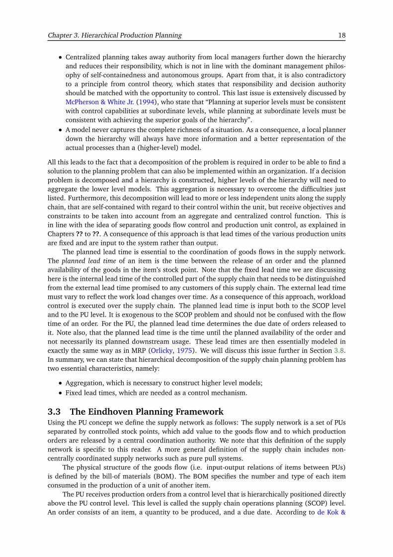
All this leads to the fact that a decomposition of the problem is required in order to be able to find asolution to the planning problem that can also be implemented within an organization. If a decisionproblem is decomposed and a hierarchy is constructed, higher levels of the hierarchy will need toaggregate the lower level models. This aggregation is necessary to overcome the difficulties justlisted. Furthermore, this decomposition will lead to more or less independent units along the supplychain, that are self-contained with regard to their control within the unit, but receive objectives andconstraints to be taken into account from an aggregate and centralized control function. This isin line with the idea of separating goods flow control and production unit control, as explained inChapters ?? to ??. A consequence of this approach is that lead times of the various production unitsare fixed and are input to the system rather than output.
The planned lead time is essential to the coordination of goods flows in the supply network.The planned lead time of an item is the time between the release of an order and the plannedavailability of the goods in the item’s stock point. Note that the fixed lead time we are discussinghere is the internal lead time of the controlled part of the supply chain that needs to be distinguishedfrom the external lead time promised to any customers of this supply chain. The external lead timemust vary to reflect the work load changes over time. As a consequence of this approach, workloadcontrol is executed over the supply chain. The planned lead time is input both to the SCOP leveland to the PU level. It is exogenous to the SCOP problem and should not be confused with the flowtime of an order. For the PU, the planned lead time determines the due date of orders released toit. Note also, that the planned lead time is the time until the planned availability of the order andnot necessarily its planned downstream usage. These lead times are then essentially modeled inexactly the same way as in MRP (Orlicky, 1975). We will discuss this issue further in Section 3.8.In summary, we can state that hierarchical decomposition of the supply chain planning problem hastwo essential characteristics, namely:
• Aggregation, which is necessary to construct higher level models;• Fixed lead times, which are needed as a control mechanism.
3.3 The Eindhoven Planning FrameworkUsing the PU concept we define the supply network as follows: The supply network is a set of PUsseparated by controlled stock points, which add value to the goods flow and to which productionorders are released by a central coordination authority. We note that this definition of the supplynetwork is specific to this reader. A more general definition of the supply chain includes non-centrally coordinated supply networks such as pure pull systems.
The physical structure of the goods flow (i.e. input-output relations of items between PUs)is defined by the bill-of materials (BOM). The BOM specifies the number and type of each itemconsumed in the production of a unit of another item.
The PU receives production orders from a control level that is hierarchically positioned directlyabove the PU control level. This level is called the supply chain operations planning (SCOP) level.An order consists of an item, a quantity to be produced, and a due date. According to de Kok &

Chapter 3. Hierarchical Production Planning 19
Parameter
setting
Supply
chain
control unit
SCOP
Aggregate Planning
Supply Chain Design
Accepted
orders
Order
acceptanceConfirmed
leadtime
Customer
orders
Supply
chain
control unit
Supply
chain
control unit
Order and resource release
Figure 3.1. Position of supply chain operations planning in the planning hierarchy.
Fransoo (2003) it is the responsibility of the SCOP level to “coordinate the release of materials andresources in the supply network under consideration such that customer service constraints are metat minimal costs.”
SCOP in most industries deals with an horizon up to several months typically with weekly timebuckets. In some industries, e.g. bulk chemicals, this function may have an horizon as short as acouple of weeks with daily buckets, whereas in other industries, e.g., pharmaceuticals, the horizonmay be as long as a couple of years with monthly time buckets. All is determined by the typicaleffectuation lead times of the industry and the lead times that customers are willing to accept.Next to the SCOP function, an order acceptance function (often called Available-To-Promise enginein current planning software) needs to be introduced in the control loop in order to control thetotal amount of work accepted by the supply chain, and to externalize the portion of the customer-perceived lead time that is due to varying demand that cannot be processed within the fixed andcontrolled lead time. Finally, a parameter setting function needs to coordinate the safety stock,lead time, and workload parameters of the supply chain. This system is depicted in Figure 3.1.Note that the functions discussed here only relate to the planning of operations, i.e. the releaseof materials and resource triggered by actual demand downstream. In this discussion, we abstainfrom other functions, such as supply chain design, the planning of seasonal or other controlledinventories, lotsizing, transportation planning, etc. For a full description of this hierarchy, we referto Fleischmann & Meyr (2002).
There is a central control of order releases in the supply network. Put differently, the bound-aries of the supply network are given by those PUs that receive their orders from a single centralcoordination authority called the SCOP function. PUs in the network need not necessarily be partof a single firm but we assume that agreements are made with subcontractors that are similar tothose made with company-owned PUs. The final stages of the supply network may operate on amake-to-order (MTO) basis. These stages are excluded from the scope of the supply network under

Chapter 3. Hierarchical Production Planning 20
consideration in this reader. All last stages in scope are thus followed by stock points that consti-tute the customer-order-decoupling-point (CODP). The items in these stock points are referred toas CODP items.
It is the task of the SCOP function to balance the supply and demand in the supply network.Specifically, it is the objective of the SCOP to satisfy demand for CODP items timely while makingefficient use of inventories and other resources in the network. In the SCOP model, marginal costsare attached to the variables corresponding to planned inventories and resource usage.
We refer to the planning framework that we have described above as the Eindhoven PlanningFramework (EPF) that is extensively described by Bertrand, Wortmann, & Wijngaard (1990) andextended by de Kok & Fransoo (2003). The framework is graphically represented in Figure 3.1.The aggregate production planning level specifies the production volume for the critical capacitiesin the PUs. Within these aggregate constraints, the SCOP level plans the order releases at itemlevel. Input to the SCOP level are furthermore the actual inventory levels in the stock points andwork-in-progress (WIP) levels in the PUs, and a detailed forecast of future CODP item demand.The SCOP function and PU control function are furthermore influenced by parameter settings thatspecify costs, service targets, safety stocks et cetera.
Two elements of the SCOP function are displayed separately in Figure 3.1. The goods flowmodel stipulates how materials are consumed and produced over time in the supply network giventhe planned lead times and the BOM. The abilities and limitations of the PU are captured in theanticipated PU model (anticipation model for short). From the perspective of SCOP, the PU is ablack box transformation of input materials into output materials. The anticipated PU model is arepresentation of the finite capacity that is used for production and is necessary for the plannedproduction to be reliable (i.e. to ensure that goods are available as planned with high probability).Anticipation is an important concept in the work of Schneeweiss (2003), whose application to theEFP we discuss in Section 3.6.
3.4 Relation to other HPP FrameworksHierarchical production planning (HPP) has various advantages over integrated or monolithic pro-duction planning. First and foremost it is in line with the prevalent industrial practice to placedecisions authority at the lowest or most decentralized part of the organization that is competent.A principle from control theory states that the authority and responsibility to make decisions shouldbe matched with the authority to control (cf. de Kok & Fransoo, 2003). Besides, detailed deci-sions made at lower organizational levels typically take effect over shorter periods of time requiringshorter planning horizons. Secondly, including all details in a single model leads to a large-scaleformulation that becomes computationally too expensive to solve. Frequent updating of the detailsexacerbates this problem. Thirdly, central collection of the data that is input to such a model is aconsiderable effort that leads to delays and high costs.
There are various frameworks described in the literature, of which the most important arethe MIT framework of hierarchical production planning (cf. Hax & Meal, 1973; Bitran, Haas, &Hax, 1981, 1982; Hax & Candea, 1984; Bitran & Tirupati, 1993) and the MRP II framework (cf.Vollmann, Berry, & Whybark, 1984). Similar frameworks are for example proposed in Miller (2002);Silver, Pyke, & Peterson (1998); Hopp & Spearman (2000). In summary, the major differences ofthe EPF with the MIT framework and the MRP II framework are the PU concept that introduceslocality in decision making (the PU needs only to consider the deployment of its own resources andnot material availability) and the concept of anticipation which allows separated decision makingfunctions.
The MIT FrameworkThe MIT framework focuses on the aggregation and disaggregation of decisions as a means of com-plexity reduction in a way that is largely analogous to decomposition techniques found in mathe-matical programming (see Shapiro, 1979, 1993). There are three levels of aggregation in the MIT

Chapter 3. Hierarchical Production Planning 21
framework: items are aggregated into families and families into types. Items of the same type aresimilar in terms of processing times and costs. Products belonging to the same family furthermoreshare the same setups on machines such that change-overs are required only when a product fromanother family needs to be produced. Finally, items may differ in characteristics such as color,packaging, and size.
Various papers treat the aggregation and disaggregation of plans (see for example Axsäter,1981, 1986; Rogers, Plante, Wong, & Evans, 1991). The main concern is to obtain plans at variouslevels that are consistent (do the quantities match) and feasible (does the detailed availability ofmaterials and resources permit a disaggregation of the plan) (cf. Gelders & van Wassenhove, 1982)).Note that these considerations are relevant only if there is no information asymmetry.
Although the MIT framework allows for management interaction at each hierarchical level,the objective of the hierarchical decomposition it to create a computationally tractable problem.Hierarchical levels are not clearly defined in terms of responsibilities and organizational scope.Decisions at various level are taken at the same moment in time and there is no difference in thetype of information available at various levels (i.e. there is no information asymmetry).
Materials Resource PlanningAnother important HPP framework is Materials Resource Planning (MRP II) which is widely used inpractice. It owes its popularity to the American Production and Inventory Control Society (APICS)who embraced MRP II as the solution to the planning of supply chain operations. Whereas theMIT framework starts from a capacity planning problem, the core of the MRP II framework ismaterials coordination. The MRP II framework has three hierarchical levels: long-range planning,intermediate-range planning and short-term planning.
The long-range planning level is an aggregate level where capacity availability is matched withthe planned production volumes. This is the level where the Sales & Operations Planning (S&OP)(cf. Olhager et al., 2001) takes place. Families of items are planned at this level that have similardemand and production requirements. The input to the S&OP process is a long term aggregateforecast of demand. The planning periods are long (e.g. a month).
At the intermediate-range level, the family planning is disaggregated into requirements for in-dividual CODP items using a detailed short-term forecast. Planning periods at this level are shorterthan at the long-range planning level (e.g. a week). The result of the disaggregation step is theMaster Production Schedule (MPS) which is subsequently translated into planned releases of or-ders through the Materials Requirements Planning algorithm. Checks for capacity and materialsavailability can take place at this level. However, these checks only create warnings (exceptions)that need to be addressed by the human planner. They are not actually taken into account in theplanning algorithm.
The short-term level is concerned with the coordination of the load of the resources. Theprimary decision taken at this level is the moment of dispatching of a job. Dispatching decisions aretaken online. That is, they are triggered by events (e.g. the completion of processing a job) and nottaken at fixed points in time. They are furthermore based on relatively simple rules (e.g. operationdue date, shortest processing time, workload rules et cetera).
In the MRP II framework, the allocation of material shortages is the responsibility of the short-term order release function. Such an allocation is clearly a myopic decision as the dispatching ofjobs does not change the MRP schedule. Consequently, materials are allocated to jobs that aredispatched first rather than to jobs that have the highest priority.
3.5 UncertaintyHopp & Spearman (2000) notice that there are two types of variation in production systems: con-trollable variation and random variation. Controllable variation is the direct consequence of deci-sions whereas random variation is beyond the control of the firm as a collective. In the setting ofHierarchical Production Planning (HPP), this definition is ambiguous. Indeed, the monolithic per-spective on production planning entails there is a single decision function. The difference between
Chapter 3. Hierarchical Production Planning 22
“controllable” and “random” is defined by whether or not the firm can influence it or not. The vari-ation concept of Hopp & Spearman is applicable to a single decision function. On the other hand,in the setting of HPP there are multiple decision functions and the question which is controllablevariation and which is random variation depends on the level in the hierarchy. More specifically, itdepends on the model used at a specific level. The distinction between controllable variation andrandom variation is thus partly a matter of the design of the HPP system.
Some events cannot be controlled directly at a specific level but can still be influenced orat least anticipated. It is therefore instructive to talk about explained variation and unexplainedvariation with regard to a specific model. Variation that is explained by a model is the part of thedynamics in the production system that is predicted by the model given the recorded state of thesystem and higher level inputs (e.g. aggregate plans, parameters, and forecasts). Variation thatis not explained is the part of the dynamics that cannot be known (a priori) or that is simply notmodeled. Note that the unexplained variation may still be controlled at a lower hierarchical level.Note furthermore that, even though the information is available, not all information is necessarilyutilized in a model whereby the part of the variation that is explained may be smaller than thepart of the variation that in principle can be explained. An example are time phased planningand scheduling models where, although it is possible to determine the occurrence of individualevents, only the aggregate number of events is accounted for in the model. Unexplained variationis often referred to as uncertainty. We distinguish three types of unexplained variation in HPP:environmental uncertainty, information asymmetry, and artefactual uncertainty which are discussedin more detail below.
It is often not possible or practical to isolate various types of uncertainty and characterize therelated variables separately. Often, the available (historic) information does not identify the precisesource of variations and even if it does, the number of observations for each specific type of variationmay be too small to characterize them reliably. Also from a modeling perspective it is preferable tolimit the different types of variation in order to keep it simple and tractable. Indeed, it is argued byHopp & Spearman (2000) that it is often not relevant to know the type of uncertainty in productionprocesses. One is typically interested in the effect of the uncertainty on the flow in the PU. It doesnot matter whether a delay in an operation is caused by unavailability of an operator or a machinebreakdown.
Environmental uncertaintyEnvironmental uncertainty is the difference between reality and the part of reality that can becaptured in a model. In most manufacturing and distribution systems literature where uncertaintyplays a role, it is considered to be an environmental phenomenon. On the one hand there is the areaof inventory management (see for example Silver et al. (1998); Zipkin (2000)) where the supplynetwork faces stochastic periodic demand and the challenge is to minimize stock levels subject tocustomer service level constraints. On the other hand there is the area of production planning (par-ticularly of job-shops, see for example Buzacott & Shanthikumar (1993); Altiok (1997)) where theproduction system faces order arrivals with stochastic times between them, where processing timesare random, and where the challenge is to balance load with capacity such that the variability ofthroughput times is controlled. Types of environmental uncertainty that are commonly consideredin manufacturing systems are:
• processing and setup time uncertainty;• capacity uncertainty;• machine break-downs;• yield uncertainty.
Processing time uncertainty is perhaps the most studied type of uncertainty, particularly in thecontext of queueing models (cf. Kleinrock, 1975; Tijms & Wiley, 2003) and queueing network mod-els (cf. Jackson, 1957; Baskett, Chandy, Muntz, & Palacios, 1975; Whitt, 1983; Bitran & Tirupati,
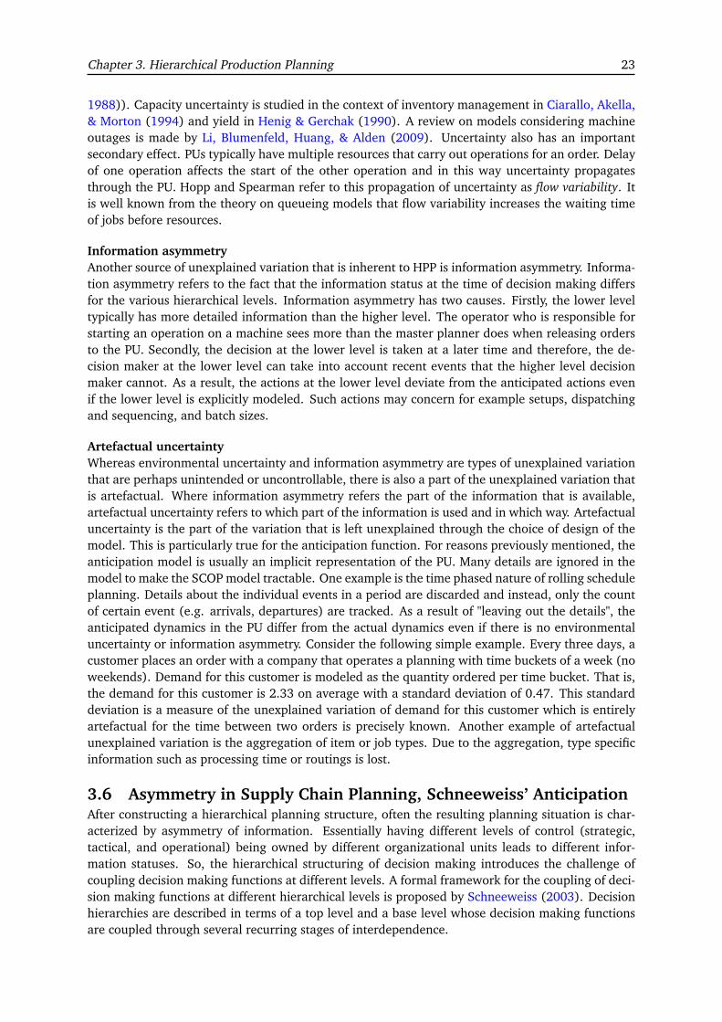
Chapter 3. Hierarchical Production Planning 23
1988)). Capacity uncertainty is studied in the context of inventory management in Ciarallo, Akella,& Morton (1994) and yield in Henig & Gerchak (1990). A review on models considering machineoutages is made by Li, Blumenfeld, Huang, & Alden (2009). Uncertainty also has an importantsecondary effect. PUs typically have multiple resources that carry out operations for an order. Delayof one operation affects the start of the other operation and in this way uncertainty propagatesthrough the PU. Hopp and Spearman refer to this propagation of uncertainty as flow variability. Itis well known from the theory on queueing models that flow variability increases the waiting timeof jobs before resources.
Information asymmetryAnother source of unexplained variation that is inherent to HPP is information asymmetry. Informa-tion asymmetry refers to the fact that the information status at the time of decision making differsfor the various hierarchical levels. Information asymmetry has two causes. Firstly, the lower leveltypically has more detailed information than the higher level. The operator who is responsible forstarting an operation on a machine sees more than the master planner does when releasing ordersto the PU. Secondly, the decision at the lower level is taken at a later time and therefore, the de-cision maker at the lower level can take into account recent events that the higher level decisionmaker cannot. As a result, the actions at the lower level deviate from the anticipated actions evenif the lower level is explicitly modeled. Such actions may concern for example setups, dispatchingand sequencing, and batch sizes.
Artefactual uncertaintyWhereas environmental uncertainty and information asymmetry are types of unexplained variationthat are perhaps unintended or uncontrollable, there is also a part of the unexplained variation thatis artefactual. Where information asymmetry refers the part of the information that is available,artefactual uncertainty refers to which part of the information is used and in which way. Artefactualuncertainty is the part of the variation that is left unexplained through the choice of design of themodel. This is particularly true for the anticipation function. For reasons previously mentioned, theanticipation model is usually an implicit representation of the PU. Many details are ignored in themodel to make the SCOP model tractable. One example is the time phased nature of rolling scheduleplanning. Details about the individual events in a period are discarded and instead, only the countof certain event (e.g. arrivals, departures) are tracked. As a result of "leaving out the details", theanticipated dynamics in the PU differ from the actual dynamics even if there is no environmentaluncertainty or information asymmetry. Consider the following simple example. Every three days, acustomer places an order with a company that operates a planning with time buckets of a week (noweekends). Demand for this customer is modeled as the quantity ordered per time bucket. That is,the demand for this customer is 2.33 on average with a standard deviation of 0.47. This standarddeviation is a measure of the unexplained variation of demand for this customer which is entirelyartefactual for the time between two orders is precisely known. Another example of artefactualunexplained variation is the aggregation of item or job types. Due to the aggregation, type specificinformation such as processing time or routings is lost.
3.6 Asymmetry in Supply Chain Planning, Schneeweiss’ AnticipationAfter constructing a hierarchical planning structure, often the resulting planning situation is char-acterized by asymmetry of information. Essentially having different levels of control (strategic,tactical, and operational) being owned by different organizational units leads to different infor-mation statuses. So, the hierarchical structuring of decision making introduces the challenge ofcoupling decision making functions at different levels. A formal framework for the coupling of deci-sion making functions at different hierarchical levels is proposed by Schneeweiss (2003). Decisionhierarchies are described in terms of a top level and a base level whose decision making functionsare coupled through several recurring stages of interdependence.
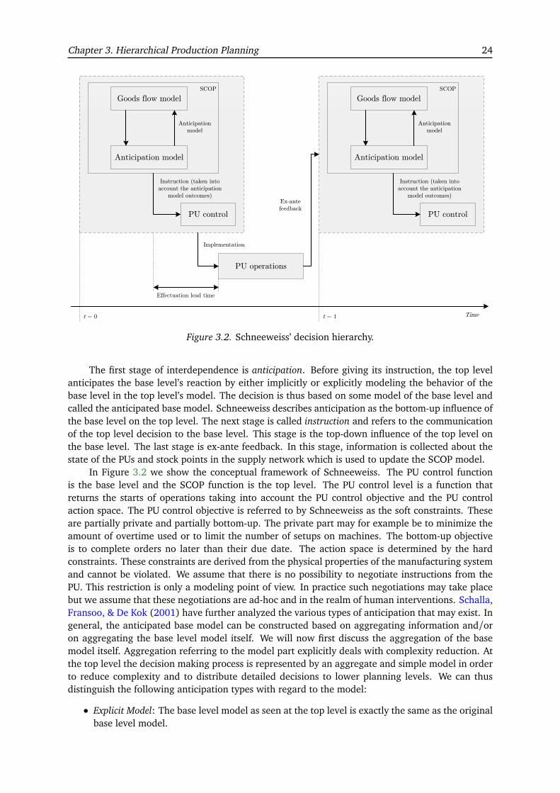
Chapter 3. Hierarchical Production Planning 24
PU operations
Instruction
Effectuation lead time
Timet = 0
Implementation
Anticipation model
Goods flow model
PU control
Anticipation
model
SCOP
Instruction (taken into
account the anticipation
model outcomes)
Anticipation model
Goods flow model
PU control
Anticipation
model
SCOP
Instruction (taken into
account the anticipation
model outcomes)
t = 1
Ex-ante
feedback
Figure 3.2. Schneeweiss’ decision hierarchy.
The first stage of interdependence is anticipation. Before giving its instruction, the top levelanticipates the base level’s reaction by either implicitly or explicitly modeling the behavior of thebase level in the top level’s model. The decision is thus based on some model of the base level andcalled the anticipated base model. Schneeweiss describes anticipation as the bottom-up influence ofthe base level on the top level. The next stage is called instruction and refers to the communicationof the top level decision to the base level. This stage is the top-down influence of the top level onthe base level. The last stage is ex-ante feedback. In this stage, information is collected about thestate of the PUs and stock points in the supply network which is used to update the SCOP model.
In Figure 3.2 we show the conceptual framework of Schneeweiss. The PU control functionis the base level and the SCOP function is the top level. The PU control level is a function thatreturns the starts of operations taking into account the PU control objective and the PU controlaction space. The PU control objective is referred to by Schneeweiss as the soft constraints. Theseare partially private and partially bottom-up. The private part may for example be to minimize theamount of overtime used or to limit the number of setups on machines. The bottom-up objectiveis to complete orders no later than their due date. The action space is determined by the hardconstraints. These constraints are derived from the physical properties of the manufacturing systemand cannot be violated. We assume that there is no possibility to negotiate instructions from thePU. This restriction is only a modeling point of view. In practice such negotiations may take placebut we assume that these negotiations are ad-hoc and in the realm of human interventions. Schalla,Fransoo, & De Kok (2001) have further analyzed the various types of anticipation that may exist. Ingeneral, the anticipated base model can be constructed based on aggregating information and/oron aggregating the base level model itself. We will now first discuss the aggregation of the basemodel itself. Aggregation referring to the model part explicitly deals with complexity reduction. Atthe top level the decision making process is represented by an aggregate and simple model in orderto reduce complexity and to distribute detailed decisions to lower planning levels. We can thusdistinguish the following anticipation types with regard to the model:
• Explicit Model: The base level model as seen at the top level is exactly the same as the originalbase level model.

Chapter 3. Hierarchical Production Planning 25
• Implicit Model: The base level model as seen at the top level is different than the original baselevel model.
Consequently, the terms explicit and implicit with regard to anticipation refer to the fact whetherthe top-level base model (including the objective functions) is exactly the same as the base-levelbase model. If this is the case, we call this explicit anticipation; if this is not the case, we call thisimplicit anticipation. Explicit anticipation thus uses a detailed model of the base level, whereasimplicit anticipation uses an aggregate model of the base level.
The second type of aggregation to construct an anticipation model is aggregation of informa-tion. This type of aggregation is related to uncertainty and effectuation time. In the context ofthe questions related to the anticipation function, special attention regarding information is paid tothe concept of information asymmetry. Information asymmetry basically entails the fact that whenmaking a decision at a higher level, the amount and quality of information may be different fromwhen the lower level decision is made (later), and again different from when the actual executionof the decision is taking place. The fact that information asymmetry exists, leads to the necessityto anticipate at a higher level decision what may happen at the lower levels decisions. We can thusdistinguish the following anticipation types with regard to information:
• Exact Information: The base level information as seen at the top level is exactly the same asthe original base level information.
• Approximate Information: The base level information as seen in the top level is different thanthe original base level information.
Consequently, the terms exact and approximate refer to the fact whether the top level model hasexact information of the base level status. Note that in most cases some time elapses between themoment at which the top level makes its decision (instruction) and the moment at which the baselevel makes its (final) decision. This difference in effectuation lead times of top level decisions andbase level decisions usually entails a difference in the information status between the top level andthe base level, resulting in information asymmetry and automatically in approximate anticipation.
Taking all combinations between anticipation types referring to the modeling part and antici-pation types referring to the information part, de Kok & Fransoo (2003) distinguish three types ofanticipation, based on the various types of aggregation used to construct the anticipation functionas discussed above. The three types are:
• Explicit Model / Exact Information (EE)• Explicit Model / Approximate Information (EA)• Implicit Model / Approximate Information (IA)
Note that the combination of exact information and implicit model does not make sense, since theredoes not seem to be a clear reason for constructing an implicit model (i.e. more aggregate than thedetailed model) if exact information is available. Further note that information asymmetry moreoften than not will lead to the fact that approximate information is the only information that can beused in the anticipatory model at the higher level. Given the fact that only approximate informationcan be used, it is not a priori clear whether the use of an explicit and detailed model is better thanthe use of an implicit model. Later, Schneeweiss (2003) distinguishes four types of anticipation:
• In explicit exact anticipation, there is no difference between the PU decision function and theanticipation model. Information asymmetry may still exist due to the fact that decisions aretaken at different points in time, but in principle the top level has access to precisely the sameinformation as the base-level.
• In explicit approximate anticipation, all aspects of the base level decision function are rep-resented in the anticipation function but some aspects are approximated. As an example,Schneeweiss mentions the replacement of a characterization of the entire distribution of arandom variable by its expectation.
Chapter 3. Hierarchical Production Planning 26
• In implicit anticipation, it is attempted to capture the "behavior" of the PU that is relevant tothe SCOP level in a model that is different from the PU decision function.
• In non-reactive anticipation, the anticipation function is effectively absent. The behavior ofthe PU is captured in generic characteristics only that do not depend on the order releasedecisions.
Non-reactive anticipation models are typically found in the inventory management literature whereit is assumed that an order has an exogenous lead time that is independent of the state of the PU andthe size of the order. A similar non-reactive anticipation model is found in Materials RequirementsPlanning (MRP).
Another example of explicit anticipation functions are iterative simulation and optimizationapproaches (see for example Hung & Leachman, 1996; Byrne & Bakir, 1999; Kim & Kim, 2001;Byrne & Hossain, 2005). If the base level follows a fixed set of rules that are precisely mappedonto the simulation model, then the simulation model can be thought of as an explicit anticipationmodel. Apart from the question to what extent it is possible and practical to develop and maintainsuch a simulation model, convergence of such iterative approaches is not guaranteed. Althoughsome favorable simulation results with respect to convergence have been found by Irdem, Kacar, &Uzsoy (2010), this convergence is not consistent in the sense that the deviations between plannedvalues and simulated values becomes smaller with each iteration.
With a few exceptions, anticipation functions for SCOP are thus implicit. Particularly, an ab-straction is made from the events occurring in continuous time. Besides, the PU control functionis typically not modeled explicitly. Resources are sometimes represented collectively by a singleaggregate resource or are omitted altogether if they are of little influence to the dynamics in thePU. Abstractions of this sort are made for several reasons. Firstly, computational tractability of theSCOP model is a concern. Secondly, detailed stipulation of the PU decision making function wouldtake away the decision authority from the PU which is in conflict with the principles of hierarchicalplanning. Besides, information asymmetry makes the detailed information upon which detaileddecisions are based uncertain. Consequently, the explicit anticipation model need not necessarilybe more accurate than the implicit anticipation model. Whereas explicit exact anticipation impliesthat it is possible to formulate a monolithic model, implicit anticipation implies the existence ofmultiple decision levels and therefore hierarchical production planning.
3.7 Effectuation Lead TimesAsymmetry in the decision making hierarchy and the necessity to anticipate is primarily caused bythe fact that it takes time to implement a decision. We will denote this time as effectuation leadtime, as introduced earlier. The effectuation lead time is the time that passes between the momenta decision is made and the moment that the consequences of this decision can be observed in theoperation of the supply chain. In supply chain planning decisions, the length of the effectuationlead times can be determined based on the product and process structure: the bill of material andthe bill of resources.
An example of an effectuation lead time is the procurement time of components. If the pro-curement lead time for a component i is Li , then ri(t), the quantity procured at the start of period tis supposed to be available for further assembly or sales at the start of period t+ Li . The immediatedecisions {ri(t)} are dependent on the exogenous demand forecasts {D̂i(t, t+ s)}, s ≥ 0, defined as:
D̂i(t, t + s) forecast of forecast of exogenous demand for item i in period t+s as decidedon at the start of period t, t ≥ 0, s ≥ 0,∀i.
Assuming supply is reliable and Li is realized, we may expect that p̂i(t, t + Li) = ri(t), where wedefine p̂ j(t, t + s) as

Chapter 3. Hierarchical Production Planning 27
p̂ j(t, t + s) forecast of quantity of item i that becomes available at the start of periodt + s as determined at the start of period t, t ≥ 0, s ≥ 0,∀i,
Reflecting the decision of the supplier to ship as late as possible. Note that p̂i(t, t + Li) is onlya planned decision from the perspective of the organization ordering the item. For the supplierthis may be either a firm decision, in case the supplier has to start immediately with processingand transporting the order for item i, or a planned decision, in case the effectuation lead timeincorporates some slack time.
Suppose that at time t the planned decision is taken according to the above equation. At thestart of period t + 1 we generate new forecasts {D̂i(t + 1, t + s)}, s ≥ 1. It is now well possible that,e.g. due to a decrease in demand for item i it is decided to change the decision made earlier, i.e.p̂i(t + 1, t + Li) 6= p̂i(t, t + Li).
Following the discussion of planned versus firm decisions, we can see that dependent on theincorporation of slack time into the procurement time, it is possible or not to change the earlierdecision. Flexibility can be further modeled by the choice of the (time-dependent) resource con-straints.
Information asymmetry itself can be described using the following example. Consider againitem i with planned lead time, i.e. the effectuation lead time of the material order release decision,Li . Often suppliers receive forecasts about future orders in some period t multiple times in orderto take consecutive decisions on e.g. buying production equipment, hiring and training people andprocurement of materials. As stated above the forecasts {D̂i(t − s, t)} for period t made at thestart of an earlier period t − s differ for different s. Thus the procurement orders derived fromthese forecasts change over time, so that the supplier’s decision to buy production equipment isbased on different information than the supplier’s decision to procure materials. This asymmetry ininformation needs to be taken into account when designing the decision hierarchy or supply chaincontrol structure. The effectuation lead time thus leads to differences between the moments in timethat certain decisions must be taken. Also, it means that decisions are often taken a substantialtime before the actual action in the physical process takes place. As a consequence the decisionmaker in fact feeds forward in terms of control theory rather than feeds back as is often suggestedin hierarchical production planning frameworks. In order to feed forward, the decision makeressentially anticipates the events over the period of time until his decision is effectuated.
It should be realized that the effectuation lead time is not only related to the bills of materialsand bills of resources, but is also a characteristic of the supply chain planning and control system.In many cases, the time buckets at higher levels of decision making are larger than at lower levels(Meal, 1984). Further, the frequency at which decisions are made, revised or processed is less athigher levels of decision making (the hierarchical structures of Gershwin (1994) are based uponthis premise). This means that changes in the actual (physical) process, e.g., changes in demand,may not be observed directly. Further, if they are observed, there may be a delay in processing theconsequences of this observation. This processing time due to the decreased frequency of decisionmaking at higher levels should be included in the effectuation lead time.
Along a time line, it clearly shows that the various SCOP decisions need to be timed alongthe lead time characteristics of the supply chain, both the physical lead time and the informationprocessing lead time. This is depicted in Figure 3.3 and was discussed in detail in Subsection 3.7.
3.8 The Need for ControlAnticipation models need to capture the base level behavior in a sufficiently accurate manner. In thissense, accurate refers to the predictive quality of the anticipation model. When designing a decisionstructure, two different approaches can be taken when constructing the anticipation functions. Thefirst approach is to try and capture the base level behavior as completely as possible by enrichingthe anticipation function by as many details as known about the base level. The second approach isto design the decision function at the base level in such a way that the actual anticipation becomes
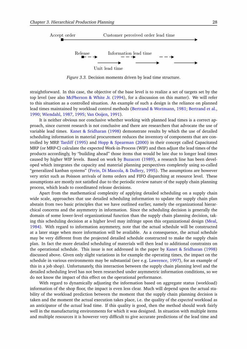
Chapter 3. Hierarchical Production Planning 28
Accept order
Release Information lead time
Unit lead time
Customer perceived order lead time
Figure 3.3. Decision moments driven by lead time structure.
straightforward. In this case, the objective of the base level is to realize a set of targets set by thetop level (see also McPherson & White Jr. (1994), for a discussion on this matter). We will referto this situation as a controlled situation. An example of such a design is the reliance on plannedlead times maintained by workload control methods (Bertrand & Wortmann, 1981; Bertrand et al.,1990; Wiendahl, 1987, 1995; Van Ooijen, 1991).
It is neither obvious nor conclusive whether working with planned lead times is a correct ap-proach, since current research is not conclusive and there are researchers that advocate the use ofvariable lead times. Kanet & Sridharan (1998) demonstrate results by which the use of detailedscheduling information in material procurement reduces the inventory of components that are con-trolled by MRP. Tardiff (1995) and Hopp & Spearman (2000) in their concept called CapacitatedMRP (or MRP-C) calculate the expected Work-in-Process (WIP) and then adjust the lead times of theproducts accordingly, by “building ahead” those items that would be late due to longer lead timescaused by higher WIP levels. Based on work by Buzacott (1989), a research line has been devel-oped which integrates the capacity and material planning perspectives completely using so-called“generalized kanban systems” (Frein, Di Mascola, & Dallery, 1995). The assumptions are howeververy strict such as Poisson arrivals of items orders and FIFO dispatching at resource level. Theseassumptions are mostly not satisfied due to the periodic review nature of the supply chain planningprocess, which leads to coordinated release decisions.
Apart from the mathematical complexity of applying detailed scheduling on a supply chainwide scale, approaches that use detailed scheduling information to update the supply chain planabstain from two basic principles that we have outlined earlier, namely the organizational hierar-chical concerns and the asymmetry in information. Since the scheduling decision is generally thedomain of some lower-level organizational function than the supply chain planning decision, tak-ing this scheduling decision at a higher level may infringe upon this organizational design (Meal,1984). With regard to information asymmetry, note that the actual schedule will be constructedat a later stage when more information will be available. As a consequence, the actual schedulemay be very different from the projected detailed schedule constructed to make the supply chainplan. In fact the more detailed scheduling of materials will then lead to additional constraints onthe operational schedule. This issue is not addressed in the paper by Kanet & Sridharan (1998)discussed above. Given only slight variations in for example the operating times, the impact on theschedule in various environments may be substantial (see e.g. Lawrence, 1997), for an example ofthis in a job shop). Unfortunately, this interaction between the supply chain planning level and thedetailed scheduling level has not been researched under asymmetric information conditions, so wedo not know the impact of this effect on the operational performance.
With regard to dynamically adjusting the information based on aggregate status (workload)information of the shop floor, the impact is even less clear. Much will depend upon the actual sta-bility of the workload prediction between the moment that the supply chain planning decision istaken and the moment the actual execution takes place, i.e. the quality of the expected workload asan anticipator of the actual lead time. If this quality is good, then the method should work fairlywell in the manufacturing environments for which it was designed. In situation with multiple itemsand multiple resources it is however very difficult to give accurate predictions of the lead time and

Chapter 3. Hierarchical Production Planning 29
to adjust the supply chain plan accordingly. This will lead to very complex models and will leadto performance and accuracy problems (Hopp & Spearman, 2000). The situation is however verydifferent when multiple actors conduct collaborative planning actions across independent compa-nies in the supply chain. In that case, the planned lead times act as a coordination aid between thevarious actors in the supply chain and planned lead times allow for independent planning of partsof the supply chain.
CHAPTER 4
A Note on the Design of Logistics Control Systems
AcknowledgmentThis Chapter is a transcription of the paper “A Note on the Design of Logistics Control Systems”written by J.W.M. Bertrand and is reproduced with his permission.
4.1 IntroductionIn this paper we present a systematic approach to the process of designing logistics control systems.Logistics has been described as "...the managerial problems raised by production, inventory anddistribution... " (preface of: Graves et al., 1993).
Since a long time logistics is a widely researched area. Among the first published results in thisfield were the determination of the economic order quantity (Harris, 1913) and the determinationof the number of servers needed in order to achieve a certain service rate (Erlang, 1917). Sincethen, and in particular after World War II, a rich flow of research has emerged in fields such asinventory control, production control, capacity control, and supply chain control, resulting in animpressive number of methods and techniques for logistics decision making for all kinds of decisionproblems. In parallel, research has been done on the characteristics of logistics control situations,leading to production typologies such as the product-process matrix, and tables that show whattype of logistics techniques is suited for solving what type of decision problem in what type ofproduction situation. Overviews of these results can be found in textbooks such as Silver et al.(1998), and Hopp and Spearman (2000). A lot of models and techniques are available nowadaysto support the design of logistics control system in real life production situations. However, the lo-gistics control system design process itself has received much less attention over the last decades. Athorough discussion of the general logistics control design problem can be found in Bertrand, Wort-mann, Wijngaard (1990). The authors provide a design typology , a generic hierarchical controlframework, and an explicit account of the design questions that need to be answered in the designprocess. However, no guidance is given regarding how these design questions should be answered.Examples of detailed designs for the logistic control of specific real life situations can be found inHax and Meal (1975), Bertrand and Wortmann (1981), and Schneeweiss and SchroÌ́Lder (1992).However, the design process discussed in these reports is largely implicit and specific for the real lifesituation at hand. No generic guidance is given. In Schneeweiss (2003), building on concepts fromgeneral systems theory (see Mesarovic et al., 1970), a detailed account is given of the anatomy ofhierarchical production control systems, providing a concise terminology for describing productionsystems and their control. However, this account does not discuss the problem of how to design thecontrol system.
Research on the process of product design is ample, and has a long tradition. It has resultedin different types of output streams, ranging from explanatory research into the organization of thedesign process, and into the conditions that lead to an effective and efficient design process (e.g.Allen, 1987), to normative research about how to structure the design process (e.g. Suh, 1990),and to descriptive research about how design approached have played a role in the evolution ofproducts and industries (Baldwin and Clark, 2000).
In this paper we take the formal prescriptive rules for structuring the design process in ProductDesign as used in Suh (1990) and reported in Baldwin and Clark (2000) as a starting point fordeveloping similar formal prescriptive rules for structuring the process in Logistics Control Systems
30

Chapter 4. A Note on the Design of Logistics Control Systems 31
Design. We start in section 2 with a short presentation of design principles for product design.Then, in section 3, we present a formal description of the logistics control design problem. Nextin section 4 we give characteristics of the logistics control design problem. In section 5 we discussthe Production Unit Control design problem, and in section 6 we discuss the Goods Flow Controldesign problem.
4.2 Design rules for product design.Many papers and books have been published that give rules for how to design a complex product.In this paper we use the terminology and rules presented in Suh (1990), and Baldwin and Clark (2000). What follows is a short summary of their descriptions of the design process.
Design starts with specifying the Functional Requirements (FR) for the product to be designed.The design process involves the search for a product, specified by the Design Parameters (DP), thatsatisfies these functional requirements. This process consists of the execution of one or more designtasks, a design task being the task to specify one or more of the design parameters. From a designperspective, an artifact (or product) is characterized by an individual set of the design parameters.The categories in the set, such a material, length, width etc., make up the dimensions of the designspace of the product. A particular point in this design space therefore specifies a particular product.
The space of all possible designs can be extremely large, ill-structured, and difficult to search.Therefore Baldwin and Clark (2000) distinguish hierarchical design parameters. For these parame-ters the designer’s choice has the character of a logical switch, and a "yes" brings a new set of designparameters into existence. Decisions on a hierarchical design parameters precede decisions on thenon-hierarchical design parameters, and are used to delimit and bound the space of designs. As aresult the design problem gets manageable, given the knowledge and resources available. Designwould be relatively easy if design parameters would be independent of each other, and each designparameter would only influence one functional aspect. However, design parameters often dependon each other and have interacting effects on functionality. Thus, the success of the design processlargely depends on the knowledge in the design team about these interdependencies and interac-tions. Hierarchical relationships and interdependencies among design parameters can be mappedin the Design Structure Matrix (DSM), (Steward 1981, 1981a, Ulrich and Eppinger, 1995, Smithand Eppinger, 1997).
In a DSM, the individual design parameters are assigned in the same order to the rows andcolumns of a square matrix. For each row, one puts a mark (x) in the element (a, b) of the matrixif the specification of design parameter a requires knowledge about design parameter b. Specifyingthe value of a design parameter is a design task. Thus, the DSM of a design problem correspondsone-to-one with the task structure Matrix (TSM), (Smith and Eppinger, 1997). The TSM revealsthe hierarchical relationship between design tasks and the interdependencies, that can be modelledas precedence relationships. The TSM shows how to organize the design process. Often groups ofdesign tasks can be identified where design tasks within a group are mutually interdependent, andinterdependencies between design tasks belonging to different groups are sparse or don’t even ex-ist. Design tasks belonging to different groups can be performed relatively independently. However,for design tasks within a group, some form of interdependence-breaking coordination is requiredto avoid endless iterations. This can be done by assigning each group of strongly interdependentdesign tasks to a separate design team, with short communication lines and high information ex-change within the design team. The remaining interdependencies between groups of design taskscan be resolved by, for instance, adding constraints for design rules to individual design param-eters, based on design knowledge about the interactions between them. However, since designknowledge generally will be imperfect, interactions in the design of complex products cannot beentirely avoided.
Baldwin and Clark (2000) introduce the concepts of modularity and design rules in their dis-cussion of how to manage the complexity of the design process. Modules are units in a largersystem that are structurally independent of one another, but work together to achieve to the overall

Chapter 4. A Note on the Design of Logistics Control Systems 32
functional requirements. The first step in the design process is therefore to define a framework (ora conceptual design) that allows for independence of structure and integration of function. Theystate that ".....A complex system can be managed by dividing it up into smaller pieces and lookingat each one separately. When the complexity of one of the elements crosses a certain threshold,that complexity can be isolated by defining a separate abstraction that has a certain interface. Theabstraction hides the complexity of the element; the interface indicates how the element interactswith the larger system.....".
In the process of defining modules, the systems architect, overseeing the interdependencies,first introduces design rules that are imposed on each of the design teams as constraints to createindependence among the modular design tasks. Modular independence is further achieved by in-formation hiding during the modular design process. Information hiding is making sure that eachmodular design team realizes its design without using any information about how any of the otherdesign teams solved its design problem. Information hiding guarantees that the design modulescan perform independently from one another. If furthermore guarantees that, in the future, thedesign of each module can be improved independently, as long as the systems design rules are re-spected. By respecting the design rules and the defined interfaces, modules can evolve individuallyand independently to improve the functioning of the product as a whole. Design rules, modularity,information hiding and interfaces are therefore important principles for developing products thatcan relatively easily be further improved in future (re)designs.
4.3 The Logistics Control System Design problemIn this section we give a short description of the problem of designing Logistics Control Systems.We start by defining what we consider to be given at the start of the design project. Then we definethe functional requirements and the design parameters and discuss characteristics of the LogisticControl Systems design problem.
For a given Logistics Control System design problem, we assume that the scope of the totalsystem to be controlled is known. The boundaries of the system are set defining by:
• the set of end-products that are produced by the system• the set of raw materials that are input to the system
The internal structure of the system to be controlled is given by:
• the bills of material that relate each end-product via a number of specific intermediate prod-ucts to the raw materials used by each end-product
• the processes, that convert (raw) materials into higher value states (including the intermedi-ate products stated in the bills of materials) and finally into the end-product state.
• per process, the set of resources types needed to execute the process, the setup time, thechange-over costs, the amount of resource needed, the processing yield, etc. The functionalrequirements regarding the performance of the Logistics Control System can be expressed invariables such as:
• the delivery performance relative to demand for end-items, possibly conditioned on specificpatterns in end-item demand,
• total logistics related costs; these are costs that vary as function of logistics decisions taken inthe control system.
The design parameters of the Logistics Control System design problem are the following:
• for each of the resource types, the decision function that determines the availability of theamount of resource of this type, as a function of time.
• for each process, the decision function that determines (directly or indirectly) the time duringwhich the process is executed to bring materials into higher value states.
Chapter 4. A Note on the Design of Logistics Control Systems 33
For real life production systems, solving the Logistics Control System design problem can be aformidable task because:
• the design space, having as many dimensions as the sum of different resource types andprocesses, can be very large.
• many interdependencies exist between these design parameters.
Fortunately enough, very many combinations of possible decision functions lead to evidently poorperformance and can therefore be easily ruled out. However, design parameters in Logistics Con-trol System design do not pertain to features for which a choice must be made from a well definedrange of values, but pertain to decision functions, operating on the state of the system. Very manydifferent decision functions may be reasonable candidates for each particular decision problem (de-sign parameter). Thus for complex design problems the remaining space of all decision functionsthat are reasonable candidates will still be overwhelmingly large. It follows that, like in productdesign, the first phase in the design process should the determination of the control system archi-tecture. The control system architecture serves to break many of the interdependences betweendesign parameters and create (modular) sets of design tasks that can be solved independently, andwhich, when solved, also solve the overall design problem. In the next section we will show howthe principles behind, modularity, abstraction, information hiding and interfaces could be appliedto the design of Logistics Control Systems.
4.4 Modularity, information hiding, abstraction, and interfacesLike in product design, the person that develops the logistics control system’s architecture mustbe very knowledgeable in the field of logistics control systems design. He/she must have detailedknowledge of the interdependencies that may exist between design parameters as a function ofthe characteristics of the products, the processes, and the resources. A design structure matrixcan be used to map the dependence relationships between the design parameters. In produc-tion systems, the dependence relationships between resources and processes mainly stem from thematerial-requirements relationships between the items produced by the processes and the capacity-requirements relationships between processes and resources. Listing the processes and the resourcetypes in the same order along the rows and columns of a square matrix, a design structure matrixcan be determined, the elements of which indicate whether the decisions function in the row de-pends on the decision function in the column. Such a matrix will reveal that each process decisionfunction depends on all process decision functions upstream in the material flow (because the ma-terials produced by these upstream processes must be available for executing the process), and onthe resource decision function for all the resource types needed for its own execution, and for theexecution of all these upstream processes. This points towards a very high level of interdependencybetween the design parameters (decision functions) in Logistics Control System design. However,in most production systems material flows are unidirectional, and in most production systems spe-cialized resource types are used for different process types. The control system’s architect can takeadvantage of these special types of relationship between design parameter when developing thesystem’s architecture. Modularization The special structure of the interdependencies in productionsystems suggests to form ï£ijmodules by grouping specific sequences of process into sets Pi i 1...,N , and to such that the processes in set Pi can be executed with the resources in set Ri , and theresources in set Ri are only used ï£ijgroup specific resource types into sets Rj j 1,..N for executingprocesses in P . A combination of processes and resources P , R can systems P,R ,i 1,...,N, ii is thefirst step in creating a modular design. Other iii be defined as a production unit (PU). Using itsresources, a PU executes a sequence of processes on raw materials, in order to produce the PU-enditems. A PU therefore can be considered as a subsystem of the production system. Decomposing theoverall production system in N such sub ï£ijmodules may be necessary, for instance the system thatcoordinates the Production Units to achieve the overall systems performance could also be definedas a module. We refer to this systems as the Goods Flow Control System. We first concentrate on
Chapter 4. A Note on the Design of Logistics Control Systems 34
modular PU’s. Information hiding requires that each PU functions independently from the internalstate or functioning of any other part of the system. Interactions between PU’s are confined to theinterfaces and are based on abstractions that describe the performance of the PU in response toinputs. For instance common abstractions regarding the performance of a PU are its lead time andits capacity. Defining these abstractions precedes the specification of the PU design task, and allowsfor the design task to be expressed as, for instance:
• specify capacity decision functions and processing decision functions that guarantee that eachorder to produce up to X items of any PU-end item is completed within Y days after release,on the condition that total number of orders released per day does not exceed Z, and that rawmaterials are always available.
This description also reveals the nature of the interfaces of this (to be designed) production unitwith its environment:
• an interface with the system that release production orders to the unit• an interface with the system that supplies raw materials to the production unit• an interface with the system to which completed products are delivered.
Modular functional requirements We have seen that abstraction plays an important role in definingthe interfaces and the performance requirements for each of the PU modules. The architect has todefine interfaces between the Production Units, and the interface between the logistics control func-tion of each of the PU’s and the Goods Flow Coordination System. The Goods Flow Control Systemthus coordinates performance of the Production Units to achieve the logistics performance targetsfor the overall production system, and can only do so via the interfaces. Thus, if N Production Unitsare defined, then at least N+1 ï£ijControl Systems must be designed and integrated in order to solvethe overall Logistics Control System design problem. Integration is the process of connecting the(modular) subsystems, testing their combined performance, and fine-tuning the separate designs inorder to achieve end-item performance according to specification. The functional requirements ofeach PU are expressed in the volume and timing of delivering the of PU-end items, and the totallogistics related costs in the PU. Before specifying functional requirements the systems architect firsthas to identify the constraints on the possible performance of a PU. Knowledge about constraintscan be obtained from the reference models of production systems and their control available inliterature. Reference models characterize specific types of production systems such as job shops,flow shops, flow lines, assembly lines, project shops, etc. The architect can use these referencemodels to select appropriate global control models for each PU, and to make initial decisions on theinterfaces between the modules and Goods Flow Control, the performance variables per module,and the logistics related cost budget per module. We can distinguish three types of interfaces:
• material supply interfaces• control interfaces• product delivery interfaces
Material supply and product delivery interfaces are physical and are given as soon as the boundariesof the PU’s are defined. Also PU’end-items result from this choice. Control interfaces are determinedthereafter. Control interfaces are related to the way in which the required performance of a PUis specified. Different options are available here. For instance, the performance of a PU could beexpressed as an agreed time to produce an order for the PU-end items issued by Goods Flow Control,(if the PU works on a make-to-order basis), or in a percentage of demand for each of the PU-enditems to be delivered out-of stock, (if the PU works on a "manufacturer managed inventory" basis),under a constraint on the volume. The two choices lead to different interfaces between modules in adesign. With the make-to-order interface, Goods Flow Control controls the stock of PU-end items byissuing production orders to the PU; with the PU-managed inventory, the PU itself directly controlsthe stock of PU- end items in response to demand PU-end items, in order to achieve a performancetarget specified by Goods Flow Control.

Chapter 4. A Note on the Design of Logistics Control Systems 35
4.5 The Production Unit Control design problemWe next discuss the design of Production Unit Control Systems. The PU design space consists ofthe decision functions regarding the resource types and the processes in the PU. The PU functionalrequirements specifications consist of the target values specified by the architect regarding volumeand timing of production of PU-end items in response to specific patterns in demand for PU-enditems, under a constraint on logistics related costs assuming raw materials are ample. We assumethat the design principle of information hiding is used. This implies that each PU can achieve itsperformance without having information about how the design problem of any other PU is solved,and how the design problem for Goods Flow Control is solved. The actual output of a PU, however,may be affected by the output of other PU’s, for instance if a PU involved in preceding processesdoes not deliver sufficient raw materials. Such interdependencies are managed at the Good FlowControl level. An important performance measure for a PU control system is its logistics relatedcosts. The major components of logistics related costs are:
• costs of capacity variation• costs of capacity slack• costs of work-in-process• costs of setting up a process• costs of running the production unit system.
Depending on the costs allowed, a production unit can realize very different performances.In the limit, if there is no constraint on costs, a production could produce any amount of each ofits PU end items with a throughput time that is equal to the raw processing time. On the otherhand, if there exist hard constraints on costs and capacity utilization, the throughput time wouldinclude waiting times for resources to be available, and constraints would be put on productionbatch sizes. It follows that, when specifying the PUC design problems, the system architect mustestimate what combination of performance and costs are possible (without of course first solvingeach of the many design problems that could be specified), and specify a design problem that he/sheestimates to be solvable. It is very likely therefore that the design problem specified contains slack,that is, there will exist solutions to the design problem that deliver the specified performance atlower costs then specified by the costs constraint. If this would not be the case, the system architectwould demand the design problem to be solved to optimality, and we know that practically all reallife design problems are computationally intractable. Design therefore is not about finding optimalsolutions but about finding satisfactory solutions, which of course can be improved gradually overtime. To realize his design, the PUC designer must know in detailed terms how, for each of theprocesses and resource types in the PU, the above costs components depend on certain aspectsof the decision functions. For this design, the designer builds detailed models of the ProductionUnit and searches the PU design space for finding decision functions that satisfy the functionalrequirements under the given costs constraint. Depending on the type of production system (jobshop, flow shop, flow line, etc.) the number of design parameters may be large or small. Thedesigner will try to reduce design complexity by decreasing the degrees of freedom. This can bedone by for instance by coupling the processing times of processes such that equal amounts of itemsare produced (same production batch size for consecutive processes) or by coupling processingtimes of processes to resource availability (continue processing as long a resource is available),and control amounts produced by controlling resource availability. Depending on the total costsconstraint, certain constraints may imposed on the decision functions. Examples of constraints thatthe designer might put on the decision functions are:
• this process should never be performed for less than x time units,• process I on resource A should never be performed directly after process J,• availability of resource K should never be increased with more than y units per week,• on resource R, at maximum z units of time per week should be spent on changing over,

Chapter 4. A Note on the Design of Logistics Control Systems 36
• average overall utilization of resources per period should at least be equal to r% of availablecapacity.
Such internal constraints are translated by the designer into operational constraints on the per-formance of the PU level, for instance constraints on production volume, on volume changes, onproduction order release patterns, and on production order throughput times. The operational con-straints per PU specify the conditions under with the PU can realize its performance and are inputto the design of the Goods Flow Control System.
4.6 The Goods Flow Control Design ProblemGoods Flow Control coordinates the logistics performance of the PU’s such that the overall logisticscontrol targets are obtained within the given budget. The design parameters (decision functions)for Goods Flow Control pertain to the output requirements of PU-end items. These are artificialdesign parameters, that is, they result from the definition of the PU’s. Goods Flow Control does notdirectly influence the availability of resources, nor the execution of the processes. These decisionvariables are controlled by the PU’s. Suppose that for each of the PU’s the output that can beobtained under specified conditions (the operational constraints) is known at the start of the designof the Goods Flow Control System. Then, the output of a PU is specified in terms of the PU-enditems. Thus the function of Goods Flow Control is to select, from among all possible PU’s-enditems output values, the ones that together realize the system’s overall output requirements, whilerespecting the operational constraints of the PU’s and the constraint on total logistics related costs.Various options are available for specifying output requirements per PU. One option, which is usedin a make-to-order setting, is to specify orders for PU-end items that have to be completed within aspecific lead time. In this case the orders to be delivered would be the decision variable of GoodsFlow Control. Another option, which is used in a manufacturer managed inventory situation, isto specify a demand forecast for PU-end items and require that the PU can deliver out of stockon the conditions that the actual demand is within a certain bandwidth around a specific demandforecast. In this case the demand forecast would be the decision variable of the Goods Flow Control.Under both options, Goods Flow Control must respect the constraints per PU, and must check forthe validity of the conditions under which these outputs within the constraints can be achieved.Since the output of each PU may constrain future outputs of other PU’s, Goods Flow Control musttake into account the material requirements relationships between PU-end items. Moreover it musttake into account the operational constraints per PU. The main difficulty in the Goods Flow Controldesign problem results from the operational constraints specified by the various PU’s in the system.Different PU’s may specify very different operational constraints; for instance one PU may formulatea constraint of variations in the volume of total production overtime, while another PU may allowfor practically unlimited volume fluctuations but impose a serious constraint on the productionbatch size. The Goods Flow Control design problem is to specify a decision function that specifiesoutput requirements for the PU’s such that, if realized by the PU, together lead to production systemoutput that satisfies the output requirements. The output of a PU is constrained by the availability ofthe raw materials needed for its processes. These raw materials are produced by other PU’s. Sinceall PU’s in a production system can differ in their responsiveness (operational constraints), GoodsFlow Control may need to build in some slack in the time-phasing of the materials inputs of a PUand the materials outputs of the PU’s feeding this PU. Then, on the short term, inputs and outputs ofPU’s must be decoupled and stocks of PU-end items act as decoupling points in the material flow inthe production system. Decoupling in the material flow may also be needed for two other reasons.First going upstream the material flow, uncertainty about demand for items increases. Goods FlowControl may want to build in some slack in availability of items to compensate for this (increasing)uncertainty in demand. A well-known demand uncertainty decoupling point is the customer-order-decoupling point, where downstream all production processes are executed to satisfy customerorders already placed and upstream all production processes are executed in anticipation of futurecustomer orders. Decoupling may also occur for items which result from processes with stochastic
Chapter 4. A Note on the Design of Logistics Control Systems 37
yield. Second, items may exist which are common components for different items down stream. Forsuch items, Goods Flow Control may want to allocate the amounts produced only after production,resulting in a decoupling of production of the common component from production of the itemsthat consume that common component. For a more detailed account of decoupling points we referto Bertrand et al. (1990). For the Goods Flow Control design problem, the designer may evaluatespecific control models based on knowledge of reference models available in literature. For instance,if, for each of the PU’s defined in the system, capacity can always be made available such that outputof each PU is only constrained by available raw materials and by a deterministic manufacturing leadtime, echelon stock control or MRP-I might be considered as a Goods Flow Control mechanism. Asanother example, suppose that some PU’s are seriously constrained in the output volume that canbe obtained, while others are not, or that PU’s strongly differ in the costs involved in changing theoutput volume over time. In such a case, the designer might use a chase strategy for PU’s with highresource-flexibility and a level strategy for PU’s with low resource-inflexibility. This would requiretemporary advancing of output of resource-inflexible PU’s, relative to the output of resource flexiblePU’s, and would lead to the temporary buildup and builddown of stocks for specific PU-end items.Such PU-end items would temporary store "capacity". Similar control mode choices may follow ifPU’s differ in production order batch size requirements (leading to cycle stocks for specific PU end-items), or if certain PU’s operate processes with uncertain processing yields (leading to or the needfor safety stock of specific PU-end items).

APPENDIX A
Introduction to Production Control
AcknowledgmentThis Appendix consists of Chapter 1 of the book Production Control: a Structural and Design OrientedApproach, written by J.W.M. Bertrand, J.C. Wortmann, and J. Wijngaard and is reproduced withtheir permission.
38

Chapter A. Introduction to Production Control 39

Chapter A. Introduction to Production Control 40

Chapter A. Introduction to Production Control 41

Chapter A. Introduction to Production Control 42
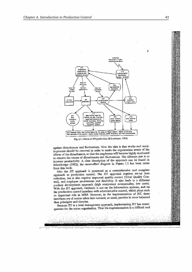
Chapter A. Introduction to Production Control 43

Chapter A. Introduction to Production Control 44
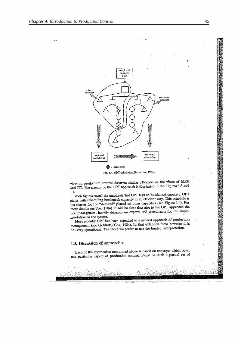
Chapter A. Introduction to Production Control 45

Chapter A. Introduction to Production Control 46

Chapter A. Introduction to Production Control 47
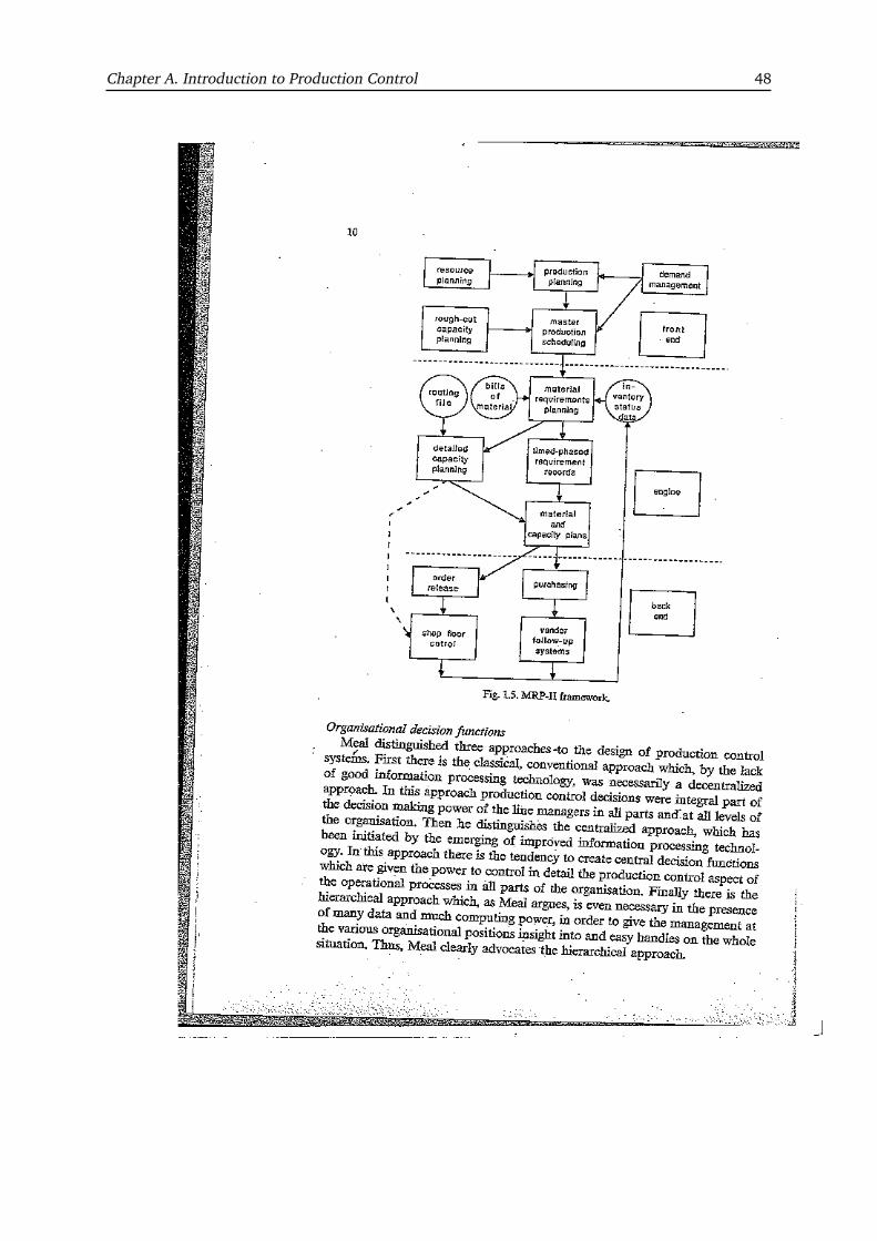
Chapter A. Introduction to Production Control 48

Chapter A. Introduction to Production Control 49

Chapter A. Introduction to Production Control 50

Chapter A. Introduction to Production Control 51
Chapter A. Introduction to Production Control 52
Chapter A. Introduction to Production Control 53
Chapter A. Introduction to Production Control 54

APPENDIX B
Production Units and Goods Flow Control
AcknowledgmentThis Appendix consists of Chapter 2 of the book Production Control: a Structural and Design OrientedApproach, written by J.W.M. Bertrand, J.C. Wortmann, and J. Wijngaard and is reproduced withtheir permission.
55

Chapter B. Production Units and Goods Flow Control 56
Chapter B. Production Units and Goods Flow Control 57

Chapter B. Production Units and Goods Flow Control 58
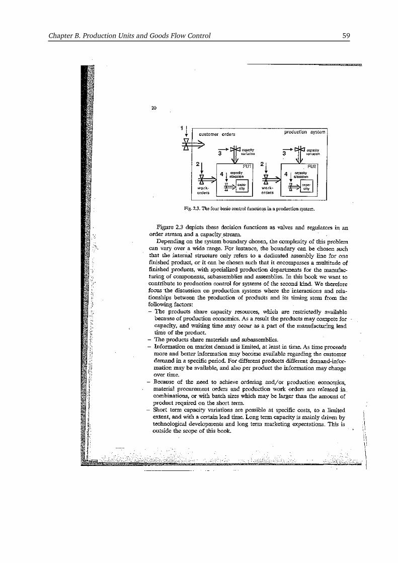
Chapter B. Production Units and Goods Flow Control 59
Chapter B. Production Units and Goods Flow Control 60
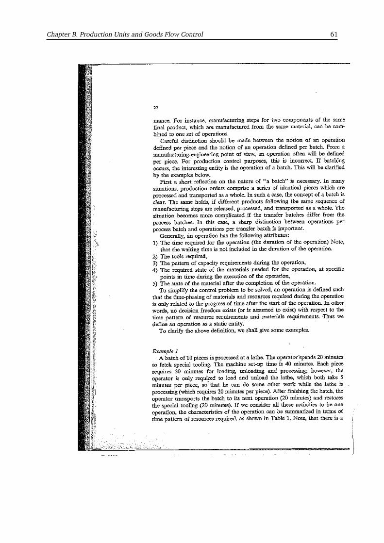
Chapter B. Production Units and Goods Flow Control 61

Chapter B. Production Units and Goods Flow Control 62

Chapter B. Production Units and Goods Flow Control 63

Chapter B. Production Units and Goods Flow Control 64

Chapter B. Production Units and Goods Flow Control 65
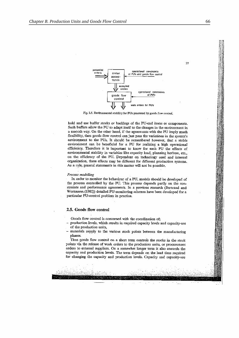
Chapter B. Production Units and Goods Flow Control 66
Chapter B. Production Units and Goods Flow Control 67

Chapter B. Production Units and Goods Flow Control 68

Chapter B. Production Units and Goods Flow Control 69
Chapter B. Production Units and Goods Flow Control 70
Chapter B. Production Units and Goods Flow Control 71
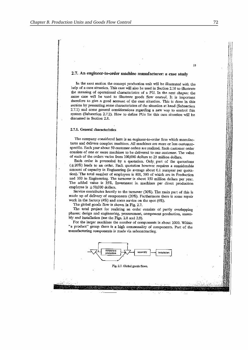
Chapter B. Production Units and Goods Flow Control 72
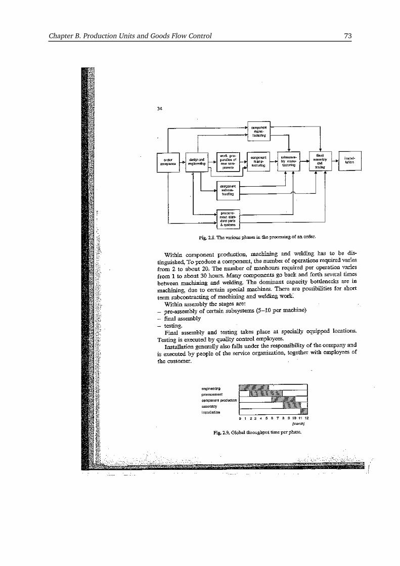
Chapter B. Production Units and Goods Flow Control 73

Chapter B. Production Units and Goods Flow Control 74

Chapter B. Production Units and Goods Flow Control 75
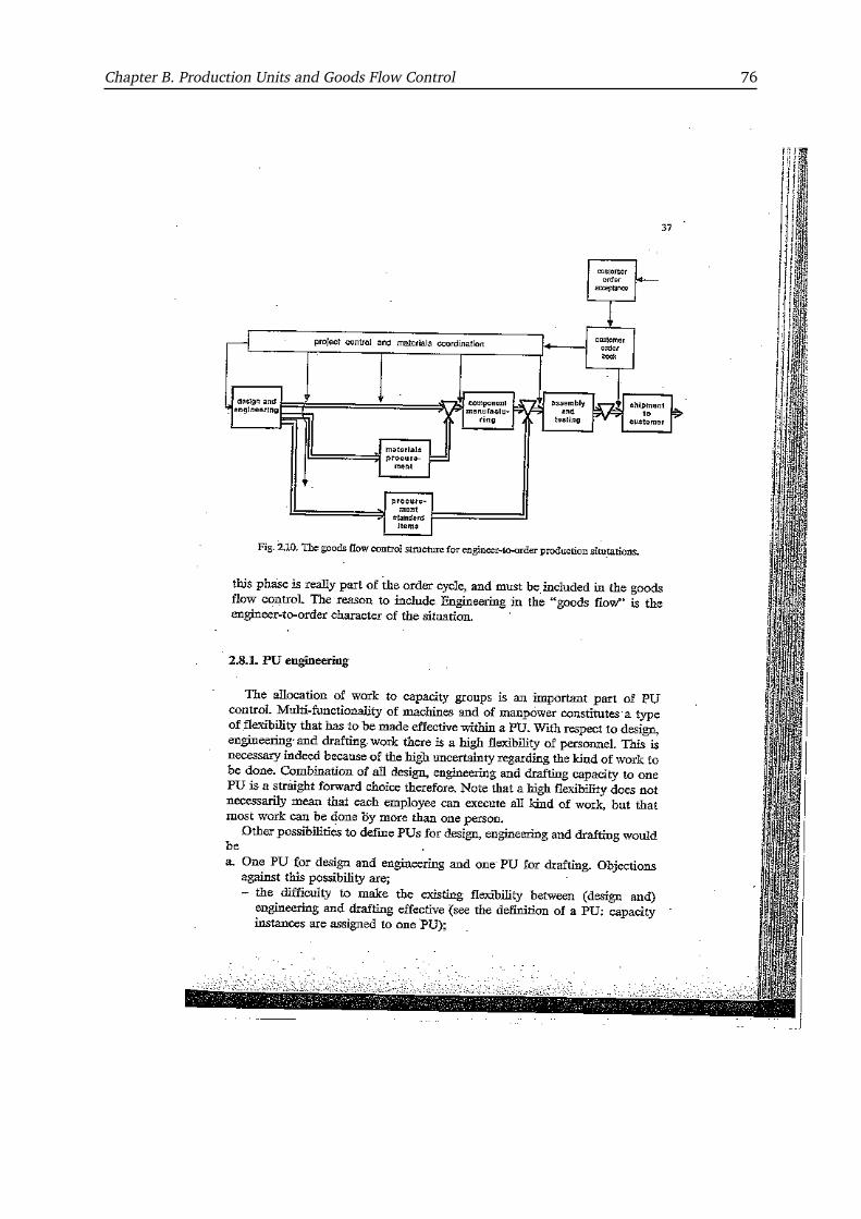
Chapter B. Production Units and Goods Flow Control 76

Chapter B. Production Units and Goods Flow Control 77
Chapter B. Production Units and Goods Flow Control 78
Chapter B. Production Units and Goods Flow Control 79

Chapter B. Production Units and Goods Flow Control 80

Chapter B. Production Units and Goods Flow Control 81
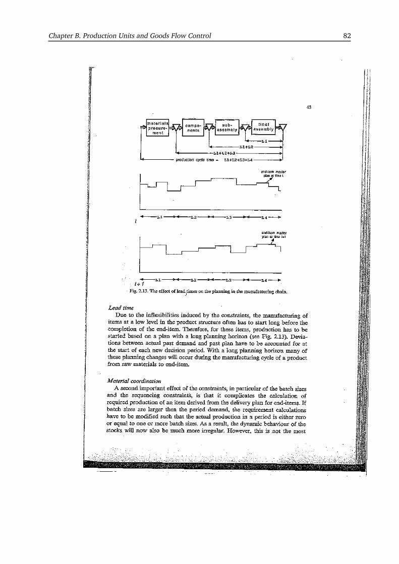
Chapter B. Production Units and Goods Flow Control 82

Chapter B. Production Units and Goods Flow Control 83
Chapter B. Production Units and Goods Flow Control 84

Chapter B. Production Units and Goods Flow Control 85
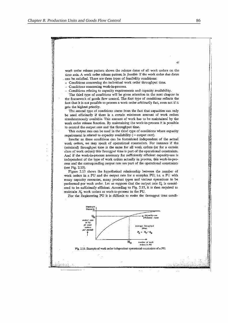
Chapter B. Production Units and Goods Flow Control 86
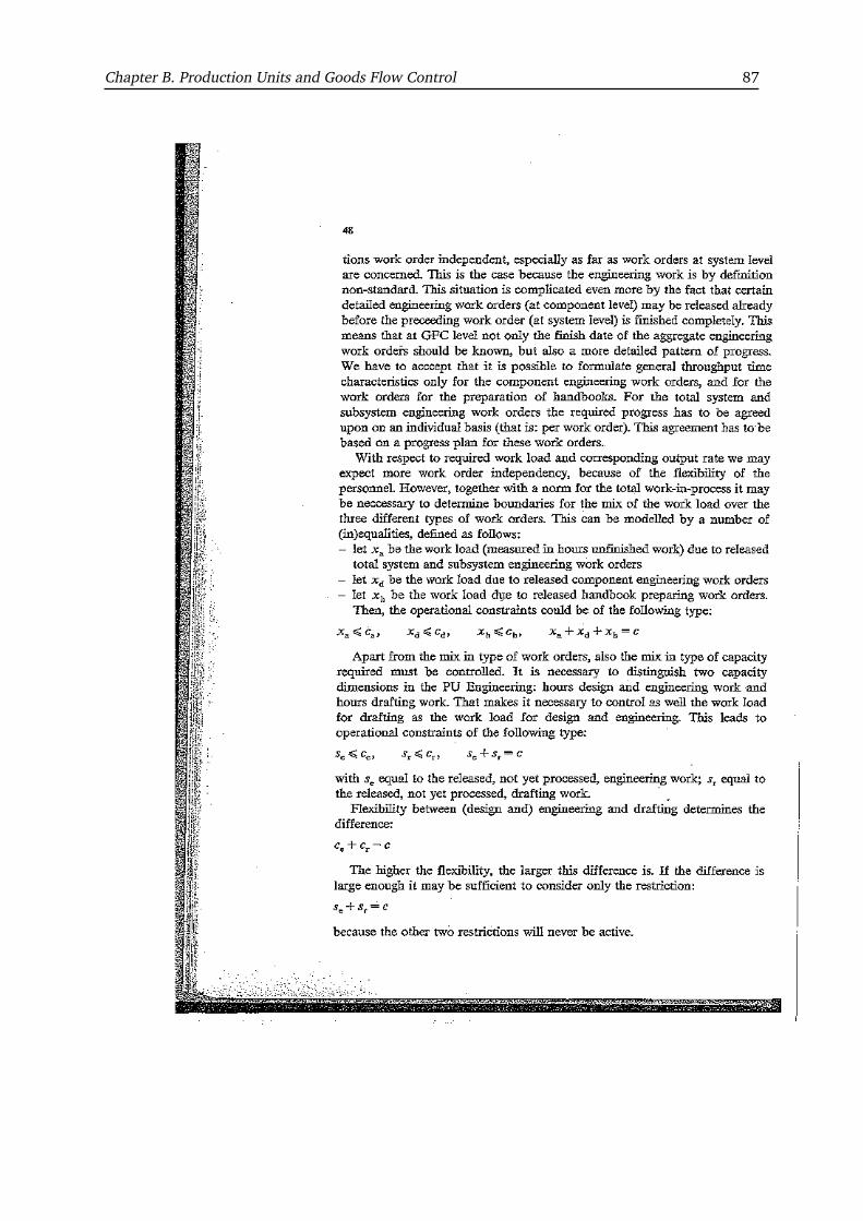
Chapter B. Production Units and Goods Flow Control 87
Chapter B. Production Units and Goods Flow Control 88
Chapter B. Production Units and Goods Flow Control 89
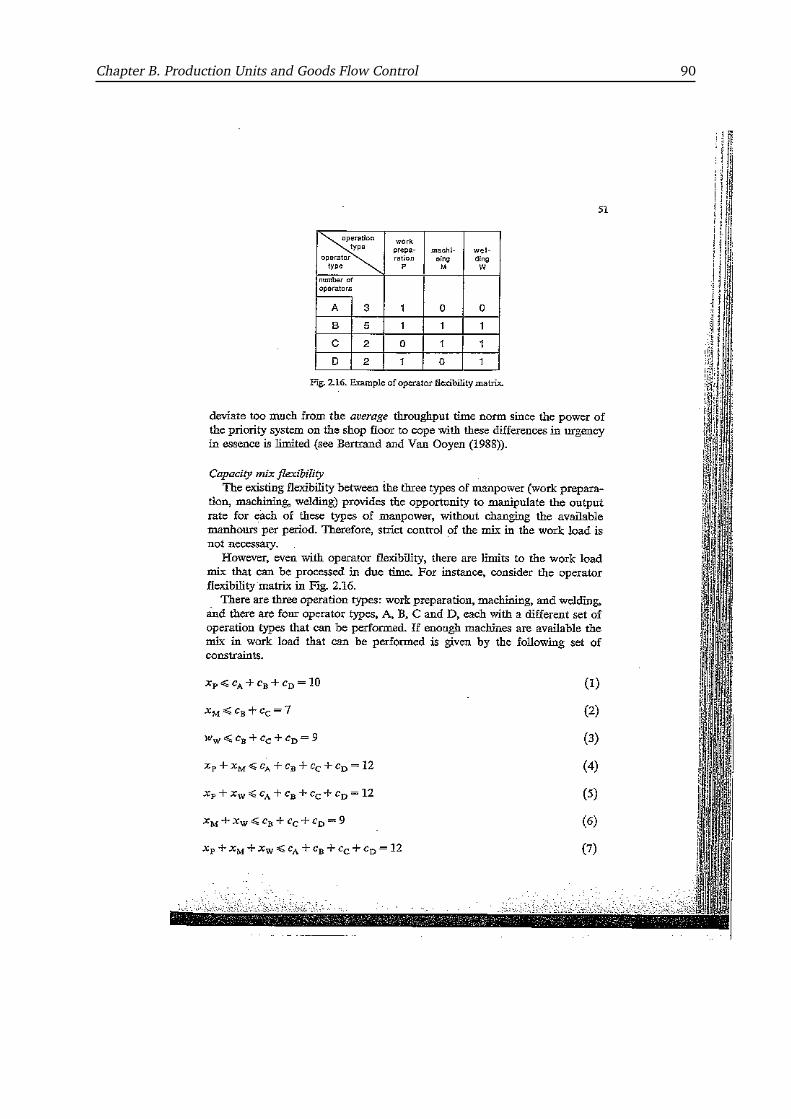
Chapter B. Production Units and Goods Flow Control 90

Chapter B. Production Units and Goods Flow Control 91
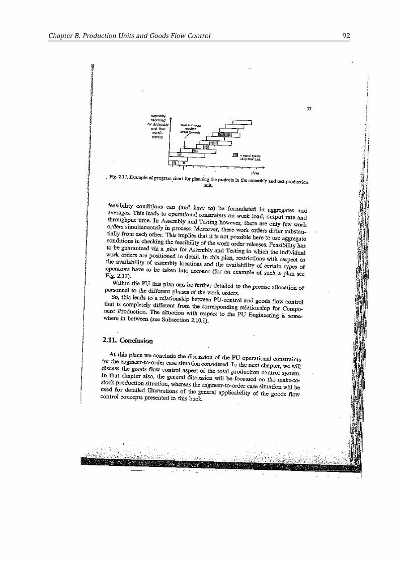
Chapter B. Production Units and Goods Flow Control 92

APPENDIX C
Goods Flow Control Structure
AcknowledgmentThis Appendix consists of Chapter 3 of the book Production Control: a Structural and Design OrientedApproach, written by J.W.M. Bertrand, J.C. Wortmann, and J. Wijngaard and is reproduced withtheir permission.
93

Chapter C. Goods Flow Control Structure 94

Chapter C. Goods Flow Control Structure 95

Chapter C. Goods Flow Control Structure 96
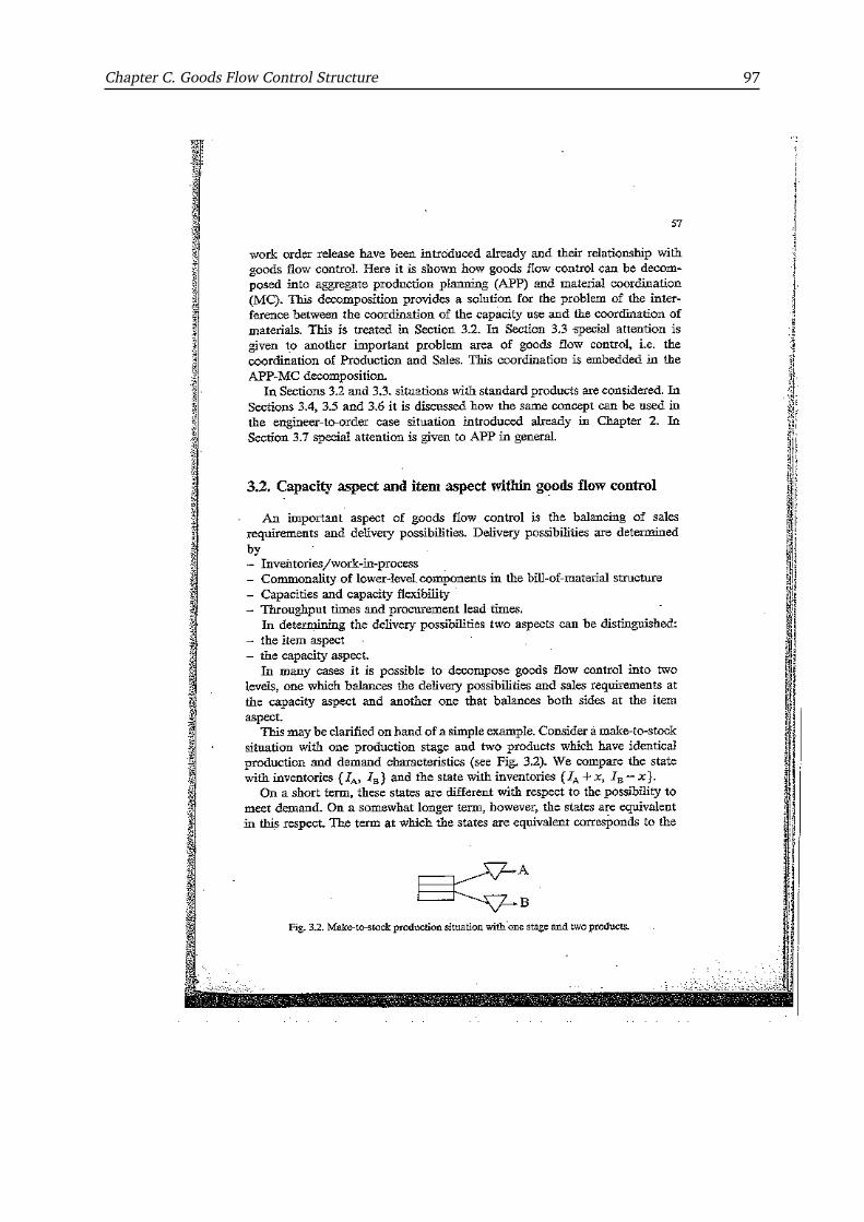
Chapter C. Goods Flow Control Structure 97

Chapter C. Goods Flow Control Structure 98

Chapter C. Goods Flow Control Structure 99
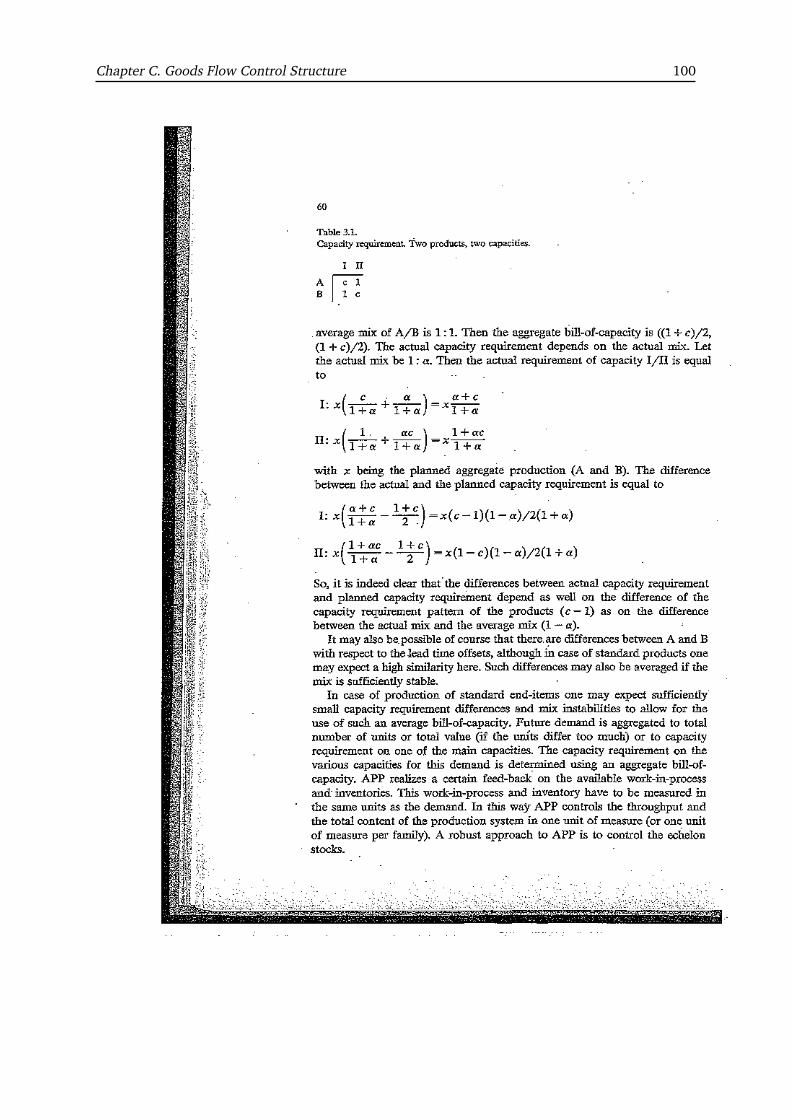
Chapter C. Goods Flow Control Structure 100
Chapter C. Goods Flow Control Structure 101
Chapter C. Goods Flow Control Structure 102

Chapter C. Goods Flow Control Structure 103
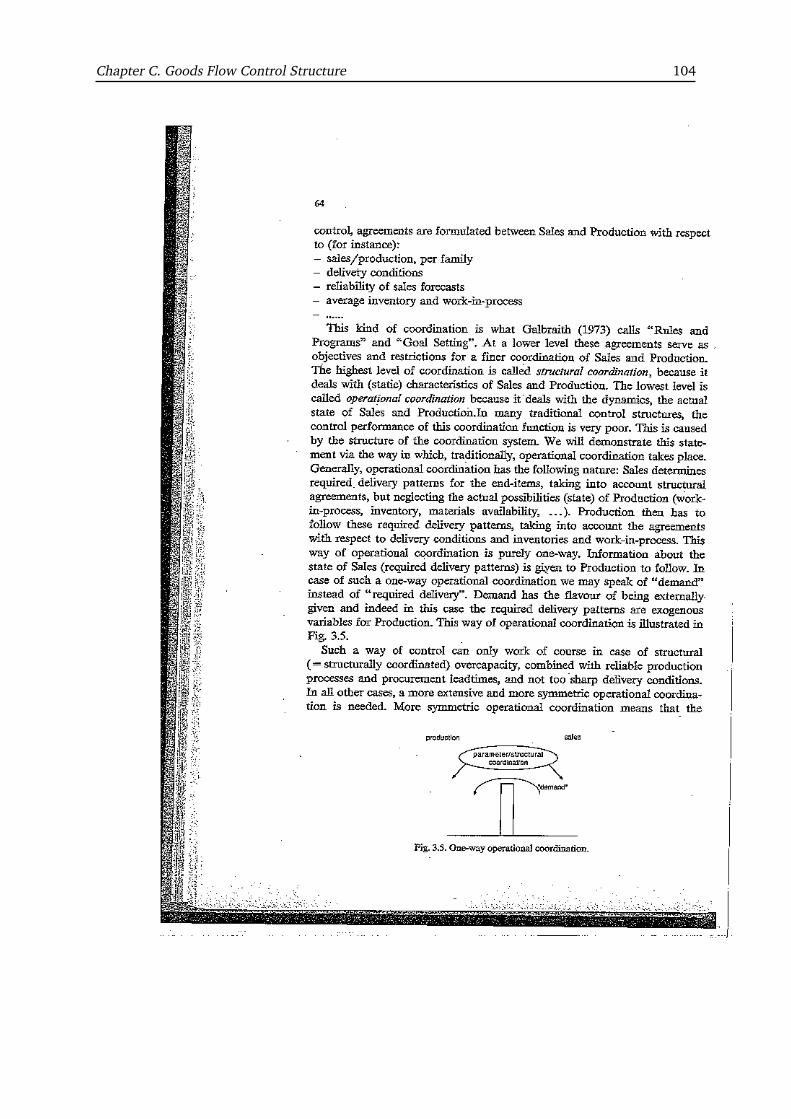
Chapter C. Goods Flow Control Structure 104

Chapter C. Goods Flow Control Structure 105
Chapter C. Goods Flow Control Structure 106
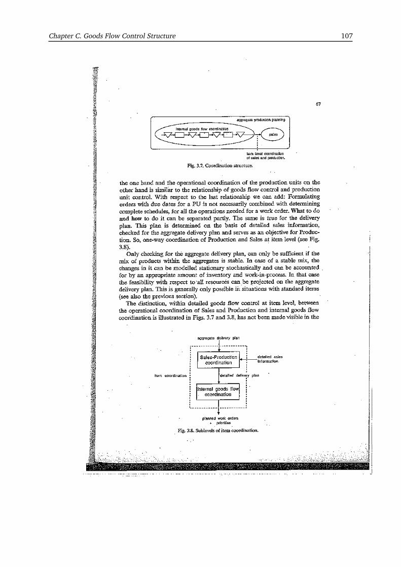
Chapter C. Goods Flow Control Structure 107
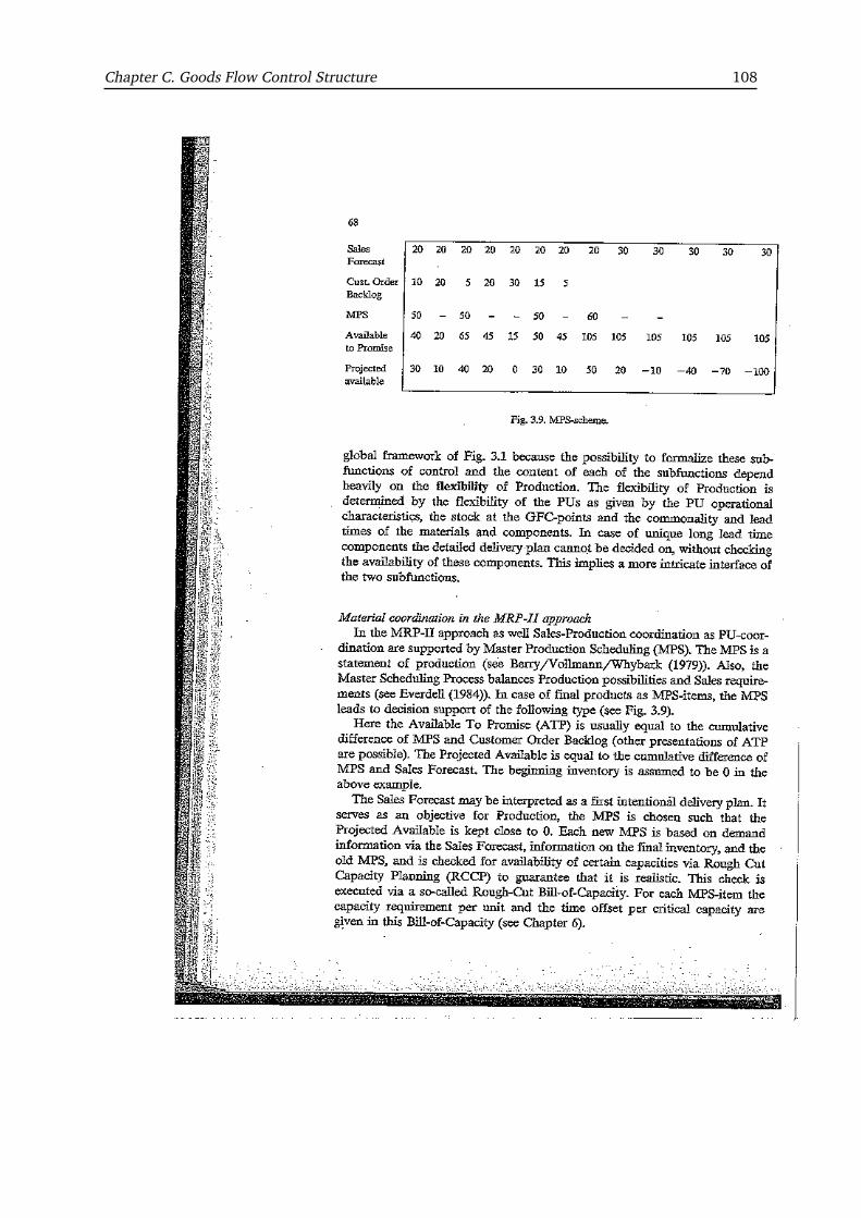
Chapter C. Goods Flow Control Structure 108
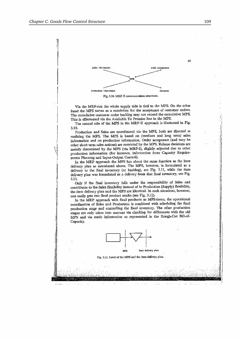
Chapter C. Goods Flow Control Structure 109
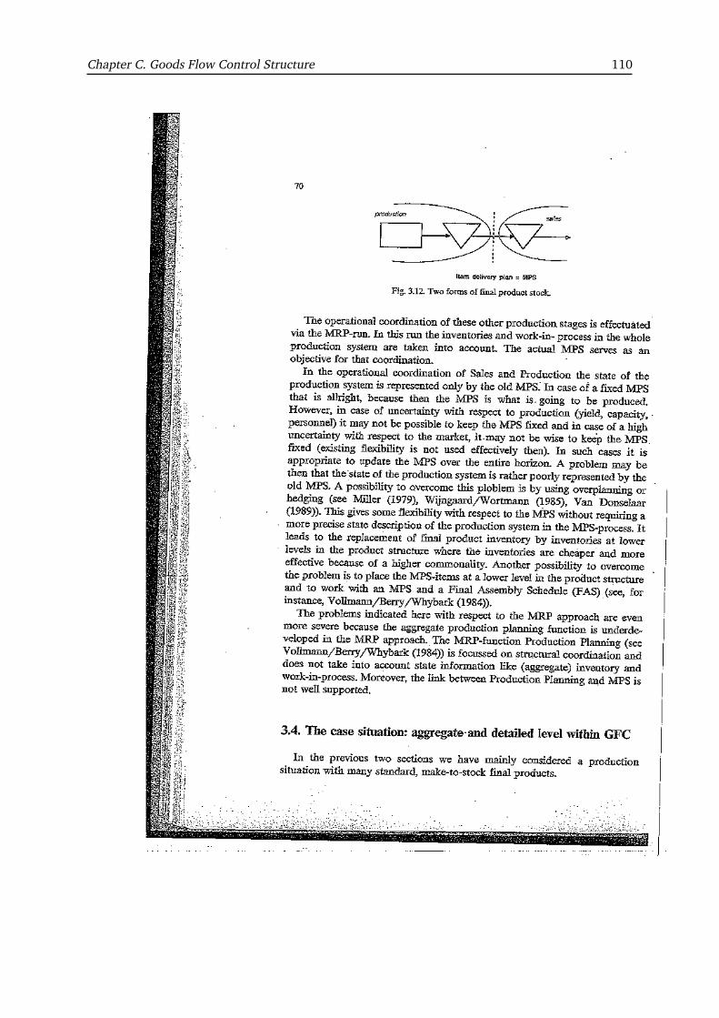
Chapter C. Goods Flow Control Structure 110
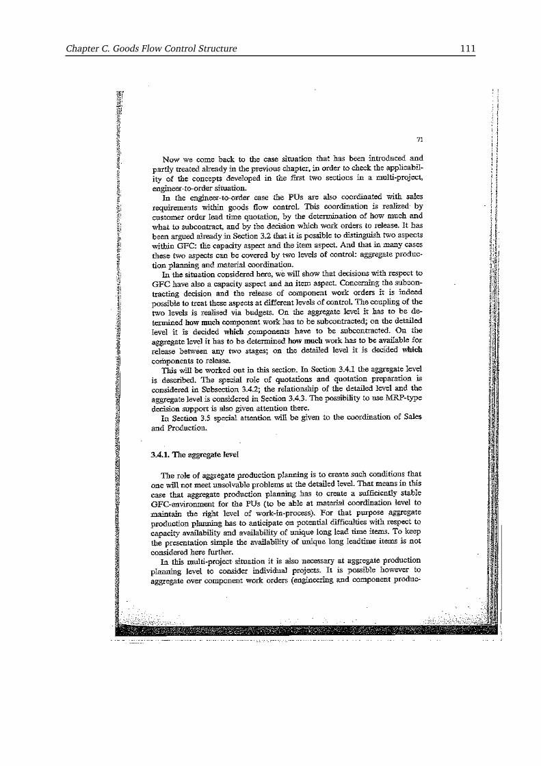
Chapter C. Goods Flow Control Structure 111
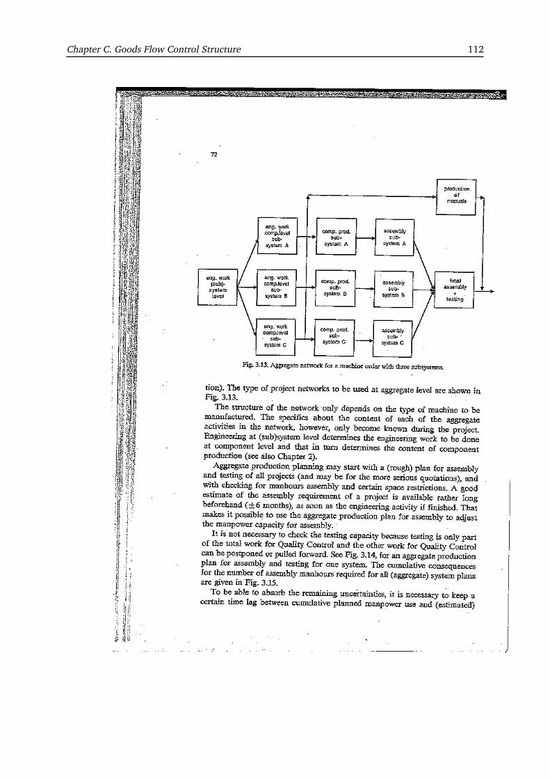
Chapter C. Goods Flow Control Structure 112

Chapter C. Goods Flow Control Structure 113
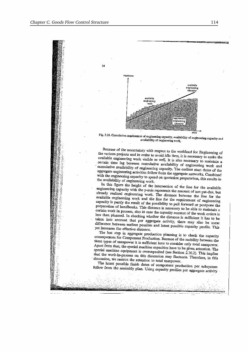
Chapter C. Goods Flow Control Structure 114
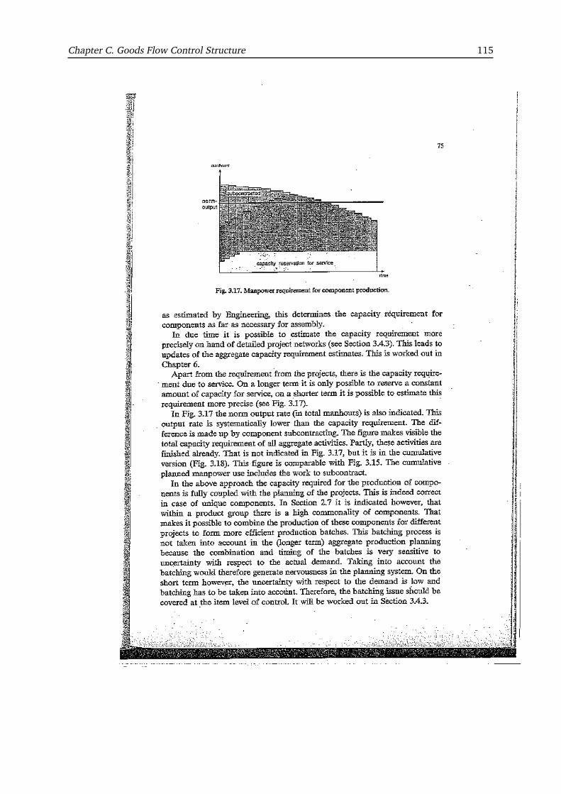
Chapter C. Goods Flow Control Structure 115

Chapter C. Goods Flow Control Structure 116
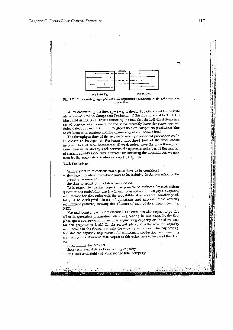
Chapter C. Goods Flow Control Structure 117
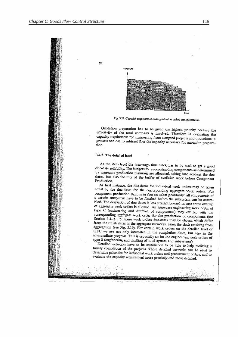
Chapter C. Goods Flow Control Structure 118

Chapter C. Goods Flow Control Structure 119

Chapter C. Goods Flow Control Structure 120
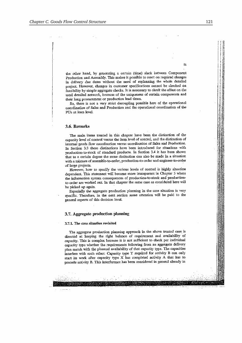
Chapter C. Goods Flow Control Structure 121

Chapter C. Goods Flow Control Structure 122
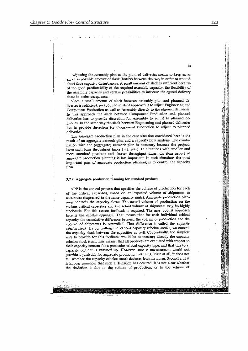
Chapter C. Goods Flow Control Structure 123

Chapter C. Goods Flow Control Structure 124
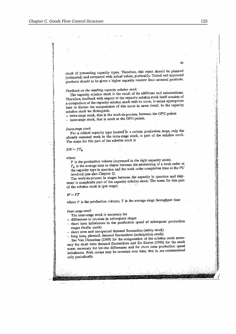
Chapter C. Goods Flow Control Structure 125
Chapter C. Goods Flow Control Structure 126

Chapter C. Goods Flow Control Structure 127

APPENDIX D
Production Control in a Complex Component Manufacturing Firm
AcknowledgmentThis Appendix consists of Chapter 8 of the book Production Control: a Structural and Design OrientedApproach, written by J.W.M. Bertrand, J.C. Wortmann, and J. Wijngaard and is reproduced withtheir permission.
128
Chapter D. Production Control in a Complex Component Manufacturing Firm 129
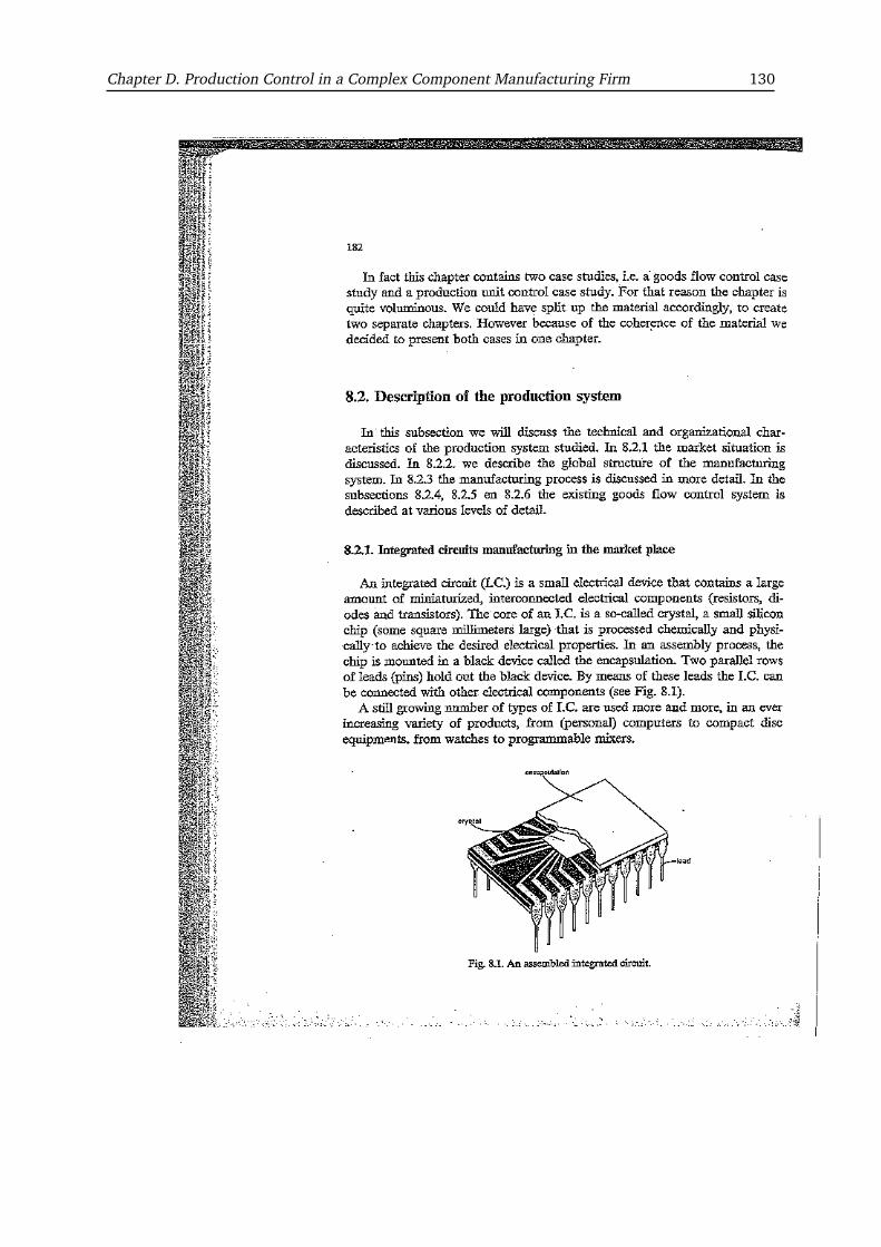
Chapter D. Production Control in a Complex Component Manufacturing Firm 130
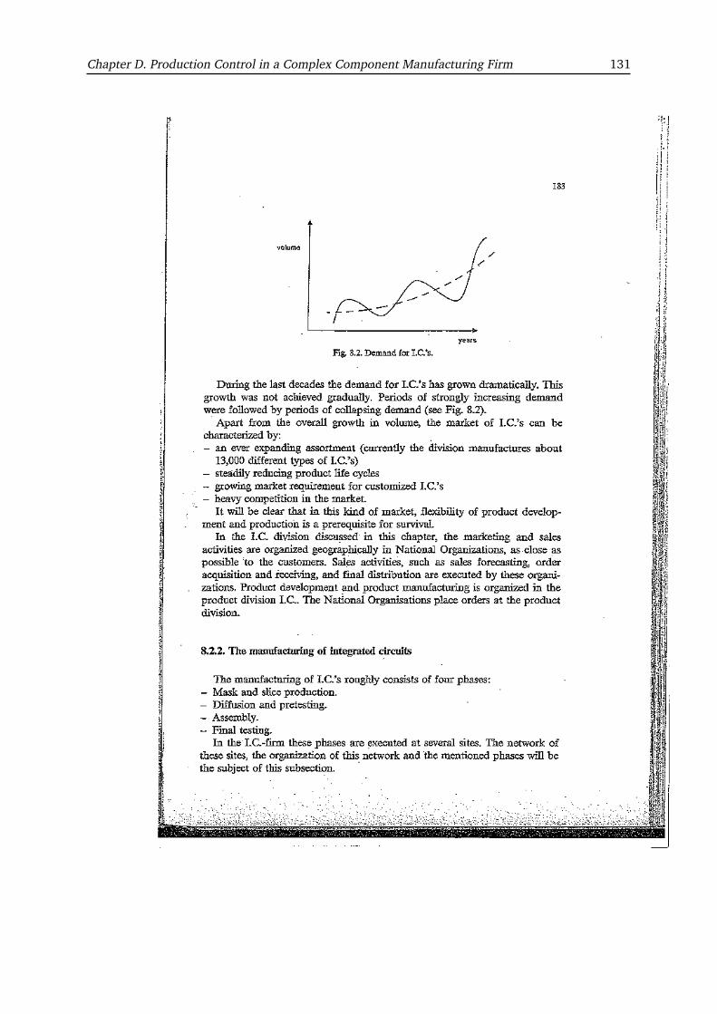
Chapter D. Production Control in a Complex Component Manufacturing Firm 131

Chapter D. Production Control in a Complex Component Manufacturing Firm 132

Chapter D. Production Control in a Complex Component Manufacturing Firm 133

Chapter D. Production Control in a Complex Component Manufacturing Firm 134

Chapter D. Production Control in a Complex Component Manufacturing Firm 135

Chapter D. Production Control in a Complex Component Manufacturing Firm 136

Chapter D. Production Control in a Complex Component Manufacturing Firm 137
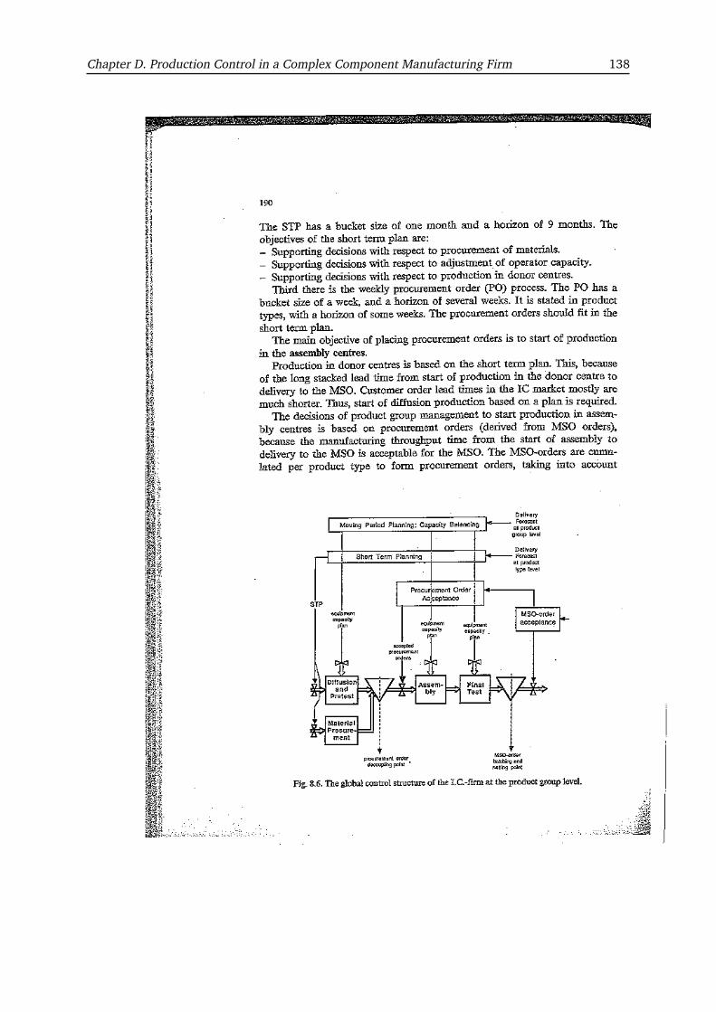
Chapter D. Production Control in a Complex Component Manufacturing Firm 138

Chapter D. Production Control in a Complex Component Manufacturing Firm 139
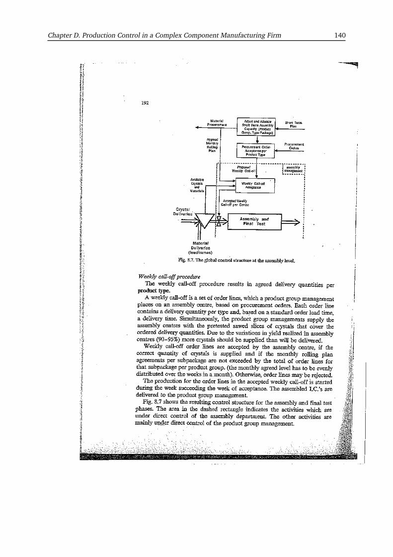
Chapter D. Production Control in a Complex Component Manufacturing Firm 140
Chapter D. Production Control in a Complex Component Manufacturing Firm 141
Chapter D. Production Control in a Complex Component Manufacturing Firm 142

Chapter D. Production Control in a Complex Component Manufacturing Firm 143
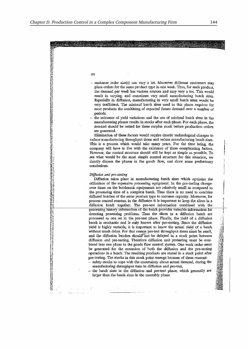
Chapter D. Production Control in a Complex Component Manufacturing Firm 144

Chapter D. Production Control in a Complex Component Manufacturing Firm 145

Chapter D. Production Control in a Complex Component Manufacturing Firm 146
Chapter D. Production Control in a Complex Component Manufacturing Firm 147

Chapter D. Production Control in a Complex Component Manufacturing Firm 148

Chapter D. Production Control in a Complex Component Manufacturing Firm 149

Chapter D. Production Control in a Complex Component Manufacturing Firm 150

Chapter D. Production Control in a Complex Component Manufacturing Firm 151

Chapter D. Production Control in a Complex Component Manufacturing Firm 152

Chapter D. Production Control in a Complex Component Manufacturing Firm 153

Chapter D. Production Control in a Complex Component Manufacturing Firm 154
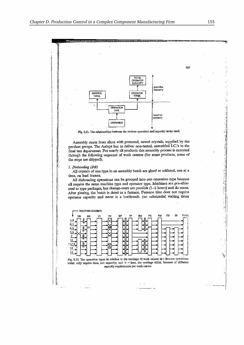
Chapter D. Production Control in a Complex Component Manufacturing Firm 155

Chapter D. Production Control in a Complex Component Manufacturing Firm 156

Chapter D. Production Control in a Complex Component Manufacturing Firm 157

Chapter D. Production Control in a Complex Component Manufacturing Firm 158

Chapter D. Production Control in a Complex Component Manufacturing Firm 159
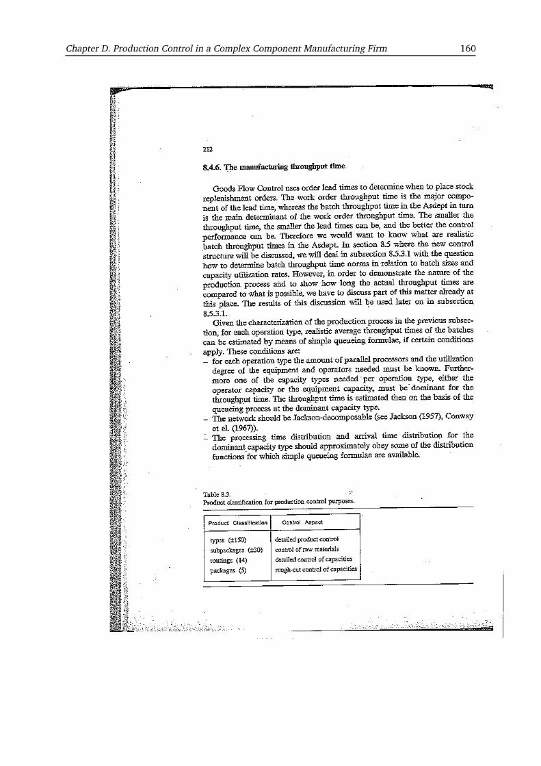
Chapter D. Production Control in a Complex Component Manufacturing Firm 160
Chapter D. Production Control in a Complex Component Manufacturing Firm 161
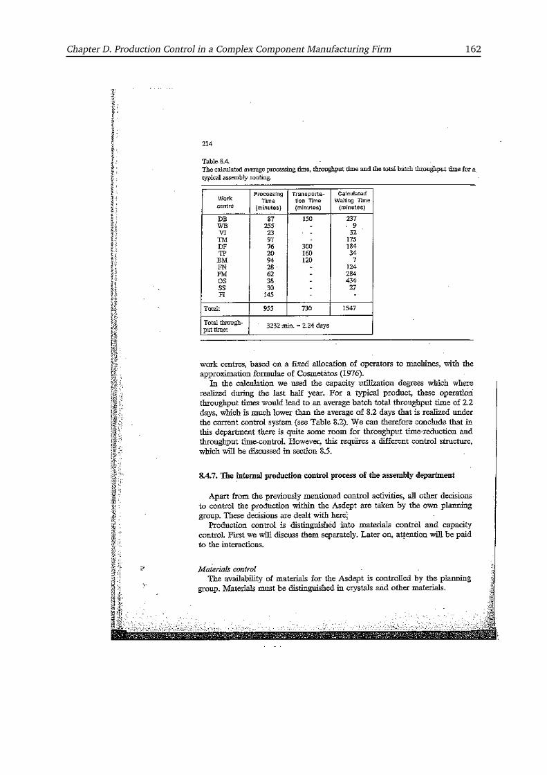
Chapter D. Production Control in a Complex Component Manufacturing Firm 162
Chapter D. Production Control in a Complex Component Manufacturing Firm 163
Chapter D. Production Control in a Complex Component Manufacturing Firm 164

Chapter D. Production Control in a Complex Component Manufacturing Firm 165
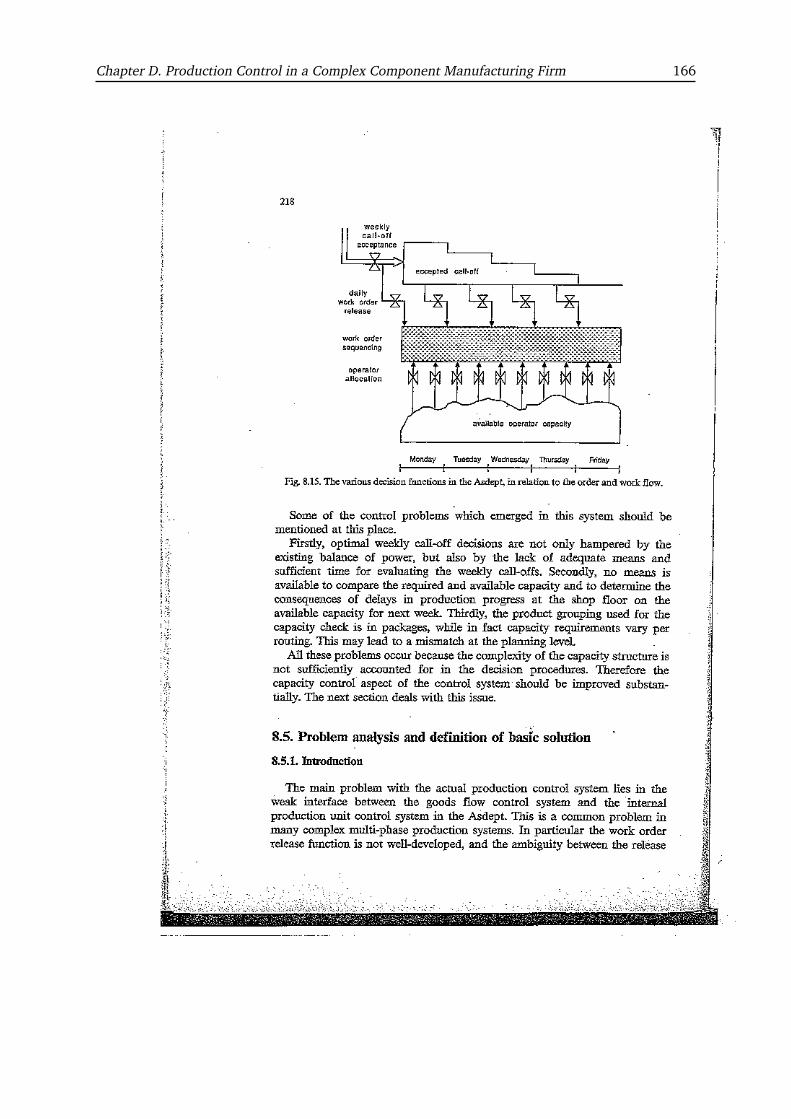
Chapter D. Production Control in a Complex Component Manufacturing Firm 166
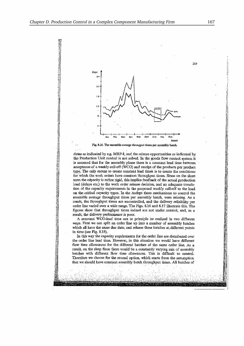
Chapter D. Production Control in a Complex Component Manufacturing Firm 167

Chapter D. Production Control in a Complex Component Manufacturing Firm 168
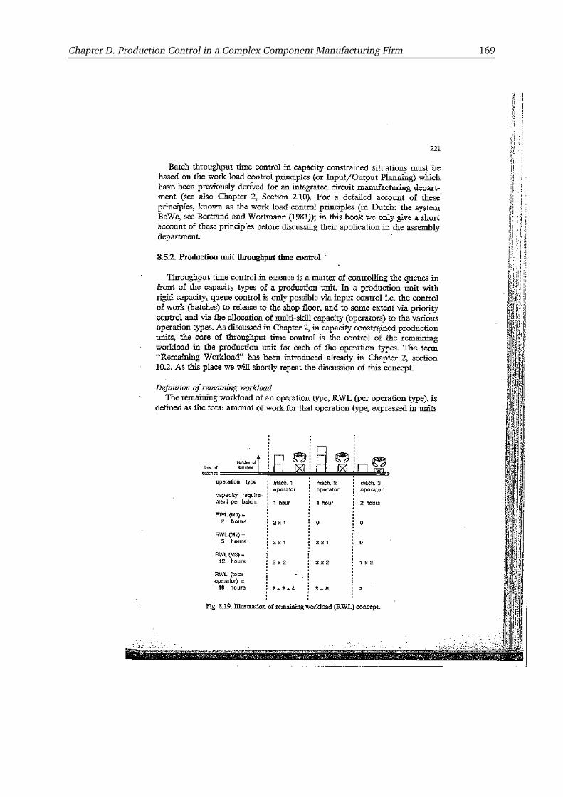
Chapter D. Production Control in a Complex Component Manufacturing Firm 169
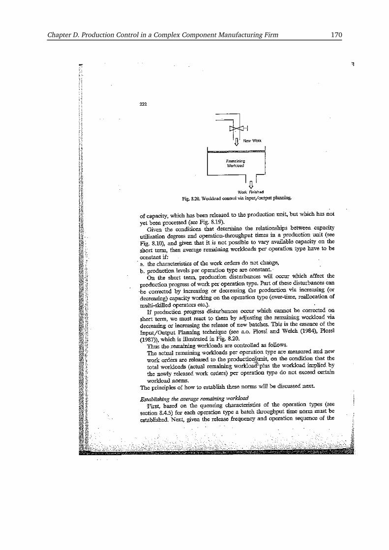
Chapter D. Production Control in a Complex Component Manufacturing Firm 170
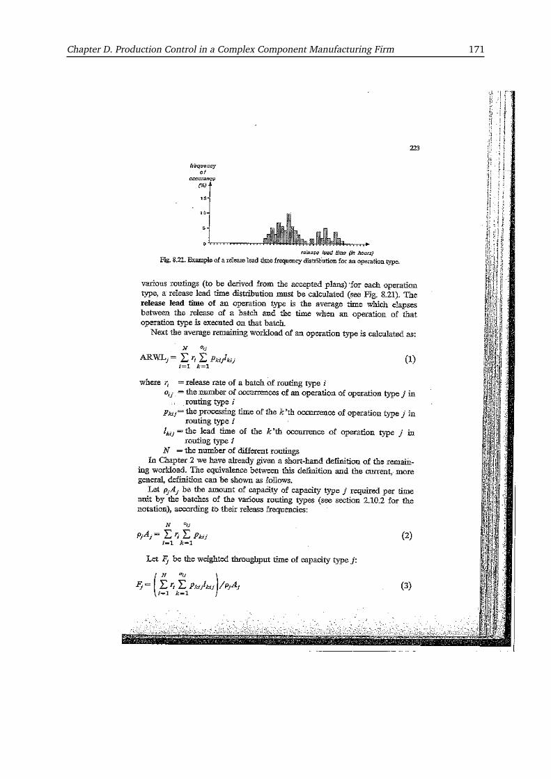
Chapter D. Production Control in a Complex Component Manufacturing Firm 171

Chapter D. Production Control in a Complex Component Manufacturing Firm 172
Chapter D. Production Control in a Complex Component Manufacturing Firm 173
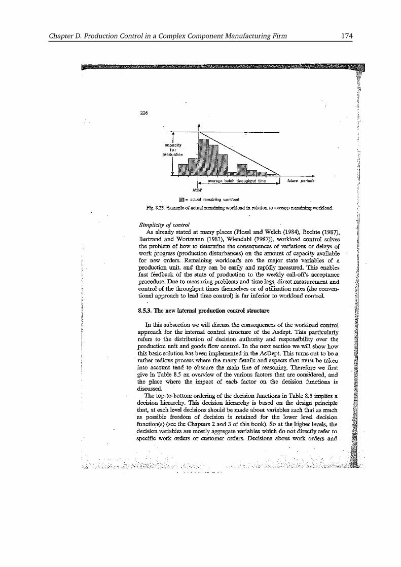
Chapter D. Production Control in a Complex Component Manufacturing Firm 174

Chapter D. Production Control in a Complex Component Manufacturing Firm 175
Chapter D. Production Control in a Complex Component Manufacturing Firm 176
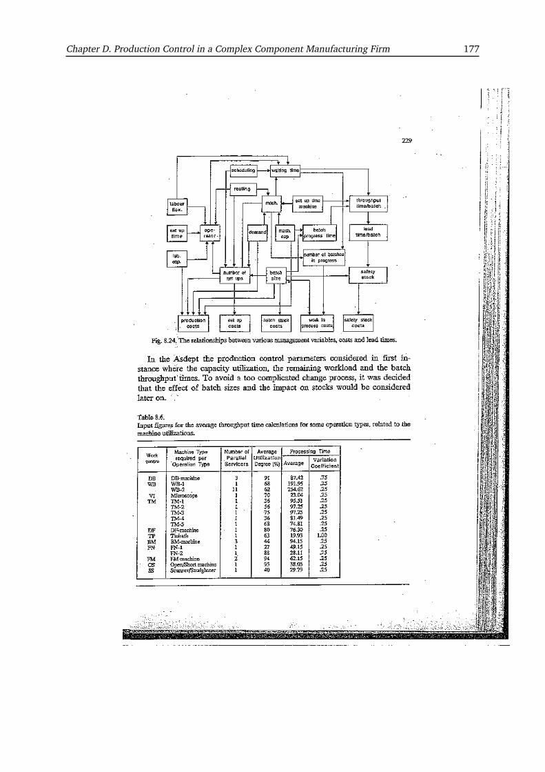
Chapter D. Production Control in a Complex Component Manufacturing Firm 177

Chapter D. Production Control in a Complex Component Manufacturing Firm 178

Chapter D. Production Control in a Complex Component Manufacturing Firm 179

Chapter D. Production Control in a Complex Component Manufacturing Firm 180

Chapter D. Production Control in a Complex Component Manufacturing Firm 181
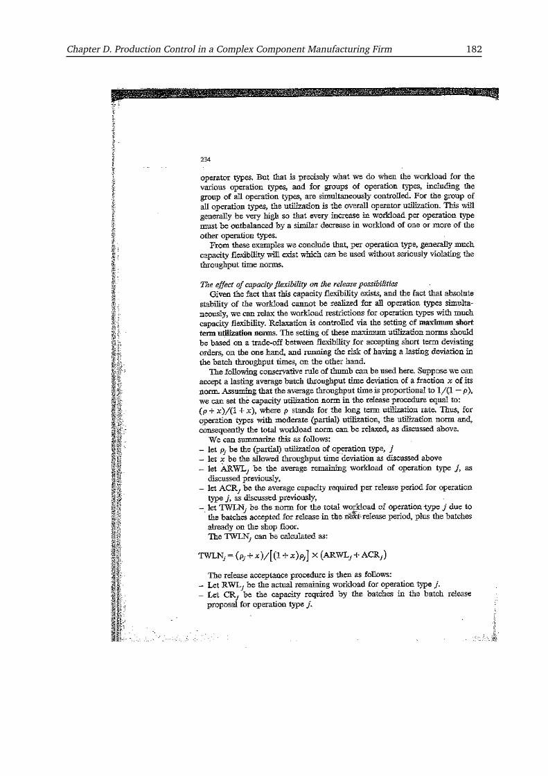
Chapter D. Production Control in a Complex Component Manufacturing Firm 182

Chapter D. Production Control in a Complex Component Manufacturing Firm 183

Chapter D. Production Control in a Complex Component Manufacturing Firm 184

Chapter D. Production Control in a Complex Component Manufacturing Firm 185
Chapter D. Production Control in a Complex Component Manufacturing Firm 186

Bibliography
Adam, N. R., Bertrand, J. W. M., & Surkis, J. (1987). Priority assignment procedures in multi-levelassembly job shops. IIE Transactions, 19, 311-328.
Allen, T. (1987). Managing the flow of technology. Cambridge, Mass.: Harvard University Press.
Altiok, T. (1997). Performance analysis of manufacturing systems. Berlin: Springer Verlag.
Anthony, R. N. (1965). Planning and control systems: A framework for analysis. Harvard UniversityPress.
Axsäter, S. (1981). Aggregation of product data for hierarchical production planning. OperationsResearch, 29(4), 744–756.
Axsäter, S. (1986). On the feasibility of aggregate production plans. Operations Research, 34(5),796–800.
Axsäter, S., & Jönsson, H. (1984). Aggregation and disaggregation in hierarchical productionplanning. European Journal of Operational Research, 17, 338-350.
Baker, K. R., & Bertand, J. W. M. (1981). An investigation of due date assignment rules withconstraint tightness. Journal of Operations Management, 1, 109-120.
Baldwin, C. Y., & Clarck, K. B. (2000). Design rules, volume 1: The power of modularity. Cambridge,Mass.: The MIT Press.
Baskett, F., Chandy, K. M., Muntz, R. R., & Palacios, F. G. (1975). Open, closed, and mixed networksof queues with different classes of customers. Journal of the ACM (JACM), 22(2), 260.
Bechte, W. (1987). Theory and practice of load-oriented manufacturing control. InternationalJournal of Production Control, 26, 375-396.
Bemelmans, R. P. H. G. (1986). The capacity aspect of inventories. Springer.
Bertand, J. W. M., & Van Ooijen, H. P. G. (1988). The control of categories of work order flow rates.(Working Paper Bdk/KBS/88, Eindhoven University of Technology)
Bertrand, J. W. M. (1985). Multi-product optimal batch sizes with in-process inventories and multiwork centers. IIE Transactions, 17, 157-163.
Bertrand, J. W. M., & Wortmann, J. C. (1981). Production control and information systems forcomponent manufacturing shops (Vol. 1). Amsterdam: Elsevier.
Bertrand, J. W. M., Wortmann, J. C., & Wijngaard, J. (1990). Production control: A structural anddesign oriented approach (Vol. 11). Amsterdam: Elsevier.
Bitran, G. R., Haas, E. A., & Hax, A. C. (1981). Hierarchical production planning: A single stagesystem. Operations Research, 29(4), 717–743.
Bitran, G. R., Haas, E. A., & Hax, A. C. (1982). Hierarchical production planning: A two-stagesystem. Operations Research, 30(2), 232–251.
Bitran, G. R., & Hax, A. C. (1977). On the design of hierarchical production planning systems.Decision Sciences, 8(1), 28-55.
187

BIBLIOGRAPHY 188
Bitran, G. R., & Tirupati, D. (1988). Multiproduct queueing networks with deterministic routing:Decomposition approach and the notion of interference. Management Science, 34(1), 75–100.
Bitran, G. R., & Tirupati, D. (1993). Hierarchical production planning. In (Vol. 4, p. 523-568).North-Holland.
Brown, R. G. (1977). Materials management systems. Wiley.
Burbidge. (1971). The principles of production control (Third ed.). Macdonald and Evans.
Buzacott, J. A. (1989). Queueing models of kanban and mrp controlled production systems. Engi-neering Costs and Production Economics, 17, 3-20.
Buzacott, J. A., & Shanthikumar, J. G. (1993). Stochastic models of manufacturing systems. Prentice-Hall.
Byrne, M. D., & Bakir, M. A. (1999). Production planning using a hybrid simulation–analyticalapproach. International Journal of Production Economics, 59(1-3), 305–311.
Byrne, M. D., & Hossain, M. M. (2005). Production planning: An improved hybrid approach.International Journal of Production Economics, 93, 225–229.
Ciarallo, F. W., Akella, R., & Morton, T. E. (1994). A periodic review, production planning-modelwith uncertain capacity and uncertaint demand - optimality of extended myopic policies. Man-agement Science, 40(3), 320–332.
Conway, R. W., Maxwell, W. L., & Miller, L. W. (1967). Theory of scheduling. Addison-Wesley.
Cosmetatos, G. P. (1976). Some approximate equilibrium results for the multi-server queue (m/g/r).Operations Research Quarterly, 27, 615-620.
Dauzère-Pérès, S., & Lasserre, J. B. (1994). Integration of lotsizing and scheduling decisions in ajob-shop. European Journal of Operational Research, 75, 413-426.
de Kok, A. G., & Fransoo, J. C. (2003). Planning supply chain operations: definition and comparisonof planning concepts. Handbooks in operations research and management science, 11, 597–676.
De Koster, M. B. M. (1989). Capacity oriented analysis and design of production systems. Springer.
Durlinger, P. P. J. (1989). Estimating waiting times in dual constraint production systems (Tech.Rep.). Eindhoven University Research Report, TUE/BDK/KBS/01.
Durlinger, P. P. J., & Bertrand, J. W. M. (1983). Balancing logistics related costs in multi-phaseproduction systems (Tech. Rep.). Eindhoven University Research Report, TUE/BMK/KBS/09.
Erlang, A. K. (1918). Solutions of some problems in the theory of probabilities of significance inautomatic telephone exchanges. The Post Office Electrical Engineers’ Journal, 10, 189-197.
Everdell. (1984). Master scheduling. APICS Training Aid. APICS.
Fleischmann, B., & Meyr, H. (2002). De kok, a.g. and s.c. graves (eds.) supply chain management.In (chap. Planning hierarchy, modeling, and advanced planning systems). Amsteram: North-Holland.
Frein, Y., Di Mascola, M., & Dallery, Y. (1995). On the design of generalized kanban control systems.International Journal of Operations and Production Management, 15(9), 158-184.
Fryer, J. S. (1973). Operating policies in multi echelon dual-constraint job shops. ManagementScience, 19, 1001-1012.

BIBLIOGRAPHY 189
Fryer, J. S. (1974). Labor flexbility in multi echelon dual-constaint job shops. Management Science,20, 1073-1080.
Gailbraith, J. R. (1973). Designing complex organzations. Addison-Wesley.
Gelders, L. F., & van Wassenhove, L. N. (1982). Hierarchical integration in production planning:Theory and practice. Journal of Operations Management, 3(1), 27–35.
Gershwin, S. B. (1994). Manufacturing systems engineering. Engleweed Cliffs: Prentice Hall.
Graves, S. C., Rinnooy Kan, A. H. G., & Zipkin, P. H. (1993). Logistics of production and inventory(Vol. 4). Amsterdam: Elsevier.
Harris, F. (1913). How many parts to make at once. Factory, The Magazine of Management, 10,135-136.
Hax, A. C., & Candea, D. (1984). Production and inventory management (Vol. 1). Prentice-HallEnglewood Cliffs, NJ.
Hax, A. C., & Meal, H. C. (1973). Hierarchical integration of production planning and scheduling.(Tech. Rep.). MIT, Sloan School of Management.
Henig, M., & Gerchak, Y. (1990). The structure of peridodic review policies in the presence ofrandom yield. Operations Research, 38(4), 634–643.
Hopp, W. J., & Spearman, M. L. (2000). Factory physics (Second ed.). Boston: McGraw-Hill.
Hung, Y. F., & Leachman, R. C. (1996). A production planning methodology for semiconductormanufacturingbased on iterative simulation and linear programming calculations. IEEE Transac-tions on Semiconductor Manufacturing, 9(2), 257–269.
Irdem, D. F., Kacar, N. B., & Uzsoy, R. (2010). An exploratory analysis of two iterative linearprogrammingsimulation approaches for production planning. Semiconductor Manufacturing,IEEE Transactions on Semiconductor Manufacturing, 23(3), 442–455.
Jackson, J. R. (1957). Networks of waiting lines. Operations Research, 5(4), 518–521.
Jenkins, R. V. (1987). Words, images, artifacts and sound: Documents for the history of technology.British Journal of History of Science, 20, 39-57.
Kanet, J. J., & Hayya, J. C. (1982). Priority dispatching with operation due dates in a job shop.Journal of Operations Management, 2, 167-175.
Kanet, J. J., & Sridharan, S. V. (1998). The value of using scheduling information in planningmaterial requirements. Decision Sciences, 29(2), 479-497.
Karmaker, U. S. (1987). Lot-sizes, manufacturing lead times and in-process inventories. Manage-ment Science, 33, 409-418.
Kim, B., & Kim, S. (2001). Extended model for a hybrid production planning approach. InternationalJournal of Production Economics, 73(2), 165–173.
Kleinrock, L. (1975). Queueing systems, volume i: theory. Wiley Interscience.
Lawrence, S. R. (1997). Heuristic, optimal, static, and dynamic schedules when processing timesare uncertain. Journal of Operations Management, 15(1), 71-82.
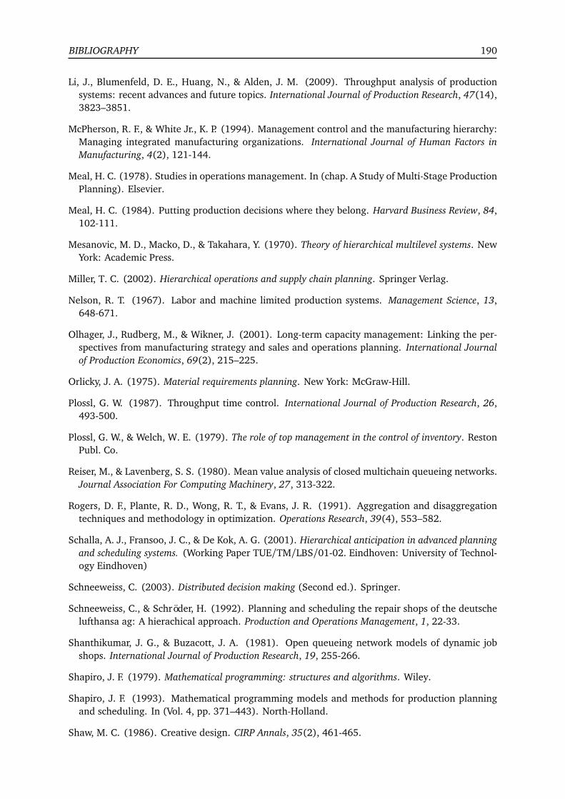
BIBLIOGRAPHY 190
Li, J., Blumenfeld, D. E., Huang, N., & Alden, J. M. (2009). Throughput analysis of productionsystems: recent advances and future topics. International Journal of Production Research, 47(14),3823–3851.
McPherson, R. F., & White Jr., K. P. (1994). Management control and the manufacturing hierarchy:Managing integrated manufacturing organizations. International Journal of Human Factors inManufacturing, 4(2), 121-144.
Meal, H. C. (1978). Studies in operations management. In (chap. A Study of Multi-Stage ProductionPlanning). Elsevier.
Meal, H. C. (1984). Putting production decisions where they belong. Harvard Business Review, 84,102-111.
Mesanovic, M. D., Macko, D., & Takahara, Y. (1970). Theory of hierarchical multilevel systems. NewYork: Academic Press.
Miller, T. C. (2002). Hierarchical operations and supply chain planning. Springer Verlag.
Nelson, R. T. (1967). Labor and machine limited production systems. Management Science, 13,648-671.
Olhager, J., Rudberg, M., & Wikner, J. (2001). Long-term capacity management: Linking the per-spectives from manufacturing strategy and sales and operations planning. International Journalof Production Economics, 69(2), 215–225.
Orlicky, J. A. (1975). Material requirements planning. New York: McGraw-Hill.
Plossl, G. W. (1987). Throughput time control. International Journal of Production Research, 26,493-500.
Plossl, G. W., & Welch, W. E. (1979). The role of top management in the control of inventory. RestonPubl. Co.
Reiser, M., & Lavenberg, S. S. (1980). Mean value analysis of closed multichain queueing networks.Journal Association For Computing Machinery, 27, 313-322.
Rogers, D. F., Plante, R. D., Wong, R. T., & Evans, J. R. (1991). Aggregation and disaggregationtechniques and methodology in optimization. Operations Research, 39(4), 553–582.
Schalla, A. J., Fransoo, J. C., & De Kok, A. G. (2001). Hierarchical anticipation in advanced planningand scheduling systems. (Working Paper TUE/TM/LBS/01-02. Eindhoven: University of Technol-ogy Eindhoven)
Schneeweiss, C. (2003). Distributed decision making (Second ed.). Springer.
Schneeweiss, C., & Schröder, H. (1992). Planning and scheduling the repair shops of the deutschelufthansa ag: A hierachical approach. Production and Operations Management, 1, 22-33.
Shanthikumar, J. G., & Buzacott, J. A. (1981). Open queueing network models of dynamic jobshops. International Journal of Production Research, 19, 255-266.
Shapiro, J. F. (1979). Mathematical programming: structures and algorithms. Wiley.
Shapiro, J. F. (1993). Mathematical programming models and methods for production planningand scheduling. In (Vol. 4, pp. 371–443). North-Holland.
Shaw, M. C. (1986). Creative design. CIRP Annals, 35(2), 461-465.

BIBLIOGRAPHY 191
Siegel, G. B. (1971). An investigation of job shops scheduling for jobs with assembly constraints[unpublished]. Unpublished doctoral dissertation, Cornell University.
Silver, E. A., Pyke, D. F., & Peterson, R. (1998). Inventory management and production planning andscheduling. New York: J. Wiley and Sons.
Smith, R. P., & Eppinger, S. D. (1997). Identifying controlling features of engineering designiterations. Management Science, 43, 276-292.
Solberg, J. J. (1981). Capacity planning with a stochastic workflow model. AIIE Transactions, 13,116-122.
Stecke, K. E., & Solberg, J. J. (1985). The optimality of unbalancing both workloads and machinegroup sizes in closed queueing networks of multi-server queues. Operations Research, 33, 882-920.
Steward, D. V. (1981a). The design structure system: A method for managing the design of complexsystems. IEEE Transactions in Engineering Management, 28, 71-84.
Steward, D. V. (1981b). System analysis and management: Structure, strategy and design. New York:Petrocelli Books.
Stoll, H. W. (1986). Design for manufacture: An overview. Applied Mechanics Review, 39, 1356-1364.
Suh, N. P. (Ed.). (1985). Manufacturing and productivity. NY: Plenum Publishing.
Suh, N. P. (1990). The principles of design. New York: Oxford University Press.
Suri, R. (1983). Robustness of queueing networks formulae. Journal Association for ComputingMachinery, 30, 564-594.
Tardiff, V. (1995). Detecting scheduling infeasibilities in multi-stage finite capacity production envi-ronments. (Unpublished PhD Dissertation, Ecanston: Northwestern University)
Tijms, H. C., & Wiley, J. (2003). A first course in stochastic models. Wiley Online Library.
Ulrich, K. T., & Eppinger, S. D. (1995). Product design and development. New York: McGraw-Hill.
Van Beek, P. (1981). An application of decomposition and dynamic programming to the n-product,1-machine problem. Methods of Operations Research, 41, 63-67.
Van Donselaar, K. H. (1989). Material coordination under uncertainty. Unpublished doctoral disser-tation, Eindhoven University of Technology.
Van Ooijen, H. P. G. (1991). Controlling different flow rates in job-shop like production depart-ments. International Journal of Production Economics, 23, 239-249.
Vollmann, T. E., Berry, W. L., & Whybark, D. C. (1984). Manufacturing planning and control systems.Homewood, Ill. : Dow Jones-Irwin.
Whitt, W. (1983). The queueing network analyzer. Bell System Technical Journal, 62(9), 2779–2815.
Wiendahl, H. P. (1987). Belastungorientierte fertigungs-steuerung. Carl Hanser.
Wiendahl, H. P. (1995). Load-oriented manufacturing control. Berlin: Springer.

BIBLIOGRAPHY 192
Williams, T. M. (1984). Special products and uncertainty in production/inventory systems. Euro-pean Journal of Operational Research, 15, 46-54.
Wilson, D. R. (1980). An exploratory study of complexity in axiomatic design. Unpublished doctoraldissertation, MIT.
Wortmann, J. C. (1984). Production management systems - strategies and tools for design. In(p. 91-106). Elsevier.
Zipkin, P. H. (2000). Foundations of inventory management. McGraw-Hill New York.