Department of Civil, Structural and Environmental Engineering, Trinity

College Dublin

Design of Offshore Wind Energy Gravity

Based Foundations

by

Kenneth Russell

Student #10264658

Supervisor: Prof. David Igoe

A project submitted to the University of Dublin as part of the

Masters in Industry (MAI) programme

October 2020

i

Table of Contents

List of Figures ................................................................................................................................. i

List of Tables ................................................................................................................................ iv

Abstract ......................................................................................................................................... v

Declaration ...................................................................................................................................vii

Nomenclature ............................................................................................................................. viii

Acknowledgements ..................................................................................................................... xi

1 Introduction ........................................................................................................................... 1

1.1 Methodology and Thesis Sections ................................................................................. 1

1.2 Background to the Research ......................................................................................... 3

1.3 Introduction to Sub-Structures in the Offshore Wind Sector ....................................... 4

1.4 The Use of Gravity Based Foundations for Offshore Wind Turbines ............................ 6

1.5 Design Considerations ................................................................................................... 9

1.6 Installed Gravity Based Foundations – Design and Seabed Characteristics ................ 12

1.6.1 Seatower “Crane-Free” Gravity Based Foundation ............................................. 14

1.6.2 The BAM Gravity Based Foundation Design ........................................................ 14

1.6.3 The Strabag Gravity Based Foundation Design ................................................... 14

1.6.4 The Ramboll, Freyssinet and BMT Nigel Gee Gravity Based Foundation Design 15

1.7 A review of Soil-Structural Interface Types ................................................................. 15

1.7.1 Skirting ................................................................................................................. 15

1.7.2 Concrete Grouted Interface ................................................................................ 16

1.7.3 Flat Based Bottom ............................................................................................... 16

1.7.4 Serrated Based Bottoms ...................................................................................... 17

2 Literature Review ................................................................................................................ 18

2.1 Design Codes and Standards for Gravity-Based Structures ........................................ 18

2.2 Review of Recent Studies of soil-structure (GBFs) interaction ................................... 22

2.3 Finite Element Analysis in Geotechnical Engineering ................................................. 23

ii

2.3.1 Selection of FEM Software .................................................................................. 24

2.3.2 Constitutive Soil Model ....................................................................................... 24

2.3.3 Interfaces ............................................................................................................ 25

2.4 Research Aims and Objectives .................................................................................... 26

2.5 Literature Review Summary ........................................................................................ 27

3 Design Basis ......................................................................................................................... 29

3.1 Design Basis Parameters for Ballast Material Analysis ............................................... 29

3.2 Design Basis for Finite Element Analysis in Plaxis ....................................................... 33

3.2.1 Soil model ............................................................................................................ 34

3.2.2 Base Plate Properties .......................................................................................... 37

3.2.3 Loading Applied to Base Plate ............................................................................. 38

3.2.4 Interface .............................................................................................................. 38

3.3 Summary of Values Used in Calculations .................................................................... 38

4 Laboratory Testing and Interpretation ............................................................................... 40

4.1 Laboratory Testing Objectives .................................................................................... 40

4.2 Laboratory Testing Methodology ............................................................................... 40

4.2.1 Large Shear box apparatus .................................................................................. 40

4.2.2 Aggregate Preparation ........................................................................................ 43

4.2.3 Concrete Interfaces ............................................................................................. 45

4.2.4 Concrete Interface Testing Methodology ........................................................... 47

4.2.5 Test List ............................................................................................................... 48

4.3 Laboratory Testing Results .......................................................................................... 49

4.3.1 Concrete Interface Test Results .......................................................................... 50

4.3.2 Concrete Interface Interpretation ...................................................................... 51

5 Ballast Material Analysis ..................................................................................................... 54

5.1 Methodology ............................................................................................................... 54

5.2 Results ......................................................................................................................... 55

5.3 Summary ..................................................................................................................... 58

iii

6 Finite Element Analysis ....................................................................................................... 60

6.1 Results - Finite Element Analysis ................................................................................. 61

6.1.1 Vertical Displacement ......................................................................................... 61

6.1.2 Lateral Displacement ........................................................................................... 63

6.1.3 Differential Settlement ........................................................................................ 65

7 Discussion ............................................................................................................................ 67

8 Conclusion ........................................................................................................................... 70

References ................................................................................................................................... 72

Appendix A – Step by Step Construction of 3DFE Model ............................................................ 76

Definition of Project Dimensions ........................................................................................ 76

Specifying the Material Properties ...................................................................................... 76

Creating the GBF Structure ................................................................................................. 77

Creating an Interface to the Serrated Type Base ................................................................ 78

Application of the Loads to the Model ................................................................................ 78

Meshing ............................................................................................................................... 79

Safety Analysis Phase .......................................................................................................... 80

APPENDIX B – Plaxis Output ........................................................................................................ 82

i

i

LList of Figures Figure 1-1: Thesis structure ............................................................................................................. 1

Figure 1-2: Worldwide trend in foundation type – comparison between commissioned

installations up to the end of 2018 (left) and (right) future projects that have disclosed their

foundation type (DOE, U.S, 2018) ................................................................................................... 4

Figure 1-3: Turbine foundation type used in European offshore wind projects (left) (WindEurope,

2019) and on the right schematic of typical foundation types (Klijnstra, et al., 2017) ................... 5

Figure 1-4: CAPEX baseline for a typical offshore wind farm, €, kW (WindEurope, 2019) ............. 6

Figure 1-5: Historical and projected cumulative installed capacity of offshore wind, 2000-2050

(WindEurope, 2019) ........................................................................................................................ 6

Figure 1-6: Typical foundation loading for (a) an O&G platform and (b) a monopile supporting a

10MW OWT (Igoe, 2018)............................................................................................................... 10

Figure 1-7: Examples of possible failure mechanism of GBFs after (DNV-GL, 2017) .................... 11

Figure 1-8: Basic schematic of the evolution of the GBF with 3rd generation on the right (Esteban,

et al., 2015) .................................................................................................................................... 13

Figure 1-9: Image of other GBFs considered. Top left: Crane-Free Gravity Base (Seatower, 2013),

top right: BAM Van Oord, bottom left: Strabag & Bottom Right: Ramboll, Freyssinet/BMT Nigel

Gee (The Carbon Trust, 2015) ....................................................................................................... 14

Figure 1-10: Image of a skirt on the flanks of a GBFs (Seatower, 2013) ....................................... 16

Figure 1-11: Thornton Bank, Phase I - flat based bottom GBF at quayside (Piere, 2009) ............. 17

Figure 1-12:Example of a serrated based bottom design ............................................................. 17

Figure 2-1: Interface friction angle with surface roughness from (Knappett & Craig, 2012)). ..... 22

Figure 2-2: Interface plate between soil model and GBS base plate ............................................ 26

Figure 2-3: Particle Size Distribution at the Blessington test site, after (Doherty, et al., 2012) ... 26

Figure 3-1: Geometric and loading assumptions (Smith, et al., 2015) .......................................... 30

Figure 3-2: General elements GBF and terms used in the Finite Element Analysis (Section 6) .... 34

Figure 3-3: Relative density vs depth at Blessington (Igoe & Gavin, 2019) .................................. 35

Figure 4-1: Large shearbox apparatus at Trinity College Dublin ................................................... 41

Figure 4-2: (a) Vertical and (b) horizontal LVDTs .......................................................................... 42

Figure 4-3: Calibration of proving ring using Denison Universal Testing Machine ....................... 43

Figure 4-4: Particle Size Distribution (PSD) of the four different gradings tested ........................ 44

Figure 4-5: (a) Washing, (b) drying and (c) sieving of aggregates for preparing gradings 1-3 ...... 45

Figure 4-6: Dimensions of ridges for ridged concrete interface ................................................... 46

ii

Figure 4-7: Concrete Interfaces used in testing ............................................................................ 46

Figure 4-8: Concrete cube testing in Toni Technik Compression Machine .................................. 47

Figure 4-9: Smooth concrete interface test setup ........................................................................ 48

Figure 4-10: Ridged concrete interface test setup ....................................................................... 48

Figure 4-11: Summary results for concrete tests Grading 4 ......................................................... 50

Figure 4-12: Summary results for concrete tests Grading 1 ......................................................... 50

Figure 4-13: Summary results for concrete tests Grading 2 ......................................................... 51

Figure 4-14: Summary results for concrete tests Grading 3 ......................................................... 51

Figure 4-15: Friction angle comparison between different gradings for (a) soil-soil tests (b) ridged-

concrete tests and (c) smooth-concrete tests .............................................................................. 52

Figure 4-16: Interpretation of roughness coefficient (r) for (a) ridged concrete interface and (b)

smooth concrete interface ........................................................................................................... 53

Figure 5-1: Variation in FOS with ballast weight (as utilisation of minimum required FOS) based

on requirements for overturning, bearing and sliding (pre-2014 DNV-J101 method). ................ 55

Figure 5-2: Variation in FOS with ballast weight (as utilisation of minimum required FOS) based

on requirements for overturning, bearing and sliding (method suggested in this MAI project) . 56

Figure 5-3: Comparison of the required ballast weight based on overturning, bearing, and sliding

criteria using industry standard DNV-J101 (pre-2014) approach and also the approach proposed

in this study ................................................................................................................................... 57

Figure 5-4: Ballast saved due to adoption of refined sliding capacity calculation for ϕ_cv=35-50 deg

...................................................................................................................................................... 58

Figure 6-1: Location on baseplate to measure settlement, vertical and horizontal displacements

...................................................................................................................................................... 61

Figure 6-2: Graph of vertical displacements | for the lower, middle and upper ballast range

...................................................................................................................................................... 62

Figure 6-3: Comparison of vertical FoS of 20kT, 30kT and 40kT loadings .................................... 63

Figure 6-4: Horizontal displacement for phased construction of 20kT, 30kT and 40kT loading .. 64

Figure 6-5: FoS Comparison of lateral displacement FoS of 20kT, 30kT and 40kT loadings ......... 65

Figure A-1: Definition of project dimensions ................................................................................ 76

Figure A-2: HSSmall parameters for Blessington Sand used in Plaxis ........................................... 77

Figure A-3: GBF plate properties .................................................................................................. 77

Figure A-4: GBF Base plate and interface ..................................................................................... 78

Figure A-5: Mesh Settings ............................................................................................................. 80

Figure A-6: Safety Calculation Parameters .................................................................................. 81

iii

Figure B-1 20kT FOS v total displacement ..................................................................................... 82

Figure B-2: 30 kT FoS vs total displacement .................................................................................. 82

Figure B-3: 40kt -FoS vs total displacement ................................................................................. 82

Figure B-4: 20- kT vertical displacement vs FoS ........................................................................... 83

Figure B-5: 30kT - Vertical displacement vs FoS ........................................................................... 83

Figure B-6: 40kT - Vertical displacement vs FoS ........................................................................... 83

Figure B-7: 20kT – Lateral displacement vs FoS ........................................................................... 84

Figure B-8. 30kT - Lateral displacement vs FoS ............................................................................ 84

Figure B-9: 40kT - Lateral displacement vs FoS ............................................................................. 84

iv

LList of Tables Table 1-1: Summary of advantages and disadvantages of GBFs .................................................... 8

Table 1-2: Records of operating GBF foundations in offshore wind farms (Attari, et al., 2014) .... 9

Table 2-1: Comparison of interface friction angles for different design guidelines for retaining

walls (adapted from (Bond & Harris, 2009) .................................................................................. 21

Table 2-2: Required inputs into Plaxis for a HSsmall soil model (PLAXIS, 2019) .......................... 25

Table 3-1: Key weigh parameters DTU 10 MW RNA ..................................................................... 29

Table 3-2: Calculation of the vertical resultant force at the base of the GBF .............................. 30

Table 3-3: Calculation of the horizontal resultant force at the base of the GBF .......................... 31

Table 3-4: Calculation of the moment at the base of the GBF ..................................................... 31

Table 3-5: Summary table of loading values used in Section 5 – ballast material analysis .......... 32

Table 3-6: Roughness parameters used in analytics analysis ....................................................... 33

Table 3-7: Minimum overall FoS and FoS utilisation assumed for different design checks ......... 33

Table 3-8 – Summary table of HSsmall parameters ..................................................................... 37

Table 3-9: Base plate properties ................................................................................................... 37

Table 3-10: Comment on inter-relationship of values and calculations used in main sections of

this thesis ...................................................................................................................................... 38

Table 4-1: Concrete mix used for concrete interfaces .................................................................. 45

Table 4-2: List of concrete interface tests .................................................................................... 49

Table 6-1: Example of phased construction methodology for the 20kT ballast case ................... 60

Table 6-2: Results of GBF differential settlement ......................................................................... 65

Table A-1: Construction phase parameters .................................................................................. 78

Table A-2: Coordinates of nodes along the y-y axis used in FE analysis ....................................... 80

v

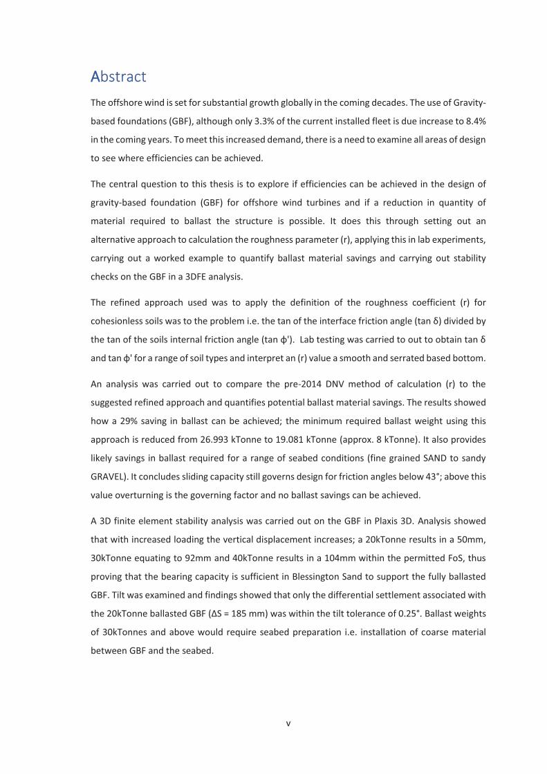
AAbstract The offshore wind is set for substantial growth globally in the coming decades. The use of Gravity-

based foundations (GBF), although only 3.3% of the current installed fleet is due increase to 8.4%

in the coming years. To meet this increased demand, there is a need to examine all areas of design

to see where efficiencies can be achieved.

The central question to this thesis is to explore if efficiencies can be achieved in the design of

gravity-based foundation (GBF) for offshore wind turbines and if a reduction in quantity of

material required to ballast the structure is possible. It does this through setting out an

alternative approach to calculation the roughness parameter (r), applying this in lab experiments,

carrying out a worked example to quantify ballast material savings and carrying out stability

checks on the GBF in a 3DFE analysis.

The refined approach used was to apply the definition of the roughness coefficient (r) for

cohesionless soils was to the problem i.e. the tan of the interface friction angle (tan δ) divided by

the tan of the soils internal friction angle (tan φ'). Lab testing was carried to out to obtain tan δ

and tan φ' for a range of soil types and interpret an (r) value a smooth and serrated based bottom.

An analysis was carried out to compare the pre-2014 DNV method of calculation (r) to the

suggested refined approach and quantifies potential ballast material savings. The results showed

how a 29% saving in ballast can be achieved; the minimum required ballast weight using this

approach is reduced from 26.993 kTonne to 19.081 kTonne (approx. 8 kTonne). It also provides

likely savings in ballast required for a range of seabed conditions (fine grained SAND to sandy

GRAVEL). It concludes sliding capacity still governs design for friction angles below 43°; above this

value overturning is the governing factor and no ballast savings can be achieved.

A 3D finite element stability analysis was carried out on the GBF in Plaxis 3D. Analysis showed

that with increased loading the vertical displacement increases; a 20kTonne results in a 50mm,

30kTonne equating to 92mm and 40kTonne results in a 104mm within the permitted FoS, thus

proving that the bearing capacity is sufficient in Blessington Sand to support the fully ballasted

GBF. Tilt was examined and findings showed that only the differential settlement associated with

the 20kTonne ballasted GBF (ΔS = 185 mm) was within the tilt tolerance of 0.25°. Ballast weights

of 30kTonnes and above would require seabed preparation i.e. installation of coarse material

between GBF and the seabed.

vi

The main contributions this thesis offers offshore designers are steps to applying an alternative

approach to estimating sliding resistance, and quantifies the amount of ballast that can be saved

by using this approach.

vii

DDeclaration Aside from carrying out the testing of the commissioned laboratory work in Section 4, I hereby

declare that this is entirely my own work and that it has not been submitted as an exercise for

the award of a degree ar any other university. I agree to deposit this thesis in the University’s

open access institutional repository or allow the library to do so on my behalf, subject to Irish

Copyright Legislation and Trinity College Library conditions of use and acknowledgement

viii

NNomenclature Abbreviations

API American Petroleum Institute

BS British Standard

CIRIA Construction Industry Research and Information Association

DNV- GL Det Norske Veritas-Germanischer Lloyd

EC Eurocodes

FEA Finite Element Analysis

FEM Finite Element Method

FoS Factor of Safety

FoS Utilisation FoS/minimum FoS required

GBF Gravity Based Foundation

GDG Gavin and Doherty Geosolutions Ltd

HLV Heavy Lifting Vessels

HS Hardening Soil (HS) model

HSSmall Hardening Soil model with small strain stiffness

ISO International Organization for Standards

O&G Oil and Gas

PSD Particle Size Distribution

RNA Rotor Nacelle Assembly

SEAI Sustainable Energy Authority of Ireland

SLS Serviceability limit state

SF Safety Analysis

UDL Uniformly Distributed Load

ULS Ultimate Limit State

ix

Latin Symbols

Effective area

B Width of the footing

c Design cohesion or design undrained shear strength (kN/m2)

c’ Effective cohesion of the soil

, , Correction factors depending on the depth of the foundation

D50 Mean particle size

Relative Density

Young’s Modulus

Triaxial loading stiffness

Odeometer loading stiffness

Triaxial unloaded stiffness

Horizontal loading (Plaxis)

Vertical loading (Plaxis)

G Gravity

Strain shear modulus

Horizontal loading

Horizontal resultant force at the base.

, , : Correction factors depending on the shape of the footing

Resistant moment

m Rate of stress dependency

Moment (Plaxis)

, , Bearing capacity factors (depending on the friction angle)

q Overburden pressure at the level of the foundation-soil interface (kN/m2)

x

Design bearing capacity (kN/m2)

Roughness parameter/coefficient

Ra Ratio of surface roughness

Strength reduction factor in Plaxis

Rk Characteristic resistance

Sk Characteristic load/moment

, , Correction factors depending on the shape of the footing

U Total displacement (Plaxis)

Lateral displacement (Plaxis)

Vertical displacement (Plaxis)

Poisson’s ratio

Vertical load acting during the relevant loading condition

Greek Symbols

Unit weight of soil (kN/m3)

Effective submerged unit weight

Strain level where shear modulus is reduced to about 70% of small-strain shear

modulus

ΔS Differential settlement (mm)

Internal friction angle of soil

Effective internal friction angle of soil

Interface friction angle (between the foundation soil and the structure)

Constant volume friction angle

∑Msf Global factor of safety in Plaxis

Peak friction angle

xi

AAcknowledgements This thesis was initially conceptualised by my employer, Gavin & Doherty Geosolutions Ltd. and

is based on a project I worked on for the SEAI. Thanks to Prof. David Igoe who acted as my

supervisor for this project and offered invaluable advice and insight all through the research. I

would like to thank the Head of Offshore in GDG, Dr. Soroosh Jalilvand for his support. I would

sincerely like to thank my Fiancée, Michelle, for her patience and for looking after our boys, Jonah

and Julien while I worked in this thesis.

1

1 Introduction

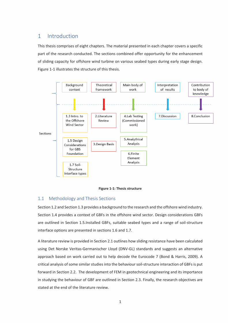
This thesis comprises of eight chapters. The material presented in each chapter covers a specific

part of the research conducted. The sections combined offer opportunity for the enhancement

of sliding capacity for offshore wind turbine on various seabed types during early stage design.

Figure 1-1 illustrates the structure of this thesis.

Figure 1-1: Thesis structure

1.1 Methodology and Thesis Sections

Section 1.2 and Section 1.3 provides a background to the research and the offshore wind industry.

Section 1.4 provides a context of GBFs in the offshore wind sector. Design considerations GBFs

are outlined in Section 1.5.Installed GBFs, suitable seabed types and a range of soil-structure

interface options are presented in sections 1.6 and 1.7.

A literature review is provided in Section 2.1 outlines how sliding resistance have been calculated

using Det Norske Veritas-Germanischer Lloyd (DNV-GL) standards and suggests an alternative

approach based on work carried out to help decode the Eurocode 7 (Bond & Harris, 2009). A

critical analysis of some similar studies into the behaviour soil-structure interaction of GBFs is put

forward in Section 2.2. The development of FEM in geotechnical engineering and its importance

in studying the behaviour of GBF are outlined in Section 2.3. Finally, the research objectives are

stated at the end of the literature review.

2

Section 3 sets out the design basis of this thesis and all relevant calculations, formulae and

assumptions for the calculations and inputs to the finite element analysis (FEA) components of

this MAI project. The geometry of the GBF, water depth and hydrodynamic loads were adopted

from ARUP’s GBF (Smith, et al., 2015) and the turbine interface loads were selected based on

reference loads for a 10MW DTU offshore wind turbine (Velarde, 2016).

The laboratory testing phase (Section 4) of this industry-based MAI project was commissioned by

Gavin and Doherty Geosolutions Ltd (GDG) as part of work carried out on behalf of the

Sustainable Energy Authority of Ireland (SEAI), the testing took place in Trinity College Dublin

(TCD). The addition of Blessington sand as a soil grading was carried out at the request of the

author of this thesis. A series of interface shear tests were undertaken to demonstrate improved

sliding resistance for a range of soil gradings and structural interfaces i) smooth pre-cast concrete,

and ii) a ridged concrete interface. Data from there tests were interpreted and a range of values

for the interface friction angle, sliding ratio and roughness parameter (r) were derived and used

in the ballast requirements (Section 5) and FEA (Section 6).

Section 5 demonstrates saving (in the form of a reduction in the quantity of ballast material

required) that can be achieved from the adoption of the refined approach (improvement on the

DNV pre 2014 method) for calculation of sliding resistance, bearing capacity and overturning

through a preliminary design example for a gravity base foundation supporting an offshore wind

turbine in 45 m water depth through a series of hand calculations.

The Finite Element Analysis (FEA) software Plaxis 3D is employed in Section 6 to analyse the

behaviour of the GBF outlined in Section 3.2 when a series of potential ballast loads are applied.

The FEA quantified vertical and lateral displacements for a serrated base within a factor of safety.

The differential settlement is also calculated.

A discussion on the meaning on the results is presented in 7. The significance of the findings is

highlighted and its applicability to industry is underlined. Some limitations of the thesis are

mentioned and the potential for further study suggested.

Throughout the thesis numerous values and calculation are used. The source, formulae and

calculations are presented the literature review and design basis and then applied in the main

body of the thesis i.e. Sections 4, 5 and 6. Table 3-10 outlines the relationship of values and

calculations used.

3

1.2 Background to the Research

Key factors in the design of GBF are the estimation of sliding capacity, bearing capacity and

overturning. The sliding capacity in conventional concrete GBF concepts is provided by interface

friction at the base of the foundation, as well as, secondary mechanisms such as particle interlock

and passive resistance due to shallow penetration of the foundation in the seabed. In areas with

coarse seabed or shallow bedrock, where limited penetration is available and skirts are not

feasible, the sliding capacity of conventional concrete GBF is mainly governed by the interface

friction at the base. Current design guidelines provide recommendations for assessing the friction

resistance as a function of the dead weight of the structure. However, these approaches are

limited in range of interface geometries considered and tend to underestimate the friction. These

standards also provide limited insight into the sliding resistance for uneven seabed with coarse

surface material such as gravel, boulders and cobbles.

Despite the limited commercial application within the offshore renewable industry to date, GBFs

have advantages over steel piled foundations with respect to;

� Fatigue life;

� Environmental impact through installation noise;

� The need for less specialist fabrication facilities

� Straightforward deployment strategy that is well suited to the narrow weather windows

associated with offshore construction, and in specific.

Presently there are certain combinations of ground conditions and structure type where the use

of a GBF is often considered not feasible as the size of the structure required to resist the lateral

and moment loading is too large. Examples of such situations include;

� Areas with shallow bedrock underlying sandy seabed, which may limit the possibility of

adoption of skirts to the required embedment depth;

� Areas with coarse seabed where there is a mix of gravel, boulders and or a hard and

uneven surface, where seabed preparations required to achieve a flat seabed would be

too costly.

The traditional estimation of this friction resistance in areas with coarse seabed materials is

directly proportional to the dead weight of the substructure. Therefore, to increase the sliding

capacity of the substructure, it is necessary to increase its dead weight using additional ballast or

material weight. This can be very costly due to requirement for procurement, staging and

4

installation of additional ballast, as well as potential increase in the overall size of the structure

that will subsequently increase the requirements for installation vessels. Additionally, the larger

structure will attract higher hydrodynamic loading, which in turn, will increase the demand for

additional ballast or larger footprint of the structure.

To address this issue, and aid in the further development of GBF for marine renewables, this MAI

project aims to further the knowledge of design by refining the design approach and prove that

a reduction in the quantity of ballast material required can be achieved.

1.3 Introduction to Sub-Structures in the Offshore Wind Sector

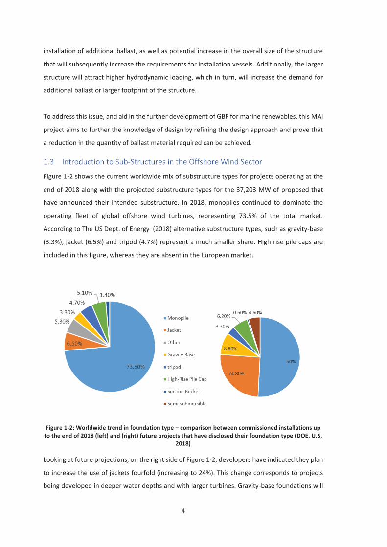
Figure 1-2 shows the current worldwide mix of substructure types for projects operating at the

end of 2018 along with the projected substructure types for the 37,203 MW of proposed that

have announced their intended substructure. In 2018, monopiles continued to dominate the

operating fleet of global offshore wind turbines, representing 73.5% of the total market.

According to The US Dept. of Energy (2018) alternative substructure types, such as gravity-base

(3.3%), jacket (6.5%) and tripod (4.7%) represent a much smaller share. High rise pile caps are

included in this figure, whereas they are absent in the European market.

Figure 1-2: Worldwide trend in foundation type – comparison between commissioned installations up to the end of 2018 (left) and (right) future projects that have disclosed their foundation type (DOE, U.S,

2018)

Looking at future projections, on the right side of Figure 1-2, developers have indicated they plan

to increase the use of jackets fourfold (increasing to 24%). This change corresponds to projects

being developed in deeper water depths and with larger turbines. Gravity-base foundations will

5

also slowly increase their market penetration (increasing to 8.8%). This is anticipated to be

because they do not require pile driving during installation, hence eliminating underwater noise

and associated negative impacts to marine mammals. Floating foundations are required for

projects in water deeper than 60 m and will become more common, projected to increase to 4.6%

of total (DOE, U.S, 2018) in the coming decade.

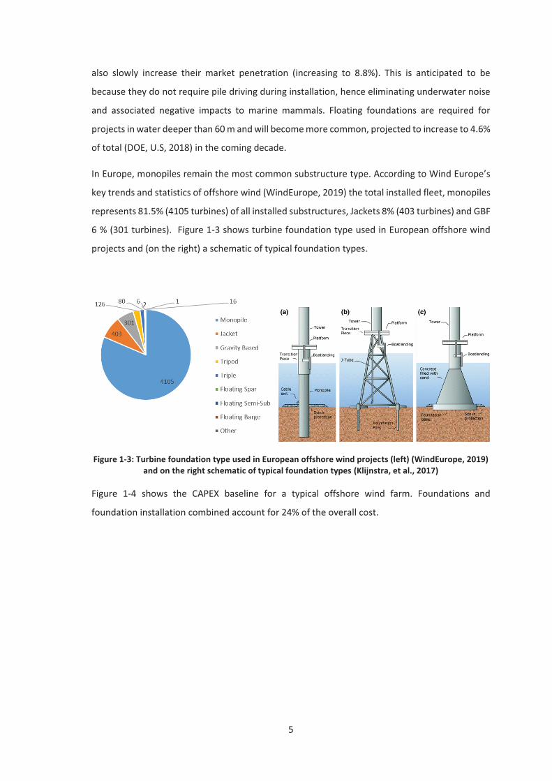
In Europe, monopiles remain the most common substructure type. According to Wind Europe’s

key trends and statistics of offshore wind (WindEurope, 2019) the total installed fleet, monopiles

represents 81.5% (4105 turbines) of all installed substructures, Jackets 8% (403 turbines) and GBF

6 % (301 turbines). Figure 1-3 shows turbine foundation type used in European offshore wind

projects and (on the right) a schematic of typical foundation types.

Figure 1-3: Turbine foundation type used in European offshore wind projects (left) (WindEurope, 2019) and on the right schematic of typical foundation types (Klijnstra, et al., 2017)

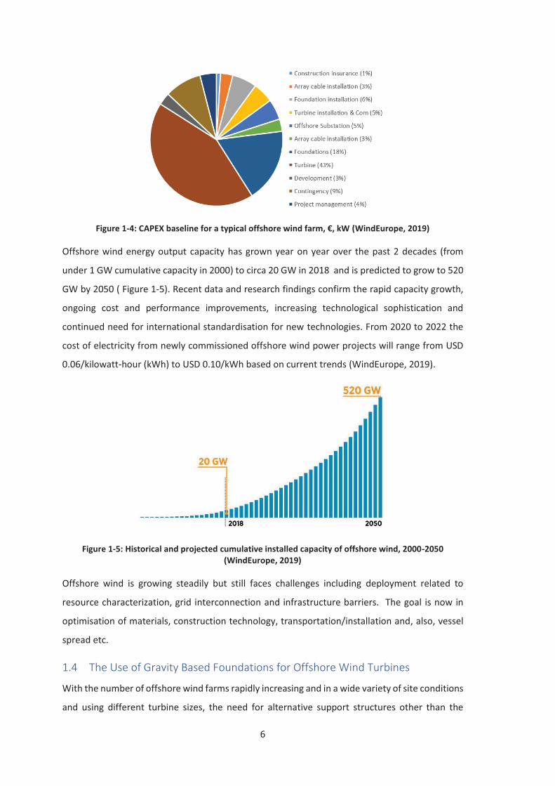
Figure 1-4 shows the CAPEX baseline for a typical offshore wind farm. Foundations and

foundation installation combined account for 24% of the overall cost.

6

Figure 1-4: CAPEX baseline for a typical offshore wind farm, €, kW (WindEurope, 2019)

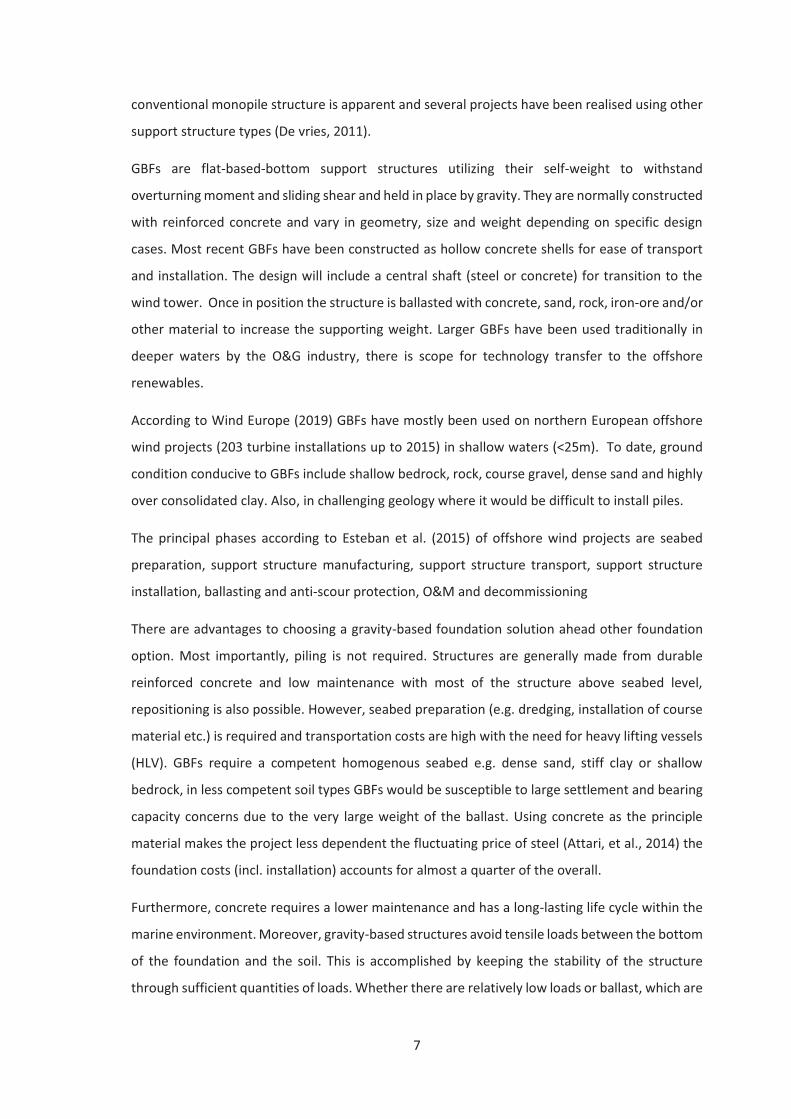
Offshore wind energy output capacity has grown year on year over the past 2 decades (from

under 1 GW cumulative capacity in 2000) to circa 20 GW in 2018 and is predicted to grow to 520

GW by 2050 ( Figure 1-5). Recent data and research findings confirm the rapid capacity growth,

ongoing cost and performance improvements, increasing technological sophistication and

continued need for international standardisation for new technologies. From 2020 to 2022 the

cost of electricity from newly commissioned offshore wind power projects will range from USD

0.06/kilowatt-hour (kWh) to USD 0.10/kWh based on current trends (WindEurope, 2019).

Figure 1-5: Historical and projected cumulative installed capacity of offshore wind, 2000-2050 (WindEurope, 2019)

Offshore wind is growing steadily but still faces challenges including deployment related to

resource characterization, grid interconnection and infrastructure barriers. The goal is now in

optimisation of materials, construction technology, transportation/installation and, also, vessel

spread etc.

1.4 The Use of Gravity Based Foundations for Offshore Wind Turbines

With the number of offshore wind farms rapidly increasing and in a wide variety of site conditions

and using different turbine sizes, the need for alternative support structures other than the

7

conventional monopile structure is apparent and several projects have been realised using other

support structure types (De vries, 2011).

GBFs are flat-based-bottom support structures utilizing their self-weight to withstand

overturning moment and sliding shear and held in place by gravity. They are normally constructed

with reinforced concrete and vary in geometry, size and weight depending on specific design

cases. Most recent GBFs have been constructed as hollow concrete shells for ease of transport

and installation. The design will include a central shaft (steel or concrete) for transition to the

wind tower. Once in position the structure is ballasted with concrete, sand, rock, iron-ore and/or

other material to increase the supporting weight. Larger GBFs have been used traditionally in

deeper waters by the O&G industry, there is scope for technology transfer to the offshore

renewables.

According to Wind Europe (2019) GBFs have mostly been used on northern European offshore

wind projects (203 turbine installations up to 2015) in shallow waters (<25m). To date, ground

condition conducive to GBFs include shallow bedrock, rock, course gravel, dense sand and highly

over consolidated clay. Also, in challenging geology where it would be difficult to install piles.

The principal phases according to Esteban et al. (2015) of offshore wind projects are seabed

preparation, support structure manufacturing, support structure transport, support structure

installation, ballasting and anti-scour protection, O&M and decommissioning

There are advantages to choosing a gravity-based foundation solution ahead other foundation

option. Most importantly, piling is not required. Structures are generally made from durable

reinforced concrete and low maintenance with most of the structure above seabed level,

repositioning is also possible. However, seabed preparation (e.g. dredging, installation of course

material etc.) is required and transportation costs are high with the need for heavy lifting vessels

(HLV). GBFs require a competent homogenous seabed e.g. dense sand, stiff clay or shallow

bedrock, in less competent soil types GBFs would be susceptible to large settlement and bearing

capacity concerns due to the very large weight of the ballast. Using concrete as the principle

material makes the project less dependent the fluctuating price of steel (Attari, et al., 2014) the

foundation costs (incl. installation) accounts for almost a quarter of the overall.

Furthermore, concrete requires a lower maintenance and has a long-lasting life cycle within the

marine environment. Moreover, gravity-based structures avoid tensile loads between the bottom

of the foundation and the soil. This is accomplished by keeping the stability of the structure

through sufficient quantities of loads. Whether there are relatively low loads or ballast, which are

8

easily and cost efficiently provided, GBFs are considered a highly competitive foundation

(4COffshore, 2018).

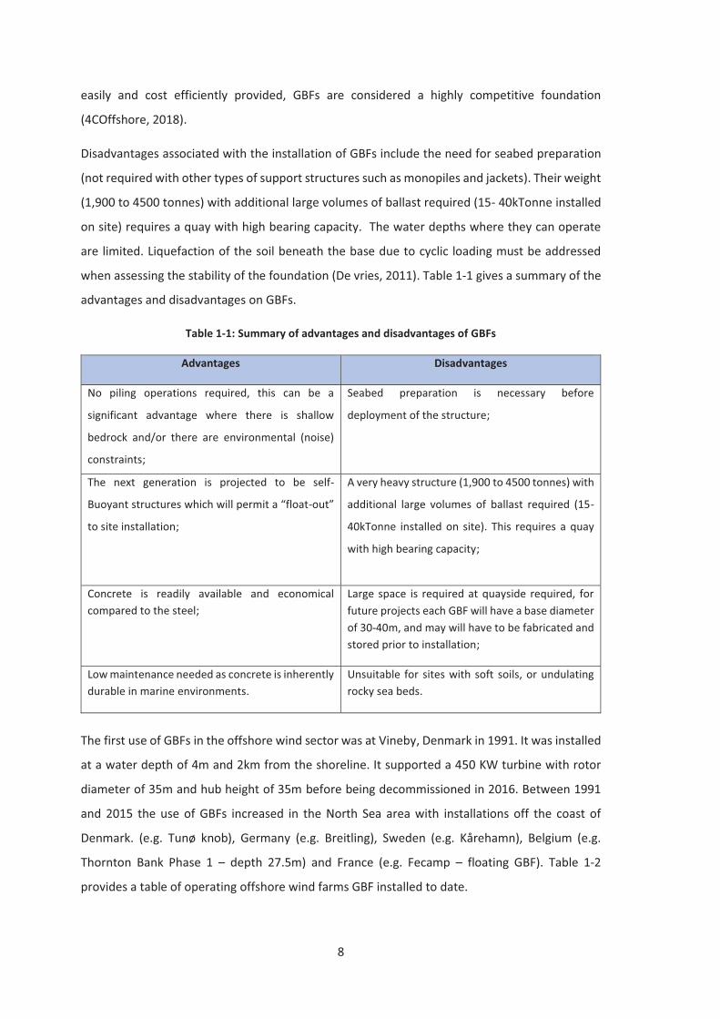
Disadvantages associated with the installation of GBFs include the need for seabed preparation

(not required with other types of support structures such as monopiles and jackets). Their weight

(1,900 to 4500 tonnes) with additional large volumes of ballast required (15- 40kTonne installed

on site) requires a quay with high bearing capacity. The water depths where they can operate

are limited. Liquefaction of the soil beneath the base due to cyclic loading must be addressed

when assessing the stability of the foundation (De vries, 2011). Table 1-1 gives a summary of the

advantages and disadvantages on GBFs.

Table 1-1: Summary of advantages and disadvantages of GBFs

Advantages Disadvantages

No piling operations required, this can be a

significant advantage where there is shallow

bedrock and/or there are environmental (noise)

constraints;

Seabed preparation is necessary before

deployment of the structure;

The next generation is projected to be self-

Buoyant structures which will permit a “float-out”

to site installation;

A very heavy structure (1,900 to 4500 tonnes) with

additional large volumes of ballast required (15-

40kTonne installed on site). This requires a quay

with high bearing capacity;

Concrete is readily available and economical compared to the steel;

Large space is required at quayside required, for future projects each GBF will have a base diameter of 30-40m, and may will have to be fabricated and stored prior to installation;

Low maintenance needed as concrete is inherently durable in marine environments.

Unsuitable for sites with soft soils, or undulating rocky sea beds.

The first use of GBFs in the offshore wind sector was at Vineby, Denmark in 1991. It was installed

at a water depth of 4m and 2km from the shoreline. It supported a 450 KW turbine with rotor

diameter of 35m and hub height of 35m before being decommissioned in 2016. Between 1991

and 2015 the use of GBFs increased in the North Sea area with installations off the coast of

Denmark. (e.g. Tunø knob), Germany (e.g. Breitling), Sweden (e.g. Kårehamn), Belgium (e.g.

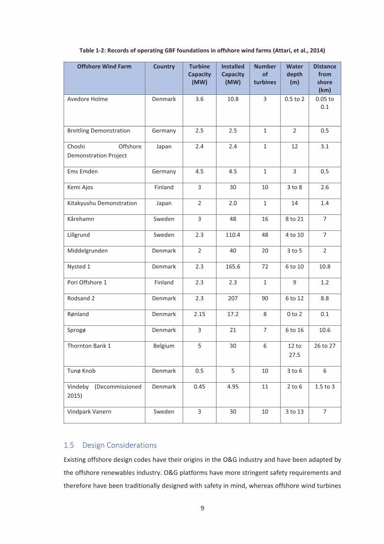
Thornton Bank Phase 1 – depth 27.5m) and France (e.g. Fecamp – floating GBF). Table 1-2

provides a table of operating offshore wind farms GBF installed to date.

9

Table 1-2: Records of operating GBF foundations in offshore wind farms (Attari, et al., 2014)

Offshore Wind Farm

Country

Turbine Capacity

(MW)

Installed Capacity

(MW)

Number of

turbines

Water depth

(m)

Distance from shore (km)

Avedore Holme

Denmark

3.6

10.8

3

0.5 to 2

0.05 to 0.1

Breitling Demonstration Germany 2.5 2.5 1 2 0.5

Choshi Offshore Demonstration Project

Japan 2.4 2.4 1 12 3.1

Ems Emden Germany 4.5 4.5 1 3 0.5

Kemi Ajos Finland 3 30 10 3 to 8 2.6

Kitakyushu Demonstration Japan 2 2.0 1 14 1.4

Kårehamn Sweden 3 48 16 8 to 21 7

Lillgrund Sweden 2.3 110.4 48 4 to 10 7

Middelgrunden Denmark 2 40 20 3 to 5 2

Nysted 1 Denmark 2.3 165.6 72 6 to 10 10.8

Pori Offshore 1 Finland 2.3 2.3 1 9 1.2

Rodsand 2 Denmark 2.3 207 90 6 to 12 8.8

Rønland Denmark 2.15 17.2 8 0 to 2 0.1

Sprogø Denmark 3 21 7 6 to 16 10.6

Thornton Bank 1 Belgium 5 30 6 12 to 27.5

26 to 27

Tunø Knob Denmark 0.5 5 10 3 to 6 6

Vindeby (Decommissioned 2015)

Denmark 0.45 4.95 11 2 to 6 1.5 to 3

Vindpark Vanern Sweden 3 30 10 3 to 13 7

1.5 Design Considerations

Existing offshore design codes have their origins in the O&G industry and have been adapted by

the offshore renewables industry. O&G platforms have more stringent safety requirements and

therefore have been traditionally designed with safety in mind, whereas offshore wind turbines

10

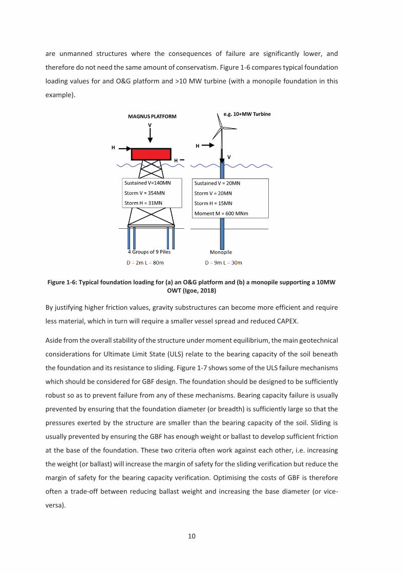
are unmanned structures where the consequences of failure are significantly lower, and

therefore do not need the same amount of conservatism. Figure 1-6 compares typical foundation

loading values for and O&G platform and >10 MW turbine (with a monopile foundation in this

example).

Figure 1-6: Typical foundation loading for (a) an O&G platform and (b) a monopile supporting a 10MW OWT (Igoe, 2018)

By justifying higher friction values, gravity substructures can become more efficient and require

less material, which in turn will require a smaller vessel spread and reduced CAPEX.

Aside from the overall stability of the structure under moment equilibrium, the main geotechnical

considerations for Ultimate Limit State (ULS) relate to the bearing capacity of the soil beneath

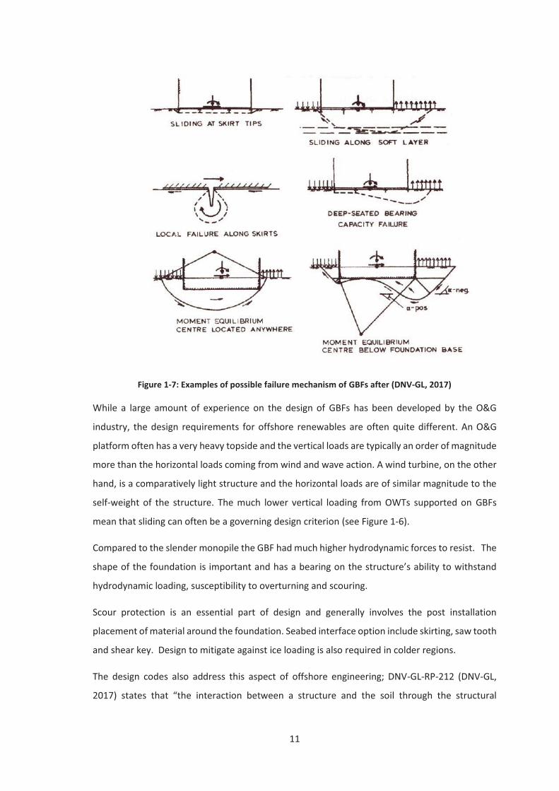
the foundation and its resistance to sliding. Figure 1-7 shows some of the ULS failure mechanisms

which should be considered for GBF design. The foundation should be designed to be sufficiently

robust so as to prevent failure from any of these mechanisms. Bearing capacity failure is usually

prevented by ensuring that the foundation diameter (or breadth) is sufficiently large so that the

pressures exerted by the structure are smaller than the bearing capacity of the soil. Sliding is

usually prevented by ensuring the GBF has enough weight or ballast to develop sufficient friction

at the base of the foundation. These two criteria often work against each other, i.e. increasing

the weight (or ballast) will increase the margin of safety for the sliding verification but reduce the

margin of safety for the bearing capacity verification. Optimising the costs of GBF is therefore

often a trade-off between reducing ballast weight and increasing the base diameter (or vice-

versa).

11

Figure 1-7: Examples of possible failure mechanism of GBFs after (DNV-GL, 2017)

While a large amount of experience on the design of GBFs has been developed by the O&G

industry, the design requirements for offshore renewables are often quite different. An O&G

platform often has a very heavy topside and the vertical loads are typically an order of magnitude

more than the horizontal loads coming from wind and wave action. A wind turbine, on the other

hand, is a comparatively light structure and the horizontal loads are of similar magnitude to the

self-weight of the structure. The much lower vertical loading from OWTs supported on GBFs

mean that sliding can often be a governing design criterion (see Figure 1-6).

Compared to the slender monopile the GBF had much higher hydrodynamic forces to resist. The

shape of the foundation is important and has a bearing on the structure’s ability to withstand

hydrodynamic loading, susceptibility to overturning and scouring.

Scour protection is an essential part of design and generally involves the post installation

placement of material around the foundation. Seabed interface option include skirting, saw tooth

and shear key. Design to mitigate against ice loading is also required in colder regions.

The design codes also address this aspect of offshore engineering; DNV-GL-RP-212 (DNV-GL,

2017) states that “the interaction between a structure and the soil through the structural

12

foundation elements, such as the baseplate and skirt of a GBFs has an influence on several aspects

of structural response namely:

- Global response of dynamically sensitive structures where the foundation stiffness may strongly influence the response;

- Contact stresses between soil and structural elements, governed by soil stiffness and strength and by structural stiffness;

- Settlements of a GBFs; - Stresses in and displacement of piles and structural elements of a jacket platform,

governed by the soil strength and by the stiffness of the piles and structure (DNV-GL, 2017).

1.6 Installed Gravity Based Foundations – Design and Seabed Characteristics

In challenging geology where it would be difficult to install piled GBFs have also been considered.

All Danish projects (see Table 1-2) were installed in shallow rock and clay, Lillgrund and Kårehamn

in are also in shallow rock and clay while, Thornton Bank, Phase 1 in medium grain dense sand.

Geotechnical and geophysical investigations identify potential areas and generally material with

low bearing capacity are dredged e.g. loose sands, muds, clays and silt; thickness of the layers to

be removed can be as deep as 10m (de Temiño, 2013). Installed GBFs have been used where

seabed conditions were coarse to medium dense sand with a gravelly horizon at the bottom and

predominantly chalk.

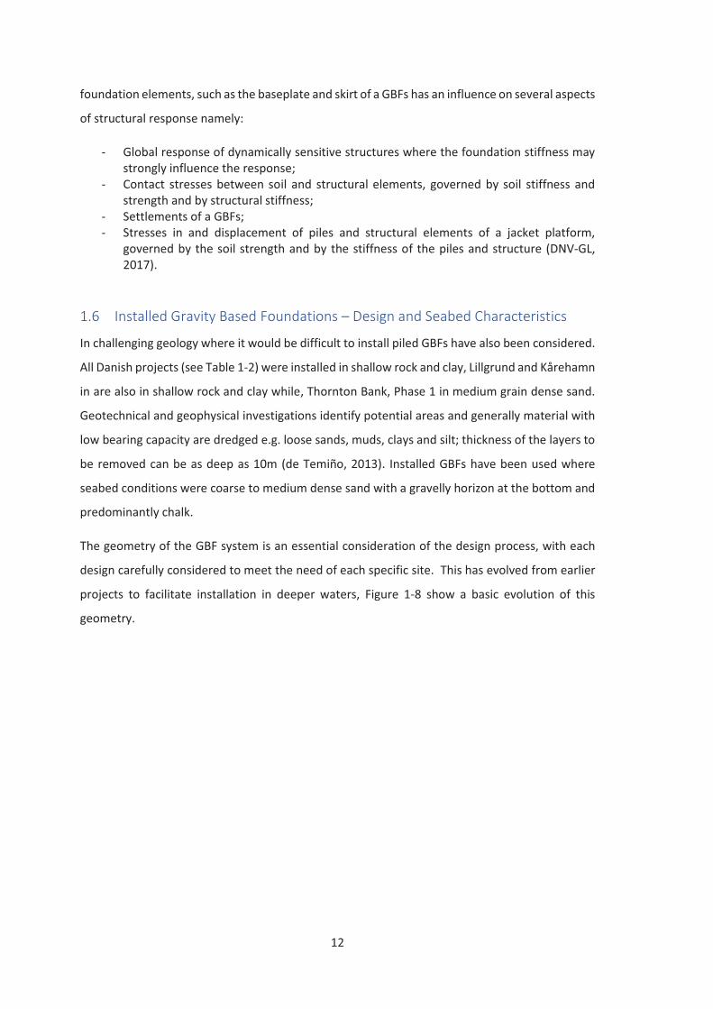
The geometry of the GBF system is an essential consideration of the design process, with each

design carefully considered to meet the need of each specific site. This has evolved from earlier

projects to facilitate installation in deeper waters, Figure 1-8 show a basic evolution of this

geometry.

13

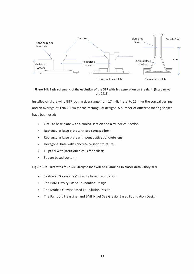
Figure 1-8: Basic schematic of the evolution of the GBF with 3rd generation on the right (Esteban, et al., 2015)

Installed offshore wind GBF footing sizes range from 17m diameter to 25m for the conical designs

and an average of 17m x 17m for the rectangular designs. A number of different footing shapes

have been used:

� Circular base plate with a conical section and a cylindrical section;

� Rectangular base plate with pre-stressed box;

� Rectangular base plate with penetrative concrete legs;

� Hexagonal base with concrete caisson structure;

� Elliptical with partitioned cells for ballast;

� Square based bottom.

Figure 1-9 illustrates four GBF designs that will be examined in closer detail, they are:

� Seatower “Crane-Free” Gravity Based Foundation

� The BAM Gravity Based Foundation Design

� The Strabag Gravity Based Foundation Design

� The Ramboll, Freyssinet and BMT Nigel Gee Gravity Based Foundation Design

14

Figure 1-9: Image of other GBFs considered. Top left: Crane-Free Gravity Base (Seatower, 2013), top right: BAM Van Oord, bottom left: Strabag & Bottom Right: Ramboll, Freyssinet/BMT Nigel Gee (The

Carbon Trust, 2015)

1.6.1 Seatower “Crane-Free” Gravity Based Foundation

The first Seatower Cranefree gravity foundation for offshore wind has been successfully installed

in the British Channel approximately 15 km off the French coast at the Fécamp offshore site at 30

meters water depth. The “crane-free” gravity base concept is a concrete structure with a

relatively thin slab, an intermediate-length conical part, and a cylindrical shaft in the upper part.

This concept was designed, with a hollow interior to be transported by floating out to site with

the support of tugboats, this avoids the use of an expensive and weather-sensitive cranes

(Seatower, 2013).

1.6.2 The BAM Gravity Based Foundation Design

This GBF is made up of more than 1,800 of concrete and weighs over 15,000 tonnes when fully

installed on the seabed with a total height of around 60 metres from the base to the access

platform (BAM, 2017). It is conical shaped structure with a circular base diameter of 40m.

1.6.3 The Strabag Gravity Based Foundation Design

Both of the Strabag’s GBF designs have a geometrical slab and a cylinder in the upper part and

use the pre-stressed concrete technique, they are suitable for water depths up to approximately

45 m. The concepts employ a joint transportation and installation of the foundation and the wind

15

turbine generator which reduces the number of operations carried out at sea during the

installation phase allow the structure to be completely disassembled. A purposed vessel is used,

called STRABAG Carrier is used to transport and installation. A lifted design using a floated crane.

Pre-stressed concrete is used and small skirts may be required depending on soil conditions.

Integrated footing plates are used for load transfer from concrete to soil and to avoid gaps

between concrete and soil and developing of scour (The Carbon Trust, 2015).

1.6.4 The Ramboll, Freyssinet and BMT Nigel Gee Gravity Based Foundation Design

This design uses an integrated approach to onshore construction, transportation and offshore

installation. It employs a specialised semi-submersible transportation and Installation barge

where the turbine and tower can be pre-installed onshore if required (The Carbon Trust, 2015).

1.7 A review of Soil-Structural Interface Types

Some installations are designed to require no penetration while others require a penetration to

withstand horizontal loading and shear forces. The sliding resistance will always increase where

there is significant seabed-structure penetration. This section reviews the following interface

options:

� Skirting

� Concrete Grouted Interface

� Flat based bottom

� Serrated based bottoms

1.7.1 Skirting

In O&G installations seabed penetration can be achieved through the use of a “skirt” at the base

of the GBF. however, no evidence was found that skirting has been used on the installations of

offshore wind farms. Skirting has been employed to increase the sliding resistance, transfer loads

to where the soil is stronger, provide a closed compartment to facilitate grouting under base and

provide scour protection. The foundation penetrates into the seabed, increasing the bearing area.

The load is transferred down to the underlying layers, lateral load capacity is improved by the

skirt’s lateral resistance and the moment load capacity raised, and the foundation resists uplift

better (Ahmadi & Ghazavi, 2012).

Skirting runs along the edge (and sometimes additional skirts internally) penetrating into the

ground below the seabed. The penetration depth of the skirts can range from 0.5m to 30 m,

depending on the softness of the underlying soil and size of the upper structure (Gourvenec &

Barnett, 2011). The skirts form an enclosed space where the soil is confined and works as a unit

16

with the overlain foundation to transfer superstructure load to soil essentially at the level of skirt

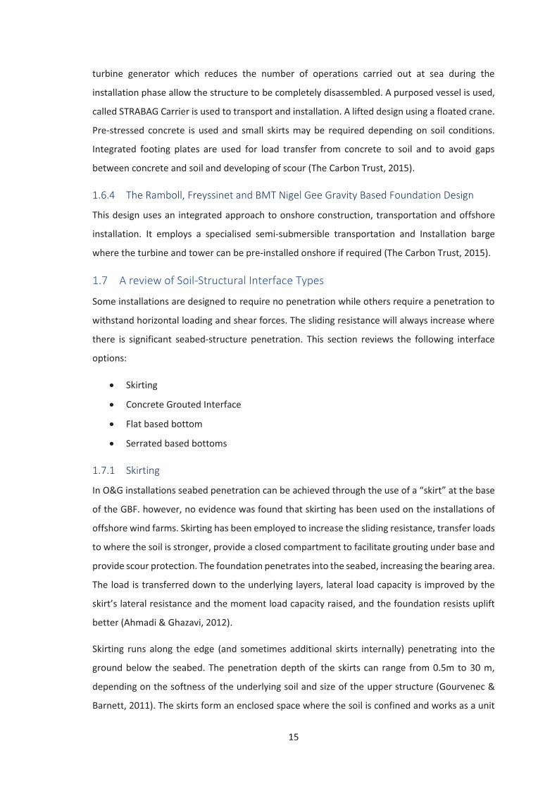
tip. Reinforced concrete skirts have also been used on concrete structures. Figure 1-10 illustrates

a skirt on the flanks of a GBF.

Figure 1-10: Image of a skirt on the flanks of a GBFs (Seatower, 2013)

1.7.2 Concrete Grouted Interface

Grout is used to assist with securing structures to the seabed. The use of grout in O&G GBFs is

commonplace and has been used to carry out the following function:

� avoid further penetration and to keep the platform vertical;

� ensure uniform stresses against the foundation slab and avoid unintended overstressing

of structural elements during continued ballasting and environmental loading;

� prevent piping from water pockets below the base during environmental loading (Tistel,

et al., 2015)

In the offshore sector wind grout can be used similarly. It has been applied at Seatower’s Crane-

free demonstrator project where grout was pumped in between the seabed and the soffit GBF to

fill the void and to provide fill contact (de Temiño, 2013).

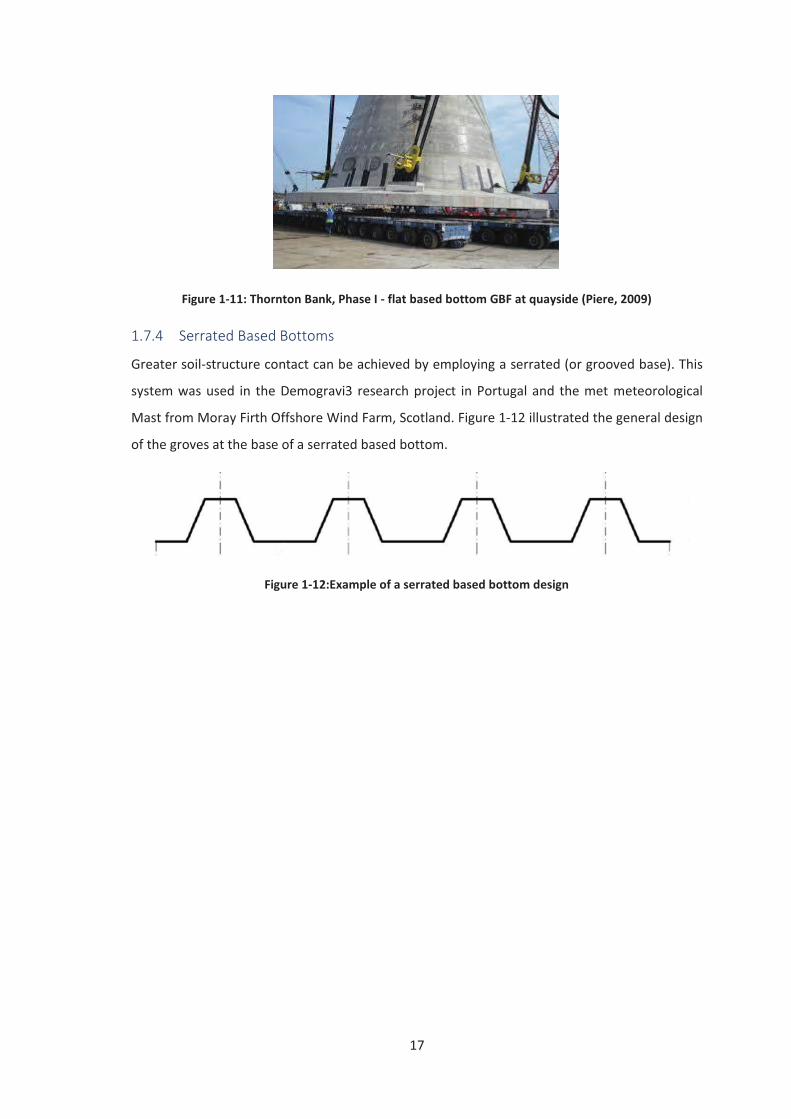
1.7.3 Flat Based Bottom

Some GBF installations proceed without any penetration into the sea bed e.g. where a flat bases

bottom is used. This seems to have been the case in offshore wind to date. This is backed up by

Temiño’s master’s thesis (2013) statement that “skirting has not yet been introduced into

offshore wind it was assumed that all of the installations to date are flat based bottomed”. Figure

1-11 shows an example of a flat-based-bottom GBF.

17

Figure 1-11: Thornton Bank, Phase I - flat based bottom GBF at quayside (Piere, 2009)

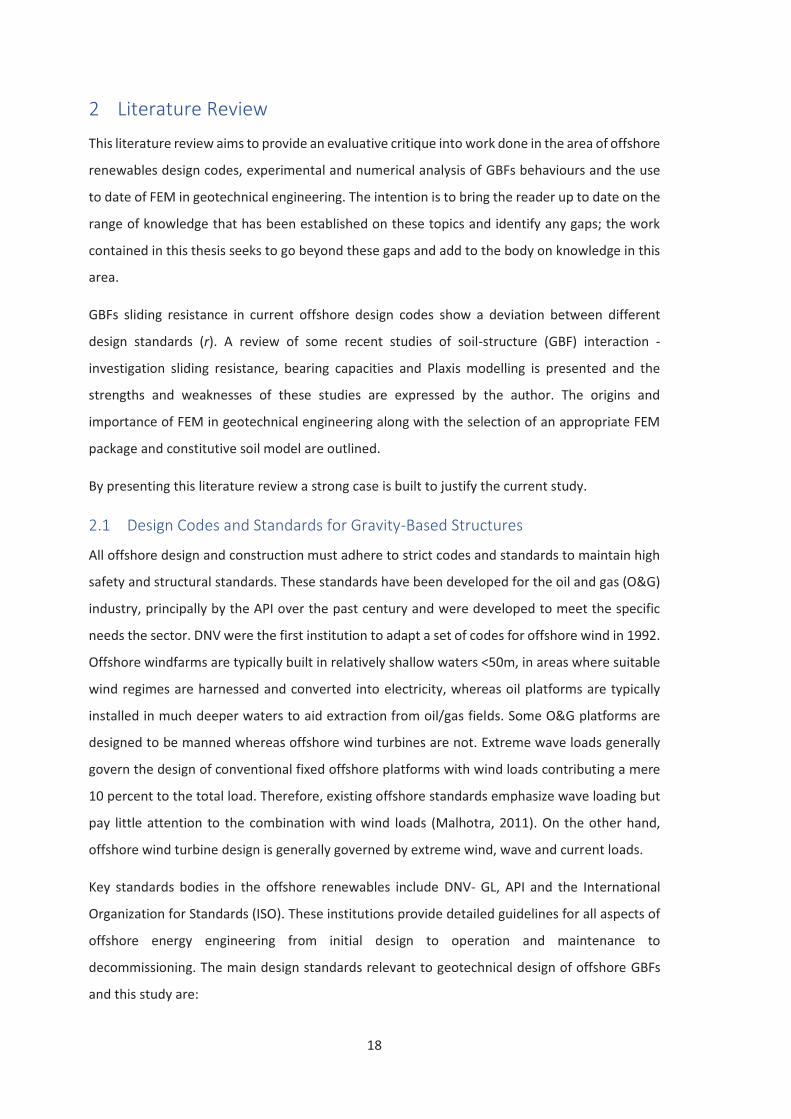
1.7.4 Serrated Based Bottoms

Greater soil-structure contact can be achieved by employing a serrated (or grooved base). This

system was used in the Demogravi3 research project in Portugal and the met meteorological

Mast from Moray Firth Offshore Wind Farm, Scotland. Figure 1-12 illustrated the general design

of the groves at the base of a serrated based bottom.

Figure 1-12:Example of a serrated based bottom design

18

2 Literature Review

This literature review aims to provide an evaluative critique into work done in the area of offshore

renewables design codes, experimental and numerical analysis of GBFs behaviours and the use

to date of FEM in geotechnical engineering. The intention is to bring the reader up to date on the

range of knowledge that has been established on these topics and identify any gaps; the work

contained in this thesis seeks to go beyond these gaps and add to the body on knowledge in this

area.

GBFs sliding resistance in current offshore design codes show a deviation between different

design standards (r). A review of some recent studies of soil-structure (GBF) interaction -

investigation sliding resistance, bearing capacities and Plaxis modelling is presented and the

strengths and weaknesses of these studies are expressed by the author. The origins and

importance of FEM in geotechnical engineering along with the selection of an appropriate FEM

package and constitutive soil model are outlined.

By presenting this literature review a strong case is built to justify the current study.

2.1 Design Codes and Standards for Gravity-Based Structures

All offshore design and construction must adhere to strict codes and standards to maintain high

safety and structural standards. These standards have been developed for the oil and gas (O&G)

industry, principally by the API over the past century and were developed to meet the specific

needs the sector. DNV were the first institution to adapt a set of codes for offshore wind in 1992.

Offshore windfarms are typically built in relatively shallow waters <50m, in areas where suitable

wind regimes are harnessed and converted into electricity, whereas oil platforms are typically

installed in much deeper waters to aid extraction from oil/gas fields. Some O&G platforms are

designed to be manned whereas offshore wind turbines are not. Extreme wave loads generally

govern the design of conventional fixed offshore platforms with wind loads contributing a mere

10 percent to the total load. Therefore, existing offshore standards emphasize wave loading but

pay little attention to the combination with wind loads (Malhotra, 2011). On the other hand,

offshore wind turbine design is generally governed by extreme wind, wave and current loads.

Key standards bodies in the offshore renewables include DNV- GL, API and the International

Organization for Standards (ISO). These institutions provide detailed guidelines for all aspects of

offshore energy engineering from initial design to operation and maintenance to

decommissioning. The main design standards relevant to geotechnical design of offshore GBFs

and this study are:

19

� DNV-OS-J101 (2013) – Design of Offshore Wind Turbine Structures (superseded) (DNV-

GL, 2013)

� DNVGL-ST-0126 (2018) – Support structures for wind turbines (current) (DNV-GL, 2018)

� DNVGL-RP-C212 (2017) – Offshore soil mechanics and geotechnical engineering (current)

(DNV-GL, 2017)

� ISO-19901-4 (2014) – Petroleum and natural gas industries – Specific requirements for

offshore structures – Part 4: Geotechnical and foundation design considerations (current)

(ISO, 2014)

� API-RP-2GEO (2011) – Geotechnical and foundation design considerations (current) (API,

2011)

The treatment of the bearing capacity of GBF systems is broadly similar across all these standards,

having been developed originally by the O&G industry (API standards). The treatment of sliding

resistance for GBFs deviates somewhat between different design standards. The API-RP-2GEO

(API, 2011) standards propose the maximum horizontal load for the extreme condition of pure

sliding should be limited to:

Equation

2-1

Where is the maximum total horizontal load applied to the base of the foundation at failure

under drained conditions, is the actual vertical load acting during the relevant loading

condition, is the soils internal friction angle. The guidelines suggest that this equation assumes

that the full soil resistance in mobilised along the interface between the foundation and the soil

(i.e. full soil-soil contact is assumed) which should be assessed on a case by case basis. It is also

suggested that it may be more appropriate to consider the use of different interface friction

angles, , between the foundation soil and the structure. The equation would therefore become:

Equation

2-2

The DNV approach for sliding varies from the API approach somewhat. Prior to 2014 DNV

guidelines (DNV-GL, 2013) suggests that “foundations subject to horizontal loading must be

investigated for sufficient sliding resistance”. Such foundations must meet the following criterion:

20

Equation

2-3

Where is the effective area of the foundation and c’ is the effective cohesion of the soil.

These guidelines also state that the ratio of horizontal friction to vertical load must be limited to

0.4, such that:

Equation

2-4

Hence, for a cohesionless soil the equation simplifies to: ϕ

Equation

2-5

More recent updates to the DNV design standards (DNV-GL, 2017), have modified the above

equations by removing the maximum H/V ratio of 0.4 and using a roughness parameter (r). which

is a factor with a value of 1.0 for soil against soil and takes lesser values for soil against structure.

Hence, the updated form of calculating horizontal sliding resistance is:

Equation

2-6

Similar to equation 3, for a cohesionless soil, the above equation simplifies to:

Equation

2-7

No guidance is provided as to the value of r. The roughness parameter (r) can be related to the

interface friction angle through the equation below:

Equation

2-8

21

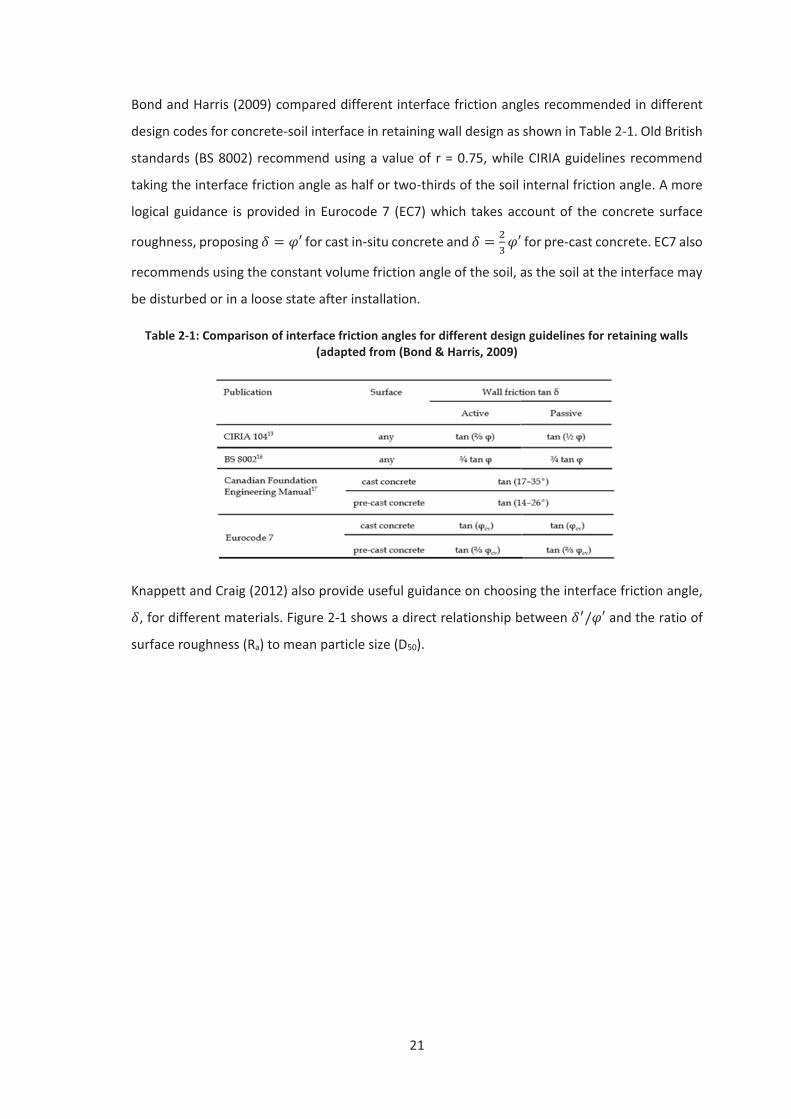
Bond and Harris (2009) compared different interface friction angles recommended in different

design codes for concrete-soil interface in retaining wall design as shown in Table 2-1. Old British

standards (BS 8002) recommend using a value of r = 0.75, while CIRIA guidelines recommend

taking the interface friction angle as half or two-thirds of the soil internal friction angle. A more

logical guidance is provided in Eurocode 7 (EC7) which takes account of the concrete surface

roughness, proposing for cast in-situ concrete and for pre-cast concrete. EC7 also

recommends using the constant volume friction angle of the soil, as the soil at the interface may

be disturbed or in a loose state after installation.

Table 2-1: Comparison of interface friction angles for different design guidelines for retaining walls (adapted from (Bond & Harris, 2009)

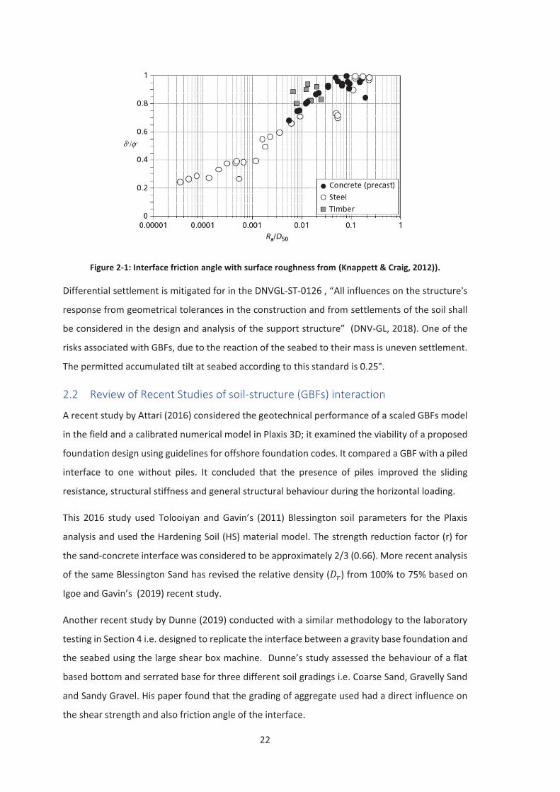
Knappett and Craig (2012) also provide useful guidance on choosing the interface friction angle,

, for different materials. Figure 2-1 shows a direct relationship between and the ratio of

surface roughness (Ra) to mean particle size (D50).

22

Figure 2-1: Interface friction angle with surface roughness from (Knappett & Craig, 2012)).

Differential settlement is mitigated for in the DNVGL-ST-0126 , “All influences on the structure's

response from geometrical tolerances in the construction and from settlements of the soil shall

be considered in the design and analysis of the support structure” (DNV-GL, 2018). One of the

risks associated with GBFs, due to the reaction of the seabed to their mass is uneven settlement.

The permitted accumulated tilt at seabed according to this standard is 0.25°.

2.2 Review of Recent Studies of soil-structure (GBFs) interaction

A recent study by Attari (2016) considered the geotechnical performance of a scaled GBFs model

in the field and a calibrated numerical model in Plaxis 3D; it examined the viability of a proposed

foundation design using guidelines for offshore foundation codes. It compared a GBF with a piled

interface to one without piles. It concluded that the presence of piles improved the sliding

resistance, structural stiffness and general structural behaviour during the horizontal loading.

This 2016 study used Tolooiyan and Gavin’s (2011) Blessington soil parameters for the Plaxis

analysis and used the Hardening Soil (HS) material model. The strength reduction factor (r) for

the sand-concrete interface was considered to be approximately 2/3 (0.66). More recent analysis

of the same Blessington Sand has revised the relative density ( ) from 100% to 75% based on

Igoe and Gavin’s (2019) recent study.

Another recent study by Dunne (2019) conducted with a similar methodology to the laboratory

testing in Section 4 i.e. designed to replicate the interface between a gravity base foundation and

the seabed using the large shear box machine. Dunne’s study assessed the behaviour of a flat

based bottom and serrated base for three different soil gradings i.e. Coarse Sand, Gravelly Sand

and Sandy Gravel. His paper found that the grading of aggregate used had a direct influence on

the shear strength and also friction angle of the interface.

23

His results suggest that DNV guidelines provide a more optimum design approach based on these

tests, indicating that a serrated interface results in upwards of a 30% improvement on horizontal

sliding friction compared to that of a smooth interface. It was, however, unclear why the serrated

interface over the smooth interface were much less defined for the coarser aggregate grading.

Differential settlement of the GBF will be calculated in Plaxis 3D. Smith et al.’s method (2015) to

calculate differential settlement sought to establish different stages of settlement splitting the

calculation into three key areas; (i) immediate settlements calculated via traditional analytical

methods; (ii) consolidation settlement and rate of consolidation; and (iii) settlement analysis by

means of numerical modelling techniques . Settlement results generated in Plaxis and OASYS

were compared. The Plaxis set up applied a uniform distributed load (UDL) of 200 kN/ over a

base plate with 40m diameter. The sand layers were modelled using the Mohr-Coulomb (MC)

failure criterion assuming drained condition upon loading.

The initial settlement result of 193mm was questioned by the author as eccentricity of the

foundation loading that would result in trapezoidal pressure distribution and with further

refinement a differential settlement (ΔS = 135 mm) was achieved. This produced a foundation tilt

of the of 0.2°, thus satisfying the criteria adopted of 0.25°at design and 0.75° installation

tolerance, giving a total design tolerance of 1°. Smith et al.’s paper (2015) limited itself by using

the more basic Mohr-Coulomb (MC) soil model; a more accurate result is expected in the current

MAI project by using the HSSmall soil model.

2.3 Finite Element Analysis in Geotechnical Engineering

The use of FEM in geotechnical engineering started in the 1960s. Woodward and Clough (1967)

utilised FEM to assess the stress stability and movement in embankments and Reyes and Deane

(1966) applied the approach to analyse underground openings in rocks. Its application spread

rapidly as advancement in computer power and software improved. It has been a reliable tool in

solving geotechnical problems and if employed with proper knowledge and understanding, can

carry out realistic predictions, applicable in practical geotechnical problems (Zdravković & Potts,

1999).

Some literature is available on the topic of modelling of gravity base foundations using FEM,

Potvin (1990), who analysed the horizontal load-bearing resistance of a skirted GBF using the

commercial FEM package Abaqus, also, Murray et al. (1992) and Sturm (2011) carried out

important work.

24

Soil exhibits complicated and nonlinear behaviour, which is influenced by several factors, such

as the origin of soil deposits, the grain size, the surrounding environment, the stress history and

the load condition among others (Attari, 2016).

2.3.1 Selection of FEM Software

There are a number of commercial and open source options FEM software options available to

conduct geotechnical 3DFE analysis e.g. Abaqus, Ansys, PISA, SAFE etc. Some have a good range

of analysis possible (linear, non-linear, static, dynamic, construction stages, etc), comprehensive

in-built element libraries, good error messaging, high quality meshing techniques, powerful

graphical presentation etc. However, there can be issues with relating to having to write scripts

externally, more general purpose rather than geotechnical specific, difficult to learn etc.

Plaxis was chosen because it has been in the market for quite some time and there is more

academic work evaluated by experts available. Also, it is specific to geotechnical problem solving

and has powerful graphical presentation. Although Plaxis does sometime struggle with complex

geometry, the GBF in this thesis is relatively straight forward. Plaxis which was developed by Delft

University by Brinkgrove, Broere and Watermann allows for theoretically solid computational

modelling in a windows-based platform.

2.3.2 Constitutive Soil Model

Numerous constitutive soil models have been developed over the past 40 years for the modelling

of stress-strain behaviour of soils. The capabilities and shortcomings of these models are not

always easy to ascertain and the requirement for determination of parameters not always

uniform. It is consequently difficult to determine which model to select for a particular task (Lade,

2005).

The stress-strain behaviour of soil depends on several factors, namely stress levels, loading

direction, anisotropy, rate of loading, drainage and aging (Elhakim, 2005). Constitutive soil

models describe the complex stress-strain behaviour of soil.

The degree of accuracy required will determine whether a simple linear elastic-plastic or a more

complex method is employed. The simplest available constitutive model is derived from Hooke’s

law of linear elasticity, and only requires two input parameters, the Young’s Modulus (E) and the

Poisson’s ratio (v) (PLAXIS, 2019).

Constitutive soil models within Plaxis 3D include the Linear Elastic model (LE), Mohr-Coulomb

model (MC), Soft Soil model (SS), Hardening Soil model (HS), Soft Soil Creep model (SSC) and

25

Jointed Rock model (JR). In this thesis, the Hardening Soil small (HSsmall) model has been adopted

following the recommendation of Tolooiyan & Gavin (2011)

2.3.2.1 HS Small

The Hardening Soil model with small-strain stiffness (HSsmall) is a modification of the Hardening

soil model that accounts for the increased stiffness of the soils at small strains. At low strain levels

most, soils exhibit a higher stiffness than at engineering strain levels. And this stiffness varies non-

linearly with strain (PLAXIS, 2019).

Two additional material parameters are required and . is the strain shear modulus

and is the strain level at which the shear modulus id reduced to about 70% of the small-strain

shear modulus (PLAXIS, 2019). The HSSmall is the model to be used in section 6 because it gives

a more reliable displacement than HS model in working load conditions. Table 2-2 shows the

required inputs into Plaxis for a HSsmall soil model.

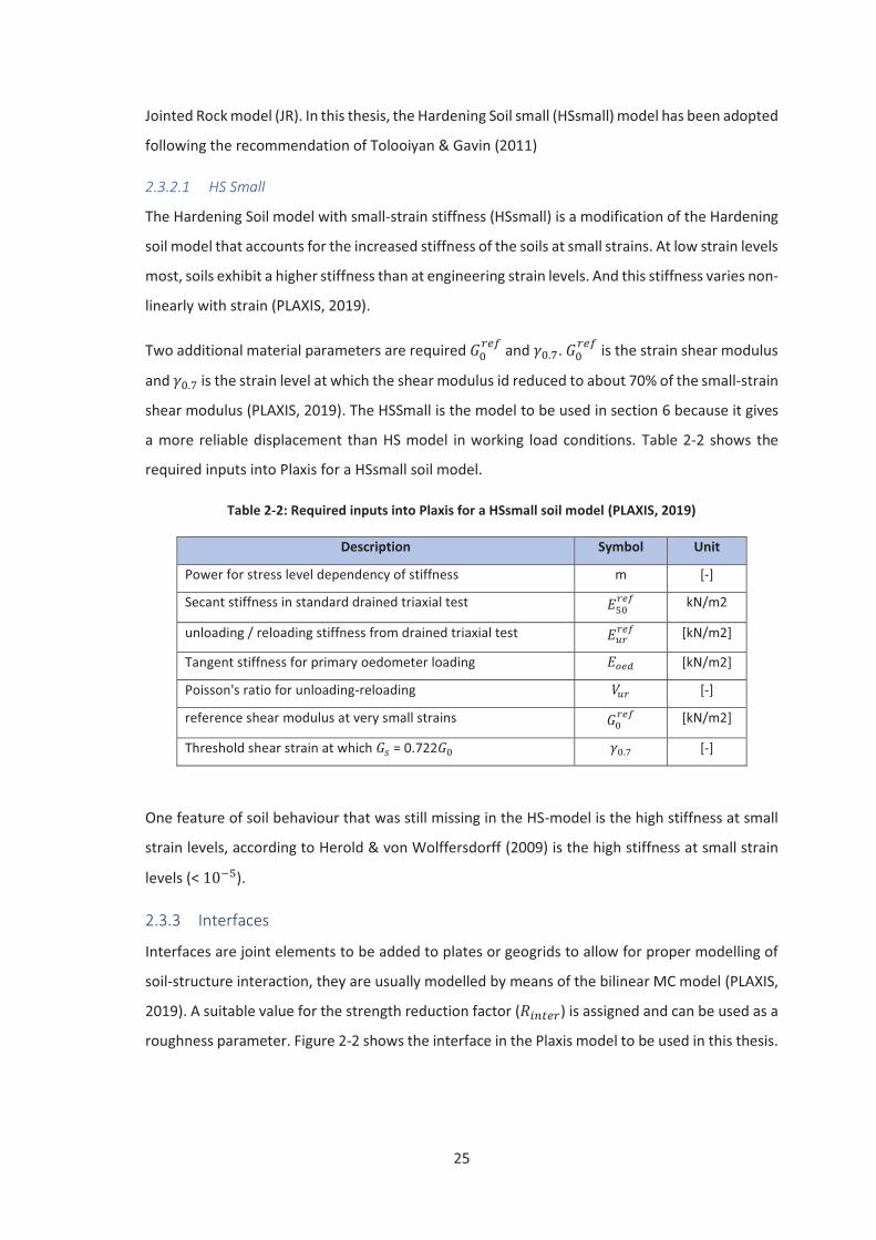
Table 2-2: Required inputs into Plaxis for a HSsmall soil model (PLAXIS, 2019)

Description Symbol Unit

Power for stress level dependency of stiffness m [-]

Secant stiffness in standard drained triaxial test kN/m2

unloading / reloading stiffness from drained triaxial test [kN/m2]

Tangent stiffness for primary oedometer loading [kN/m2]

Poisson's ratio for unloading-reloading [-]

reference shear modulus at very small strains [kN/m2]

Threshold shear strain at which = 0.722 [-]

One feature of soil behaviour that was still missing in the HS-model is the high stiffness at small

strain levels, according to Herold & von Wolffersdorff (2009) is the high stiffness at small strain

levels (< ).

2.3.3 Interfaces

Interfaces are joint elements to be added to plates or geogrids to allow for proper modelling of

soil-structure interaction, they are usually modelled by means of the bilinear MC model (PLAXIS,

2019). A suitable value for the strength reduction factor ( ) is assigned and can be used as a

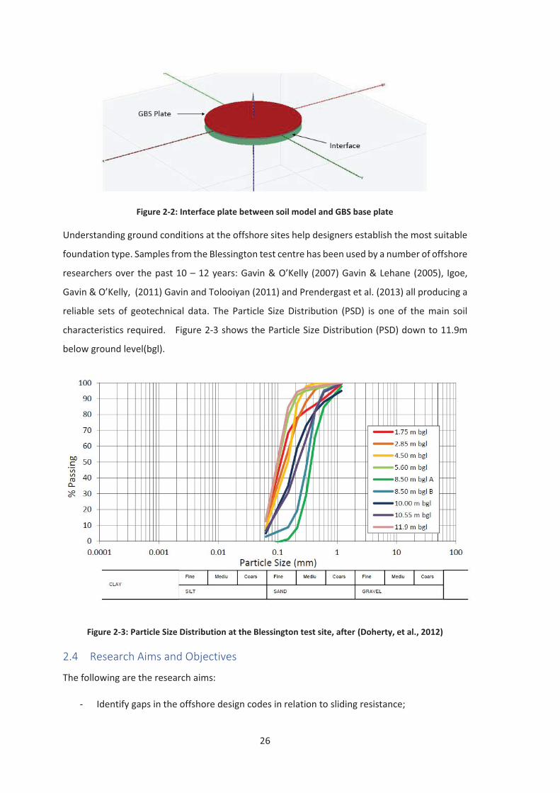
roughness parameter. Figure 2-2 shows the interface in the Plaxis model to be used in this thesis.

26

Figure 2-2: Interface plate between soil model and GBS base plate

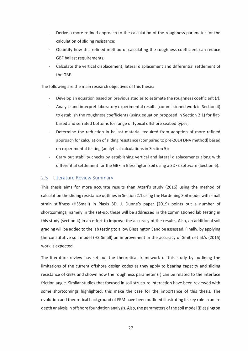
Understanding ground conditions at the offshore sites help designers establish the most suitable

foundation type. Samples from the Blessington test centre has been used by a number of offshore

researchers over the past 10 – 12 years: Gavin & O’Kelly (2007) Gavin & Lehane (2005), Igoe,

Gavin & O’Kelly, (2011) Gavin and Tolooiyan (2011) and Prendergast et al. (2013) all producing a

reliable sets of geotechnical data. The Particle Size Distribution (PSD) is one of the main soil

characteristics required. Figure 2-3 shows the Particle Size Distribution (PSD) down to 11.9m

below ground level(bgl).

Figure 2-3: Particle Size Distribution at the Blessington test site, after (Doherty, et al., 2012)

2.4 Research Aims and Objectives

The following are the research aims:

- Identify gaps in the offshore design codes in relation to sliding resistance;

27

- Derive a more refined approach to the calculation of the roughness parameter for the

calculation of sliding resistance;

- Quantify how this refined method of calculating the roughness coefficient can reduce

GBF ballast requirements;

- Calculate the vertical displacement, lateral displacement and differential settlement of

the GBF.

The following are the main research objectives of this thesis:

- Develop an equation based on previous studies to estimate the roughness coefficient (r).

- Analyse and interpret laboratory experimental results (commissioned work in Section 4)

to establish the roughness coefficients (using equation proposed in Section 2.1) for flat-

based and serrated bottoms for range of typical offshore seabed types;

- Determine the reduction in ballast material required from adoption of more refined

approach for calculation of sliding resistance (compared to pre-2014 DNV method) based

on experimental testing (analytical calculations in Section 5);

- Carry out stability checks by establishing vertical and lateral displacements along with

differential settlement for the GBF in Blessington Soil using a 3DFE software (Section 6).

2.5 Literature Review Summary

This thesis aims for more accurate results than Attari’s study (2016) using the method of

calculation the sliding resistance outlines in Section 2.1 using the Hardening Soil model with small

strain stiffness (HSSmall) in Plaxis 3D. J. Dunne’s paper (2019) points out a number of

shortcomings, namely in the set-up, these will be addressed in the commissioned lab testing in

this study (section 4) in an effort to improve the accuracy of the results. Also, an additional soil

grading will be added to the lab testing to allow Blessington Sand be assessed. Finally, by applying

the constitutive soil model (HS Small) an improvement in the accuracy of Smith et al.’s (2015)

work is expected.

The literature review has set out the theoretical framework of this study by outlining the

limitations of the current offshore design codes as they apply to bearing capacity and sliding

resistance of GBFs and shown how the roughness parameter (r) can be related to the interface

friction angle. Similar studies that focused in soil-structure interaction have been reviewed with

some shortcomings highlighted, this make the case for the importance of this thesis. The

evolution and theoretical background of FEM have been outlined illustrating its key role in an in-

depth analysis in offshore foundation analysis. Also, the parameters of the soil model (Blessington

28

Sand) and constitutive soil model (HS Small) used were defined. Finally, the research aims and

objectives were defined.

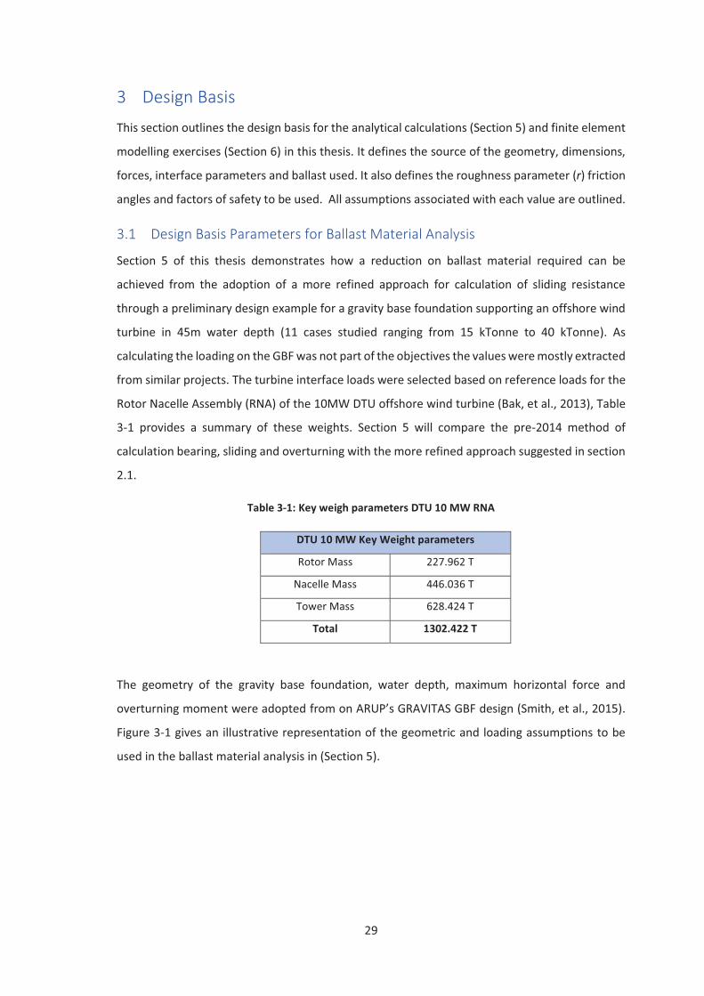
29

3 Design Basis

This section outlines the design basis for the analytical calculations (Section 5) and finite element

modelling exercises (Section 6) in this thesis. It defines the source of the geometry, dimensions,

forces, interface parameters and ballast used. It also defines the roughness parameter (r) friction

angles and factors of safety to be used. All assumptions associated with each value are outlined.

3.1 Design Basis Parameters for Ballast Material Analysis

Section 5 of this thesis demonstrates how a reduction on ballast material required can be

achieved from the adoption of a more refined approach for calculation of sliding resistance

through a preliminary design example for a gravity base foundation supporting an offshore wind

turbine in 45m water depth (11 cases studied ranging from 15 kTonne to 40 kTonne). As

calculating the loading on the GBF was not part of the objectives the values were mostly extracted

from similar projects. The turbine interface loads were selected based on reference loads for the

Rotor Nacelle Assembly (RNA) of the 10MW DTU offshore wind turbine (Bak, et al., 2013), Table

3-1 provides a summary of these weights. Section 5 will compare the pre-2014 method of

calculation bearing, sliding and overturning with the more refined approach suggested in section

2.1.

Table 3-1: Key weigh parameters DTU 10 MW RNA

DTU 10 MW Key Weight parameters

Rotor Mass 227.962 T

Nacelle Mass 446.036 T

Tower Mass 628.424 T

Total 1302.422 T

The geometry of the gravity base foundation, water depth, maximum horizontal force and

overturning moment were adopted from on ARUP’s GRAVITAS GBF design (Smith, et al., 2015).

Figure 3-1 gives an illustrative representation of the geometric and loading assumptions to be

used in the ballast material analysis in (Section 5).

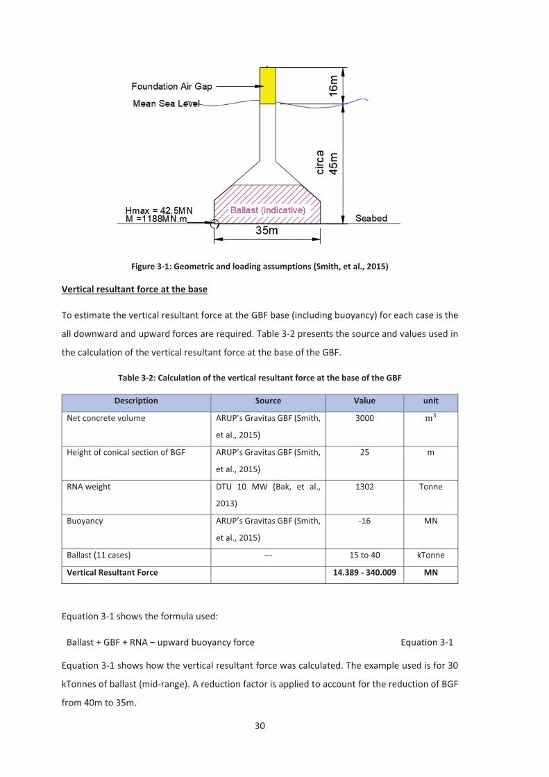
30

Figure 3-1: Geometric and loading assumptions (Smith, et al., 2015)

Vertical resultant force at the base

To estimate the vertical resultant force at the GBF base (including buoyancy) for each case is the

all downward and upward forces are required. Table 3-2 presents the source and values used in

the calculation of the vertical resultant force at the base of the GBF.

Table 3-2: Calculation of the vertical resultant force at the base of the GBF

Description Source Value unit

Net concrete volume ARUP’s Gravitas GBF (Smith,

et al., 2015)

3000

Height of conical section of BGF ARUP’s Gravitas GBF (Smith,

et al., 2015)

25 m

RNA weight DTU 10 MW (Bak, et al.,

2013)

1302 Tonne

Buoyancy ARUP’s Gravitas GBF (Smith,

et al., 2015)

-16 MN

Ballast (11 cases) --- 15 to 40 kTonne

Vertical Resultant Force 14.389 - 340.009 MN

Equation 3-1 shows the formula used:

Ballast + GBF + RNA – upward buoyancy force Equation 3-1

Equation 3-1 shows how the vertical resultant force was calculated. The example used is for 30

kTonnes of ballast (mid-range). A reduction factor is applied to account for the reduction of BGF

from 40m to 35m.

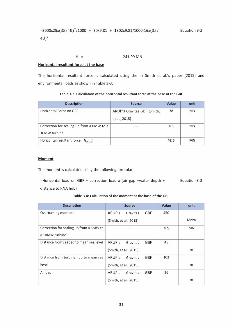
31

=3000x25x /1000 + 30x9.81 + 1302x9.81/1000-16x

Equation 3-2

H = 241.99 MN

Horizontal resultant force at the base

The horizontal resultant force is calculated using the in Smith et al.’s paper (2015) and

environmental loads as shown in Table 3-3.

Table 3-3: Calculation of the horizontal resultant force at the base of the GBF

Description Source Value unit

Horizontal Force on GBF ARUP’s Gravitas GBF (Smith,

et al., 2015)

38 MN

Correction for scaling up from a 6MW to a

10MW turbine

--- 4.5 MN

Horizontal resultant force ( ) 42.5 MN

Moment

The moment is calculated using the following formula:

=Horizontal load on GBF + correction load x (air gap +water depth +

distance to RNA hub)

Equation 3-3

Table 3-4: Calculation of the moment at the base of the GBF

Description Source Value unit

Overturning moment ARUP’s Gravitas GBF

(Smith, et al., 2015)

450

MNm

Correction for scaling up from a 6MW to

a 10MW turbine

--- 4.5 MN

Distance from seabed to mean sea level ARUP’s Gravitas GBF

(Smith, et al., 2015)

45

m

Distance from turbine hub to mean sea

level

ARUP’s Gravitas GBF

(Smith, et al., 2015)

103

m

Air gap ARUP’s Gravitas GBF

(Smith, et al., 2015)

16

m

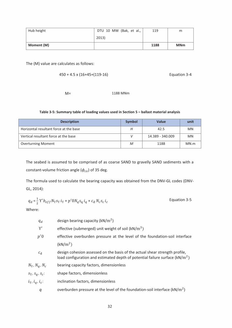
32

Hub height DTU 10 MW (Bak, et al.,

2013)

119 m

Moment (M) 1188 MNm

The (M) value are calculates as follows:

450 + 4.5 x (16+45+(119-16) Equation 3-4

M= 1188 MNm

Table 3-5: Summary table of loading values used in Section 5 – ballast material analysis

Description Symbol Value unit

Horizontal resultant force at the base H 42.5 MN

Vertical resultant force at the base V 14.389 - 340.009 MN

Overturning Moment M 1188 MN.m

The seabed is assumed to be comprised of as coarse SAND to gravelly SAND sediments with a

constant-volume friction angle ( ) of 35 deg.

The formula used to calculate the bearing capacity was obtained from the DNV-GL codes (DNV-

GL, 2014):

= + + Equation 3-5

Where:

design bearing capacity (kN/ )

effective (submerged) unit weight of soil (kN/

effective overburden pressure at the level of the foundation-soil interface

(kN/

design cohesion assessed on the basis of the actual shear strength profile, load configuration and estimated depth of potential failure surface (kN/

, , bearing capacity factors, dimensionless

, , : shape factors, dimensionless

, , : inclination factors, dimensionless

q overburden pressure at the level of the foundation-soil interface (kN/ )

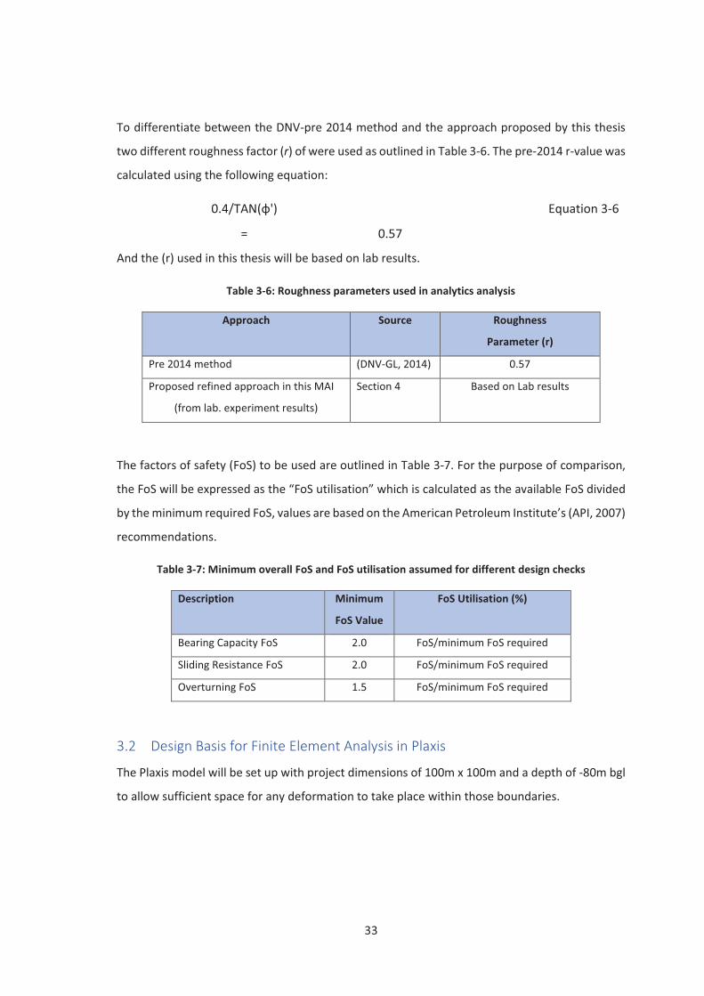
33

To differentiate between the DNV-pre 2014 method and the approach proposed by this thesis

two different roughness factor (r) of were used as outlined in Table 3-6. The pre-2014 r-value was

calculated using the following equation:

0.4/TAN(φ') Equation 3-6

= 0.57

And the (r) used in this thesis will be based on lab results.

Table 3-6: Roughness parameters used in analytics analysis

Approach Source Roughness

Parameter (r)

Pre 2014 method (DNV-GL, 2014) 0.57

Proposed refined approach in this MAI

(from lab. experiment results)

Section 4 Based on Lab results

The factors of safety (FoS) to be used are outlined in Table 3-7. For the purpose of comparison,

the FoS will be expressed as the “FoS utilisation” which is calculated as the available FoS divided

by the minimum required FoS, values are based on the American Petroleum Institute’s (API, 2007)

recommendations.

Table 3-7: Minimum overall FoS and FoS utilisation assumed for different design checks

Description Minimum

FoS Value

FoS Utilisation (%)

Bearing Capacity FoS 2.0 FoS/minimum FoS required

Sliding Resistance FoS 2.0 FoS/minimum FoS required

Overturning FoS 1.5 FoS/minimum FoS required

3.2 Design Basis for Finite Element Analysis in Plaxis

The Plaxis model will be set up with project dimensions of 100m x 100m and a depth of -80m bgl

to allow sufficient space for any deformation to take place within those boundaries.

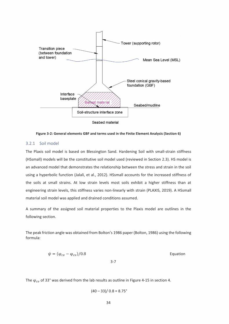
34

Figure 3-2: General elements GBF and terms used in the Finite Element Analysis (Section 6)

3.2.1 Soil model

The Plaxis soil model is based on Blessington Sand. Hardening Soil with small-strain stiffness

(HSsmall) models will be the constitutive soil model used (reviewed in Section 2.3). HS model is

an advanced model that demonstrates the relationship between the stress and strain in the soil

using a hyperbolic function (Jalali, et al., 2012). HSsmall accounts for the increased stiffness of

the soils at small strains. At low strain levels most soils exhibit a higher stiffness than at

engineering strain levels, this stiffness varies non-linearly with strain (PLAXIS, 2019). A HSsmall

material soil model was applied and drained conditions assumed.

A summary of the assigned soil material properties to the Plaxis model are outlines in the

following section.

The peak friction angle was obtained from Bolton’s 1986 paper (Bolton, 1986) using the following formula:

Equation

3-7

The of 33° was derived from the lab results as outline in Figure 4-15 in section 4.

(40 – 33)/ 0.8 = 8.75°

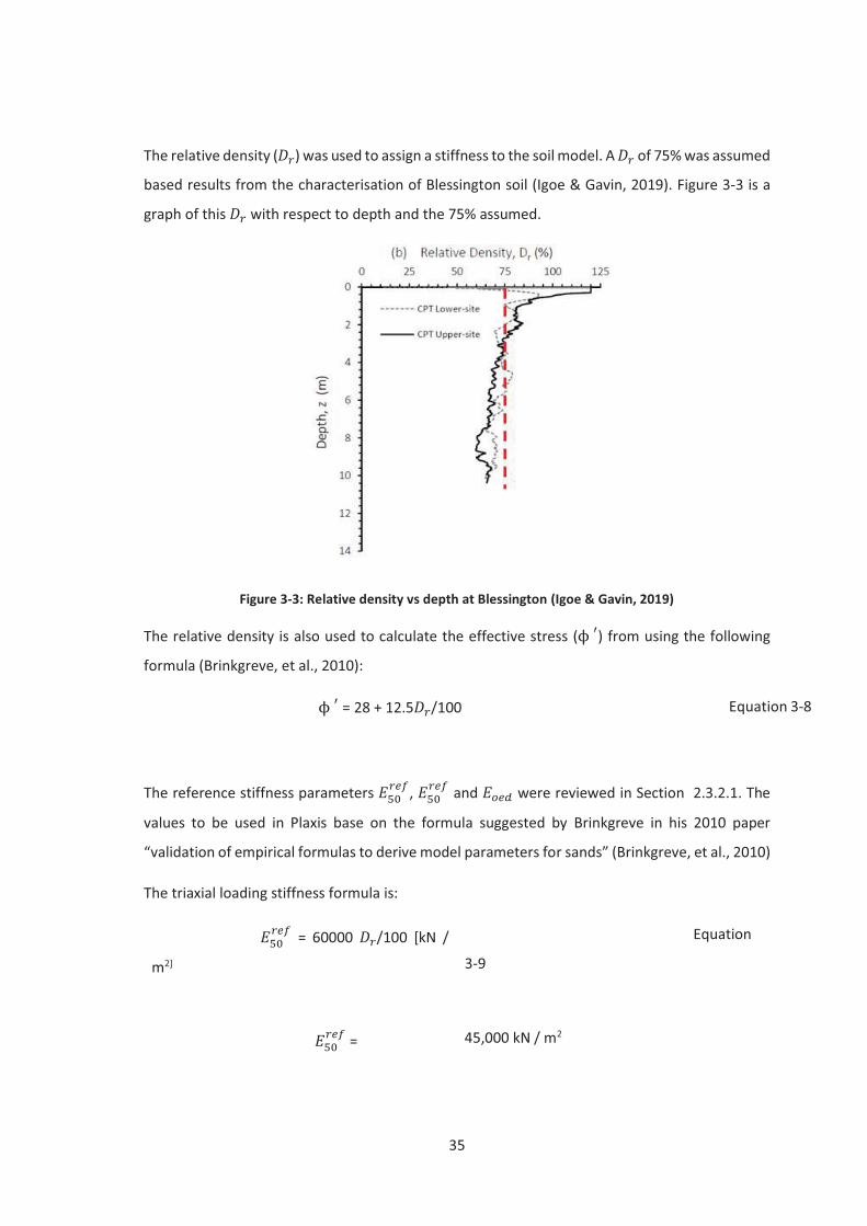
35

The relative density ( ) was used to assign a stiffness to the soil model. A of 75% was assumed

based results from the characterisation of Blessington soil (Igoe & Gavin, 2019). Figure 3-3 is a

graph of this with respect to depth and the 75% assumed.

Figure 3-3: Relative density vs depth at Blessington (Igoe & Gavin, 2019)

The relative density is also used to calculate the effective stress ( ) from using the following

formula (Brinkgreve, et al., 2010):

= 28 + 12.5 /100 Equation 3-8

The reference stiffness parameters , and were reviewed in Section 2.3.2.1. The

values to be used in Plaxis base on the formula suggested by Brinkgreve in his 2010 paper

“validation of empirical formulas to derive model parameters for sands” (Brinkgreve, et al., 2010)

The triaxial loading stiffness formula is:

= 60000 /100 [kN /

m2]

Equation

3-9

= 45,000 kN / m2

36

The oedometer loading stiffness formula is:

= 60000 /100 [kN / m2 Equation 3-

10

= 45,000 kN / m2

The triaxial unloaded stiffness formula in the same publication is:

= 108000 + 68000 /100 [kN /

m2]

Equation 3-

11

However, three times the value equation 3-5 was used.

= 135,000 kN / m2

The actual stiffness is stress-dependent. The rate of stress dependency (m) is observed to be

negatively correlated with the density. The following formula is proposed for m, as suggested by

Brinkgreve (2010):

m = 0.7 - /320 =0.465 Equation 3-12

Brinkgreve et al. suggests a Poisson ratio for unloading and reloading, , of 0.2 (Brinkgreve,

et al., 2010).

and are two additional material parameters required for HSS. is the strain shear

modulus and is the strain level at which the shear modulus is reduced to about 70% of the

small-strain shear modulus (PLAXIS, 2019). These two values were also obtained from Brinkgreve

(Brinkgreve, et al., 2010) using the following formulae:

= 60000 + 68000 /100 Equation 3-

13

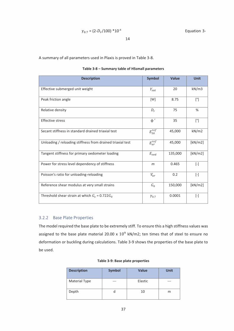
37

= (2- /100) *10-4 Equation 3-

14

A summary of all parameters used in Plaxis is proved in Table 3-8.

Table 3-8 – Summary table of HSsmall parameters

Description Symbol Value Unit

Effective submerged unit weight 20 kN/m3

Peak friction angle [Ψ] 8.75 [°]

Relative density 75 %

Effective stress 35 [°]

Secant stiffness in standard drained triaxial test 45,000 kN/m2

Unloading / reloading stiffness from drained triaxial test 45,000 [kN/m2]

Tangent stiffness for primary oedometer loading 135,000 [kN/m2]

Power for stress level dependency of stiffness m 0.465 [-]

Poisson's ratio for unloading-reloading 0.2 [-]

Reference shear modulus at very small strains 150,000 [kN/m2]

Threshold shear strain at which = 0.722 0.0001 [-]

3.2.2 Base Plate Properties

The model required the base plate to be extremely stiff. To ensure this a high stiffness values was

assigned to the base plate material 20.00 x kN/m2; ten times that of steel to ensure no

deformation or buckling during calculations. Table 3-9 shows the properties of the base plate to

be used.

Table 3-9: Base plate properties

Description Symbol Value Unit

Material Type --- Elastic ---

Depth d 10 m

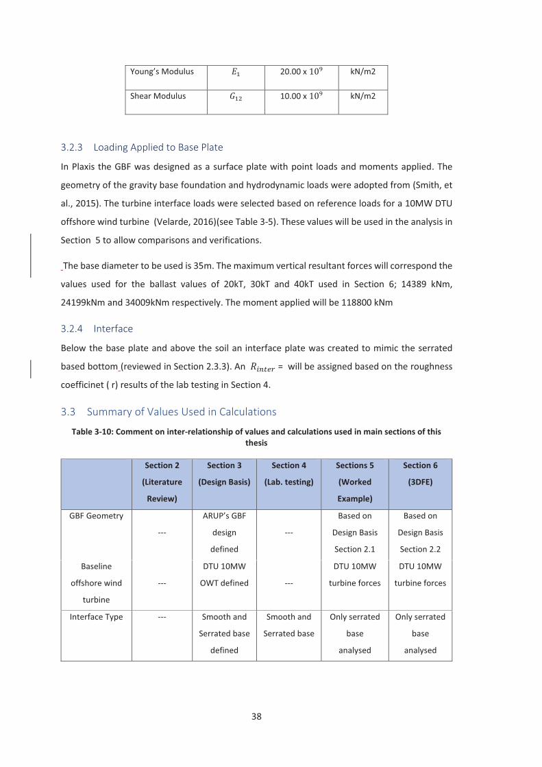
38

Young’s Modulus 20.00 x kN/m2

Shear Modulus 10.00 x kN/m2

3.2.3 Loading Applied to Base Plate

In Plaxis the GBF was designed as a surface plate with point loads and moments applied. The

geometry of the gravity base foundation and hydrodynamic loads were adopted from (Smith, et

al., 2015). The turbine interface loads were selected based on reference loads for a 10MW DTU

offshore wind turbine (Velarde, 2016)(see Table 3-5). These values will be used in the analysis in

Section 5 to allow comparisons and verifications.

The base diameter to be used is 35m. The maximum vertical resultant forces will correspond the

values used for the ballast values of 20kT, 30kT and 40kT used in Section 6; 14389 kNm,

24199kNm and 34009kNm respectively. The moment applied will be 118800 kNm

3.2.4 Interface

Below the base plate and above the soil an interface plate was created to mimic the serrated

based bottom (reviewed in Section 2.3.3). An = will be assigned based on the roughness

coefficinet ( r) results of the lab testing in Section 4.

3.3 Summary of Values Used in Calculations

Table 3-10: Comment on inter-relationship of values and calculations used in main sections of this thesis

Section 2

(Literature

Review)

Section 3

(Design Basis)

Section 4

(Lab. testing)

Sections 5

(Worked

Example)

Section 6

(3DFE)

GBF Geometry

---

ARUP’s GBF

design

defined

---

Based on

Design Basis

Section 2.1

Based on

Design Basis

Section 2.2

Baseline

offshore wind

turbine

---

DTU 10MW

OWT defined

---

DTU 10MW

turbine forces

DTU 10MW

turbine forces

Interface Type --- Smooth and

Serrated base

defined

Smooth and

Serrated base

Only serrated

base

analysed

Only serrated

base

analysed

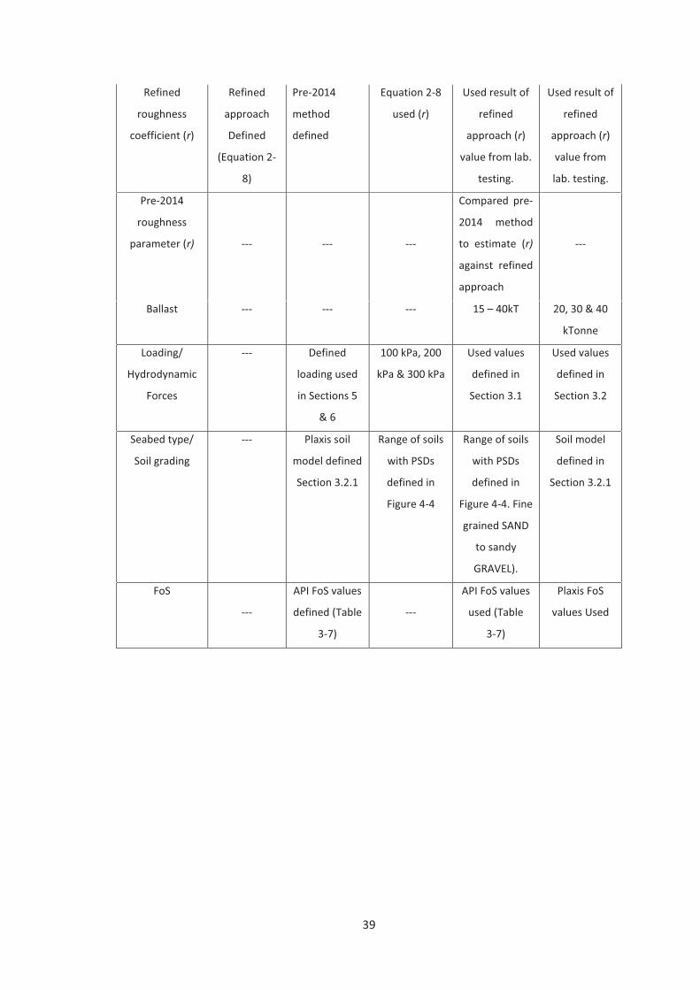
39

Refined

roughness

coefficient (r)

Refined

approach

Defined

(Equation 2-

8)

Pre-2014

method

defined

Equation 2-8

used (r)

Used result of

refined

approach (r)

value from lab.

testing.

Used result of

refined

approach (r)

value from

lab. testing.

Pre-2014

roughness

parameter (r)

---

---

---

Compared pre-

2014 method

to estimate (r)

against refined

approach

---

Ballast --- --- --- 15 – 40kT 20, 30 & 40

kTonne

Loading/

Hydrodynamic

Forces

--- Defined

loading used

in Sections 5

& 6

100 kPa, 200

kPa & 300 kPa

Used values

defined in

Section 3.1

Used values

defined in

Section 3.2

Seabed type/

Soil grading

--- Plaxis soil

model defined

Section 3.2.1

Range of soils

with PSDs

defined in

Figure 4-4

Range of soils

with PSDs

defined in

Figure 4-4. Fine

grained SAND

to sandy

GRAVEL).

Soil model

defined in

Section 3.2.1

FoS

---

API FoS values

defined (Table

3-7)

---

API FoS values

used (Table

3-7)

Plaxis FoS

values Used

40

4 Laboratory Testing and Interpretation

The laboratory testing phase of this industry-based MAI project was commissioned by Gavin and

Doherty Geosolutions Ltd (GDG) as part of work carried out for the SEAI. The design of the

experimental work and, in particular, the addition of Blessington sand as a soil grading was

instigated by the author of this thesis. Experiments were carried out by the lab technician and

supervised by Dr. David Igoe.

Analysing sliding resistance in a series of shear box tests were undertaken using large shear box

apparatus in the Geotechnical Laboratory in the department of Civil, Structural and

Environmental Engineering at Trinity College Dublin.

This section provides the details of methodology including interface geometries considered and

soil gradings used, as well as, the results obtained including variation in sliding resistance with

increasing vertical load and associated interface friction angles.

4.1 Laboratory Testing Objectives

A series of large shear box tests were undertaken in order to provide estimation of interface

friction for different GBF interface types and soil gradings. The objective of the study is to provide

insight into underlying mechanisms/phenomena that contribute to the sliding resistance of

conventional concrete GBF interface and to investigate upper and lower bound interface friction

for a range of soil gradings.

The following laboratory tests were undertaken using a large shear box setup with dimensions

300 x 300mm

� 12 no. tests with soil-soil interface

� 12 no. tests with soil-smooth concrete interface

� 12 no. tests with soil-ridged concrete interface

4.2 Laboratory Testing Methodology

4.2.1 Large Shear box apparatus

The large shear box apparatus, shown in Figure 4-1, tests a sample which measures 300mm x

300mm in plan, with a maximum sample depth of 200mm. The box section of the apparatus is

split in half, with the bottom half allowing horizontal movement, with the top reacting against a

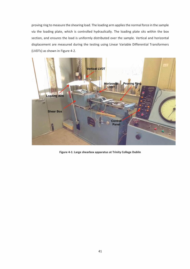
41

proving ring to measure the shearing load. The loading arm applies the normal force in the sample

via the loading plate, which is controlled hydraulically. The loading plate sits within the box

section, and ensures the load is uniformly distributed over the sample. Vertical and horizontal

displacement are measured during the testing using Linear Variable Differential Transformers

(LVDTs) as shown in Figure 4-2.

Figure 4-1: Large shearbox apparatus at Trinity College Dublin

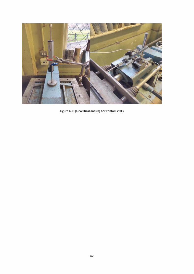
42

Figure 4-2: (a) Vertical and (b) horizontal LVDTs

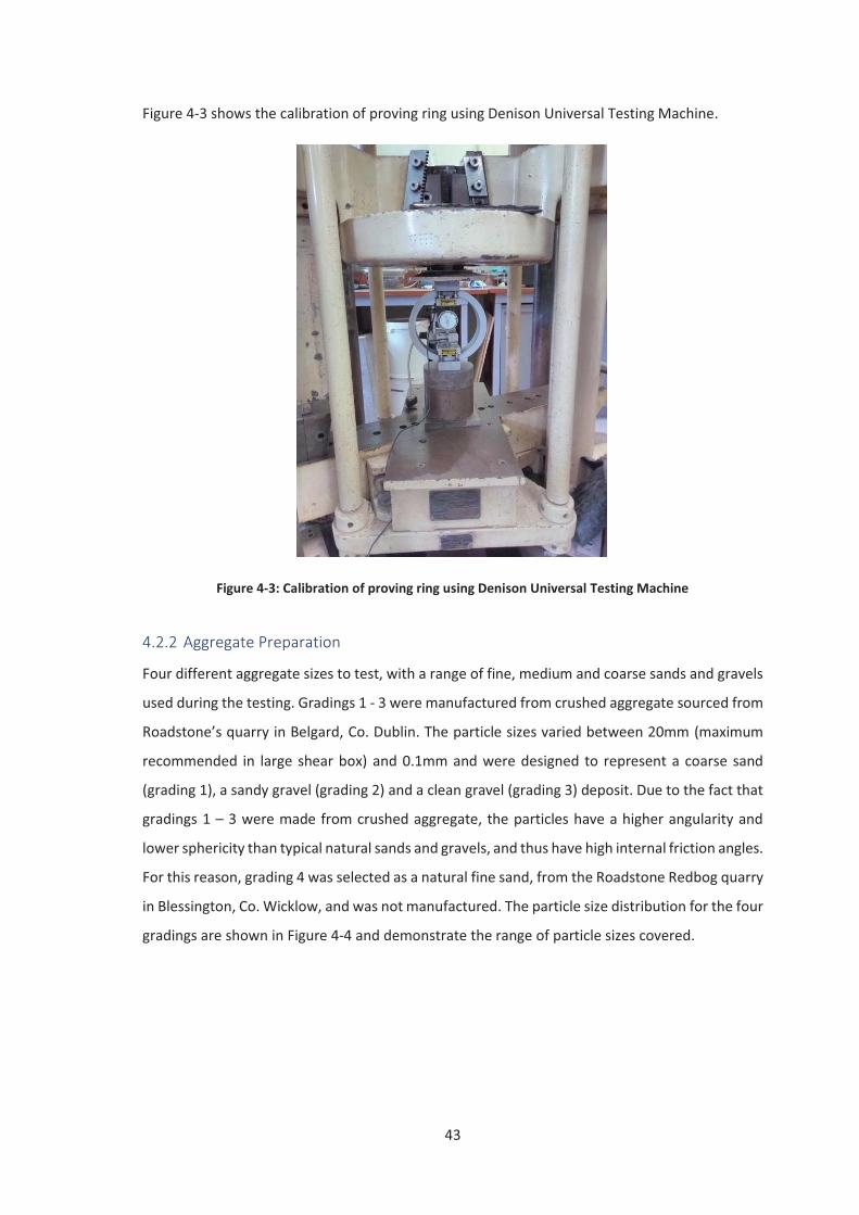
43

Figure 4-3 shows the calibration of proving ring using Denison Universal Testing Machine.

Figure 4-3: Calibration of proving ring using Denison Universal Testing Machine

4.2.2 Aggregate Preparation

Four different aggregate sizes to test, with a range of fine, medium and coarse sands and gravels

used during the testing. Gradings 1 - 3 were manufactured from crushed aggregate sourced from

Roadstone’s quarry in Belgard, Co. Dublin. The particle sizes varied between 20mm (maximum

recommended in large shear box) and 0.1mm and were designed to represent a coarse sand

(grading 1), a sandy gravel (grading 2) and a clean gravel (grading 3) deposit. Due to the fact that

gradings 1 – 3 were made from crushed aggregate, the particles have a higher angularity and

lower sphericity than typical natural sands and gravels, and thus have high internal friction angles.

For this reason, grading 4 was selected as a natural fine sand, from the Roadstone Redbog quarry

in Blessington, Co. Wicklow, and was not manufactured. The particle size distribution for the four

gradings are shown in Figure 4-4 and demonstrate the range of particle sizes covered.

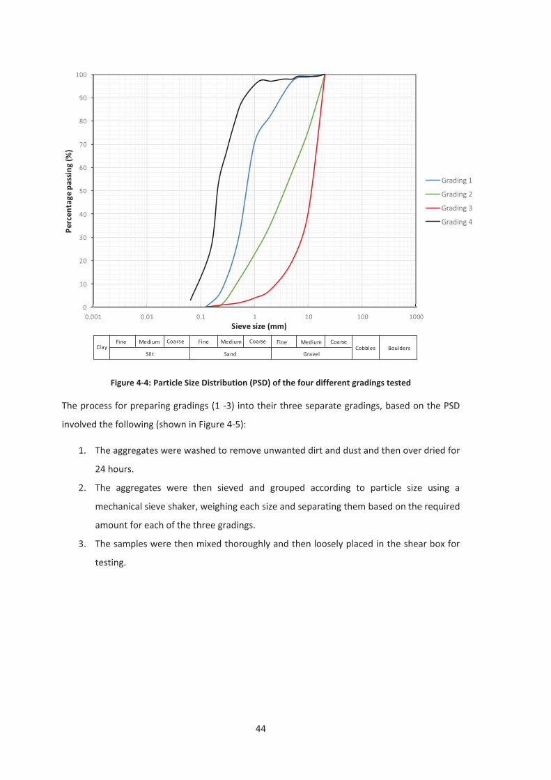
44

Figure 4-4: Particle Size Distribution (PSD) of the four different gradings tested

The process for preparing gradings (1 -3) into their three separate gradings, based on the PSD

involved the following (shown in Figure 4-5):

1. The aggregates were washed to remove unwanted dirt and dust and then over dried for

24 hours.

2. The aggregates were then sieved and grouped according to particle size using a

mechanical sieve shaker, weighing each size and separating them based on the required

amount for each of the three gradings.

3. The samples were then mixed thoroughly and then loosely placed in the shear box for

testing.

0

10

20

30

40

50

60

70

80

90

100

00.001 0.01 0.1 1 10 100 1000

Perc

enta

ge p

assin

g (%

)

Sieve size (mm)

Grading 1

Grading 2

Grading 3

Grading 4

Clay Cobbles BouldersSilt Sand Gravel

Fine Medium Coarse Fine Medium Coarse Fine Medium Coarse

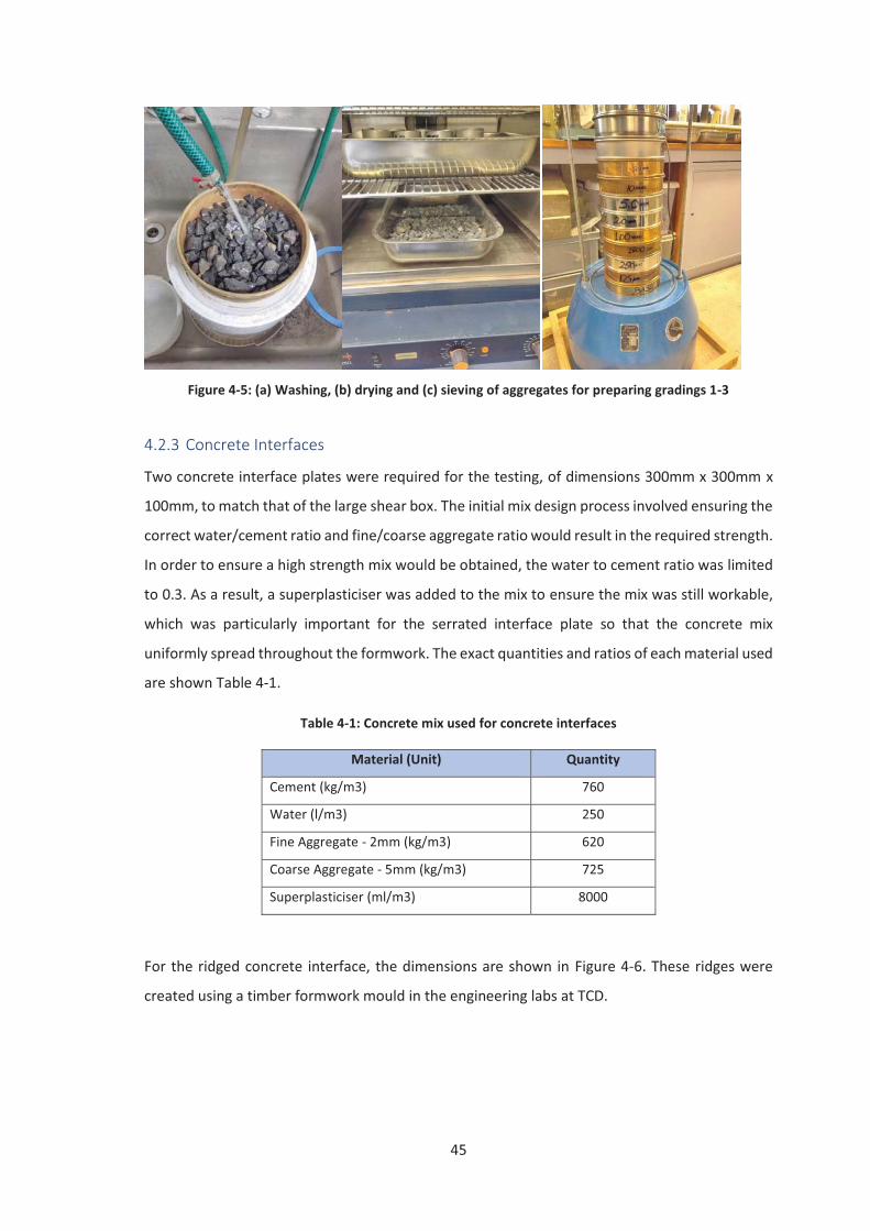
45

Figure 4-5: (a) Washing, (b) drying and (c) sieving of aggregates for preparing gradings 1-3

4.2.3 Concrete Interfaces

Two concrete interface plates were required for the testing, of dimensions 300mm x 300mm x

100mm, to match that of the large shear box. The initial mix design process involved ensuring the

correct water/cement ratio and fine/coarse aggregate ratio would result in the required strength.

In order to ensure a high strength mix would be obtained, the water to cement ratio was limited

to 0.3. As a result, a superplasticiser was added to the mix to ensure the mix was still workable,

which was particularly important for the serrated interface plate so that the concrete mix

uniformly spread throughout the formwork. The exact quantities and ratios of each material used

are shown Table 4-1.

Table 4-1: Concrete mix used for concrete interfaces

Material (Unit) Quantity

Cement (kg/m3) 760

Water (l/m3) 250

Fine Aggregate - 2mm (kg/m3) 620

Coarse Aggregate - 5mm (kg/m3) 725

Superplasticiser (ml/m3) 8000

For the ridged concrete interface, the dimensions are shown in Figure 4-6. These ridges were

created using a timber formwork mould in the engineering labs at TCD.

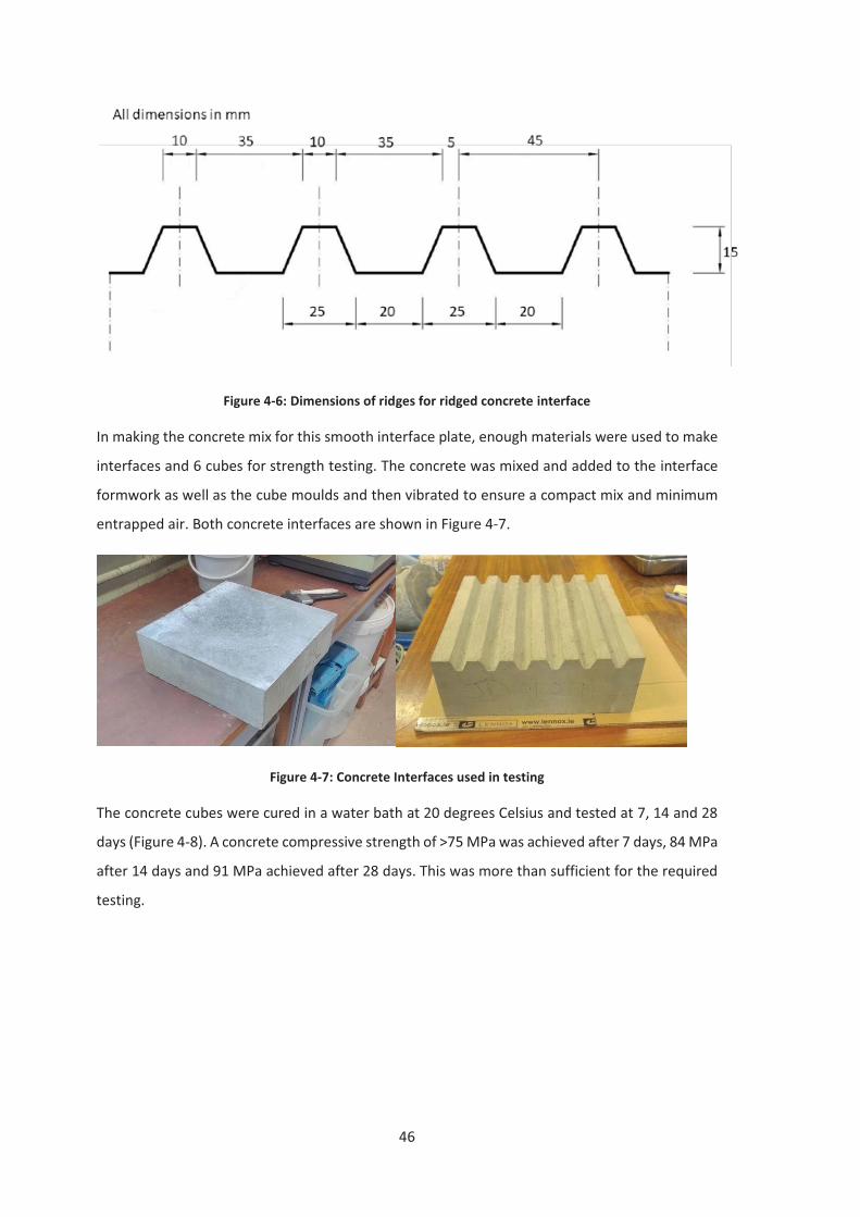
46

Figure 4-6: Dimensions of ridges for ridged concrete interface

In making the concrete mix for this smooth interface plate, enough materials were used to make

interfaces and 6 cubes for strength testing. The concrete was mixed and added to the interface

formwork as well as the cube moulds and then vibrated to ensure a compact mix and minimum

entrapped air. Both concrete interfaces are shown in Figure 4-7.

Figure 4-7: Concrete Interfaces used in testing

The concrete cubes were cured in a water bath at 20 degrees Celsius and tested at 7, 14 and 28

days (Figure 4-8). A concrete compressive strength of >75 MPa was achieved after 7 days, 84 MPa

after 14 days and 91 MPa achieved after 28 days. This was more than sufficient for the required

testing.

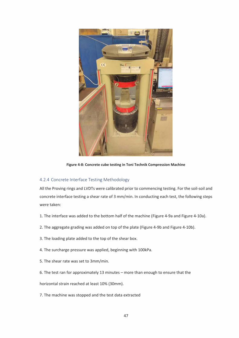
47

Figure 4-8: Concrete cube testing in Toni Technik Compression Machine

4.2.4 Concrete Interface Testing Methodology

All the Proving rings and LVDTs were calibrated prior to commencing testing. For the soil-soil and

concrete interface testing a shear rate of 3 mm/min. In conducting each test, the following steps

were taken:

1. The interface was added to the bottom half of the machine (Figure 4-9a and Figure 4-10a).

2. The aggregate grading was added on top of the plate (Figure 4-9b and Figure 4-10b).

3. The loading plate added to the top of the shear box.

4. The surcharge pressure was applied, beginning with 100kPa.

5. The shear rate was set to 3mm/min.

6. The test ran for approximately 13 minutes – more than enough to ensure that the

horizontal strain reached at least 10% (30mm).

7. The machine was stopped and the test data extracted

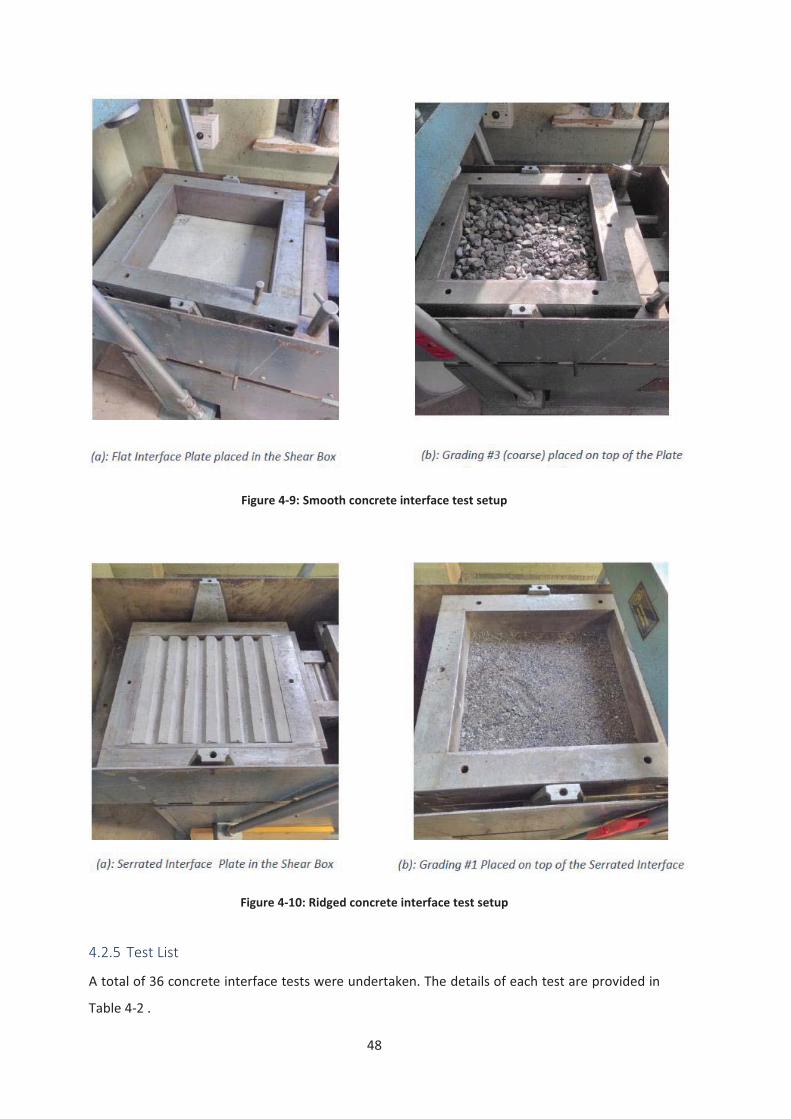
48

Figure 4-9: Smooth concrete interface test setup

Figure 4-10: Ridged concrete interface test setup

4.2.5 Test List

A total of 36 concrete interface tests were undertaken. The details of each test are provided in

Table 4-2 .

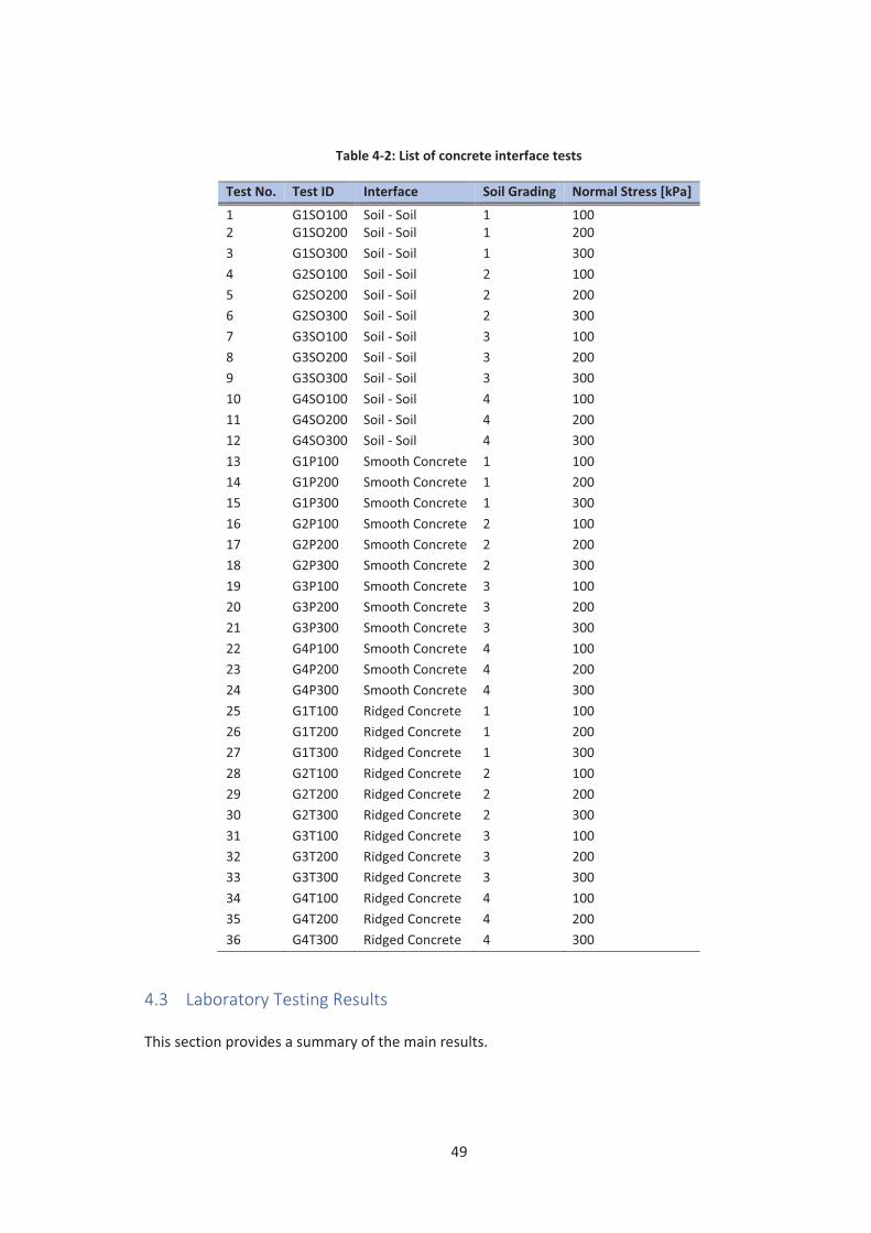
49

Table 4-2: List of concrete interface tests

Test No. Test ID Interface Soil Grading Normal Stress [kPa] 1 G1SO100 Soil - Soil 1 100 2 G1SO200 Soil - Soil 1 200 3 G1SO300 Soil - Soil 1 300 4 G2SO100 Soil - Soil 2 100 5 G2SO200 Soil - Soil 2 200 6 G2SO300 Soil - Soil 2 300 7 G3SO100 Soil - Soil 3 100 8 G3SO200 Soil - Soil 3 200 9 G3SO300 Soil - Soil 3 300 10 G4SO100 Soil - Soil 4 100 11 G4SO200 Soil - Soil 4 200 12 G4SO300 Soil - Soil 4 300 13 G1P100 Smooth Concrete 1 100 14 G1P200 Smooth Concrete 1 200 15 G1P300 Smooth Concrete 1 300 16 G2P100 Smooth Concrete 2 100 17 G2P200 Smooth Concrete 2 200 18 G2P300 Smooth Concrete 2 300 19 G3P100 Smooth Concrete 3 100 20 G3P200 Smooth Concrete 3 200 21 G3P300 Smooth Concrete 3 300 22 G4P100 Smooth Concrete 4 100 23 G4P200 Smooth Concrete 4 200 24 G4P300 Smooth Concrete 4 300 25 G1T100 Ridged Concrete 1 100 26 G1T200 Ridged Concrete 1 200 27 G1T300 Ridged Concrete 1 300 28 G2T100 Ridged Concrete 2 100 29 G2T200 Ridged Concrete 2 200 30 G2T300 Ridged Concrete 2 300 31 G3T100 Ridged Concrete 3 100 32 G3T200 Ridged Concrete 3 200 33 G3T300 Ridged Concrete 3 300 34 G4T100 Ridged Concrete 4 100 35 G4T200 Ridged Concrete 4 200 36 G4T300 Ridged Concrete 4 300

4.3 Laboratory Testing Results

This section provides a summary of the main results.

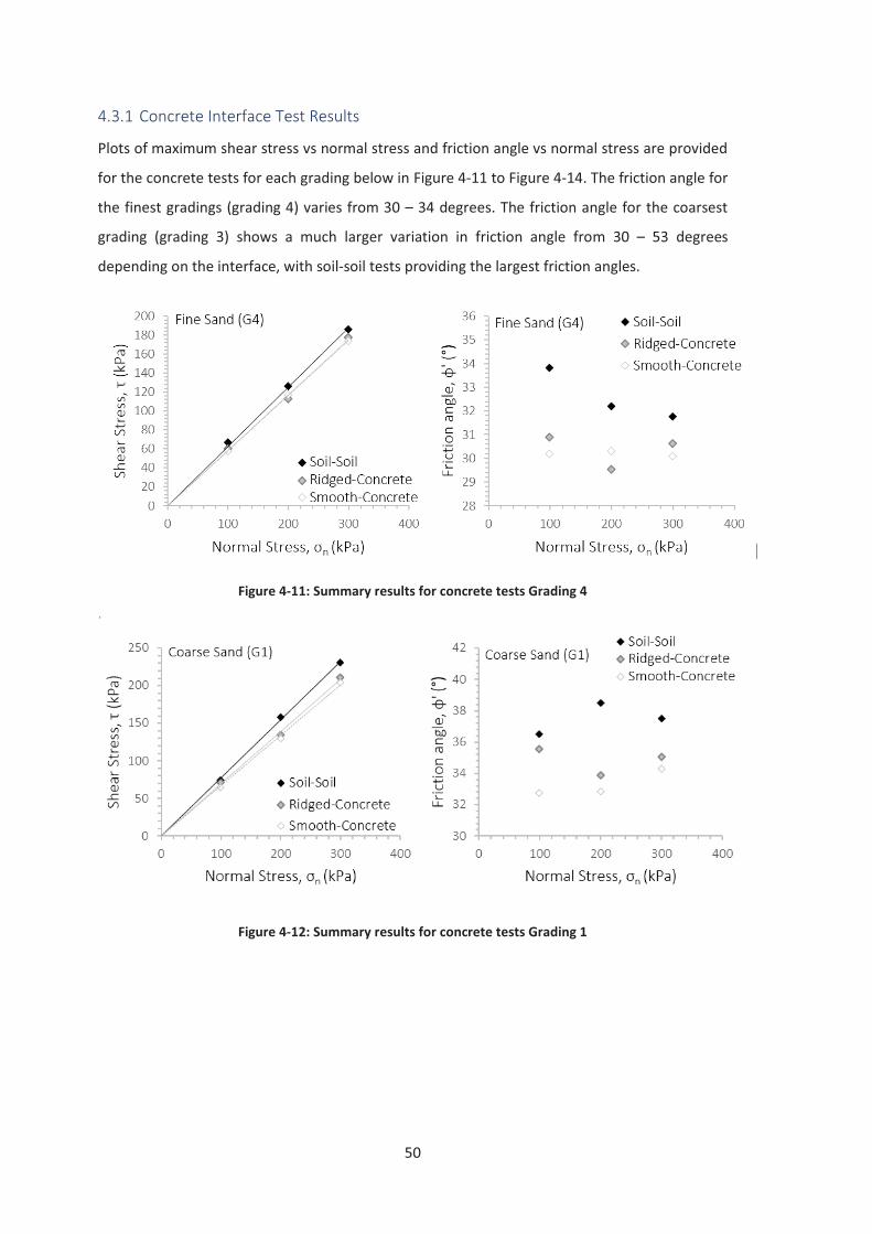
50

4.3.1 Concrete Interface Test Results

Plots of maximum shear stress vs normal stress and friction angle vs normal stress are provided

for the concrete tests for each grading below in Figure 4-11 to Figure 4-14. The friction angle for

the finest gradings (grading 4) varies from 30 – 34 degrees. The friction angle for the coarsest

grading (grading 3) shows a much larger variation in friction angle from 30 – 53 degrees

depending on the interface, with soil-soil tests providing the largest friction angles.

Figure 4-11: Summary results for concrete tests Grading 4

Figure 4-12: Summary results for concrete tests Grading 1

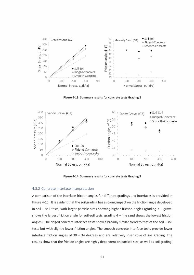
51

Figure 4-13: Summary results for concrete tests Grading 2

Figure 4-14: Summary results for concrete tests Grading 3

4.3.2 Concrete Interface Interpretation

A comparison of the interface friction angles for different gradings and interfaces is provided in

Figure 4-15. It is evident that the soil grading has a strong impact on the friction angle developed

in soil – soil tests, with larger particle sizes showing higher friction angles (grading 3 – gravel

shows the largest friction angle for soil-soil tests, grading 4 – fine sand shows the lowest friction

angles). The ridged concrete interface tests show a broadly similar trend to that of the soil – soil

tests but with slightly lower friction angles. The smooth concrete interface tests provide lower

interface friction angles of 30 – 34 degrees and are relatively insensitive of soil grading. The

results show that the friction angles are highly dependent on particle size, as well as soil grading.

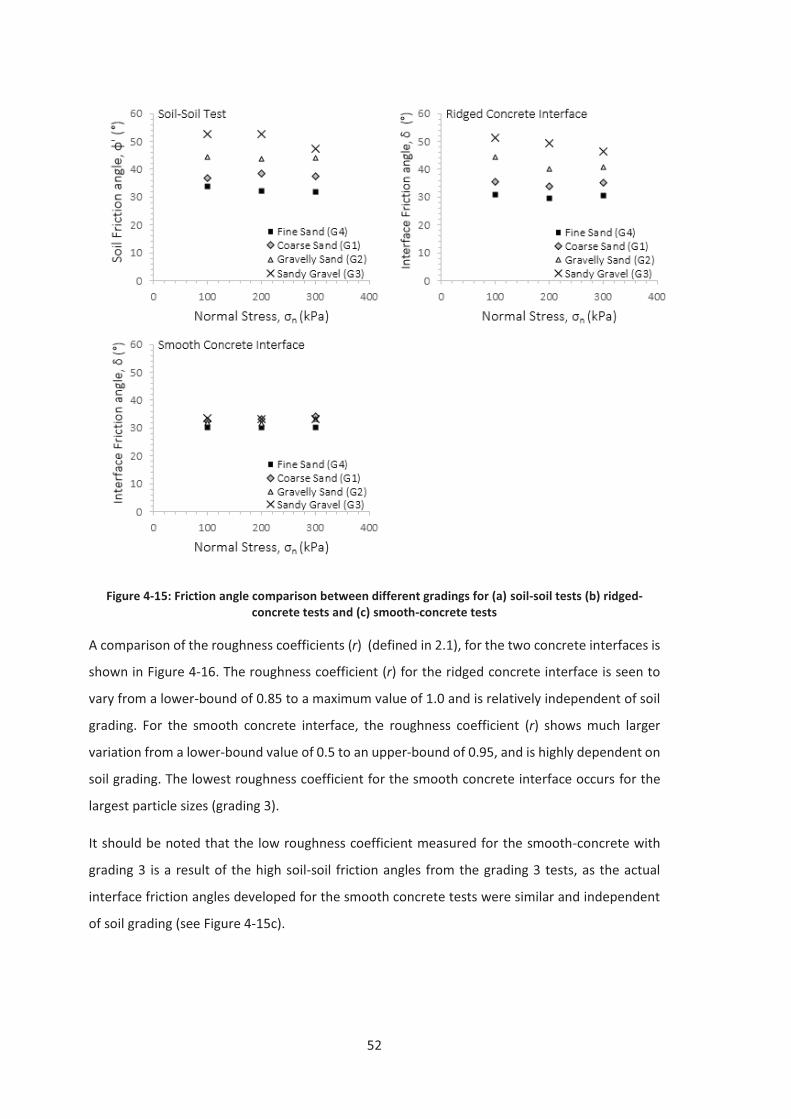
52

Figure 4-15: Friction angle comparison between different gradings for (a) soil-soil tests (b) ridged-concrete tests and (c) smooth-concrete tests

A comparison of the roughness coefficients (r) (defined in 2.1), for the two concrete interfaces is

shown in Figure 4-16. The roughness coefficient (r) for the ridged concrete interface is seen to

vary from a lower-bound of 0.85 to a maximum value of 1.0 and is relatively independent of soil

grading. For the smooth concrete interface, the roughness coefficient (r) shows much larger

variation from a lower-bound value of 0.5 to an upper-bound of 0.95, and is highly dependent on

soil grading. The lowest roughness coefficient for the smooth concrete interface occurs for the

largest particle sizes (grading 3).

It should be noted that the low roughness coefficient measured for the smooth-concrete with

grading 3 is a result of the high soil-soil friction angles from the grading 3 tests, as the actual

interface friction angles developed for the smooth concrete tests were similar and independent

of soil grading (see Figure 4-15c).

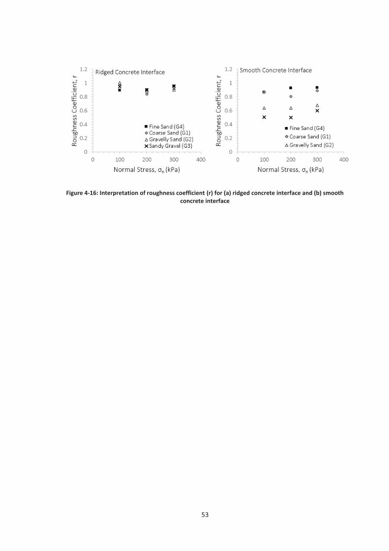
53

Figure 4-16: Interpretation of roughness coefficient (r) for (a) ridged concrete interface and (b) smooth concrete interface

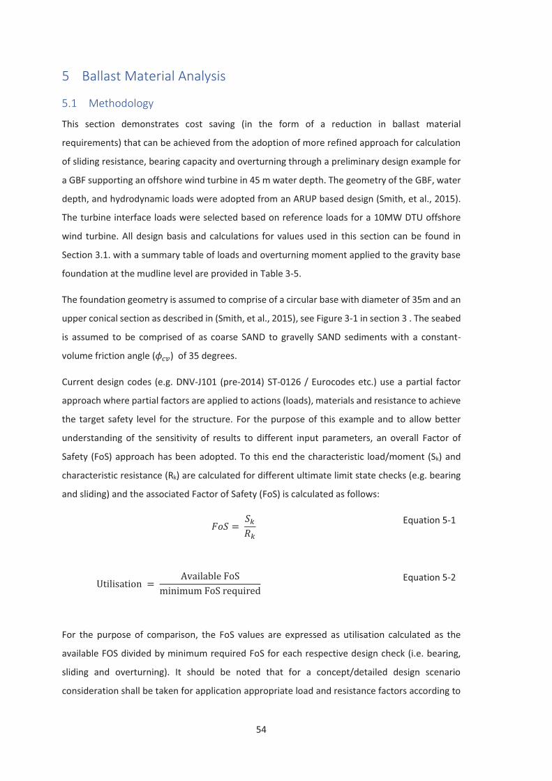
54

5 Ballast Material Analysis

5.1 Methodology

This section demonstrates cost saving (in the form of a reduction in ballast material

requirements) that can be achieved from the adoption of more refined approach for calculation

of sliding resistance, bearing capacity and overturning through a preliminary design example for

a GBF supporting an offshore wind turbine in 45 m water depth. The geometry of the GBF, water

depth, and hydrodynamic loads were adopted from an ARUP based design (Smith, et al., 2015).

The turbine interface loads were selected based on reference loads for a 10MW DTU offshore

wind turbine. All design basis and calculations for values used in this section can be found in

Section 3.1. with a summary table of loads and overturning moment applied to the gravity base

foundation at the mudline level are provided in Table 3-5.

The foundation geometry is assumed to comprise of a circular base with diameter of 35m and an

upper conical section as described in (Smith, et al., 2015), see Figure 3-1 in section 3 . The seabed

is assumed to be comprised of as coarse SAND to gravelly SAND sediments with a constant-

volume friction angle ( ) of 35 degrees.

Current design codes (e.g. DNV-J101 (pre-2014) ST-0126 / Eurocodes etc.) use a partial factor

approach where partial factors are applied to actions (loads), materials and resistance to achieve

the target safety level for the structure. For the purpose of this example and to allow better

understanding of the sensitivity of results to different input parameters, an overall Factor of

Safety (FoS) approach has been adopted. To this end the characteristic load/moment (Sk) and

characteristic resistance (Rk) are calculated for different ultimate limit state checks (e.g. bearing

and sliding) and the associated Factor of Safety (FoS) is calculated as follows:

Equation 5-1

Equation 5-2

For the purpose of comparison, the FoS values are expressed as utilisation calculated as the

available FOS divided by minimum required FoS for each respective design check (i.e. bearing,

sliding and overturning). It should be noted that for a concept/detailed design scenario

consideration shall be taken for application appropriate load and resistance factors according to

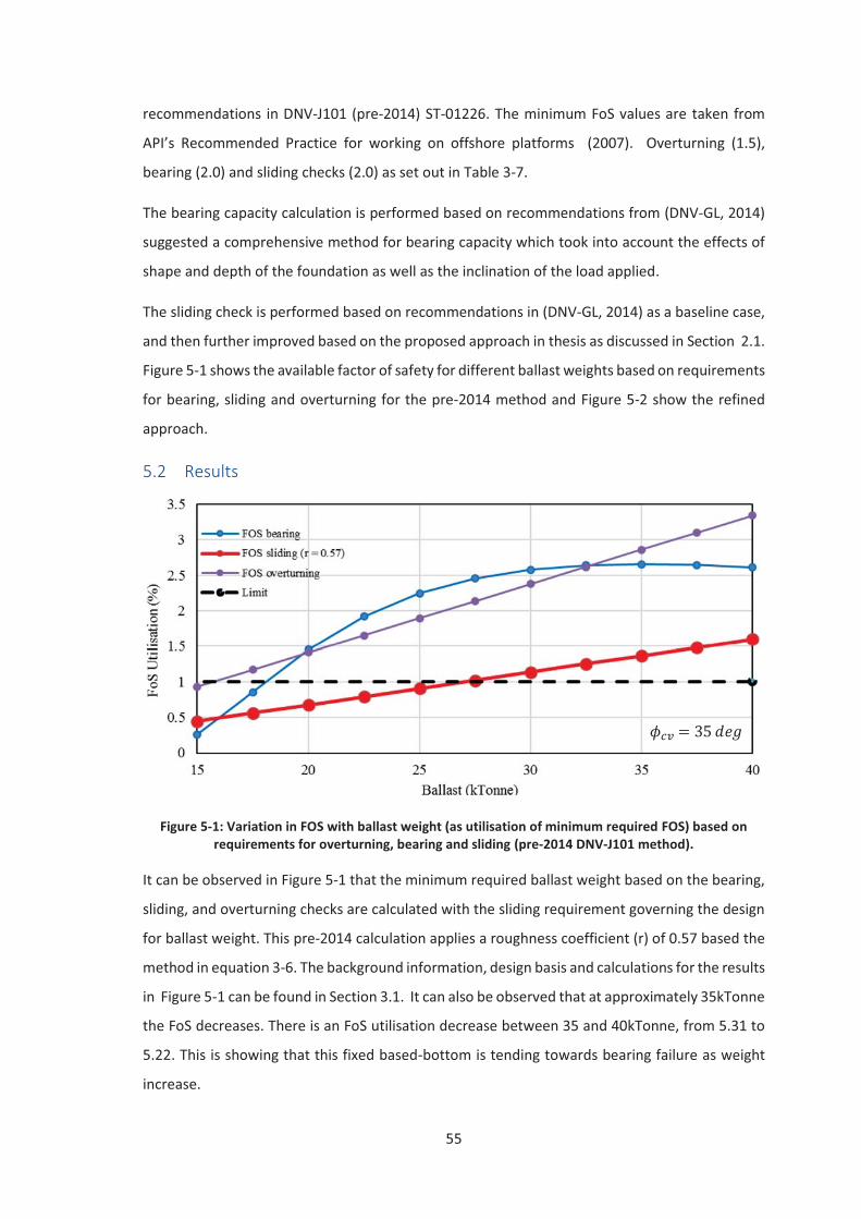
55

recommendations in DNV-J101 (pre-2014) ST-01226. The minimum FoS values are taken from

API’s Recommended Practice for working on offshore platforms (2007). Overturning (1.5),

bearing (2.0) and sliding checks (2.0) as set out in Table 3-7.

The bearing capacity calculation is performed based on recommendations from (DNV-GL, 2014)

suggested a comprehensive method for bearing capacity which took into account the effects of

shape and depth of the foundation as well as the inclination of the load applied.

The sliding check is performed based on recommendations in (DNV-GL, 2014) as a baseline case,

and then further improved based on the proposed approach in thesis as discussed in Section 2.1.

Figure 5-1 shows the available factor of safety for different ballast weights based on requirements

for bearing, sliding and overturning for the pre-2014 method and Figure 5-2 show the refined

approach.

5.2 Results

Figure 5-1: Variation in FOS with ballast weight (as utilisation of minimum required FOS) based on requirements for overturning, bearing and sliding (pre-2014 DNV-J101 method).

It can be observed in Figure 5-1 that the minimum required ballast weight based on the bearing,

sliding, and overturning checks are calculated with the sliding requirement governing the design

for ballast weight. This pre-2014 calculation applies a roughness coefficient (r) of 0.57 based the

method in equation 3-6. The background information, design basis and calculations for the results

in Figure 5-1 can be found in Section 3.1. It can also be observed that at approximately 35kTonne

the FoS decreases. There is an FoS utilisation decrease between 35 and 40kTonne, from 5.31 to

5.22. This is showing that this fixed based-bottom is tending towards bearing failure as weight

increase.

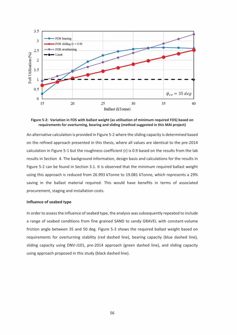
56

Figure 5-2: Variation in FOS with ballast weight (as utilisation of minimum required FOS) based on requirements for overturning, bearing and sliding (method suggested in this MAI project)

An alternative calculation is provided in Figure 5-2 where the sliding capacity is determined based

on the refined approach presented in this thesis, where all values are identical to the pre-2014

calculation in Figure 5-1 but the roughness coefficient (r) is 0.9 based on the results from the lab

results in Section 4. The background information, design basis and calculations for the results in

Figure 5-2 can be found in Section 3.1. It is observed that the minimum required ballast weight

using this approach is reduced from 26.993 kTonne to 19.081 kTonne, which represents a 29%

saving in the ballast material required. This would have benefits in terms of associated

procurement, staging and installation costs.

Influence of seabed type

In order to assess the influence of seabed type, the analysis was subsequently repeated to include

a range of seabed conditions from fine grained SAND to sandy GRAVEL with constant-volume

friction angle between 35 and 50 deg. Figure 5-3 shows the required ballast weight based on

requirements for overturning stability (red dashed line), bearing capacity (blue dashed line),

sliding capacity using DNV-J101, pre-2014 approach (green dashed line), and sliding capacity

using approach proposed in this study (black dashed line).

57

Figure 5-3: Comparison of the required ballast weight based on overturning, bearing, and sliding criteria using industry standard DNV-J101 (pre-2014) approach and also the approach proposed in this

study

It can be observed that the sliding capacity calculated using old DNV-J101 (pre-2014) approach

governs the design of ballast weight for all friction angles considered. It is also observed that the

adoption of approach proposed in this study can significantly reduce the required ballast for the

range of friction angles considered. The revised sliding capacity still governs the ballast

requirement in this example for friction angles less than 43 deg. However, for higher friction

angles, the overturning criterion dominates and no further reduction in ballast as a result of

adoption of refined sliding formulation can be realised.

10

12

14

16

18

20

22

24

26

28

30

35 37 39 41 43 45 47 49

Ballast

req

uir

ed

, k

To

nn

es

Soil Friction Angle (φ'cv)

Sliding (This Study)

Overturning

Bearing

Sliding (DNV-J101, pre-2014)

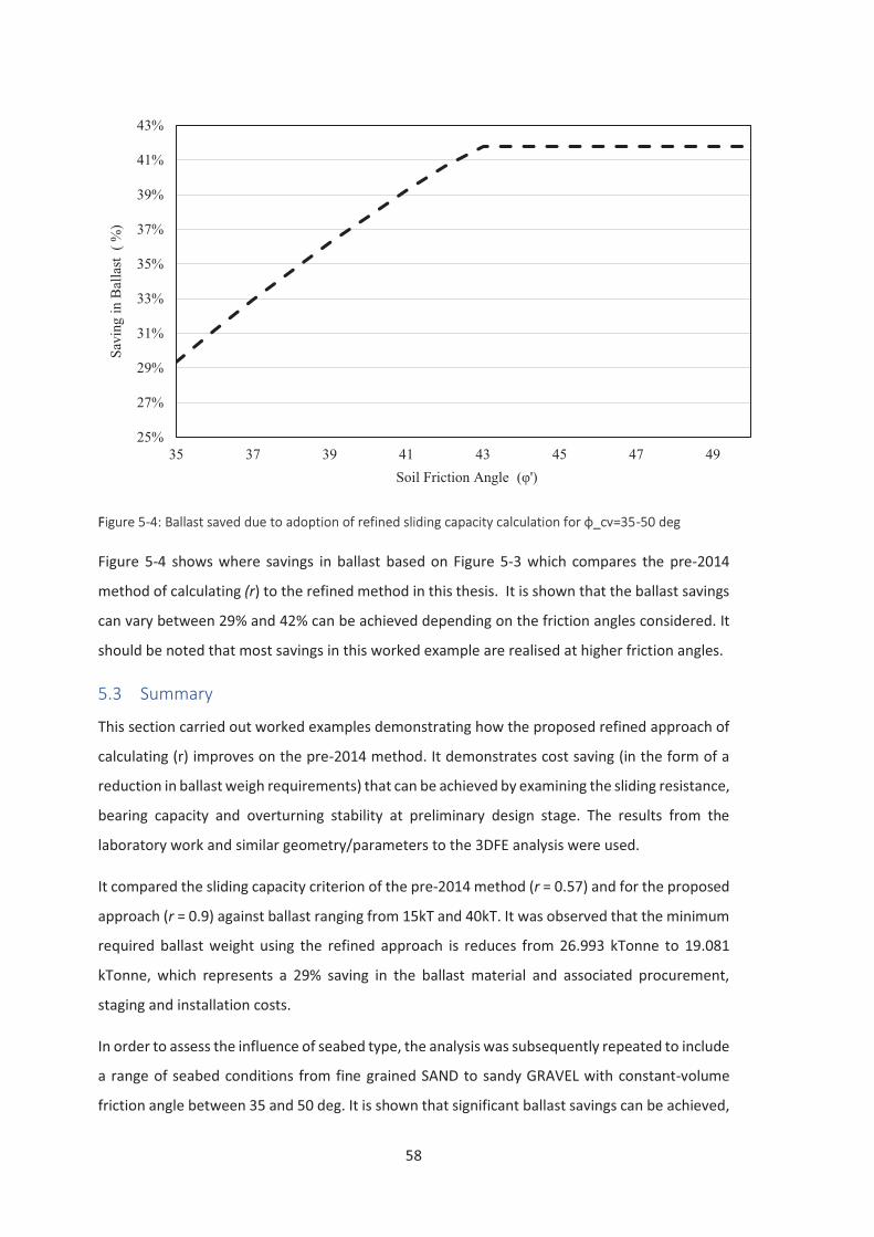
58

FFigure 5-4: Ballast saved due to adoption of refined sliding capacity calculation for ϕ_cv=35-50 deg

Figure 5-4 shows where savings in ballast based on Figure 5-3 which compares the pre-2014

method of calculating (r) to the refined method in this thesis. It is shown that the ballast savings

can vary between 29% and 42% can be achieved depending on the friction angles considered. It

should be noted that most savings in this worked example are realised at higher friction angles.

5.3 Summary

This section carried out worked examples demonstrating how the proposed refined approach of

calculating (r) improves on the pre-2014 method. It demonstrates cost saving (in the form of a

reduction in ballast weigh requirements) that can be achieved by examining the sliding resistance,

bearing capacity and overturning stability at preliminary design stage. The results from the

laboratory work and similar geometry/parameters to the 3DFE analysis were used.

It compared the sliding capacity criterion of the pre-2014 method (r = 0.57) and for the proposed

approach (r = 0.9) against ballast ranging from 15kT and 40kT. It was observed that the minimum

required ballast weight using the refined approach is reduces from 26.993 kTonne to 19.081

kTonne, which represents a 29% saving in the ballast material and associated procurement,

staging and installation costs.

In order to assess the influence of seabed type, the analysis was subsequently repeated to include

a range of seabed conditions from fine grained SAND to sandy GRAVEL with constant-volume

friction angle between 35 and 50 deg. It is shown that significant ballast savings can be achieved,

25%

27%

29%

31%

33%

35%

37%

39%

41%

43%

35 37 39 41 43 45 47 49

Sav

ing i

n B

alla

st

( %

)

Soil Friction Angle (φ')

59

vary between 29% and 42% can be achieved depending on the friction angles considered. It

should be noted that most savings in this example are realised at higher friction angles. The

revised sliding capacity still governs the ballast requirement in this example for friction angles

less than 43 deg. However, for higher friction angles, the overturning criterion dominates and no

further reduction in ballast as a result of adoption of refined sliding formulation can be realised.

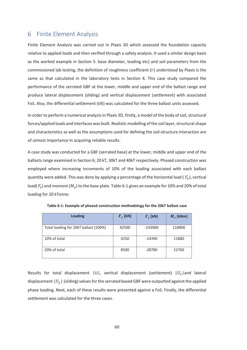
60

6 Finite Element Analysis

Finite Element Analysis was carried out in Plaxis 3D which assessed the foundation capacity

relative to applied loads and then verified through a safety analysis. It used a similar design basis

as the worked example in Section 5. base diameter, loading etc) and soil parameters from the

commissioned lab testing, the definition of roughness coefficient ( ) understood by Plaxis is the

same as that calculated in the laboratory tests in Section 4. This case study compared the

performance of the serrated GBF at the lower, middle and upper end of the ballast range and

produce lateral displacement (sliding) and vertical displacement (settlement) with associated

FoS. Also, the differential settlement (tilt) was calculated for the three ballast units assessed.

In order to perform a numerical analysis in Plaxis 3D, firstly, a model of the body of soil, structural

forces/applied loads and interfaces was built. Realistic modelling of the soil layer, structural shape

and characteristics as well as the assumptions used for defining the soil-structure interaction are

of utmost importance in acquiring reliable results.

A case study was conducted for a GBF (serrated base) at the lower, middle and upper end of the

ballasts range examined in Section 6; 20 kT, 30kT and 40kT respectively. Phased construction was

employed where increasing increments of 10% of the loading associated with each ballast

quantity were added. This was done by applying a percentage of the horizontal load ( ), vertical

load( ) and moment ( ) to the base plate. Table 6-1 gives an example for 10% and 20% of total

loading for 20 kTonne.

Table 6-1: Example of phased construction methodology for the 20kT ballast case

Loading [kN] [kN] [kNm]

Total loading for 20kT ballast (100%) 42500 -143900 118800

10% of total 4250 -14390 11880

20% of total 8500 -28780 23760

Results for total displacement |U|, vertical displacement (settlement) | |and lateral

displacement | | (sliding) values for the serrated based GBF were outputted against the applied

phase loading. Next, each of these results were presented against a FoS. Finally, the differential

settlement was calculated for the three cases.

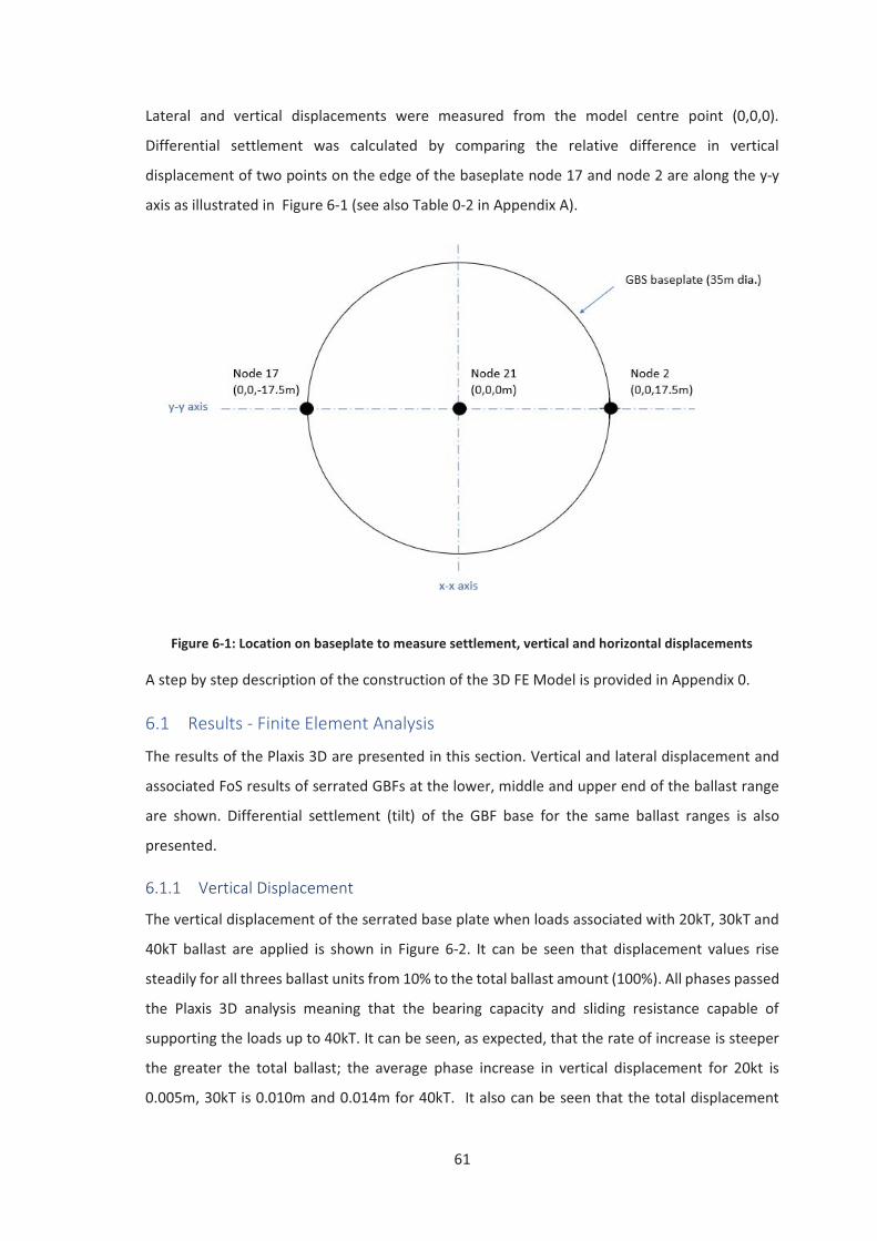
61

Lateral and vertical displacements were measured from the model centre point (0,0,0).

Differential settlement was calculated by comparing the relative difference in vertical

displacement of two points on the edge of the baseplate node 17 and node 2 are along the y-y

axis as illustrated in Figure 6-1 (see also Table 0-2 in Appendix A).

Figure 6-1: Location on baseplate to measure settlement, vertical and horizontal displacements

A step by step description of the construction of the 3D FE Model is provided in Appendix 0.

6.1 Results - Finite Element Analysis

The results of the Plaxis 3D are presented in this section. Vertical and lateral displacement and

associated FoS results of serrated GBFs at the lower, middle and upper end of the ballast range

are shown. Differential settlement (tilt) of the GBF base for the same ballast ranges is also

presented.

6.1.1 Vertical Displacement

The vertical displacement of the serrated base plate when loads associated with 20kT, 30kT and

40kT ballast are applied is shown in Figure 6-2. It can be seen that displacement values rise

steadily for all threes ballast units from 10% to the total ballast amount (100%). All phases passed

the Plaxis 3D analysis meaning that the bearing capacity and sliding resistance capable of

supporting the loads up to 40kT. It can be seen, as expected, that the rate of increase is steeper

the greater the total ballast; the average phase increase in vertical displacement for 20kt is

0.005m, 30kT is 0.010m and 0.014m for 40kT. It also can be seen that the total displacement

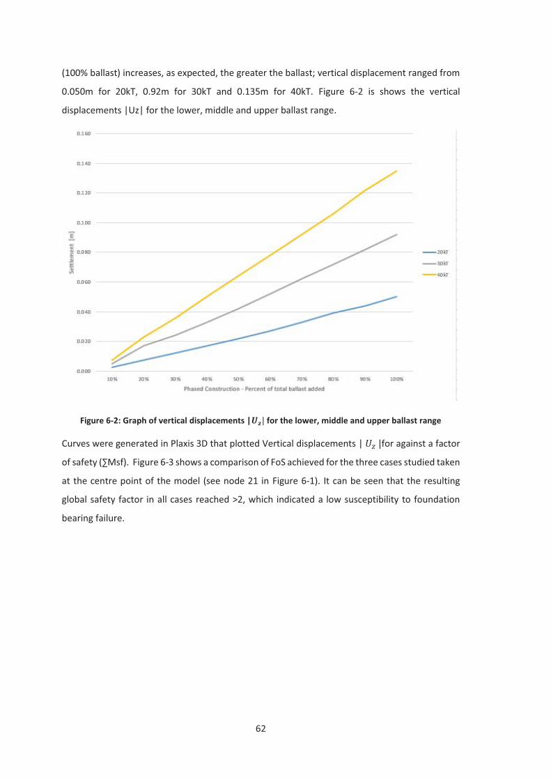
62

(100% ballast) increases, as expected, the greater the ballast; vertical displacement ranged from

0.050m for 20kT, 0.92m for 30kT and 0.135m for 40kT. Figure 6-2 is shows the vertical

displacements |Uz| for the lower, middle and upper ballast range.

Figure 6-2: Graph of vertical displacements | for the lower, middle and upper ballast range

Curves were generated in Plaxis 3D that plotted Vertical displacements | for against a factor

of safety (∑Msf). Figure 6-3 shows a comparison of FoS achieved for the three cases studied taken

at the centre point of the model (see node 21 in Figure 6-1). It can be seen that the resulting

global safety factor in all cases reached >2, which indicated a low susceptibility to foundation

bearing failure.

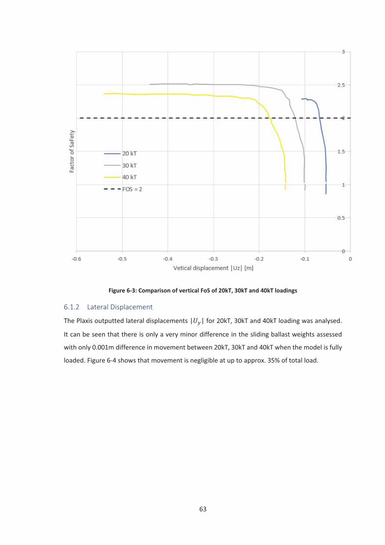
63

Figure 6-3: Comparison of vertical FoS of 20kT, 30kT and 40kT loadings

6.1.2 Lateral Displacement

The Plaxis outputted lateral displacements | | for 20kT, 30kT and 40kT loading was analysed.

It can be seen that there is only a very minor difference in the sliding ballast weights assessed

with only 0.001m difference in movement between 20kT, 30kT and 40kT when the model is fully

loaded. Figure 6-4 shows that movement is negligible at up to approx. 35% of total load.

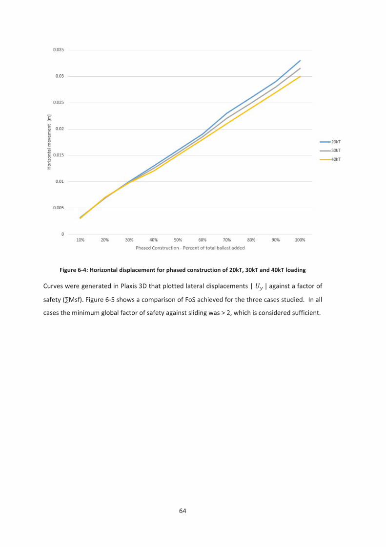
64

Figure 6-4: Horizontal displacement for phased construction of 20kT, 30kT and 40kT loading

Curves were generated in Plaxis 3D that plotted lateral displacements | against a factor of

safety (∑Msf). Figure 6-5 shows a comparison of FoS achieved for the three cases studied. In all

cases the minimum global factor of safety against sliding was > 2, which is considered sufficient.

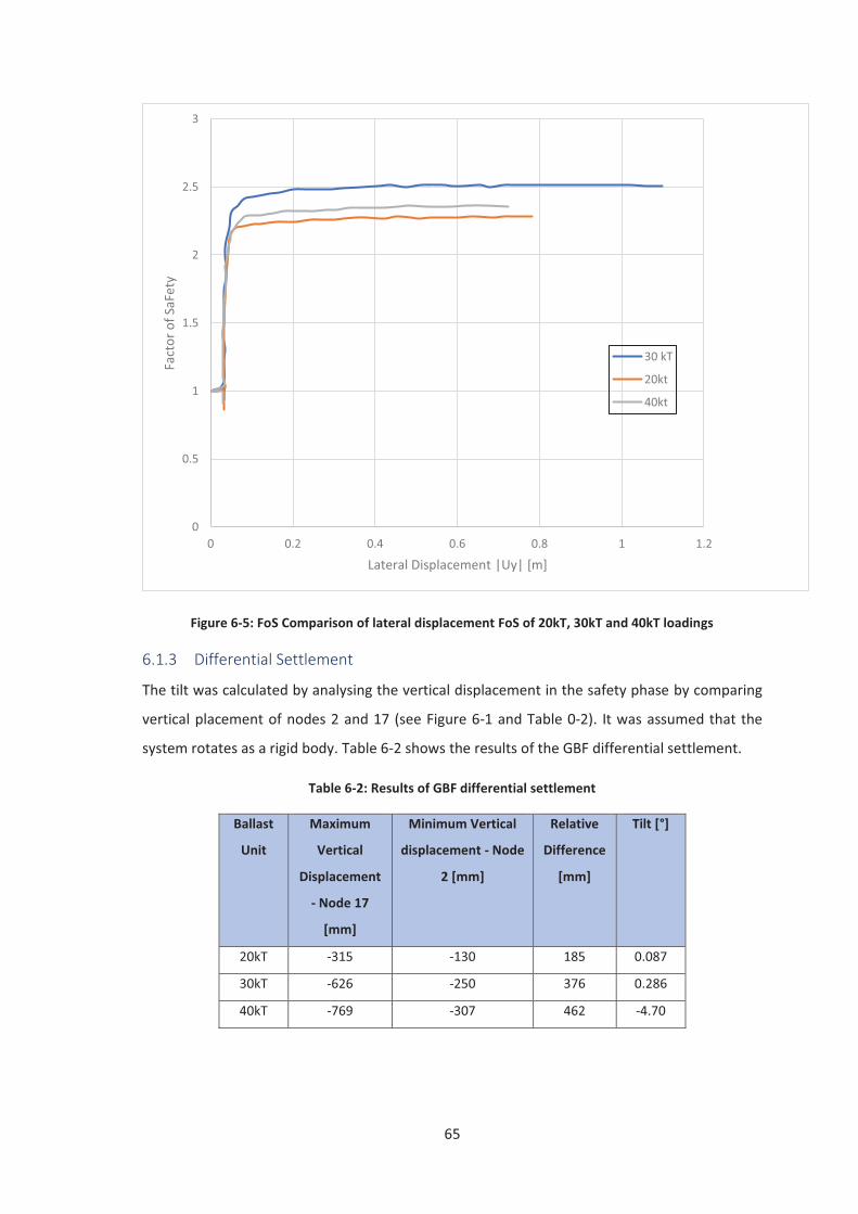
65

Figure 6-5: FoS Comparison of lateral displacement FoS of 20kT, 30kT and 40kT loadings

6.1.3 Differential Settlement

The tilt was calculated by analysing the vertical displacement in the safety phase by comparing

vertical placement of nodes 2 and 17 (see Figure 6-1 and Table 0-2). It was assumed that the

system rotates as a rigid body. Table 6-2 shows the results of the GBF differential settlement.

Table 6-2: Results of GBF differential settlement

Ballast

Unit

Maximum

Vertical

Displacement

- Node 17

[mm]

Minimum Vertical

displacement - Node

2 [mm]

Relative

Difference

[mm]

Tilt [°]

20kT -315 -130

185

0.087

30kT -626 -250 376 0.286

40kT -769 -307 462 -4.70

0

0.5

1

1.5

2

2.5

3

0 0.2 0.4 0.6 0.8 1 1.2

Fact

or o

f SaF

ety

Lateral Displacement |Uy| [m]

30 kT

20kt

40kt

66

The result show that the loading of 20kT is within the tilt tolerance of 0.25°, 30 kT is marginally

outside while 40kT is significantly out of tolerance.

67

7 Discussion

The central question of this thesis is to explore if efficiencies can be achieved in the design of

gravity-based foundation (GBF) for offshore wind turbines and if a reduction in quantity of

material required to ballast the structure is possible. It did this through a refinement to the

current method of calculating sliding resistance and demonstrates this through a series of

analyses that offer solutions to gaps in knowledge on this topic.

After the proposed refined approach to calculate the roughness coefficient (r) is put forward in

Section 2.1 three separate exercise were carried out to expand upon it. Laboratory testing

(commissioned work) that provided data to produce interpretations of friction and interface

friction angles, ballast material requirement that compared the pre-2014 DNV method of

quantifying ballast quantities to the refined method and a FEA analysis that quantified vertical

and lateral displacements for a serrated base. The lab work provided roughness values (r) for the

analytical and the FE studies.

Section 2.1 provides a background to the design codes and the development of the methods used

to calculate sliding resistance. To help provide clarity to the industry an alternative was sought

into how the roughness coefficient ( ) is calculated; this thesis suggests an alternative approach

to try fill this gap in knowledge in GBFs design. The tan of the interface friction angle (

divided by the tan of the soils internal friction angle ( ) as outlined in equation 2-8 is

proposed as a formula to calculate . By applying this formula to lab. results a more accurate

estimate of was calculated for the range of soils and interface type tested.

The commissioned laboratory testing provided good raw geotechnical data to aid this thesis. It

produced similar results for gradings 1-3 to Dunne’s testing (2019) and added in a fourth grading

(fine sand from Blessington) at the request of the author of this thesis which Doherty et al.

suggests has similar characteristic to specific to Irish Sea offshore sites (Doherty, et al., 2012).

The roughness coefficients (r) calculated from the results are a vital piece of data for the refined

formula which permitted completion of the ballast calculations (Section 5) and Plaxis modelling

(Section 6) .The results provide new light on the variation of friction angles for soil on soil,

serrated and smooth tests was large for coarse soil e.g. they ranged from 30 to 53 for coarse grain

soils (G3) whereas the was less variation for Blessington Sand (G4).

Another potential use of the lab. results and possible additional study could be to calculate API

sliding resistance (API method) outlined section 2.1. The lab results produced a range of soils

68

internal friction angles that could be applied to equation 2-2. This would allow a direct

comparison of the API and DNV methods.

A ballast requirement analysis was carried out to demonstrate to industry how the refined sliding

resistance calculation can lead to greater efficiencies in GBF design. The analysis showed how a

29% saving in ballast can be achieved; it was observed that the minimum required ballast weight

using this approach is reduced from 26.993 kTonne to 19.081 kTonne, a saving of almost 8

kTonne. It also provides likely savings in ballast required for a range of seabed conditions (fine

grained SAND to sandy GRAVEL). It concludes sliding capacity still governs design for friction

angles below 43°; above this value overturning is the governing factor and no ballast savings can

be achieved. This give developers a clear template to base early stage design and can be adapted

to other offshore renewables sectors i.e. tidal and wave employing a similar foundation type.

Analysis in Plaxis 3D shows that with increased loading the vertical displacement increases; a 20

kTonne results in a 50mm, 30 kTonne equates to 92mm and 40 kTonne results in a 104mm within

the permitted FoS, thus proving that the bearing capacity is sufficient in Blessington Sand to

support the fully ballasted GBF. While some lateral displacement took place (average 31.5mm),

it was insensitive to the ballast quantity tested. This was expected for a structure of such weight

and vertical loading.

Due to the large loads being applied in the vertical direction the small saw-tooth serration (70mm

deep in Demogravi3 project and 15mm in lab testing) offered certain amount of sliding resistance.

Perhaps further testing on a courser material (e.g. grading 3 in the lab section has an -value of

0.58) could show a reduction in sliding resistance. A serrated base interface cannot be considered

in the same category as piles or skirting which penetrate meters into the seabed. In the analysis

carried out by Attari (2016) where piles were compared to a flat base (without piles) there was

significant decrease in lateral movement with piles.

Tilt was checked at the end of the FEA section. It showed that only the differential settlement

associated with the 20 kTonne ballasted GBF (ΔS = 185 mm) was within the tilt tolerance of 0.25°,

30 kTonne was just outside tolerance and 40 k Tonne would mean failure with a tilt of 4.7°. The

installing a flat bed of gravel in sufficient quantities help reduce tilt of these last two cases would

be required, this has been the procedure in most installations to date.

It was the author’s intention to study a soil typical to Irish sea conditions, hence, Blessington Sand

(fine SAND) was added to the lab experiments (grading 4) which provides the roughness

parameter (r) used in in Plaxis; the ground model was designed accordingly with a friction angle

69

of 35° assigned to the ground model based on the (Igoe & Gavin, 2019); however, the laboratory

testing produced a lower friction angle ( average of 30.5°) for the serrated base. The Plaxis results

may not have been as favourable if this lower value were used.

The water depth (45m) selected was deeper than any installation to date and is very much looking

to the future with the trend set to continue into deeper waters. The diameter (35m) was used for

both analytical analysis and the FEA analysis and should be considered general; in practice, in

early stage design the diameter would be varied to meet bearing, sliding and overturning to fall

within the required FoS.

New understanding to the calculation of sliding and bearing capacities have been developed in

this thesis and can be of use to the offshore sector and all aspects of this these helps to link the

gap in the interpretation. However, the Plaxis 3D analysis could have looked at a wider range of

ballasts and a wider range to soils (friction angles of 30 to 50°) and an expansion of this economic

savings showing estimates for financial savings installation time, staging etc. is further work that

can be done.

In conclusion, the thesis achieved its objectives as stated in Section 2.4. This discussion outlined

why the research undertaken in this thesis is relevant, consolidated the findings and allowed for

in-depth comparisons between all of the tests. It highlights gaps in current and past design codes,

proposes refined approach and proceeds to expands on methods to obtain the roughness

coefficient (r), apply, test and prove its validity. This study was carried out specifically for offshore

wind (using a soon to be standard turbine size of 10MW). However, a reduction in ballast

requirements can be applied to other offshore renewables sectors e.g. foundations for tidal

devices.

During detailed design, a project must consider how the specific site characteristics affect the

behaviour of the wind turbine and its support structure. Though the sliding capacity is considered

an ultimate limit state, the load response behaviour of the interface between the foundation and

the soil should also be considered. The results from the laboratory testing, may be considered

during the assessment of the foundation’s load response behaviour in terms of both frequency

assessment and the foundation response as modelled during the analysis of the turbine.

70

8 Conclusion

Offshore wind energy production is set to expand globally into the future. As installations extend

into different seabed conditions and deeper waters all foundation types will find their niche. The

use of GBFs, although only 3.3% of the current installed fleet is due increase to 8.4% in the coming

years.

The central question of this thesis was to explore if efficiencies can be achieved in the design of

gravity-based foundation (GBF) for offshore wind turbines and if a reduction in quantity of

material required to ballast the structure is possible. It did this through a refinement to the

current method of calculating sliding resistance and demonstrates this through a series of

analyses that offer solutions to gaps in knowledge on this topic.

The work contained herein have fulfilled the objectives of the thesis, which were to:

- Develop an equation based on previous studies to estimate the roughness coefficient (r).

- Analyse and interpret laboratory experimental results (commissioned work in Section 4)

to establish the roughness coefficients (using equation proposed in Section 2.1) for flat-

based and serrated bottoms for range of typical offshore seabed types;

- Determine the reduction in ballast material required from adoption of more refined

approach for calculation of sliding resistance (compared to pre-2014 DNV method) based

on experimental testing (analytical calculations in Section 5);

- Carry out stability checks by establishing vertical and lateral displacements along with

differential settlement for the GBF in Blessington Soil using a 3DFE software (Section 6).

This thesis commenced with a comprehensive background into use of GBF in the offshore wind

industry. It sets out the design challenges facing developers that choose a GBF option and outlines

some gaps in the designs codes where there is scope to become more efficient i.e. save in

material usage.

The proposed refined method to calculate the roughness coefficient (r) is put forward and three

separate exercise were carried out to build on this approach; lab experimentation, hand

calculations and FE analysis.

Laboratory testing (commissioned work) that provided data to produce interpretations of friction

and interface friction angles, analytical analysis that compared the pre-2014 DNV method of

quantifying ballast quantities to the refined method suggested in this thesis. The variation of

friction angles for soil on soil, serrated and smooth tests was large for coarse soil e.g. they ranged

from 30 to 53 for coarse grain soils (G3) whereas the was less variation for Blessington Sand (G4).

71

It was observed that the sliding capacity calculated using old DNV-J101 (pre-2014) approach

governs the design of ballast weight for all friction angles considered. It is also observed that the

adoption of approach proposed in this study can significantly reduce the required ballast for the

range of friction angles considered. The hand calculations showed that the minimum required

ballast weight using this approach is reduced from 26.993 kTonne to 19.081 kTonne, which

represents a 29% saving in the ballast material and associated procurement, staging and

installation costs. The revised sliding capacity still governs the ballast requirement in this example

for friction angles less than 43 deg. However, for higher friction angles, the overturning criterion

dominates and no further reduction in ballast as a result of adoption of refined sliding formulation

can be realised.

Finally, the FE analysis produced vertical and lateral displacements for the GBF assessed in Section

6) along with differential settlement for a GBF in Blessington Sand. Analysis in Plaxis 3D shows

that with increased loading the vertical displacement increases; a 20kTonne results in a 50mm,

30kTonne equates to 92mm and 40kTonne results in a 104mm within the permitted FoS, thus

proving that the bearing capacity is sufficient in Blessington Sand to support the fully ballasted

GBF. While some lateral displacement took place (average 31.5mm), it was insensitive to the

ballast quantity tested. This was expected for a structure of such weight and vertical loading.

All elements of this thesis combined helped to demonstrate that through a refinement of the

design approach to sliding resistance, reliable geotechnical data relating to soil and interface

friction angles, early stage estimates of ballast requirement and application of advanced FE

analysis a significant savings can be achieved in offshore wind turbine installation employing a

GBFs.

72

References

4COffshore, 2018. 4C offshore. [Online]

Available at: https://www.4coffshore.com/gravitybasedfoundations

[Accessed 10 October 2018].

Ahmadi, M. & Ghazavi, M., 2012. Effect of Skirt Geometry Variation On Uplift Capacity of Skirted

Foundation, Rhodes, Greece: Proceedings of the International Offshore and Polar Engineering

Conference.

API, 2007. Recommended Practice for Planning, Designing and Constructing Fixed Offshore

Platforms—Working Stress Design, Washington: American Petroleum Institute.

API, 2011. API-RP-2GEO Geotechnical and Foundation Design Considerations, Washington:

American Petroleum Institute.

Attari, A. et al., 2014. LEANWIND Deliverable D3.1 - Novel Vessels and Equipment, Brussels:

European Union’s Seventh Programme for research, technological development and

demonstration .

Attari, Y., 2016. Performance Testing of a Novel Gravity Base Foundation for Offshore Wind,

Dublin: University College Dublin.

Bak, C. et al., 2013. DTU Wind Energy Report - Design and performance of a 10 MW wind turbine

, Roskilde, Denmark: DTU Wind Energy.

BAM, 2017. https://www.bam.com. [Online]

Available at: https://www.bam.com/en/press/press-releases/2017/8/blyth-offshore-

demontrator-wind-farm-project-first-gravity-base

[Accessed 4 July 2019].

Bolton, M. D., 1986. The strength and dilatancy of sands. Géotechnique , 10 January, p. 65–78.

Bond, A. & Harris, A., 2009. Decoding Eurocode (Part 2). London & New York: Taylor & Francis.

Brinkgreve, R., Engin, E. & Engin, H., 2010. Validation of empirical formulas to derive model

parameters for sands. Delft, CRC Press.

de Temiño, A. I. R., 2013. Gravity Based Foundations for Offshore Windfarms, Santander, Spain:

University of Cantabria.

73

De vries, W., 2011. Support Structure Concepts for Deep Water Sites, WP4.2: offshore foundations

and support structures, Brussels: EC Upwind Project.

DNV-GL, 2013. DNV-OS-J101 Design of Offshore Wind Turbine Structures, Arnhem, The

Netherlands: Det Norske Veritas - Germanischer Lloyd.

DNV-GL, 2014. DNV-OS-J101 Design of Offshore Wind Turbine Structures. Arnhem, The

Netherlands, Det Norske Veritas - Germanischer Lloyd.

DNV-GL, 2017. DNVGL-RP-C212 Offshore soil mechanics and geotechnical engineering, Arnhem,

The Netherlands: Det Norske Veritas - Germanischer Lloyd.

DNV-GL, 2018. DNVGL-ST-0126 Support structures for wind turbines, Arnhem, The Netherlands:

Det Norske Veritas - Germanischer Lloyd.

DOE, U.S, 2018. 2018 Offshore Wind Technologies Market Report, Oak Ridge, TN: U.S Department

of Energy.

Doherty, P. et al., 2012. Soil Properties at the UCD Geotechnical Research Site at Blessington.

Dublin, University College Dublin.

Dunne, J., 2019. Sliding Friction of Gravity Base Foundations for Tidal Energy Devices, Dublin:

Trinity College Dublin.

Elhakim, A. F., 2005. Evaluation of Shallow Foundation Displacements Using Soil Small-Strain

Stiffness, Atlanta: Georgia Institute of Technology.

Esteban, M. et al., 2015. Gravity based support structures for offshore wind turbine generators:

Review of the installation process. Volume 110, p. 281–291. .

Gavin, K. G. & Lehane, B., 2005. Base Load – Displacement Response of Piles in Sand. Canadian

Geotechnical Journal, 17 October, p. 1053–63.

Gavin, K. G. & O’Kelly, B. C., 2007. Effect of Friction Fatigue on Pile Capacity in Dense Sand. Journal

of Geotechnical and Geoenvironmental Engineering, 133(1), pp. 63 - 71.

Gourvenec, S. & Barnett, S., 2011. Undrained failure envelope for skirted foundations under

general loading. Geotechnique, 61(3), pp. 263-270.

Herold, A. & von Wolffersdorff, P. A., 2009. The Use of Hardening Soil Model with Small-Strain

Stiffness for Serviceability Limit State Analyses of GRE Structures. GeoAfrica, 2 May, pp. 1-8.

74

Igoe, D., 2018. CE7S06_Offshore Geotechnical Engineering module. Dublin: Dept. Civil

Engineering, Trinity College Dublin .

Igoe, D. & Gavin, K., 2019. Characterization of the Blessington sand geotechnical test site. AIMS

Geoscience, 15 May, Volume 2, p. 145–162.

Igoe, D., Gavin, K. & O Kelly, B. C., 2011. Shaft Capacity of Open-Ended Piles in Sand, October,

137(10), p. 903–13.

ISO, 2014. ISO 19901-4 Petroleum and natural gas industries — Specific requirements for offshore

structures — Part 4: Geotechnical and foundation design considerations, Geneva: ISO.

Jalali, M. M. et al., 2012. Using Finite Element Method for Pile-Soil Interface ( through PLAXIS and

ANSYS). November, 3(10), p. 256–72.

Klijnstra, J., Zhang, X., van der putten, S. & Röckmann, C., 2017. Technical Risks of Offshore

Structures. 1 ed. Wageningen: Springer.

Knappett, J. & Craig, R., 2012. Craig's Soil Mechanics - 8th edition. London: Taylor and Francis.

Lade, P., 2005. Overview of Constitutive Models for Soils, in: Soil Constitutive Models. Austin,

Presented at the Geo-Frontiers Congress.

Malhotra, S., 2011. Wind Turbines - Chapter 10: Selection, Design and Construction of Offshore

Wind Turbine Foundations. s.l.:IntechOpen.

Murray, J. J., Booton, M., Mak, L. M. & Sullivan, a. M., 1992. Model Design and Testing of a Large

Gravity-Base Offshore Structure, St. John's, Newfoundland: Institute of Marine Dynamics.

Piere, K., 2009. Gravity Base Foundation for the Thornton Bank Offshore Wind Farm. Terra et

Aqua, 1 June, pp. 20 - 29.

PLAXIS, 2019. Plaxis Version - Materials Model Manual. Exton, Pennsylvania: Bentley Systems.

Potvin, A. B., 1990. Finite Element Analysis in Offshore Geotechnics - A Thirty-Year Retrospective.

Providence, RI, Exxon Production Research.

Prendergast, L., Hester, J., Gavin, K. & O'Sullivan, J., 2013. An Investigation of the Changes in the

Natural Frequency of a Pile Affected by Scour. Journal of Sound and Vibration, 332(25), p. 6685–

6702.

Randolph, M. & Gouvenec, S., 2011. Offshore Geotechnical Engineering. 1st ed. New York: Spon

Press: Taylor and Francis Group.

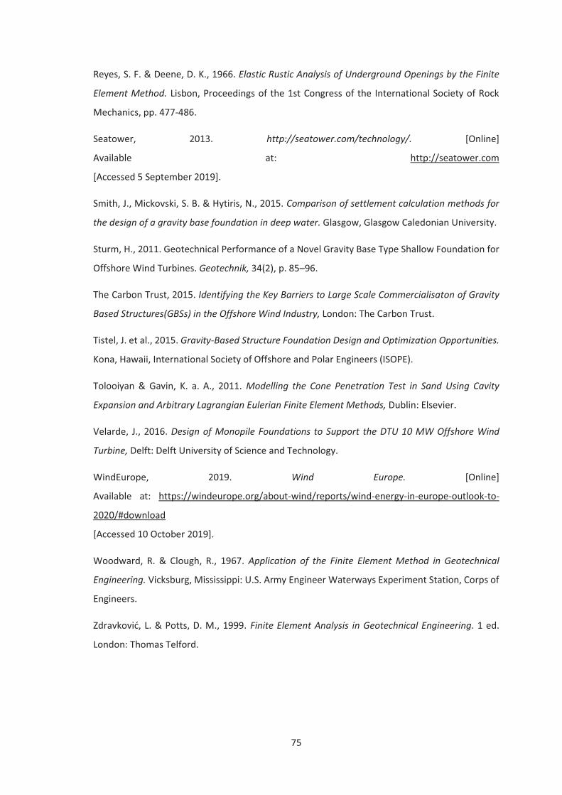
75

Reyes, S. F. & Deene, D. K., 1966. Elastic Rustic Analysis of Underground Openings by the Finite

Element Method. Lisbon, Proceedings of the 1st Congress of the International Society of Rock

Mechanics, pp. 477-486.

Seatower, 2013. http://seatower.com/technology/. [Online]

Available at: http://seatower.com

[Accessed 5 September 2019].

Smith, J., Mickovski, S. B. & Hytiris, N., 2015. Comparison of settlement calculation methods for

the design of a gravity base foundation in deep water. Glasgow, Glasgow Caledonian University.

Sturm, H., 2011. Geotechnical Performance of a Novel Gravity Base Type Shallow Foundation for

Offshore Wind Turbines. Geotechnik, 34(2), p. 85–96.

The Carbon Trust, 2015. Identifying the Key Barriers to Large Scale Commercialisaton of Gravity

Based Structures(GBSs) in the Offshore Wind Industry, London: The Carbon Trust.

Tistel, J. et al., 2015. Gravity-Based Structure Foundation Design and Optimization Opportunities.

Kona, Hawaii, International Society of Offshore and Polar Engineers (ISOPE).

Tolooiyan & Gavin, K. a. A., 2011. Modelling the Cone Penetration Test in Sand Using Cavity

Expansion and Arbitrary Lagrangian Eulerian Finite Element Methods, Dublin: Elsevier.

Velarde, J., 2016. Design of Monopile Foundations to Support the DTU 10 MW Offshore Wind

Turbine, Delft: Delft University of Science and Technology.

WindEurope, 2019. Wind Europe. [Online]

Available at: https://windeurope.org/about-wind/reports/wind-energy-in-europe-outlook-to-

2020/#download

[Accessed 10 October 2019].

Woodward, R. & Clough, R., 1967. Application of the Finite Element Method in Geotechnical

Engineering. Vicksburg, Mississippi: U.S. Army Engineer Waterways Experiment Station, Corps of

Engineers.

Zdravković, L. & Potts, D. M., 1999. Finite Element Analysis in Geotechnical Engineering. 1 ed.

London: Thomas Telford.

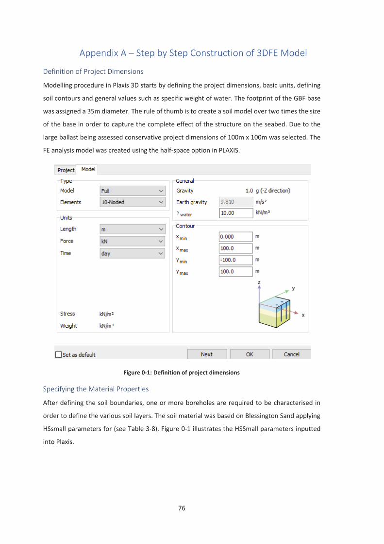
76

Appendix A – Step by Step Construction of 3DFE Model

Definition of Project Dimensions

Modelling procedure in Plaxis 3D starts by defining the project dimensions, basic units, defining

soil contours and general values such as specific weight of water. The footprint of the GBF base

was assigned a 35m diameter. The rule of thumb is to create a soil model over two times the size

of the base in order to capture the complete effect of the structure on the seabed. Due to the

large ballast being assessed conservative project dimensions of 100m x 100m was selected. The

FE analysis model was created using the half-space option in PLAXIS.

Figure 0-1: Definition of project dimensions

Specifying the Material Properties

After defining the soil boundaries, one or more boreholes are required to be characterised in

order to define the various soil layers. The soil material was based on Blessington Sand applying

HSsmall parameters for (see Table 3-8). Figure 0-1 illustrates the HSSmall parameters inputted

into Plaxis.

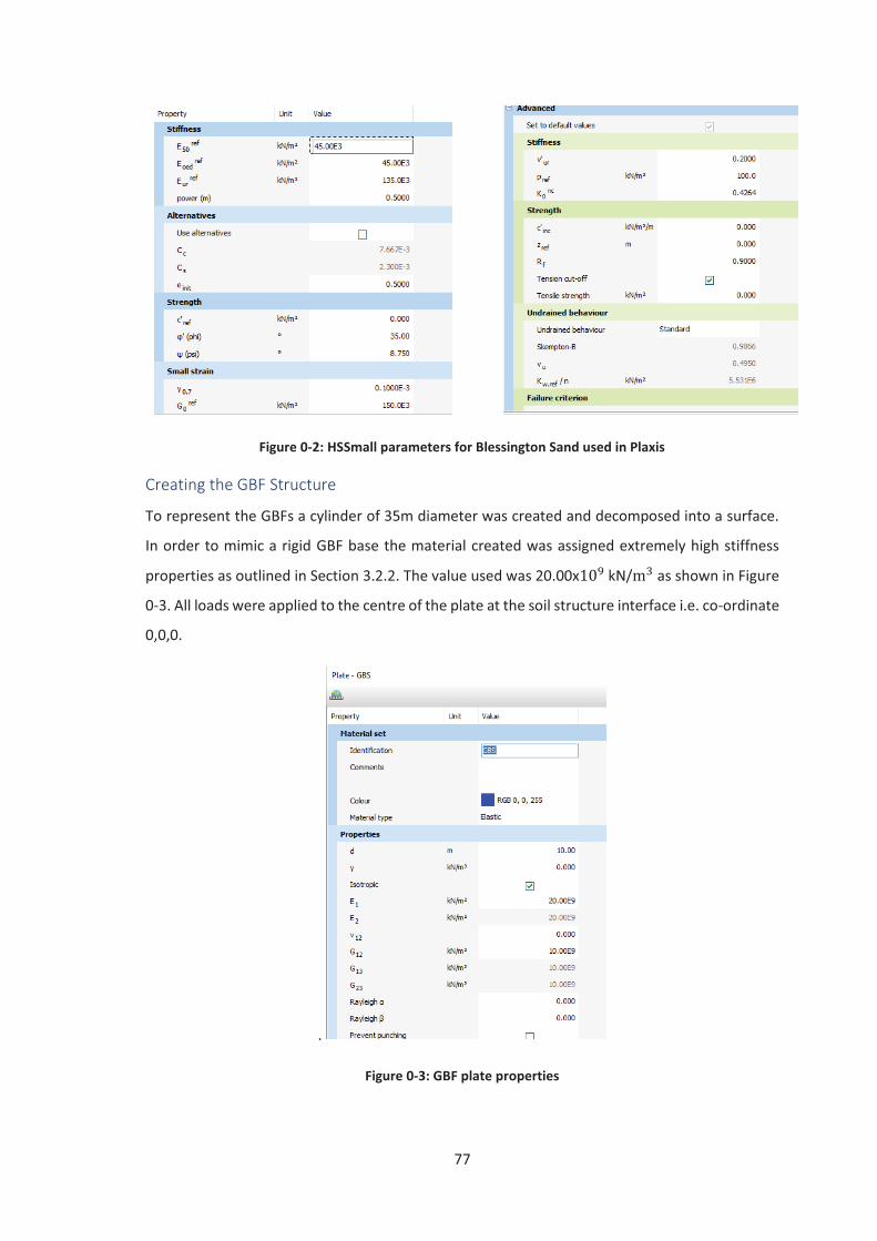
77

Figure 0-2: HSSmall parameters for Blessington Sand used in Plaxis

Creating the GBF Structure

To represent the GBFs a cylinder of 35m diameter was created and decomposed into a surface.

In order to mimic a rigid GBF base the material created was assigned extremely high stiffness

properties as outlined in Section 3.2.2. The value used was 20.00x kN/ as shown in Figure

0-3. All loads were applied to the centre of the plate at the soil structure interface i.e. co-ordinate

0,0,0.

.

Figure 0-3: GBF plate properties

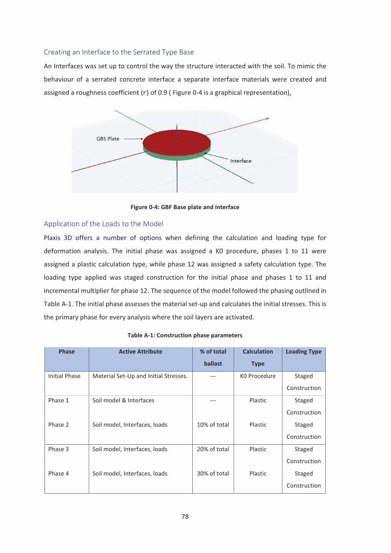
78

Creating an Interface to the Serrated Type Base

An Interfaces was set up to control the way the structure interacted with the soil. To mimic the

behaviour of a serrated concrete interface a separate interface materials were created and

assigned a roughness coefficient ( ) of 0.9 ( Figure 0-4 is a graphical representation),

Figure 0-4: GBF Base plate and interface

Application of the Loads to the Model

Plaxis 3D offers a number of options when defining the calculation and loading type for

deformation analysis. The initial phase was assigned a K0 procedure, phases 1 to 11 were

assigned a plastic calculation type, while phase 12 was assigned a safety calculation type. The

loading type applied was staged construction for the initial phase and phases 1 to 11 and

incremental multiplier for phase 12. The sequence of the model followed the phasing outlined in

Table A-1. The initial phase assesses the material set-up and calculates the initial stresses. This is

the primary phase for every analysis where the soil layers are activated.

Table A-1: Construction phase parameters

Phase Active Attribute % of total

ballast

Calculation

Type

Loading Type

Initial Phase Material Set-Up and Initial Stresses. --- K0 Procedure Staged

Construction

Phase 1 Soil model & Interfaces --- Plastic Staged

Construction

Phase 2 Soil model, Interfaces, loads 10% of total Plastic Staged

Construction

Phase 3 Soil model, Interfaces, loads 20% of total Plastic Staged

Construction

Phase 4 Soil model, Interfaces, loads 30% of total Plastic Staged

Construction

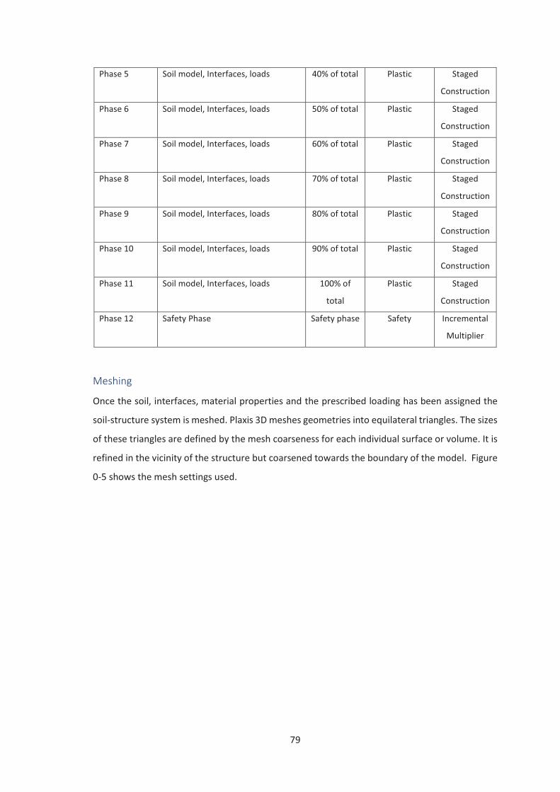
79

Phase 5 Soil model, Interfaces, loads 40% of total Plastic Staged

Construction

Phase 6 Soil model, Interfaces, loads 50% of total Plastic Staged

Construction

Phase 7 Soil model, Interfaces, loads 60% of total Plastic Staged

Construction

Phase 8 Soil model, Interfaces, loads 70% of total Plastic Staged

Construction

Phase 9 Soil model, Interfaces, loads 80% of total Plastic Staged

Construction

Phase 10 Soil model, Interfaces, loads 90% of total Plastic Staged

Construction

Phase 11 Soil model, Interfaces, loads 100% of

total

Plastic Staged

Construction

Phase 12 Safety Phase Safety phase Safety Incremental

Multiplier

Meshing

Once the soil, interfaces, material properties and the prescribed loading has been assigned the

soil-structure system is meshed. Plaxis 3D meshes geometries into equilateral triangles. The sizes

of these triangles are defined by the mesh coarseness for each individual surface or volume. It is

refined in the vicinity of the structure but coarsened towards the boundary of the model. Figure

0-5 shows the mesh settings used.

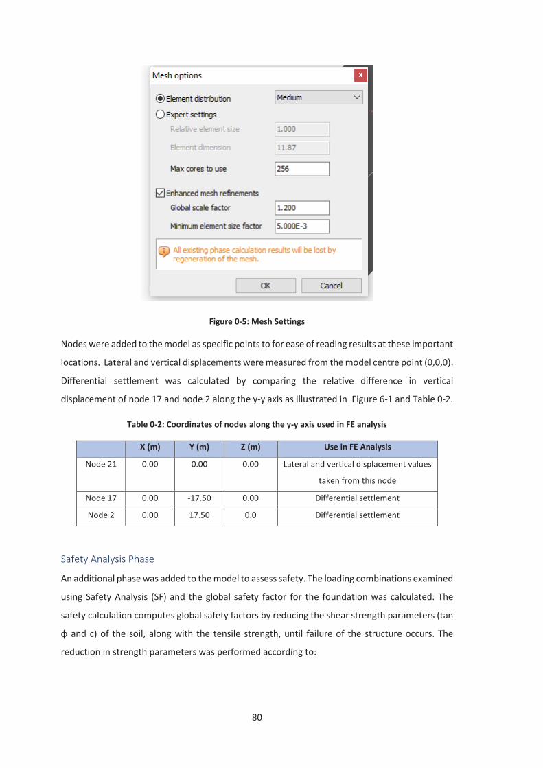
80

Figure 0-5: Mesh Settings

Nodes were added to the model as specific points to for ease of reading results at these important

locations. Lateral and vertical displacements were measured from the model centre point (0,0,0).

Differential settlement was calculated by comparing the relative difference in vertical

displacement of node 17 and node 2 along the y-y axis as illustrated in Figure 6-1 and Table 0-2.

Table 0-2: Coordinates of nodes along the y-y axis used in FE analysis

X (m) Y (m) Z (m) Use in FE Analysis

Node 21 0.00 0.00 0.00 Lateral and vertical displacement values

taken from this node

Node 17 0.00 -17.50 0.00 Differential settlement

Node 2 0.00 17.50 0.0 Differential settlement

Safety Analysis Phase

An additional phase was added to the model to assess safety. The loading combinations examined

using Safety Analysis (SF) and the global safety factor for the foundation was calculated. The

safety calculation computes global safety factors by reducing the shear strength parameters (tan

φ and c) of the soil, along with the tensile strength, until failure of the structure occurs. The

reduction in strength parameters was performed according to:

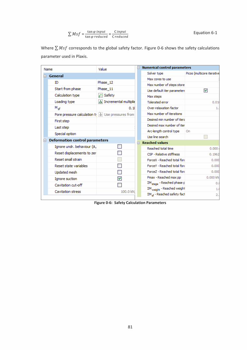
81

= = Equation 6-1

Where corresponds to the global safety factor. Figure 0-6 shows the safety calculations

parameter used in Plaxis.

Figure 0-6: Safety Calculation Parameters

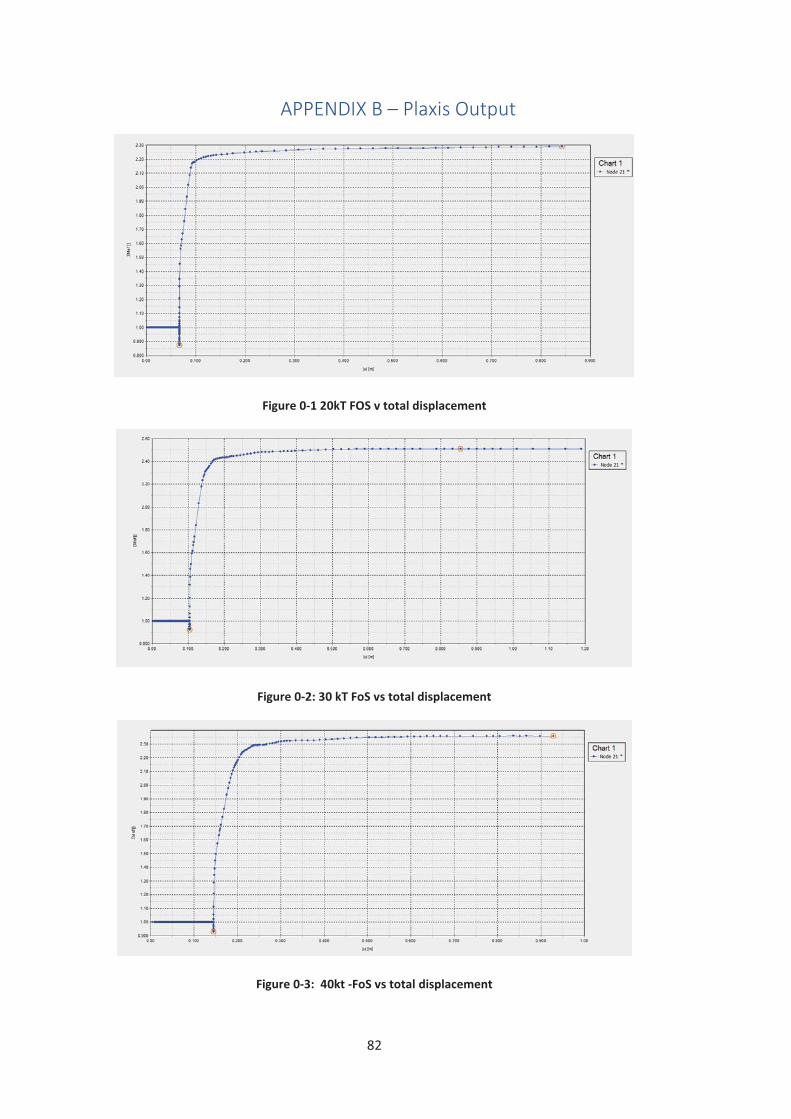
82

APPENDIX B – Plaxis Output

Figure 0-1 20kT FOS v total displacement

Figure 0-2: 30 kT FoS vs total displacement

Figure 0-3: 40kt -FoS vs total displacement

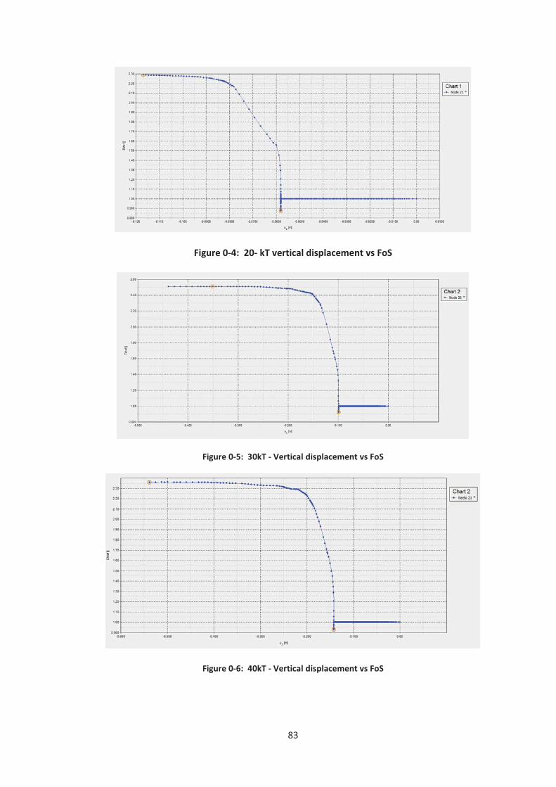
83

Figure 0-4: 20- kT vertical displacement vs FoS

Figure 0-5: 30kT - Vertical displacement vs FoS

Figure 0-6: 40kT - Vertical displacement vs FoS

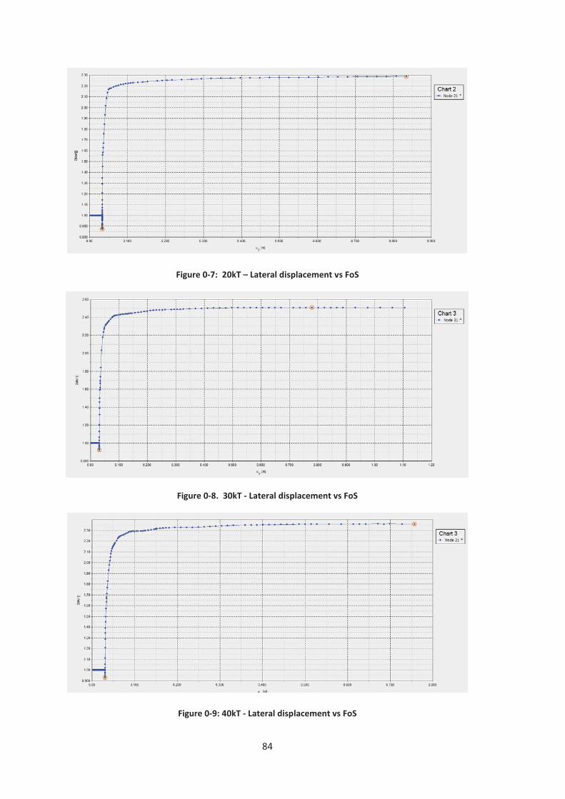
84

Figure 0-7: 20kT – Lateral displacement vs FoS

Figure 0-8. 30kT - Lateral displacement vs FoS

Figure 0-9: 40kT - Lateral displacement vs FoS