Embed Size (px)
Citation preview
1. Introduction
A job shop is a multi-stage production system. Each job needs to undergo several operations to become
a finished product. In a job shop, only a single machine is capable of processing each operation. This
one-to-one relationship will cause blocking of production when any machine breaks down. To reduce
the risk of blocking, a flexible job shop forms a group of capable machines for each operation. The term
‘‘flexible’’ comes from the flexibility of routing jobs. If each machine is capable of processing all
operations, the shop is very flexible, otherwise, it is partially flexible. Once the machine shop is properly
capacitated with the proper number of machines, then two main trends have proven effective in
improving the performance of the job shop or flexible job shop: Scheduling and cellular manufacturing.
Scheduling is always one of the keys to the success of a production system. Properly utilizing the
resources increases machine utilization, reduces work-in-process (WIP) level, shortens time to market,
and meets customers’ demands [30]. However, scheduling is a continuous challenge but it must be
preceded with equipment arrangement through cellular manufacturing. Cellular manufacturing is used
Corresponding author
E-mail: [email protected]
DOI: 10.22105/jarie.2017.54711
Design of Manufacturing Cells Pharmaceutical Factory
Mahmoud. A. Barghash1, Nabeel Al-Mandahawi 2, N. AbuJbara2, R. Al-
Abbadi2, S. Hussein2
1Department of Industrial Engineering, University of Jordan Amman 11942, Jordan. 2Department of Industrial Engineering, Hashemite University Zarqa, Jordan.
A B S T R A C T P A P E R I N F O
Cellular manufacturing is an important tool for manufacturing firms which leads to
better productivity, focused and specialized manufacturing process. To utilize this
important tool, the machines have to be grouped into cells. This work is related to using
cellular manufacturing in a pharmaceutical factory with alternative routing. This adds
more choices in the decision making process and presses for a better tool to make
optimal selection. Several objectives may be considered to improve the productivity
objectives such as the total number of exits and planning and scheduling robustness
related objectives like bottleneck utilization and load balance between and within the
alternative routes. Analytical hierarchical process (AHP) is used as a multi-objective
decision making process to evaluate the best scenario amongst generated using
simulation as a tool for modeling and evaluating the output for each scenario. Three
customer case studies were considered with different preferences and the AHP
evaluated the best scenario to fit these preferences. The best scenario can vary from
one customer preferences to another but for the current system it turned out to be the
same choice.
Chronicle:
Received: 26 June 2017
Accepted: 12 September 2017
Keywords : Cellular Manufacturing .
Analytical Hierarchical
Process. Simulation.
Multi-objective Analysis .
J. Appl. Res. Ind. Eng. Vol. 4, No. 3 (2017)158–173
Journal of Applied Research on Industrial
Engineering
www.journal-aprie.com
159 Design of manufacturing cells pharmaceutical factory
to overcome the deficiencies of job shop manufacturing, including excessive setup times and high level
of in-process inventories. In cellular manufacturing, part-families are identified and machine cells are
formed such that one or more part-families can be fully processed within a single machine cell [27].
Cellular manufacturing systems have shown encouraging results in batch manufacturing environments.
Significant improvements can be achieved by grouping machines into cells dedicated to processing a
sub-set of the total production. The advantages of cellular manufacturing include reduction in setup
times, reduction of material handling times, reduced WIP, increased machine and tool utilization and
improved operator utilization [20], throughput time reduction, smaller work in process inventories,
manufacturing flexibility increase, product quality improvement and production planning and control
simplification [26].
The benefits of cellular manufacturing organization can be strongly affected by the environment
uncertainty, such as that associated with resource dependability and demand variability [21, 22].
Flexibility is usually considered in the design and operation of a cellular manufacturing system (CMS)
to reduce the risks associated with uncertainty [23, 24]. Among the several types of flexibility, routing
flexibility, the ability to use alternative routes inside a cell, or the ability to route parts to cells offering
the same processes can strongly affect CMS performance [25]. In environments characterized by low
resource dependability, the benefits of routing flexibility can balance the costs of material handling,
fixtures, increased set-up times, etc. Therefore, a trade-off between productivity and flexibility can then
be searched.
Generally, a cellular manufacturing system is usually designed based on a single machine-part matrix.
When the product mix changes, the structure of the machine-part matrix representing the manufacturing
system changes too [28]. The performance of the system should be carefully evaluated to address the
important objectives relevant to the manufacturing process to avoid creating bottleneck machines,
which would deteriorate the schedule quality; on the other hand, one should aim at minimizing costs.
Assessing the tradeoff between these possibly conflicting objectives is difficult; actually, it is a multi-
objective problem with respect to the load balancing and cost objectives [30]. Many approaches
proposed to date base their cell formation on similarity coefficients among the parts. These coefficients
can be generated using a coding system [1]. Other methods used to generate similarity measures include
the Jaccards similarity coefficient method, a weighted similarity measure [2], process based similarity
coefficients [3] and similarity coefficients based on part loading [4]. A different approach towards
cellular design is part clustering using the production flow analysis (PFA) which uses a matrix
representing the relations among the parts and the machines. The matrix, which is usually binary, is
termed component incidence matrix. Many matrix-based methods have been proposed for the cell
formation design. Examples are the Rank-Order method [5], the extended Rank-Order method [6],
MODROC [7], and a progressive restructuring method [8]. Another approach for clustering is the
hierarchical clustering approach, which uses methods such as single linkage clustering [2, 9, 10] and
average linkage [11]. Part grouping methods also include optimization techniques such as linear
programming [12], integer programming [13], and dynamic programming [4]. A multi-objective cluster
analysis was proposed in [14]. Newer methods for clustering use Fuzzy Sets [15], and Neural Network
[16]. A good set of introductory references to distributed problem solving can be found in [17-19].
Alternative routing and replicate machine is considered as a flexibility factor that adds to the robustness
against uncertainty and has been addressed [32, 33] along with the intercell movement objective [31,
31] or by adding a flexibility objective [31, 32, 34, 35], costs of intercell movements between machine
operations and machine investment[31, 37].
Barghash et al. / J. Appl. Res. Ind. Eng. 4(3) (2017) 158-173 160
Moreover, the Analytic Hierarchy Process (AHP) is a decision analysis technique used to evaluate
complex multi-attributed alternatives with conflicting objectives among one or more actors. The process
involves hierarchical decomposition of the overall evaluation problem into sub problems that can be
easily comprehended and evaluated. The benefits of the AHP include its ability to handle multiple
stakeholders with multiple objectives, the inclusion of possible interaction effects and the relative ease
of computation. In addition, with the AHP there is no need to explicitly estimate a utility function since
the AHP deals with stated preferences at each step [42]. Several alternatives has been used such as
Pareto weighting technique or utility weighting for the evaluation of the multi-objective problem.
However, these techniques-although are successful in transforming the multi-objective into a single
objective might not capture the total relevant experience of the expert or might include subjective
mistakes. AHP includes multiple pairwise comparisons of the objectives and the alternatives against the
objectives with consistency check, which enables more accurate capturing of the experience and
produces a more accurate weighting of the factors. Furthermore, for the cases of complex,
manufacturing processes, simulation had been used to model and evaluate the single objective problem
or the multi-objective cellular design problem [31, 38, 39, 40, 41]. Simulation is not a cellular
manufacturing algorithm, but is a scenario evaluation one. When compared to a scheduler, mathematical
model, queuing, Petri net or any other stochastic technique, simulation proves to be the most flexible
and accurate modeling technique.
In this work, we have tackled a real case study of cellular manufacturing design in a pharmaceutical
factory with all its added complexity of machine set-up time and failure, employee shifts and the
alternative routing. This type of complexity makes discrete event simulation the most logical choice for
system modeling. We have also addressed the problem as a multi-objective with load balance and
productivity in mind and selective a more consistent group of objective functions to reflect load
imbalance. Number of scenarios has been generated and AHP was used to evaluate the performance for
each alternative.
2. AHP Basic Analysis
Different quality characteristics have diverse responses to the same change in input parameters.
Consequently, optimal point for all objectives cannot be achieved concurrently. Manufacturers must
then prioritize their objectives. AHP includes a pairwise comparison between each quality
measurements to give a specific weight for each objective quality characteristic. In relation to TED,
pairwise comparison is done between all experiments for each individual objective characteristic. This
in turn gives a weight for the level of achieving of the quality characteristic by each experiment. A
simple multiplication between the weight of the quality characteristic and the weight of the experiment
and a simple sum will give an overall weight for each process setting. The AHP then includes a
hierarchy composed of two main levels, objectives experiments comparison level. The AHP is a
systematic analysis technique developed for multi-criteria decision. Its operating mode lays on the
decomposing and structuring of a complex issue into several levels, rigorous definition of manager
priorities, and computation of weights associated to the alternatives. The output of AHP is a ranking
indicating the overall preference for each decision alternative [12]. The development of the AHP model
is achieved in three steps [13]: Multi-quality optimization, hierarchical modeling, and evaluation.
The purpose of the AHP is to evaluate the overall achievement weight or score for each process setting
(experiment). This is achieved firstly through pairwise comparison between each two quality
characteristics and filling the comparison matrix A ( n n ) of the second level of the hierarchy, where
n is the number of quality characteristics or objectives. Subsequently, the relative weight for each
161 Design of manufacturing cells pharmaceutical factory
quality characteristic is calculated and a consistency index is calculated as given by the following
equations [14]:
*AAB (1)
n
i
jij
1
BC
(2)
.
iC
CWq
(3)
Where, Wqi is the weight of importance for objective quality characteristic i. Column sum vector is:
n
i
ijjE1
A
(4)
The Maximum Eigen value:
* max WqE
(5)
Consistency Index:
1
max
n
nCI
(6)
The main advantage of AHP lies with consistency check. Where the comparison is checked using the
CI index. Saaty [14] stated that for comparison to be consistent CI<0.10. The above described pairwise
comparison is repeatedly performed for all experiments for their performance with respect to each
quality characteristic. In this case, Weij is evaluated as the weight coefficient of the experiment j in
relation to quality characteristic i. The overall weight for each experimental setting is merely the sum
of the multiplication of the weight of experiment j in relation to experiment i and the coefficient of
quality characteristic i (See Eq. (7)).
.1
n
i
iijj WqWew (7)
Where, wj is AHP overall weight achieved by the jth experimental setting.
3. Methodology
This work is related to applying AHP and simulation to cell design in manufacturing for the case of
high flexibility and alternative routing. The basic steps for the suggested methodology are:
i. Objectives selection: The objectives should balance between the flexibility and productivity
measures.
ii. Pairwise analysis for the objectives to determine the relative weight for each objective.
iii. Scenario generation: Where the possible scenarios are generated based on acceptable changes
for the system.
iv. Objectives evaluation for alternative cell design scenarios using simulation.
v. Pairwise comparison for the alternative cell design scenarios against each objective function
to evaluate the relative weight.
vi. Evaluating the final performance measure for each scenario.
Barghash et al. / J. Appl. Res. Ind. Eng. 4(3) (2017) 158-173 162
3.1 Objective Suggestion
Huge emphasis in scheduling and optimization is placed on productivity measures. However, the
optimal solution might not be robust enough to face changes in the process, such as machine failure.
Therefore, alternative objective function should be considered such as operation cost and/or total exist
to consider cases when the bottleneck machine may fail, since the probability of failure increases
appreciably with high utilization. A further complication arises if we consider a truly multi-objective
approach since assessing the tradeoff between schedule quality and costs is not easy [29]. The
traditional scheduling problem lists schedule based objectives such as average flow time, global
earliness, lateness, production rate etc. However, these objectives may not be the proper ones to select
for balancing the load on different machines. Alternative objectives has been used for cell design such
as work in process, intercell movement, total investment. Even these cellular manufacturing objectives
may not fit to all case. For example, the work in process inventory (WIP) objective may not fit
applications where the pull system is applied. That is a case where the WIP is controlled through a
strict pull system. In addition, the investment costs is not applicable to the case when the factory is only
rearranging and no new cost are incurred. If each product passes through the same routing as the other,
then the intercell movement is a reflection of the number of products produced (total exits in simulation
terminology) and is not an independent objective.
Therefore, for successful application of the AHP and the optimization process, the objectives must be
selected intelligently. For the problem on hand, the most important objective is the number of products
produced in a certain period of time (total number of exits in Promodel terms). This objective is tied to
the economics and feasibility of any decision to be made. However, this objective is not conclusive
since it does not reflect the balance of the schedule, which is tied to the robustness of the planning and
the scheduling process. For this purpose another set of objectives have been included which are related
to the machine utilization and delay process. These important objectives reflect machine utilization and
planning process robustness. Since already, the load is highly balanced and the process is uniform. We
also selected WIP and the average minutes in system. As a summary, in this research, a set of objective
functions have been selected which combine between the workstation balance and work in process
inventory, these objectives are summarized as below:
i. Objective A: load imbalance 1: load imbalance within cell reflected by the difference in
utilization between the maximum utilization difference and the minimum utilization
difference.
ii. Objective B: Total exit.
iii. Objective C: load imbalance 2: Load imbalance between cells reflected by the difference in
utilization between the bottlenecks of each cell.
iv. Objective D: Work In Process (WIP).
v. Objective E: Average minute in the system.
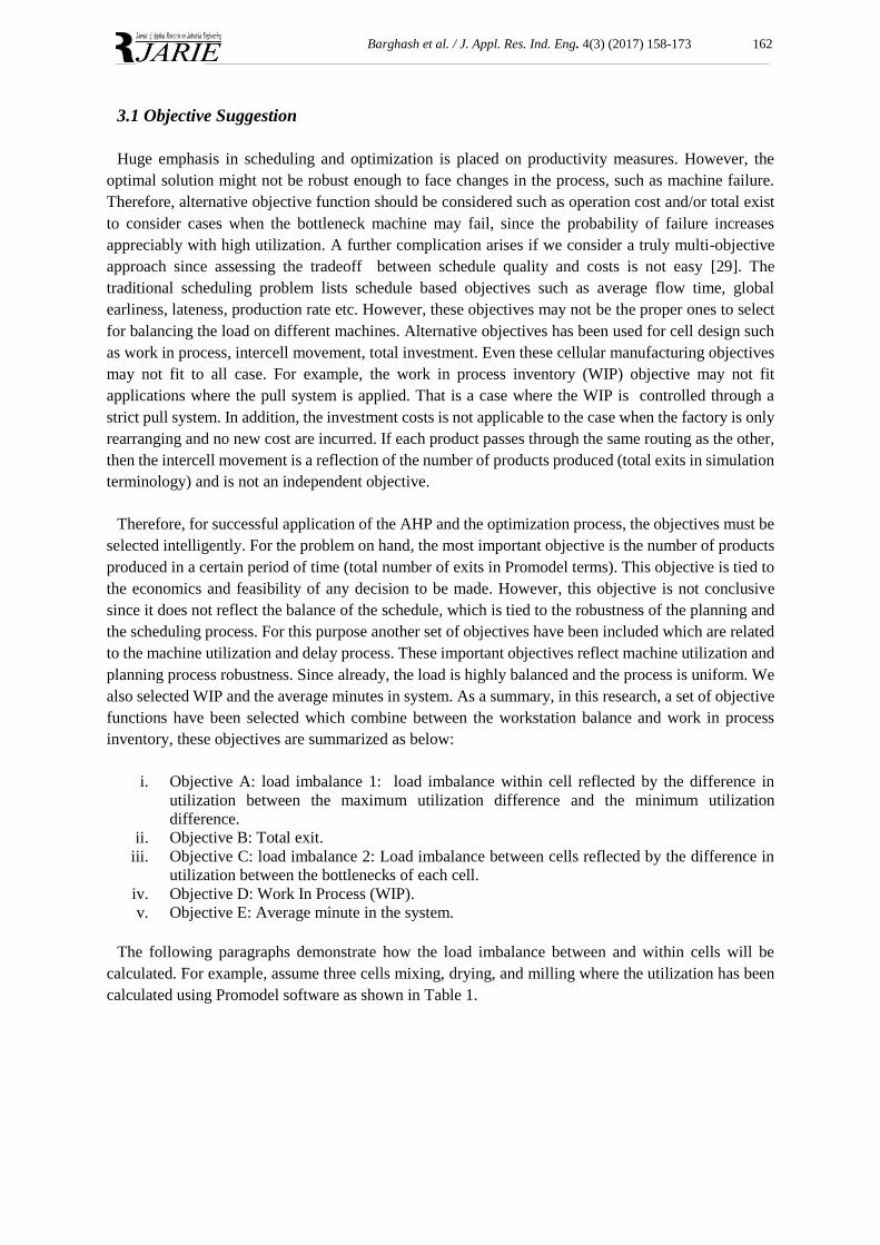
The following paragraphs demonstrate how the load imbalance between and within cells will be
calculated. For example, assume three cells mixing, drying, and milling where the utilization has been
calculated using Promodel software as shown in Table 1.
163 Design of manufacturing cells pharmaceutical factory
Table 1. Load imbalance 1 calculations.
Cell/ mlc Mixing% Drying% Milling% Max – Second utilization
Cell 1 30.26 25.79 34.57 4.31%
Cell 2 61.31 24.65 34.57 26.74%
Cell 3 65.94 62.34 23.40 3.6%
Cell 4 54.78 24.65 23.40 30.13%
Cell 5 49.44 19.12 23.91 25.53%
Load balance1= Max- Min 26.53%
The difference between the bottleneck machine utilization and the second in line represents a window
of opportunity for improvement. We can improve cell production by switching machines until little
difference between the two is noticed. Thus, this imbalance difference reflects the arrangement quality
of the machines. The difference between the Max difference and the minimum difference reflects this
arrangement quality. The first load imbalance is given by Eq. (8). For each cell and is shown in Table
1 column 5. The objective measure is the difference of the imbalance between the maximum and the
minimum imbalance. Ideally, this objective is zero that is there no difference within the cell between
the different machines. However, it can be zero if all the cells have the same imbalance that is the max
imbalance - min imbalance are equal which means that all arrangement are equal.
Load imbalance = within cell (max. utilization – Second utilization). (8)
For the current production line the total imbalance equals = 30.13 – 3.6 = 26.53.
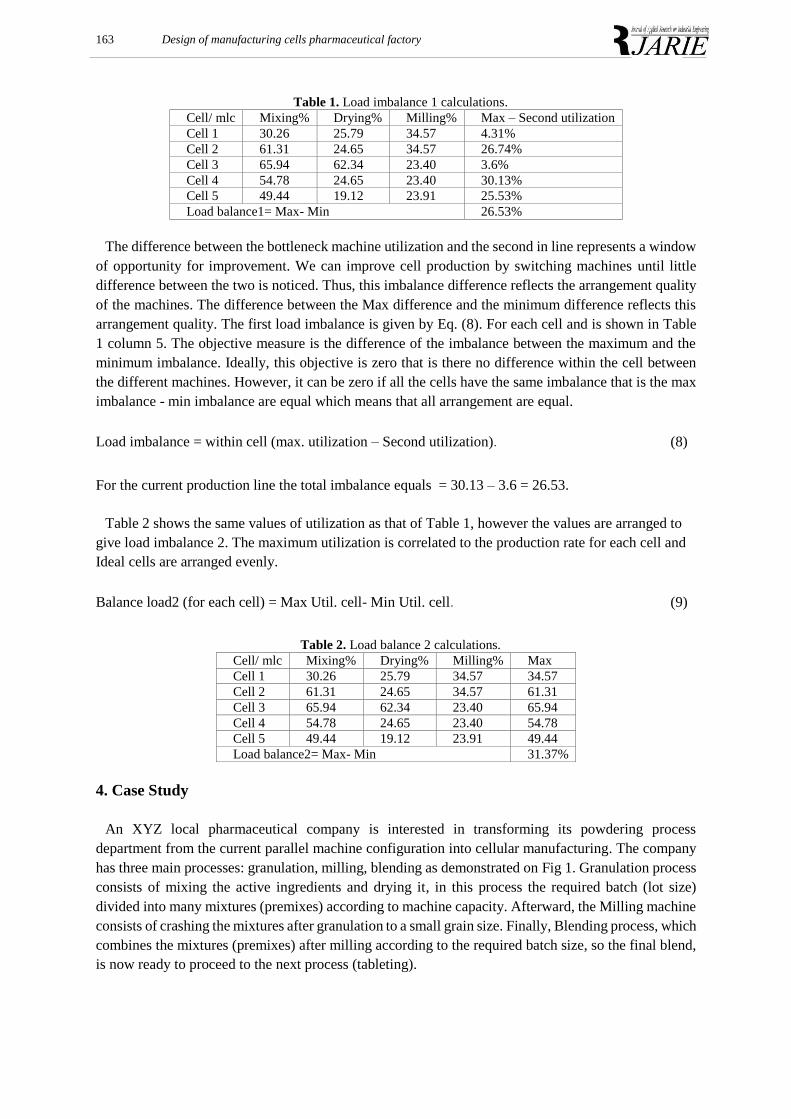
Table 2 shows the same values of utilization as that of Table 1, however the values are arranged to
give load imbalance 2. The maximum utilization is correlated to the production rate for each cell and
Ideal cells are arranged evenly.
Balance load2 (for each cell) = Max Util. cell- Min Util. cell. (9)
Table 2. Load balance 2 calculations.
Cell/ mlc Mixing% Drying% Milling% Max
Cell 1 30.26 25.79 34.57 34.57
Cell 2 61.31 24.65 34.57 61.31
Cell 3 65.94 62.34 23.40 65.94
Cell 4 54.78 24.65 23.40 54.78
Cell 5 49.44 19.12 23.91 49.44
Load balance2= Max- Min 31.37%
4. Case Study
An XYZ local pharmaceutical company is interested in transforming its powdering process
department from the current parallel machine configuration into cellular manufacturing. The company
has three main processes: granulation, milling, blending as demonstrated on Fig 1. Granulation process
consists of mixing the active ingredients and drying it, in this process the required batch (lot size)
divided into many mixtures (premixes) according to machine capacity. Afterward, the Milling machine
consists of crashing the mixtures after granulation to a small grain size. Finally, Blending process, which
combines the mixtures (premixes) after milling according to the required batch size, so the final blend,
is now ready to proceed to the next process (tableting).
Barghash et al. / J. Appl. Res. Ind. Eng. 4(3) (2017) 158-173 164
Granulation
(Mixing & drying)Milling Blending
Fig 1. Basic processing steps in the powdering department.
Furthermore, in the XYZ pharmaceutical company each machine consists of different types as shown
in Table 2, where variability exists due to difference from the manufacturer source. The name given to
each machine is the same name known by the workers and recorded in the factory records.
Table 3. List of the machines in the XYZ company. Mixing machine Drying machine Milling machine
Mixer E Aeromatic C Fitz mill Mixer L-150 A Aeromatic A Oscillator
Mixer L-150 B Oven Glatt cone mill
Mixer H Glatt dryer
Glatt mixer
In a usual manufacturing process, machine is not available 100% of the time. It is customary to have
set-up time and machine failures. This add's up to the complexity of the cellular manufacturing
processes and if these are significant, then simple models might not be suffice. The powder machine’s
is subjected to the following setup and failure types:
i. Dry cleaning: A type of cleaning that is made to the machine after each premix of the same
product.
ii. Wet cleaning: A type of cleaning that is made to the machine when the concentration of the
same product changes.
iii. Full cleaning: A type of cleaning that is made between different products.
iv. Repair: An operation that fixes the machine when a malfunction occurs.
v. Preventive maintenance: Periodic maintenance (every 3 months) to check the machine state.
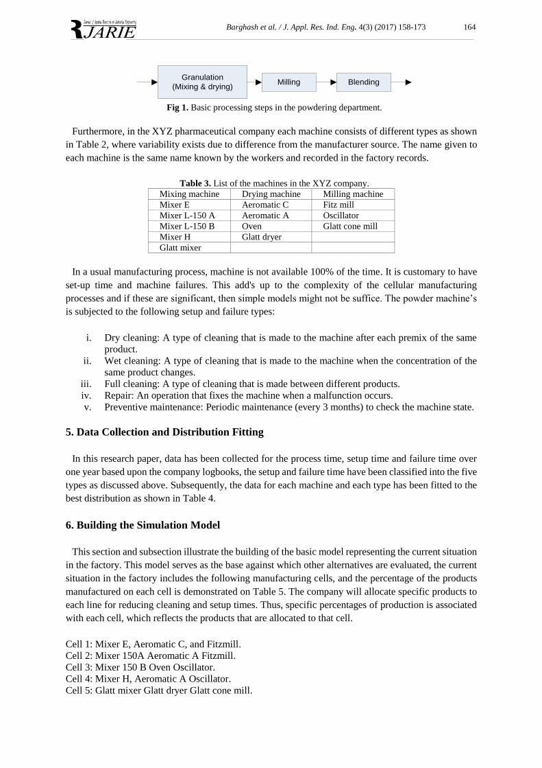
5. Data Collection and Distribution Fitting
In this research paper, data has been collected for the process time, setup time and failure time over
one year based upon the company logbooks, the setup and failure time have been classified into the five
types as discussed above. Subsequently, the data for each machine and each type has been fitted to the
best distribution as shown in Table 4.
6. Building the Simulation Model
This section and subsection illustrate the building of the basic model representing the current situation
in the factory. This model serves as the base against which other alternatives are evaluated, the current
situation in the factory includes the following manufacturing cells, and the percentage of the products
manufactured on each cell is demonstrated on Table 5. The company will allocate specific products to
each line for reducing cleaning and setup times. Thus, specific percentages of production is associated
with each cell, which reflects the products that are allocated to that cell.
Cell 1: Mixer E, Aeromatic C, and Fitzmill.
Cell 2: Mixer 150A Aeromatic A Fitzmill.
Cell 3: Mixer 150 B Oven Oscillator.
Cell 4: Mixer H, Aeromatic A Oscillator.
Cell 5: Glatt mixer Glatt dryer Glatt cone mill.
165 Design of manufacturing cells pharmaceutical factory
Table 4. A sample of the distribution fitted for the cleaning process and the repair.
Table 5. The percentage of products manufactured on each cell.
Cycle Total # of premix Percentage (%)
1 607 25.92 %
2 545 23.27 %
3 312 13.32 %
4 545 23.27 %
5 333 14.22 %
Sum 2342 100%
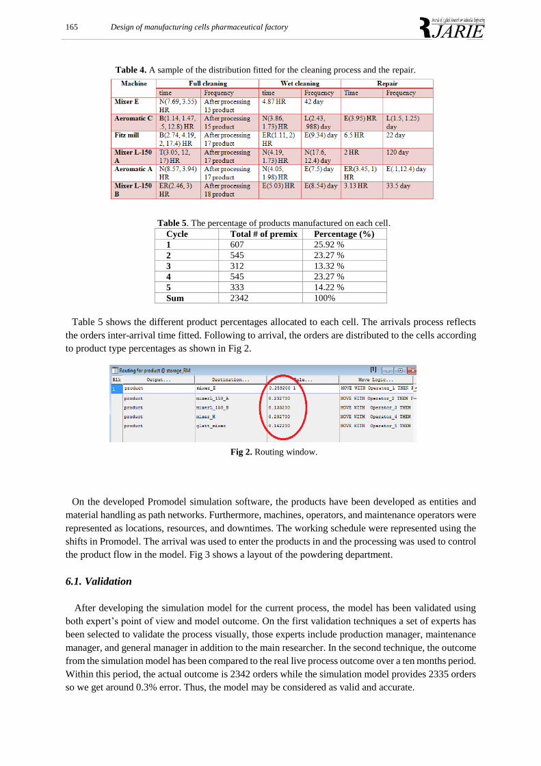
Table 5 shows the different product percentages allocated to each cell. The arrivals process reflects
the orders inter-arrival time fitted. Following to arrival, the orders are distributed to the cells according
to product type percentages as shown in Fig 2.
Fig 2. Routing window.
On the developed Promodel simulation software, the products have been developed as entities and
material handling as path networks. Furthermore, machines, operators, and maintenance operators were
represented as locations, resources, and downtimes. The working schedule were represented using the
shifts in Promodel. The arrival was used to enter the products in and the processing was used to control
the product flow in the model. Fig 3 shows a layout of the powdering department.
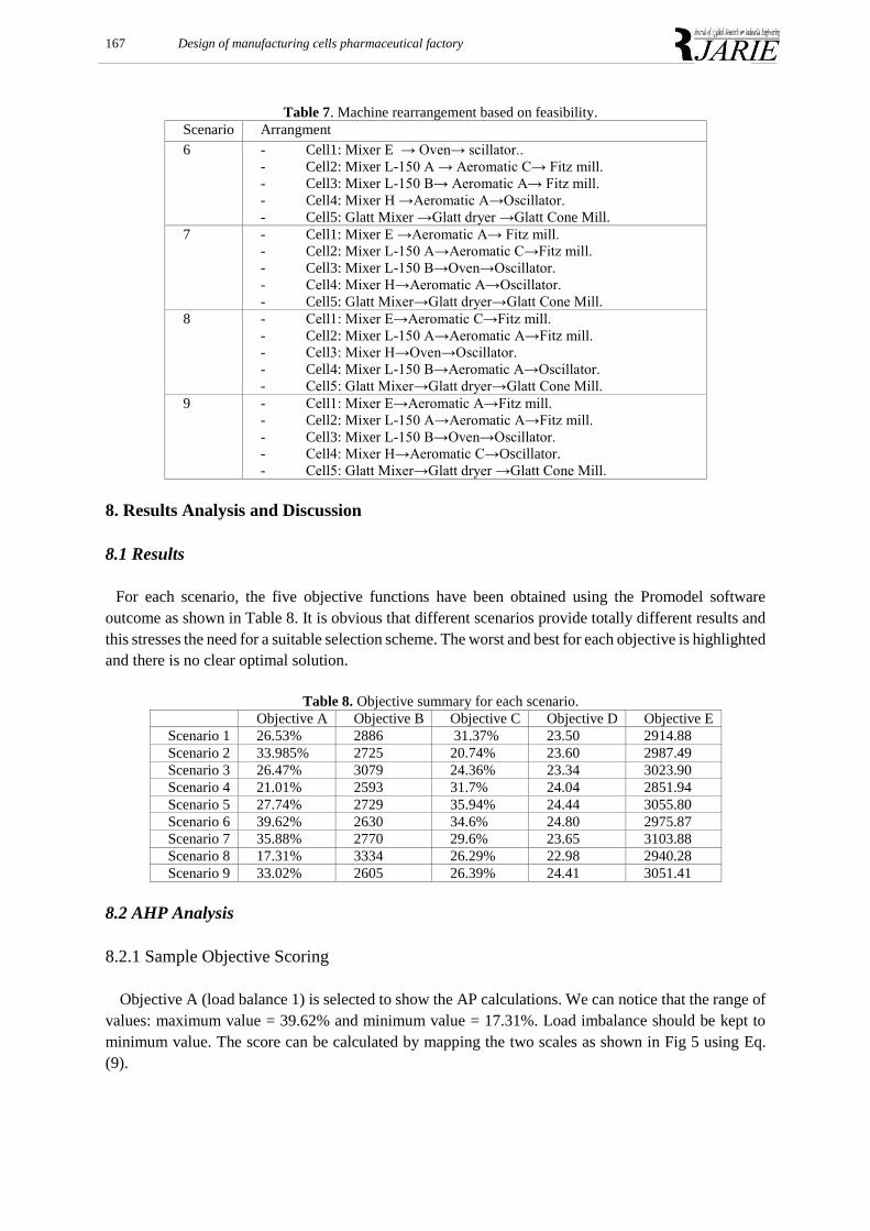
6.1. Validation
After developing the simulation model for the current process, the model has been validated using
both expert’s point of view and model outcome. On the first validation techniques a set of experts has
been selected to validate the process visually, those experts include production manager, maintenance
manager, and general manager in addition to the main researcher. In the second technique, the outcome
from the simulation model has been compared to the real live process outcome over a ten months period.
Within this period, the actual outcome is 2342 orders while the simulation model provides 2335 orders
so we get around 0.3% error. Thus, the model may be considered as valid and accurate.
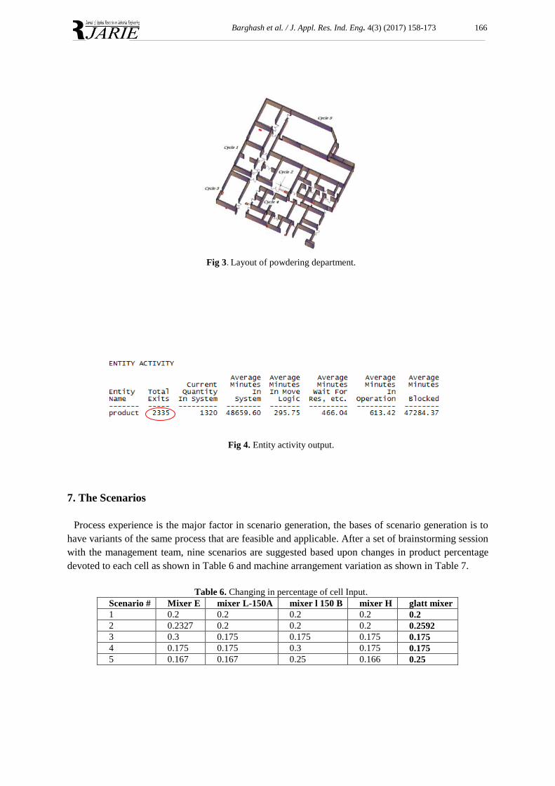
Barghash et al. / J. Appl. Res. Ind. Eng. 4(3) (2017) 158-173 166
Fig 3. Layout of powdering department.
Fig 4. Entity activity output.
7. The Scenarios
Process experience is the major factor in scenario generation, the bases of scenario generation is to
have variants of the same process that are feasible and applicable. After a set of brainstorming session
with the management team, nine scenarios are suggested based upon changes in product percentage
devoted to each cell as shown in Table 6 and machine arrangement variation as shown in Table 7.
Table 6. Changing in percentage of cell Input.
glatt mixer mixer H mixer l 150 B mixer L-150A Mixer E Scenario #
0.2 0.2 0.2 0.2 0.2 1
0.2592 0.2 0.2 0.2 0.2327 2
0.175 0.175 0.175 0.175 0.3 3
0.175 0.175 0.3 0.175 0.175 4
0.25 0.166 0.25 0.167 0.167 5
167 Design of manufacturing cells pharmaceutical factory
Table 7. Machine rearrangement based on feasibility.
Scenario Arrangment
6 - Cell1: Mixer E → Oven→ scillator..
- Cell2: Mixer L-150 A → Aeromatic C→ Fitz mill.
- Cell3: Mixer L-150 B→ Aeromatic A→ Fitz mill.
- Cell4: Mixer H →Aeromatic A→Oscillator.
- Cell5: Glatt Mixer →Glatt dryer →Glatt Cone Mill.
7 - Cell1: Mixer E →Aeromatic A→ Fitz mill.
- Cell2: Mixer L-150 A→Aeromatic C→Fitz mill.
- Cell3: Mixer L-150 B→Oven→Oscillator.
- Cell4: Mixer H→Aeromatic A→Oscillator.
- Cell5: Glatt Mixer→Glatt dryer→Glatt Cone Mill.
8 - Cell1: Mixer E→Aeromatic C→Fitz mill.
- Cell2: Mixer L-150 A→Aeromatic A→Fitz mill.
- Cell3: Mixer H→Oven→Oscillator.
- Cell4: Mixer L-150 B→Aeromatic A→Oscillator.
- Cell5: Glatt Mixer→Glatt dryer→Glatt Cone Mill.
9 - Cell1: Mixer E→Aeromatic A→Fitz mill.
- Cell2: Mixer L-150 A→Aeromatic A→Fitz mill.
- Cell3: Mixer L-150 B→Oven→Oscillator.
- Cell4: Mixer H→Aeromatic C→Oscillator.
- Cell5: Glatt Mixer→Glatt dryer →Glatt Cone Mill.
8. Results Analysis and Discussion
8.1 Results
For each scenario, the five objective functions have been obtained using the Promodel software
outcome as shown in Table 8. It is obvious that different scenarios provide totally different results and
this stresses the need for a suitable selection scheme. The worst and best for each objective is highlighted
and there is no clear optimal solution.
Table 8. Objective summary for each scenario.
Objective A Objective B Objective C Objective D Objective E
Scenario 1 26.53% 2886 31.37% 23.50 2914.88
Scenario 2 33.985% 2725 20.74% 23.60 2987.49
Scenario 3 26.47% 3079 24.36% 23.34 3023.90
Scenario 4 21.01% 2593 31.7% 24.04 2851.94
Scenario 5 27.74% 2729 35.94% 24.44 3055.80
Scenario 6 39.62% 2630 34.6% 24.80 2975.87
Scenario 7 35.88% 2770 29.6% 23.65 3103.88
Scenario 8 17.31% 3334 26.29% 22.98 2940.28
Scenario 9 33.02% 2605 26.39% 24.41 3051.41
8.2 AHP Analysis
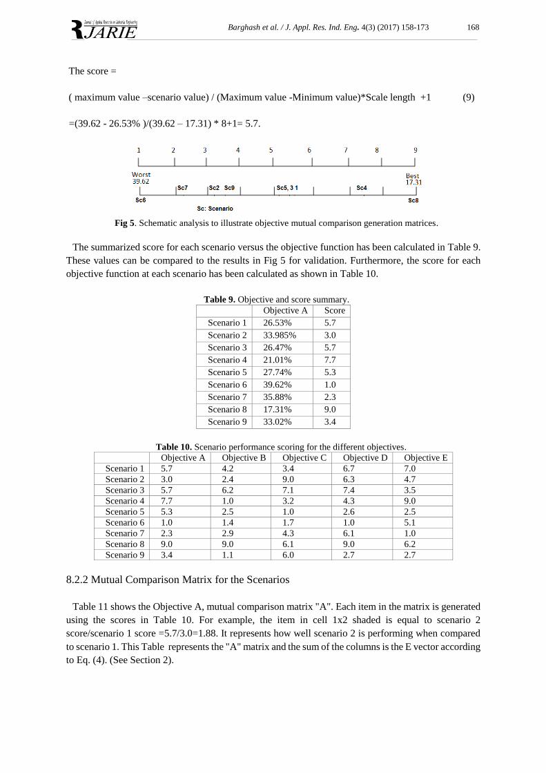
8.2.1 Sample Objective Scoring
Objective A (load balance 1) is selected to show the AP calculations. We can notice that the range of
values: maximum value = 39.62% and minimum value = 17.31%. Load imbalance should be kept to
minimum value. The score can be calculated by mapping the two scales as shown in Fig 5 using Eq.
(9).
Barghash et al. / J. Appl. Res. Ind. Eng. 4(3) (2017) 158-173 168
The score =
( maximum value –scenario value) / (Maximum value -Minimum value)*Scale length +1 (9)
=(39.62 - 26.53% )/(39.62 – 17.31) * 8+1= 5.7.
Fig 5. Schematic analysis to illustrate objective mutual comparison generation matrices.
The summarized score for each scenario versus the objective function has been calculated in Table 9.
These values can be compared to the results in Fig 5 for validation. Furthermore, the score for each
objective function at each scenario has been calculated as shown in Table 10.
Table 9. Objective and score summary.
Objective A Score
Scenario 1 26.53% 5.7
Scenario 2 33.985% 3.0
Scenario 3 26.47% 5.7
Scenario 4 21.01% 7.7
Scenario 5 27.74% 5.3
Scenario 6 39.62% 1.0
Scenario 7 35.88% 2.3
Scenario 8 17.31% 9.0
Scenario 9 33.02% 3.4
Table 10. Scenario performance scoring for the different objectives.
Objective A Objective B Objective C Objective D Objective E
Scenario 1 5.7 4.2 3.4 6.7 7.0
Scenario 2 3.0 2.4 9.0 6.3 4.7
Scenario 3 5.7 6.2 7.1 7.4 3.5
Scenario 4 7.7 1.0 3.2 4.3 9.0
Scenario 5 5.3 2.5 1.0 2.6 2.5
Scenario 6 1.0 1.4 1.7 1.0 5.1
Scenario 7 2.3 2.9 4.3 6.1 1.0
Scenario 8 9.0 9.0 6.1 9.0 6.2
Scenario 9 3.4 1.1 6.0 2.7 2.7
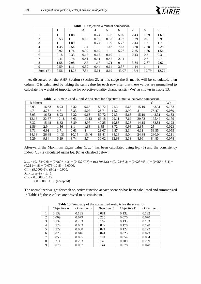
8.2.2 Mutual Comparison Matrix for the Scenarios
Table 11 shows the Objective A, mutual comparison matrix "A". Each item in the matrix is generated
using the scores in Table 10. For example, the item in cell 1x2 shaded is equal to scenario 2
score/scenario 1 score =5.7/3.0=1.88. It represents how well scenario 2 is performing when compared
to scenario 1. This Table represents the "A" matrix and the sum of the columns is the E vector according
to Eq. (4). (See Section 2).
169 Design of manufacturing cells pharmaceutical factory
Table 11. Objective a mutual comparison.
9 8 7 6 5 4 3 2 1 1.69 1.69 2.43 5.69 1.08 0.74 1 1.88 1 1 0.9 0.9 1.29 3.02 0.57 0.39 0.53 1 0.53 2 1.7 1.7 2.44 5.72 1.09 0.74 1 1.89 1 3 2.28 2.28 3.28 7.67 1.46 1 1.34 2.54 1.35 4 1.56 1.56 2.25 5.26 1 0.69 0.92 1.74 0.92 5 0.3 0.3 0.43 1 0.19 0.13 0.17 0.33 0.18 6 0.7 0.7 1 2.34 0.45 0.31 0.41 0.78 0.41 7 2.67 2.67 3.84 9 1.71 1.17 1.57 2.98 1.58 8 1 1 1.44 3.37 0.64 0.44 0.59 1.11 0.59 9 12.79 12.79 18.4 43.07 8.19 5.61 7.54 14.26 7.56 Sum (E)
As discussed on the AHP Section (Section 2), at this stage the B matrix will be calculated, then
column C is calculated by taking the sum value for each row after that these values are normalized to
calculate the weight of importance for objective quality characteristic (Wq) as shown in Table 13.
Table 12. B matrix and C and Wq vectors for objective a mutual pairwise comparison.
B Matrix C Wq
8.93 16.62 8.93 6.32 9.63 50.72 21.34 5.63 15.19 143.31 0.132
4.7 8.75 4.7 3.33 5.07 26.71 11.24 2.97 8 75.47 0.069
8.93 16.62 8.93 6.32 9.63 50.72 21.34 5.63 15.19 143.31 0.132
12.18 22.67 12.18 8.63 13.13 69.18 29.11 7.69 20.72 195.49 0.179
8.32 15.48 8.32 5.89 8.97 47.25 19.88 5.25 14.15 133.51 0.122
1.56 2.9 1.56 1.1 1.68 8.85 3.72 0.98 2.65 25 0.023
3.71 6.91 3.71 2.63 4 21.07 8.87 2.34 6.31 59.55 0.055
14.33 26.68 14.33 10.15 15.46 81.41 34.26 9.04 24.38 230.04 0.211
5.29 9.84 5.29 3.74 5.7 30.02 12.63 3.33 8.99 84.83 0.078
Afterward, the Maximum Eigen value (λmax ) has been calculated using Eq. (5) and the consistency
index (C.I) is calculated using Eq. (6) as clarified below:
λmax = (0.132*7.6) + (0.069*14.3) + (0.132*7.5) + (0.179*5.6) + (0.122*8.2) + (0.023*43.1) + (0.055*18.4) +
(0.211*4.8) + (0.078*12.8) = 9.0000.
C.I = (9.0000-9) / (9-1) = 0.000.
R.I (for n=9) = 1.45.
C.R = 0.00000/ 1.45
= 0.00000 < 0.1 (accepted).
The normalized weight for each objective function at each scenario has been calculated and summarized
in Table 13; these values are proved to be consistent.
Table 13. Summary of the normalized weights for the scenarios.
Objective E Objective D Objective C Objective B Objective A 0.132 0.132 0.081 0.135 0.132 1 0.070 0.070 0.215 0.079 0.069 2 0.133 0.133 0.169 0.203 0.132 3 0.178 0.178 0.077 0.033 0.179 4 0.122 0.122 0.024 0.080 0.122 5 0.023 0.023 0.041 0.046 0.023 6 0.054 0.054 0.104 0.095 0.055 7 0.209 0.209 0.145 0.293 0.211 8 0.078 0.078 0.144 0.037 0.078 9
Barghash et al. / J. Appl. Res. Ind. Eng. 4(3) (2017) 158-173 170
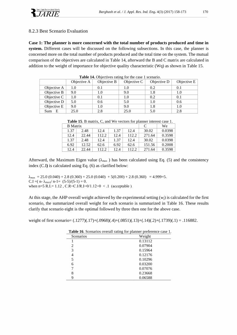
8.2.3 Best Scenario Evaluation
Case 1: The planner is more concerned with the total number of products produced and time in
system. Different cases will be discussed on the following subsections. In this case, the planner is
concerned more on the total number of products produced and the total time on the system. The mutual
comparison of the objectives are calculated in Table 14, afterward the B and C matrix are calculated in
addition to the weight of importance for objective quality characteristic (Wq) as shown in Table 15.
Table 14. Objectives rating for the case 1 scenario.
Objective E Objective D Objective C Objective B Objective A 0.1 0.2 1.0 0.1 1.0 Objective A 1.0 1.8 9.0 1.0 9.0 Objective B 0.1 0.2 1.0 0.1 1.0 Objective C 0.6 1.0 5.0 0.6 5.0 Objective D 1.0 1.8 9.0 1.0 9.0 Objective E 2.8 5.0 25.0 2.8 25.0 Sum E
Table 15. B matrix, C, and We vectors for planner interest case 1.
B Matrix C We
1.37 2.48 12.4 1.37 12.4 30.02 0.0398
12.4 22.44 112.2 12.4 112.2 271.64 0.3598
1.37 2.48 12.4 1.37 12.4 30.02 0.0398
6.92 12.52 62.6 6.92 62.6 151.56 0.2008
12.4 22.44 112.2 12.4 112.2 271.64 0.3598
Afterward, the Maximum Eigen value (λmax ) has been calculated using Eq. (5) and the consistency
index (C.I) is calculated using Eq. (6) as clarified below:
λmax = 25.0 (0.040) + 2.8 (0.360) + 25.0 (0.040) + 5(0.200) + 2.8 (0.360) = 4.999=5.
C.I =( n- λmax)/ n-1= (5-5)/(5-1) = 0.
when n=5 R.I.= 1.12 , C.R=C.I/R.I=0/1.12=0 < .1 (acceptable ).
At this stage, the AHP overall weight achieved by the experimental setting (wj) is calculated for the first
scenario, the summarized overall weight for each scenario is summarized in Table 16. These results
clarify that scenario eight is the optimal followed by three then one for the above case.
weight of first scenario= (.1277)(.17)+(.0968)(.4)+(.0851)(.13)+(.14)(.2)+(.1739)(.1) = .116882.
Table 16. Scenarios overall rating for planner preference case 1.
Scenarios Weight
1 0.13112
2 0.07904
3 0.15964
4 0.12176
5 0.10296
6 0.03200
7 0.07076
8 0.23668
9 0.06588
171 Design of manufacturing cells pharmaceutical factory
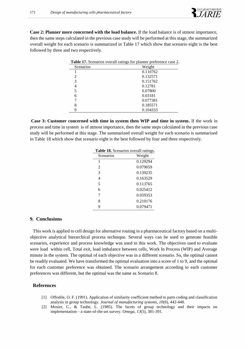
Case 2: Planner more concerned with the load balance. If the load balance is of utmost importance,
then the same steps calculated in the previous case study will be performed at this stage, the summarized
overall weight for each scenario is summarized in Table 17 which show that scenario eight is the best
followed by three and two respectively.
Table 17. Scenarios overall ratings for planner preference case 2.
Scenarios Weight
1 0.110762
2 0.132571
3 0.151762
4 0.12781
5 0.07800
6 0.03181
7 0.077381
8 0.185571
9 0.104333
Case 3: Customer concerned with time in system then WIP and time in system. If the work in
process and time in system is of utmost importance, then the same steps calculated in the previous case
study will be performed at this stage. The summarized overall weight for each scenario is summarized
in Table 18 which show that scenario eight is the best followed by four and three respectively.
Table 18. Scenarios overall ratings.
Scenarios Weight
1 0.129294
2 0.079059
3 0.139235
4 0.163529
5 0.113765
6 0.025412
7 0.059353
8 0.210176
9 0.079471
9. Conclusions
This work is applied to cell design for alternative routing in a pharmaceutical factory based on a multi-
objective analytical hierarchical process technique. Several ways can be used to generate feasible
scenarios, experience and process knowledge was used in this work. The objectives used to evaluate
were load within cell, Total exit, load imbalance between cells, Work In Process (WIP) and Average
minute in the system. The optimal of each objective was in a different scenario. So, the optimal cannot
be readily evaluated. We have transformed the optimal evaluation into a score of 1 to 9, and the optimal
for each customer preference was obtained. The scenario arrangement according to each customer
preferences was different, but the optimal was the same as Scenario 8.
References
[1] Offodile, O. F. (1991). Application of similarity coefficient method to parts coding and classification
analysis in group technology. Journal of manufacturing systems, 10(6), 442-448.
[2] Mosier, C., & Taube, L. (1985). The facets of group technology and their impacts on
implementation—a state-of-the-art survey. Omega, 13(5), 381-391.
Barghash et al. / J. Appl. Res. Ind. Eng. 4(3) (2017) 158-173 172
[3] Seifoddini, H., & Djassemi, M. (1995). Merits of the production volume based similarity coefficient
in machine cell formation. Industrial technology, 26.
[4] Steudel, H. J., & Ballakur, A. (1987). A dynamic programming based heuristic for machine grouping
in manufacturing cell formation. Computers & industrial engineering, 12(3), 215-222.
[5] King, J. R. (1980). Machine-component grouping in production flow analysis: an approach using a
rank order clustering algorithm. International journal of production research, 18(2), 213-232.
[6] King, J. R., & Nakornchai, V. (1982). Machine-component group formation in group technology:
review and extension. The international journal of production research, 20(2), 117-133.
[7] Chandrasekharan, M., & Rajagopalan, R. (1986). An ideal seed non-hierarchical clustering algorithm
for cellular manufacturing. International journal of production research, 24(2), 451-463.
[8] Chan, H. M., & Milner, D. A. (1982). Direct clustering algorithm for group formation in cellular
manufacture. Journal of manufacturing systems, 1(1), 65-75.
[9] McAuley, J. (1972). Machine grouping for efficient production. Production engineer, 51(2), 53-57.
Seifoddini, H. (1990). Machine-component group analysis versus the similarity coefficient method
in cellular manufacturing applications. Computers & industrial engineering, 18(3), 333-339.
[10] Seifoddini, H., & Wolfe, P. M. (1986). Application of similarity coefficient method in group
technology cells. International journal of production research, 28, 293-300.
[11] Kumar, K. R., Kusiak, A., & Vannelli, A. (1986). Grouping of parts and components in flexible
manufacturing systems. European journal of operational research, 24(3), 387-397.
[12] Gunasingh, K. R., & Lashkari, R. S. (1989). Machine grouping problem in cellular manufacturing
systems—an integer programming approach. The international journal of production research, 27(9),
1465-1473. [13] Han, C., & Ham, I. (1986). Multiobjective cluster analysis for part family formations. Journal of
manufacturing Systems, 5(4), 223-230. [14] Chu, C. H., & Hayya, J. C. (1991). A fuzzy clustering approach to manufacturing cell formation. The
international journal of production research, 29(7), 1475-1487. [15] Kaparthi, S., & Suresh, N. C. (1991). A neural network system for shape-based classification and
coding of rotational parts. The international journal of production research, 29(9), 1771-1784. [16] Davis, R., & Smith, R. G. (1983). Negotiation as a metaphor for distributed problem solving. Artificial
intelligence, 20(1), 63-109. [17] Smith, R. G. (1980). The contract net protocol: High-level communication and control in a distributed
problem solver. IEEE transactions on computers, (12), 1104-1113. [18] Smith, R. G., & Davis, R. (1981). Frameworks for cooperation in distributed problem solving. IEEE
Transactions on systems, man, and cybernetics, 11(1), 61-70. [19] Ben-Arieh, D., & Sreenivasan, R. (1999). Information analysis in a distributed dynamic group
technology method. International Journal of Production Economics, 60, 427-432. [20] Ang, C. L., & Willey, P. C. T. (1984). A comparative study of the performance of pure and hybrid
group technology manufacturing systems using computer simulation techniques. The international
journal of production research, 22(2), 193-233. [21] Jensen, J. B., Malhotra, M. K., & Philipoom, P. R. (1996). Machine dedication and process flexibility
in a group technology environment. Journal of Operations Management, 14(1), 19-39. [22] SONG, S. J., & HITOMI, K. (1996). Integrating the production planning and cellular layout for
flexible cellular manufacturing. Production planning & control, 7(6), 585-593. [23] Wemmerlöv, U., & Hyer, N. L. (1987). Research issues in cellular manufacturing. International
journal of production research, 25(3), 413-431. [24] Ho, Y. C., & Moodie, C. L. (1996). Solving cell formation problems in a manufacturing environment
with flexible processing and routeing capabilities. International journal of production
research, 34(10), 2901-2923. [25] Diallo, M., Pierreval, H., & Quilliot, A. (2001). Manufacturing cells design with flexible routing
capability in presence of unreliable machines. International journal of production economics, 74(1),
175-182. [26] Seifoddini, H. (1990). A probabilistic model for machine cell formation. Journal of manufacturing
systems, 9(1), 69-75. [27] Seifoddini, H., & Djassemi, M. (1996). Sensitivity analysis in cellular manufacturing system in the
case of product mix variation. Computers & industrial engineering, 31(1), 163-167. [28] Brandimarte, P. (1999). Exploiting process plan flexibility in production scheduling: A multi-
objective approach. European journal of operational research, 114(1), 59-71. [29] Chiang, T. C., & Lin, H. J. (2013). A simple and effective evolutionary algorithm for multiobjective
flexible job shop scheduling. International journal of production economics, 141(1), 87-98.
173 Design of manufacturing cells pharmaceutical factory
[30] Neto, A. R. P., & Gonçalves Filho, E. V. (2010). A simulation-based evolutionary multiobjective
approach to manufacturing cell formation. Computers & industrial engineering, 59(1), 64-74. [31] Adil, G. K., Rajamani, D., & Strong, D. (1996). Cell formation considering alternate
routeings. International journal of production research, 34(5), 1361-1380. [32] Wu, N. (1998). A concurrent approach to cell formation and assignment of identical machines in
group technology. International journal of production research, 36(8), 2099-2114. [33] Zhao, C., & Wu, Z. (2000). A genetic algorithm for manufacturing cell formation with multiple routes
and multiple objectives. International journal of production research, 38(2), 385-395. [34] Sofianopoulou, S. (1999). Manufacturing cells design with alternative process plans and/or replicate
machines. International journal of production research, 37(3), 707-720. [35] Jayaswal, S., & Adil, G. K. (2004). Efficient algorithm for cell formation with sequence data, machine
replications and alternative process routings. International journal of production research, 42(12),
2419-2433. [36] Dimopoulos, C. (2007). Explicit consideration of multiple objectives in cellular
manufacturing. Engineering optimization, 39(5), 551-565. [37] Mollaghasemi, M., & Evans, G. W. (1994). Multicriteria design of manufacturing systems through
simulation optimization. IEEE transactions on systems, man, and cybernetics, 24(9), 1407-1411. [38] Teleb, R., & Azadivar, F. (1994). A methodology for solvng multi-objective simulation-optimization
problems. European journal of operational research, 72(1), 135-145. [39] Eskandari, H., Rabelo, L., & Mollaghasemi, M. (2005). Multiobjective simulation optimization using
an enhanced genetic algorithm. Proceedings of the 2005 winter simulation conference (pp. 833–841).
Doi:10.1109/WSC.2005.1574329
[40] Rosen, S. L., Harmonosky, C. M., & Traband, M. T. (2008). Optimization of systems with multiple
performance measures via simulation: Survey and recommendations. Computers & industrial
engineering, 54(2), 327-339. [41] Weiss, E. N. (1987). Using the analytical process in a dynamic environment, Mathematical modelling,
9 (3-5), 211-216.