e

DESIGN OF AN ACTIVE HELICOPTER CONTROL EXPERIMENT AT THE PRINCETON ROTORCRAFT

DYNAMICS LABORATORY

Andrew M. Marraffa R. M. McKillip, Jr.

Department of Mechanical and Aerospace Engineering Princeton University

Princeton, NJ 08544-5263

Principal Investigator: R. M. McKillip, Jr. Technical Repon No. 1861T

NASA Ames Research Center Grant No. NAG 2-415 Experimental Studies in System Identification

of Helicopter Rotor Dynamics

NASA Technical Officer for this Grant: S. Jacklin

INTERIM REPORT Covering the period January 1988-May 1989

May 1989

e

https://ntrs.nasa.gov/search.jsp?R=19890017488 2019-02-15T20:41:59+00:00Z

a

e

e

0

e

Design - of an Active Helicopter Control Experiment at the Princeton

Rotorcraft Dvnamics Laboratorv

ABSTRACT

In an effort to develop an active control technique for reducing

helicopter vibrations stemming from the main rotor system, a helicopter

model was designed and tested at the Princeton Rotorcraft Dynamics

Laboratory (PRDL). A description of this facility, including its latest data

acquisition upgrade, are given. The design procedures for the test model

and its Froude scaled rotor system are also discussed.

The approach for performing active control in this paper is based on

the idea that rotor states can be identified by instrumenting the rotor

blades. Using this knowledge then, Individual Blade Control (IBC) or

Higher Harmonic Control (HHC) pitch input commands may be used to

impact on rotor dynamics in such a way as to reduce rotor vibrations.

This paper discusses an instrumentation configuration utilizing

miniature accelerometers to measure and estimate first and second

out-of-plane bending mode positions and velocities. To verify this technique, the model was tested in the PRDL. Resulting data were used

to estimates rotor states as well as flap and bending coefficients,

procedures €or which are discussed. \

Overall results show that a cost- and time-effective method for building a useful test model for future active control experiments was

developed. With some fine-tuning or slight adjustments in sensor

configuration, prospects for obtaining good state estimates look promising.

I

8

LIST OF FIGURES

a

a

0

0

0

a

Fig. 1.1

Fig. 2.1 Fig. 2.2 Fig. 3.1 Fig. 3.2 a

Fig. 3.2 b

Fig. 3.3 Fig. 3.4 Fig. 3.5 Fig. 3.6 Fig. 3.7 a Fig. 3.7 b

Fig. 3.7 c

Fig. 3.8 a

Fig. 3.8 b

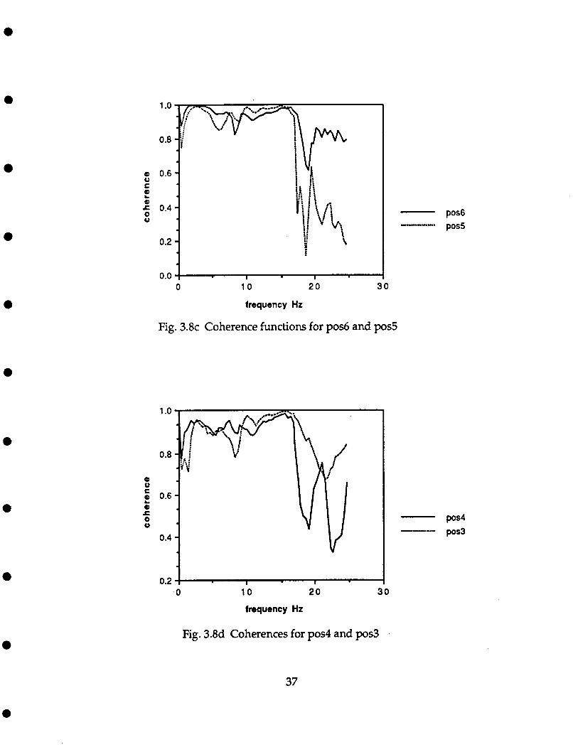
Fig. 3.8 c

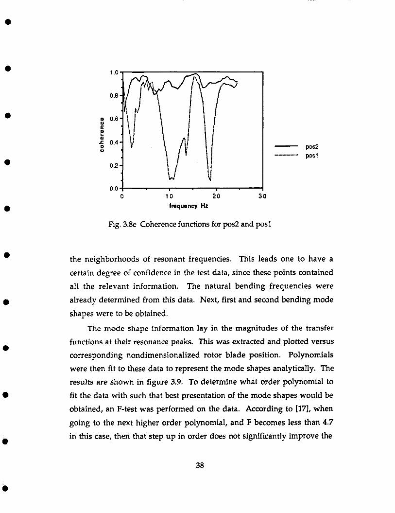
Fig. 3.8 d

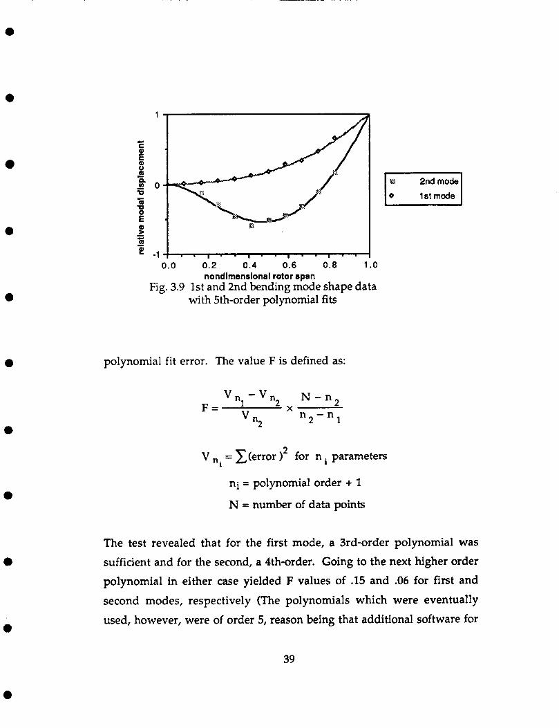
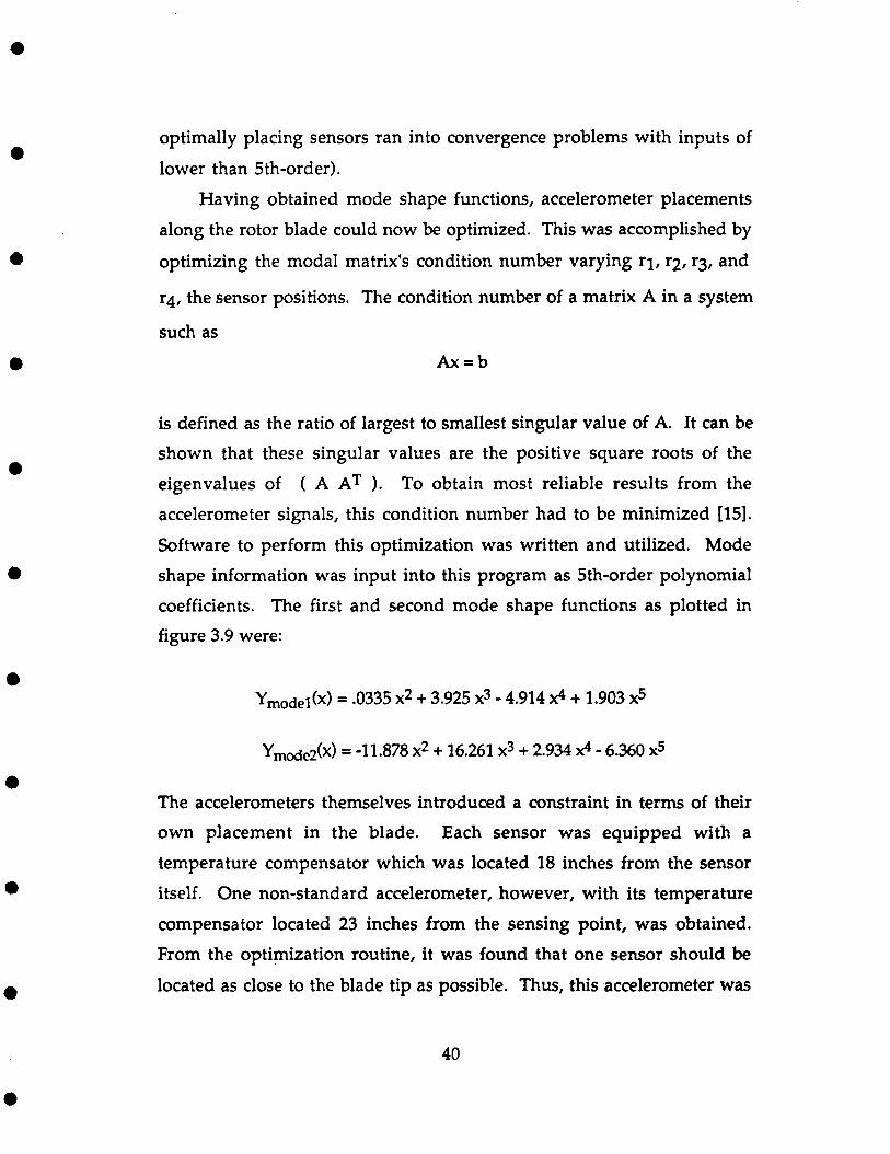
Fig. 3.8 e Fig. 3.9

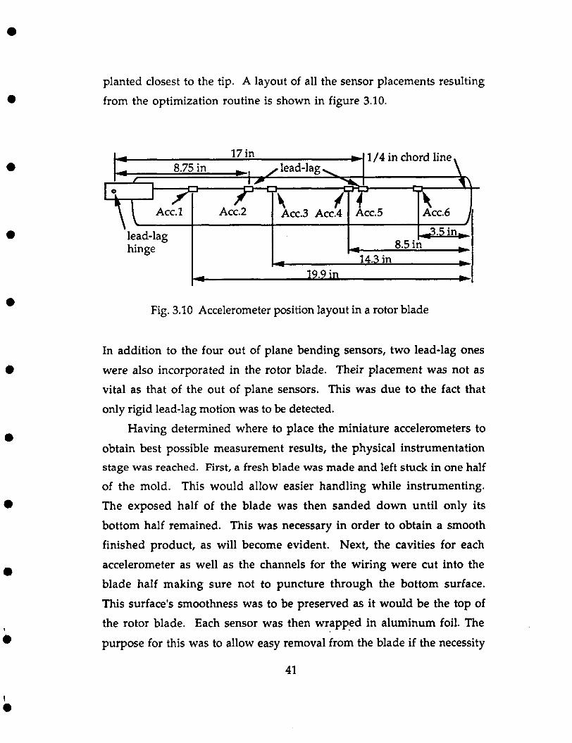
Fig. 3.10

Fig. 4.1 a

Fig. 4.1 b

Fig. 5.1 Fig. 5.2

Fig. 5.3

Rotor blade reaction forces at hinge.

Description of the Princeton Rotorcraft Dynamics Lab.

Data acquisition functional diagram.

Helicopter test model arrangement.

Rotor blade and holder arrangement (side view).

Rotor blade and holder arrangement (top view).

Typical transfer function.

Cambell diagram of rotor blade properties.

Blade accelerometer dynamics.

Impact test locations. Transfer functions for positions 10 through 7. Transfer functions for positions 6 through 4. Transfer functions for positions 3 through 1.

Coherence functions for positions 10 and 9.

Coherence functions for positions 8 and 7. Coherence functions for positions 6 and 5. Coherence functions for positions 4 and 3.

Coherence functions for positions 2 and 1. 1st and 2nd bending modeshape data with 5th-order

polynomial fits.

Accelerometer position layout in a rotor blade.

Model-strain gauge balance adapter setup (side view).

Model-strain gauge balance adapter setup (rear view).

One per rev ramp signal.

One per rev clock.

Forward flight velocity (tachometer output).

Fig. 5.4 Reference blade pitch angle (el).

111

PRECEDING PAGE BLANK NOT FILMED

~

a

0

a

0

e

0

i

i

Fig. 5.5

Fig. 5.6

Fig. 5.7

Fig. 5.8

Fig. 5.9

Fig. 5.10

Fig. 5.11

Fig. 5.12

Fig. 5.13

Fig. 5.14

Fig. 5.15

Fig. 5.16

Fig. 5.17

Fig. 5.18

Fig. 5.19

Fig. 5.20

Fig. 5.21

Fig. 5.22

Fig. 5.23 Fig. 5.24

Fig. 5.25

Fig. 5.26

Fig. 5.27

Fig. 5.28

Fig. 5.29

Fig. 5.30

Fig. 5.31

Fig. 5.32

Second blade pitch angle (e,).

Third blade pitch angle (e,). Tip accelerometer response (acc. 6, out-of-plane).

Accelerometer 4 response (out-of-plane).

Accelerometer 3 response (out-of-plane).

Root accelerometer response (acc. I, out-of-plane).

Accelerometer 5 response (lead-lag).

Accelerometer 2 response (lead-lag). Aerodynamic x-force.

Aerodynamic y-force.

Aerodynamic z-force.

Aerodynamic Roll moment.

Aerodynamic Pitch moment.

Aerodynamic Yaw moment.

Pre-filtered accelerometer output from acc. 1.

Pre-filtered accelerometer output from acc. 3.

Pre-filtered accelerometer output from acc. 4.

Pre-filtered accelerometer output from acc. 6.

First mode displacement estimate. First mode velocity estimate.

First mode acceleration measurements.

Second mode displacement estimate.

Second mode velocity estimate.

Second mode acceleration measurements.

Non-dimensional flap spring coefficient.

Non-dimensional flap damping coefficient.

Non-dimensional first mode pitch forcing coefficient.

Non-dimensional second bending mode spring coefficient.

IV

e

e

e

Fig. 5.33 Non-dimensional second bending mode damping

coefficient.

Non-dimensional second bending mode pitch forcing

coefficient.

Fig. 5.34

V

LIST OF SYMBOLS

0

a

0

a

a

a

a

a

a

C

e

V i

Wi

X

Xd

Y Yd

Xk

Yk

...

...

...

...

...

...

...

...

...

...

...

...

...

...

...

...

...

...

...

2-dimensional lift coefficient curve slope

non-rotating beam frequency coefficient for nth mode

number of rotor blades

blade chord

offset of flap hinge or point of fixity from rotation axis

second mode

ith modal position

ith modal velocity

ith modal acceleration

mass per unit length of beam at root

non-dimensional nth accelerometer location on blade

system input

system output

measurement noise

external disturbances

sting balance voltage outputs

differenced voltage outputs

six degree of freedom vector of model states

differenced force and moment inputs

...

...

... longitudinal cyclic

... lateral cyclic

... Power coefficient

... Torque coefficient

x-force component of kth blade

y-force component of kth blade

VI

e

0

0

0

0

e

0

0

I

0

...

...

...

...

...

...

...

...

...

...

...

...

...

e..

Mjj,n(t) ... Mel(t) ... Mg(t) ... Mg/n(t> ...

Me2(t) ... N ... P ... R ... Rlk ... R2k ... R3k ... U(f) ...

t

Thrust coefficient

bending stiffness of beam at root

F-test value

power spectrum of u

cross-spectrum between u(t) and v(t)

sting balance calibration matrix

frequency response function

blade inertia

Southwell coefficient for the nth mode

zero-offset Southwell coefficient

offset correction factor to KO, model roll moment, rotor length (R) model pitch moment, blade mass, modal sensitivity

matrix

flap spring coefficient

flap damping coefficient

flap pitch forcing Coefficient

second mode spring coefficient

second mode damping coefficient

second mode pitch forcing coefficient

model yaw moment

Power

rotor radius

rotating frame radial force component on kth blade

rotating frame tangential force component on kth blade

rotating frame vertical force component on kth blade

Fourier transform of u(t)

VI1

t 0

U*(f) ... V(f) ... Vni ... X ... Y ...

complex conjugate of U(D

Fourier transform of v(t)

variance for ni parameters

x-force acting on model

y-force acting on model

first mode shape function

second mode shape function

z-force acting on model

z-force component of kth blade

0

Zk ...

first mode

blade lock number

... P

... Y

coherence function between x and y

ith mode shape function ... vi a

pitch angle of kth blade 1.. 'k

... '0 collective pitch command

air density at sea level

solidity

non-rotating natural frequency of the nth mode

0 ... P

d ... 6lN& ...

0 rotating natural frequency of the nth mode ... %

R ... rotor speed (Hz)

azimuth angle of kth blade ... v k 0

a

VI11

TABLE OF CONTENTS

a

0

0

0

0

*

Chapter 1 Introduction

1.1 Motivation

1.2 Background

1.3 Thesis objectives Chapter 2 The Princeton Rotorcraft Dynamics Laboratory

2.1 The facility

2.2 The data acquisition system

2.3 Data collection and manipulation software

Chapter 3 Design of the test model

3.1 Design objectives

3.2 Designing the model

3.2.1 Choosing the helicopter kit

3.2.2 The rotor blades

3.2.3 Powering the model

3.2.4 The servo actuators

3.2.5 Additional model modifications

3.3 Sensor configuration and instrumentation

3.3.1 Accelerometer signal content 3.3.2 Blade accelerometer installation

Chapter 4 Experimental procedure

4.1 Test preparation

4.2 Test procedure

Chapter 5 Results and conclusions

5.1 Resulting data and post-processing

5.2 Conclusions

References

Appendix

6 8

11

14 15

16 16 25

26 27 29 29 32

43

48

50

55 91

93

0 CHAPTER 1

Introduction

e

a

a

1.1 Motivation

For many years research has been going on in an effort to reduce

vibrations in helicopters. There are three main sources of vibrations,

and they can be placed in three categories, low, medium, and high

frequency [l]. The highest frequency vibrations are caused mainly by the

drive train. The medium frequency source is primarily the tail rotor

which typically spins about five times as fast as the main rotor. The

lowest frequency vibrations stem almost exclusively from the main

rotor, and it is because of their low frequency that they are the most pronounced and destructive ones. These vibrations not only cause

discomfort for pilots and passengers, but are also responsible for

shortening the useful life of many components in the rotor system as well as in the fuselage of the helicopter. They lessen performance and in

some instances are the limiting factor in achieving top flight speeds.

Over the years, many different active control methods have been used for tackling this vibrations problem. Probably the most successful

approach so far has been the use of higher harmonic control (HHC) [ZI. In this method, various points on the fuselage, often including the pilots

seat, are instrumented with vibration sensors. These are to detect

vibrations introduced to the fuselage by the rotor system via its shaft.

Then, based on these measurements, high frequency blade pitch

commands are input to the rotor system.

Although HHC

reducing vibrations, a

methods have demonstrated good results

different, more direct technique is suggested

in

in

e

e

a

e

a

this paper, and is directly responsible for the experiment described

subsequently. The objective is to skip difficult dynamic modeling

processes and to identify rotor states directly by instrumenting them.

This process would tackle the vibrations problem at its root, and by using

individual blade control (IBC) based on rotor state knowledge, could

conceivably correct it there. The experiment which was directly motivated by these facts is

described in this paper.

1.2 Background

Vibrations of the helicopter fuselage are the response to oscillatory

forces acting at the roots of the rotor blades. These are transmitted

through the shaft to the non-rotating frame. The periodic forces occur at

l/rev and nb/rev frequencies, where b is the number of rotor blades and

n any positive integer. This phenomenon can be explained analytically

b41. The resulting forces acting on each blade hinge can be represented as

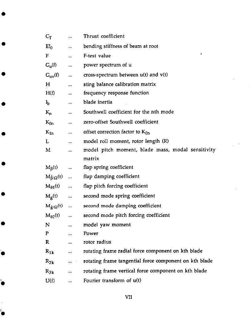
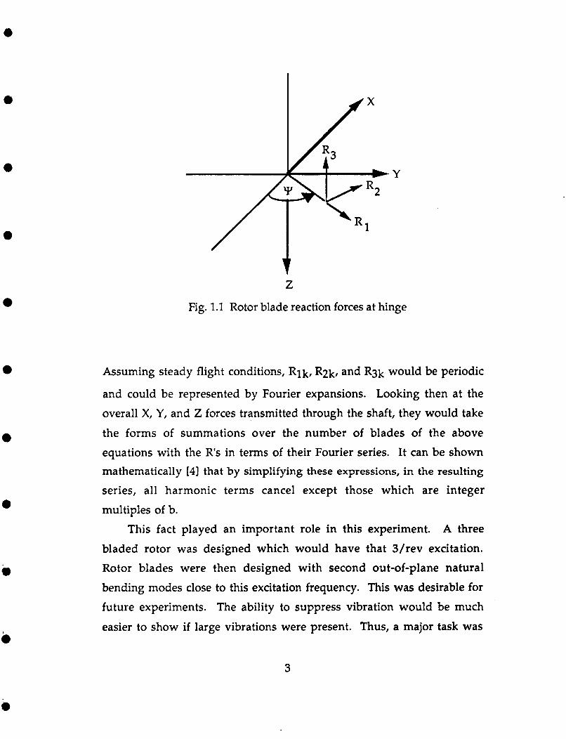
in figure 1.1 by R1, R2, and R3. If Y were the azimuth angle of the zeroth

(reference) blade, then Yk=Y+(2nk)/b would be that of the kth blade.

The corresponding components acting in the non-rotating frame would

then be:

xk= -Rlk COSwk) + R2k Sinwk)

2

e

a

a

i

Z

Fig. 1.1 Rotor blade reaction forces at hinge

Assuming steady flight conditions, Rlk, R2k, and R3k would be periodic

and could be represented by Fourier expansions. Looking then at the

overall X, Y, and Z forces transmitted through the shaft, they would take

the forms of summations over the number of blades of the above

equations with the R's in terms of their Fourier series. It can be shown mathematically [4] that by simplifying these expressions, in the resulting

series, all harmonic terms cancel except those which are integer

multiples of b. This fact played an important role in this experiment. A three

bladed rotor was designed which would have that 3/rev excitation.

Rotor blades were then designed with second out-of-plane natural

bending modes close to this excitation frequency. This was desirable for

future experiments. The ability to suppress vibration would be much

easier to show if large vibrations were present. Thus, a major task was

3

e

e

e

e

a

0

e

e

e

e

0

created, to make a rotor blade with just such characteristics, as well as

insure similarity between the three blades. A process for making the

subject rotor blades was developed and the resulting specimen were

tested for modal properties. The frequency ratios were found to be 3.4

and 1.3 for second and first out-of-plane bending modes, respectively.

Thus, a test operating condition of 8 Hz (480 RPM) was chosen for the

model at which both the first and second natural modes were in close

neighborhood of the 1 /rev and 3/rev forcings.

As mentioned earlier, IBC was to be implemented to control rotor

states in future experiments. This type of control is possible through the

use of a conventional swashplate setup in the case of a three bladed

rotor. If the rotor azimuth angIe were known throughout operation,

then analog sin" and COSY functions could be produced and combined

with desired individual blade pitch angles 01,02, and 03 according to [6]

as:

Thus collective and cyclic commands would be the result and could be

input through conventional actuators to the rotor system. As will be

seen, this was accomplished using a l/rev sensor combined with analog

circuitry.

Using this background information along with other design features, this experiment was conceived. A model was built and tested

in the Princeton Rotorcraft Dynamics laboratory with certain objectives

4

e

e in mind.

e

0

e

1.3 Thesis objectives In order to be able to show in the future that a closed-loop

controller, by using rotor state knowledge, could impact on rotor

dynamics and achieve vibration reduction, a model had to be built and

tested. This was necessary to perform system identification and to verify

that a rotor state estimator could actually yield realistic results based on

the instrumented blade configuration.

Thus, the main objectives of this experiment were to build a usable

model with correct scaling factors, and to test it in the Princeton

Rotorcraft Dynamics Laboratory, which is also described. The model was

to have Froude scaled rotor blades, one of which was instrumented with

six accelerometers. These were used to estimate first and second out of plane bending modal position and velocity as well as first lag modal

position and velocity.

The final step was to do a dynamic test of the fully instrumented

model on the track. This required additional support electronics all of

which are also described in this paper. Actual data and post-processed results showing rotor states as well as parameter estimates are presented.

a

a

5

e

e

e

e

0

e

e

e

e

CHAPTER 2

The Princeton Rotorcraft Dynamics Laboratory

2.1 The Facility

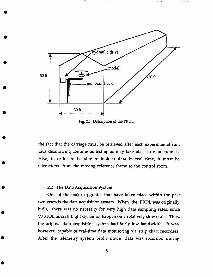
In the mid 1 9 5 0 ’ ~ ~ the Princeton Dynamic Model Track (PDMT) was built for the purpose of investigating aerodynamic characteristics of V/STOL aircraft at slow forward velocities and near hover using

powered Froude scaled models. The PDMT which has since been

upgraded with a new data system is today known as the Princeton

Rotorcraft Dynamics Laboratory (PRDL). It consists of a 750 foot long

metal building with an approximately 30x30 foot cross-section, as

described in figure 2.1. Along one side of the building runs a monorail

track, on which a hydraulically driven carriage rests. The carriage is

supplied with three-phase power which it picks up via brushes along

one of two sets of four rails spanning the length of the track. This source

may be tapped in the form of 400 cycle power at 115 volts AC. It is used

by the drive system as well as any necessary on-board experiment

support electronics. In order to allow mounting of large, heavy models near the center of the test section, the drive system was located on the

near wall side of the track to counterbalance the model weight. Thus,

the system is capable of carrying models weighing up to 60 pounds and

spanning up to 8 feet in diameter at speeds approaching 30 feet/second.

There are two modes of operation at the PRDL. In the dynamic

testing mode, models can be mounted on a ball bearing gimbal support.

Using this setup, any undesirable degrees of freedom of the model may

be constrained, while desirable ones may be left unconstrained allowing

small translational freedom with respect to the carriage. While the

6

a

0

0

0

0

0

e

model is actually moving inside the carriage reference frame, its motions

can be measured. Originally, an on-board analog computer could use

these feed-back signals to accurately position the carriage with respect to

the model. The carriage's dynamic performance is sufficient for

following the model in the Froude time scale [5]. Combining this

arrangement with the capability for precise position and velocity measurements provides a complete system for system identification

[ 6 ] . During static testing, which will be implemented for this

experiment, a model is rigidly mounted on a six-component strain

gauge balance constraining all degrees of freedom in the carriage frame.

The forces and moments acting on it are then measured during an

experimental run at specified conditions. The steel boom to which the

strain gauge balance is attached may be rotated to provide any angle of attack for the model. It may also be interchanged with another boom

allowing models to be mounted and tested in ground effect.

At various points along the track, light bulbs can be installed to act

as light switches to activate or deactivate several functions. For example,

near the end of the track, a light switch disengages the hydraulic drive

system and brakes the carriage. Then it throws it in reverse and retrieves

it at high velocity until another switch is encountered several feet before the control room is reached. This switch again brakes the carriage and

allows a controller to hit a mechanical stop switch. A light switch can also be used to activate smoke release for flow visualization

experiments. The main advantages of the PRDL are low power requirements

during operation of the track, ability to control the models' flight

velocities very precisely, and the removal of all wall boundary layer

effects on the test subjects. Of course, the main disadvantages include

7

0

e

0

0

30 ft

d u l i c drive / /

,model /

rack /

30 ft 4

Fig. 2.1 Description of the PRDL

the fact that the carriage must be retrieved after each experimental run,

thus disallowing continuous testing as may take place in wind tunnels.

Also, in order to be able 'to look at data in real time, it must be telemetered from the moving reference frame to the control room.

2.2 The Data Acquisition System

One of the major upgrades that have taken place within the past

two years is the data acquisition system. When the PRDL was originally

built, there was no necessity for very high data sampling rates, since

V/STOL aircraft flight dynamics happen on a relatively slow scale. Thus, the original data acquisition system had fairly low bandwidth. It was,

however, capable of real-time data monitoring via strip chart recorders.

After the telemetry system broke down, data was recorded during

8

0

0

e

a

e

i

experimental runs on magnetic tape on the moving carriage. At the end

of each testing period, the tape had to be removed from the carriage and

the information on it read into a computer for post processing. This

system did not allow for real-time data monitoring.

Today, however, to make use of the PRDL facility for active

helicopter control experiments such as the one described in this paper,

greater demands are put on the data acquisition system. Signals from the

instrumented blades must be sampled at high rates in order to obtain

accurate rotor state profiles. The rotor in this experiment will be

spinning at approximately 5 Hz during test conditions. Thus for samples

on the order of 100 per revolution, a sampling rate of approximately 500

Hz would be necessary. Also, being able to monitor certain channels in

real time could be very helpful in evaluating experimental runs on line,

leading to more time efficient research. This is a not necessary but

desirable characteristic to have.

Being faced with these new demands, a decision was reached to

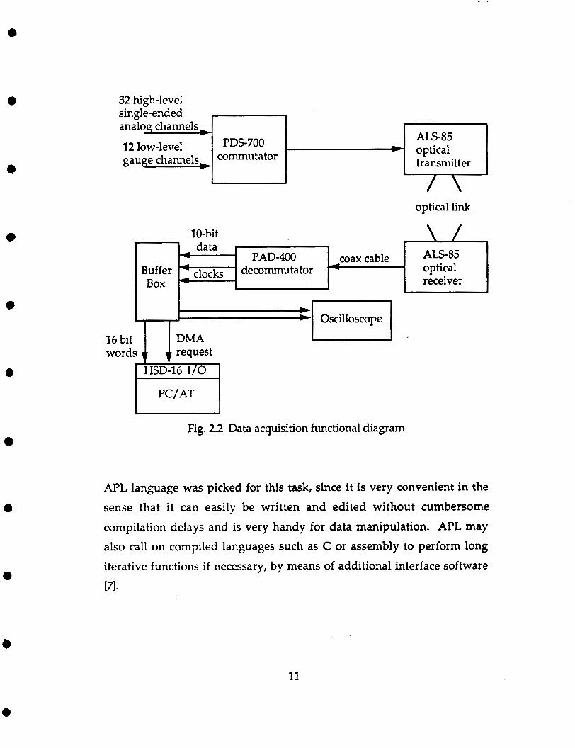
completely replace the old data acquisition system. A functional diagram

of the new system is described in figure 2.2. It is based on the AYDIN

VECTOR PDS-700 commutator and PAD-400 decommutator, both of which are fully documented [9,10]. The PDS-700 unit is capable of simultaneously sampling 44 channels at 1000 Hz each. 32 of these are

high-level single-ended analog inputs while the other 12 are low-level

strain gauge inputs. The commutator converts the 44 signals to 10 bit

words corresponding to a voltage range between -5 and +5 volts. These

words comprise a serial bit stream to the beginning of which two

synchronization words are added. The result is a 46 word frame. This

serial bit stream is then scaled to TI'L voltage levels and fed into the

American Laser Systems ALS-85 optical open-air transmitter [8]. This

unit is mounted close to the supporting rail to minimize any vibratory

9

i

0

a

0

e

noise or misalignment effects. The highly directional optical signal is

shot along the track while the carriage is moving and received by the

ALS-85 receiver which is mounted at one end of the track. (An almost

true monorail combined with accurate aligning sight glasses on each unit allow this type of system to work.) Next, the signal is sent via coax

cable to the control room and into the PAD-400 decommutator box.

From here the data is sent to a buffer card where an additional six

channel identifier bits are added to each word. This buffer card performs

several other functions as well. Two D/A converters and thumbwheels

allow the operator to choose any two channels and look at them in real time on an oscilloscope. A frame clock divide is available to skip chosen

frames of data. In addition, dip switches corresponding to each channel

may be used to turn any unused channels off. These options allow

sampling of data for longer periods of time by not filling the computer

memory with useless information. From this point, data is sent directly

into memory of an IBM PC/AT which is equipped with an HSD-16 card

allowing direct memory access (dma). Using this card, data transfer rates

of up to 120,000 16-bit words per second may be achieved, well beyond

the 46,000 words per second requirement imposed by the PAD-400

decommu t a tor. Two sets of red and green LED's on the buffer box constantly display

the decommutator's major and minor lock status. A green light indicates good lock. Data is read into the PC transparent to the central

processor, such that it may be processed as it is coming in by the

computer. This allows for real time data validity checks, the results of which can be used to adjust any parameters necessary for better results

on line [81.

In order to manipulate the incoming data, a high level computer

language had to be chosen to interface with the HSD-16 1/0 card. The

10

analog channels

12 low-level PDS-700 gauge channels, commutator

e

ALS-85 * optical

transmitter

e

Buffer Box

a

e PAD-400 coax cable ALS-85 data

decommutator optical receiver -,

e

32 high-level

optical link

I I t 1

I Oscilloscope

16 bit DMA words request 7

I HSD-16 1 / 0 1 t 1

Fig. 2.2 Data acquisition functional diagram

0

a

APL language was picked for this task, since it is very convenient in the

sense that it can easily be written and edited without cumbersome

compilation delays and is very handy for data manipulation. APL may also call on compiled languages such as C or assembly to perform long

iterative functions if necessary, by means of additional interface software

171.

e

11

e

e

0

e

0

e

0

2.3 Data Collection and Manipulation Software

Data may be sampled and written in several ways. If relatively few

channels are to be sampled at slow rates such that only 10,000 or less

elements will be written during the run, then this first method will

suffice. While in the APL workspace DMA2APL, the menu driven function DMA must be called. Once it is entered, the operator is

provided with 8 choices, according to which appropriate input data is requested by the program. If multiple channels are sampled at high

rates, memory fills up very fast and much more space may be needed than can be provided in the first method. In this case, APL must be

exited and the program DMA2FILE used. This routine will ask the user

for the number of channels selected, sampling rate, and length of time

data will be collected. It is very important that the response to number of channels coincides with the dip switches on the buffer box. Before data is

written, the DMA trigger ( toggle switch on buffer box ) must be hit to

ensure that it is collected from the beginning of a frame. Once the file is

filled, the user is asked to provide a file name for the data. In this mode, 128 k of elements can be obtained at a time. A third method is available

if sampling rates exceed 500 Hz while every other frame is skipped. In

this case, data can't be written to memory fast enough and the program DMA2PAGE must be used. This program, however, limits the amount

of data taken to 64 k [71.

Once data is written, it can be retrieved and processed within the

APL environment. While in the DMA2APL workspace, the function

GETCHN is used to get data from the file that was written earlier. When

called upon, it requests that filename, the channel number, and the

amount of data points desired. It will then check the top six bits of every

data element and return with the ones corresponding to the given

channel number. If more data is requested than was written, GETCHN

12

0 will return with -1's for excess requests. The function SCOPE is also

available in the DMA2APL workspace. It is a semi-real time digital oscilloscope which can display various channel outputs on the graphics

screen. In adgition to DMA2APL, there are two other available

workspaces, PLOTDATA and SPECTRAL. These contain plotting

routines and spectral analyses tools, respectively. They are fully

documented in reference 7.

e

e

13

a

0

e

CHAPTER 3 Design of the test model

3.1 Design objectives

Several limitations were imposed from the beginning in the design

of the rotor model. One obvious restriction was that of a size and weight

limit imposed by the test facility. Rotor span was limited to 8 feet or less

in diameter and weight to 50 lbs or less. Lack of a full-time professional

staff forced a different approach from the custom model construction

techniques used in earlier V/STOL experiments. Thus, a cost and time

effective method for building a model was sought. Since the objectives

in this experiment pertain to rotor dynamics, the scaling of the rotor

system became vital and that of the fuselage relatively unimportant, so

long as it was scaled in size with respect to the rotor system. Specific characteristics of the rotor blades are discussed in subsequent sections. A

method for instrumenting the rotor blades with sensors which would

yield accurate rotor state measurements had to be developed. - Also, in order to eventually be able to implement adaptive controls on the model, it was desired to have the capability of both individual blade control (IBC) and higher harmonic control (HHC).

These described some of the basic objectives to be met by the model to be tested in the PRDL. More specific requirements are discussed as they were encountered during the actual design phase.

14

0

a

e

0

3.2 Designing the model

To satisfy mainly the time and money constraints, an off-the-shelf

radio control helicopter kit manufactured by Schlueter Inc., West

Germany, was purchased. This type of kit which is readily available

today, has reached a level of sophistication unavailable only several

years ago. It was used as a structural basis for the test model, and is

shown in figure 3.1 along with major modifications.

pitch sensor potentiometers

I 6 1 1 I I I 1 -

hollow shaft I I 1- swash plate a s s e m b 7

1 /rev infra-red emitter

main gear

20 channel slip ring 1 /rev infra-red

detector

structural frame 1 HP DC motor

Fig. 3.1 Helicopter test model arrangement

15

e

e

0

e

e

0

?

e

3.2.1 Choosing the helicopter kit

The model support frame, as shown in the figure, was provided by

the helicopter kit, as was the main gear, swashplate assembly, and rotor

hub. The reason for choosing this model was because of its three-bladed

rotor hub configuration, as well as its size and weight which were well

below imposed limits. A three-bladed rotor was necessary to be able to use IBC without having to use actuators in the rotating frame. As was

explained earlier, IBC can be implemented using a conventional

swashplate setup as long as the rotor system consists of no more than

three blades. This can physically be explained by the fact that the position

of the swashplate in space is defined by three independent points. These,

at any point in time, could conceivably define three independent pitch

commands corresponding to individual blades. It is for this reason that

a blade number less than four was chosen.

The option of a two bladed rotor was also available. The reason it

wasn't taken was so that HHC could be implemented without interfering

with pilot inputs. HHC commands are usually input at (b-l)/rev, b/rev,

and (b+l)/rev frequencies, where b is the number of blades. That means

for a three bladed system, the lowest frequency closed-loop controls

would be input at 2/rev. In the case of a two bladed one, however, this would occur at l/rev. At that frequency, pilot commands are input,

resulting in undesirable interferences in the two bladed rotor case.

3.2.2 The rotor blades

Since the helicopter kit came with a fiberglass fuselage, the size of the model's rotor blades was dictated by the necessity to maintain rotor

to fuselage scaling. Thus, blades needed to be made which would be approximately 2 feet long with a 2 inch chord and display low first and

16

e

a

e

e

a

second bending mode frequencies ( be relatively soft ). With this in

mind, a method for making rotor blades, which would assure

aerodynamic similarity between them, was developed.

To obtain the necessary softness and flexibility for low frequency natural modes, a light weight foam material which could be poured into

a mold in liquid form, was selected. This type of method, which had

been used in past experiments, would also insure similarity between

blades. Following this reasoning, the next step was to make a mold of a

rotor blade with the following dimensional characteristics:

1. 2footspan 2. 2 inch chord

3. NACA 0012 airfoil

4. no twist

5. no taper The airfoil section was chosen because it is a standard symmetrical one

used on vintage helicopters. No taper or twist simplified the process of making a mold. Because much time would go into making this mold, it

was desirable to only have to do it once. This meant making a mold

which could be used many times over without breaking or wearing. To

meet these specifications, a rotor blade mold was machined out of two 3/4 X 3 X 26 inch aluminum slabs using a computerized Bridgeport

milling machine located in the Jadwin machine shop at Princeton University.

The procedure involved writing a program in Anicam (see

Appendix) on a minicam computer which was linked to the mill.

Anicam is a language similar to Basic or Fortran. The program basically

defined coordinates at the tip and root of one half of the blade. It then prompted the milling machine to carve out the material between these

sets of coordinates, using specified cutting tools, spindle RPM's, and feed

17

a

e

a

0

0

e

rates. The procedure of milling was done in steps to assure a smooth

finished surface and due to the large amount of material which had to be

removed. Thus, a rough cut, consisting of two steps, which would mill

to within .01 inches of the final cut, was done first. 14 cuts were made

with a 1 inch ball mill from the trailing edge to 30% chord, milling from

root to tip. Then, 6 cuts with a 1/8 inch ball mill were used to rough cut

from 30% chord to the leading edge. This was necessary because of the

small radius of curvature in the leading edge. Following the rough

cutting, a 1 inch and a 1 /16 inch ball mill were used to make 50 finished

cuts from the trailing edge to 30% chord, and 30 finished cuts from that

point to the leading edge, respectively. Taking advantage of the

precision of the computerized Bridgeport, three aligning holes were then

drilled along one edge of the mold. These were necessary to assure

perfect aligning of the two mold pieces. Eventually, dowels were pressed

into one of the halves and the holes enlarged in the other, allowing for a perfect fit every time.

Due to the many cuts performed by the milling machine, the

process of milling one mold half lasted approximately 2.5 hours. The

resulting pieces displayed very smooth surfaces, although ridges from

the cutting procedure were visible. Using this mold, a procedure for making the actual rotor blades was

devised. A two part polyurethane foam manufactured by the SIG Mfg.

company was acquired. In order to use this product with the mold, a

release agent had to be found which would insure the blade's release

from the mold without braking. After testing several possibilities such

as glycerin, oils, etc., a paste car wax was chosen for its good release

characteristics. The procedure for making a rotor blade consisted of several steps. First, the mold had to be lined with a very thin, uniform

layer of release wax. The next step was to mix the two foam components

18

e

e

e

e

0

e

a

e

a

one part to one. Initially, 18 ml of each component were mixed together

resulting in rotor blades weighing approximately 35 grams. However,

after a 35 gram blade was eventually instrumented, it weighed

approximately 48 grams. As a result, the two non-instrumented blades

had to be made heavier to maintain weight balance. This was

accomplished by mixing 24 ml of each foam component together,

yielding approximately 48 gram rotor blades ( these figures play an

important role in achieving Froude scale characteristics ). The mixing

procedure turned out to be very crucial, as under- or over-mixing

slightly meant less than maximum expansion. This would result in

large air bubbles inside the blade, or simply an incomplete blade. A good

indication that the foam had been mixed the proper amount was when

small bubbles started to form on the surface of the mixture. This would

happen within a matter of about one minute ( one nice characteristic of the foam was that it didn't require external heat to react as was often the

case with products used in the past). Once this point was reached, the

foam was poured uniformly into the mold. It was then quickly closed

and clamped shut with c-clamps to prevent foam from gushing out the

sides. To obtain best results the mold was left overnight to allow curing.

It was found that although the foam hardened in a matter of minutes, it was more advantageous to let it cure for 24 hours. This resulted in

much easier release from the mold. The procedure of retrieving the rotor blade necessitated some carefulness. When slowly prying the mold

open with a screwdriver at specially made slots, attention needed to be

paid to what the blade was doing inside the mold. On one or two occasions a blade was lost because opposite ends were stuck to opposite

mold pieces, resulting in a break when the mold was opened all the way.

After a blade was removed successfully, fine grade sandpaper was used to

smooth the seems which resulted from the molding procedure.

19

e

e

e

e

e

0

e

e

0

As was mentioned earlier, the blades' mass was an important

parameter for scaling purposes. In order to obtain realistic experimental

data, it was very desirable to have Froude scaled rotor blades. Froude

scaling is scaling between aerodynamic and inertial forces. The lock

number ( y ) of a rotor blade, defined as

y=3pacR2/M ,for I b = M R 2 / 3

is the ratio of aerodynamic and inertial forces acting on it. Hence, to

obtain Froude scaled rotor blades, it was necessary for them to have

realistic lock numbers. Full scale rotors usually have lock numbers

between 8 and 13, this defining our acceptable range. As the definition of

y shows, the only freedom to vary once the blade mold was finished lay

in the mass parameter, M. As a result, the blades weighing 35 and 48

grams had lock numbers of 11.4 and 8.3, respectively, both falling within

the acceptable range.

To adapt the rotor blades to the rotor hub, blade holders were

machined from aluminum. These were made as to hold the blades with friction as well as sets of two bolts. This unit in turn would fit into the

blade holding slot of the rotor hub and be held in place by the lead-lag

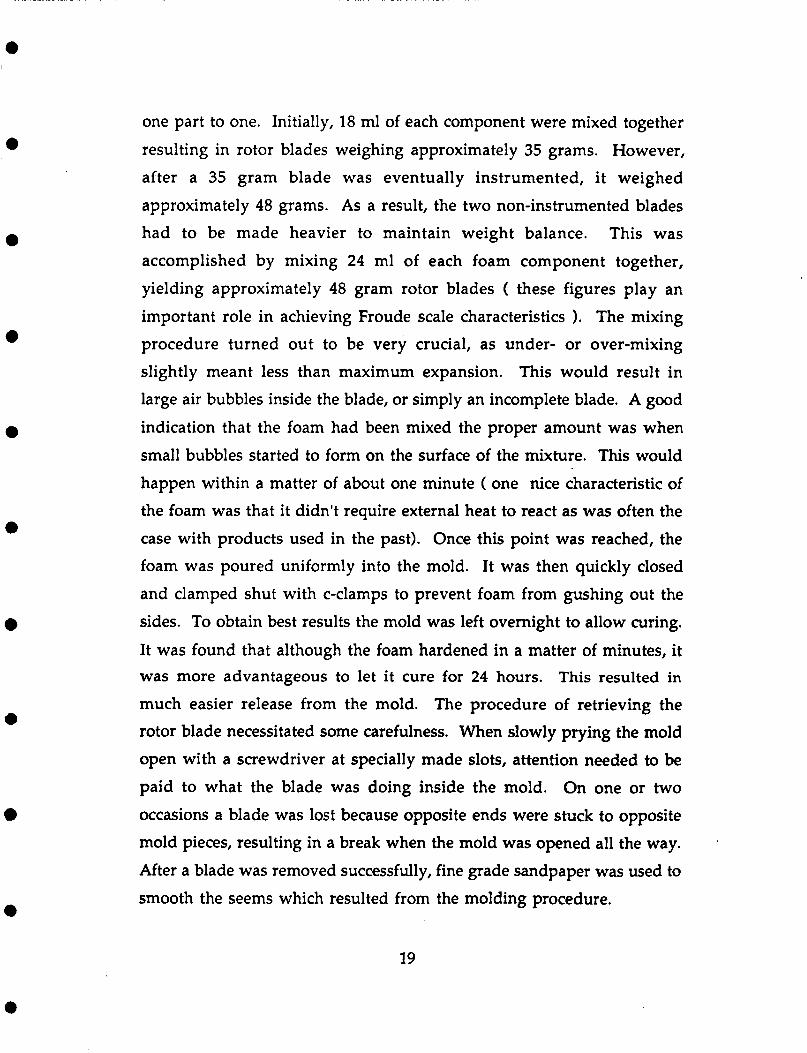
hinge. Figure 3.2 more clearly demonstrates this.

With this blade holder, a rotor blade could now be clamped down

and tested for modal properties. In subsequent sections, it will be shown

that first and second out of plane bending mode shapes become very

important. How they were obtained will be discussed. At this point it

was important to know if the rotor blades possessed low natural

frequencies for these modes, such that good frequency ratios could be

20 .

0

' a

I ' 0

0

0

0

a

13

. . blade holder . . . . . . . . . . . . . . . . . . . . . . . . . . . . . . . . . . . . . . I

r i f t : . : : . . . . . . . . . . . . . . . . . .

1% .-.* ----e .*.... rotor hub

I . . . . - f extension 1 . . 9/4 )I

lead-lag hinge a) sideview

b) topview

Fig. 3.2 a,b Side and top 'views of rotor blade and holder arrangement I

(note: all dimensions in inches)

obtained at slow rotor speeds. To obtain this information, a blade was

clamped down horizontally at its holder for impact testing. This type of

modal analysis technique is thoroughly explained in reference 12. It consists of using a force hammer to create impulse force inputs to the

blade. With a portable PC, the response of a miniature accelerometer,

attached at the tip of the blade, as well as the hammer input, were

sampled at 100 Hz. The transfer function between the output and input

was then calculated and its frequency response plotted. This was done at

21

0

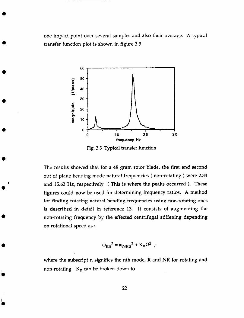
one impact point over several samples and also their average. A typical transfer function plot is shown in figure 3.3.

50

40

30

20

10

0 0 1 0 20 30

frequency Hz

Fig. 3.3 Typical transfer function

0

0

The results showed that for a 48 gram rotor blade, the first and second

out of plane bending mode natural frequencies ( non-rotating ) were 2.34

and 15.62 Hz, respectively ( This is where the peaks occurred >. These

figures could now be used for determining frequency ratios. A method for finding rotating natural bending frequencies using non-rotating ones

is described in detail in reference 13. It consists of augmenting the

non-rotating frequency by the effected centrifugal stiffening depending

on rotational speed as :

where the subscript n signifies the nth mode, R and NR for rotating and

non-rotating. Kn can be broken down to

22

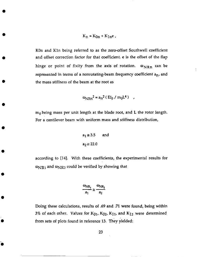
KOn and Kln being referred to as the zero-offset Southwell coefficient

and offset correction factor for that coefficient. e is the offset of the flap

hinge or point of fixity from the axis of rotation. UNRn can be

represented in terms of a nonrotating-beam frequency coefficient an, and

the mass stiffness of the beam at the root as

mobeing mass per unit length at the blade root, and L the rotor length.

For a cantilever beam with uniform mass and stiffness distribution,

e als3.5 and

a2 z 22.0

e

according to [14]. With these coefficients, the experimental results for

U N R ~ and UNR2 could be verified by showing that

Doing these calculations, results of .69 and .71 were found, being within

3% of each other. Values for Kol, Ko2, KI~, and Klz were determined

from sets of plots found in reference 13. They yielded:

23

0

With the offset e equaling .47 feet,

K1 = K01 + K11 e = 1.56

K2 = K02 + K12 e = 8.13.

With these factors known, frequency ratios were determined to be :

a

0

0

a

o (1st bending ) / R = 1.28 and

o (2nd bending) / R = 3.43 at

R = 8 H z .

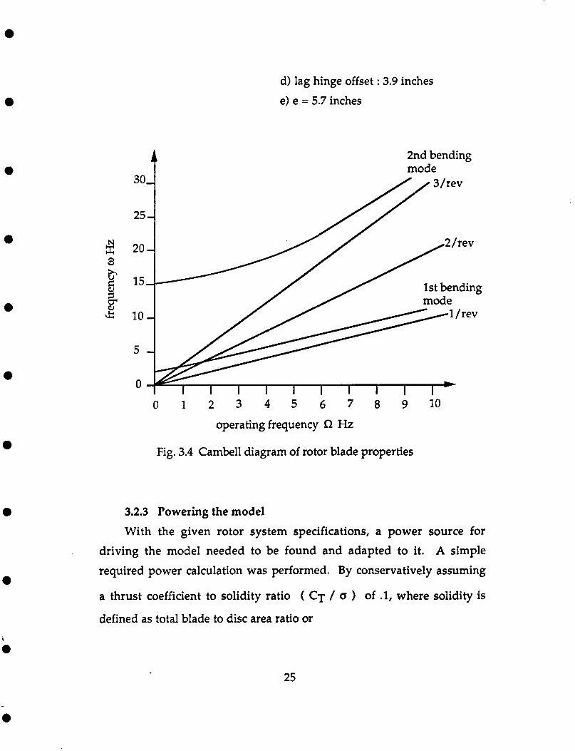
A Cambell diagram which shows approximate modal characteristics of

the tested rotor blade is shown in figure 3.4.

In summary, important rotor blade and hub characteristics are listed

1) rotor blade radius : 2 feet

2) rotor blade chord : 2 inches

3) airfoil section

4) o (1st bending) / R 1.3 (R=8 Hz)

5) o (2nd bending) / R z 3.4 (R=8 Hz) 6) rotor hub configuration:

as follows:

: NACA 0012

a) 3 blades

b) lead-lag hinge c) no flap hinge

24

0

a 30-1

a

0

a

0

3 c f &

d) lag hinge offset : 3.9 inches

e) e = 5.7 inches

2nd bending mode

0 1 2 3 4 5 6 7 8 9 10

operating frequency R Hz

Fig. 3.4 Cambell diagram of rotor blade properties

3.2.3 Powering the model With the given rotor system specifications, a power source for

driving the model needed to be found and adapted to it. A simple

required power calculation was performed. By conservatively assuming

.

a thrust coefficient to solidity ratio ( CT / Q ) of .l, where solidity is

defined as total blade to disc area ratio or

25

C Y = 7c R2

the thrust coefficient was determined to be 0.008.

By using the relationships

a

e

e

CT" '2

' Q = f i c, = CQ

3 P = c p( ~ X R * ) ( RR )

necessary power was determined to be 0.9 HP at 480 RPM. These results

helped in choosing a motor for driving the model. Because operating

speed wasn't anticipated to be much more than 8 Hz, a 1.0 HP, permanent magnet, DC motor was used.

This motor was adapted to the helicopter model by attaching a gear

comparable to the rotor's main gear to its drive shaft. The motor was

then clamped into position against the helicopter's frame as is shown in figure 3.1.

3.2.4 The servo actuators

A set of three servo actuators was used for positioning the

swashplate through pushrod assemblies. Located, as shown in figure 3.1,

were JRS4051 high speed servos manufactured by JR CIRCUS inc. The

setup was such that for lateral cyclic the two outside ones were used and

for longitudinal cyclic, the middle one. Collective commands were

26

i

e

0

e

e

e

achieved with all three servos in combination.

Positioning of these off the shelf radio control (R.C.) actuators was

accomplished with pulse width modulated (PWM) signals. To be able to

input collective or cyclic commands, an integrated circuit (IC) card was

designed. This card was to be carried by a card bus on the carriage. Its job

was to take cyclic or collective inputs and electronically convert them

into three individual servo commands, by generating and controlling

pulses and their widths. Since both pilot as well as closed-loop control

inputs would eventually go through this unit, it comprised an essential

part for future experiments.

To determine these actuators' capabilities, a test was performed.

Again making use of a portable PC, pitch input commands were

sampled, sweeping through a range of frequencies. Pitch responses to

these inputs, measured by pitch sensors, were also sampled. Transfer

functions from this test revealed that the JR servos were effective up to

approximately 3 Hz. For future closed-loop experiments attempting to

reduce rotor vibrations, this would be insufficient.

3.2.5 Additional model modifications Additional modifications to the stock helicopter kit were made in

support of the rotor experimental program. Sensing each blade's pitch angle was a necessity for doing system identification as well as for future

closed-loop experiments. Thus, for each blade, potentiometers were installed on the hub. By using a simple gear drive, pitch angles could be

measured very accurately by ranging the potentiometers through a 30

volt differential ( between +/- 15 volts ).

In order to send signals from the rotating to the nonrotating

reference frame, a slip ring had to be installed. This assembly had the

27

a

0

a

0

capability of twenty channels, a number limited by the size of the rotor

shaft. As was noted in figure 3.1, a hollow shaft replaced the original.

This part had to be machined out of a stock piece of steel, as drilling into

the kit's hardened steel shaft was an impossibility. The procedure for

machining the new shaft consisted of first drilling a hole into a large

piece of steel. Then a lathe was used to cut that piece down, maintaining

the hole as its center. Twenty wires were then installed to conduct

signals from the rotor hub to the slipring base. How these channels were

used will be described in subsequent sections.

Another important modification to the model was the addition of a

1 /rev sensor. This sensor consisted of an infrared emitter-detector pair,

mounted as shown in figure 3.1. Aluminum tubes were used for

alignment as well as light shielding purposes. A small hole was drilled

through the helicopter's main gear, resulting in a pulse once every

revolution. This signal was fed into a phase lock loop card which would

lock on to it. An LED and a beeper were installed to verify this lock. The

card would then perform various functions with the locked-on signal.

The l/rev signal was routed to various locations in support of a host of

timing applications. First, in order to generate the swashplate

commands for Individual Blade Control inputs, the pulse was used to synchronize a sine/cosine function generator as part of the analog

electronics on the swashplate command mixer card. In addition, the

pulse drove a ramp generator that was fed into the commutator as an

additional data channel. This ramp was used as an indicator of lost data

in the telemetry signal, as the reconstructed signal would indicate

discrete jumps in signal level for missing stretches of time-sampled data.

Finally, the pulse was subdivided to provide synchronized sampling

pulses for future use with carriage-mounted digital feedback control

applications.

28

0

0

e

e

a

e

3.3 Sensor configuration and instrumentation

As was mentioned in chapter one, the objective in this experiment

was to build a model whose rotor states could be identified by directly

instrumenting the rotor blades. To be more specific, first and second out

of plane bending modal position and velocity of one of the three blades

were to be determined. To accomplish this, miniature accelerometers

were used. This type of sensor configuration had been successfully used in previous system identification studies of helicopter rotor dynamics [8].

In this reference, first out-of-plane bending mode positions and velocities were estimated during hover using a rotor blade instrumented

with two miniature accelerometers. This experiment demonstrated the

advantages of accelerometer sensors over conventional strain gauges. In

this type of application, strain gauges would encounter serious problems.

When differentiating electronic position signals from the gauge, any

spiky noise would spell disaster. This kind of problem is avoided by

using accelerometers and electronically integrating to obtain velocity and

position estimates.

e

3.3.1 Accelerometer signal content

e

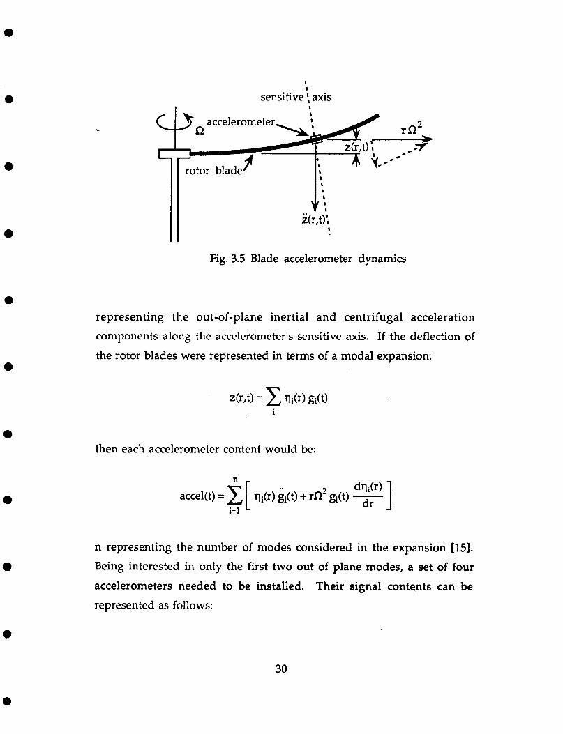
Planted inside the rotor blade, the accelerometers would measure

components of out-of-plane inertial as well as centrifugal acceleration.

Figure 3.5 shows the sensor geometry. According to this setup, the

accelerometers yield:

e

29

e

e l I

sensitive ; axis I

0

Fig. 3.5 Blade accelerometer dynamics

representing the out-of-plane inertial and centrifugal acceleration

components along the accelerometer's sensitive axis. If the deflection of

the rotor blades were represented in terms of a modal expansion:

then each accelerometer content would be:

0

n representing the number of modes considered in the expansion (151. Being interested in only the first two out of plane modes, a set of four

accelerometers needed to be installed. Their signal contents can be

represented as follows:

30

e

e

e

e

e

e

4

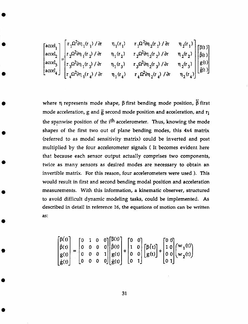
where rl represents mode shape, p first bending mode position, b first

mode acceleration, g and g second mode position and acceleration, and ri

the spanwise position of the ith accelerometer. Thus, knowing the mode

shapes of the first two out of plane bending modes, this 4x4 matrix

(referred to as modal sensitivity matrix) could be inverted and post

multiplied by the four accelerometer signals ( It becomes evident here

that because each sensor output actually comprises two components,

twice as many sensors as desired modes are necessary to obtain an

invertible matrix. For this reason, four accelerometers were used ). This

would result in first and second bending modal position and acceleration

measurements. With this information, a kinematic observer, structured

to avoid difficult dynamic modeling tasks, could be implemented. As

described in detail in reference 16, the equations of motion can be written

as:

31

e

0

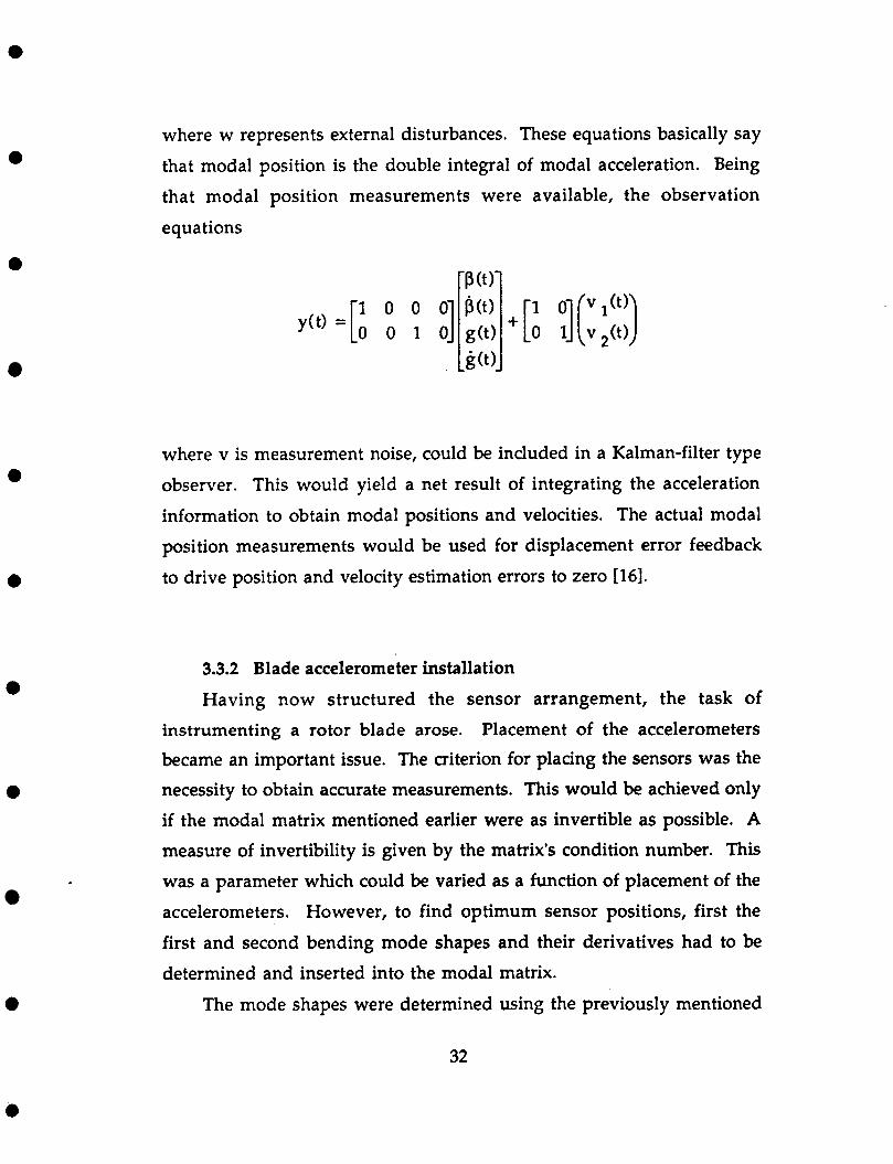
y( t )= [ 1 0 0 0 ] 0 0 1 0

where w represents external disturbances. These equations basically say

that modal position is the double integral of modal acceleration. Being

that modal position measurements were available, the observation

equations

B o > +[I O](Y1(')) g(t> 0 1 v+t>

0

0

0

e

where v is measurement noise, could be included in a Kalman-filter type

observer. This would yield a net result of integrating the acceleration

information to obtain modal positions and velocities. The actual modal

position measurements would be used for displacement error feedback

to drive position and velocity estimation errors to zero [16].

3.3.2 Blade accelerometer installation

Having now structured the sensor arrangement, the task of instrumenting a rotor blade arose. Placement of the accelerometers became an important issue. The criterion for placing the sensors was the necessity to obtain accurate measurements. This would be achieved only

if the modal matrix mentioned earlier were as invertible as possible. A

measure of invertibility is given by the matrix's condition number. This

was a parameter which could be varied as a function of placement of the

accelerometers. However, to find optimum sensor positions, first the

first and second bending mode shapes and their derivatives had to be determined and inserted into the modal matrix.

The mode shapes were determined using the previously mentioned

32

e

e

0

e

mode shape analysis technique [12]. Again, an impact hammer was used

to impart impulse forces along a rotor blade, clamped down at its holder

in the horizontal direction. The response of an accelerometer mounted

as shown in figure 3.6 along with the input force were first sent through

a low pass filter with a cutoff frequency of 25 Hz before being sampled.

This was necessary to filter out unwanted high frequency information

and, in the process, increase data quality. A portable IBM PC then

sampled the data at 100 Hz. Using this data, frequency response

functions H(f) were determined for each impact test as:

where G,,(f) = U*(f) V(f), cross-spectrum between u(t) and v(t)

U(f) = Fourier transform of system input u(t)

V(f) = Fourier transform of system output v(t)

GJf) = U*(f) U(f), power spectrum of u(t)

U+ = complex conjugate of U(f)

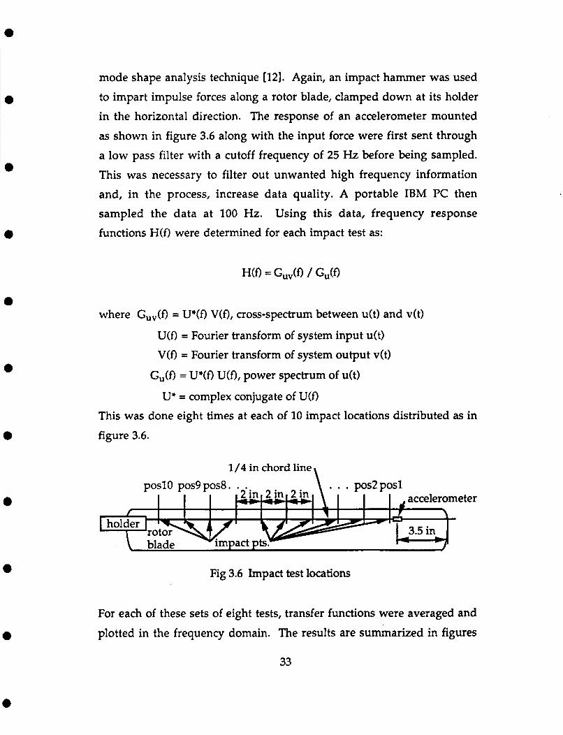
This was done eight times at each of 10 impact locations distributed as in

figure 3.6.

1/4 in chord line

Fig 3.6 Impact test locations

For each of these sets of eight tests, transfer functions were averaged and

plotted in the frequency domain. The results are summarized in figures

33

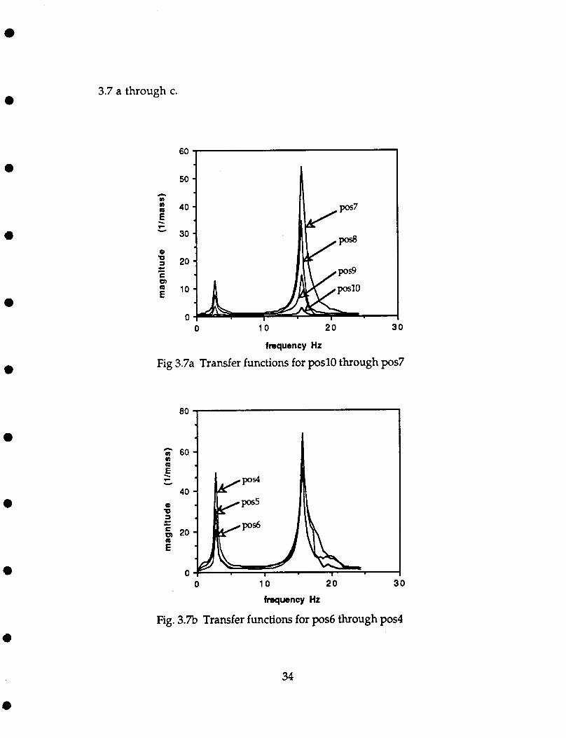
3.7 a through c.

e

e

0

a

n

a a

i \

Y r

al 0

C m

a c - E

60

1 40

30

20

10

0

.

0 10 20 30

fmquency Hz

Fig 3.7a Transfer functions for posl0 through pos7

60

40

20

0 0 10 20 30

fmquency Hz

Fig. 3.7b Transfer functions for pos6 through pod e

34

e

e

e

e

e

e

e

e

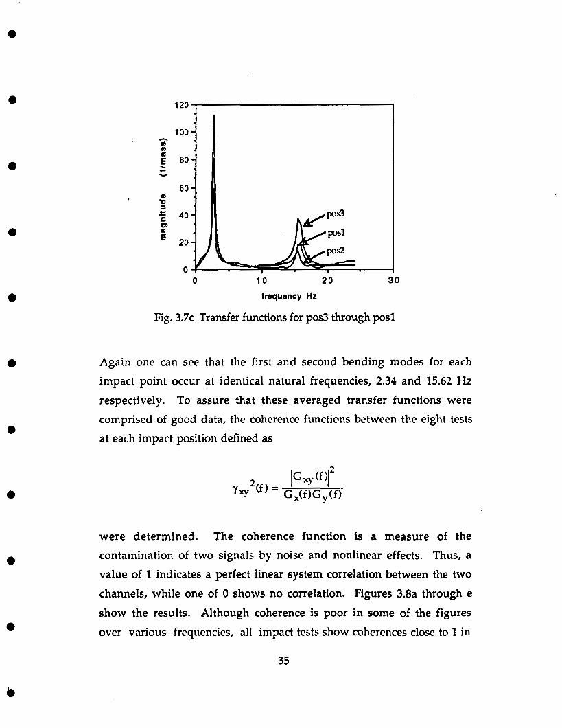
120 1

100 I I A UJ UJ

E \

v- u

0 D

E P,

a c - E

0 1 0 2 0 30 frequency H t

Fig. 3 . 7 ~ Transfer functions for pos3 through posl

Again one can see that the first and second bending modes for each

impact point occur at identical natural frequencies, 2.34 and 15.62 Hz respectively. To assure that these averaged transfer functions were

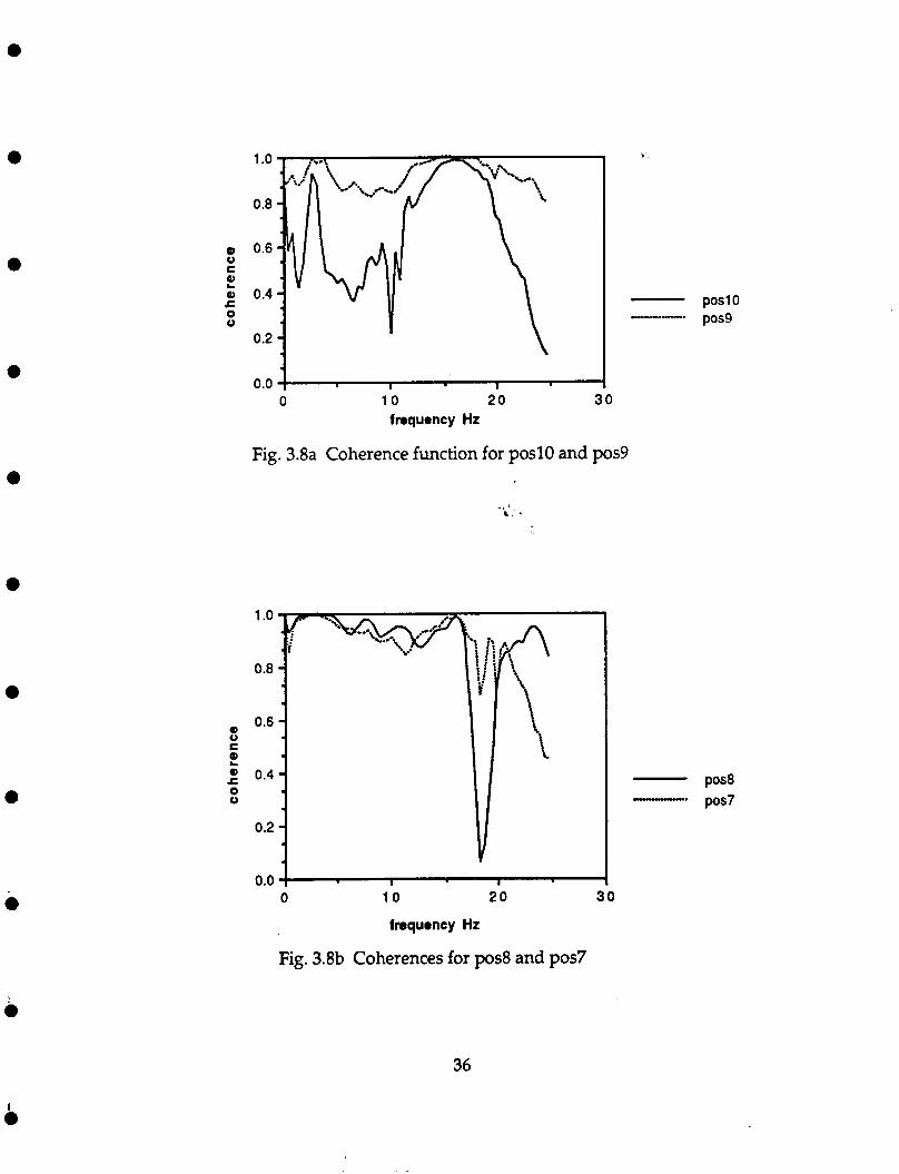
comprised of good data, the coherence functions between the eight tests

at each impact position defined as

were determined. The coherence function is a measure of the

contamination of two signals by noise and nonlinear effects. Thus, a value of 1 indicates a perfect linear system correlation between the two

channels, while one of 0 shows no correlation. Figures 3.8a through e show the results. Although coherence is poor in some of the figures

over various frequencies, all impact tests show coherences close to 1 in

35

a

a

a

0) 0 E

0) t 0 0

2

0 1 0 20 30 frequency Hz

Fig. 3.8a Coherence function for posl0 and pos9

a

0

0) 0 c

9, c 0 0

2?

1 .o

0.8

0.6

0.4

0.2

0.0 ! 1 1

0 10 20 30

frequency Hz

Fie. 3.8b Coherences for pos8 and pos7

p0d0 p059

p058 p057 -...

36

e

0

0, u E

Q, t 0 0

t!

1 .o

0.8

0.6

0.4

0.2

0.0 0 1 0 20 30

frequency H t

Fig. 3 . 8 ~ Coherence functions for pos6 and pos5

1 .o

0.8

0.6

0.4

0.2 1 0 10 20 30

frequency Hz

Fig. 3.8d Coherences for pod and pos3

p056 p055 YI.... " ..

37

e

e

pos2 posl -7".

e

0.8

ai 0.6 0 c

a 0 0

E 0.4

0.2

0.0

e

e

0

0 1 0 20 30 fmquency H t

Fig. 3.8e Coherence functions for pos2 and posl

the neighborhoods of resonant frequencies. This leads one to have a certain degree of confidence in the test data, since these points contained

all the relevant information. The natural bending frequencies were

already determined from this data. Next, first and second bending mode

shapes were to be obtained.

The mode shape information lay in the magnitudes of the transfer

functions at their resonance peaks. This was extracted and plotted versus

corresponding nondimensionalized rotor blade position. Polynomials

were then fit to these data to represent the mode shapes analytically. The

results are shown in figure 3.9. To determine what order polynomial to

fit the data with such that best presentation of the mode shapes would be

obtained, an F-test was performed on the data. According to [17], when

going to the next higher order polynomial, and F becomes less than 4.7

in this case, then that step up in order does not significantly improve the

38

e

0

e

0

e

0.0 0.2 0.4 0.6 0.8 1 .o nondlmenslonal rotor span

Fig. 3.9 1st and 2nd bending mode shape data with 5th-order polynomial fits

polynomial fit error. The value F is defined as:

2nd mode

1 st mode

V n - V n N - n 2 F = 1 2 x

V n 2 " 2 - " 1

2 v ni = C(error for n parameters

ni = polynomial order + 1

N = number of data points

The test revealed that for the first mode, a 3rd-order polynomial was

sufficient and for the second, a 4th-order. Going to the next higher order

polynomial in either case yielded F values of .15 and .06 for first and

second modes, respectively (The polynomials which were eventually

used, however, were of order 5, reason being that additional software for

39

0

e

a

e

0

optimally placing sensors ran into convergence problems with inputs of

lower than 5th-order).

Having obtained mode shape functions, accelerometer placements

along the rotor blade could now be optimized. This was accomplished by

optimizing the modal matrix's condition number varying '1, 1-2, '3, and

r4, the sensor positions. The condition number of a matrix A in a system

such as Ax=b

is defined as the ratio of largest to smallest singular value of A. It can be

shown that these singular values are the positive square roots of the

eigenvalues of ( A AT ). To obtain most reliable results from the

accelerometer signals, this condition number had to be minimized [15].

Software to perform this optimization was written and utilized. Mode

shape information was input into this program as 5th-order polynomial

coefficients. The first and second mode shape functions as plotted in

figure 3.9 were:

e Ymodel(X) = .0335 X2 + 3.925 X3 - 4.914 & + 1.903 X5

Ymde2(x) = -11.878 x2 + 16.261 ~3 + 2.934 >P - 6.360 ~5

a

The accelerometers themselves introduced a constraint in terms of their

own placement in the blade. Each sensor was equipped with a

temperature compensator which was located 18 inches from the sensor

itself. One non-standard accelerometer, however, with its temperature

compensator located 23 inches from the sensing point, was obtained.

From the optimization routine, it was found that one sensor should be

located as close to the blade tip as possible. Thus, this accelerometer was

40

e

0

e

0

m

planted closest to the tip. A layout of all the sensor placements resulting

from the optimization routine is shown in figure 3.10.

lead-lag hinge

d 14.3 in t

4 . .

19.9 in

Fig. 3.10 Accelerometer position layout in a rotor blade

In addition to the four out of plane bending sensors, two lead-lag ones

were also incorporated in the rotor blade. Their placement was not as

vital as that of the out of plane sensors. This was due to the fact that

only rigid lead-lag motion was to be detected.

Having determined where to place the miniature accelerometers to obtain best possible measurement results, the physical instrumentation stage was reached. First, a fresh blade was made and left stuck in one half

of the mold. This would allow easier handling while instrumenting.

The exposed half of the blade was then sanded down until only its

bottom half remained. This was necessary in order to obtain a smooth

finished product, as will become evident. Next, the cavities for each

accelerometer as well as the channels for the wiring were cut into the

blade half making sure not to puncture through the bottom surface.

This surface's smoothness was to be preserved as it would be the top of the rotor blade. Each sensor was then wrapped in aluminum foil. The

purpose for this was to allow easy removal from the blade if the necessity

41

l e

a

e

e

arose. Following this, the accelerometers were carefully placed in

position, facing up for out of plane and sideways for lead-lag. Since 30

wires had to come out of the mold, a small groove was milled into the

other mold half at the root end. Care had to be taken in choosing which

end of the blade to make the root or tip when implanting the sensors.

This would determine which surface would become the top and bottom

of the rotor blade. It was desirable to make the untouched surface of the

blade ( the surface stuck to the mold half ) the low dynamic pressure

surface since this was likely to be the smoother of the two. Once the

sensors were in place, the mold was prepared to be shut. Half of the

usual amount of liquid foam was mixed and poured over the

instrumented half. The mold was shut, clamped, and left over night.

When the blade was finally removed, and seams were sanded off, a

smooth finished product was obtained. The specimen weighed 48 grams

prompting the making of heavier non-instrumented blades to maintain

rotor balance.

e

42

a

l

0

0

l l

e

CHAPTER 4

Experimental procedure

4.1 Test preparation

Several tasks needed to be completed before testing could begin.

The six-component strain-gauged sting balance had to be calibrated,

procedures for which can be found in reference 7. To accurately identify

forces and moments on the model, the 6x6 matrix relating voltage

signals to the six degrees of freedom had to be constructed such that:

0

where y = [ X L M Z Y N IT , x the corresponding voltage signals,

and H the 6x6 calibration matrix. This was accomplished by calibrating

each degree of freedom and keeping track of every input and output

during this procedure. Then, taking the differenced force and moment

inputs and voltage outputs,

over all samples, a least squares estimate of H was to be found by:

This procedure was done, however a small problem was encountered.

After having taken calibration data for the first five degrees of freedom,

43

e

0

e

a

it was realized that the channel carrying the yawing moment had been

switched off the entire time. Due to time constraints and data channel

priorities established for these tests, it was decided to sacrifice its accuracy.

However, the entire H matrix could still be constructed using calibration

data from the last degree of freedom, where the yaw channel was turned

on. This was accomplished as follows. In the matrix equation

B and C were determined with the last set of calibration data by:

e The Hsx5 matrix was determined by neglecting any yaw coupling as:

a

a

0

using data from the first five degree of freedom calibrations. Knowing,

at this point, Hsx5/ B, and C, a least squares expression for A was

determined utilizing the yaw calibration data:

1 where (M) = C- [yyaw - B xs]

Thus a complete H matrix was constructed the result being:

44

0

0

0

a

0

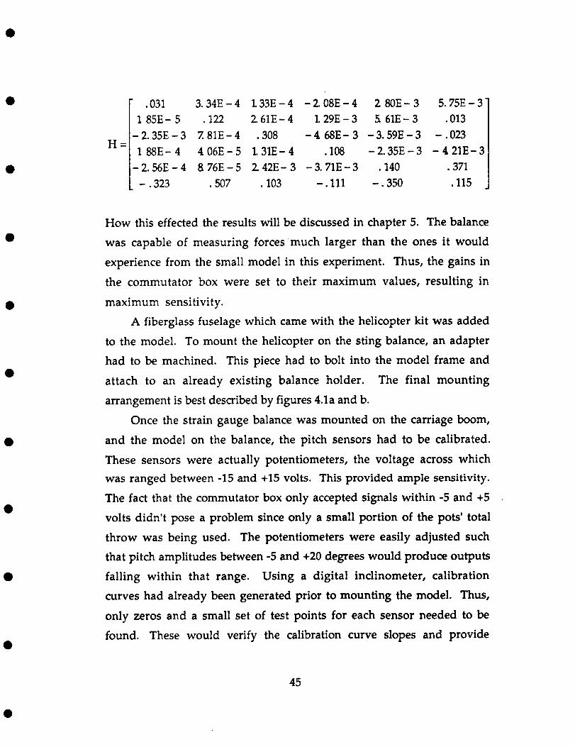
.031 3.34E-4 L33E-4 - 2 0 8 E - 4 2 80E-3 5.75E-3 1 8 5 E - 5 .122 261E-4 L29E-3 5. 61E- 3 ,013

-2.35E-3 Z81E-4 .308 - 4 68E- 3 -3.59E-3 -.OB 1 8 8 E - 4 406E-5 l.31E-4 .lo8 -2.35E-3 - 4 21E-3 H =

- 2 . 5 6 ~ 4 a 7 6 ~ - 5 2 4 2 ~ - 3 - 3 . 7 1 ~ 4 . i 4 0 .371 - .323 .507 . l o 3 - .111 - .350 .115

How this effected the results will be discussed in chapter 5. The balance

was capable of measuring forces much larger than the ones it would

experience from the small model in this experiment. Thus, the gains in

the commutator box were set to their maximum values, resulting in

maximum sensitivity.

A fiberglass fuselage which came with the helicopter kit was added

to the model. To mount the helicopter on the sting balance, an adapter

had to be machined. This piece had to bolt into the model frame and

attach to an already existing balance holder. The final mounting

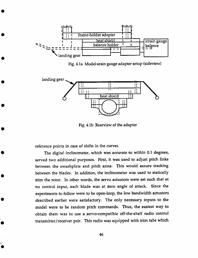
arrangement is best described by figures 4.la and b.

Once the strain gauge balance was mounted on the carriage boom,

and the model on the balance, the pitch sensors had to be calibrated.

These sensors were actually potentiometers, the voltage across which was ranged between -15 and +15 volts. This provided ample sensitivity.

The fact that the commutator box only accepted signals within -5 and +5 volts didn't pose a problem since only a small portion of the pots' total

throw was being used. The potentiometers were easily adjusted such that pitch amplitudes between -5 and +20 degrees would produce outputs

falling within that range. Using a digital inclinometer, calibration curves had already been generated prior to mounting the model. Thus,

only zeros and a small set of test points for each sensor needed to be found. These would verify the calibration curve slopes and provide

45

e

e

0

0

e

0

land ing

Fig. 4.la Modelsrain gauge adapter setup (sideview)

@ m I \

Fig. 4.lb Rearview of the adapter

reference points in case of shifts in the curves.

The digital inclinometer, which was accurate *to within 0.1 degrees,

served two additional purposes. First, it was used to adjust pitch links between the swashplate and pitch arms. This would assure tracking

between the blades. In addition, the inclinometer was used to statically

trim the rotor. In other words, the servo actuators were set such that at no control input, each blade was at zero angle of attack. Since the

experiments to follow were to be open-loop, the low bandwidth actuators

described earlier were satisfactory. The only necessary inputs to the

model were to be random pitch commands. Thus, the easiest way to

obtain them was to use a servo-compatible off-the-shelf radio control

transmitter/receiver pair. This radio was equipped with trim tabs which

46

1

e

e

e

e

e

e

e

were set for static trim.

To transport the sensor signals from the rotor system to the

nonrotating reference frame, their wire leads had to be connected to the

slip ring assembly connectors. Each accelerometer had four wires, two

signal and two excitation voltages. Each pitch sensor had three leads,

one signal and two excitation voltages. Since the slip ring assembly was

limited to only twenty channels, the excitation voltages on both the

potentiometers and accelerometers were made common among each set.

This resulted in nineteen channels being used. The other end of the slip

ring hooked up to a 25 pin connector. A wire carried the signals from

here to the data bus on the carriage. At this point, the accelerometer

signals were picked up by a set of amplifier balances which provided 10

volts of excitation per unit. The pitch sensor excitations were provided

by onboard power supplies. Pitch signals were then fed directly into

channels 7, 8, and 9 of the PDS-700 commutator. To allow lower

sampling rates by electing to skip selected data frames (see chapter 21, a

longer sample period could be achieved. This, however, required the

accelerometer signals to be prefiltered to smooth them out and get rid of unwanted higher frequency information. Thus, the six accelerometer

outputs were first fed through a variable cutoff frequency filter box ( with

fcutoff set at 25 Hz 1, before being sent to channels 10 through 15 of the

commutator.

Other vital information was provided by the l /rev pulse and the

ramp function, which were sent over channels 2 and 3, respectively. The

output of a tachometer, located at the top of the monorail, was fed into

channel 16. This device had previously been calibrated. To obtain

accurate carriage position information, a position sensor was also used.

It consisted of an infrared

bottom of the carriage, facing

emitter/detector pair mounted near the

the near wall; Reflective tape which would

47

0

e

0

e

e

a

0

trigger the sensor was attached at the same level on every support post

along the track. The resulting data from this setup were pulses at exactly

every ten feet of carriage travel. This signal was then scaled to TTL levels and fed into channel 17 of the PDS-700 unit.

4.2 Test procedure

With all vital sensors hooked up and ready, the data sampling stage was nearing. First, the dip switches corresponding to channels to be

sampled on the buffer box were turned on. With the data acquisition

system powered, as well as the card bus and sensors ( carriage plugged

into wall socket ), the model rotor was powered up. This was achieved

with a variac located in the control room. It was connected to two rails

running the length of the track. As was mentioned in chapter 2, there

were two sets of four rails, the lower of which used to power the carriage.

The two rails for powering the model were the lower two of the upper

set. This power, again, was picked up via sets of brushes. Rotor RPM

was adjusted using this variac, with a digital RPM readout available in

the control panel. While the rotor was spinning, each data channel was checked at the buffer box with an oscilloscope. This procedure allowed better balancing of the accelerometer signals. It also verified that all

channels were in working order, and tests could begin.

First, a file of data was written before powering up the rotor. This

would provide a zero for the strain gauge signals. After providing power

to the rotor, and 295 RPM were reached, according to the RPM indicator,

the DMA2FILE program was used to write additional data. Two samples

were taken at hover with no pitch inputs. Two more sets were taken

while inputting random cyclic pitch commands. The next step was to power up the carriage and do forward flight tests. Carriage power up and

48

e

e

rn

0

operating procedures are explained in reference 7. Four data sets were

written, two at flight velocities of 5 ft/sec and two at 10 ft/sec. Two additional sets were taken during transition from hover to forward

flight. The forward flight tests at this point required two operators, one

for carriage control on the track, and the other for data acquisition inside

the control room. It is a future goal to be able to control both these

processes from inside the control room.

After eleven sets of data were successfully written, the first day of

sampling came to an end. The facility was powered down with the

exception of the PDS-700 commutator which was to continue providing

power to the sting balance ( to prevent harmful moisture from

accumulating on it >. Results from this test are described in the

following chapter.

e

l e

49

e CHAPTER 5

Results and conclusions

a

5.1 Resulting data and post-processing

Having made several data runs, enough results were obtained to

verify the usefulness of the model and facility. Some important test

conditions can be summarized as:

1) rotor RPM: 4.05 Hz 2) forward flight velocity : 5 ft/sec 3) advance ratio : 0.08

4) ol(bending) / R = 1.38

5) %(bending) / R = 4.80

a

0

I

0

Figures 5.1 through 5.18 show time histories from the helicopter model

and its rotor. First, a ramp signal verifies that lock of the data

transmission link was maintained, yielding good data in that sense (fig.

5.1). A l/rev clock shows rotor speed to be 4.05 Hz (fig. 5.2). Although noisy, the tachometer signal (fig. 5.3) shows approximately 5 ft/sec flight

velocity. The noise on this signal due to an unknown source occurs at

about 80 Hz. A possible solution to this problem may be to filter the

signal before transmitting it. Figures 5.4 through 5.6 show pitch angles

of each blade. It is important to note that these were input via a radio

transmitter and just happened to be more negative than positive. This fact should be reflected in the measured forces and moments and

actually is in figure 5.15. Here, the z-force, defined positive in the downward direction, is more positive than negative, as expected.

Comparing the plots, it can be seen that the second and third blades lag

50

e

e

e

a

a

the reference blade by 1 /3 and 2/3 revolutions, again as expected. Figures

5.7 through 5.10 are the out of plane accelerometer signals. For reference,

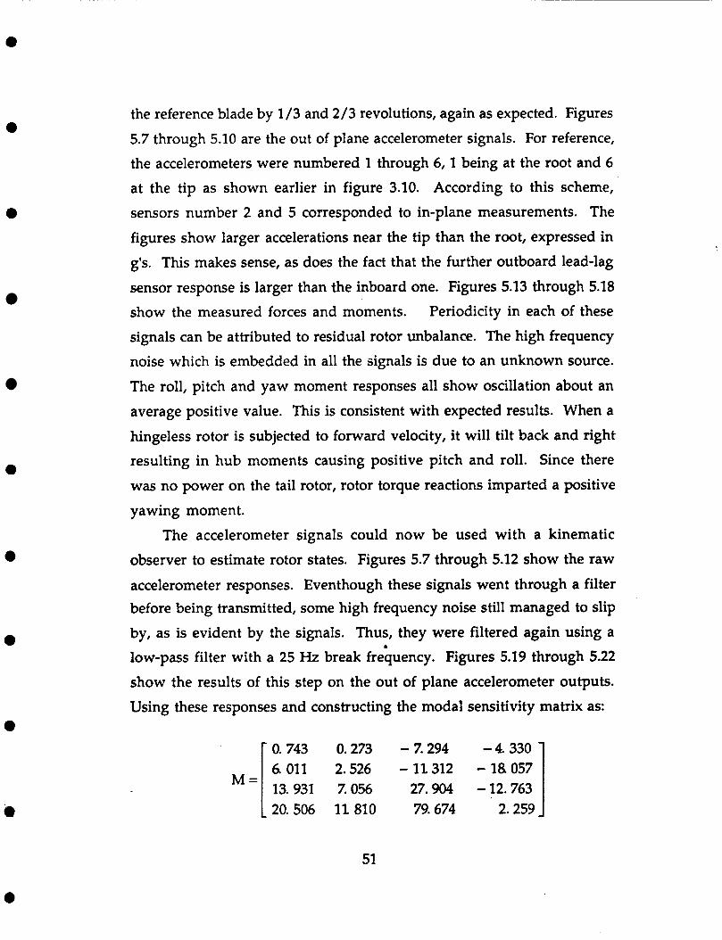
the accelerometers were numbered 1 through 6, 1 being at the root and 6 at the tip as shown earlier in figure 3.10. According to this scheme,

sensors number 2 and 5 corresponded to in-plane measurements. The

figures show larger accelerations near the tip than the root, expressed in

g's. This makes sense, as does the fact that the further outboard lead-lag

sensor response is larger than the inboard one. Figures 5.13 through 5.18 show the measured forces and moments. Periodicity in each of these

signals can be attributed to residual rotor unbalance. The high frequency

noise which is embedded in all the signals is due to an unknown source.

The roll, pitch and yaw moment responses all show oscillation about an

average positive value. This is consistent with expected results. When a

hingeless rotor is subjected to forward velocity, it will tilt back and right

resulting in hub moments causing positive pitch and roll. Since there

was no power on the tail rotor, rotor torque reactions imparted a positive

yawing moment.

The accelerometer signals could now be used with a kinematic

observer to estimate rotor states. Figures 5.7 through 5.12 show the raw

accelerometer responses. Eventhough these signals went through a filter before being transmitted, some high frequency noise still managed to slip

by, as is evident by the signals. Thus, they were filtered again using a low-pass filter with a 25 Hz break frequency. Figures 5.19 through 5.22 show the results of this step on the out of plane accelerometer outputs. Using these responses and constructing the modal sensitivity matrix as:

b

1 0. 743 0.273 - 7.294 -4.330 6. 011 2.526 - 11.312 - 18057 13. 931 7.056 27.904 - 12.763 20.506 11 810 79.674 2.259

51

e

0

e

0

e

0

a

the measurement vector [ p p g g IT was determined. This was done by

pre-multiplying the filtered accelerometer responses by the inverse of

the modal matrix. These measurements could now be used in determining first and second bending mode position and velocity

estimates. Feeding back the error between position measurements and

estimates to the position and velocity estimates and integrating the

acceleration measurements, the desired states were propagated. To use

the position error feedback, feedback gains had to be chosen for all four

states. In the case of first mode position and velocity, low enough gains

needed to be used such that higher frequency information in the

measurements was filtered out. Resulting gains used for these two states

were 3 and 4, respectively, to set the speed of response of the observer to

less than 2/rev. In the case of the second mode, this was not necessary.

Here, the gains used were 30 and 10 for second mode position and

velocity, respectively. Figures 5.23 and 5.24 show the first mode position

and velocity estimates. The position estimates are somewhat suspect.

Realistically, not much more flap position than approximately 0.2

radians was expected. Adjusting the feedback gains may yield better

results. Figure 5.25 shows the actual modal acceleration measurements

which were used in determining the state estimates. The second mode position and velocity estimates are shown in figures 5.26 and 5.27. The

position estimates show more realistic amplitudes, not exceeding 3

degrees. Again, the second mode acceleration measurements used in determining these states are shown in figure 5.28.

Having knowledge now of p, i/Q, p/Q2, g, g/Q, g/Q2, and 8, where

p and g represent first and second modes, the flap equation and bending

equation coefficients from

a

52

?

e

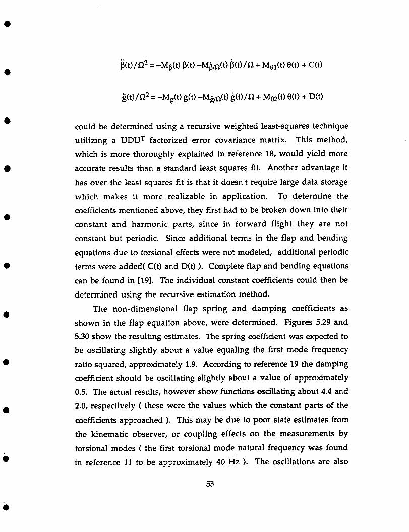
0

0

e

e

0

could be determined using a recursive weighted least-squares technique

utilizing a UDUT factorized error covariance matrix. This method, which is more thoroughly explained in reference 18, would yield more

accurate results than a standard least squares fit. Another advantage it

has over the least squares fit is that it doesn't require large data storage

which makes it more realizable in application. To determine the

coefficients mentioned above, they first had to be broken down into their

constant and harmonic parts, since in forward flight they are not

constant but periodic. Since additional terms in the flap and bending

equations due to torsional effects were not modeled, additional periodic

terms were added( C(t) and D(t) ). Complete flap and bending equations

can be found in [19]. The individual constant coefficients could then be

determined using the recursive estimation method.

The non-dimensional flap spring and damping coefficients as

shown in the flap equation above, were determined. Figures 5.29 and 5.30 show the resulting estimates. The spring coefficient was expected to

be oscillating slightly about a value equaling the first mode frequency

ratio squared, approximately 1.9. According to reference 19 the damping coefficient should be oscillating slightly about a value of approximately

0.5. The actual results, however show functions oscillating about 4.4 and

2.0, respectively ( these were the values which the constant parts of the

coefficients approached ). This may be due to poor state estimates from

the kinematic observer, or coupling effects on the measurements by

torsional modes ( the first torsional mode.natura1 frequency was found

in reference 11 to be approximately 40 Hz 1. The oscillations are also

53

i

e

e

e

much larger than expected. The first mode pitch forcing coefficient as

shown in figure 5.31 was expected to oscillate about a value of about 0.5 according to reference 19, but didn't. In this case, the oscillations were

about a value of approximately 0.1.

From bending equations in reference 19, non-dimensional second

mode spring and damping coefficients were expected to oscillate about

values of approximately 16 and 0.6, respectively. Figures 5.32 and 5.33, however, show disagreement with these values. The constant part of the estimated spring coefficient settled down at an unrealistic value of about

-0.4 while that of the damping coefficient approached 0.003, nearly zero.

Oscillations of the damping coefficient were expected to be between about

+/- 0.05. Actual results oscillated at larger amplitudes. The second mode

pitch forcing coefficient was expected to oscillate with an amplitude of

between approximately +/- 0.01 about a value of approximately 0.5 [19]. The actual results oscillate with about double that amplitude about a

value close to zero, 0.004.

Although not totally obvious from the figures, almost all the

constant parts of each estimated coefficient had not actually settled to

constant values at the end of the estimation routine. Thus, it may be

possible to increase quality of the results by simply allowing more time

for the estimates to settle down.

There are a number of other possible causes for why the resulting coefficient estimates didn't agree with theory. The fact that the flap

position estimates were suspect to begin with is only one. The quality of results for this state estimate could possibly be increased by using more

optimal feedback gains in the kinematic observer. The same goes for the

other states as well. By not modeling any pitch accelerations due to blade

lead-lag in the sensor geometry, the actual measurements may become

suspect. Thus, another solution to the problem may be to include that

54

i

component in the sensor geometry.

e

a

0

a

1

5.2 Conclusions

Having performed the tasks discussed in this paper, several

conclusions may be drawn:

(1) The data acquisition system upgrade at the Princeton

Rotorcraft Dynamics Laboratory has made high speed data sample rates

possible as well as real-time data monitoring. These are two essentials

for performing any type of high frequency active helicopter control

experiments.

(2) Froude scaled model rotor blades were made yielding

frequency ratios of 1.3 and 3.4 for first and second out-of-plane bending

modes at R = 8 Hz, respectively. Active control experiments in the

future, however, will likely require a rotor speed of approximately 5 Hz, in order to reduce necessary sampling and actuator bandwidths. To achieve frequency ratios near 1 and 3 for the two bending modes at lower

RPM, tip masses or distributed masses could be added to the existing

blades. Another way to obtain the natural frequencies would be to find a new, softer material for making the blades.

(3) Current actuators' bandwidths were too low for active

control, however, they were sufficient for trimming the rotor and providing a means for introducing random pitch inputs into the model.

For the rotor spinning near 5 Hz, a useful actuator will be expected to be

able to input +/- 1 degrees of pitch at a minimum of 20 Hz. Thus, the search for a more capable actuator will continue.

(4) Very time- and cost-effective methods for making scaled

rotor blades and constructing a helicopter test model were developed.

Lack of a professional full-time staff for making the test articles forced

55

e

this kind of approach.

(5) Experimental data show that rotor states can be estimated using accelerometer mounted rotor blades. Quality of the results may

possibly be improved through optimal feedback gain computations in

the kinematic observer or by including pitch acceleration in the sensor

geometry. Since the point of this experiment was to illustrate the data

capabilities of the model rotor, lots of fine tuning can be done to the

process to yield better results. These state estimates could then be used to

do more accurate system identification using the procedures discussed.

e

e

56

e

n 0 W u) Y

VOLTS

57

0 ul

T A

Y u 0 J u > W U

tI W a LJ z 0

cu ln

c3 H LL

-7 L -.

I I I I 9 tu 0

I I------ CD

0

W SZ t-i t-

';t

0 .

0

VOLTS

58

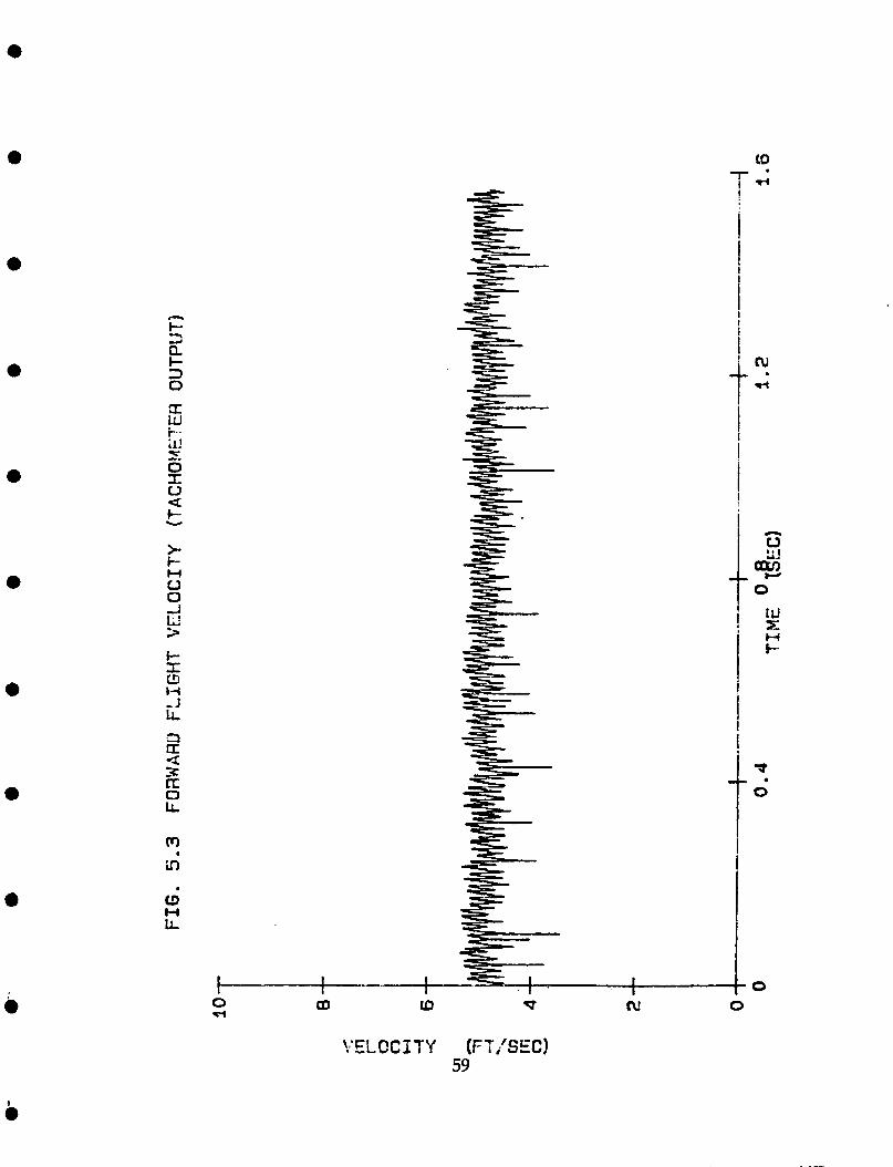
e

a

0

e

e

a

a

a

n

4 k 3 0 X itl

H ij 0

m in

a H 1L

.

.

I------+ 0 Q) tD 4

!.'EL C C 5 TY

P

(FT/SEC) 59

t N

I

t r

ILI x,

!- H I

0

rl

4 i- W I i- U

s w

H R

43- -+-+-5L P I 43 I r(

I 0

P

ANGLE (DEGREES)

60

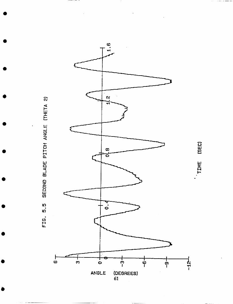
0

e

0 F-" Y

w

1 0 t- H n

a

0 W Ln Y

ANGLE (DEGREES) 61

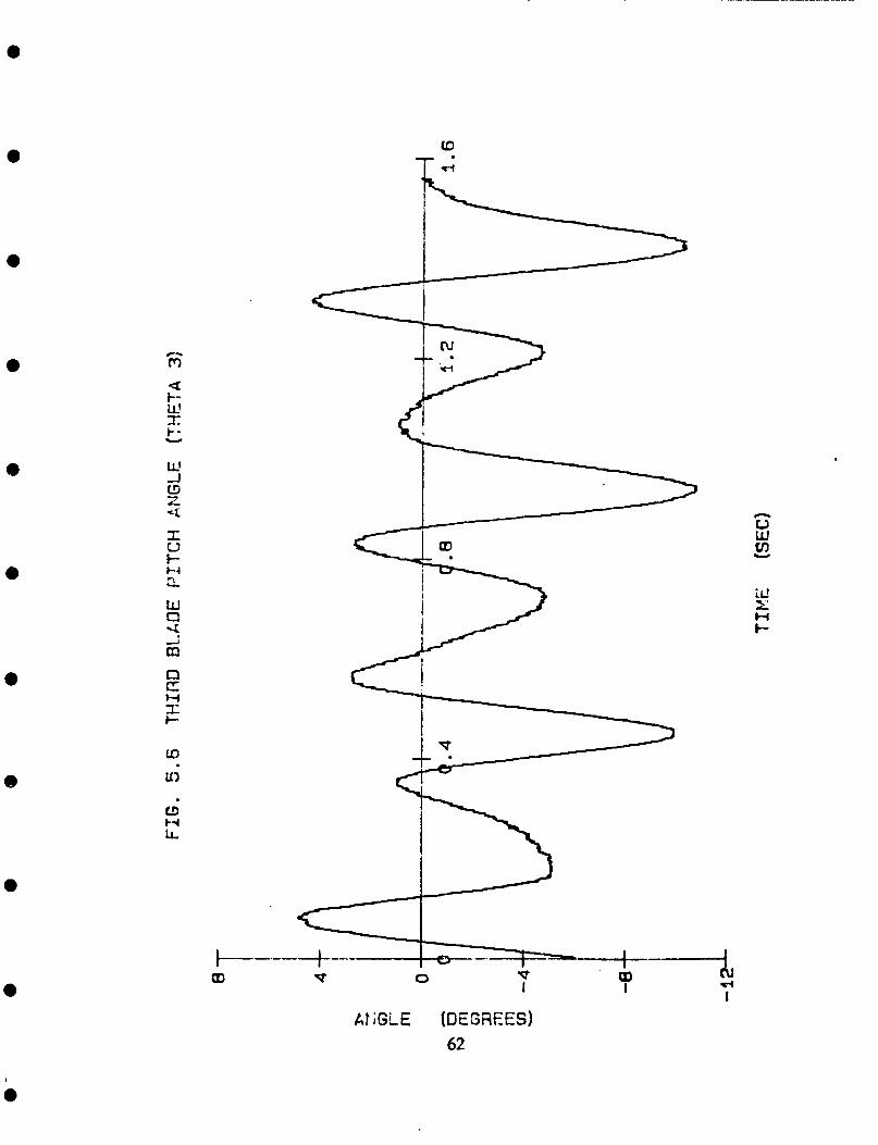
I- c I-4

Lo

It’)

t--- a0 0 .ir

I

H t-

kt ;GLE [DEGREES) 62

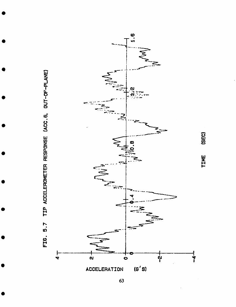
e

P W I N 0

ACCELERATION (G' S)

63

h

W z J I lL 0

I I- 3 0

a a

Y

-- * I - I

W m z 0

m W U

n

n 0 W v) Y

--, = P W x

H t-

a W c, i

-- 1s - a

L3 H LL

1 -- I- -

I cu 0 *

I cu

I m

I

ACCELERATION (G'S)

64

n W z 4 J

I LL 0

I I- =, 0

n

Y I -- c

.c. a %- E-

--

-- I - - 4 0 r)

I

a 0 W ul Y

ACCELERATION (0's)

65

i

h W z J

I LL 0

I I- 3 0

a n

4 . 0 u U

W v) z 0

v) W U

W I- W x 0

W

0 0 4

I- O 0 U

0 r(

v)

Y

a

a

a id

8

r( th 0 0

ACCELERATION (G'S)

8 H I

0 I

I

66

1 I 2 Y Y W v) z 0

c n - W U v)

n

U W I- W z 0 U W 1 w 0 2 4 4

v)

c9 H LL

c -.-

.--

ACCELERATION (G'S) I

n

0 W v) Y

W r H c

r)

I

67

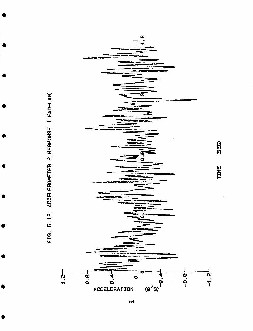
b

(3 a -i' 9 W J Y

e

W cn z 0

cn W U

n 0

n 0 W v1 Y

N

U W + W L 0 U

W 0 Y 3

Y H t

N r(

ln (3

a

W

-- - I I L A

0 Y a

W

0 0 0

ACCELERATION (G'S) 0 I

68

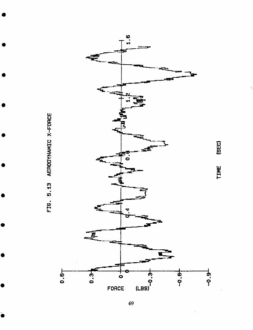
a

10 T d

0

0 H

0

-7r E- / * f

I

-... - _- -e 4- -

0 0

FORCE (LBSI' 0 I

0 I

n 0 W v1 Y

69

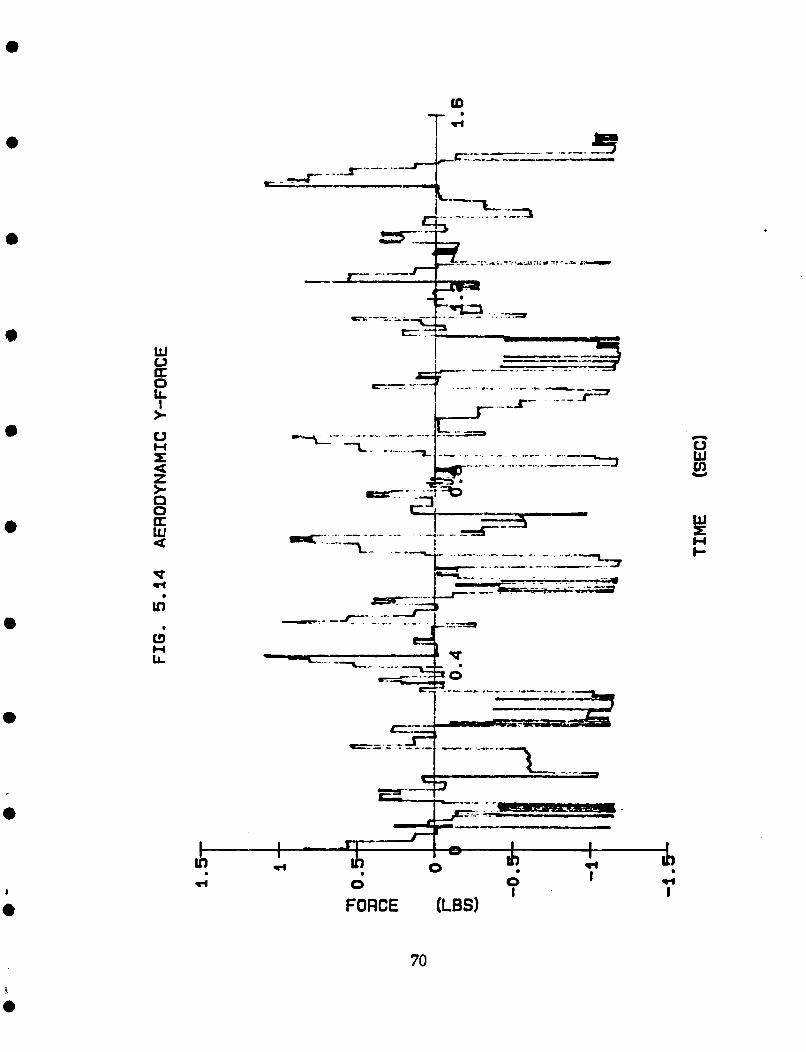
W 0 U 0 LL

I *

a a 0

W <

J

0 H f : 4 t

P

#

4 b

e

a H t

\--

W r W e

FORCE (LBS) e .

70

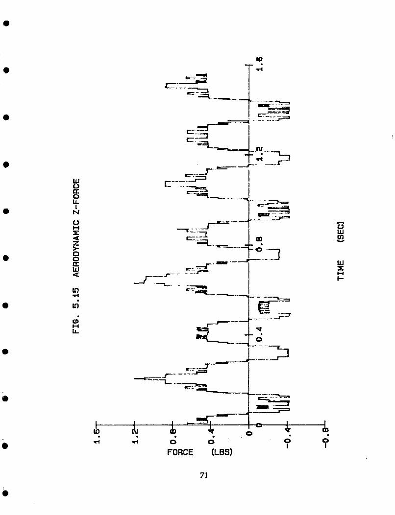
a

I I I -.c-

c-. - --

Ir --- -----Is=

Y - I

a

T" I

I

c. -- I I

0 -2 ----- 3

I-; -3 -.L -.--.+--

e li

I N

L

In

In

c3 H tL

r(

i

0 0

FORCE (LBS) 0 I

0 I

71

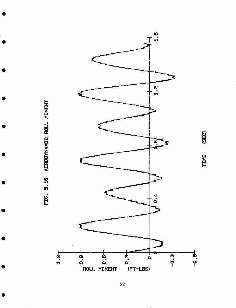
0

a

0

0

J J 0 a

4

dl Ib ci, . 0 0 0

ROLL MOMENT (FT-LBS) 0 I

0 I

72

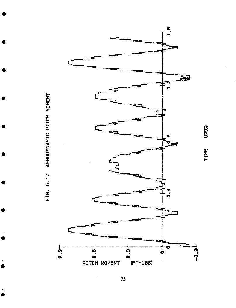
0

I- *

0

e

0

\-.-

e-

0 0 0

PITCH MOMENT (FT-LBS)

73

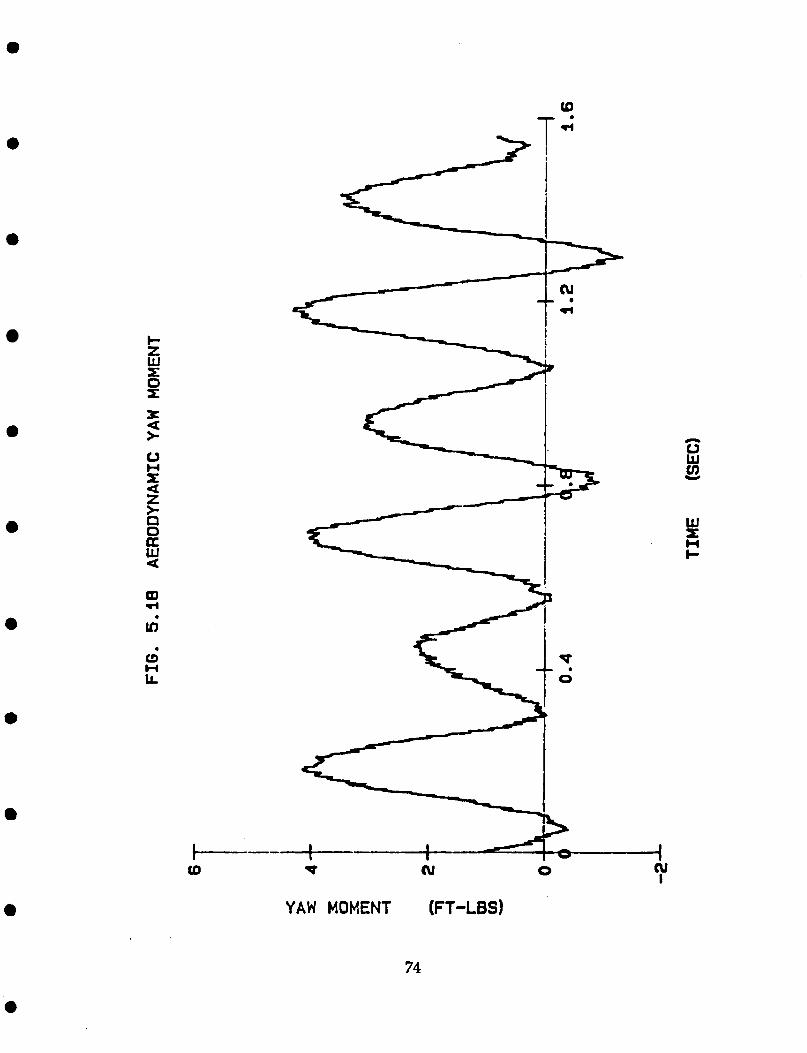
OD rl

W 2:

P 0 \+ '

l--------+----t- Lo 9 ru 0

YAW MOMENT (FT-LBS)

74

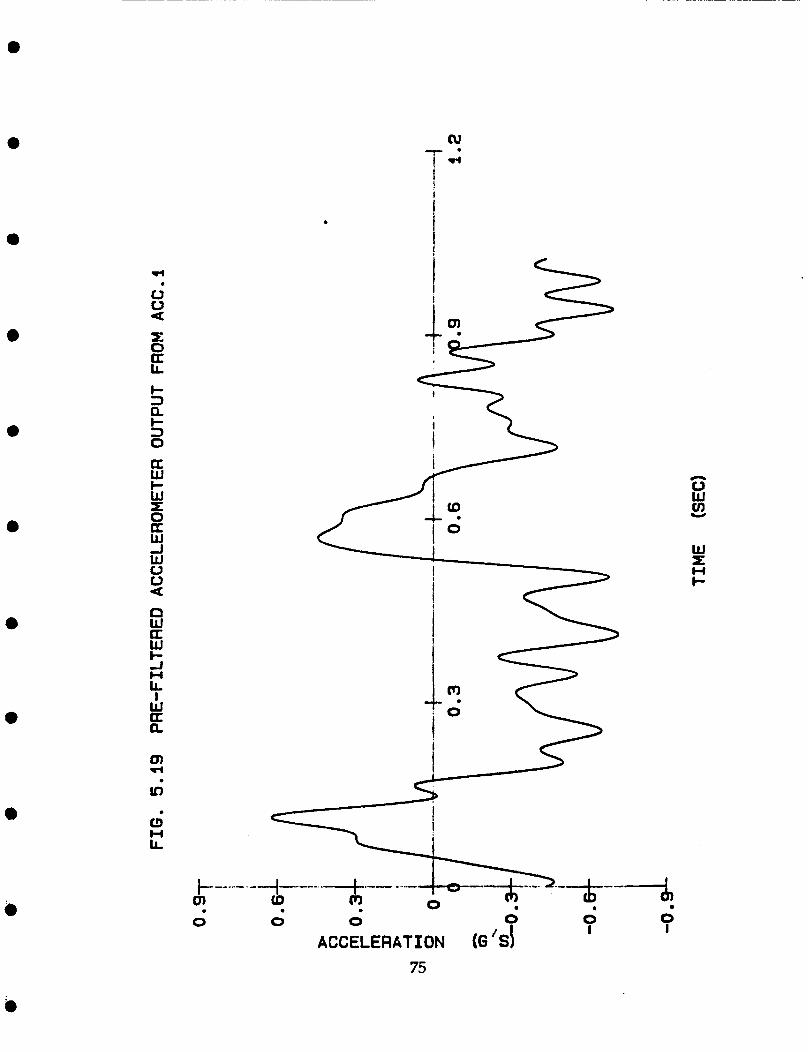
a

a

(u

I

4 .

LL

t t

w I- J H LL

I W pc e

0 I 0 0 0 0

I ACCELERATION (G ‘S\

75

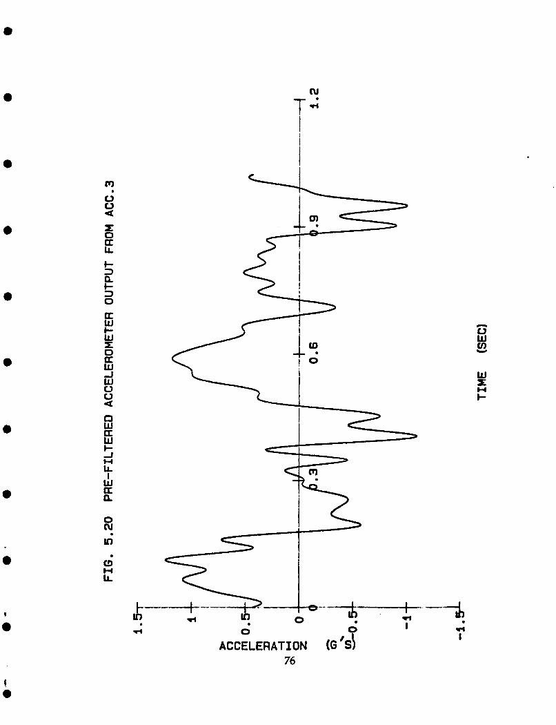
a

0

0

t

m 0 u 4:

P 0 U LL

I- 3 0, t- 3 0

U W I- W r 0 U W J u 0 0

0 W U W t -I H LL I

W U

.

a

n

0 cu IC)

(3 H LL

.

I-

--%* r) I

76

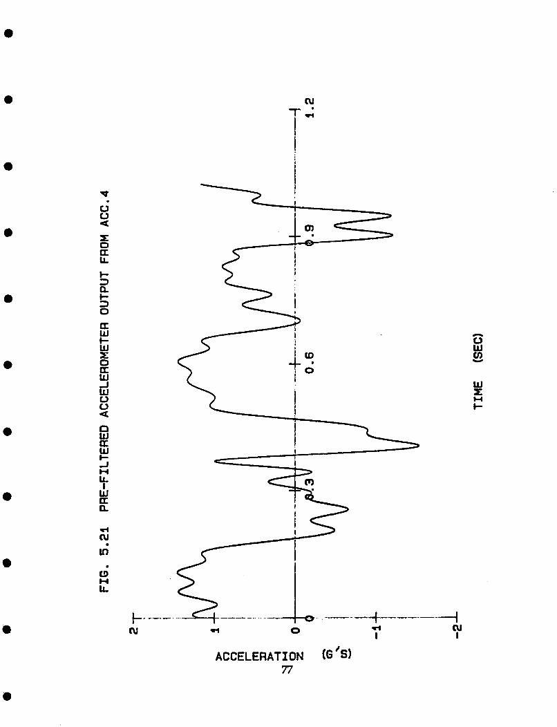
0 0 a

LL c

d 0

r( cu In L3 H LL

.

r4 I r4 0

ACCELERATION @'SI 77

n 0 W u) Y

W r:

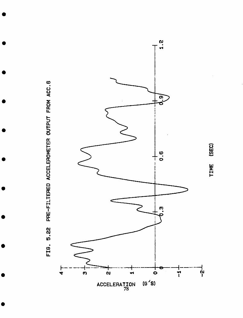
a

I

l

a

a

0

a

e

0

0

to 0 0 U r 0 [I LL

I- 3 a t- 3 0

U W t- W t 0

W J W 0 0 4

0 W U w

.

a

3 H LL

I W

Q.

tu cv It)

t3 H Ir.

a

t-- P

+ x I

t

I -+.----+-.---.- -i

d N I I 0 cu rl 0

ACCELERATION (G 'SI 7Q

n 0 w u) Y

W I: H c-

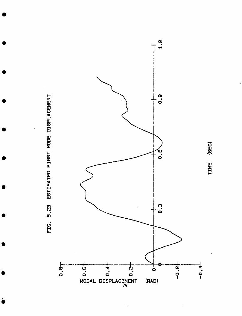
e fu

e

a

a J Q. v)

0 H 0

0 w l-

z H I- v) W

a

+--- OD

0 0 I

0 I 0 0 0

MODAL DISPLACEMENT (RAD) 79

i i 0

0 I 0 0 0

MODAL DISPLACEMENT (RAD) 79

n 0 W v1 Y

W 5 I- H i

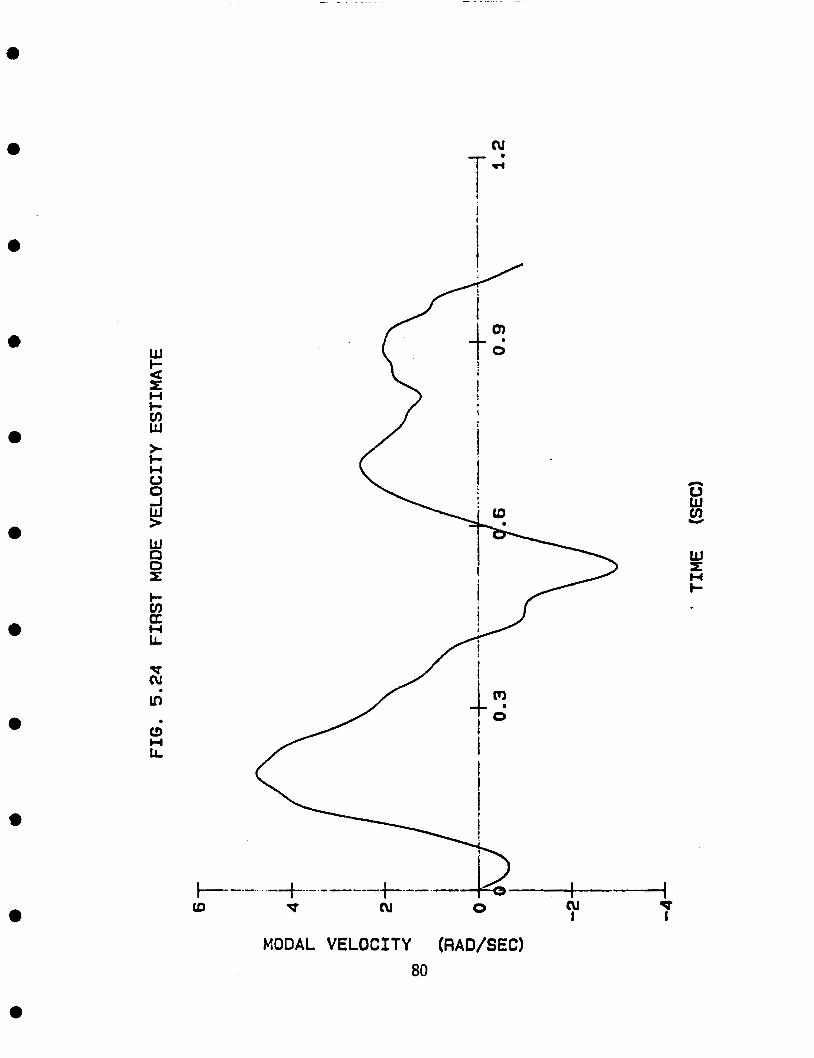
e

0

0

*

0

w t-

in W

v (u

It)

L3 H LL

.

.

t-- ID

MODAL VELOCITY (RAD/SEC) 80

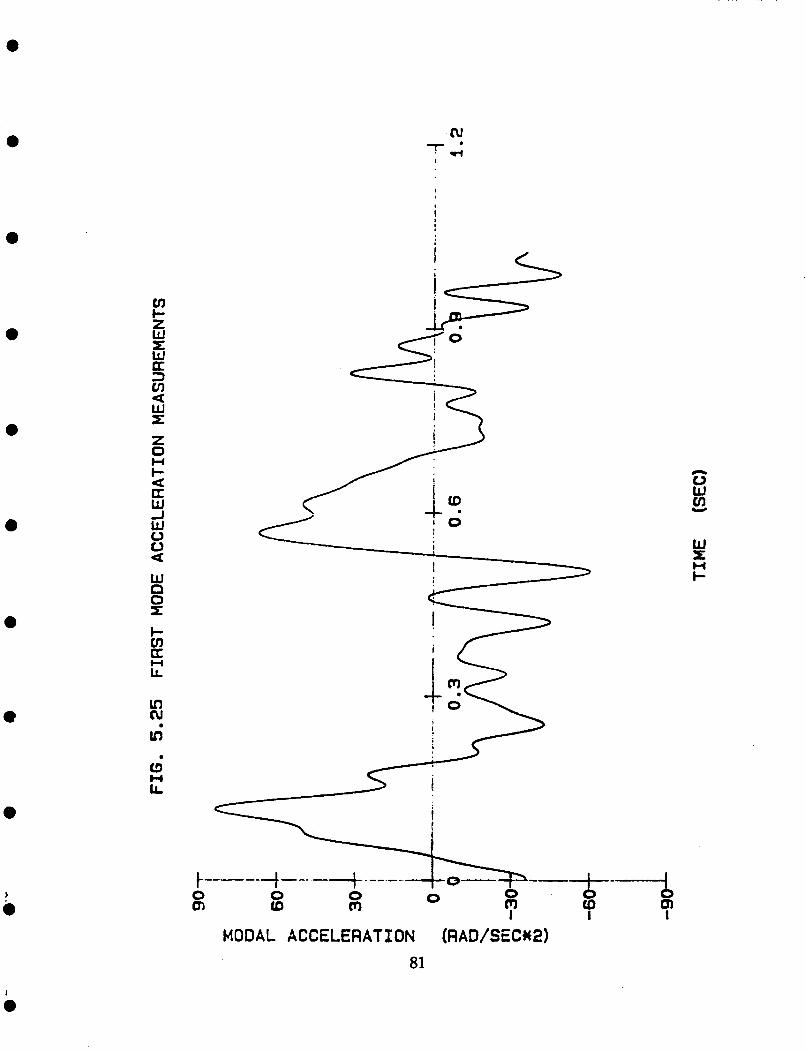
a

a

nl T,'

I

I !

z 0 W c

a

I- cn U Lr. H

In a L n

I-

--% (11

MODAL ACCELERATION (RAD/SEC*2) 81

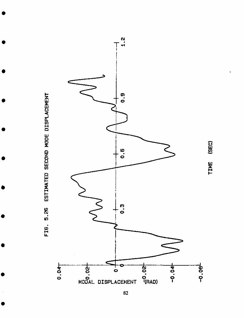
e

0 cu

7-4 !

I 0

e

e

e

0 . 0 0 0

n 0 W cn Y

I-

O 0 0 WO?AL DISPLACEMENT '(RAD) I 0 I

82

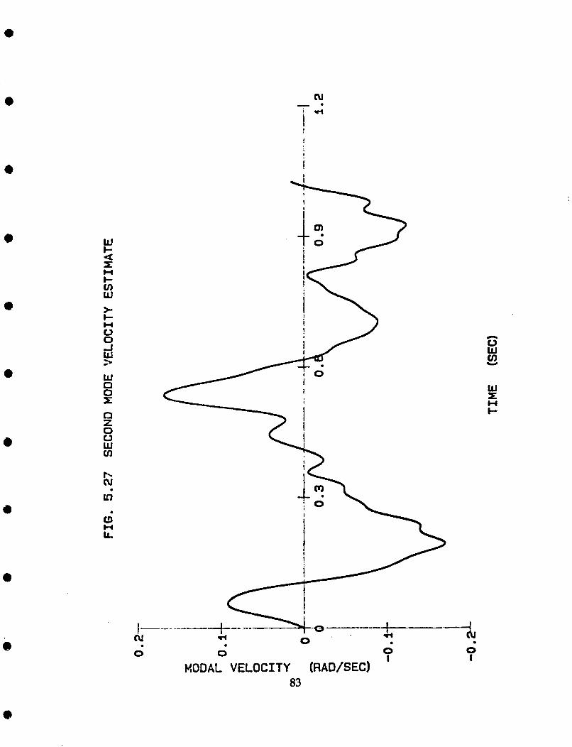
0

a Ji:

b (u

IC)

c3 H tL

. 0

I- N 0

0

1 i

\i !

n 0 W cn Y

W r H t-

T” !

i

I

t

I 1

‘-2

e

l-

U w a

Q) N

u)

Q H LL

. I \

h 0 w cn Y

W x H t-

a

c9 z H U P cn

e J

e

c 4: =E: H c v) W

l o

Q) N

NON-DIMENSIONAL SPRING COEFFICIENT 85

t z w H 0 H

a

0 m u) . a H lL

T:

i? 0

i I

i i I

1

I

I- >

*---.+-.+ P

I N I 9 tu 0

NON-DIKEtSIONAL DAKPING COEFFICIENT 86

H

0 LL

I- H n

I-

LL

a 0

0 0 0

NON-DIMENSIONAL PITCH FORCING COEFFICIENT 87

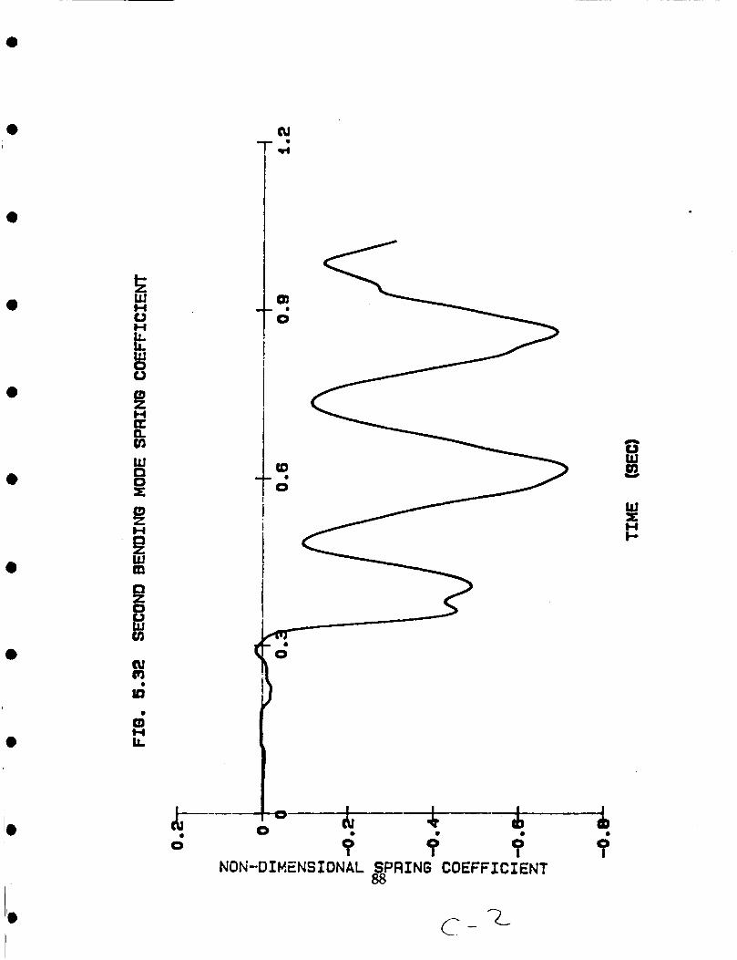
h E H

v1

1

i H Ir.

<

I I

-c) .h 7 + c--* + I 1 0 0 0

NON-DIHENSIONAL SPRING COEFFICIENT 88

x H I-

‘L C -

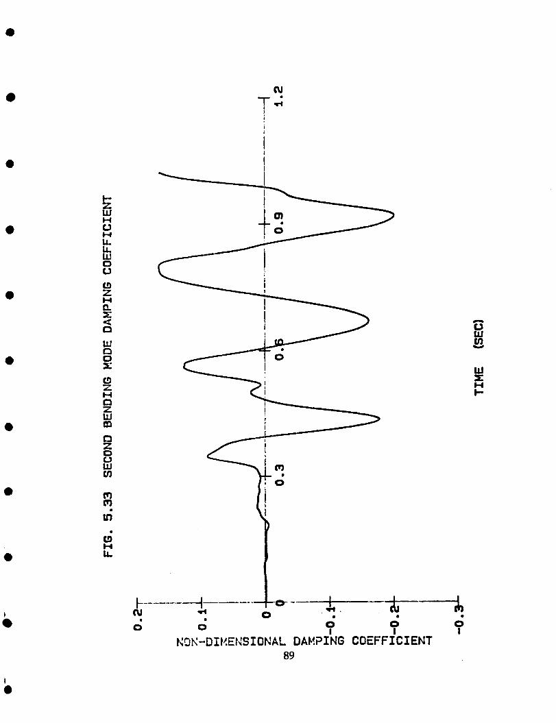
(u

TA i I I

I 0

0

0

e

e

c

a

1 k-- (u

0 a

I

RW-D I KEIZS IONAL D A W I ~ G COEFFICIE 89

NT

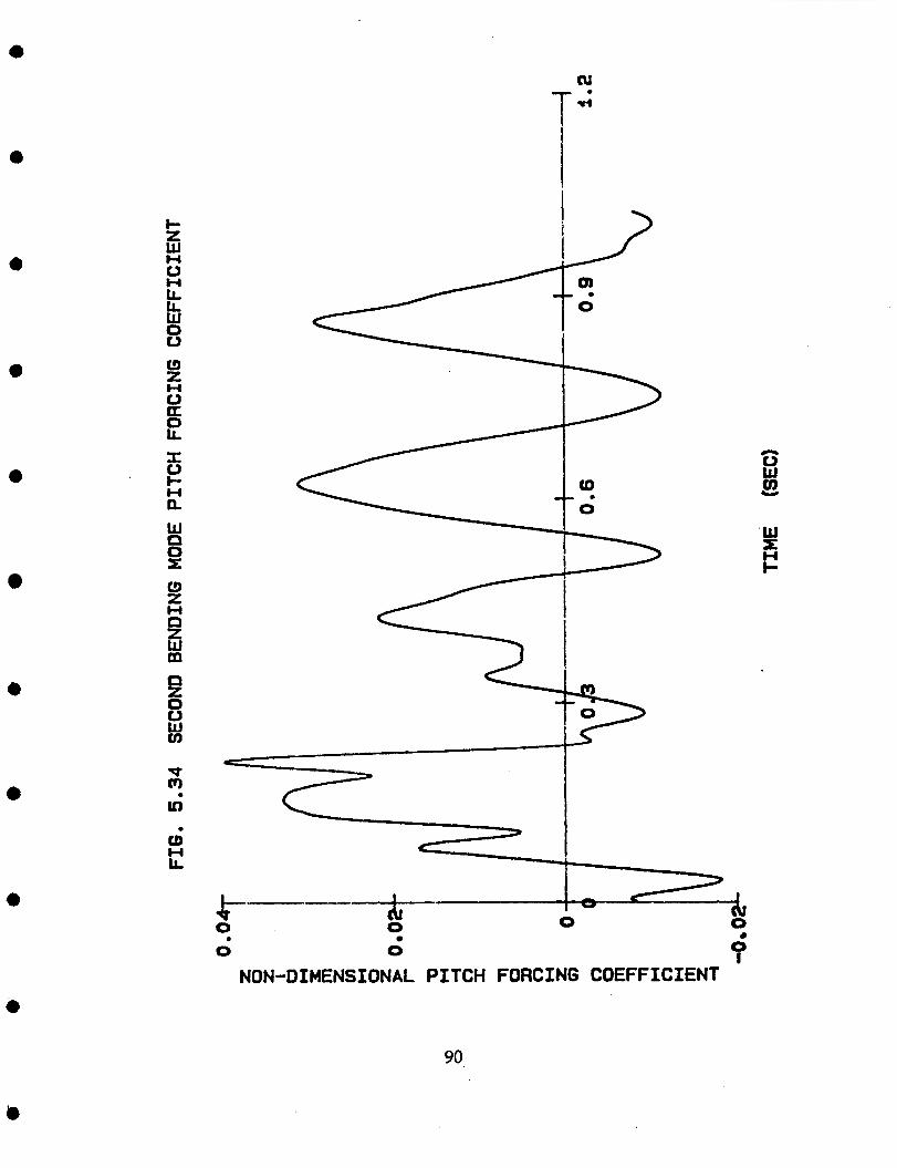
i- H e

k- -T 0 I 0 0 0

a

0 0 0 I

NON-DIMENSIONAL PITCH FORCING COEFFICIENT

90

References

a

e

a

6)

Fay, John, The Helicopter; history, piloting and how it flies, David &

Charles, Inc., North Pomfret, Vt, 1976.

Shaw, John, Albion, Nicholas, Hanker, Edward J. Jr, and Teal,

Richard S., Higher Harmonic Control: wind tunnel

demonstration of fully effective vibratory hub force suppression,

Journal of the AHS, January, 1989.

Johnson, Wayne, Helicopter Theory, Princeton University Press,

1980.

Bramwell, A. R. S., Helicopter Dynamics, Edward Arnold Ltd,

London, 91 76.

Putman, W., Curtiss, H. Jr., and Lapins, M., Low Speed Testing

Techniques for V/STOL Aircraft in the Princeton Dynamic Model

Track, Proc., AIAA 17th Aerospace Sciences Meeting, New Orleans,

La, January, 1979.

McKillip, Robert M. Jr., Active control rotor model testing at

Princeton's Rotorcraft Dynamics Laboratory, 2nd International

Conference on Rotorcraft Basic Research, University of Maryland, Md, February, 1988.

Demko, Michael G., High Speed Data Acquisition for the Princeton

University Dynamic Model Track, Master's Thesis, MAE

Department, Princeton University, Princeton, NJ, November, 1987.

McKillip, Robert M. Jr., Experimental Studies in System

Identification of Helicopter Rotor Dynamics, 14th European

Rotorcraft Forum, Milano, Italy, September, 1988.

Technical Manual, PDS-700-45, manual # M-4247, AYDIN VECTOR,

31 January, 1985.

91

e

e

e

e

e

Technical Manual, PAD-400-2, manual # M-4054, AYDIN VECTOR,

31 January, 1985. Hardy, Greg, Analysis and Design Methodology for Aeroelastic

Model Construction, Senior Independent Work, MAE Department,

Princeton University, Princeton, NJ, January, 1988. Halvorsen, William G., and Brown, David L., Impulse Technique

for Structural Frequency Response Testing, Cincinnati, Ohio.

Yntema, Robert T., Simplified Procedures and Charts for the rapid

Estimation of Bending Frequencies of Rotating Beams, National

Advisory Committee for Aeronautics Technical Note 3459, Langley

Aeronautical Laboratory, Langley Field, Va, June, 1955. Meirovitch, Leonard, Elements of Vibration Analysis, McGraw-Hill,

Inc., USA, 1986. McKillip, Robert M. Jr., Criteria for Determining the Spanwise

Position of Flatwise Accelerometers on the Blades of the NASA

Ames RTR Model Helicopter, January, 1987. McKillip, Robert M. Jr., Kinematic Observers for Active Control of Helicopter Rotor Vibration, Vertica, Volume 12, No. 1/2, pp. 1-11,

1988.

Moroney, M. J., Facts from Figures, Cox & Wyman Ltd., Landon, 1951.

Stengel, Robert F., Stochastic Optimal Control, John Wiley & Sons

Inc., 1986. Ham, N. D., Helicopter Blade Flutter, AGARD Report No. 607, January, 1973.

92

APPENDIX

93

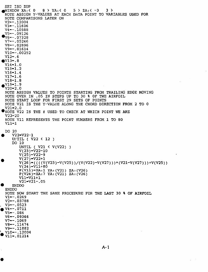
SET IS0 ZUP

NOTE ASSIGN Y-VALUES AT EACH DATA POINT TO VARIABLES USED FOR NOTE COMPARISONS LATER ON V2=-.12004 V3=-.11606 V4=-. 10588 V5--. 09126

.V6=-. 07328 V7=-.05246 V8--.02896 V9=-.01614 V10=-.00252

.WINDOW XA:< 0 8 > YA:< 0 5 > ZA:< -3 3 >

V12-. 6 .V13-. 8 V14-1.0 V15-1.2 V16-1.4 V17-1.6 V18-1.8

v20-2.0 NOTE ASS

*v19=1.9

GN iUES T INT ‘E! START NOTE OVER IN .05 IN STEPS UP TO 30

NG FROM TRAILING EDGE MOVI % OF THE AIRFOIL

NOTE START LOOP FOR FIRST 29 SETS OF POINTS

n J

NOTE V21 IS THE Y-VALUE ALONG THE CHORD DIRECTION FROM 2 TO 0 v21-2.0

v22=20 NOTE V11 REPRESENTS THE POINT NUMBERS FROM 1 TO 80 v11-1

*NOTE v22 IS THE # USED TO CHECK AT WHICH POINT WE ARE

DO 20 0 v22=v22-1

UI’TIL ( V22 < 12 ) DO 10

UNTIL ( V21 < V(V22) ) V(23)=V22-10 V(25)=V22-9 V(27)-V22+1 V(26)-((((V(V23)-V(V25))/(V(V22)-V(V27)))*(V2l-V(V27)))+V(V25)) V( 24)=V11+80 P(Vll)-XA:l YA:(V21) ZA:(V26) P(V24)=XA:7 YA:(V21) ZA:(V26) v11=v11+1 V21=V21-.05

a

0 EKDDO ENDDO NOTE NOW START THE SAME PROCEDURE FOR THE LAST 30 % OF AIRFOIL V1=-. 0249 V2=-,03788 . V3=-.0523 V4=-. 0711 V5=-. 004 V6=-.09366 V7--. 1069 V0=-. 11474 V9=-.11882 V10=-.12004 V11=. 01214

A- I

0

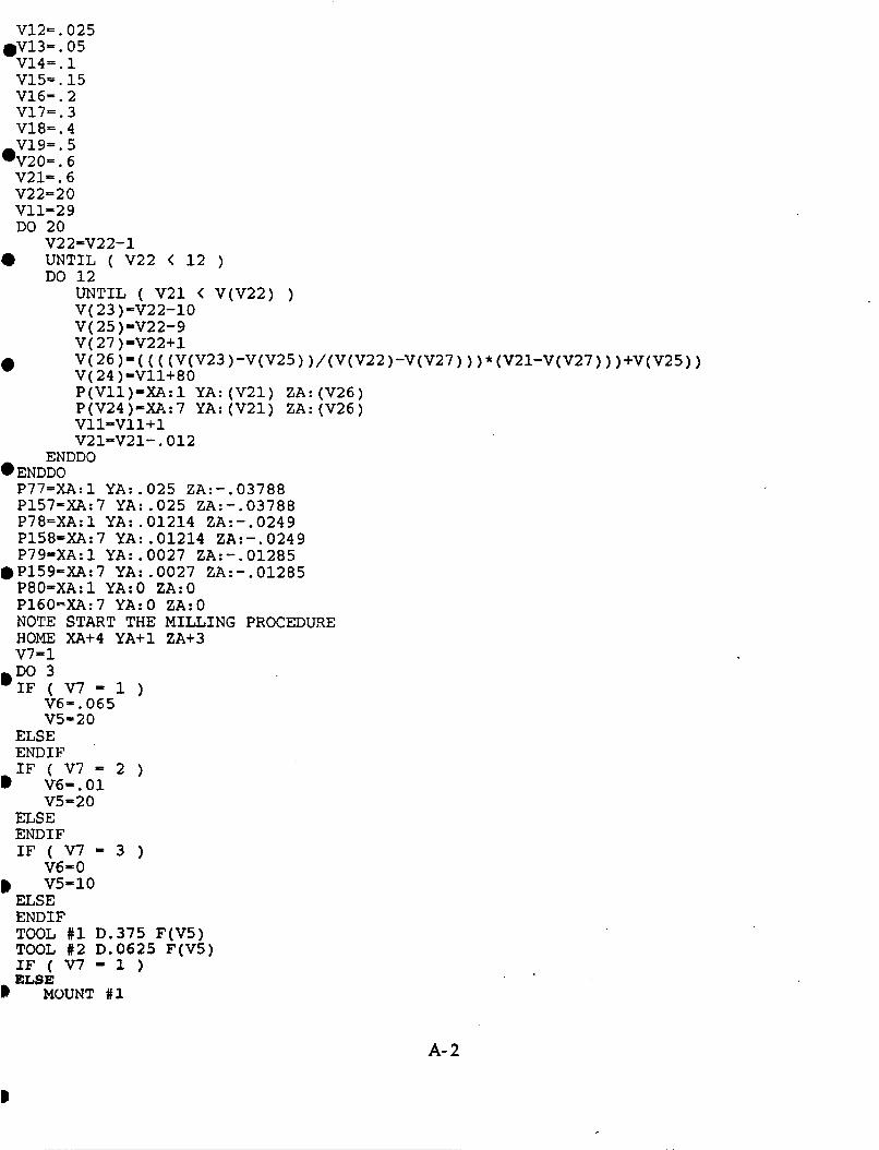
V12-. 025 aVl3-. 05 V14=. 1 V15=. 15 V16=. 2 V17-. 3 V18=. 4 v19=. 5

*V20-. 6 V21-. 6 v22-20 Vll-29 DO 20

v2 2-v22-1

DO 12 0 UNTIL ( V22 < 12 )

UNTIL ( V21 < V(V22) ) V( 23 )=V22-10 V(25)-V22-9 V(27)-V22+1 V(26)-((((V(V23)-V(V25))/(V(V22)-V(V27)))*(V2l-V(V27)))+V(V25)) V(24)=V11+80 P(Vll)=XA:l YA:(V21) ZA:(V26) P(V24)=XA:7 YA:(V21) ZA:(V26) Vll-V11+1 v21-v21-.012

0

ENDDO 0 ENDDO P77sXA:l YA:.025 ZA:-.03788 P157=XA:7 YA:.O25 ZA:-.03788 P78=XA:1 YA:.01214 ZA:-.0249 P158=XA:7 YA:.O1214 ZA:-.0249 P7gnXA:1 YAz.0027 ZA:-.01285

@P159=XA:7 YA:.OO27 ZA:-.01285 P80sXA:l YA:O ZA:O P160=XA:7 YA:O ZA:O NOTE START THE MILLING PROCEDURE HOME XA+4 YA+1 ZA+3 V7-1 DO 3

'IF ( V7 = 1 ) V6-. 065 V5-20

ELSE ENDIF IF ( V 7 - 2 )

@ V6=.01 V5-20

ELSE ENDIF IF ( V7 = 3 )

V6-0 V5-10

ELSE ENDIF TOOL #1 D.375 F(V5) TOOL #2 D.0625 F(V5) IF ( V7 = 1 ) ELSE

D MOUNT #1

A- 2

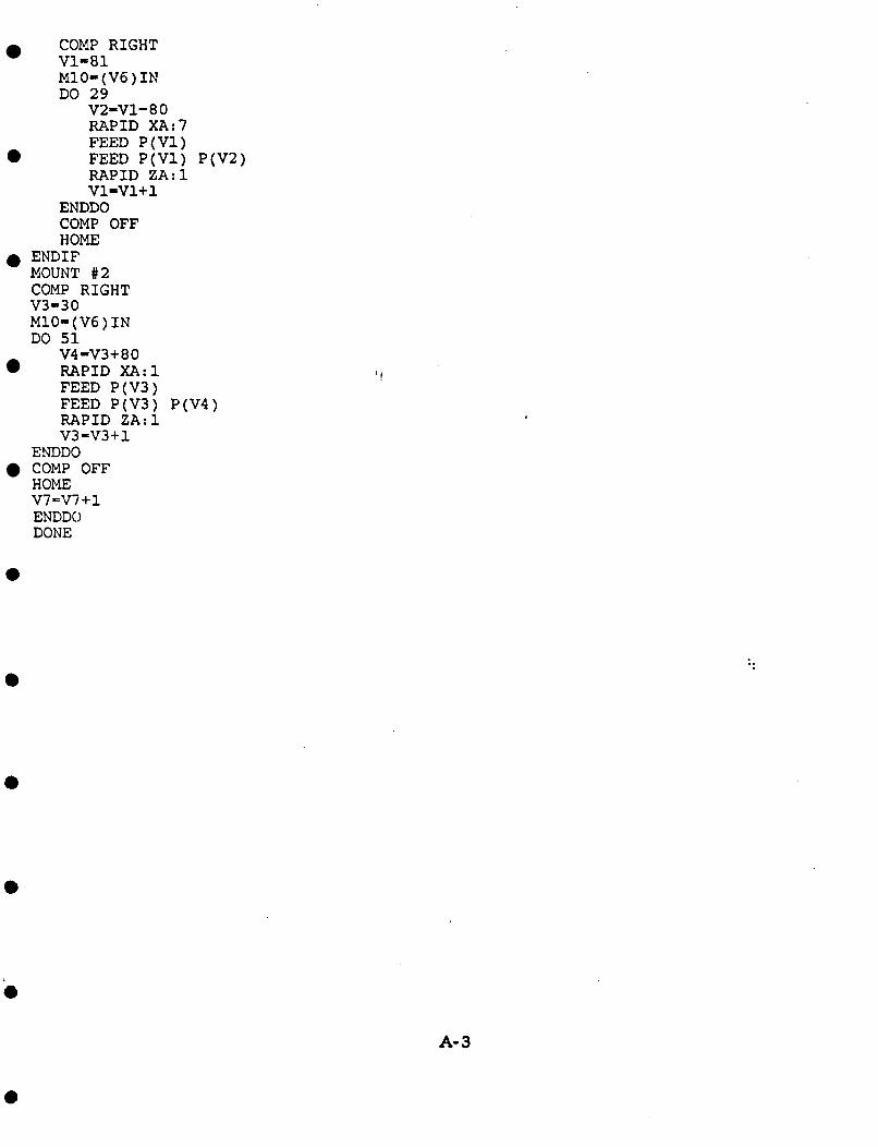
COMP RIGHT V1-81 M10-(V6)IN DO 29

V2-V1-80 RAPID XA:7 FEED P(V1)

0 FEED P(V1) P(V2) RAPID ZA:l Vl=V1+1

ENDDO COMP O F F HOME

0 ENDIF MOUNT #2 COMP RIGHT V3-30 M10=(V6)IN DO 51

V4 =V3+ 8 0 RAPID XA:1 FEED P(V3) FEED P(V3) P(V4) RAPID ZA:l V3-V3+1

ENDDO COMP O F F HOME V7-V7+1 ENDDO DONE

..

e

A- 3