Design of a Hybrid Genetic Algorithm for Parallel Machines ... · genetic algorithm for single-machine batch delivery scheduling problem with the objectives of minimizing the

Journal of Optimization in Industrial Engineering, Vol. 11, Issue 1,Winter and Spring 2018, 35-50 DOI:10.22094/JOIE.2018.272

35

Design of a Hybrid Genetic Algorithm for Parallel Machines Scheduling to Minimize Job Tardiness and Machine Deteriorating

Costs with Deteriorating Jobs in a Batched Delivery System

Mohammad Saidi-Mehrabada, Samira Bairamzadehb,*

a Professor, Department of Industrial Engineering, Iran University of Science and Technology, Tehran, Iran

b Ph.D. Student, Department of Industrial Engineering, Iran University of Science and Technology, Tehran, Iran Received17 July 2014; Revised 19 September 2015; Accepted 26 December 2016

Abstract This paper studies the parallel machine scheduling problem subject to machine and job deterioration in a batched delivery system. By the machine deterioration effect, we mean that each machine deteriorates over time, at a different rate. Moreover, job processing times are increasing functions of their starting times and follow a simple linear deterioration. The objective functions are minimizing total tardiness, delivery, holding and machine deteriorating costs. The problem of total tardiness on identical parallel machines is NP-hard, thus the under investigation problem, which is more complicated, is NP-hard too. In this study, a mixed-integer programming (MILP) model is presented and an efficient hybrid genetic algorithm (HGA) is proposed to solve the concerned problem. A new crossover and mutation operator and a heuristic algorithm have also been proposed depending on the type of problem. In order to evaluate the performance of the proposed model and solution procedure, a set of small to large test problems are generated and results are discussed. The related results show the effectiveness of the proposed model and GA for test problems.

Keywords: Parallel machine scheduling, Machine deterioration, Job deterioration, Batched delivery system, Genetic algorithm.

1. Introduction

Parallel machine scheduling as a very traditional branch of research studies have addresses from various aspects with an endeavor to minimize makespan, tardiness, completion time, waiting time, idle time and so on (Bandyopadhyay & Bhattacharya, 2013). In a real world application, the performance of each machine deteriorates over time at a random rate caused by processing the jobs. Moreover, while waiting for processing, jobs also may deteriorate. Deterioration of a job means that

a job processing time is

defined by a function of its starting times and positions in the sequence (Mazdeh et al., 2010). On the other hand, manufacturers aims at schedule their production activities such that be able to meet the due dates of their customers’ orders. The other issue accounted for in scheduling is the delivery costs of the jobs or Designing a batch of products, to be delivered. Batched delivery system means that the jobs of each customer could be delivered to it in one or many batches. Such a delivery system may leads to different completion and delivery/rendition times for

jobs. Although batched delivery system seems a reasonable approach in reducing transportation costs, but it may leads to increasing the number of tardy jobs or the total tardiness (Hamidinia et al., 2012; Karimi & Davoudpour, 2015). The problem of scheduling with the batch delivery system first introduced by Cheng and Kahlbacher (Cheng & Kahlbacher, 1993). They studied the single-machine batch delivery scheduling problem with the objective of minimizing the sum of earliness penalties, as well as delivery costs. Also, the authors proved that the problem is NP-hard in the ordinary sense but polynomially solvable for equal weights. In another study, Wang and Cheng (Wang & Cheng, 2000) considered a problem of parallel-machine batch delivery scheduling with the objective of minimizing the sum of flow times and delivery cost and showed that the problem is strongly NP-hard. They developed dynamic programming algorithm for the problem and presented two polynomial time algorithms in the cases that the job assignment is predetermined or the job processing times are all identical. *Corresponding author Email address:

[email protected]

Mohammad Saidi-Mehrabad et al. / Design of a Hybrid Genetic…

36

Hall and Potts (Hall & Potts, 2003) provided dynamic programming solutions for a range of scheduling problems with batched delivery systems in a supply chain with the aim of minimizing overall scheduling and delivery costs,cost, using several classical scheduling objectives. Mazdeh et al. (Mazdeh et al., 2007) proposed branch and bound algorithms for weighted sum of flow times in a batched delivery system, when all jobs are available at the time zero and in the presence of ready time. Mazdeh et al. (Mazdeh et al., 2011) developed a branch-and-bound algorithm for single machine batch delivery scheduling problem with the objective of minimising the sum of weighted flow times and delivery costs and with the assumption that the delivery cost is a linear increasing function of the number of deliveries. Hamidinia et al. (Hamidinia et al., 2012) suggested a genetic algorithm for single-machine batch delivery scheduling problem with the objectives of minimizing the sum of earliness, tardiness, holding, and delivery costs. Moreover, the authors presented a mathematical model for the problem.Yin et al. (Yin et al., 2014) addressed the problem of scheduling n nonresumable and simultaneously available jobs on a single machine in which the jobs were delivered in batches to the customers. They assumed a fixed unavailability interval for the machine during which the production is not allowed and along with a scheduling decision, a batching decision has to be determined so as to minimize the sum of total flow time and batch delivery cost, where the cost per batch delivery is fixed and independent of the number of jobs in the batch. They showed that the problem is NP-hard based on a reduction from the Equal-Size Partition Problem and presented a pseudo-polynomial time dynamic programming algorithm. Moreover, they developed a fully polynomial time approximation scheme (FPTAS) and a bicriteria fully polynomial time approximation scheme. Recently, Ahmadizar and Farhadi (Ahmadizar & Farhadi, 2015) addressed a single-machine batch delivery system scheduling problem to minimize the sum of earliness, tardiness, holding, and delivery costs in which jobs were released in different points in time. They presented a mathematical model and a set of dominance properties. In order to solve this NP-hard problem, they proposed a hybrid algorithm by integrating the dominance properties with an imperialist competitive algorithm. Karimi and Davoudpour (Karimi & Davoudpour, 2015) addressed the scheduling of supply chain with interrelated factories containing suppliers and manufacturers in which jobs transportation among factories and also delivery to the customer can be performed by batch of jobs. In order to

solve the problem, branch and bound algorithm was adopted and a lower bound and a standalone heuristic which was used as an upper bound were also introduced. On the other hand, Mazdeh et al. (Mazdeh et al., 2010) studied the problem of parallel machines scheduling to minimize job tardiness and machine deteriorating cost with deteriorating jobs and proposed LP-metric method to show the importance of their proposed multi-objective problem. It should be noted that the main difference of our study by Mazdeh et al. (Mazdeh et al., 2010) is that we consider batch delivery system for the same parallel machine scheduling while in Mazdeh et al. (Mazdeh et al., 2010) there is no assumption of batch scheduling problem. Moreover, in addition to machine deteriorating cost with deteriorating jobs which are addressed in both study, because of the inherent properties of the batch delivery scheduling problem, objectives of delay, holding (inventory) and delivery costs are added. Although batch scheduling problem have already been studied in a number of studies, but most of them have addressed the concerned problem in the case of single machine. Moreover, there is no existing study which proposes a mathematical model for the parallel machines batch delivery scheduling problem in the deteriorating environment. This paper aims at solving the problem of parallel machine scheduling to minimize total tardiness costs of deteriorating jobs plus their delivery costs and machine deteriorating costs in a batched delivery system when all jobs are available at time zero and preemption is not allowed. In order to solve the presented model, a hybrid genetic algorithm is proposed. To the best of our knowledge, there is not any paper that addresses the assumptions which are considered in this paper simultaneously. The rest of this paper is organized as follows: section 2 provides a review on the related literature. Section 2 defines the problem and presents the mathematical model for the problem. The proposed hybrid GA is developed in section 3, and finally Section 4 describes the computational results.

2. Problem description

2.1. Problem definition

There are N independent jobs has to be processed on m parallel machines. Machines can process all jobs in different speeds. The jobs belong to F customers while each of them has o(j) orders/jobs (1≤j≤F).The processing time of the ith job of the jth customer on machine m is given as a linear increasing function dependent on its starting time and a

Journal of Optimization in Industrial Engineering, Vol. 11, Issue 1,Winter and Spring 2018, 35-50

37

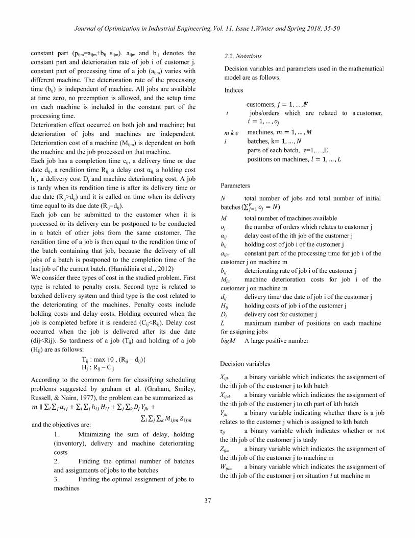
constant part (pijm=aijm+bij sijm). aijm and bij denotes the constant part and deterioration rate of job i of customer j. constant part of processing time of a job (aijm) varies with different machine. The deterioration rate of the processing time (bij) is independent of machine. All jobs are available at time zero, no preemption is allowed, and the setup time on each machine is included in the constant part of the processing time. Deterioration effect occurred on both job and machine; but deterioration of jobs and machines are independent. Deterioration cost of a machine (Mijm) is dependent on both the machine and the job processed on that machine. Each job has a completion time cij, a delivery time or due date dij, a rendition time Rij, a delay cost αij, a holding cost hij, a delivery cost Dj and machine deteriorating cost. A job is tardy when its rendition time is after its delivery time or due date (Rij>dij) and it is called on time when its delivery time equal to its due date (Rij=dij). Each job can be submitted to the customer when it is processed or its delivery can be postponed to be conducted in a batch of other jobs from the same customer. The rendition time of a job is then equal to the rendition time of the batch containing that job, because the delivery of all jobs of a batch is postponed to the completion time of the last job of the current batch. (Hamidinia et al., 2012) We consider three types of cost in the studied problem. First type is related to penalty costs. Second type is related to batched delivery system and third type is the cost related to the deteriorating of the machines. Penalty costs include holding costs and delay costs. Holding occurred when the job is completed before it is rendered (Cij<Rij). Delay cost occurred when the job is delivered after its due date (dij<Rij). So tardiness of a job (Tij) and holding of a job (Hij) are as follows:

Tij : max {0 , (Rij – dij)} Hj : Rij – Cij

According to the common form for classifying scheduling problems suggested by graham et al. (Graham, Smiley, Russell, & Nairn, 1977), the problem can be summarized as

1. Minimizing the sum of delay, holding (inventory), delivery and machine deteriorating costs 2. Finding the optimal number of batches and assignments of jobs to the batches 3. Finding the optimal assignment of jobs to machines

Decision variables

Xijk a binary variable which indicates the assignment of the ith job of the customer j to kth batch Xijek a binary variable which indicates the assignment of the ith job of the customer j to eth part of kth batch Yjk a binary variable indicating whether there is a job relates to the customer j which is assigned to kth batch τij a binary variable which indicates whether or not the ith job of the customer j is tardy Zijm a binary variable which indicates the assignment of the ith job of the customer j to machine m Wijlm a binary variable which indicates the assignment of the ith job of the customer j on situation l at machine m

2.2. Notations

Decision variables and parameters used in the mathematical model are as follows:

Indices

j i jobs/orders which are related to a customer,

m k e l

customers, 𝑗 = 1,… , 𝐹

𝑖 = 1,… , 𝑜𝑗

machines, 𝑚 = 1,… ,𝑀

batches, k= 1,… ,𝑁

parts of each batch, e=1,…,E

positions on machines, 𝑙 = 1,… , 𝐿

Parameters

N total number of jobs and total number of initial batches

M total number of machines available oj the number of orders which relates to customer j αij delay cost of the ith job of the customer j hij holding cost of job i of the customer j aijm constant part of the processing time for job i of the customer j on machine m bij deteriorating rate of job i of the customer j Mjm machine deterioration costs for job i of the customer j on machine m dij delivery time/ due date of job i of the customer j Hij holding costs of job i of the customer j Dj delivery cost for customer j L maximum number of positions on each machine for assigning jobs bigM A large positive number

(∑𝐹 𝑜𝑗 = 𝑁𝑗=1 )

and the objectives are:

푚 ∥ ∑ ∑ 훼 + ∑ ∑ ℎ 퐻 + ∑ ∑ 퐷 푌 +

∑ ∑ ∑ 푀 푍


38

Pijm processing time of the ith job of the customer j on machine m Sijm starting time of job i of the customer

j on machine

m

completion time of job i of the customer j

completion time of kth batch

Tij tardiness of job i of the customer j

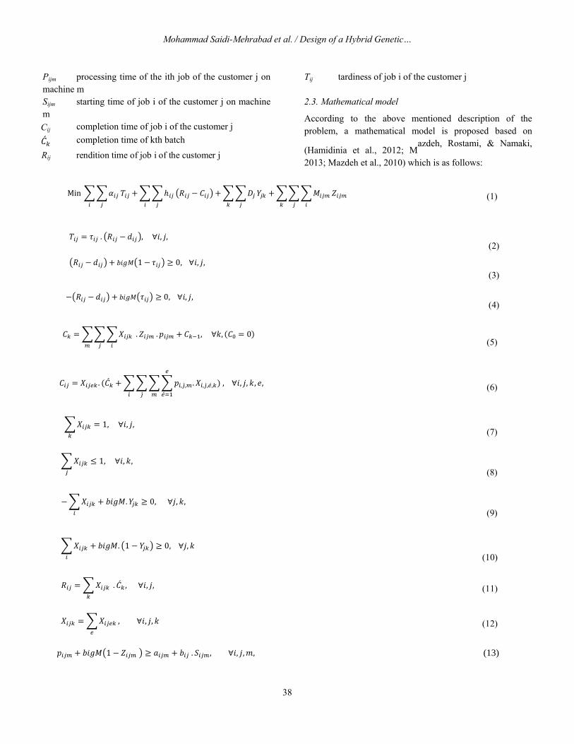
2.3. Mathematical model

According to the above mentioned description of the problem, a mathematical model is proposed based on

(Hamidinia et al., 2012; Mazdeh, Rostami, & Namaki,

2013; Mazdeh et al., 2010) which is as follows:

(1)

(2)

(3)

(4)

(5)

(6)

(7)

(8)

(9)

(10)

(11)

(12)

Min 훼 푇 + ℎ 푅 − 퐶 + 퐷 푌 + 푀 푍

푇 = 휏 . 푅 − 푑 , ∀푖, 푗,

푅 − 푑 + 푏푖푔푀 1 − 휏 ≥ 0, ∀푖, 푗,

− 푅 − 푑 + 푏푖푔푀 휏 ≥ 0, ∀푖, 푗,

퐶 = 푋 . 푍 . 푝 + 퐶 , ∀푘, (퐶 = 0)

𝐶𝑖𝑗 = 𝑋𝑖𝑗𝑒𝑘. (�́�𝑘 + ∑∑∑∑𝑝�́�,�́�,𝑚. 𝑋�́�,�́�,�́�,𝑘

𝑒

�́�=1𝑚�́��́�

) , ∀𝑖, 𝑗, 𝑘, 𝑒,

∑𝑋𝑖𝑗𝑘

𝑘

= 1, ∀𝑖, 𝑗,

∑𝑋𝑖𝑗𝑘

𝑗

≤ 1, ∀𝑖, 𝑘,

−∑𝑋𝑖𝑗𝑘

𝑖

+ 𝑏𝑖𝑔𝑀.𝑌𝑗𝑘 ≥ 0, ∀𝑗, 𝑘,

∑𝑋𝑖𝑗𝑘

𝑖

+ 𝑏𝑖𝑔𝑀. (1 − 𝑌𝑗𝑘) ≥ 0, ∀𝑗, 𝑘

𝑅𝑖𝑗 = ∑𝑋𝑖𝑗𝑘

𝑘

. �́�𝑘, ∀𝑖, 𝑗,

𝑋𝑖𝑗𝑘 = ∑𝑋𝑖𝑗𝑒𝑘

𝑒

, ∀𝑖, 𝑗, 𝑘

𝑝𝑖𝑗𝑚 + 𝑏𝑖𝑔𝑀(1 − 𝑍𝑖𝑗𝑚 ) ≥ 𝑎𝑖𝑗𝑚 + 𝑏𝑖𝑗 . 𝑆𝑖𝑗𝑚, ∀𝑖, 𝑗,𝑚, (13)

Cij

�́�𝑘

Rij rendition time of job i of the customer j

39

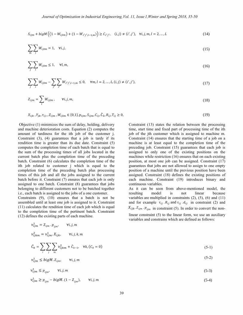
Objective (1) minimizes the sum of delay, holding, delivery and machine deterioration costs. Equation (2) computes the amount of tardiness for the ith job of the customer j. Constraint (3), (4) guarantees that a job is tardy if its rendition time is greater than its due date. Constraint (5) computes the completion time of each batch that is equal to the sum of the processing times of all jobs located in the current batch plus the completion time of the preceding batch. Constraint (6) calculates the completion time of the ith job related to customer j which is equal to the completion time of the preceding batch plus processing times of this job and all the jobs assigned to the current batch before it. Constraint (7) ensures that each job is only assigned to one batch. Constraint (8) guarantees that jobs belonging to different customers not to be batched together i.e., each batch is assigned to the jobs of a one customer. Constraints (9), (10) ensures that a batch is not be assembled until at least one job is assigned to it. Constraint (11) calculates the rendition time of each job which is equal to the completion time of the pertinent batch. Constraint (12) defines the existing parts of each machine.

Constraint (13) states the relation between the processing time, start time and fixed part of processing time of the ith job of the jth customer which is assigned to machine m. Constraint (14) ensures that the starting time of a job on a machine is at least equal to the completion time of the preceding job. Constraint (15) guarantees that each job is assigned to only one of the existing positions on the machines while restriction (16) ensures that on each existing position, at most one job can be assigned. Constraint (17) guarantees that jobs are not allowed to assign to one empty position of a machine until the previous position have been assigned. Constraint (18) defines the existing positions of each machine. Constraint (19) introduces binary and continuous variables. As it can be seen from above-mentioned model, the resulting model is not linear because variables are multiplied in constraints (2), (5), (6) and (11) and for example in constraint (2) and

in constraint (5). In order to convert the non-

linear constraint (5) to the linear form, we use an auxiliary variables and constrains which are defined as follows:

(5-1)

(5-2)

𝑆𝑖𝑗𝑚 + 𝑏𝑖𝑔𝑀 ((1 − 𝑊𝑖𝑗𝑙𝑚) + (1 − 𝑊𝑖′𝑗′,𝑙−1,𝑚)) ≥ 𝐶𝑖′𝑗′, (𝑖, 𝑗) ≠ (𝑖′, 𝑗′), ∀𝑖, 𝑗, 𝑚, 𝑙 = 2,… , 𝐿 (14)

∑∑𝑊𝑖𝑗𝑙𝑚

𝑙𝑚

= 1, ∀𝑖, 𝑗, (15)


𝑖𝑗

≤ 1, ∀𝑙,𝑚, (16)


𝑖𝑗

− ∑∑𝑊𝑖′𝑗′,𝑙−1,𝑚

𝑖′𝑗′

≤ 0, ∀𝑚, 𝑙 = 2,… , 𝐿, (𝑖, 𝑗) ≠ (𝑖′, 𝑗′), (17)

𝑍𝑖𝑗𝑚 = ∑𝑊𝑖𝑗𝑙𝑚

𝑙

, ∀𝑖, 𝑗, 𝑚, (18)

𝑋𝑖𝑗𝑘 , 𝑌𝑗𝑘, 𝜏𝑖𝑗, , 𝑍𝑖𝑗𝑚 ,𝑊𝑖𝑗𝑙𝑚 ∈ {0,1}, 𝑝𝑖𝑗𝑚, 𝑆𝑖𝑗𝑚, 𝐶𝑖𝑗, �́�𝑘, 𝑅𝑖𝑗, 𝑇𝑖𝑗 ≥ 0, (19)

𝜈𝑖𝑗𝑚1 = 𝑍𝑖𝑗𝑚 . 𝑝

𝑖𝑗𝑚, ∀𝑖, 𝑗, 𝑚

𝜈𝑖𝑗𝑘𝑚2 = 𝜈𝑖𝑗𝑚

1 . 𝑋𝑖𝑗𝑘, ∀𝑖, 𝑗, 𝑘, 𝑚

�́�𝑘 = ∑∑∑𝜈𝑖𝑗𝑘𝑚2

𝑚𝑗𝑖

+ �́�𝑘−1, ∀𝑘, (𝐶0 = 0)

𝜈𝑖𝑗𝑚1 ≤ 𝑏𝑖𝑔𝑀. 𝑍𝑖𝑗𝑚, ∀𝑖, 𝑗, 𝑚

𝜈𝑖𝑗𝑚1 ≤ 𝑝

𝑖𝑗𝑚, ∀𝑖, 𝑗, 𝑚 (5-3)

𝜈𝑖𝑗𝑚1 ≥ 𝑝

𝑖𝑗𝑚− 𝑏𝑖𝑔𝑀. (1 − 𝑍

𝑖𝑗𝑚), ∀𝑖, 𝑗, 𝑚 (5-4)

𝑋𝑖𝑗𝑘. 𝑍𝑖𝑗𝑚 . 𝑝𝑖𝑗𝑚

𝜏𝑖𝑗 . 𝑅𝑖𝑗 and 𝜏𝑖𝑗 . 𝑑𝑖𝑗



40

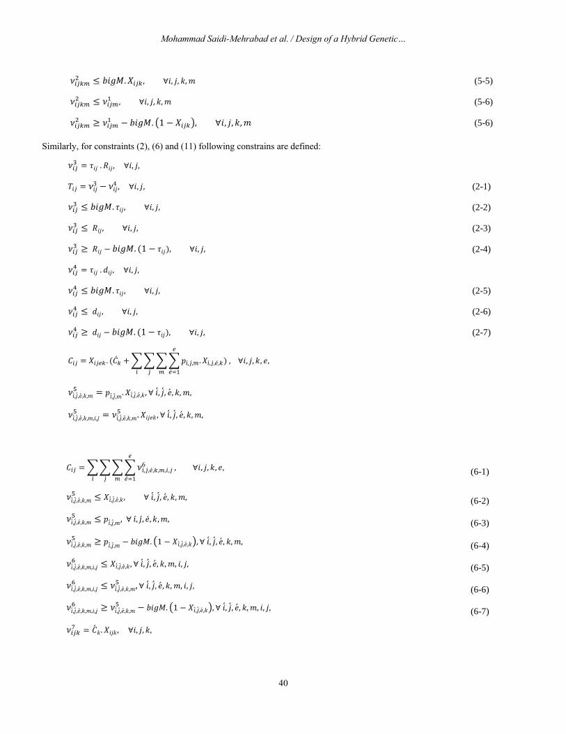
Similarly, for constraints (2), (6) and (11) following constrains are defined:

𝜈𝑖𝑗𝑘𝑚2 ≤ 𝑏𝑖𝑔𝑀. 𝑋𝑖𝑗𝑘 , ∀𝑖, 𝑗, 𝑘, 𝑚 (5-5)

𝜈𝑖𝑗𝑘𝑚2 ≤ 𝜈𝑖𝑗𝑚

1 , ∀𝑖, 𝑗, 𝑘, 𝑚 (5-6)

𝜈𝑖𝑗𝑘𝑚2 ≥ 𝜈𝑖𝑗𝑚

1 − 𝑏𝑖𝑔𝑀. (1 − 𝑋𝑖𝑗𝑘), ∀𝑖, 𝑗, 𝑘,𝑚 (5-6)

𝜈𝑖𝑗3 = 𝜏𝑖𝑗 . 𝑅𝑖𝑗, ∀𝑖, 𝑗,

𝑇𝑖𝑗 = 𝜈𝑖𝑗3 − 𝜈𝑖𝑗

4 , ∀𝑖, 𝑗, (2-1)

𝜈𝑖𝑗3 ≤ 𝑏𝑖𝑔𝑀. 𝜏𝑖𝑗, ∀𝑖, 𝑗, (2-2)

𝜈𝑖𝑗3 ≤ 𝑅𝑖𝑗, ∀𝑖, 𝑗, (2-3)

𝜈𝑖𝑗3 ≥ 𝑅𝑖𝑗 − 𝑏𝑖𝑔𝑀. (1 − 𝜏𝑖𝑗), ∀𝑖, 𝑗, (2-4)

𝜈𝑖𝑗4 = 𝜏𝑖𝑗 . 𝑑𝑖𝑗, ∀𝑖, 𝑗,

𝜈𝑖𝑗4 ≤ 𝑏𝑖𝑔𝑀. 𝜏𝑖𝑗, ∀𝑖, 𝑗, (2-5)

𝜈𝑖𝑗4 ≤ 𝑑𝑖𝑗 , ∀𝑖, 𝑗, (2-6)

𝜈𝑖𝑗4 ≥ 𝑑𝑖𝑗 − 𝑏𝑖𝑔𝑀. (1 − 𝜏𝑖𝑗), ∀𝑖, 𝑗, (2-7)

𝐶𝑖𝑗 = 𝑋𝑖𝑗𝑒𝑘 . (�́�𝑘 + ∑∑∑∑𝑝�́�,�́�,𝑚. 𝑋�́�,�́�,�́�,𝑘

𝑒

�́�=1𝑚�́��́�

) , ∀𝑖, 𝑗, 𝑘, 𝑒,

𝜈�́�,�́�,�́�,𝑘,𝑚5 = 𝑝

�́�,�́�,𝑚. 𝑋�́�,�́�,�́�,𝑘, ∀ �́�, �́�, �́�, 𝑘, 𝑚,

𝜈�́�,�́�,�́�,𝑘,𝑚,𝑖,𝑗5 = 𝜈�́�,�́�,�́�,𝑘,𝑚

5 .𝑋𝑖𝑗𝑒𝑘 , ∀ �́�, �́�, �́�, 𝑘, 𝑚,

𝐶𝑖𝑗 = ∑∑∑∑ 𝜈�́�,�́�,�́�,𝑘,𝑚,𝑖,𝑗6

𝑒

�́�=1𝑚�́��́�

, ∀𝑖, 𝑗, 𝑘, 𝑒,(6-1)

𝜈�́�,�́�,�́�,𝑘,𝑚5 ≤ 𝑋�́�,�́�,�́�,𝑘, ∀ �́�, �́�, �́�, 𝑘, 𝑚, (6-2)

𝜈�́�,�́�,�́�,𝑘,𝑚5 ≤ 𝑝

�́�,�́�,𝑚, ∀ �́�, �́�, �́�, 𝑘,𝑚,

(6-3)

𝜈�́�,�́�,�́�,𝑘,𝑚5 ≥ 𝑝

�́�,�́�,𝑚− 𝑏𝑖𝑔𝑀. (1 − 𝑋�́�,�́�,�́�,𝑘), ∀ �́�, �́�, �́�, 𝑘, 𝑚,

(6-4)

𝜈�́�,�́�,�́�,𝑘,𝑚,𝑖,𝑗6 ≤ 𝑋�́�,�́�,�́�,𝑘, ∀ �́�, �́�, �́�, 𝑘, 𝑚, 𝑖, 𝑗, (6-5)

𝜈�́�,�́�,�́�,𝑘,𝑚,𝑖,𝑗6 ≤ 𝜈�́�,�́�,�́�,𝑘,𝑚

5 ,∀ �́�, �́�, �́�, 𝑘, 𝑚, 𝑖, 𝑗, (6-6)

𝜈�́�,�́�,�́�,𝑘,𝑚,𝑖,𝑗6 ≥ 𝜈�́�,�́�,�́�,𝑘,𝑚

5 − 𝑏𝑖𝑔𝑀. (1 − 𝑋�́�,�́�,�́�,𝑘), ∀ �́�, �́�, �́�, 𝑘, 𝑚, 𝑖, 𝑗, (6-7)

𝜈𝑖𝑗𝑘7 = �́�𝑘. 𝑋𝑖𝑗𝑘, ∀𝑖, 𝑗, 𝑘,

41

By replacing constraints (2), (5), (6) and (11) with above mentioned numbered constraints the non-linear model is converted to an equivalent MILP model.

3. GA Implementation

Evolutionary algorithms (EAS) are the most studied population based metaheuristics which are applied to many real and complex problems (Talbi, 2009). GA is a very popular class of EAs which is inspired by the natural evolution of the living organisms. The basic concepts of GA have been described by the investigation studied by John Holland in the 1970s and Davis was first that proposes GA for solving scheduling problems (Davis & Coombs, 1987). A generic GA starts by creating an initial population of

chromosomes (solutions) and iteratively replaces the current population by a new population. Each chromosome/individual encodes a solution of the prob-lem, and its fitness value represents a measure of the quality of solution for the problem. In order to search potential better solutions, during each iteration (generation) genetic operators that are, crossover, mutation and natural selection are applied. Crossover operator creates new individuals by combining parts of two individuals while mutation operator creates new individuals, by a small change in a single individual. The following subsections present the components of the hybrid GA applied to solve the proposed model.

3.1. Solution representation

The initial and most important step in the GA is toconsider a chromosome structure or solution representation.

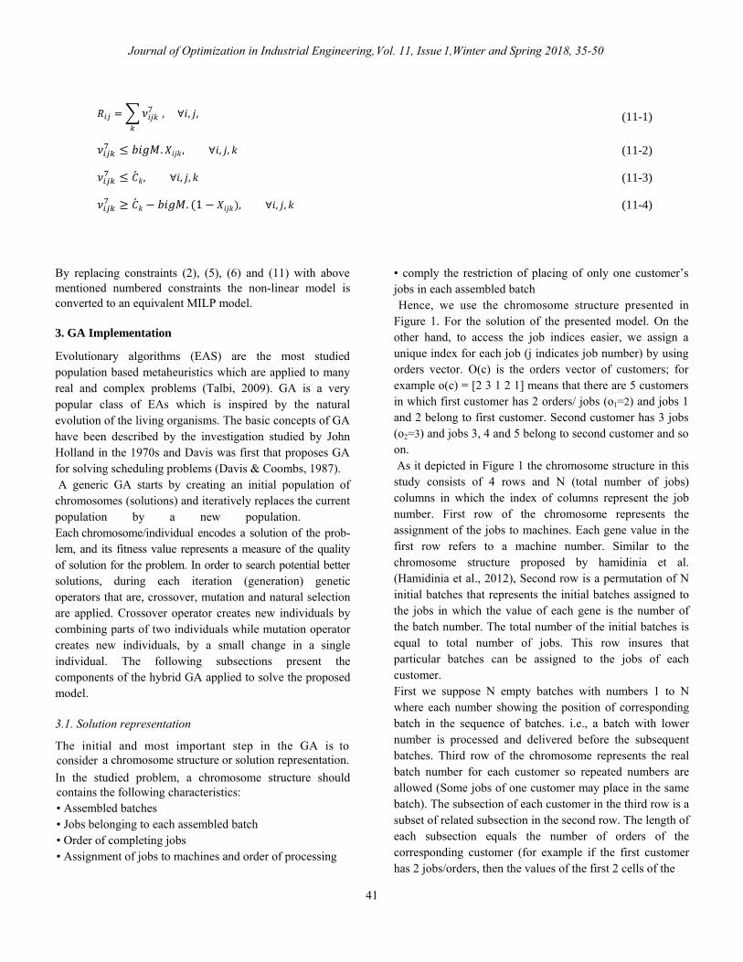
In the studied problem, a chromosome structure should contains the following characteristics: • Assembled batches • Jobs belonging to each assembled batch • Order of completing jobs • Assignment of jobs to machines and order of processing

• comply the restriction of placing of only one customer’s jobs in each assembled batch Hence, we use the chromosome structure presented in Figure 1. For the solution of the presented model. On the other hand, to access the job indices easier, we assign a unique index for each job (j indicates job number) by using orders vector. O(c) is the orders vector of customers; for example o(c) = [2 3 1 2 1] means that there are 5 customers in which first customer has 2 orders/ jobs (o1=2) and jobs 1 and 2 belong to first customer. Second customer has 3 jobs (o2=3) and jobs 3, 4 and 5 belong to second customer and so on. As it depicted in Figure 1 the chromosome structure in this study consists of 4 rows and N (total number of jobs) columns in which the index of columns represent the job number. First row of the chromosome represents the assignment of the jobs to machines. Each gene value in the first row refers to a machine number. Similar to the chromosome structure proposed by hamidinia et al. (Hamidinia et al., 2012), Second row is a permutation of N initial batches that represents the initial batches assigned to the jobs in which the value of each gene is the number of the batch number. The total number of the initial batches is equal to total number of jobs. This row insures that particular batches can be assigned to the jobs of each customer. First we suppose N empty batches with numbers 1 to N where each number showing the position of corresponding batch in the sequence of batches. i.e., a batch with lower number is processed and delivered before the subsequent batches. Third row of the chromosome represents the real batch number for each customer so repeated numbers are allowed (Some jobs of one customer may place in the same batch). The subsection of each customer in the third row is a subset of related subsection in the second row. The length of each subsection equals the number of orders of the corresponding customer (for example if the first customer has 2 jobs/orders, then the values of the first 2 cells of the

𝑅𝑖𝑗 = ∑𝜈𝑖𝑗𝑘7

𝑘

, ∀𝑖, 𝑗, (11-1)

𝜈𝑖𝑗𝑘7 ≤ 𝑏𝑖𝑔𝑀. 𝑋𝑖𝑗𝑘, ∀𝑖, 𝑗, 𝑘 (11-2)

𝜈𝑖𝑗𝑘7 ≤ �́�𝑘, ∀𝑖, 𝑗, 𝑘 (11-3)

𝜈𝑖𝑗𝑘7 ≥ �́�𝑘 − 𝑏𝑖𝑔𝑀. (1 − 𝑋𝑖𝑗𝑘), ∀𝑖, 𝑗, 𝑘 (11-4)



42

initial batches row could be used for packing this customer’s orders). The 4th row of the proposed chromosome is order priority row that consists of subsections of customer. Each subsection of the order priority row is a permutation of numbers between 1 and the length of the subsection, i.e.,

values in each subsection represents the processing order of related customer’s jobs. If some orders of a one customer place in different batches, the processing order of them are based on priority of their batches (according to batch numbers), but if these orders fall in the same batch the priority order specify the order of processing.

Job number: 1 2 O1 O1+1 O1+ O2 N- OF+1 N-1 N

Machine : … … … …

Initial batches:

Batch number:

Order priority:

First customer’s section

length= O1

Second customer’s section length= O2

Last customer’s section length= OF

Fig 1. Proposed chromosome structure

3.2. Chromosome decoding and fitness function

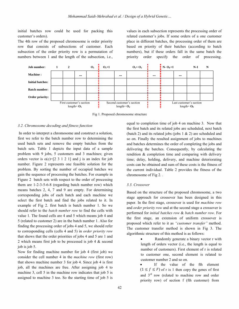
In order to interpret a chromosome and construct a solution, first we refer to the batch number row to determining the used batch sets and remove the empty batches from the batch sets. Table 1 depicts the input data of a sample problem with 9 jobs, 5 customers and 3 machines; given orders vector is o(c)=[2 3 1 2 1] and j is an index for job number. Figure 2 represents one feasible solution for the problem. By sorting the number of occupied batches we gain the sequence of processing the batches. For example in Figure 2 batch sets with respect to the order of processing them are 1-2-3-5-6-8 (regarding batch number row) which means batches 2, 4, 7 and 9 are empty. For determining corresponding jobs of each batch and each machine we select the first batch and find the jobs related to it. In example of Fig 2. first batch is batch number 1. So we should refer to the batch number row to find the cells with value 1. The found cells are 4 and 5 which means job 4 and 5 (related to customer 2) are in the batch number 1. Also for finding the processing order of jobs 4 and 5, we should refer to corresponding cells (cells 4 and 5) in order priority row that shows that the order priorities of jobs 4 and 5 are 1 and 2 which means first job to be processed is job 4 & second job is job 5.

Now for finding machine number for job 4 (first job) we consider the cell number 4 in the machine row (first row) that shows machine number 3 for job 4. Since job 4 is first job, all the machines are free. After assigning job 4 to machine 3, cell 5 in the machine row indicates that job 5 is assigned to machine 3 too. So the starting time of job 5 is

equal to completion time of job 4 on machine 3. Now that the first batch and its related jobs are scheduled, next batch (batch 2) and its related jobs (jobs 1 & 2) are scheduled and so on. Finally the resulted assignment of jobs to machines and batches determines the order of completing the jobs and delivering the batches. Consequently, by calculating the rendition & completion time and comparing with delivery time; delay, holding, delivery, and machine deteriorating costs can be obtained and sum of these costs is the fitness of the current individual. Table 2 provides the fitness of the chromosome of Fig 2. .

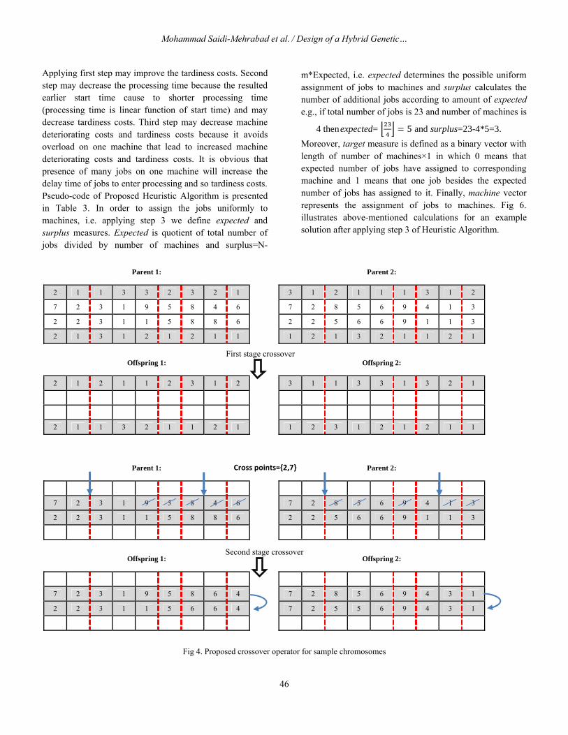
3.3. Crossover

Based on the structure of the proposed chromosome, a two stage approach for crossover has been designed in this paper. In the first stage, crossover is used for machine row

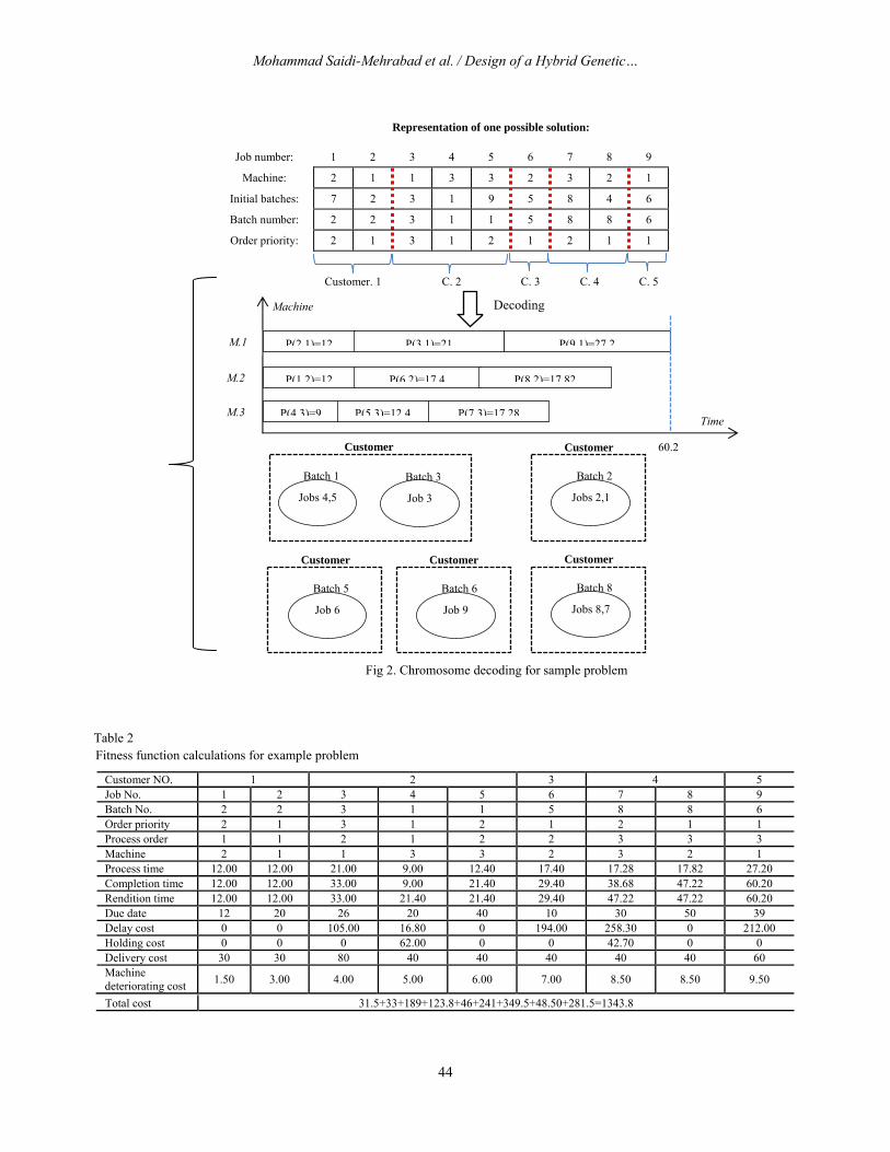
and order priority row and at the second stage a crossover is performed for initial batches row & batch number row. For the first stage, an extension of uniform crossover is proposed which refer to it as “customer transfer” method. The customer transfer method is shown in Fig 3. The algorithmic structure of this method is as follows:

Randomly generate a binary vector r with length of orders vector (i.e., the length is equal to number of customers). First element of r is related to customer one, second element is related to customer number 2 and so on. If the value of the fth element

of r is 1 then copy the genes of first and 3rd row (related to machine row and order priority row) of section f (fth customer) from

(1 ≤ 𝑓 ≤ 𝐹)

43

For applying crossover in the second stage for initial batches row and batch number row, first we use order

crossover (OX) on the initial batches row and then in order to preserve the feasibility of the solution, generate the new batch number row of the resulted offsprings from initial batches row. Order crossover can be summarizes as follows: First, two crossover points are randomly selected. From parent 1, one will copy in the offspring, at the same absolute positions, the part between the two points. From parent 2, one will start at the second crossover point and pick the elements that are not already selected from parent 1 to fill them in the offspring from the second crossover point. (Talbi, 2009) Crossover stages for the solutions of Fig 3 is illustrated in Fig 4.

Table 1 Input data for example problem

Number of jobs=9; number of customers=5; number of machines=3; o(c)=[2 3 1 2 1] Customer NO. 1 2 3 4 5 Job No. 1 2 3 4 5 6 7 8 9

Delivery time 12 20 26 20 40 10 30 50 39 Delay cost 10 15 15 12 13 10 15 12 10 Holding cost 5 5 5 5 5 Delivery cost 60 80 40 80 60

fixed part of the processing time(ajm) and growth rate of the processing time(bj) Job No. 1 2 3 4 5 6 7 8 9 Machine 1 10 12 15 5 9 10 12 12 14 Machine 2 12 8 16 7 6 9 10 9 12 Machine 3 14 14 12 9 7 9 13 8 16 bj 0.35 0.25 0.50 0.25 0.60 0.70 0.20 0.30 0.40 machines deteriorating cost (Mjm) Job No. 1 2 3 4 5 6 7 8 9 Machine 1 2 3 4 4 5 6.5 8 9 9.5 Machine 2 1.5 3 4.5 4.5 5.5 7 8 8.5 9 Machine 3 2.5 3.5 5 5 6 7.5 8.5 9.5 10

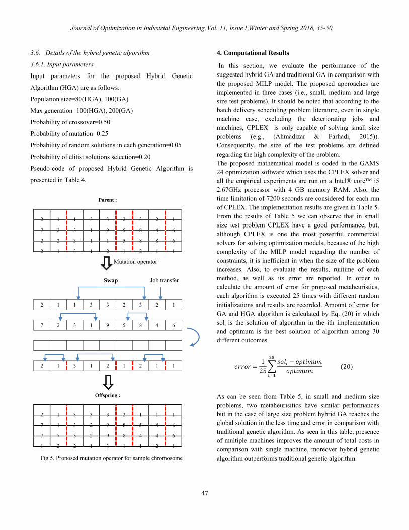
3.4. Mutation

In this study we utilize a mutation operator for machine row, initial batches and priority order rows.

3.4.1. Mutation operator for machine row

In this paper, two types of mutation is performed on the machine row. First type is called “job transfer” in which we select a random gene in the machine row (machine number) and change the value of it to another possible value from the machine set. This operation is equivalent to transfer one job from current machine to another machine. Second type is

swap mutation operator in which the value of two randomly selected genes is replaced. Number of mutation operation is performed (i.e., n(m)) in the machine row is dynamic and dependent on length of a chromosome and number of machines:

If n(m) is even, number of “job transfer” and swap processes are equal. And if n(m) is odd, number of swap operations is one unit more than “job transfer” operations. For the sample problem of Fig 2. n(m) is equal to 2 which means that one “job transfer” and one swap move is performed.

parent 1 to the corresponding locations of offspring 1 and copy the genes of first and 3rd row of section f from parent 2 to the corresponding locations of offspring 2. If the value of the fth element

of r is 0 then copy the genes of first and 3rd row of section f (fth customer) from parent 2 to the corresponding locations of offspring 1 and copy the genes of first and 3rd row of section f from

(1 ≤ 𝑓 ≤ 𝐹)

parent 1 to the corresponding locations of offspring 2.

𝑛 (𝑚) = [𝑡𝑜𝑡𝑎𝑙 𝑛𝑢𝑚𝑏𝑒𝑟 𝑜𝑓 𝑗𝑜𝑏𝑠

𝑛𝑢𝑚𝑏𝑒𝑟 𝑚𝑎𝑐ℎ𝑖𝑛𝑒𝑠] − 1 (19)



44

Fig 2. Chromosome decoding for sample problem

Table 2

Fitness function calculations for example problem

Customer NO. 1 2 3 4 5 Job No. 1 2 3 4 5 6 7 8 9 Batch No. 2 2 3 1 1 5 8 8 6 Order priority 2 1 3 1 2 1 2 1 1 Process order 1 1 2 1 2 2 3 3 3 Machine 2 1 1 3 3 2 3 2 1 Process time 12.00 12.00 21.00 9.00 12.40 17.40 17.28 17.82 27.20 Completion time 12.00 12.00 33.00 9.00 21.40 29.40 38.68 47.22 60.20 Rendition time 12.00 12.00 33.00 21.40 21.40 29.40 47.22 47.22 60.20 Due date 12 20 26 20 40 10 30 50 39 Delay cost 0 0 105.00 16.80 0 194.00 258.30 0 212.00 Holding cost 0 0 0 62.00 0 0 42.70 0 0 Delivery cost 30 30 80 40 40 40 40 40 60 Machine deteriorating cost

1.50 3.00 4.00 5.00 6.00 7.00 8.50 8.50 9.50

Representation of one possible solution:

Job number: 1 2 3 4 5 6 7 8 9

Machine: 2 1 1 3 3 2 3 2 1

Initial batches: 7 2 3 1 9 5 8 4 6

Batch number: 2 2 3 1 1 5 8 8 6

Order priority: 2 1 3 1 2 1 2 1 1

Customer. 1

C. 2

C. 3

C. 4

C. 5

DecodingMachine

Time

P(2,1)=12 P(3,1)=21 P(9,1)=27.2M.1

P(1 2)=12

P(4 3)=9

P(6 2)=17 4 P(8 2)=17 82

P(5 3)=12 4 P(7 3)=17 28

M.2

M.3

60.2

Batch 1

Jobs 4,5

Batch 3

Job 3

Customer

Batch 2

Jobs 2,1

Customer

Batch 5

Job 6

Customer

Batch 6

Job 9

Customer

Batch 8

Jobs 8,7

Customer

Total cost 31.5+33+189+123.8+46+241+349.5+48.50+281.5=1343.8

45

3.4.2. Mutation operator for initial batches row

Swap mutation operator is utilized for initial batches row while the number of swap moves is equal to n(m). To preserve feasibility of the batch number row, after applying swap mutation on the initial batches row, new batch number row is generated from the resulted initial batches row.

3.4.3. Mutation operator for order priority

Based on proposed chromosome structure, swap operator for order priority row is done dependently in each customer section of the row which means for each customer. If the number of customers’ orders is Of then number of

customer’s orders. Fig. 5 illustrates mutation operator for sample chromosome.

3.5. Proposed heuristic algorithm

A heuristic algorithm is proposed to improve the solutions after mutation. Every mutated solution is improved through the proposed heuristic algorithm. The steps of the proposed algorithm are as follows: Step1: change the priority order of each customer’s orders based on EDD rule. Step 2: assign two consecutive jobs of each batch to different machines. Step 3: assign the jobs uniformly to the machines.

Parent 1:

2 1 1 3 3 2 3 2 1

7 2 3 1 9 5 8 4 6

2 2 3 1 1 5 8 8 6

2 1 3 1 2 1 2 1 1

Parent 2:

3 1 2 1 1 1 3 1 2

7 2 8 5 6 9 4 1 3

2 2 5 6 6 9 1 1 3

1 2 1 3 2 1 1 2 1

Parent 1:

2 1 1 3 3 2 3 2 1

7 2 3 1 9 5 8 4 6

2 2 3 1 1 5 8 8 6

2 1 3 1 2 1 2 1 1

Parent 2:

3 1 2 1 1 1 3 1 2

7 2 8 5 6 9 4 1 3

2 2 5 6 6 9 1 1 3

1 2 1 3 2 1 1 2 1

Offspring 1:

2 1

2 1

Offspring 2:

3 1

1 2

Offspring 1:

2 1 2 1 1 2 3 1 2

2 1 1 3 2 1 1 2 1

Offspring 2:

3 1 1 3 3 1 3 2 1

1 2 3 1 2 1 2 1 1

r=[ 1 0 1 0 0 ]

r=[ 1 0 1 0 0 ]

performing mutation is is the number of fth [𝑂𝑓

2 where 𝑂𝑓]

Fig 3. Proposed ‘customer transfer’ method for crossover operator for machine & priority orders rows of sample chromosome



46

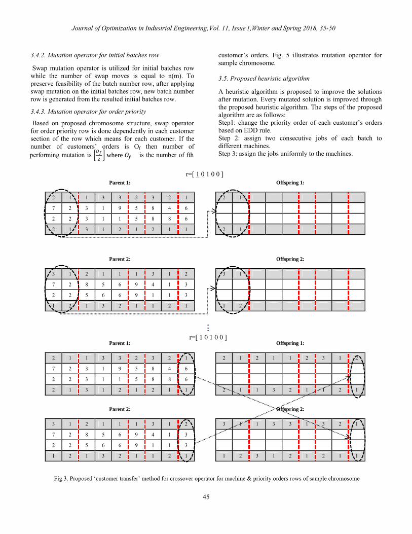
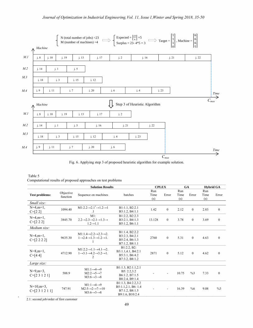
Applying first step may improve the tardiness costs. Second step may decrease the processing time because the resulted earlier start time cause to shorter processing time (processing time is linear function of start time) and may decrease tardiness costs. Third step may decrease machine deteriorating costs and tardiness costs because it avoids overload on one machine that lead to increased machine deteriorating costs and tardiness costs. It is obvious that presence of many jobs on one machine will increase the delay time of jobs to enter processing and so tardiness costs. Pseudo-code of Proposed Heuristic Algorithm is presented in Table 3. In order to assign the jobs uniformly to machines, i.e. applying step 3 we define expected and surplus measures. Expected is quotient of total number of jobs divided by number of machines and surplus=N-

m*Expected, i.e. expected determines the possible uniform assignment of jobs to machines and surplus calculates the number of additional jobs according to amount of expectede.g., if total number of jobs is 23 and number of machines is

Moreover, target measure is defined as a binary vector with length of number of machines×1 in which 0 means that expected number of jobs have assigned to corresponding machine and 1 means that one job besides the expected number of jobs has assigned to it. Finally, machine vector represents the assignment of jobs to machines. Fig 6. illustrates above-mentioned calculations for an example solution after applying step 3 of Heuristic Algorithm.

Fig 4. Proposed crossover operator for sample chromosomes

Parent 1:

2 1 1 3 3 2 3 2 1

7 2 3 1 9 5 8 4 6

2 2 3 1 1 5 8 8 6

2 1 3 1 2 1 2 1 1

Offspring 1:

2 1 2 1 1 2 3 1 2

2 1 1 3 2 1 1 2 1

Parent 1:

7 2 3 1 9 5 8 4 6

2 2 3 1 1 5 8 8 6

Offspring 1:

7 2 3 1 9 5 8 6 4

2 2 3 1 1 5 6 6 4

Parent 2:

3 1 2 1 1 1 3 1 2

7 2 8 5 6 9 4 1 3

2 2 5 6 6 9 1 1 3

1 2 1 3 2 1 1 2 1

Offspring 2:

3 1 1 3 3 1 3 2 1

1 2 3 1 2 1 2 1 1

Parent 2:

7 2 8 5 6 9 4 1 3

2 2 5 6 6 9 1 1 3

Offspring 2:

7 2 8 5 6 9 4 3 1

7 2 5 5 6 9 4 3 1

First stage crossover

Cross points={2,7}

Second stage crossover

4 then expected= ⌊23

4⌋ = 5 and surplus=23-4*5=3.

47

3.6. Details of the hybrid genetic algorithm 3.6.1. Input parameters Input parameters for the proposed Hybrid Genetic

Algorithm (HGA) are as follows:

Population size=80(HGA), 100(GA)

Max generation=100(HGA), 200(GA)

Probability of crossover=0.50

Probability of mutation=0.25

Probability of random solutions in each generation=0.05

Probability of elitist solutions selection=0.20

Pseudo-code of proposed Hybrid Genetic Algorithm is

presented in Table 4.

Fig 5. Proposed mutation operator for sample chromosome

4. Computational Results

In this section, we evaluate the performance of the suggested hybrid GA and traditional GA in comparison with the proposed MILP model. The proposed approaches are implemented in three cases (i.e., small, medium and large size test problems). It should be noted that according to the batch delivery scheduling problem literature, even in single machine case, excluding the deteriorating jobs and machines, CPLEX is only capable of solving small size problems (e.g., (Ahmadizar & Farhadi, 2015)). Consequently, the size of the test problems are defined regarding the high complexity of the problem. The proposed mathematical model is coded in the GAMS 24 optimization software which uses the CPLEX solver and all the empirical experiments are run on a Intel® core™ i5 2.67GHz processor with 4 GB memory RAM. Also, the time limitation of 7200 seconds are considered for each run of CPLEX. The implementation results are given in Table 5. From the results of Table 5 we can observe that in small size test problem CPLEX have a good performance, but, although CPLEX is one the most powerful commercial solvers for solving optimization models, because of the high complexity of the MILP model regarding the number of constraints, it is inefficient in when the size of the problem increases. Also, to evaluate the results, runtime of each method, as well as its error are reported. In order to calculate the amount of error for proposed metaheuristics, each algorithm is executed 25 times with different random initializations and results are recorded. Amount of error for GA and HGA algorithm is calculated by Eq. (20) in which soli is the solution of algorithm in the ith implementation and optimum is the best solution of algorithm among 30 different outcomes.

As can be seen from Table 5, in small and medium size problems, two metaheurisitics have similar performances but in the case of large size problem hybrid GA reaches the global solution in the less time and error in comparison with traditional genetic algorithm. As seen in this table, presence of multiple machines improves the amount of total costs in comparison with single machine, moreover hybrid genetic algorithm outperforms traditional genetic algorithm.

Parent :

2 1 1 3 3 2 3 2 1

7 2 3 1 9 5 8 4 6

2 2 3 1 1 5 8 8 6

2 1 3 1 2 1 2 1 1

2 1 1 3 3 2 3 2 1

7 2 3 1 9 5 8 4 6

2 1 3 1 2 1 2 1 1

Offspring :

2 1 3 3 3 2 1 1 1

7 1 3 2 9 8 5 4 6

7 7 3 2 9 8 4 4 6

1 2 2 1 3 1 1 2 1

Job transfer

Mutation operator

Swap

푒푟푟표푟 =1

25푠표푙 − 표푝푡푖푚푢푚

표푝푡푖푚푢푚 (20)



48

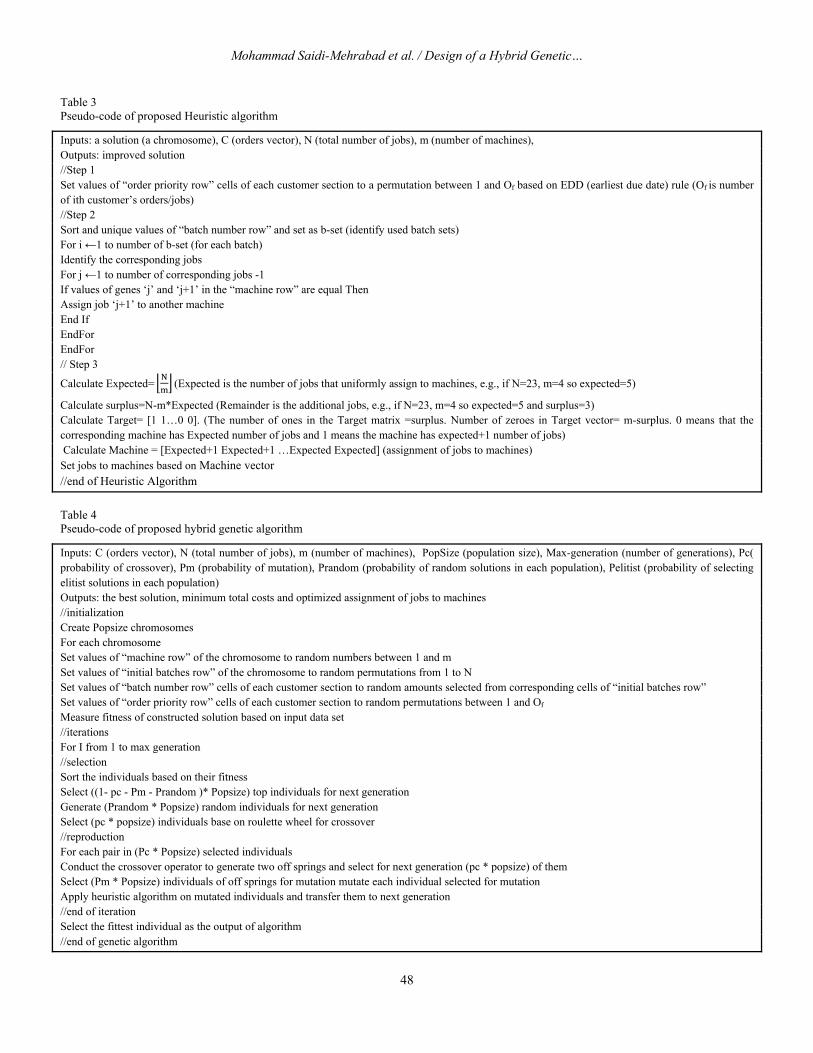
Table 3 Pseudo-code of proposed Heuristic algorithm

Inputs: a solution (a chromosome), C (orders vector), N (total number of jobs), m (number of machines), Outputs: improved solution //Step 1 Set values of “order priority row” cells of each customer section to a permutation between 1 and Of based on EDD (earliest due date) rule (Of is number of ith customer’s orders/jobs) //Step 2 Sort and unique values of “batch number row” and set as b-set (identify used batch sets) For i ←1 to number of b-set (for each batch) Identify the corresponding jobs For j ←1 to number of corresponding jobs -1 If values of genes ‘j’ and ‘j+1’ in the “machine row” are equal Then Assign job ‘j+1’ to another machine End If EndFor EndFor // Step 3

Calculate Expected= (Expected is the number of jobs that uniformly assign to machines, e.g., if N=23, m=4 so expected=5)

Calculate surplus=N-m*Expected (Remainder is the additional jobs, e.g., if N=23, m=4 so expected=5 and surplus=3) Calculate Target= [1 1…0 0]. (The number of ones in the Target matrix =surplus. Number of zeroes in Target vector= m-surplus. 0 means that the corresponding machine has Expected number of jobs and 1 means the machine has expected+1 number of jobs) Calculate Machine = [Expected+1 Expected+1 …Expected Expected] (assignment of jobs to machines) Set jobs to machines based on Machine vector //end of Heuristic Algorithm

Table 4 Pseudo-code of proposed hybrid genetic algorithm

Inputs: C (orders vector), N (total number of jobs), m (number of machines), PopSize (population size), Max-generation (number of generations), Pc( probability of crossover), Pm (probability of mutation), Prandom (probability of random solutions in each population), Pelitist (probability of selecting elitist solutions in each

population)

Outputs: the best solution, minimum total costs and optimized assignment of jobs to machines //initialization Create Popsize chromosomes For each chromosome Set values of “machine row” of the chromosome to random numbers between 1 and m Set values of “initial batches row” of the chromosome to random permutations from 1 to N Set values of “batch number row” cells of each customer section to random amounts selected from corresponding cells of “initial batches row” Set values of “order priority row” cells of each customer section to random permutations between 1 and Of

Measure fitness of constructed solution based on input data set //iterations For I from 1 to max generation //selection Sort the individuals based on their fitness Select ((1- pc - Pm - Prandom )* Popsize) top individuals for next generation Generate (Prandom * Popsize) random individuals for next generation Select (pc * popsize) individuals base on roulette wheel for crossover //reproduction For each pair in (Pc * Popsize) selected individuals Conduct the crossover operator to generate two off springs and select for next generation (pc * popsize) of them Select (Pm * Popsize) individuals of off springs for mutation mutate each individual selected for mutation Apply heuristic algorithm on mutated individuals and transfer them to next generation //end of iteration Select the fittest individual as the output of algorithm //end of genetic algorithm

⌊N

m⌋

49

Fig. 6. Applying step 3 of proposed heuristic algorithm for example solution.

Table 5 Computational results of proposed approaches on test problems

Solution Results CPLEX GA Hybrid GA

Test problems: Objective function

Sequence on machines batches Run Time

(s) Error

Run Time

(s) Error

Run Time

(s) Error

Small size: N=4,m=1, C=[2 2]

1094.40 M1:2.2→2.1*→1.2→1

.1 B1:1.1, B2:2.1 B3:1.2, B4:1.1

1.42 0 2.12 0 2.83 0

N=4,m=1, C=[2 2 2]

3845.70 M1:

2.2→2.3→2.1→1.3→1.2→1.1

B1:2.2, B2:2.3 B3:2.1, B4:1.3 B5:1.2, B6:1.1

13.128 0 3.78 0 3.69 0

Medium size:

N=4,m=1, C=[2 2 2 2]

9635.30 M1:1.4→2.2→2.3→2.1→2.4→1.3→1.2→1.

1

B1:1.4, B2:2.2 B3:2.3, B4:2.1 B5:2.4, B6:1.3 B7:1.2, B8:1.1

2760 0 5.31 0 4.63 0

N=8,m=1, C=[4 4]

4712.90 M1:2.2→1.1→4.1→2.1→3.1→4.2→3.2→1.

2

B1:2.2, B2: B3:1.1,4.1, B4:2.1

B5:3.1, B6:4.2 B7:3.2, B8:1.2

2871 0 5.12 0 4.62 0

Large size:

N=9,m=3, C=[2 3 1 2 1]

588.9 M1:1→4→9 M2:2→5→7 M3:6→3→8

B1:1.3, B2:1.1,2.1 B5: 2.2,3.2

B6:1.2, B7:1.5 B8:2.4, B9:1.4

- - 10.75 %3 7.33 0

N=10,m=3, C=[2 3 1 2 1 1]

747.91 M1:1→4→9

M2:5→2→7→10 M3:6→3→8

B1:1.3, B4:2.2,3.2 B5:1.1,2.1, B6: 1.4

B7:1.2, B8:1.5 B9:1.6, B10:2.4

- - 16.39 %6 9.08 %3

* 2.1: second job/order of first customer

Step 3 of Heuristic Algorithm

Cmax

Machine

Time

j. 14 j. 1

j. 19 M.1

j. 18

j. 9

j. 3 j. 15

j. 11 j. 7

M.2

M.3

j. 8 j. 10

M.4

j. 13 j. 17 j. 2

j. 16 j. 21 j. 22j. 5

j. 12

j. 20 j. 6

j. 23j. 4

Cmax

Machine

Time

j. 14 j. 1

j. 19 M.1

j. 18

j. 9

j. 3 j. 15

j. 11 j. 7

M.2

M.3

j. 8 j. 10

M.4

j. 13 j. 17 j. 2 j. 16 j. 21 j. 22

j. 5

j. 12

j. 20 j. 6 j. 23j. 4

N (total number of jobs) =23

M (number of machines) =4

Expected = ⌊23

4⌋ =5

Surplus = 23- 4*5 = 3Target =

1110

, Machine =

6665



50

References

Ahmadizar, F. & Farhadi, S. (2015). Single-machine batch delivery scheduling with job release dates, due windows and earliness, tardiness, holding and delivery costs. Computers & Operations Research, 53, 194-205.

Bandyopadhyay, S. & Bhattacharya, R. (2013). Solving multi-objective parallel machine scheduling problem by a modified NSGA-II. Applied Mathematical Modelling, 37 (10), 6718-6729.

Cheng, T. & Kahlbacher, H. (1993). Scheduling with delivery and earliness penalties. Asia-Pacific Journal of Operational Research, 10 (2), 145-152.

Davis, L. & Coombs, S. (1987). Genetic algorithms and communication link speed design: theoretical considerations. Paper presented at the Genetic algorithms and their applications: proceedings of the second International Conference on Genetic Algorithms: July 28-31, 1987 at the Massachusetts Institute of Technology, Cambridge, MA.

Graham, F., Smiley, J., Russell, W. & Nairn, R. (1977). Characteristics of a human cell line transformed by DNA from human adenovirus type 5. Journal of General Virology, 36(1), 59-72.

Hall, N. G., & Potts, C. N. (2003). Supply chain scheduling: Batching and delivery. Operations Research, 51(4), 566-584.

Hamidinia, A. Khakabimamaghani, S., Mazdeh, M. M., & Jafari, M. (2012). A genetic algorithm for minimizing total tardiness/earliness of weighted jobs in a batched delivery system. Computers & Industrial Engineering, 62 (1), 29-38.

Karimi, N. & Davoudpour, H. (2015). A branch and bound method for solving multi-factory supply chain scheduling with batch delivery. Expert Systems with Applications, 42 (1), 238-245.

Mazdeh, M. M., Rostami, M., & Namaki, M. H. (2013). Minimizing maximum tardiness and delivery costs in a batched delivery system. Computers & Industrial Engineering, 66(4), 675-682.

Mazdeh, M. M., Sarhadi, M., & Hindi, K. S. (2007). A branch-and-bound algorithm for single-machine scheduling with batch delivery minimizing flow times and delivery costs. European Journal of Operational Research, 183(1), 74-86.

Mazdeh, M. M., Shashaani, S., Ashouri, A., & Hindi, K. S. (2011). Single-machine batch scheduling minimizing weighted flow times and delivery costs. Applied Mathematical Modelling, 35(1), 563-570.

Mazdeh, M. M., Zaerpour, F., Zareei, A., & Hajinezhad, A. (2010). Parallel machines scheduling to minimize job tardiness and machine deteriorating cost with deteriorating jobs. Applied Mathematical Modelling, 34(6), 1498-1510.

Talbi, E.-G. (2009). Metaheuristics: from design to implementation (Vol. 74): John Wiley & Sons.

Wang, G., & Cheng, T. E. (2000). Parallel machine scheduling with batch delivery costs. International Journal of Production Economics, 68(2), 177-183.

Yin, Y., Ye, D. & Zhang, G. (2014). Single machine batch scheduling to minimize the sum of total flow time and batch delivery cost with an unavailability interval. Information Sciences, 274, 310-322.

This article can be cited: Saidi-Mehrabad, M. &, Bairamzadeh S. (2018). Design of a Hybrid Genetic Algorithm for Parallel Machines Scheduling to Minimize Job Tardiness and Machine Deteriorating Costs with Deteriorating Jobs in a Bbatched Ddelivery System .Journal of Optimization in Industrial Engineering.11 (1), 35- 50.

URL: http://www.qjie.ir/article_272.html DOI:10.22094/JOIE.2018.272

Documents

Design of a Hybrid Genetic Algorithm for Parallel Machines ... · genetic algorithm for single-machine batch delivery scheduling problem with the objectives of minimizing the