Embed Size (px)
Citation preview
Genetic Algorithms
And other approaches for similar applications
Optimization Techniques

Optimization TechniquesOptimization Techniques• Mathematical ProgrammingMathematical Programming• Network AnalysisNetwork Analysis• Branch & Bound Branch & Bound • Genetic AlgorithmGenetic Algorithm• Simulated AnnealingSimulated Annealing• Tabu SearchTabu Search
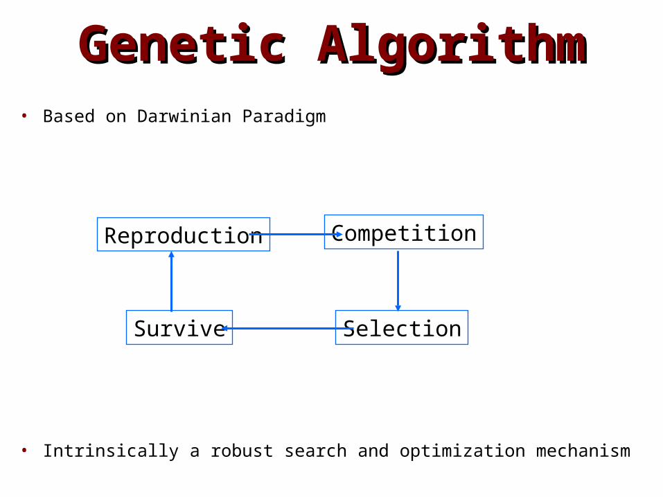
Genetic AlgorithmGenetic Algorithm• Based on Darwinian Paradigm
• Intrinsically a robust search and optimization mechanism
Reproduction Competition
SelectionSurvive
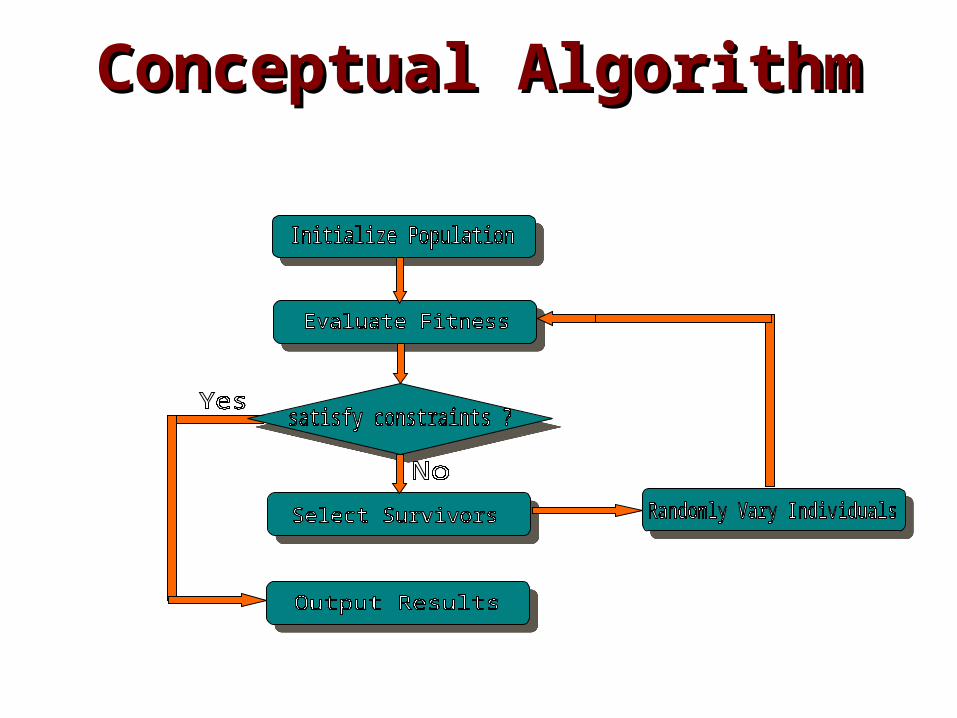
Conceptual AlgorithmConceptual Algorithm
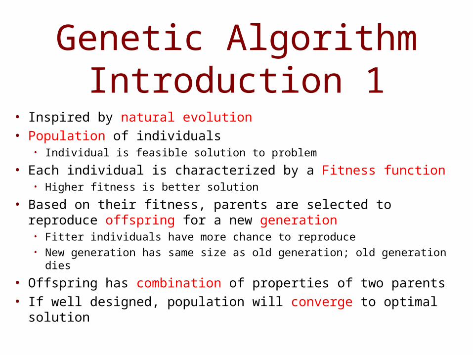
Genetic Algorithm Introduction 1
• Inspired by natural evolution• Population of individuals
• Individual is feasible solution to problem• Each individual is characterized by a Fitness function
• Higher fitness is better solution• Based on their fitness, parents are selected to reproduce
offspring for a new generation• Fitter individuals have more chance to reproduce• New generation has same size as old generation; old generation dies
• Offspring has combination of properties of two parents• If well designed, population will converge to optimal
solution
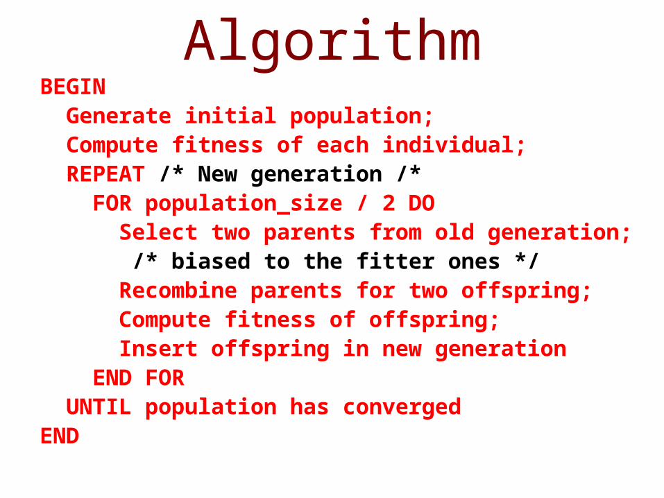
AlgorithmBEGIN Generate initial population; Compute fitness of each individual; REPEAT /* New generation /* FOR population_size / 2 DO Select two parents from old generation; /* biased to the fitter ones */ Recombine parents for two offspring; Compute fitness of offspring; Insert offspring in new generation END FOR UNTIL population has convergedEND
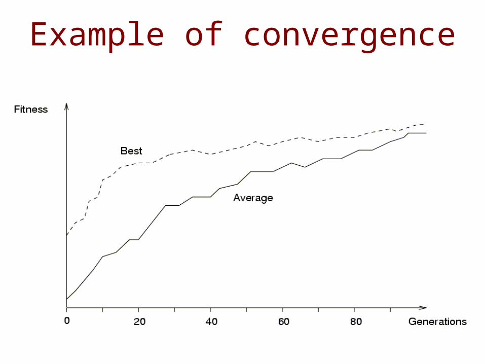
Example of convergence
Introduction 2• Reproduction mechanisms have no
knowledge of the problem to be solved
• Link between genetic algorithm and problem:• Coding• Fitness function
Basic principles 1• Coding or Representation
• String with all parameters• Fitness function
• Parent selection• Reproduction
• Crossover• Mutation
• Convergence• When to stop
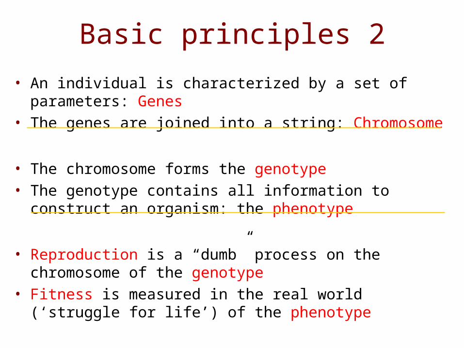
Basic principles 2• An individual is characterized by a set of parameters:
Genes• The genes are joined into a string: Chromosome
• The chromosome forms the genotype• The genotype contains all information to construct
an organism: the phenotype
• Reproduction is a “dumb” process on the chromosome of the genotype
• Fitness is measured in the real world (‘struggle for life’) of the phenotype
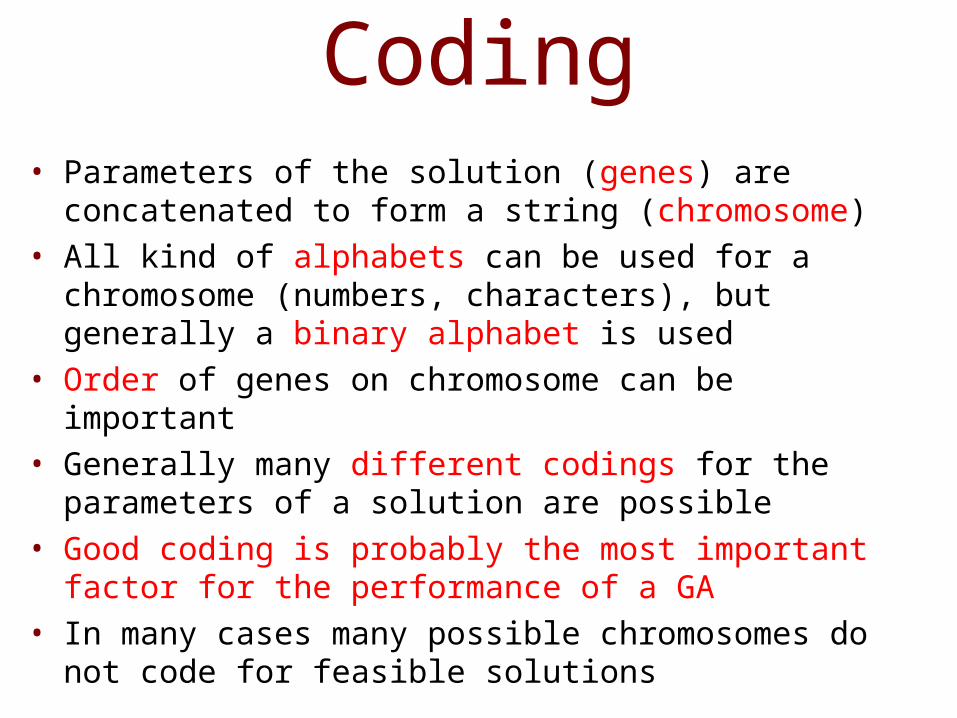
Coding• Parameters of the solution (genes) are concatenated
to form a string (chromosome)• All kind of alphabets can be used for a chromosome
(numbers, characters), but generally a binary alphabet is used
• Order of genes on chromosome can be important• Generally many different codings for the parameters
of a solution are possible• Good coding is probably the most important factor
for the performance of a GA• In many cases many possible chromosomes do not
code for feasible solutions
Genetic AlgorithmGenetic Algorithm• Encoding• Fitness Evaluation• Reproduction• Survivor Selection
Encoding Encoding • Design alternative individual
(chromosome)• Single design choice gene• Design objectives fitness
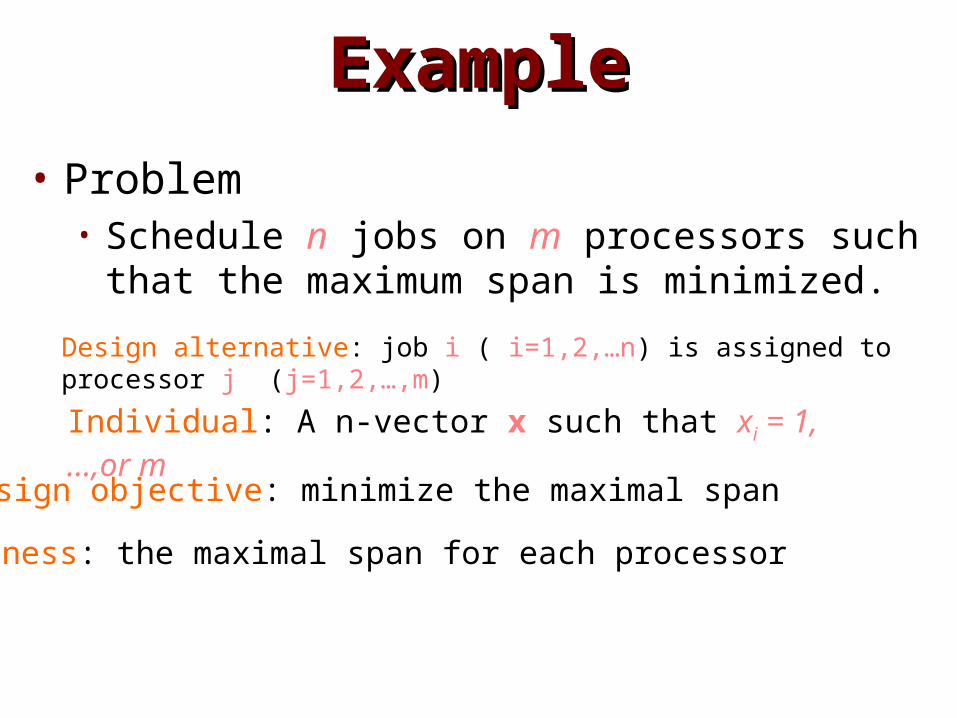
ExampleExample• Problem
• Schedule n jobs on m processors such that the maximum span is minimized.
Design alternative: job i ( i=1,2,…n) is assigned to processor j (j=1,2,…,m)
Individual: A n-vector x such that xi = 1, …,or m
Design objective: minimize the maximal span
Fitness: the maximal span for each processor
Reproduction•Reproduction operators
• Crossover• Mutation
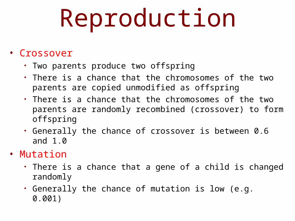
Reproduction• Crossover
• Two parents produce two offspring• There is a chance that the chromosomes of the two parents
are copied unmodified as offspring• There is a chance that the chromosomes of the two parents
are randomly recombined (crossover) to form offspring• Generally the chance of crossover is between 0.6 and 1.0
• Mutation• There is a chance that a gene of a child is changed randomly• Generally the chance of mutation is low (e.g. 0.001)
Reproduction Operators• Crossover
• Generating offspring from two selected parentsSingle point crossoverTwo point crossover (Multi point crossover)Uniform crossover
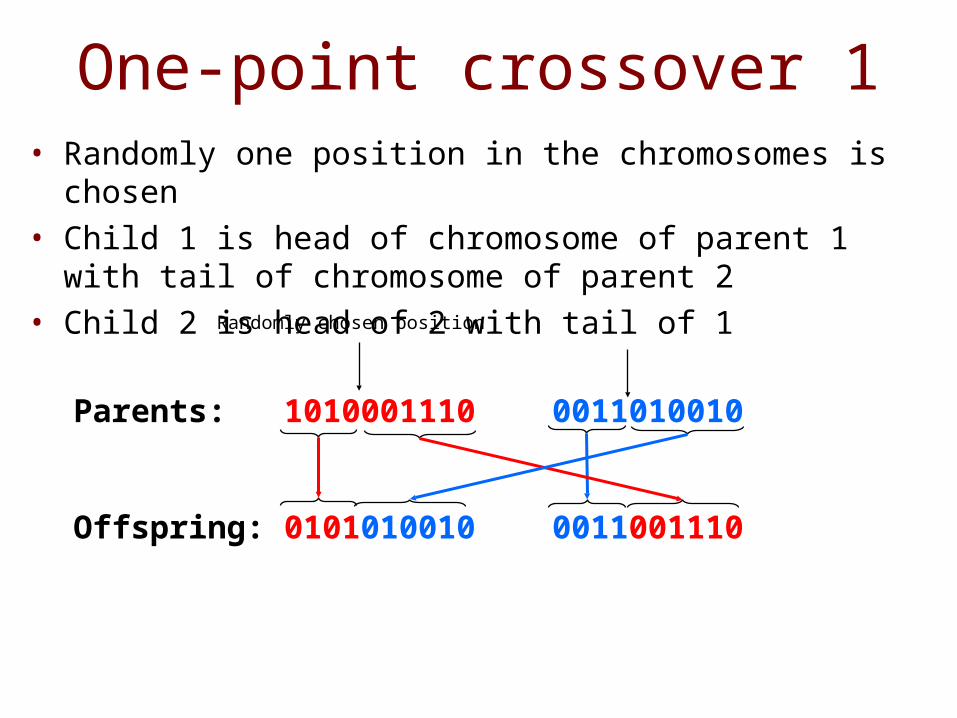
One-point crossover 1• Randomly one position in the chromosomes is
chosen• Child 1 is head of chromosome of parent 1 with tail
of chromosome of parent 2• Child 2 is head of 2 with tail of 1
Parents: 1010001110 0011010010
Offspring: 0101010010 0011001110
Randomly chosen position
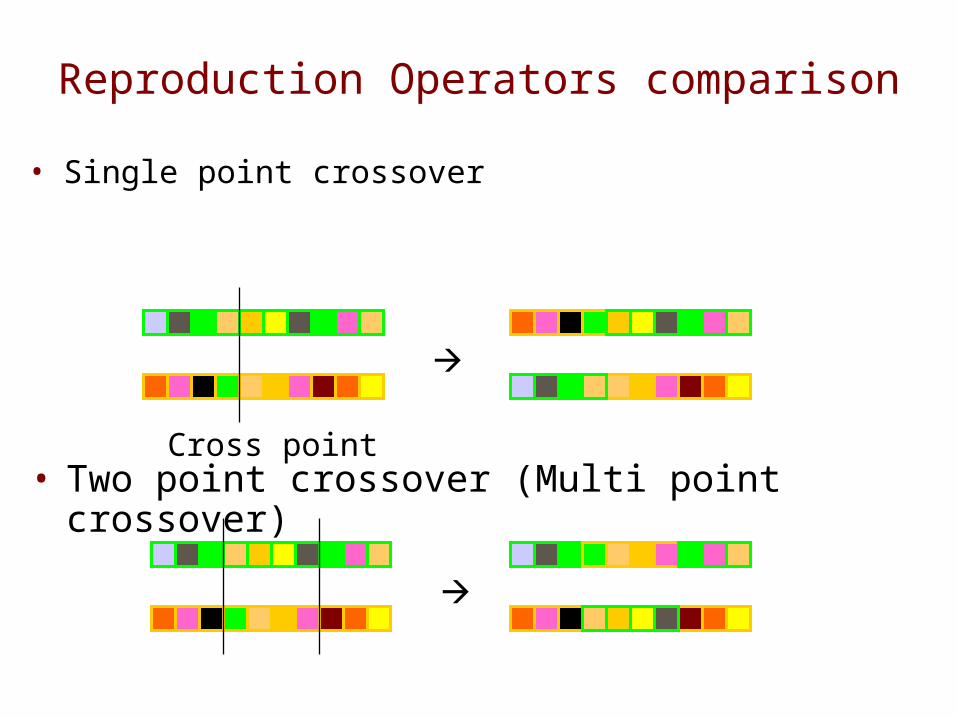
Reproduction Operators comparison• Single point crossover
Cross point
• Two point crossover (Multi point crossover)
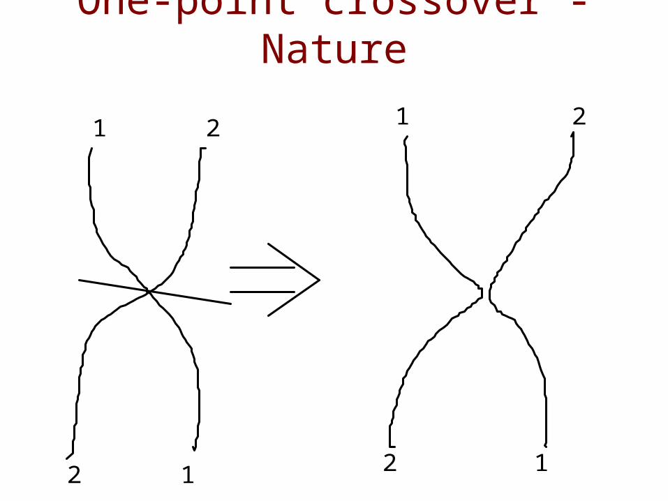
One-point crossover - Nature1 2
12
1
2
2
1
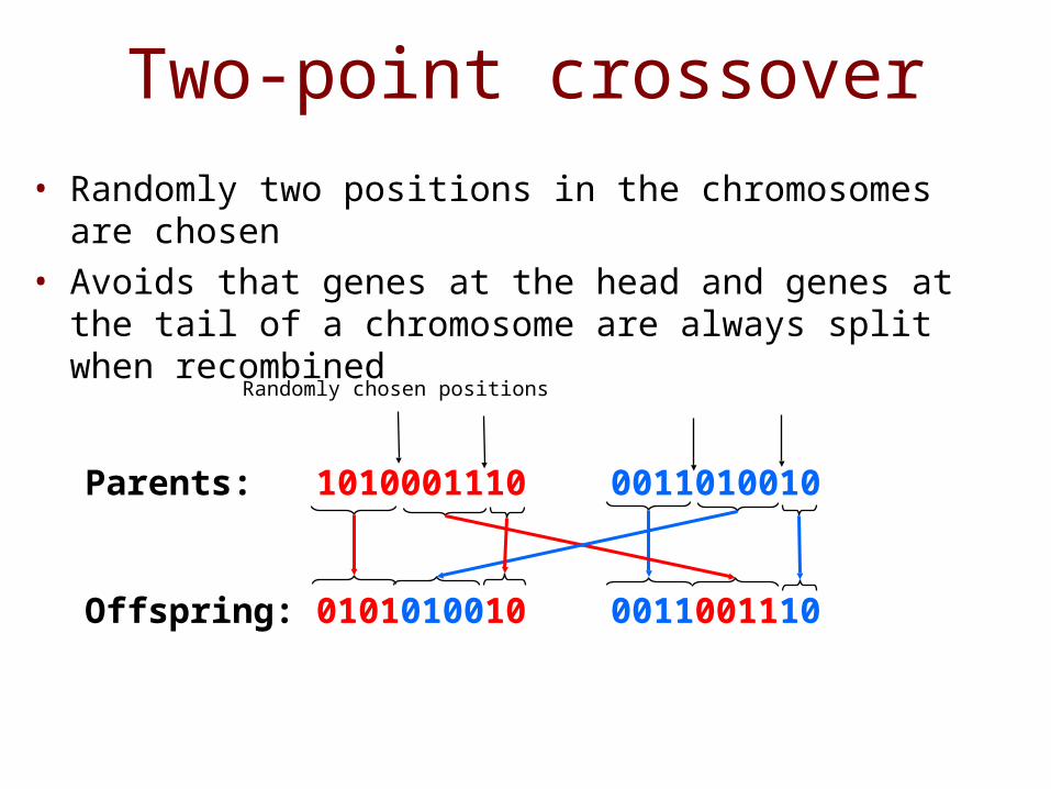
Two-point crossover
Parents: 1010001110 0011010010
Offspring: 0101010010 0011001110
Randomly chosen positions
• Randomly two positions in the chromosomes are chosen
• Avoids that genes at the head and genes at the tail of a chromosome are always split when recombined
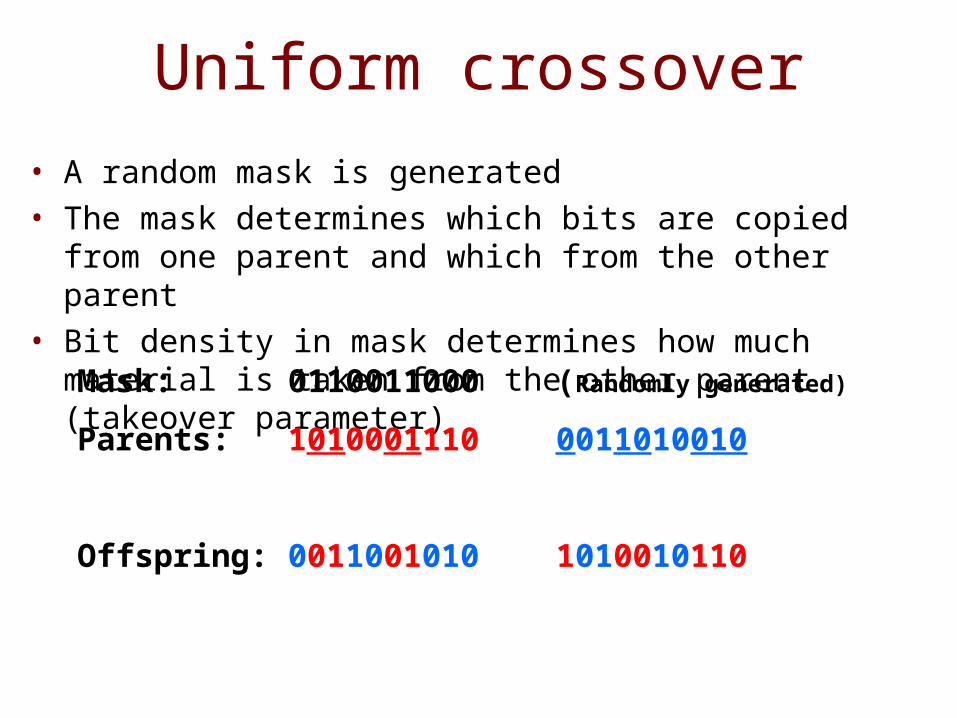
Uniform crossover• A random mask is generated• The mask determines which bits are copied from one
parent and which from the other parent• Bit density in mask determines how much material is
taken from the other parent (takeover parameter)Mask: 0110011000 (Randomly generated)
Parents: 1010001110 0011010010
Offspring: 0011001010 1010010110
Reproduction Operators
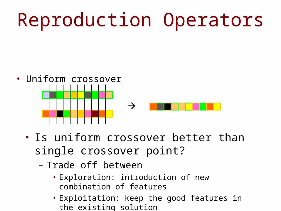
• Uniform crossover
• Is uniform crossover better than single crossover point?– Trade off between
• Exploration: introduction of new combination of features• Exploitation: keep the good features in the existing solution
Problems with crossover• Depending on coding, simple crossovers can have
high chance to produce illegal offspring• E.g. in TSP with simple binary or path coding, most offspring
will be illegal because not all cities will be in the offspring and some cities will be there more than once
• Uniform crossover can often be modified to avoid this problem• E.g. in TSP with simple path coding:
Where mask is 1, copy cities from one parent Where mask is 0, choose the remaining cities in the order of the
other parent
Reproduction Operators
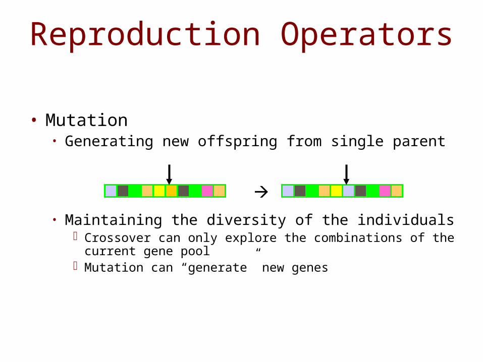
• Mutation• Generating new offspring from single parent
• Maintaining the diversity of the individualsCrossover can only explore the combinations of the
current gene poolMutation can “generate” new genes
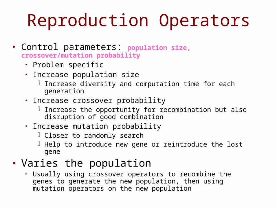
Reproduction Operators• Control parameters: population size,
crossover/mutation probability• Problem specific• Increase population size
Increase diversity and computation time for each generation
• Increase crossover probability Increase the opportunity for recombination but also
disruption of good combination• Increase mutation probability
Closer to randomly search Help to introduce new gene or reintroduce the lost gene
• Varies the population• Usually using crossover operators to recombine the genes to
generate the new population, then using mutation operators on the new population
Parent/Survivor Selection
• Strategies• Survivor selection
Always keep the best oneElitist: deletion of the K worstProbability selection : inverse to their
fitnessEtc.
Parent/Survivor Selection
• Too strong fitness selection bias can lead to sub-optimal solution
• Too little fitness bias selection results in unfocused and meandering search
Parent selectionChance to be selected as parent proportional to
fitness• Roulette wheel
To avoid problems with fitness function• Tournament
Not a very important parameter
Parent/Survivor Selection
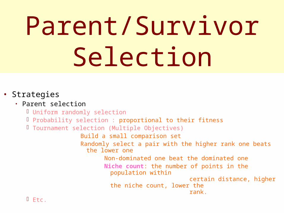
• Strategies• Parent selection
Uniform randomly selection Probability selection : proportional to their fitness Tournament selection (Multiple Objectives)
Build a small comparison setRandomly select a pair with the higher rank one beats the lower
oneNon-dominated one beat the dominated oneNiche count: the number of points in the population
within certain distance, higher the niche count, lower the rank.
Etc.
Others
• Global Optimal• Parameter Tuning• Parallelism• Random number generators
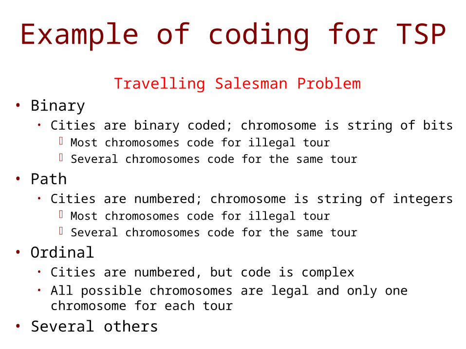
Example of coding for TSPTravelling Salesman Problem
• Binary• Cities are binary coded; chromosome is string of bits
Most chromosomes code for illegal tour Several chromosomes code for the same tour
• Path• Cities are numbered; chromosome is string of integers
Most chromosomes code for illegal tour Several chromosomes code for the same tour
• Ordinal• Cities are numbered, but code is complex• All possible chromosomes are legal and only one chromosome
for each tour• Several others
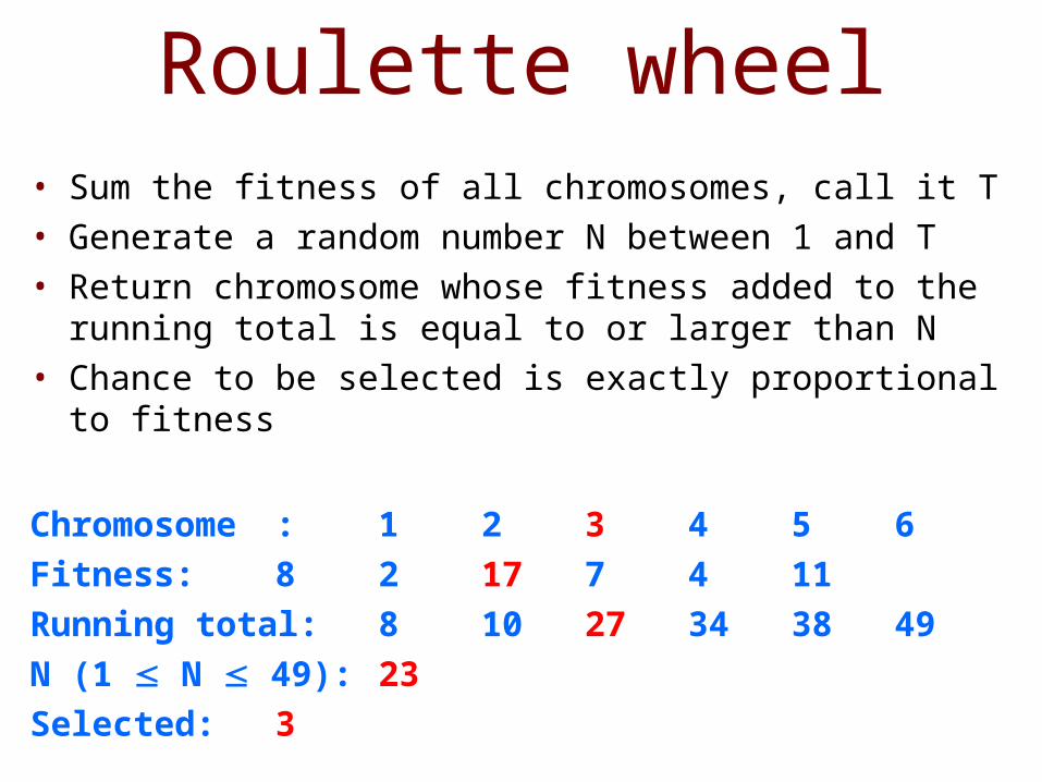
Roulette wheel• Sum the fitness of all chromosomes, call it T• Generate a random number N between 1 and T• Return chromosome whose fitness added to the
running total is equal to or larger than N• Chance to be selected is exactly proportional to
fitness
Chromosome : 1 2 3 4 5 6Fitness: 8 2 17 7 4 11Running total: 8 10 27 34 38 49N (1 N 49): 23Selected: 3
Tournament• Binary tournament
• Two individuals are randomly chosen; the fitter of the two is selected as a parent
• Probabilistic binary tournament• Two individuals are randomly chosen; with a chance p,
0.5<p<1, the fitter of the two is selected as a parent• Larger tournaments
• n individuals are randomly chosen; the fittest one is selected as a parent
• By changing n and/or p, the GA can be adjusted dynamically
Problems with fitness range• Premature convergence
Fitness too large• Relatively superfit individuals dominate population• Population converges to a local maximum• Too much exploitation; too few exploration
• Slow finishing Fitness too small• No selection pressure• After many generations, average fitness has converged, but
no global maximum is found; not sufficient difference between best and average fitness
• Too few exploitation; too much exploration
Solutions for these problems • Use tournament selection
• Implicit fitness remapping• Adjust fitness function for roulette
wheel• Explicit fitness remapping
Fitness scalingFitness windowingFitness ranking
Will be explained below
Fitness FunctionPurpose• Parent selection• Measure for convergence• For Steady state: Selection of individuals to die
• Should reflect the value of the chromosome in some “real” way
• Next to coding the most critical part of a GA
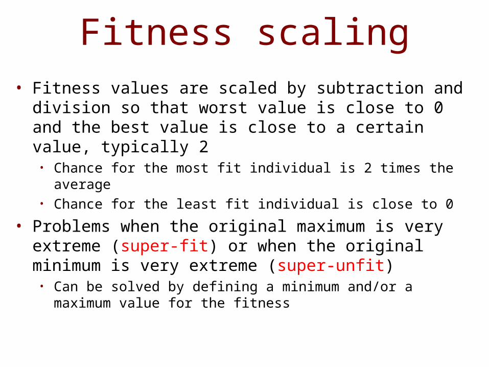
Fitness scaling• Fitness values are scaled by subtraction and division
so that worst value is close to 0 and the best value is close to a certain value, typically 2• Chance for the most fit individual is 2 times the average• Chance for the least fit individual is close to 0
• Problems when the original maximum is very extreme (super-fit) or when the original minimum is very extreme (super-unfit)• Can be solved by defining a minimum and/or a maximum
value for the fitness
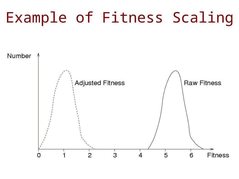
Example of Fitness Scaling
Fitness windowing• Same as window scaling, except
the amount subtracted is the minimum observed in the n previous generations, with n e.g. 10
• Same problems as with scaling
Fitness ranking
• Individuals are numbered in order of increasing fitness
• The rank in this order is the adjusted fitness• Starting number and increment can be chosen
in several ways and influence the results
• No problems with super-fit or super-unfit• Often superior to scaling and windowing
Fitness EvaluationFitness Evaluation• A key component in GA• Time/quality trade off• Multi-criterion fitness
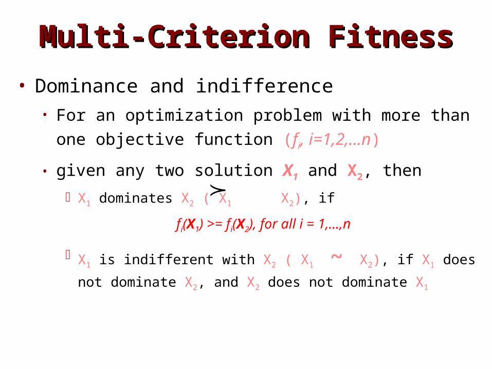
Multi-Criterion FitnessMulti-Criterion Fitness• Dominance and indifference
• For an optimization problem with more than one objective function (fi, i=1,2,…n)
• given any two solution X1 and X2, thenX1 dominates X2 ( X1 X2), if
fi(X1) >= fi(X2), for all i = 1,…,n
X1 is indifferent with X2 ( X1 ~ X2), if X1 does not dominate X2, and X2 does not dominate X1
Multi-Criterion FitnessMulti-Criterion Fitness• Pareto Optimal Set
• If there exists no solution in the search space which dominates any member in the set P, then the solutions belonging the the set P constitute a global Pareto-optimal set.
• Pareto optimal front• Dominance Check
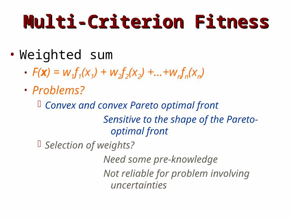
Multi-Criterion FitnessMulti-Criterion Fitness• Weighted sum
• F(x) = w1f1(x1) + w2f2(x2) +…+wnfn(xn)• Problems?
Convex and convex Pareto optimal frontSensitive to the shape of the
Pareto-optimal frontSelection of weights?
Need some pre-knowledge Not reliable for problem involving
uncertainties
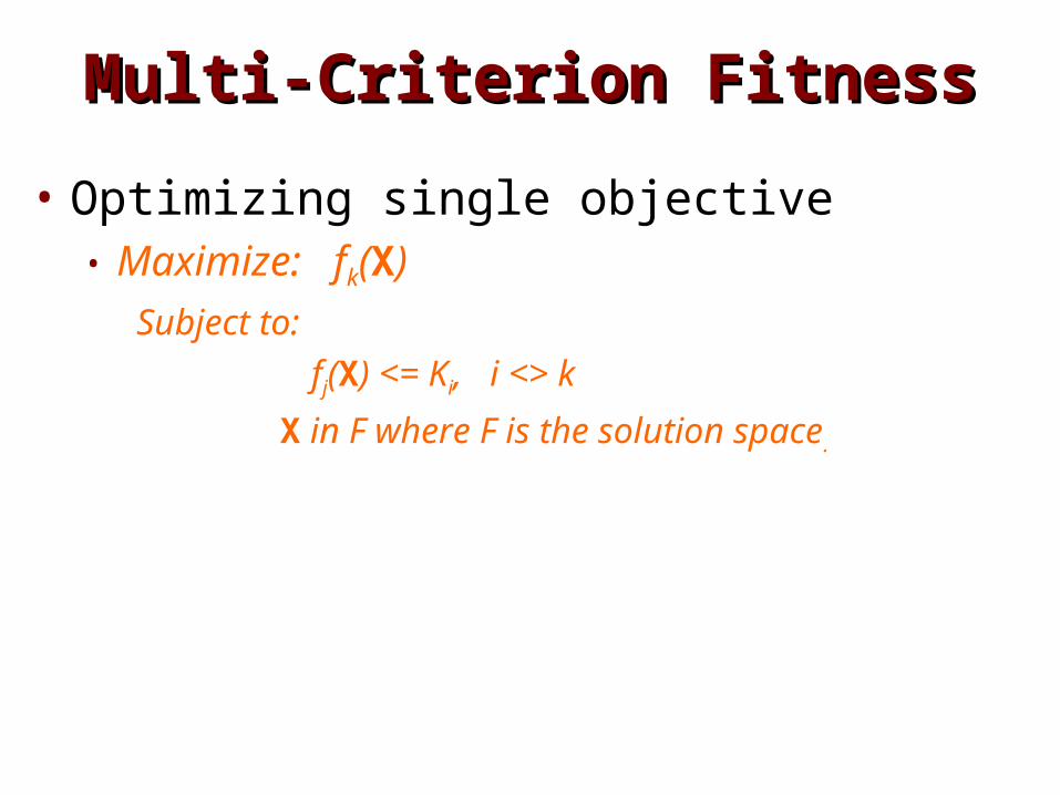
Multi-Criterion FitnessMulti-Criterion Fitness• Optimizing single objective
• Maximize: fk(X)Subject to: fj(X) <= Ki, i <> k
X in F where F is the solution space.
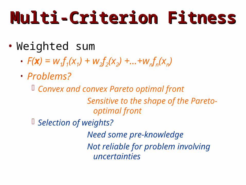
Multi-Criterion FitnessMulti-Criterion Fitness• Weighted sum
• F(x) = w1f1(x1) + w2f2(x2) +…+wnfn(xn)• Problems?
Convex and convex Pareto optimal frontSensitive to the shape of the
Pareto-optimal frontSelection of weights?
Need some pre-knowledge Not reliable for problem involving
uncertainties
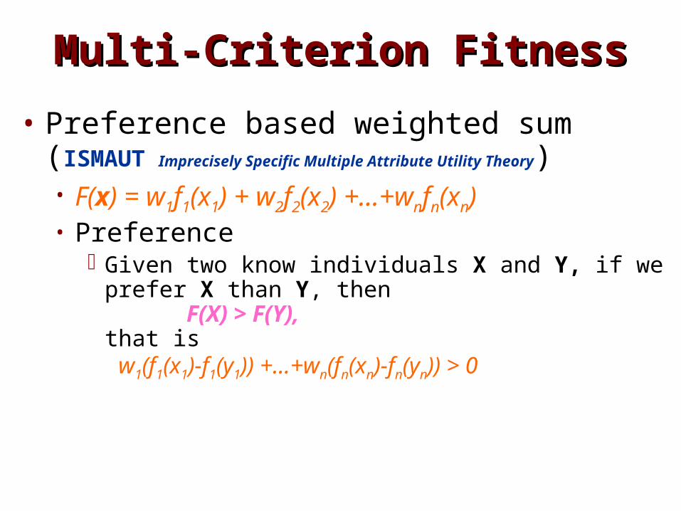
Multi-Criterion FitnessMulti-Criterion Fitness• Preference based weighted sum
(ISMAUT Imprecisely Specific Multiple Attribute Utility Theory) • F(x) = w1f1(x1) + w2f2(x2) +…+wnfn(xn)• Preference
Given two know individuals X and Y, if we prefer X than Y, then F(X) > F(Y), that is w1(f1(x1)-f1(y1)) +…+wn(fn(xn)-fn(yn)) > 0
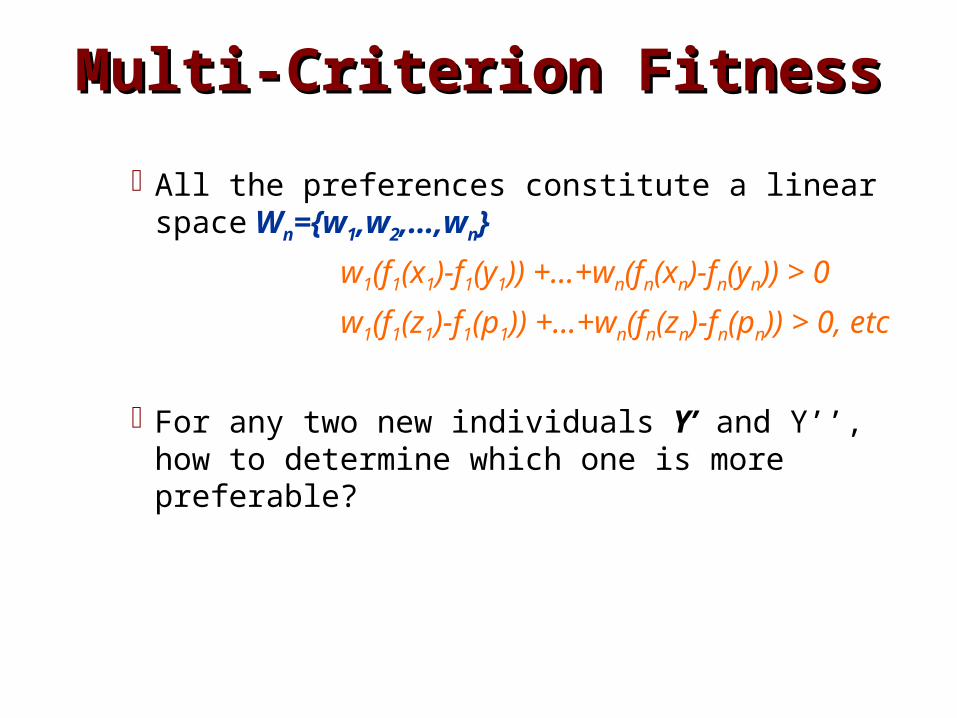
All the preferences constitute a linear space Wn={w1,w2,…,wn}
w1(f1(x1)-f1(y1)) +…+wn(fn(xn)-fn(yn)) > 0
w1(f1(z1)-f1(p1)) +…+wn(fn(zn)-fn(pn)) > 0, etc
For any two new individuals Y’ and Y’’, how to determine which one is more preferable?
Multi-Criterion FitnessMulti-Criterion Fitness
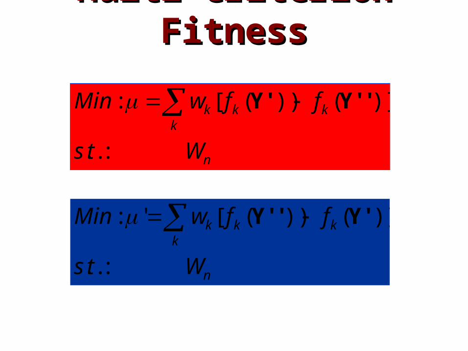
Multi-Criterion FitnessMulti-Criterion Fitness
n
kkkk
Wts
ffwMin
:..
)]())([: 'Y'Y'
n
kkkk
Wts
ffwMin
:..
)]())([': Y''Y'
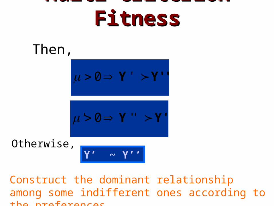
Multi-Criterion FitnessMulti-Criterion Fitness
'Y'Y '0
Y'Y ''0'
Then,
Otherwise, Y’ ~ Y’’
Construct the dominant relationship among some indifferent ones according to the preferences.
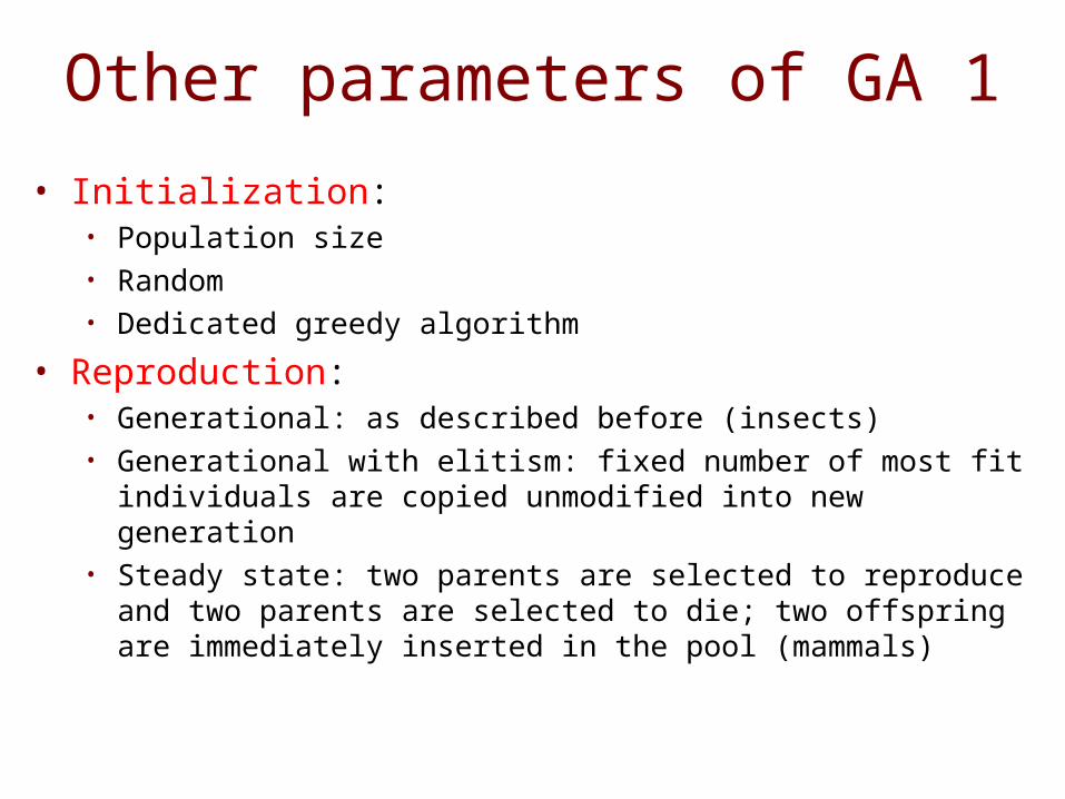
Other parameters of GA 1• Initialization:
• Population size• Random• Dedicated greedy algorithm
• Reproduction: • Generational: as described before (insects)• Generational with elitism: fixed number of most fit
individuals are copied unmodified into new generation• Steady state: two parents are selected to reproduce and two
parents are selected to die; two offspring are immediately inserted in the pool (mammals)
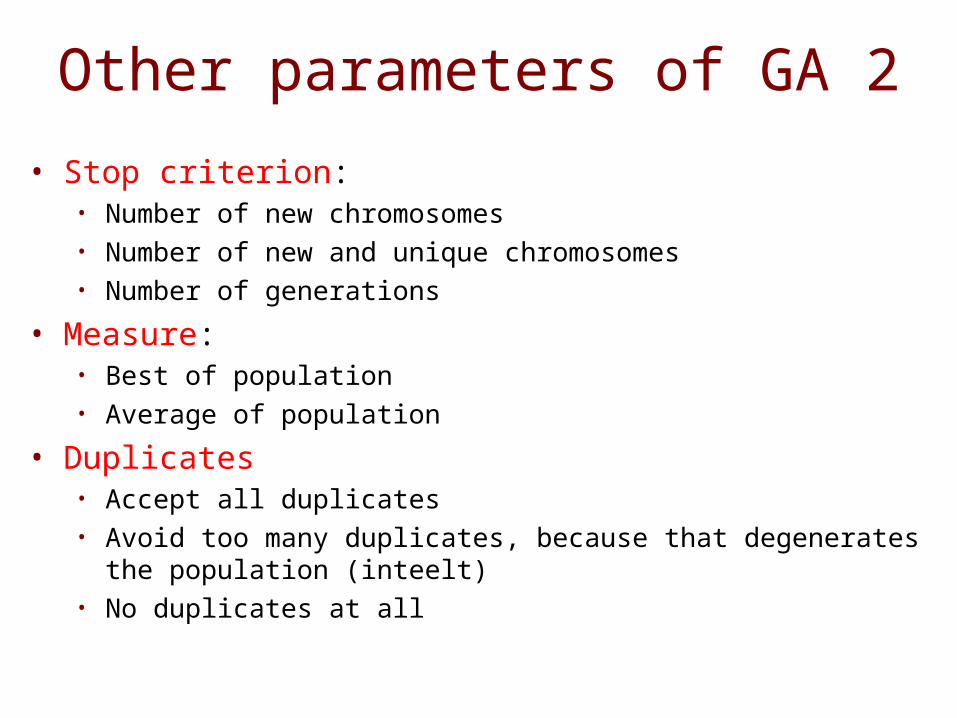
Other parameters of GA 2• Stop criterion:
• Number of new chromosomes• Number of new and unique chromosomes• Number of generations
• Measure:• Best of population• Average of population
• Duplicates• Accept all duplicates• Avoid too many duplicates, because that degenerates the
population (inteelt)• No duplicates at all
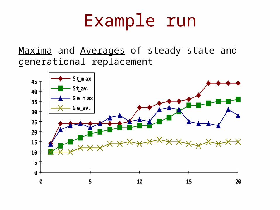
Example runMaxima and Averages of steady state and generational replacement
05
1015202530354045
0 5 10 15 20
St_maxSt_av.Ge_maxGe_av.

Simulated Annealing
• What• Exploits an analogy between the
annealing process and the search for the optimum in a more general system.

Annealing Process• Annealing Process
• Raising the temperature up to a very high level (melting temperature, for example), the atoms have a higher energy state and a high possibility to re-arrange the crystalline structure.
• Cooling down slowly, the atoms have a lower and lower energy state and a smaller and smaller possibility to re-arrange the crystalline structure.

Simulated Annealing• Analogy
• Metal Problem• Energy State Cost Function• Temperature Control Parameter• A completely ordered crystalline structure
the optimal solution for the problem
Global optimal solution can be achieved as long as the cooling process is slow enough.
Metropolis Loop• The essential characteristic of simulated
annealing• Determining how to randomly explore new
solution, reject or accept the new solutionat a constant temperature T.
• Finished until equilibrium is achieved.
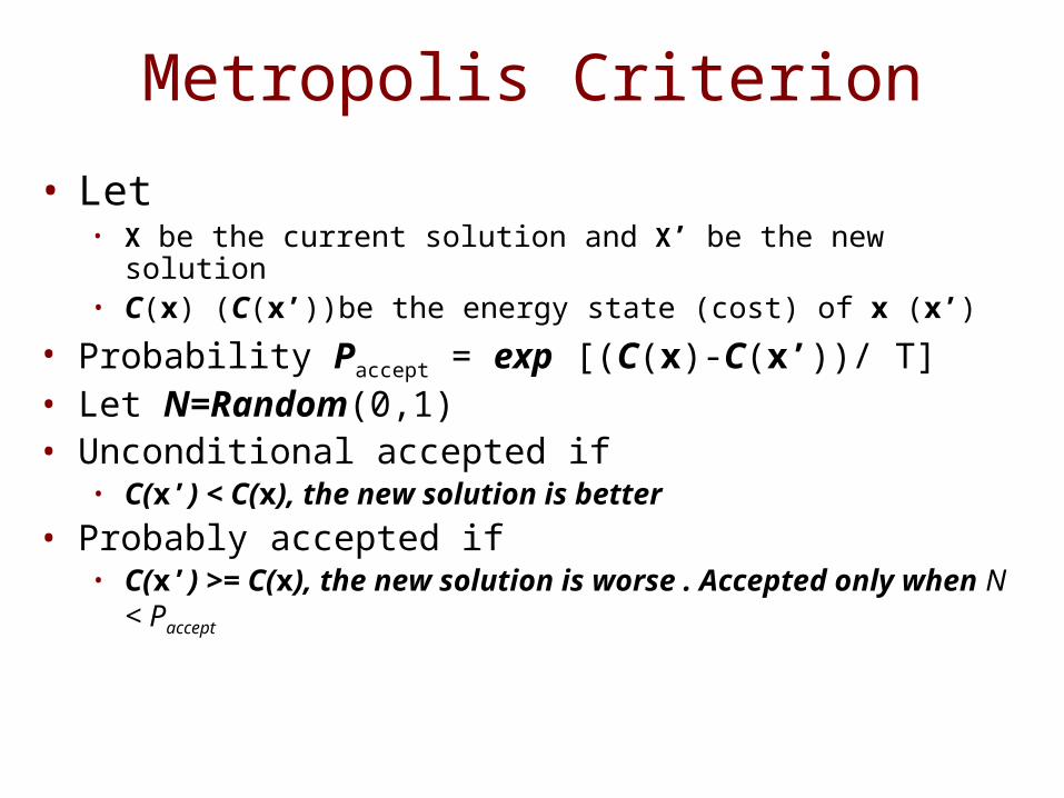
Metropolis Criterion• Let
• X be the current solution and X’ be the new solution• C(x) (C(x’))be the energy state (cost) of x (x’)
• Probability Paccept = exp [(C(x)-C(x’))/ T]• Let N=Random(0,1)• Unconditional accepted if
• C(x’) < C(x), the new solution is better• Probably accepted if
• C(x’) >= C(x), the new solution is worse . Accepted only when N < Paccept
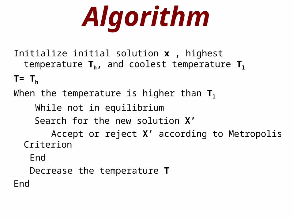
AlgorithmInitialize initial solution x , highest temperature Th, and
coolest temperature Tl
T= Th
When the temperature is higher than Tl
While not in equilibrium Search for the new solution X’
Accept or reject X’ according to Metropolis Criterion End Decrease the temperature TEnd
Simulated Annealing• Definition of solution• Search mechanism, i.e. the definition of
a neighborhood• Cost-function
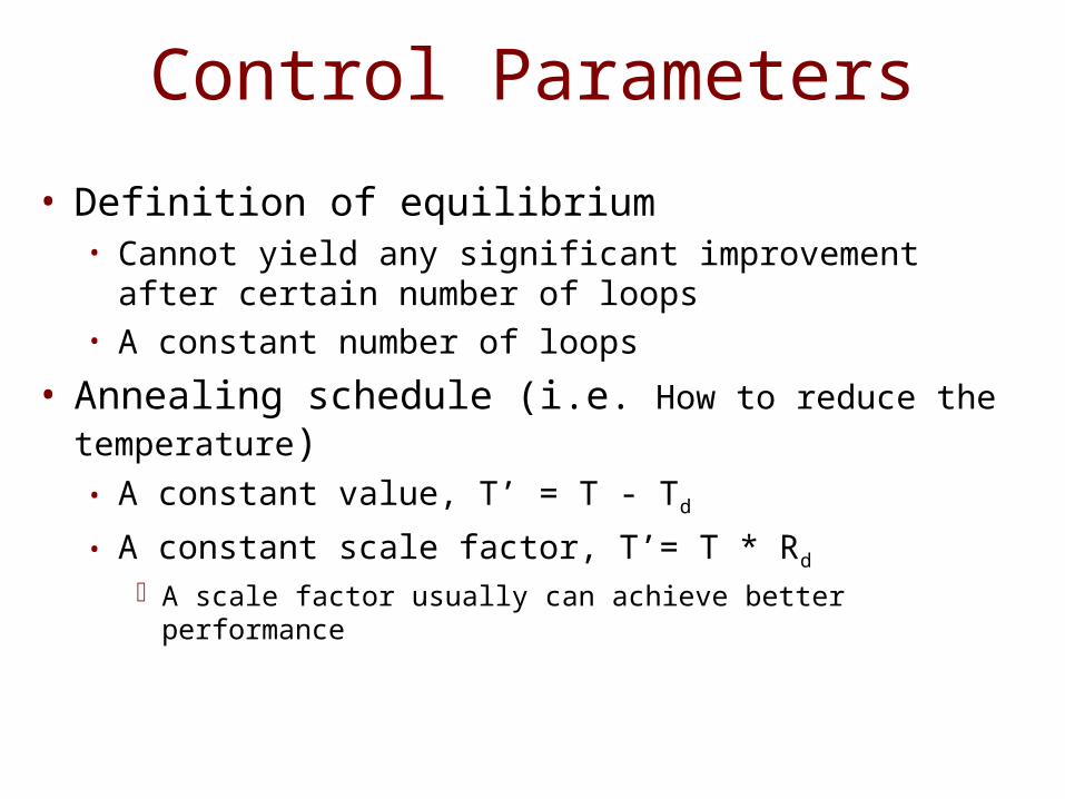
Control Parameters• Definition of equilibrium
• Cannot yield any significant improvement after certain number of loops
• A constant number of loops• Annealing schedule (i.e. How to reduce the
temperature)• A constant value, T’ = T - Td
• A constant scale factor, T’= T * RdA scale factor usually can achieve better performance
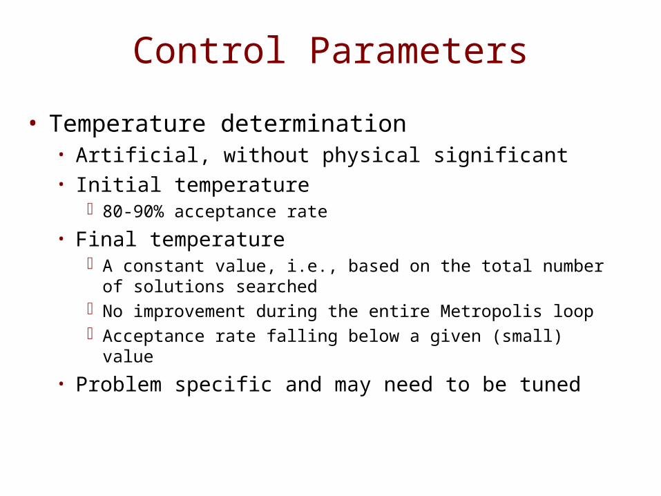
Control Parameters• Temperature determination
• Artificial, without physical significant• Initial temperature
80-90% acceptance rate• Final temperature
A constant value, i.e., based on the total number of solutions searched
No improvement during the entire Metropolis loopAcceptance rate falling below a given (small) value
• Problem specific and may need to be tuned
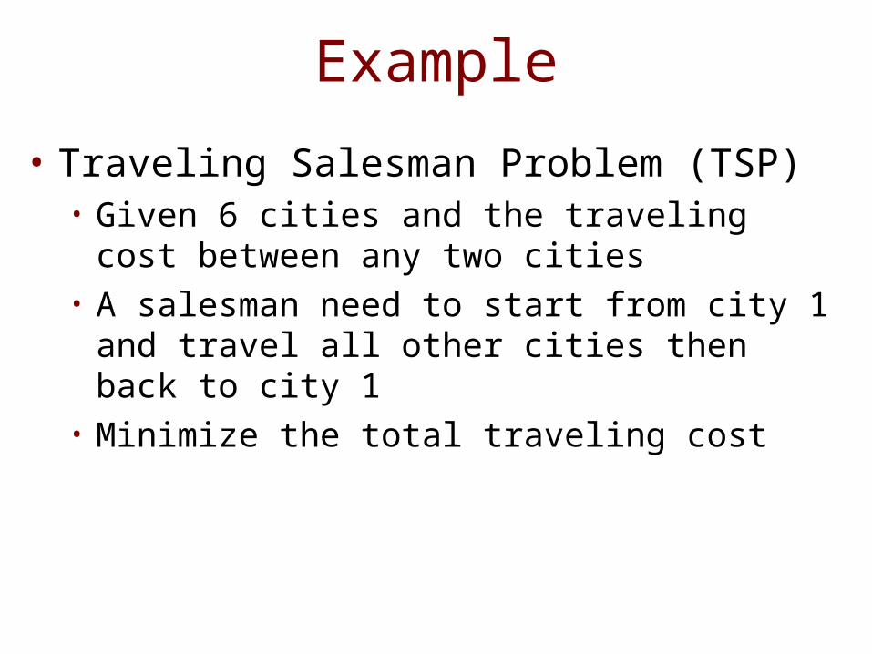
Example• Traveling Salesman Problem (TSP)
• Given 6 cities and the traveling cost between any two cities
• A salesman need to start from city 1 and travel all other cities then back to city 1
• Minimize the total traveling cost
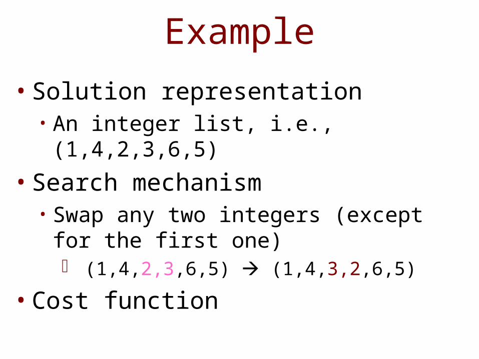
Example• Solution representation
• An integer list, i.e., (1,4,2,3,6,5)• Search mechanism
• Swap any two integers (except for the first one) (1,4,2,3,6,5) (1,4,3,2,6,5)
• Cost function
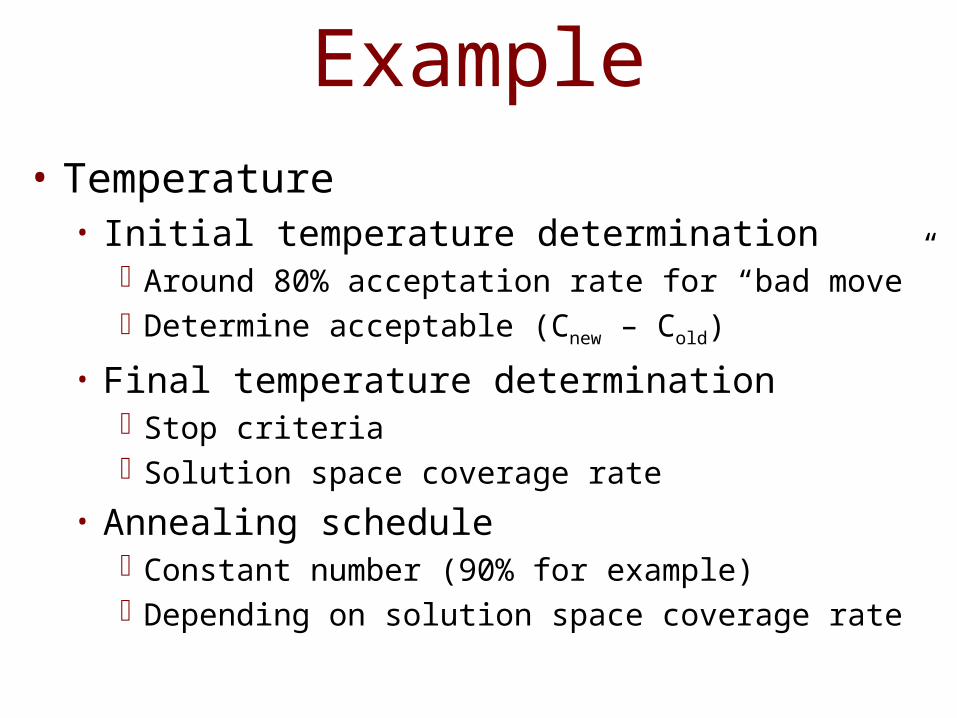
Example• Temperature
• Initial temperature determinationAround 80% acceptation rate for “bad move”Determine acceptable (Cnew – Cold)
• Final temperature determination Stop criteriaSolution space coverage rate
• Annealing scheduleConstant number (90% for example)Depending on solution space coverage rate
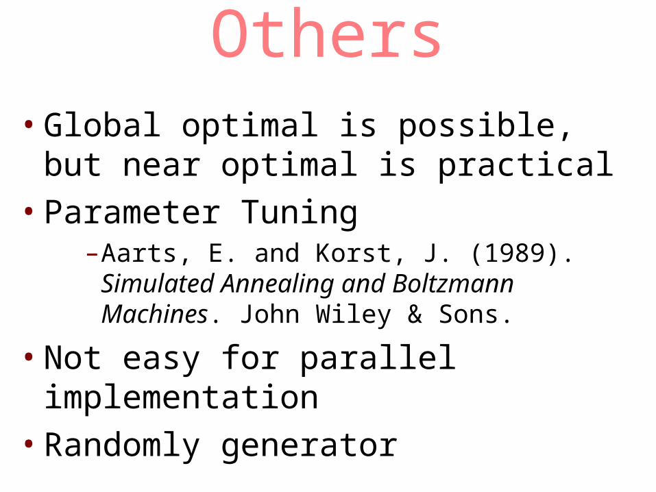
Others• Global optimal is possible, but near
optimal is practical• Parameter Tuning
–Aarts, E. and Korst, J. (1989). Simulated Annealing and Boltzmann Machines. John Wiley & Sons.
• Not easy for parallel implementation
• Randomly generator
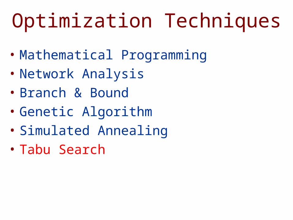
Optimization Techniques• Mathematical Programming• Network Analysis• Branch & Bound • Genetic Algorithm• Simulated Annealing• Tabu Search
Tabu Search• What
• Neighborhood search + memoryNeighborhood searchMemory
Record the search historyForbid cycling search
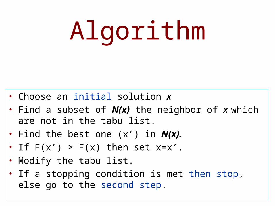
Algorithm
• Choose an initial solution X• Find a subset of N(x) the neighbor of X which are
not in the tabu list.• Find the best one (x’) in N(x).• If F(x’) > F(x) then set x=x’.• Modify the tabu list.• If a stopping condition is met then stop, else go to
the second step.
Effective Tabu Search
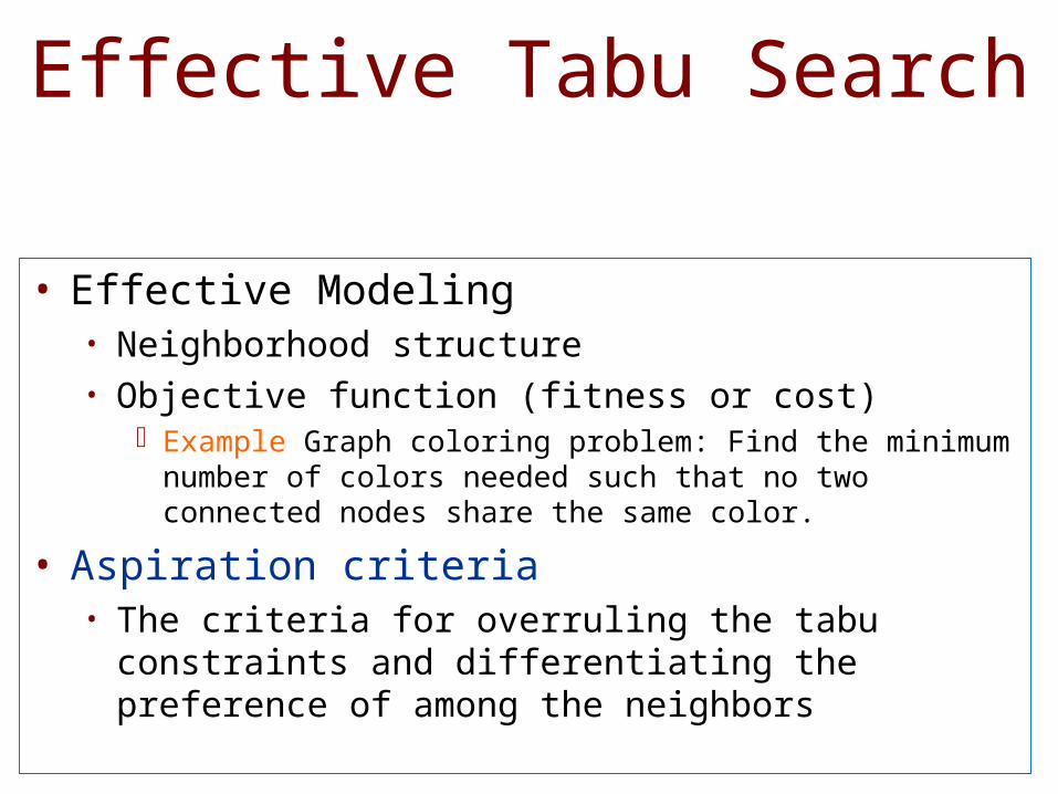
• Effective Modeling• Neighborhood structure• Objective function (fitness or cost)
Example Graph coloring problem: Find the minimum number of colors needed such that no two connected nodes share the same color.
• Aspiration criteria • The criteria for overruling the tabu constraints and
differentiating the preference of among the neighbors
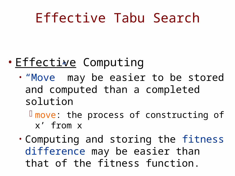
Effective Tabu Search
• Effective Computing• “Move” may be easier to be stored and
computed than a completed solution move: the process of constructing of x’
from x• Computing and storing the fitness
difference may be easier than that of the fitness function.
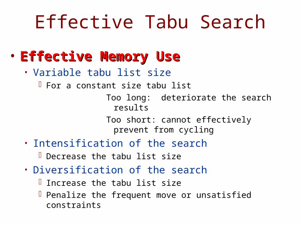
Effective Tabu Search• Effective Memory UseEffective Memory Use
• Variable tabu list sizeFor a constant size tabu list
Too long: deteriorate the search results Too short: cannot effectively prevent from
cycling• Intensification of the search
Decrease the tabu list size• Diversification of the search
Increase the tabu list sizePenalize the frequent move or unsatisfied constraints
Example• A hybrid approach for graph coloring
problem• R. Dorne and J.K. Hao, A New Genetic Local
Search Algorithm for Graph Coloring, 1998
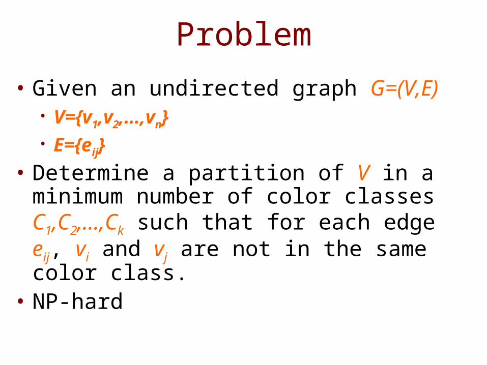
Problem• Given an undirected graph G=(V,E)
• V={v1,v2,…,vn}• E={eij}
• Determine a partition of V in a minimum number of color classes C1,C2,…,Ck such that for each edge eij, vi and vj are not in the same color class.
• NP-hard
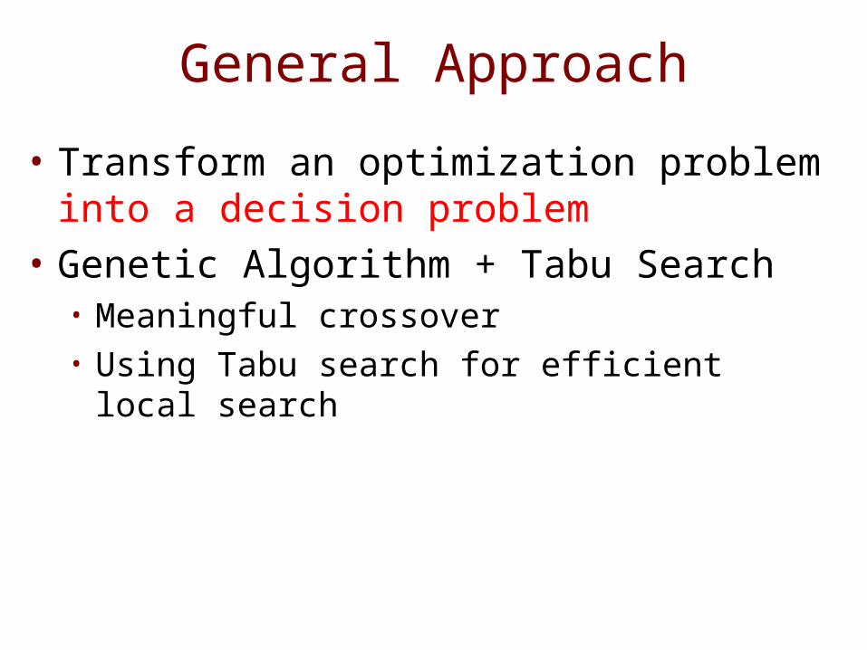
General Approach• Transform an optimization problem into
a decision problem• Genetic Algorithm + Tabu Search
• Meaningful crossover• Using Tabu search for efficient local search
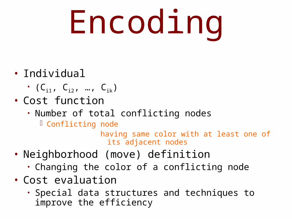
Encoding• Individual
• (Ci1, Ci2, …, Cik)• Cost function
• Number of total conflicting nodesConflicting node
having same color with at least one of its adjacent nodes
• Neighborhood (move) definition• Changing the color of a conflicting node
• Cost evaluation• Special data structures and techniques to improve the
efficiency
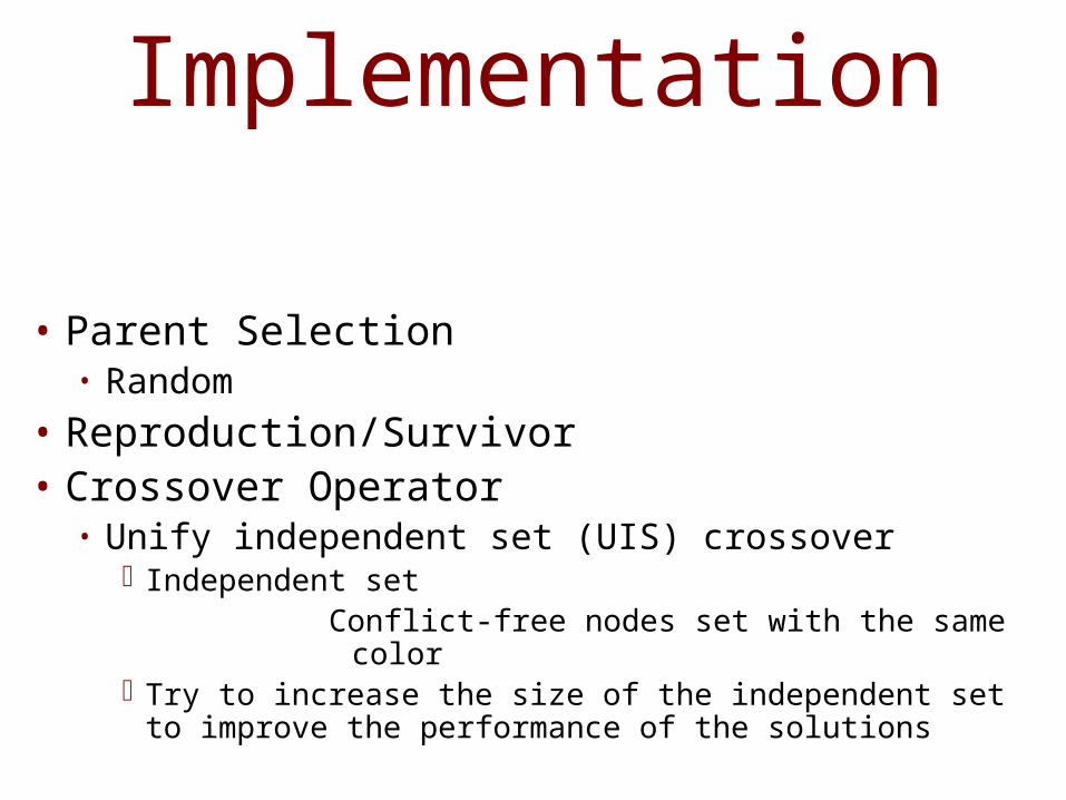
Implementation
• Parent Selection• Random
• Reproduction/Survivor• Crossover Operator
• Unify independent set (UIS) crossoverIndependent set
Conflict-free nodes set with the same color
Try to increase the size of the independent set to improve the performance of the solutions
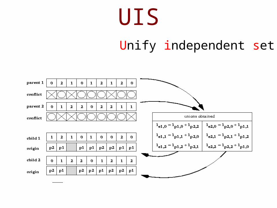
UISUnify independent set
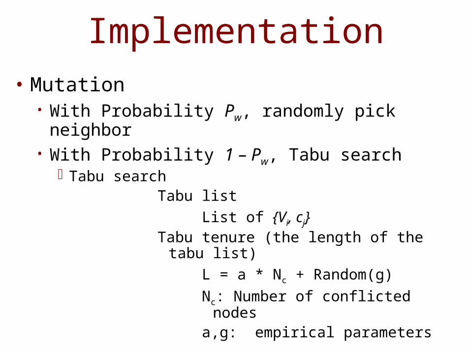
Implementation• Mutation
• With Probability Pw, randomly pick neighbor• With Probability 1 – Pw, Tabu search
Tabu searchTabu list
List of {Vi, cj}Tabu tenure (the length of the tabu
list)L = a * Nc + Random(g) Nc: Number of conflicted
nodesa,g: empirical parameters
Summary• Neighbor Search • TS prevent being trapped in the local
minimum with tabu list• TS directs the selection of neighbor• TS cannot guarantee the optimal result• Sequential• Adaptive
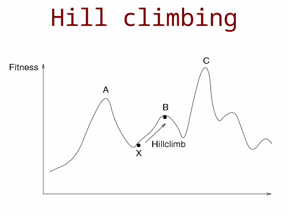
Hill climbing

sourcesJaap Hofstede, Beasly, Bull, MartinVersion 2, October 2000
Department of Computer Science & EngineeringUniversity of South Carolina
Spring, 2002