Design of a Hoverwing Aircraft

A Project

Presented to

The Faculty of the Department of

Mechanical and Aerospace Engineering

San Jose State University

In Partial Fulfillment

of the Requirements for Degree

Master of Science

In

Aerospace Engineering

By

Nita B Shah

May 2011

i

© 2011 Nita B Shah

ALL RIGHTS RESERVED San Jose State University

ii

UAbstract

Wing-in-Ground effect aircraft is one that manages level flight near the surface of the

Earth, making use of the aerodynamic interaction between the wings and the surface

known as take advantage ground effect. Ground effect is a phenomenon that relates to the

airflow around a wing when it flies in close proximity to a surface, wherein the presence

of the surface distorts the downwash from the wing and inhibits the formation of vortices.

This effect dramatically increases the lift and reduces the drag compared to that attainable

by a wing in conventional flight. The WIG crafts can transport heavy payloads at

relatively high speeds, compared to ships. Since the 1960�’s, There have been many

experiments on Wing in Ground Effect crafts and the Ekranoplan. While some believe

that it will bring a new era of high speed marine transportation, others believe it holds

less promise than the hovercraft. This paper presents a Wing-In-Ground effect craft

design as an alternative to the current ships, a means of faster and safer transportation

over water. An initial design is presented for a rigid airship that has the capacity for

16,000 lbs of payload and 2 crew members with 497 miles of range.

iv

UAcknowledgement

I would like to thank all people who have helped and inspired me during my graduate

study.

I especially want to thank my advisor, Dr. Nikos Mourtos, for his guidance during my

project and study at San Jose State University. His perpetual energy and enthusiasm in

aerospace field had motivated all his advisees, including me. In addition, he was always

accessible and willing to help his students with their research.

I was delighted to interact with Prof. Nik Djordjevic and Dr. Periklis Papadopoulos by

attending their classes and having them as my co-advisors. They deserve special thanks

as my thesis committee members and advisors.

My deepest gratitude goes to my family for their unflagging love and support throughout

my life; this dissertation is simply impossible without them. I am indebted to my parents,

Bhadresh and Meena Shah, for their care and love. As typical parents in an Indian family,

my parents worked industriously to support the family and spare no effort to provide the

best possible environment for me to grow up and attend school. They had never

complained in spite of all the hardships in their life. They uprooted their life in India and

moved to United States, so that my sister and I could have a good education and a

comfortable life. I cannot ask for more from my mother, Meena Shah, as she is simply

perfect. I have no suitable word that can fully describe her everlasting love to me. I

remember many sleepless nights with her accompanying me when I was ill. I remember

v

her constant support when I encountered difficulties and I remember, most of all, her

delicious dishes. I feel proud of my sister, Neha Shah, for her talents. She had been a role

model for me to follow unconsciously when I was a teenager and has always been one of

my best counselors. I am extremely lucky to have my fiancé, Michael Trettin, who has

supported me through some of the hardest years and I would like to take this opportunity

to thank him. He has taken many trips to San Jose State University to submit the reports

for my classes when I was not able to go. Without his support and love, I would not have

been able to come this far.

Last but not least, thanks be to God for my life through all tests in the past four years.

You have made my life more bountiful. May your name be exalted, honored, and

glorified.

vi

UTable of Contents

Abstract�…�…�…�…�…�…�…�…�…�…�…�…�…�…�…�…�…�…�…�…�…�…�…�…�…�…�….�…�…�…�….IV

Acknowledgement�…�…�…�…�…�…�…�…�…�…�…�…�…�…�…�…�…�…�…�…�…�…�…..�…�…�…�…V

Table of Contents�…�…�…�…�…�…�…�…�…�…�…�…�…�…�…�…�…�…�…�…�…�…�…�….�…�…�…VII

List of Tables�…�…�…�…�…�…�…�…�…�…�…�…�…�…�…�…�…�…�…�…�…�…�…�…�…�….�…..�…..IX

List of Figures�…�…�…�…�…�…�…�…�…�…�…�…�…�…�…�…�…�…�…�…�…�…�…�…�…�…�…�…�…X

Nomenclature�…�…�…�…�…�…�…�…�…�…�…�…�…�…�…�…�…�…�…�…�…�…�…�….�…�…�….�….XII

1. Motivation �– Mission Profile�…�…�…�…�…�…�…�…�…�…�…�…�…�…�…�…�…�…�…�…..�….....1 1.1 Motivation�…�…�…�…�…�…�…�…�…�…�…�…�…�…�…�…�…�…�…�…�…�…�…�…�…�…..1 1.2 Mission specification�…�…�…�…�…�…�…�…�…�…�…�…�…�…�…�…�…�…�…�…�…�….3

1.2.1 Mission profile�…�…�…�…�…�…�…�…�…�…�…�…�…�…�…�…�…�…�…�…�…3 1.2.2 Market analysis�…�…�…�…�…�…�…�…�…�…�…�…�…�…�…�…�…�…�…�…...4 1.2.3. Technical and economic feasibility�…�…�…�…�…�…�…�…�…�…�…�…...7 1.2.4. Critical mission requirement�…�…�…�…�…�…�…�…�…�…�…�…�…�…�….8

1.3. Comparative study of similar airplanes�…�…�…�…�…�…�…�…�…�…�…�…�…�…�…9

2. Weight Constraint Analysis�…..�…�…�…�…�…�…�…�…�…�…�…�…�…�…�…�…�…�…�…�….�…12 2.1. Database for takeoff weights and empty weights of similar airplanes�…�…...12 2.2. Determinations of regression coefficients A and B�…�…�…�…�…�…�…�…�…�…12

2.2.1 Manual calculation of mission weights�…�…�…�…�…�…�…�…�…�…�….13 2.2.2 Calculation of mission weights using the AAA program�…�…�…�….13

2.3. Takeoff weight sensitivities�…�…�…�…�…�…�…�…�…�…�…�…�…�…�…�…�…�…�…14 2.3.1. Manual calculation of takeoff weight sensitivities�…�…�…�…�…�…..14 2.3.2. Calculation of takeoff weight sensitivities using the AAA program�…�…�…�…�…�…�….16

2.4. Trade studies�…�…�…�…�…�…�…�…�…�…�…�…�…�…�…�…�…�…�…�…�…�…�…�…...17

3. Performance Constraint Analysis�…�…�…�…�…�…�…�…�…�…�…�…�…�…�…�…�…�…�…�…..20 3.1 Stall speed�…�…�…�…�…�…�…�…�…�…�…�…�…�…�…�…�…�…�…�…�…�…�…�…�…...20 3.2 Takeoff distance�…�…�…�…�…�…�…�…�…�…�…�…�…�…�…�…�…�…�…�…�…�…�….20 3.3 Landing distance�…�…�…�…�…�…�…�…�…�…�…�…�…�…�…�…�…�…�…�…�…�….�…25 3.4 Drag polar estimation�…�…�…�…�…�…�…�…�…�…�…�…�…�…�…�…�…�…�…�….�….26 3.5 Speed constraints�…�…�…�…�…�…�…�…�…�…�…�…�…�…�…�…�…�…�…�…�…�…�….29 3.6 Matching graph�…�…�…�…�…�…�…�…�…�…�…�…�…�…�…�…�…�…�…�…�…�…�…�…30

5. Fuselage Design�…�…�…�…�…�….�…�…�…�…�…�…�…�…�…�…�…�…�…�…�…�…�…�…�…�…�…32

vii

6. Wing Design�…�…�…�…�…�…�…...�…�…�…�…�…�…�…�…�…�…�…�…�…�…�…�…�…�…..�….�…34 6.1. Wing platform design�…�…�…�…�…�…�…�…�…�…�…�…�…�…�…�…�…�…�…�…�….34 6.2. Airfoil selection�…�…�…�…�…�…�…�…�…�…�…�…�…�…�…�…�…�…�…�…�…�…�…..36 6.3. Design on the lateral control surfaces�…�…�…�…�…�…�…�…�…�…�…�…�…�…�…39 6.4 CAD drawing of a wing and a winglet�…�…�…�…�…�…�…�…�…�…�…�…�…�…�…41

7. Empennage Design...�…�…�…�…�…�…�…�…�…�…�…�…�…�…�…�…�…�…�…�…�…�…�…�….�…44 7.1 Design of the Horizontal Stabilizer�….�…�…�…�…�…�…�…�…�…�…�…�…�…�…�…44 7.2 Design of the Vertical Stabilizer�…�…�…�…�…�…�…...�…�…�…�…�…�…�…�…�…..47 7.3 Empennage Design Evaluation�…�…�…�…�…�…�…�…�…�…�…�…�…�…�…�…�…�…48 7.4 Design of the Longitudinal and Directional Controls�…�…�…�…�…�…�…�…�…..51 7.5 CAD drawings�…�…�…�…�…�…�…�…�…�…�…�…�…�…�…�…�…�…�…�…�…�…�…�….51

8. Weight and Balance Analysis�…�…�…�…�…�…�…�…�…�…�…�…�…�…�…�…..�…�…�…�….�…55 8.1 Component Weight Breakdown�…�…�…�…�…�…�…�…�…�…�…�…�…�…�…�…�…..55

8.1.1 Wing Group Weight�…�…�…�…�…�…�…�…�…�…�…�…�…�…�…�….�…�…55 8.1.2 Fuselage Group Weight�…�…�…�…�…�…�…�….�…�…�…�…�…�…�….�…..55 8.1.3 Tail Group Weight�…�…�…�…�…�…�…�…�…�….�…�…�…�…�…�…�….�…..56

9. Stability and Control Analysis�…�…�…�…�…..�…�…�…�…�…�…�…�…�…�…�…�…�…�…�…�….66 9.1 Static Longitudinal Stability�…�…�…�…�…..�…�…�…�…�…�…�…�…�…�…�…�….�….66 9.2 Static Directional Stability�…�…�…�…�…..�…�…�…�…�…�…�…�…�…�…�…�…�…�….72

10. Drag Polar Calculation�…�…�…�…�…�…�…�…�…�…�…�…�…�…�…�…�…�…�…�…�…�…�…�…79 16.1 Wave Making Drag�…�…�…�…�…�…�…�…�…�…�…�…�…�…�…�…�…�…�…�…�…�…82 16.2 Drag Due to the Wetted Surface on Hull and Side Buoys�…�…�…..�…�…�…...83 16.3 Air Profile Drag�…�…�…�…�…�…�…�…�…�…�…�…�…�…�…�…�…�…�…�…�…�…�….84 16.4 Fouling Drag�…�…�…�…�…�…�…�…�…�…�…�…�…�…�…�…�…�…�…�…�…�…�….�….84

11. V-n Diagram�…�…�…�…�…�…�…�…�…�…�…�…�…�…�…�…�…�…�…�…�…�…�…�…�…�…...�….88

12. Conclusion�…�…�…�…�…�…�…�…�…�…�…�…�…�…�…�…�…�…�…�…�…�…�…�…�…�…�…�…..92

13. References�…�…�…�…�…�…�…�…�…�…�…�…�…�…�…�…�…�…�…�…�…�…�…�…�…�…�…�…...96

viii

UList of Tables

Table 1. Mission Specification 4

Table 2. Russian WIG crafts 9

Table 3. Important parameters of small scale WIG crafts 10

Table 4. Full size aircraft database of takeoff weights, empty weights and ranges 12

Table 5. Calculated results of thrust-to-weight ratio versus wing loading as a function of varied lift coefficient 21

Table 6. Calculated results of wing loading versus power loading 23

Table 7. Data for takeoff speed sizing 29

Table 8. Wing and lateral surface parameters 42

Table 9. Horizontal and vertical tail parameters 54

Table 10. Determination of preliminary component weight of the hoverwing 59

Table 11. Component weight and coordinate data 62

Table 12. Calculation of downwash gradient 71

ix

UList of Figures

Figure 1. Mission profile of hoverwing 4

Figure 2. Mission weights from AAA program 14

Figure 3. Mission fuel fractions 14

Figure 4. Results of takeoff sensitivities using AAA 16

Figure 5. Takeoff weight vs Range 17

Figure 6. Takeoff weight vs. Payload weight 17

Figure 7. Thrust-to-weight ratio vs Wing loading as a function of varied lift coefficient 22

Figure 8. Power loading vs Wing loading as a function of varied lift coefficient 24

Figure 9. AAA calculation for landing requirement 25

Figure 10. Drag polar graph 27

Figure 11. Clean drag polar 28

Figure 12. Matching results for sizing of a hoverwing 30

Figure 13. Design of the fuselage of hoverwing 33

Figure 14. Catamaran fuselage 33

Figure 15. Straight tapered wing geometry 36

Figure 16. Geometry of Clark Y airfoil 37

Figure 17. Lift coefficient vs Drag coefficient curve for Clark Y airfoil 38

Figure 18. Calculation of lift coefficient using AAA program 39

Figure 19. Geometry of a wing 41

Figure 20. Geometry of a winglet 42

x

Figure 21. Shape of NACA 4412 airfoil 46

Figure 22. Lift coefficient vs Drag coefficient for NACA 4412 airfoil 46

Figure 23. Lift coefficient vs Drag coefficient for NACA 0012 airfoil 48

Figure 24. Horizontal tail geometry tapered using AAA 48

Figure 25. Horizontal tail geometry untapered using AAA 49

Figure 26. Vertical tail geometry using AAA 49

Figure 27. Vertical tail planform using AAA 50

Figure 28. Lift coefficient for horizontal tail of the hoverwing 50

Figure 29. Lift coefficient for vertical tail of the hoverwing 51

Figure 30. Geometry of a vertical stabilizer 52

Figure 31. 3D picture of a vertical stabilizer 52

Figure 32. 3D picture of a horizontal stabilizer 53

Figure 33. Geometry of a horizontal stabilizer 53

Figure 34. Location of centre of gravity in X-direction 61

Figure 35. Location of centre of gravity in Y-direction 62

Figure 36. Center of Gravity excursion diagram 64

Figure 37. Longitudinal X-plot 66

Figure 38. Geometric parameters for horizontal tail location 69

Figure 39. Layout for computing fuselage and contribution to airplane aerodynamic center location 71

Figure 40. Directional X-plot 73

Figure 41. Effective value of vertical tail aspect ratio 74

Figure 42. Factor accounting for wing-fuselage interference

xi

with directional stability 76

Figure 43. Effect of fuselage Reynolds number on wing fuselage directional stability 77

Figure 44. Drag Polar (Boating) 85

Figure 45. Drag Polar (Planing) 85

Figure 46 Drag Polar (At takeoff, while still on water) 86

Figure 47. Drag Polar (Cruise) 86

Figure 48. Drag Polar 87

Figure 49. V-n Diagram 91

Figure 50. 3D view of hoverwing 93

Figure 51. Side view of hoverwing 93

Figure 52. Front view of hoverwing 94

Figure 53. Top view of hoverwing 94

xii

UNomenclature

Definition Symbol

g Acceleration of gravity

Cf Additional friction coefficient for roughness of the plate

A.C. Aerodynamic Center

CL Airplane lift curve slope

Air Density

g Airplane mass ratio

Da Air profile resistance

A Aspect ratio

Wstruct Airplane structural weight

WA Airframe weight

Cp Center of pressure

Cf Coefficient of water friction on a smooth plate

Cw Coefficient of wave-making

Wcrew Crew Weight

CDo Clean zero lift drag coefficient

VC Cruising speed

C.G. Centre of gravity

Vcr Cruise speed

Bc Cushion width of air channel

Pc Cushion pressure in the air channel

xiii

CD Drag Coefficient

D Drag

Dhf Drag caused by water friction of hull and sidewalls

Dswf Drag caused by water friction of sidewalls

Dihedral angle

d /d Down wash gradient

Ude Derived gust velocity

Vc Design cruising speed

Wempty Empty Weight

k Empirical constant factor

df Equivalent fuselage diameter

Cf Equivalent skin friction drag

f Equivalent parasite area

GW Flight design gross weight

V Free stream velocity

F.S. Fuselage station

Swetfus Fuselage wetted area

Df Fuselage diameter

lf Fuselage length

Wfuel Fuel Weight

Wfeq Fixed equipment weight

xiv

Dfl Fouling drag

S Gross area

Sh Horizontal size of the empennage

Vh Horizontal volume coefficient

Crh Horizontal tail root chord length

Cth Horizontal tail tip chord length

bh/2 Horizontal tail span

Ch Horizontal tail mean geometric chord

CL h Horizontal tail lift curve slope

Sweth Horizontal tail wetted area

i Incidence angle

w Kinetic viscosity coefficient

L/D Lift-to-drag ratio

nlim Limit maneuvering load factor

Mff Mission fuel fraction

Mtfo Mission trapped fuel and oil

WMZF Mission zero fuel weight

CLmaxTO Maximum take-off lift coefficient

CLmaxL Maximum landing lift coefficient

xv

VA Maneuvering speed

CNmax Maximum normal coefficient

CLmax Maximum lift coefficient

CNmaxneg Maximum negative lift coefficient

c Mean geometric chord

Vmax Maximum design speed

np Number of blades

Ncrew Number of crew

Ne Number of engines per airplane

Np Number of propellers per airplane

Npax Number of passengers

nac Number of air channels on the craft

e Oswald�’s efficiency factor

Wpayload Payload Weight

Wpwr Power plant weight

Pbl Power loading per blade

W/P Power loading

acA Position of A.C. on wing mean geometric chord

ach Position of horizontal tail on wing mean geometric chord

Swet Plan form wetted area

xvi

Mres Reserve fuel fraction

Cr Root chord

h Ratio of horizontal to wing dynamic pressure

Sa Reference area for calculating the air profile drag and lift

Vstall Stalling velocity

Cfe Skin friction coefficient

b Span

K Sweep correction factor

Clf Section lift curve slope with flaps down

Cl Section lift curve slope

c/4 Sweep angle

c/2 Semi chord sweep angle

Side slip angle

VS Stall speed

V Speed

SES Surface Effect Ship

T/W Thrust-to-Weight ratio

Wo Takeoff gross weight

T Thrust

xvii

Taper ratio

Ct Tip chord

t/c Thickness ratio

WTO Take off weight

Dt Propeller diameter

t/c Thickness ratio

TTO Tooling total take off thrust

Sv Vertical size of the empennage

Vv Vertical volume coefficient

Crv Vertical tail root chord length

Ctv Vertical tail tip chord length

bv Vertical tail span

Cv Vertical tail mean geometric chord length

CL v Vertical lift curve slope

Swetv Vertical tail wetted area

W/S Wing Loading

S Wing area

C Wing mean geometric chord

b Wing span

xviii

xix

CL w Wing lift curve slope

CL wf Wing fuselage (wing body) lift curve slope

Kwf Wing fuselage interference factor

Weng Weight per engine

W Weight

L Wetted length of hull or side buoys

Shf Wetted surface areas of the hull

Sswf Wetted surface areas of the sidewall

Chapter 1. Motivation – Mission Profile

1.1. Motivation

In recent years, the need for fast transport between and around many coastal cities has

become important for both work and recreational travel. The development of tourism has

increased the need for ferry operators, which in turn led to the discovery of new vehicle

types with higher speed and greater transport efficiency. The main reason to build a

wing-in-ground effect craft (WIG) is payload capacity and cost. WIG crafts have the

potential for payload capacities closer to fast marine crafts and the cost of construction is

much lower than aircrafts [1]. The Hoverwing can also be used in paramilitary

applications that include littoral operations, drug-running interdiction, anti-piracy, border

patrol, search and rescue, etc. In addition, the WIG crafts may be difficult to detect by

mines or sonar, making them suitable for crossing minefields and mine clearance.

WIG crafts allow for high speed marine transportation at 100 knots in comfort, without

water contact, slamming shock, stress, wake, wash or seasickness. These crafts are

extremely fuel efficient. The ability of WIG crafts to handle sea state opens the potential

usage to coastal, inter island, and major rivers. Hundreds of millions of people living and

working in these locations would benefit from WIG crafts.

WIG crafts have many benefits:

Faster travel allows for more trips, customers, and thereby more revenue

Brings new destinations closer

New routes becomes possible

1

There are benefits of zero water contact such as no sea motion or sea sickness, low

fatigue for passengers, no wash, shallow water operations. Due to these benefits, WIG

crafts would be ideal for a civilian market [1].

This project is to design a WIG craft, called Hoverwing. The idea of this craft is based on

current WIG projects taking place in Germany. Mr. Hanno Fischer has successfully

developed and tested a 2-seater WIG craft called Hoverwing 2VT. His future designs,

according to his website, include developing WIG crafts for 15, 20, and 80 passenger and

so on Hoverwing crafts. This project is to design a Hoverwing that carries 8-tons of

payload. The base parameters, such as takeoff weight, span and maximum speed, were

taken from Mr. Fischer�’s Hoverwing 80 project to initiate this project [2].

Hoverwing is a second generation WIG craft, which means that it uses static air cushion

for take-off, similar to SES and hovercrafts. A hovercraft or SES-like static air cushion is

sealed all around and air is injected into the cavity under the wing; in Hoverwing craft�’s

case, the air is sealed under the fuselage. The amount of air and the pressure of the air are

much lower than with Power Augmentation (PAR). PAR or air injection is the principle

of a jet or propeller in front of the wing that blows under the wing at take-off. The cavity

under the wing is bounded by endplates and flaps, so that the air is trapped under the

wing. This way the full weight of the WIG boat can even be lifted at zero forward speed.

The HHoverwingH uses air from the propeller that is captured by a door in the engine pylon

to power up the cushion. Some other designs propose a very low power auxiliary fan for

this purpose. This report includes the detail work of calculating important parameters

2

such as empty weight, fuel weight, drag coefficient along with developing the sizes for

wings and its control surfaces, vertical and horizontal tails, and fuselage.

1.2. Mission specification

Table 1. Mission Specification Range 497 miles

Takeoff Wave Height 5 ft

Cruising Wave Height 7 ft

Cruise altitude 15 ft Number of Crew

members 2

Payload Capacity 16,820 lbs

Number of Engines 1

Engine Type Turboprop Takeoff Field

Length 3280 ft

Landing Fiend Length 3280 ft

Cruise Speed 125 knots

1.2.1. Mission profile

The first step in designing any craft is to develop mission requirements and identify

critical requirements. For Hoverwing, the mission requirements and critical requirements

are shown in Appendices A and B. A Hoverwing starts in displacement mode at lower

speed to accelerate from stand still to its normal service speed over water. After

displacement mode, it transits from planning mode to flying mode. During transition, the

3

craft operates as a hydroplane. A hydroplane uses the water it�’s on for lift, as well as

propulsion and steering. When traveling at high speed water is forced downwards by the

bottom of the boat's HhullH. The water therefore exerts an Hequal and opposite forceH

upwards, lifting the vast majority of the hull out of the water.

Figure 1. Mission profile of hoverwing

1.2.2. Market analysis

The technology of the WIG effect craft is fairly new. A WIG craft is a high-speed

�“dynamic hovercraft�” surface/marine vehicle. Most WIG crafts have been developed

from analytical theory, model testing and building prototypes. WIG craft theory and

technology covers wide range of possible craft configurations. WIG craft size and speed

ranges from single passenger prototypes operating at 50 km/h to large military craft at

500 km/h. The largest WIG craft build to-date is KM. With a length of 348 ft and wing

4

span of 131 ft, KM is able to transport 550 tons of cargo. Due to its massive size, the KM

is also known as Caspian Sea Monster. The next vehicle in KM family was �“Orlyonok�”.

It was introduced in 1973 with 120-ton takeoff weight and AR of the main wing 3 [3].

Another type of Russian WIG craft is known as DACS, Dynamic Air Cushion Ships. The

basic element of DACS is a wing of small aspect ratio bounded by floats and rear flaps to

form a chamber. The dynamic air cushion chamber under a wing is formed by blowing of

the air with propellers mounted in front of the vehicle. For DACS, blowing air is a

permanent feature present during cruising and takeoff-touchdown modes. Though the

efficiency of DACS is similar to that of hydrofoil ships, the speed of DACS far exceeds

that of hydrofoil ships. The first practical vehicle of DACS type was the Volga-2, which

was capable of transporting 2.7 ton weight with a cruising speed of 100 to 140 km/h.

The development and design of WIG craft started in 1967 in China. In 30 years, China

has designed and tested 9 small manned WIG crafts. The XTW series were developed in

1996 by China Ship Scientific Research Center (CSSRC). Later on, 20-seat passenger

WIG effect ship was first tested in 1999. The 6-seater SDJ 1 was developed using

catamaran configuration. In 1980s, another Chinese organization, MARIC, started

developing Amphibious WIG crafts. After successfully testing 30 kg radio controlled

model, MARIC developed and tested WIG-750 with a maximum TOW of 745 kg. In

1995, the China State Shipbuilding Corporation completed AWIG-751 named, �“Swan-I�”.

It has maximum TOW of 8.1tons and cruising speed of 130 km/h. Later on, AWIG-750

was developed; it had several new features including: increased span of the main wing,

composite wing, combined use of guide vanes and flaps to enhance longitudinal stability.

5

Tests confirmed overall compliance with the design requirements, but showed some

disadvantages, such as too long shaft drives of the bow propellers, lower payload and

lower ground clearance than expected. AWIG-751G, also known as �“Swan-II�”, had

increased dimensions and an improved composite wing [3].

In 1963, Lippisch, a German aerodynamicist, introduced new WIG effect vehicle based

on the reverse delta wing planform. He built first X-112 �“Airfoil Boat�”. This and the

following Lippisch craft had a moderate aspect ratio of 3 and inverse dihedral of the main

wing enabling them to elevate the hull with respect to the water surface. The reported lift-

to-drag ratios were in order of 25. In Germany, Hanno Fischer developed his own

company �“Fischer Flugmechanik�” and extended Lippisch design concept to develop and

build a 2-seat vehicle, known as Airfish FF1/FF2. The Airfish was designed to fly only in

ground effect unlike X-112 and X-114. The Airfish was reported to have speed of 100

km/h at just half the engine�’s power during tests in 1988. Later on, the company

developed 4-seater Airfish-3. Although the craft was designed to use in ground effect, it

could perform temporary dynamic jumps climbing to a height of 4.5 m. A design series

of Airfish led to Flightship 8. The FS-8 can transport 8 people, including two crew

members. It has cruising speed of 160 km/h and a range of 365 km. The originators of

FS-8 design Fischer Flugmechanik and AFD Aerofoil Development GmbH have recently

announced a proposal to produce a new craft called hoverwing-20. The hoverwing

technology employs a simple system of retractable flexible skirts to retain an air cushion

between the catamaran of the main hull configuration. This static air cushion is used only

6

during takeoff, thus enabling the vehicle to accelerate with minimal power before making

a seamless transition to ground effect mode.

The motivation for designing the hoverwing airplane is to find a cheaper and faster

means of travel in coastal areas. The hoverwing airplanes are aimed at markets in coastal,

interisland, estuary and major rivers throughout the world, with main regions being East

Asia, the Caribbean, the Persian Gulf and the Red Sea, the Gulf of Mexico the

Mediterranean, the Baltic Sea, the Maldives and coastal Indian Ocean. Many of these

regions have a desperate need to improve transport effectiveness, which is linked to their

economic growth.

1.2.3. Technical and economic feasibility

WIG craft is about high speed marine transportation, 100 knots, in comfort, without water

contact, slamming shock, stress, wake, wash or seasickness. It is extremely fuel efficient.

The ability to handle sea state of WIG crafts open potential usage in coastal, inter island

and major rivers. Hundreds of millions of people living and working in locations these

locations would benefit from WIG craft. WIG craft is about series/mass production of

high speed marine craft at a manufacturing scale similar to the volume of the speedboat

sector [3]. The market potential for WIG craft is huge that it is worth trying hard for. Low

fuel consumption of high lift-to-drag ratio does not make WIG craft cheap. In the end,

WIG is simply about being a fast, comfortable transport solution which asks little of other

infrastructure investment. Making WIG craft commercially successful is a long journey,

but it is worth taking.

7

WIG craft is a new product, a new market and a new industry. For it to be successful the

technology must work, the Manufacturing company must be feasible, the Operating

company must be feasible. It must also mean something to the ultimate customers/users

in the civil and military markets. To an Engineer, the benefit of the WIG craft is in its

power efficiency but to an investor, the benefit of the WIG is in its ability to make profit,

which means lower operating cost. Thought WIG craft would be cheaper than an aircraft

at one point, currently that is not the case. One needs to take into account the costs of

research and development, wind tunnel testing, tank tests, safety assessment, certification

procedure, general design costs ect. If all these costs were included in the price of one

WIG, it would be more expensive than an aircraft [4]. In order to make WIG cheaper,

mass production of �“identical�” vessels must take place. In order to make money in WIG

craft, the key is to find the right market. WIG cratfs can be used to military or civil

purposes. Why is it important to find the market and what does product mean to the

market? There are benefits of zero water contact such as no sea motion or sea sickness,

low fatigue for passenger, no wash, shallow water operations. Due to these benefits, WIG

crfats would be ideal for civil market. As for the military application, though WIG crafts

have benefits, the slowness of adaption of new technology is costing military to frown

upon WIG crafts. Some day the WIG craft market is equal to the helicopter business.

According to author, Graham Taylor, demand will outstrip supply of WIG craft at least

the first decade, giving manufacturers the opportunity to pick their customer.

1.2.4. Critical mission requirement

8

A WIG craft, such as Hoverwing, need to have well-dimensioned planning surface and

high power for take-off transition. The engineers involved with WIG research have

focused on seeking methods to improve take-off performance and to reduce total installed

power. The design challenge at cruising speed is aerodynamic stability and control due to

its close proximity to the water surface.

1.3. Comparative study of similar airplanes

The mission capabilities of the similar airplanes include flying in Ground effect over

water surfaces at high speeds. WIG technology is at a very early stage and covers wide

range of craft configuration. The aircrafts listed in Table two are the Russian built

aircrafts. Some other examples of 2-seater WIGs include Hydrowing2VT, SM-9, SM-10

and Strzh. Table three shows important design parameters of small scale WIG crafts.

Table 2. Russian WIG crafts SM 6 Orlyonok KM Spasatel Volga 2

Mission

Smallexperimentalmodel ofOrlynok

TransportExperime

ntal

Guidedmissileor/and

rescue ship

Passengerboat

Maximum take offweight, t

26.42 140 544 up to 400 2.7

Payload, t 1 20 Oct up to 100 0.75

Passengermodification

150 450 8

Dimensions, L/B/Hm

31/14.8/7.85 58/31.5/1692.3/37.6

/2273.8/44/19

11.6/7.6/3.7

Lift wing, Sm 73.8 307 662.5 500 44AR, lift wing 2.81 3.07 2 3 1

9

Power plant:Starting, type and

power

2 TD9 turbojetengine, 2040 kgthrust for each

2 NK 8 4 Kfan jet

engine, 10 tthrust each

8 VD 1NM

turbojetengine,11 tthrusteach

8 NK 87turbofan

engine, 12 tthrust each

2 rotarypiston

engine, 150hp each

drving twopropellers

Cruising: type andpower

1 AI 20turboprop

engine, 4000 hp

1 NK 12 MKturbopropengine,15000hp

2 VD7KM

turbojetengine,11 tthrusteach

8 NK 87turbofan

engine, 13 rthrust

Cruising speed,km/h (knots)

290 (157)370 400(200 215)

500 (270)370 400(200 215)

120

Range, miles 497 1807.7 1242.74 2485 186

up to 1.0 1.5 5 2.5/3.5 0.5Wave height 3%

(m) Takeoff/landingCruising mode up to 1.5 no limit no limit no limit 0.3Staring distance(miles) On calm

water/ Inspecificationseastate

1.67/2.801.49

1.74/2.483.11

3.731.49

1.74/2.483.11

0.62

Starting time (s)On calm water/ In

specificationseastate

50/75 80/150 130/200 80/150 70/50

Touchdown to stop(miles), On calm

water/ Inspecificationseastate

0.75/1.12 1.67 0.75/1.05 1.92/2.80 0.75/1.05 0.50/0.62

Take off speed,knots

113.39 118.79 151.19 118.79 43.2

Table 3. Important parameters of small scale WIG crafts Development series for the Volga and Strizh

SM 9 SM 10 Volga 2 Strzh E Volga 1Build year 1977 1985 1986 1991 1998

10

1999

Length, ft 36.5 37.5 38 37.4 49Main wing span,

ft32.32 25 25 21.6 41

Tain height,ft 8.43 10.89 12.1 11.8 15.4AR, main tail 0.9 0.9 0.9 3

Crew+passengers 1+ 1+ 1+7 1+1 1+10AUW, lbs 3500 4400 5400 3260 6600

Payload, lbs 1000 2000 2000 1000Thrust, t 300 bhp 300 bhp 300 bhp 320 bhp 300 bhp

Engine stern

Engine bow2 offZMZ

4062 10

2 offZMZ

4062 10

2 offZMZ

4062 10

2 offVAS4133

2 off3M3

4062.10Maximum speed,

knots75.6 75.6 75.6 94.5 108

Cruise speed,knots

65 65 65 81 65

Range,miles n/a 186 500 311 186

11

Chapter 2. Weight Constraint Analysis

2.1. Database for takeoff weights and empty weights of similar airplanes

Table 4. Full size aircraft database of takeoff weights, empty weights and ranges Aircraft Payload weight, lbs Takeoff weight, lbs Range, mi Empty Weight, lbs

SM-6 2000 52840 800 50840

Orlyonok 40000 280000 1300 240000

KM - 1088000 2000 -

Spasatel 200000 800000 4000 600000

Volga-2 1500 5400 300 3900

SM-9 1000 3500 n/a 2500

SM-10 2000 4400 300 2500

Volga-2 2000 5400 500 3400

Strzh 1000 3260 300 2260

E-Volga-1 - 6600 300 -

Table four includes the payload weight, empty weight, takeoff weight and range of some

of the WIG crafts that has been successfully tested.

2.2. Determinations of regression coefficients A and B

According to reference [5], the regression coefficients A and B for flying boats are

0.1703 and 1.0083, respectively. The regression coefficients A and B that were found

using log-log chart were unattainable due to limited data provided for the WIG crafts.

Therefore, during the calculations of skin friction drag above values for regression

coefficients are used. The calculation of empty weight and fuel weight is shown in

section 3.3.

12

2.2.1 Manual calculation of mission weights

Step 1. The mission payload weight was assumed 16820 lbs

Step 2. The mission TOW was assumed to be 66333 lbs.

Step 3. The mission fuel weight was calculated to be 8286 lbs, with 25% fuel reserve

weight.

Step 4. WOEtent = WTOguess - WF - WPL (1)

WOEtent = 66333 �– 8286 �– 16820 = 41226 lbs.

Step 5. WEtent = WOEtent - Wtfo (2)

WEtent = 41226 lbs since crew weight is part of payload weight.

Step 6. To find WE, the following equation was used:

WE = inv log10 [(log10 WTO �– A) / B] (3)

Where the regression coefficients A and B were found to be 0.1703 and 1.0083.

B log10 WE = log10 WTO �– A

log10 WE + A = Blog10 WTO

WE = inv log10 [(log10 WTO �– A) / B] = 41033 lbs

Substituting the values of A and B into the previous equation gives us a WE of 41033 lbs

for a WTO = 66333 lbs.

Step 7. The WEtent and WE values are within the 0.5% tolerance, the calculations would

not need to be repeated.

2.2.2 Calculation of mission weights using the AAA program

13

Figure 2. Mission weights from AAA program

Figure 3. Mission fuel fractions

2.3. Takeoff weight sensitivities

2.3.1. Manual calculation of takeoff weight sensitivities

To calculate the takeoff weight the following equation was used:

10log WTO = 10logB (C WTO �– D) (4) A

where A and B were calculated in section 2.2 to be 0.1703 and 1.0083.

14

To calculate C:

C= {1 �– (1- Mres)(1 �– Mff) �– Mtfo} (5)

with Mres and Mtfo can be assumed to be zero.

To calculate D:

D = WPL + Wcrew + WPexp (6)

To calculate Mff, the following equation needed to be used:

Mff= ][7

8

6

7

5

6

4

5

3

4

2

3

2

21

WW

WW

WW

WW

WW

WW

WW

WW

TO

(7)

Mff = [0.992 + 0.990 + 0.996 + 0.985 + 0.956876 + 0.99604+0.990+0.990] = 0.900006

Therefore C = {1 �– (1- Mres)(1 �– Mff) �– Mtfo = 1 - (1 - 0.900006) = 0.900006

and D = WPL = 16820 lbs

This leads the takeoff weight to be calculated with:

10log WTO = (C WTO �– D) = 10logBA 10log1.00830.1703 (0.900006 WTO �– 16820)

WTO = WTO = 69343 lbs 16820) - (0.900006W1.0083log (0.1703 TO1010

Assuming:

WTO = 66333 lbs

WE = 41033 lbs

A = 0.1703

B = 1.0083

C = 0.90006

D = 16820

15

11010 }]/{loglog[ BAWinvBW

WW

TOTOE

TO

63.1E

TO

WW

1})1({ TOTOPL

TO WBCDBWWW

86.3PL

TO

WW

2.3.2. Calculation of takeoff weight sensitivities using the AAA program

Figure 4. Results of takeoff sensitivities using AAA

16

2.4. Trade studies

Takeoff weight vs Range

0

500

1000

1500

2000

2500

3000

3500

4000

4500

0 200000 400000 600000 800000 1000000 1200000

Takeoff Weight, WTO (lbs)

Rang

e, R

(mi)

Figure 5. Takeoff weight vs Range

Takeoff weight vs Payload weight

0

50000

100000

150000

200000

250000

0 200000 400000 600000 800000 1000000 1200000

Takeoff Weight, WTO (lbs)

Payl

oad

Wei

ght,

WPL

(lbs

)

Figure 6. Takeoff weight vs. Payload weight

17

Many of the mission weights such as the mission payload weight, take-off weight, and

fuel weight were assumed based on the design of Hoverwing 80. The WOEtent was

calculated to be 41226 lbs, which by itself seems like a reasonable weight for the WIG

craft. An empty weight of 41033 lbs was calculated with the regression coefficients from

a Reference [5]. Since the data on WIG crafts is very limited and very scattered on the

graphs, the log-log chart method was not achievable. Since the method described in

reference [5] results are within the 0.5% tolerance of the WOEtent, the calculations would

not need to be repeated.

When the mission weights were calculated in the AAA program reliable results were

obtained. The regression coefficients from reference [5] were entered and the results

showed empty weight and fuel weight to be very similar to those calculated manually.

The growth factors from AAA suggest that for every 3.82 lbs of payload weight that is

added, one pound of takeoff weight can be added. The crew growth factor is not

applicable to this project. The empty weight growth factor suggests that for every 1.63

lbs of empty weight, the takeoff weight increases by one pound. These growth factors

are encouraging because that means a higher ratio of payload to empty weight. When the

growth factors were calculated by hand, the results were with 0.5% error margin. The

empty weight sensitivity has 0% error when manually calculated.

The range of this craft is assumed to be 497 miles. According to TOP 25, endurance of

this craft has to be about 30 minutes during day time. This craft is assumed to fly only

during day time, night time endurance has not been taken into consideration. The power

required to operate this craft is higher than those listed in reference [5], therefore the

18

propeller will have be chosen. The parameter such as propeller efficiency might not be

available.

19

Chapter 3. Performance Constraint Analysis

3.1. Stall speed

An average max lift coefficient value of 1.4 was assumed. The calculations were

performed for the max weight of 66333 lbs as well as a safer goal weight of 50000 lbs.

The wing area is already known to be 3175 ft2. The density of the air at sea level is

0.00237 slugs/ft3.

W/S = 66333 / 3175 = 20.89 lb/ft2

max

5.0

2

Ls C

SW

V = 105 knots (8)

These equations were repeated for a weight of 50000 lbs, which has a wing loading W/S

= 16 lb/ft2 therefore a value of VSL = 96 knots. The lower the weight was, the lower the

stall speed. A lower stall speed is more favorable because it provides a lower landing

speed therefore a lower landing distance. This parameter is not applicable for Hoverwing

since Hoverwing will be flying very close to surface; no stalling conditions are taken into

consideration. It is calculated to estimate landing distance. Since this parameter is not

applicable for Hoverwing, AAA analysis was not taken into consideration.

3.2. Takeoff distance

The takeoff wing loading was taken as:

(W/S)TO = 66333lbs / 3175sqft = 20.89 lbs/ft2

= 1 since the pressure at sea level in ratio of pressure at sea level is very close to 1.

TOP25= (W/S)TO/{ CL MAXTO (T/W)TO} =114.7 lbs2 / ft2hp (9)

20

STOFL = 37.5 TOP25 =4304 ft

This takeoff distance was unacceptable therefore working backwards starting with a STOFL

of 3280 ft (the takeoff constraint), the takeoff parameter resulted in a value of 87.47 lbs2 /

ft2hp. The equation became:

87.47 lbs2 / ft2hp = (W/S)TO/{ CL MAXTO (T/W)TO}

By using different CLs ranging from 1.6 to 2.2, and varying the values of (W/S)TO versus

(T/W) TO , a graph was produced to see how each of the three variables affected each

other:

Table 5. Calculated results of thrust-to-weight ratio versus wing loading as a function of varied lift coefficient

CLMAXTO = 1.6 CLMAXTO= 1.8 CLMAXTO = 2.0 CLMAXTO = 2.2

(W/S)TO (T/W)TO (T/W)TO (T/W)TO (T/W)TO

5 0.03573062 0.031760551 0.028584496 0.025985905

10 0.071461239 0.063521102 0.057168992 0.05197181

15 0.107191859 0.095281653 0.085753487 0.077957716

20.89 0.149282529 0.132695581 0.119426023 0.108569112

25 0.178653099 0.158802754 0.142922479 0.129929526

30 0.214383718 0.190563305 0.171506975 0.155915431

35 0.250114338 0.222323856 0.20009147 0.181901337

40 0.285844958 0.254084407 0.228675966 0.207887242

45 0.321575577 0.285844958 0.257260462 0.233873147

50 0.357306197 0.317605509 0.285844958 0.259859052

21

0

0.05

0.1

0.15

0.2

0.25

0.3

0.35

0.4

0 10 20 30 40 50 60

Wing Loading, (W/S)TO (lb/ft2)

Thru

st-to

-Wei

ght R

atio

, (T/

W) T

O

CLMAXTO = 1.6

CLMAXTO = 1.8

CLMAXTO = 2.0

CLMAXTO = 2.2

P

Figure 7. Thrust-to-weight ratio vs Wing loading as a function of varied lift coefficient

22

By using different CDs at CL ranging from 1.6 to 2.2, and varying the values of (W/S)TO

versus (W/P) TO , a graph was produced to see how each of the 3 variables affected each

other using below equation

V = 77.3 { P (W/S)/ CD (W/P)}1/3 (10)

Using V = 125 knots, P = 0.75, and = 1, equation becomes

(W/P) = {0.000098 (W/S)}/CD

Table 6. Calculated results of wing loading versus power loading

CL = 1.6 CL = 1.8 CL = 2.0 CL = 2.2

(W/S)TO (W/P)TO (W/P)TO (W/P)TO (W/P)TO

5 0.000685 0.0004283 0.000281 0.000192305

10 0.001369 0.0008566 0.000563 0.00038461

15 0.002054 0.0012849 0.000844 0.000576915

20 0.002738 0.0017132 0.001125 0.00076922

25 0.003423 0.0021415 0.001407 0.000961525

30 0.004108 0.0025698 0.001688 0.00115383

35 0.004792 0.0029981 0.001969 0.001346135

40 0.005477 0.0034264 0.002251 0.001538441

45 0.006162 0.0038547 0.002532 0.001730746

50 0.006846 0.004283 0.002813 0.001923051

55 0.007531 0.0047113 0.003095 0.002115356

23

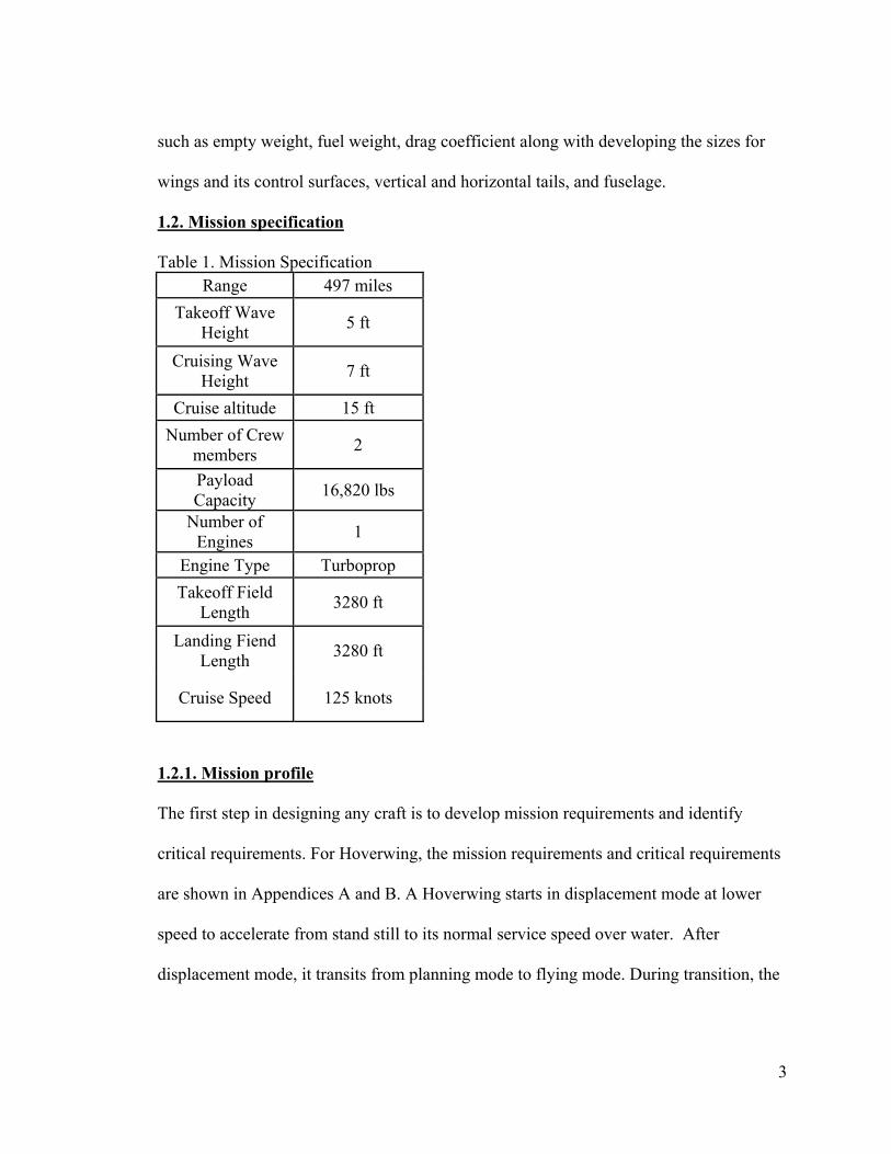
Figure 8. Power loading vs Wing loading as a function of varied lift coefficient

For Hoverwing, the CL of 1.8 was chosen. It is seen from the graph that lower CL causes

lower wing and power loadings. It is desirable to have lower wing loadings as to have

lower speeds before stall occurs. Also a lower power loading is desired so the aircraft

could have better performance. Therefore, a point should be chosen that is closest to the

lower left corner but preferably with a medium to high CL. In this case, CL of 1.8 was

chosen with wing loading of 21 to have better power loading, which gives the take off

power required to be about 6700 HP.

Power required to cruise can be found using below equation [5]:

)1(5.02

1 2

0,3

eAVSWSCVP Dreq (11)

24

Where, is 0.00237slugs/ft3, velocity is 125 knots, S is 3175 ft2, W is 66333 lb, AR is

3.45, e is 0.88 and CD,0 is 0.004. Plugging all the values in the above equation gives an

answer of 1.06 x 106 ft-lb/sec, which is about 3300 HP. According to this data,

Hoverwing will need about 3300 HP during cruise.

3.3. Landing distance

The FAR landing field length is defined as the total landing distance divided by 0.6. This

factor of safety is included to account for variations in pilot techniques and weather

conditions. It is assumed that Hoverwing will have a landing distance of 3280 ft.

VA = (SL /0.3)1/2= 88 knots (12)

VSL = VA/1.3 = 104/1.3 = 67 knots (13)

Compared to the stall speed calculated in section 2.1 of 66 knots, this value will allow us

to come to a full stop within 3280 feet.

Figure 9. AAA calculation for landing requirement

The landing distance of 3167 ft is required to have a safe landing, which is seen from

figure 8. Wing loading of 96 lb/ft2 is calculated by AAA. This data is acceptable as long

as the wing loading is under 100 lb/ft2.

25

3.4. Drag polar estimation

To calculate the drag polar ODC , the regression line coefficients for takeoff weights

versus wetted area were acquired through reference [5]. The values of c and d for flying

boats were found to be 0.6295 and 0.6708. The WTO is 66333 lbs.

10 10log logwet TOS c d W (14)

10log wetS = 3.864

To find the equivalent parasite area f, = 1.9716 was substituted into the following

equation:

10log wetS

10 10log log wetf a b S (15)

Skin friction coefficient was found using the graph 3.21c in reference [5]. The correlation

coefficients a and b were found through table 3.4 from reference [5] to be -2.3979 and 1.

f = 29.24

The equivalent parasite area and the wetted area Swet are related in the following way:3

AeCCC L

DD

2

0, (16)

where SfCD 0, (17)

By substituting the equivalent parasite area f = 29.24 into the zero-lift drag coefficient

equation:

004.00, SfCD

Substitute this information in CD equation to get following drag polar,

26

212.085.0*45.3*

4.1004.022

0, AeCCC L

DD

Low speed, clean: CD = 0.004+0.109 CL2

Clean CD

0

0.1

0.2

0.3

0.4

0.5

0.6

-3 -2 -1 0 1 2 3

Lift Coefficient, Cl

Drag

Coe

ffici

ent,

CD

Figure 10. Drag polar graph

According to figure 10, the higher the lift coefficient, the higher the drag and parasite

drag coefficients will be. It is desirable to choose a higher lift coefficient while keeping

the parasite and drag coefficients low. It is also seen that during takeoff and landing, the

drag is higher. The lift coefficient of 1.8 is chosen for Hoverwing.

27

Figure 11. Clean drag polar

28

The drag polar data from AAA were similar to data obtained by excel sheet. Since

Hoverwing will not have any lateral control surfaces or landing gear, only clean drag

calculations were made. The data achieved from AAA has similar value at Cl of 1.8,

which is 0.360. According to figure 9 and 10, the higher the lift coefficient, the higher the

drag and parasite drag coefficients will be.

In order to get the skin friction coefficient, the graph for military aircraft was chosen

from reference [5]. The aircraft that has the weight closest to Hoverwing was taken into

consideration. Therefore, the manual calculations are very reliable for drag polar.

The matching plot could not be obtained from AAA. Hoverwing does not have flaps or

slats, so when data was entered into AAA, it only produced blank graphs with no results.

0B3.5. Speed constraints Table 1 specifies a cruise speed of 125 knots at 15 ft. The low speed, clean drag polar for

the proposed airplane is given by,

CD = 0.004 + CL2/9.20, for A = 3.45 and e = 0.85

The following equation satisfies the cruise speed sizing for FAR 25 airplanes,

AeSqW

WSqC

WT OD

reqd)( (18)

By substituting the values in above equation, we get

(T/W)reqd = 4.92/(W/S) + (W/S)/9.20

Table 7. Data for takeoff speed sizing (W/S)TO (T/W)TO

15 0.18 20 0.17 25 0.16

29

30 0.15 35 0.13 40 0.12 45 0.11 50 0.10

Table 7 shows the data for cruise speed sizing for the proposed design. The ratio of thrust

at V = 125 knots at 15 ft to that sea level, static is roughly 0.1. This is based on typical

turbofan data for this type of airplane.

1B3.6. Matching graph

Figure 12. Matching results for sizing of a hoverwing

From above graph, it is seen that point P is accepted as a satisfactory match point for

Hoverwing. The airplane characteristics are summarized as follows:

Take-off weight: WTO = 66,333 lbs

30

Empty weight: WE = 41,033 lbs

Fuel weight: WF = 8286 lbs

Take-off: CL,maxTO = 1.8

Landing: CL,maxL = 1.6

Aspect ratio: 3.45

Take-off wing loading: (W/S)TO = 20.89 lb/ft2

Wing area: S = 66333/20.89 = 3175 ft2

Take-off thrust-to-weight ratio: (T/W)TO = 0.133

Take-off thrust: TTO = 8,822 lbs

31

Chapter 5. Fuselage Design

The �“Hoverwing�” will have a catamaran empennage configuration with a T-tail since it is

safer and easier to operate in water. A catamaran empennage configuration helps to build

a static air cushion by diverting some of the propeller slip-stream, which creates about

80% of the crafts weight as lift while the speed is 0. Below is the configuration of the

fuselage in exact dimensions. The configuration on the left is bottom view and the

configuration on the right is the side view. Hoverwing flies very close to surface,

therefore the cabin does not need to be pressurized. The seating arrangements are not

being discusses since this craft is designed to carry cargo only.

32

Figure 13. Design of the fuselage of hoverwing

Figure 14. Catamaran fuselage [4]

33

Chapter 6. Wing Design

6.1. Wing platform design

The wing configuration will be the conventional one as there were significant problems

with the other wing configurations, which would make the design and construction

process more difficult as well as the piloting.

The overall structural wing configuration will be a reverse delta wing. The disadvantage

of delta wing, especially in older tailless delta wing designs, are a loss of total available

lift caused by turning up the wing trailing edge or the control surfaces and the high

induces drag of this low aspect ratio type of wing. This is the reason that causes delta

winged aircraft to lose energy in turns, a disadvantage in aerial maneuver combat and

dogfighting. Since the Hoverwing will be flying very close to water surfaces, this

disadvantage will have very little to no impact in WIG craft performance.

A reverse delta will be stronger than a similar swept wing, as well as having much more

internal volume for fuel and other storage. Another advantage is that as the angle of

attack increases the leading edge of the wing generates a vortex which remains attached

to the upper surface of the wing, giving the delta a very high stall angle.

Other advantages of the delta wing are simplicity of manufacture, strength, and

substantial interior volume for fuel or other equipment. Because the delta wing is simple,

it can be made very robust. It is easy and relatively inexpensive to build. The reverse

delta wing also has a significant advantage in the longitudinal stability of the craft which

is extremely important in WIG crafts.

34

The reverse delta wing has a large aerodynamic center shift as Mach number increases

from subsonic to supersonic. This will not be a problem for Hoverwing due to expected

low speeds of the flight.

Subsonic wind-tunnel tests were conducted with a variety of leading- and trailing-edge

flap planforms to assess the longitudinal characteristics of a reverse delta wing. The

experimental data show that leading-edge flaps are highly effective at increasing

maximum lift and decreasing drag at moderate angles of attack. Trailing-edge flaps were

up to 90% as effective as delta wing flaps in generating untrimmed lift increments.

A low-wing configuration provides extreme ground effect while taking off and landing

while also providing an easier maneuvering capability during both events. It can also be

used to step out onto for hoverwing exits. Other advantages include easier access for

maintenance and cabin. Because of low-wing configuration, it provides better flexibility

on wing span yielding better cruise performance.

The wing area and the aspect ratio of the Hoverwing are 3175 ft2 and 3.45, respectively.

These values were calculated in previous reports. The taper ratio of the wing is chosen to

be 0.47 for the Hoverwing. Tapering a wing gives a higher aspect ratio, root chord to tip

chord over the span thus being more efficient. The smaller sections towards the tip

require less structure, both due to size and the reduced stress on the structure. The taper

ratio itself is usually governed by the performance expected from the plane.

The Hoverwing will have a dihedral angle of 2°. Dihedral is added to the wings to

increase the spiral stability and dutch roll stability. A major component that affects the

aircraft�’s effective dihedral is the wing location with respect to the fuselage. Having

35

dihedral also increases the ground clearance of the wings. This would be a very important

factor when flying in rough seas where waves are higher. It is seen that the dihedral

makes an aircraft more stable.

Figure 15. Straight tapered wing geometry

AAA calculated the tip chord to be 16.2 ft and root chord to be 45.6 ft, which will be

used to design the main wing. The geometry of wing could not be obtained from AAA

since AAA did not calculate for reversed delta wing. This wing configuration is very

unique; therefore AAA plot was not taken into consideration.

6.2. Airfoil selection

The Hoverwing will be fitted with a Clark Y airfoil Clark. The airfoil has a thickness of

11.7 percent and is flat on the lower surface from 30 percent of chord back. The flat

bottom simplifies angle measurements on the propellers, and makes for easy construction

of wings on a flat surface. For many applications the Clark Y has been adequate; it gives

reasonable overall performance in respect to its lift-to-drag ratio, and has gentle and

relatively benign stall characteristics. The depth of the section lends itself to easier wing

repair. The higher the lift coefficient, the more it will prevail over the effects of the drag

coefficient. Due to the expected lower velocities of flight, the effects of drag are not

36

expected to be too significant therefore increasing the benefits of a higher lift. The Cl vs

Cd curve for Clark y airfoil is shown in Figure 16. The XFLR software was unable to

calculate the curve for the Reynolds number of 1 x 107. Therefore, the Reynolds number

of 6 x 106 Lift coefficient vs Drag coefficient curve is shown in figure 17 [6].

The Hoverwing will have a 4-degree incidence angle. This helps keep the fuselage level.

It is necessary as it allows the fuselage and other components to cause as little drag as

possible. It also allows the airplane to takeoff earlier.

Figure 16. Geometry of Clark Y airfoil [6]

37

38

Figure 17. Lift coefficient vs Drag coefficient curve for Clark Y airfoil [6]

Figure 18. Calculation of lift coefficient using AAA program

When the values were entered into the AAA program, the Reynold�’s number resulted in

value of 3.2 x 107. The Cl,max values were entered in AAA program manually since the

AAA program would not calculate the Cl,max for Clark Y airfoils since it only includes the

Cl,max data for NACA airfoils.

6.3. Design on the lateral control surfaces

The Hoverwing will not have any ailerons, spoilers, flaps, slats or airbrakes. Hoverwing

is designed to fly very close to the water surface with zero to minimum amount of

turning. Therefore, there is no need to have ailerons or any other control surfaces on the

wing. The Hoverwing will have tip tanks and winglets. Wing tip tanks can act as a

winglet, store fuel at the center of gravity, and distribute weight more evenly across the

wing spar. The wingtip vortex, which rotates around from below the wing, strikes the

HcamberedH surface of the winglet, generating a force that angles inward and slightly

forward, analogous to a HsailboatH sailing Hclose hauledH. The winglet converts some of the

otherwise-wasted energy in the wingtip vortex to an apparent HthrustH. The winglets will be

15 ft in height, the root chord 21 ft, and the tip chord 8 ft. It will be located at a 56o angle

from the main wing.

39

The mean aerodynamic center (MAC) of the wing was found using by following equation

[7]:

2/

0

22 b

dyCS

MAC (19)

Since the wing of the Hoverwing is a tapered wing, the location of the MAC will be

computed using above equation. However, the chord of the tapered wing can be

calculated by below equation:

))1(21[)1(

2)( y

bbSyc w (20)

The taper ratio of the Hoverwing will be 0.47 as mentioned in section 6. From the above

equation, the chord of the wing is 32 ft. Using this value, the Reynolds number was

calculated to be 2.23 x 107. The MAC of the wing will be at ¼ chord of the MAC. The

coordinates of the MAC of the wing will be at 8 ft in from the leasing edge and 32 ft. The

Hoverwing will have reverse delta wings. Reverse delta wings have the same effect as

delta wings in terms of drag reduction, but has other advantages in terms of low-speed

handling where tip stall problems simply go away. In this case the low-speed air flows

towards the fuselage, which acts as a very large wing fence. Additionally, wings are

generally larger at the root anyway, which allows them to have better low-speed lift.

Winglets will be added to the tips of the wings as to reduce induced drag. A winglet with

a sharp corner with respect to the wing will be used, as it is easiest to construct.

Unfortunately, this choice does create problems. By being located in the pressure rise

region of the wing, winglets help move the pressure rise of the winglet behind the trailing

40

edge. Because the winglet causes a favorable pressure gradient, it cancels out some of the

wing�’s pressure rise.

6.4 CAD drawing of a wing and a winglet

Figure 19. Geometry of a wing

41

Figure 20. Geometry of a winglet

Table 8. Wing and lateral surface parameters AR 3.45

Wing area 3175 ft2

taper ratio 0.47

Re 2.31 x 107

Airfoil, root Clark Y

Airfoil, tip Clark Y

Cl 1.4

Aerodynamic

Center (x, y) (8 ft, 32 ft)

Twist angle, w �–1°

Dihedral angle, G 2°

42

LE sweep, LLE 5°

TE sweep, LTE 50°

Elevator, Ae None

Aileron, Aa None

Taper Ratio, l = ct/cr 0.47

Spoilers no

Flaps no

Leading-edge

Devices no

Winglets yes

43

Chapter 7. Empennage Design

The tilted vertical tail protects the tail wing from exposure to a downwash of the front

wing compared to a T-tail configuration. The tilted vertical tail improves product of tail

moment arm as well as the tail lift curve slope. Since the vertical tail interfere with the

fuselage and the horizontal tail, its aspect ratio increases. The local dynamic pressure is

reduced due to the converging fuselage flow going over the tail. The horizontal stabilizer

helps pull the plane�’s tail down to balance the wing C.G. moment. Though this type of

configuration is easy and safe, it is not aerodynamically efficient since the engine has to

use twice as much power to balance the plane.

By having T-tail, some aerodynamics advantages can be gained. Having mounted T-tail,

the tailplane is kept out of airflow behind the wings. By having smooth flow over the tail,

the better pitch control can be gained. T-tail is high mounted therefore; it can be out of

way of rear fuselage and this configuration is beneficial for planes that have engines in

the rear fuselage. Another advantage of having T-tail is the increased distance between

wings and tail plane since it does not have significant effect on aircraft weight. But there

are some other disadvantages of having T-tail. During deep stall, a stalled wing will block

the flow over the tail plane, resulting in total loss of pitch control. To support the forces

produced by the tail, the fin has to be made stiff and stronger which results in increasing

aircraft weight. Since the elevator surfaces are distant from the ground, it makes difficult

to check elevators from ground.

7.1. Design of the horizontal stabilizer

44

The volume method was utilized to find the surface area of the horizontal stabilizer. The

distance between the wing and tail wing was 6 ft. The equation is as follows:

L

ACVS h

HT**

(21)

Using a volume coefficient of 0.44 and the wing parameters, the area of the horizontal

stabilizer was calculated to be 668 ft2. The aspect ratio for the horizontal stabilizer was

assumed to be 2.2 based on table 8.13 in reference [7]. Using this data, the root chord of

the horizontal stabilizer was determined to be 15.9 ft and the tip chord was 9.1 ft.

The taper ratio was calculated to be 0.57 for the horizontal stabilizer. It will also have 10

of leading edge sweep.

The NACA 4412 was chosen as the airfoil design for the horizontal stabilizer. The

maximum lift coefficient of the NACA 4412 airfoil is 1.65. This parameter is very

important as the maximum lift of the wing is strongly connected to it and it is therefore

decisive for the minimum airspeed at which an aircraft can still fly horizontally. It is also

seen over the years that NACA 4412�’s characteristics with standard roughness such as

dust and bug deposits does not affect lift characteristics. It is a moderately cambered

airfoil with a nearly flat bottom. Cambering an airfoil helps provide it with a higher

maximum lift coefficient.

45

Figure 21. Shape of NACA 4412 airfoil

Figure 22. Lift coefficient vs Drag coefficient for NACA 4412 airfoil

The incidence angle of the horizontal stabilizer is assumed to be - 1 as to produce a

down force to counteract the lifting force of the main wing on the airplane. Hoverwing�’s

46

horizontal stabilizer will also have 10o of dihedral angle. It will have the taper ratio of

0.57.

7.2. Design of the vertical stabilizer

The area of the vertical stabilizer was found by the volume method with the following

equation:

SbSX

V VVV (22)

Using a volume coefficient similar to flying boats of 0.032 and the wing parameters, a

vertical tail area of 195 ft2 is calculated. The aspect ratio of the vertical stabilizer was

assumed to be 1.3 based on table 8.14 from reference [7]. Hoverwing will have two

vertical stabilizers. The area calculated above is for one vertical stabilizer. The vertical

stabilizer is recommended to be as small as possible to avoid height weathercock

stability. If an airplane is yawed due to a gust of wind, its ability to automatically return

to its previous heading depends on the area behind its center of gravity to produce a

restoring force. The fuselage ahead of the center of gravity will tend to produce a force to

destabilize the aircraft. This is called weathercock stability. Below formula is used to

calculate vertical stabilizer area:

(23)

Based on the equation above, the area of the vertical tail was calculated to be 169 ft2,

which is very close to that calculated using equations from reference [8]. The taper ratio

of our vertical stabilizer is 0.58. The vertical stabilizer will have 50o leading edge sweep.

The vertical stabilizer will have no dihedral angle and will be located 90o from the

47

horizontal tail. NACA 0012 airfoil will be used for the vertical stabilizer for simplicity

reasons. Figure 23 shows the lift coefficient curve for NACA 0012. This was calculated

using XFLR software.

Figure 23. Lift coefficient vs Drag coefficient for NACA 0012 airfoil

7.3. Empennage design evaluation

Figure 24. Horizontal tail geometry tapered using AAA

48

Figure 25. Horizontal tail geometry untapered using AAA

As seen in above figures, part of the horizontal wing is untapered, therefore, two different

calculations were run in AAA, one for tapered part and other for the untapered part. The

reason for part of the horizontal tail is untapered is so that the installment of vertical tail

to horizontal tail is easier. The planform of the horizontal tail was incorrect in AAA,

therefore it is not included.

Figure 26. Vertical tail geometry using AAA

49

Figure 27. Vertical tail planform using AAA

Figure 28. Lift coefficient for horizontal tail of the hoverwing

When the values were entered into AAA program, the Reynolds number came out to be

about in 106 range. Even though the same airfoil is being used for horizontal and vertical

tails, Reynolds number came out to be different for both tails.

50

. Figure 29. Lift coefficient for vertical tail of the hoverwing

7.4. Design of the longitudinal and directional controls

The vertical tail will have a rudder and the horizontal tail will have an elevator. The

rudder surface area will be 30% of the vertical tail area. This will provide enough force

for directional control and maneuvering. Since Hoverwing is designed to mostly fly in

straight path, the rudder and elevator will not need to be larger as they will only be used

for small directional change. The elevator will be 35% of the horizontal stabilizer area

[8]. This will provide an effective elevator authority to control the aircraft and provide

longitudinal stability.

7.5. CAD drawings

Figure 30 and 31 shows the geometry of the vertical tail and its control surfaces and

figure 32 and 33 shows the horizontal tail and its control surfaces.

51

Figure 30. Geometry of a vertical stabilizer

Figure 31. 3D picture of a vertical stabilizer

52

Figure 32. 3D picture of a Figure 33. Geometry of a horizontal stabilizer

horizontal stabilizer

53

Table 9. Horizontal and vertical tail parameters Horizontal Tail Vertical Tail

Airfoil NACA 4412 NACA 0012

CLMAX 1.5 1.3

Dihedral angle 10o None

Taper Ratio 0.57 0.58

Aspect Ratio 2.2 1.3

Sweep angle 10o 50°

Incidence Angle -1° None

Control Surfaces Elevator Rudder

Sizes of Control

Surfaces 24.10 ft x 5.6 ft 5.0 ft x 3.8 ft

54

Chapter 8. Weight and Balance Analysis

8.1. Component weight breakdown

The estimation of centre of gravity location for the airplane is calculated based on weight

break down of major components of airplane. From weight sizing calculations we have,

Gross Take off Weight, WTO = 66,333 lbs

Empty Weight, WE = 41,033 lbs

Mission Fuel Weight, WF = 8,286 lbs

Payload Weight = 16,820 lbs

Crew Weight, Wcrew = 375 lbs

Hoverwing is a water based aircraft which flies in ground effect. The Class I weight

estimation was not helpful since reference [9] did not have published data on flying

boats. The Class II Method for weight estimation of the components was used.

8.1.1. Wing group weight

The wing weight fraction, Ww /Wzf, depends upon the design limit normal maneuvering

load factor through nult =1.5nlimit. Reference [8] offers the following equation for initially

estimating the weight of the wing group

30.0

2/1

55.02/12/175.0

2/1

)cos

()]()cos3.6

(1[)cos

(0017.0MZF

ultMZFw WbSn

bbWW (24)

This equation is written for lengths in feet and weights in pounds; the quantities Wzf and

tr,max denote aircraft zero-fuel weight and wing root maximum thickness, respectively.

8.1.2. Fuselage group weight

For Hoverwing, the flying boat equation is used to calculate the fuselage weight.

55

Wf,fl.boat = 1.65Wf (25)

It is surprising that the design normal load factor does not appear in the fuselage weight

equation. It is suggested that pressure forces acting on the fuselage shell are more

significant than the fore and aft bending moments acting at the wing-fuselage juncture.

The fuselage weight is difficult to estimate because it is a complex structure with many

openings, support attachments, floors, etc., but it is strongly dependent on the gross shell

area, Sg. This is the surface area of the complete fuselage treated as an ideal surface, that

is, with no cutouts for windows or wing and tail attachments. Methods for approximating

the gross shell area are given in Appendix B in reference [8].

The fuselage weight may then be approximated by

2.12/1 )(}{02.0 fgsff

hDff S

hWlVKW (26)

In this equation the lengths are in feet, the weight is in pounds, and the design dive speed,

VD, is in knots. The length lh is the distance between the root quarter-chord points of the

tail and the wing. Above equation was also used to calculate boom weight where Wf and

hf was replaced by Wb and hb. To this basic weight, 7% should be added if the engines are

mounted on the aft fuselage.

8.1.3. Tail group weight

This group also represents a small fraction of the take-off weight, about 2% to 3%, but

that weight does have an effect on center of gravity location because of the long moment

arms. Reference [8] suggests the following functional relationships:

56

0.2,

cosh D Eh

h h h

S VW fk S

(27)

0.2,

cosv D Ev

v v v

S VW gk S

(28)

The coefficients kh and kv account for different tail configurations. For example, current

practice for airliners is to have variable incidence tails, and kh=1.1, while a fixed

horizontal stabilizer would have kh=1.0, reflecting the lighter structure typical of fixed

equipment. For fuselage-mounted vertical tails kv=1.0 while for T-tails 1 0.15 h hv

v v

S hkS b

.

In this last equation the quantities hh and bv correspond to the height of the horizontal tail

above the fuselage centerline and the height of the tip of the vertical tail above the

fuselage centerline, respectively.

]287.0)cos1000(

81.3[ 2/12/1

2.0

h

Dhhhh

VSSKW (29)

]287.0)cos1000(

81.3[ 2/12/1

2.0

h

Dvvvv

VSSKW (30)

The weight calculations of the power plant group and fixed equipment group weight

equations were obtained using below equations [11].

Commercial Transport Airplanes Engine Weight Estimation:

We = NeWeng�’ (31)

Air Induction System Weight Estimation General Aviation Airplanes Torenbeek Method:

Wai+Wp = 1.03(Ne)0.3(PTO)0.7 (32)

57

Propeller Weight Estimation Commercial Transport Airplanes Torenbeek Method:

Wprop = Kprop2(Np)0.218{DPPTO(NBl)1/2}0.782 (33)

Fuel System Weight Estimation Commercial Transport Airplanes GD Method:

For a fuel system with self-sealing bladder cells:

Wfs = 41.6{(WF/Kfps)/100}0.818+Wsupp (34)

Propulsion System Weight Estimation Commercial Transport Airplanes GD Method

Engine Controls for fuselage mounted engines

Wec = Kec(lfNe)0.792 (35)

Propulsion System Weight Estimation Commercial Transport Airplanes GD Method

Engine starting system for airplanes with turboprop engines using pneumatic starting

systems:

Wess = 12.05(We/1,000)1.458 (36)

Propulsion System Weight Estimation Commercial Transport Airplanes GD Method

Propeller Controls for turboprop engines:

Wpc = 0.322(Nbl)0.589{(NpDpPTO/Ne)/1,000}1.178 (37)

Flight Control System Weight Estimation Commercial Transport Airplanes Torenbeek

Method:

Wfc = Kfc(WTO)2/3 (38)

Hydraulic and/or Pneumatic System Weight Estimation for commercial transports:

0.0060-0.0120 of WTO

Hydraulic and/or Pneumatic System Weight Estimation Commercial Transport Airplanes

Torenbeek Method for propeller driven transports:

58

Whps+Wels = 0.325(WE)0.8 (39)

Weight Estimation For The Oxygen System Commercial Transport Airplanes Torenbeek

Method for flights below 25,000 ft:

Wox = 20+0.5Npax (40)

Auxiliary Power Unit Weight Estimation

Wapu = (0.004 to 0.013)WTO (41)

Furnishings Weight Estimation General Aviation Airplanes Torenbeek Method for single

engine airplanes:

Wfur = 5+13Npax+25Nrow (42)

Weight Estimation For Auxiliary Gear:

Waux = 0.01WE (43)

Estimating Weight of Paint

Wpt = 0.003WTO to 0.006WTO (44)

Table 10. Determination of preliminary component weight of the hoverwing Major Comp. Sub-categories W, lbs

Structure Weight, Wstruct Wing 4410

Empennage H. Tail 962.00

2 Vertical Tails V. Tail (each) 245.00

2 Booms Boom (each) 4773.00

Nacelles 689.00

Fuselage 8393.00

Power Plant Weight, Wpr Engine 2025.00

59

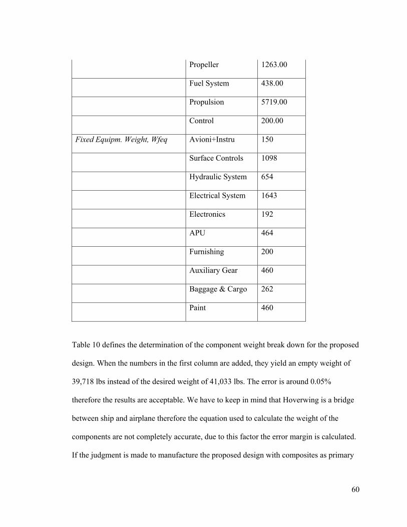
Propeller 1263.00

Fuel System 438.00

Propulsion 5719.00

Control 200.00

Fixed Equipm. Weight, Wfeq Avioni+Instru 150

Surface Controls 1098

Hydraulic System 654

Electrical System 1643

Electronics 192

APU 464

Furnishing 200

Auxiliary Gear 460

Baggage & Cargo 262

Paint 460

Table 10 defines the determination of the component weight break down for the proposed

design. When the numbers in the first column are added, they yield an empty weight of

39,718 lbs instead of the desired weight of 41,033 lbs. The error is around 0.05%

therefore the results are acceptable. We have to keep in mind that Hoverwing is a bridge

between ship and airplane therefore the equation used to calculate the weight of the

components are not completely accurate, due to this factor the error margin is calculated.

If the judgment is made to manufacture the proposed design with composites as primary

60

structural materials, significant weight savings can be obtained. A reasonable assumption

is to apply a 10% weight reduction to wing, empennage, fuselage and nacelles.

Vertical Tail

Boom

Engine

Fuselage

C.G.

Fuel

Wing

Horizontal Tail

Figure 34. Location of centre of gravity in X-direction

61

C.G.

Fuselage

Engine Boom V.T. H.T.Wing Fuel

Figure 35. Location of centre of gravity in Y-direction

Figure 34 and Figure 35 represents the Centre of gravity locations of major components

for the proposed design in X and Z directions. The X, Y, Z coordinates of each

component centre of gravity are tabulated in Table 11. The zero reference point is

considered so that all the coordinates are positive.

Table 11. Component weight and coordinate data

Major Comp. Component W xi xi + 10 Wixi yi

yi + 10 Wiyi zi

zi + 10 Wizi

Structure Weight, Wstruct Wing 4410 433.08 434.08 1914292.8 726 736 3245760 0 0 0

H. Tail 962 1223.28 1233.3 1161749.76 1256 1266 1192572 0 0 0

V. Tail 245 1199.28 1209.3 272088 1246 1256 282600 0 0 0

Boom 4773 923.28 933.28 4407881.44 650 660 3117180 0 0 0

Nacelles 689 660 670 448230 588 598 400062 0 0 0

Fuselage 8393 388.48 398.48 3322492.89 204 214 1784332 0 0 0

Power Plant Installation 9645 170 180 1724760 372 382 3660324 0 0 0

Fixed Equipment 5583 198 208 1099072 680 690 3645960 0 0 0

Fuel 8286 433.44 443.44 3674343.84 180 190 1574340 0 0 0

Payload 16820 540 550 9251000 168 178 2993960 0 0 0

WTO 66300 xcg total: 388.21 27275910.7 ycg

total: 261.4 21897090 zcg

Tot.: 0 0

62

The centre of gravity locations must be calculated for all feasible loading scenarios. The

loading scenarios depend to a large extent on the mission of the airplane. Typical loading

combinations are,

1. Empty Weight

2. Empty Weight + Fuel

3. Empty Weight + Payload + Fuel

4. Empty Weight + Crew + Fuel + Payload = Take off Weight

5. Empty Weight + Crew + Payload

As mentioned in Figure 28 and Figure 29, the centre of gravity for these loading

scenarios is calculated.

1. Weight Empty 41000 508.37

2. Empty Weight+Fuel 49826 450.98

3. Empty Weight+Payload+Fuel 66106 445.11

4. Takeoff Weight 66300 443.60

5. Empty Weight+Crew+Payload 58195 480.33

63

35000.00

40000.00

45000.00

50000.00

55000.00

60000.00

65000.00

70000.00

75000.00

425.00 450.00 475.00 500.00 525.00

Center of Gravity Location, C.G. (in)

Wei

ght,

W (l

bs)

Most aftMost fwd

WTO

WE

Empty Weight,Payload & crew

Empty Weight& Fuel

Empty Weight, Fuel& Payload

Figure 36. Center of Gravity excursion diagram

64

Figure 30 represents the C.G excursion diagram of the proposed design. The loading

sequences as well as the critical weights such as WE and WTO are determined. The C.G

locations are plotted in terms of fuselage station (F.S). From Figure 68, the most forward

C.G occurs at W = 66300 lbs, F.S = 443.60 in. and most aft C.G occurs at W = 41000 lbs,

F.S = 508.37 in.

The parametric study is performed based on the proposed mission specification by using

wing analysis program. The sweep angle for the proposed wing design is 50 , so here I

performed the study for 48 , 50 and 52 for a fixed aspect ratio and varying the taper

ratio from 0.4 to 0.6 and twist from -5 to +5 . The results from parametric study matched

to that of matching graph as discussed in section 3.6

65

Chapter 9. Stability and control analysis

9.1. Static longitudinal stability

Figure 31 represents the longitudinal X-plot. Note that the two legs of the X are

representative of,

1. The c.g leg represents the rate at which the c.g moves aft(fwd) as a function of

horizontal tail area.

2. The a.c leg represents the rate at which the a.c moves aft (fwd) as a function of

horizontal tail area [11].

Longitudinal X-Plot

0

2

4

6

8

10

12

0 100 200 300 400 500 600 700 800

Horizontal Tail Area, Sh (ft2)

Xa.

c.A

AN

D X

c.g

. (in

Xa.c. A

S.M DESIRED Xc.g Aft

Figure 37. Longitudinal X-plot

The c.g leg is calculated with the help of the class II weight and balance analysis. From

the class II weight analysis the weight of the horizontal tail is known on a per ft2 basis.

66

Assuming this quantity to be independent of surface area, the c.g can be found for any

area of the horizontal tail.

The a.c leg is calculated with the following equations:

wb

cc

hh

wb

A

L

cac

cLac

hhL

ac

ac

WhF

CSSX

ddCX

SS

ddC

XX

])}()1())(1({

[ (45)

Where

wb

cc

hh

L

cac

cLac

hhL

CSSX

ddCX

SS

ddC

F)}()1())(1({

{1[

(46)

The aerodynamic quantities can be computed with methods presented in reference [8]. As

the proposed design is a tail-aft airplane, therefore set Sc= 0 and consider Sh as the

independent variable. Both the c.g and the a.c leg of the �‘X�’ can now are plotted as a

function of area. This completes the longitudinal X-plot. The wing lift curve slope may

be estimated from the following equation.

]}4)tan1(

{2[

22/1

22/

22

22

c

L

k

AAC

w (47)

Where: SbA

2

is the wing aspect ratio

)1( 2M (48)

67

)1(

)(2M

Ck l (49)

c/2 is the semi chord sweep angle.

From wing calculations, we have

A =3.45 c/2 = 12°

M = 0.12 c/4 = 18°

By substituting the values in above equation, we get

CL w= 3.68 rad-1

The airplane lift cure slope may be estimated from,

)1)(()1)((dd

SS

Cdd

SS

CCC cccL

hhLLL chwf

(50)

Where:

CL wf is the wing fuselage (wing body) lift curve slope, given by

wwf LwfL CKC (51)

Where: Kwf is the wing fuselage interference factor given by:

2)(25.0)(025.01b

db

dK ff

wf (52)

By performing the calculations and substituting the values in wing fuselage lift curve

slope, we get

CL wf = 3.53 rad-1

68

dd

= down wash gradient at the horizontal tail which is equal to,

})(

)(]{}

21)(cos[{44.4

0

19.14/

atML

atMLchA

w

w

C

CKKKdd

(53)

Where,

)1(1)1( 7.1AA

K A (54)

7)310(K (55)

3/1)2(

)1(

bl

bh

Kh

h

h (56)

Figure 38. Geometric parameters for horizontal tail location

Based on Figure 38, the parameters for the lh and hh are calculated for the proposed

design.

69

By substituting the values in above equation, we get

d /d = 0.505

The horizontal tail lift curve slope may be estimated from below equation.

]}4)tan1(

{2[

22/1

22/

22

22

c

L

k

AAC

h (57)

By substituting the values in above equation, we get

CL h= 3.19 rad-1

CL = 3.92 rad-1

The following equation may be used to compute the location of the airplane aerodynamic

center in fractions of mean geometric chord.

L

acc

Lcach

LhLac

acC

XSS

ddCX

SS

ddCCX

Xc

ch

hwfwf

A

}]))(1())(1({)[( (58)

Where:

fwwf acacac XXX (59)

)(

)(

w

f

L

acCcSq

ddM

X (60)

13

1

2 }])(){()[08.0

)(5.36

()(i

iiif

L XddW

CqddM

i

w (61)

70

13

12

11

10

9 8

7

6

5 4

3 2

Figure 39. Layout for computing fuselage and contribution to airplane aerodynamic 1

center location

Table 12. Calculation of downwash gradient I Wf Xi d /d

1 3.2 0.978 5.7

2 4.2 1.9 8.3

3 5.6 1.2 8.3

4 6.2 0.956 7.5

5 10.2 1.1 5.6

6 28.6 1.5 12.0

71

7 24.5 1.3 8.8

8 4.9 1.1 8.1

9 4.8 1.1 8.0

10 4.8 1.3 10.6

11 4.8 1.12 10.6

12 5.0 1.15 7.10

13 5.0 0.560 7.9

By substituting the values in downwash gradient equation, we get

(dM/d ) = 9.6 * 106

By substituting these values in equation, we get

X acA

= 5.154

9.2. Static directional stability

Figure 38 shows the X-plot for static directional stability. The c.g leg is determined with

the help of class II weight analysis. The weight per ft2 of the vertical tail is known from

the weight analysis.

72

Directional X-Plot

-0.004

-0.002

0

0.002

0.004

0 100 200 300

Vertical Tail Area, SV (ft2)

Dire

ctio

nal S

tabi

lity,

C n

(deg

-1)

Figure 40. Directional X-plot

The C

n leg of the X-plot follows from:

))((b

XSSCCC vv

Lnn Vwb (62)

For twin vertical tails, the effective aspect ratio of the vertical tail may be estimated from

figure 35:

73

Figure 41. Effective value of vertical tail aspect ratio

From empennage calculations, we have

bv = 13 ft, Sv = 169 ft2

by using these values we get,

Av = 1.664

The vertical lift curve slope may be estimated from the following equation.

}]4)

tan1(

{2[

2

22/

22

22

c

veff

veffL

k

A

AC

vCL v

= 2 Aveff/ [2 + {Aveff2 2 /k2 (1+ tan2

c/2 / 2)

+4}1/2 (63)

By substituting the above calculated values in above equation, we get,

CL v= 1.69 rad-1

The fuselage contribution is calculated by,

)(3.57Sb

lSKKC ff

RNns

lf (64)

74

Where:

KN is empirical factor determined from Figure 42.

KRla factor dependent on Reynold�’s number and obtained from Figure 43.

Sfs and lf are defined in Figure 43.

75

Figure 42. Factor accounting for wing-fuselage interference with directional stability [11]

76

Figure 43. Effect of fuselage Reynolds number on wing fuselage directional stability [11]

77

By substituting these values in equation, we get

Cn = -0.038

78

Chapter 10. Drag Polar

Before we determined the drag, one needs to calculate whether the Hoverwing will sink

or float when speed is 0. In order to calculate buoyancy force, one needs to determine

water displacement, which can be calculated by below equation.

V = 35W

Buoyancy = *V

for salt water is 64 lb/ft3. Buoyancy force works out to be 73,920 lbs, while Hoverwing

weighs 66,333 lbs. If Hoverwing weighed more than 73,920 lbs, it would sink but since it

does not weigh more than 66,333 lbs, it will float.

In order to calculate zero lift drag, it is important to calculate total wetted area of the

aircraft. The wetted area of the airplane is the integral of airplane perimeter versus

distance from nose to tail. A convenient way to find the wetted area is to split the airplane

into components such as,

1. Fuselage

2. Wing

3. Empennage

4. Nacelles

5. Other contributions which contribute to wetted area

Wetted areas for Planforms

The wetted area for the proposed design is calculated by,

})1(

)1()/(25.01{2 .expr

plfwetctSS

plf (65)

79

Where = (t/c)r / (t/c)t and = ct/cr

From all the parameters obtained in section 6 and 7 and by substituting the values in

equation, we get

Swetplf

= 1296 ft2

Wetted area for fuselage

The wetted area for fuselage is calculated by,

)11()21( 266.0

ffffwet lDS

fus (66)

Where f

ff D

l

From CAD drawings, we have,

Df = 43 ft, lf = 73 ft

By substituting the values in above equation, we get

Swetfus = 3,304 ft2

Wetted area for Nacelles

The following components of the nacelle contribute to wetted area: fan cowling, gas

generator cowling and the plug. The wetted area for these components is calculated by,

)})(1(15.18.035.02{ 111

n

ef

nnn

hl

nnnwet D

Dll

DlDl

llDlS

cowlfan (67)

}])(18.01){1)(31(1[ 6.1

g

g

g

egggwet l

DDD

DlSgengas

(68)

ppwet DlSplug

7.0 (69)

80

By substituting the values in above equations, we get

Swetfancowl. = 285 ft2

Swetgas gen. = -10 ft2

Swet plug = 60 ft2

Wetted area for Horizontal tail

The wetted area for horizontal tail is calculated by,

})1(

)1()(25.01{2

r

hwetc

tSS

h (70)

From empennage calculations, we have

Sh = 630 ft2 h = 0.57

Sv = 169 ft2 v = 0.58

By substituting the values in above equation, we get

Sweth = 350 ft2

Wetted area for Vertical tail

The wetted area for vertical tail is calculated by,

})1(

)1()(25.01{2

r

vwetc

tSS

v (71)

By substituting the values in above equation, we get

Swetv = 237 ft2

Total wetted area = Swetplf

+ Swetfus + Swetfancowl. + Swetgas gen.

+ Swet plug + Sweth + Swetv �–

intersection of wing and fuselage

81

Swet = 5,250 ft2

Comparing with reference [5], shows that for transport jets with a take off weight, of

66,333 lbs the wetted area is predicted to be 5,270 ft2. This is with in the 10% expected in

the wetted area correlations.

Equivalent Parasite drag of the airplane �‘f�’

The equivalent parasite drag of the proposed airplane is f = 21 ft2.

Clean Zero �–lift drag coefficient CDo

The clean zero loft drag coefficient is calculated by,

SfC

OD

By substituting the values, we get

CDo = 0.004

The total craft drag before take-off can be expressed as follows:

D = Dhw + Dhf + Dsww + Dswf + Daw + Da+Dfl (72)

After craft take-off, the total drag can be expressed as follows:

D = Daw + Da (73)

The total drag and each separate drag component are discussed in the following.

The determination of craft drag is divided into four steps linked to the operating modes,

i.e. boating; hovering or planing before take-off; at take-off while still on water surface;

and in flying mode [12].

10.1. Wave-making drag

82

The Wave-making resistance is affected by beam to length ratio, displacement, shape of

hull, Froude number. The wave-making resistance due to air cushion pressure under the

main wings can be predicted based on Newman and Poole�’s formula as follows:

Daw = CwBcP2c (74)

Cw = f (Frc,C/Bc) (75)

Frc = V/Sqrt (gC) (76)

For approximate calculation, this can be written as:

Pc = kW/ (BcCnac) (77)

Where

k Coefficient for estimating the proportion of the weight lifted by craft air cushion on

water surface, 0.8.

Cw is calculated to be 0.0638 from above equation using weight of 66333 lbs, air cushion

channel width of 21.9 ft, and Froude number of 1.76.

10.2. Drag due to the wetted surface on hull and side buoys

The drag caused hull and side buoys can be estimated as follows:

Dhf = (Cf + Delta Cf) Shfq (78)

Dswf = (Cf + Delta Cf) Sswfq (79)

Cf = 0.075/ (logRe-2)2 (80)

Re = lsVs/ w (81)

For Reynolds number of 2.31 x 107, the skin friction drag is 0.0026. Delta Cf is additional

drag caused by roughness of the plate, which is estimated to be roughly 10-20% of Cf.

Cdhf and Cdswf is calculated to be 0.0856 and 0.00546, accordingly.

83

10.3. Air profile drag

Air profile drag can be predicted based on model experiments in wind tunnel.

Da =1/2 V2 CxSa (82)

In general, the air drag coefficient can be expressed as:

Cd,a = Cxo + K(h)C2L/ A (83)

For CL = 1.8, A = 3.45, Cxo = 0.002 which is obtained from figure in reference [14], and

K(h) = 0.2 which is obtained from reference [14], Ca is 0.0612.

10.4. Fouling drag

Since the total drag of WIG Craft is rather small compared with conventional ships, the

drag caused by the fouling is more significant, particularly during take-off, as it effects

the drag and also the lift acting on both hull and sidewall/side buoys. However, in case of

newly built craft or models, this drag component can be neglected. A factor does need to

be added for performance reduction in service; however, as the hull surfaces will never

be perfectly clean, a suggested factor is to increase the skin friction drag by 10%, which

is 0.000061.

The equations for the boating, planing before take-off, at take-off while still on water

surface and in flying mode of the proposed design are as follows:

Low speed, clean: CD = 0.004 + 0.03744 CL2

Boating: CD = 0.077 + 0.03798 CL2

Planing before take-off: CD = 0.102 + 0.03798 CL2

At take-off while still on water surface: CD = 0.222 + 0.0424 CL2

Cruise: CD = 0.125 + 0.0424 CL2

84

Drag Polar (Boating)

0

0.2

0.4

0.6

0.8

1

-6 -5 -4 -3 -2 -1 0 1 2 3

Coefficient of Lift, CL

Coe

ffici

ent o

f Dra

g, C

D

Figure 44. Drag Polar (Boating)

Drag Polar (Planing)

0

0.2

0.4

0.6

0.8

1

1.2

-6 -5 -4 -3 -2 -1 0 1 2 3 4

Coefficient of Lift, CL

Coe

ffici

ent o

f Dra

g, C

D

Figure 45. Drag Polar (Planing)

85

Drag Polar (At takeoff, while still on water)

0

0.20.4

0.6

0.8

11.2

1.4

-6 -5 -4 -3 -2 -1 0 1 2 3 4

Coefficient of Lift, CL

Coe

ffici

ent o

f Dra

g, C

D

Figure 46 Drag Polar (At takeoff, while still on water)

Drag Polar (Cruise)

0

0.2

0.4

0.6

0.8

1

1.2

-6 -5 -4 -3 -2 -1 0 1 2 3

Coefficient of Lift, CL

Coe

ffici

ent o

f Dra

g, C

D

Figure 47. Drag Polar (Cruise)

86

87

Drag Polar

00.20.40.60.8

11.21.4

-6 -4 -2 0 2 4

Coefficient of Lift, CL

Coe

ffici

ent o

f Dra

g, C

D

Drag Polar (Clean)

Drag Polar (Boating)

Drag Pola(Cruise)

Drag Polar (Planing, BeforeTake-off)Drag Polar (At take-off WhileOn Water)

Figure 48. Drag Polar

Chapter 11. V-n diagram

The V-n diagrams are used to determine design limit and design ultimate load factors as

well as the corresponding speeds to which airplane structures are designed. Figure 85

shows the V-n diagram for the proposed design. The mission specification for the

proposed aircraft is based on FAR 25 requirements. It will be assumed that under FAR 25

and will be certified under this category.

Determination of +1g stall speed: VS The design stall speed is given by,

max

)(2

NS C

SGW

V (84)

From weight sizing calculations, we have

GW = flight design gross weight in lbs = 66,333 lbs

S = wing area in ft2 = 3,175 ft2

= air density in slugs/ft3 = 0.002378 slugs/ft3

CNmax = maximum normal force coefficient

CL = 1.4

In preliminary design it is acceptable to set:

CNmax = 1.1 CLmax

By substituting the values in above equation, we get

VS = 105 kts

Determination of design cruising speed: VC

88

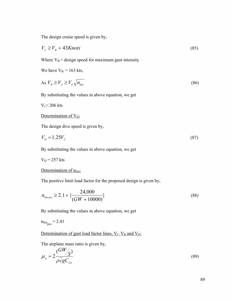
The design cruise speed is given by,

KnotsVV BC 43 (85)

Where VB = design speed for maximum gust intensity

We have VB = 163 kts,

As limnVVV SAB (86)

By substituting the values in above equation, we get

Vc= 206 kts

Determination of VD: The design dive speed is given by,

CD VV 25.1 (87)

By substituting the values in above equation, we get

VD = 257 kts

Determination of nlim: The positive limit load factor for the proposed design is given by,

})10000(

000,24{1.2lim GWn pos (88)

By substituting the values in above equation, we get

nlimpos = 2.41

Determination of gust load factor lines, VC, VB and VD: The airplane mass ratio is given by,

Lg gCc

SGW )(

2 (89)

89

By substituting the values in above equation, we get

g = 17

The gust alleviation factor is given by,

)3.5(88.0

g

ggK (90)

By substituting the values in above equation, we get

Kg = 0.67

The gust load factor is given by,

)(498

)(1lim

SGW

VCUKn Ldeg (91)

For the VC gust lines, Ude = 50 fps

For the VD gust lines, Ude = 25 fps

For the VB gust lines, Ude = 66 fps

By substituting the values in above equation, we get

nlimgust = 1 + 3.22 * 10 -3V for the VC line.

nlimgust = 1 + 1.61 * 10 -3 V for the VD line.

nlimgust = 1+ 4.25 * 10 -3 V for the VB line.

Determination of VA:

limnVV SA (92)

By substituting the values in above equation, we get

VA = 146 kts

90

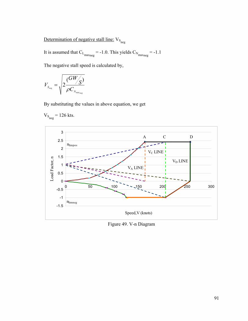
Determination of negative stall line: VSneg

It is assumed that CLmaxneg

= -1.0. This yields CNmaxneg = -1.1

The negative stall speed is calculated by,

neg

neg

NS C

SGW

Vmax

)(2

By substituting the values in above equation, we get

VSneg = 126 kts.

-1.5

-1

-0.5

0

0.5

1

1.5

2

2.5

3

0 50 100 150 200 250 300

Speed,V (knots)

Load

Fac

tor,

n

nlimpos

nlimneg

A C D

VA LINE

VC LINE

VD LINE

Figure 49. V-n Diagram

91

Chapter 12. Conclusion

The Hoverwing is a unique craft which is a mix between a ship and an airplane. As seen

from above data, the manual calculations of all the parameters are more reliable than

those obtained from AAA software. The airplanes with takeoff values closest to

Hoverwing were taken into consideration when calculation drag, horizontal and vertical

stabilizer. Though this method would not give a larger error margin, it is better than

computing in AAA software as the software compares and uses the values for airplanes

that are into certain categories such as military, jet transport, flying boat, etc. To obtain

the data, flying boats were used as a comparison. When the data for flying boats was not

available, the aircraft with similar takeoff weight was taken into consideration. The

category with similar takeoff weight was commercial transport aircraft. The weight

sensitivity results were obtained within 0.5% error margin. The CAD drawing of

Hoverwing is shown in figure 50.

92

Figure 50. 3D view of hoverwing

Figure 51. Side view of hoverwing

93

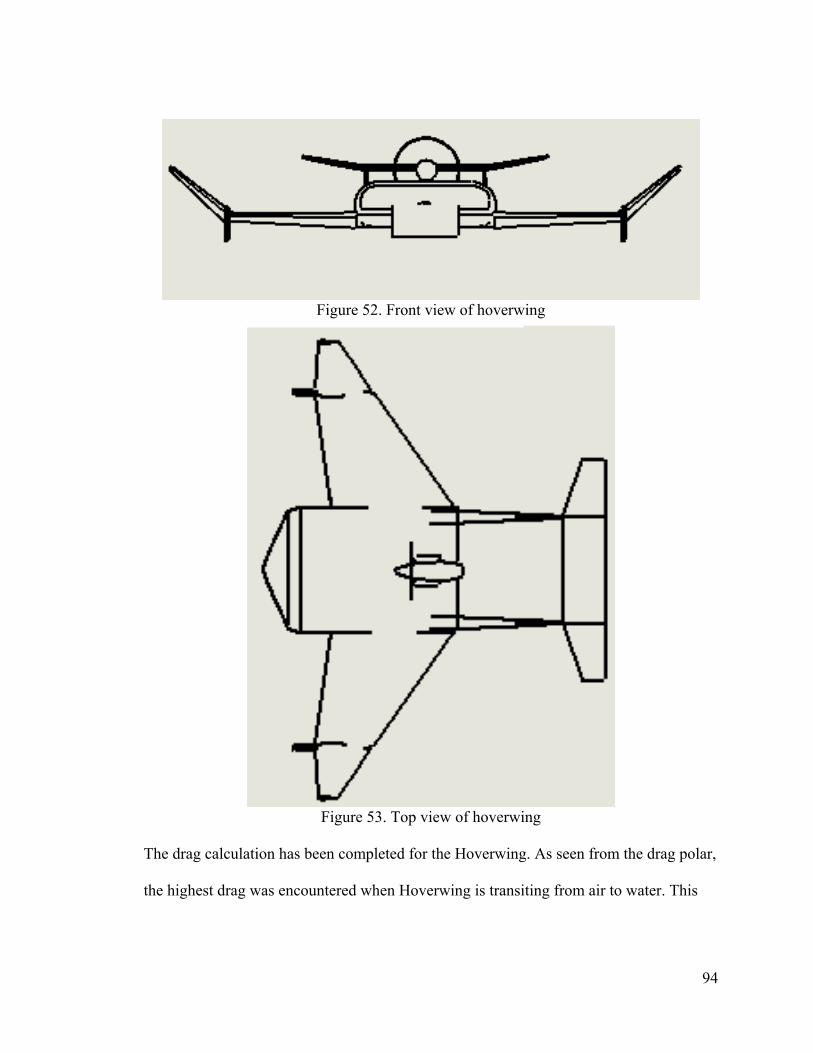
Figure 52. Front view of hoverwing

Figure 53. Top view of hoverwing

The drag calculation has been completed for the Hoverwing. As seen from the drag polar,

the highest drag was encountered when Hoverwing is transiting from air to water. This

94

data is correct since WIG crafts require more power to overcome hump speed drag.

Hoverwing will not have any landing gear as it takes off, lands and operates on water. As

seen from weight and balance analysis, Hoverwing is capable of flying in all 5 scenarios

with C.G. movement. Overall, if this design was used to produce a real craft, it would be

successful.

Hoverwing is about series/mass production of high speed marine craft at a manufacturing

scale similar to the volume of the speedboat sector. The market potential for Hoverwing

is enormous. In the end, Hoverwing is simply about being a fast, comfortable

transportation solution which requires little other infrastructure investment. Making

Hoverwing commercially successful is a long journey, but it is a venture worth exploring.

95

Chapter 13. References

[1] Taylor, G. WIG �– What Are You Waiting For? International Conference on Fast Sea

Transportation FAST�’2005, St.Petersburg, Russia, 2005.

[2] Rozhdestvensky, K. Wing-in-ground effect vehicles. 9th International Conference on

Hydrodynamics, Shanghai, China, 2010.

[3] Fischer, H., and Matjasic, K. The Hoverwing Technology-Bridge between WIG and

ACV. RTO MP-15, Amsterdam, the Netherlands, 1998.

[4] Taylor, G. The 90 Knot Zero-Wash Ferry. The Pacific 2004 International Maritime

Conference, Sydney, Australia, 2004.

[5] Roskam, Dr. Jan. Part I: Preliminary Sizing of Airplanes. DAR Corporation, Kansas,

2004.

[6] Marchman, J., and Werme, T. Clark-Y Airfoil Performance at Low Reynolds

Numbers. AIAA 22nd Aerospace Sciences Meeting, Reno, Nevada, 1984.

[7] Roskam, Dr. Jan. Part III: Layout Design of Cockpit, Fuselage, Wing and

Empennage: Cutaways and Inboard Profiles. DAR Corporation, Kansas, 2004.

[8] Torenbeek, E. Synthesis of Subsonic Airplane Design. Kluwer Academic Publishers,

Dordrecht, the Netherlands, 1982.

[9] Roskam, Dr. Jan. Part V: Component Weight Estimation. DAR Corporation, Kansas,

2004.

[10] Halloran, M. and O�’Meara, S. Wing in Ground Effect Craft Review. DSTO

Aeronautical and Maritime Research Laboratory, Melbourne, Australia, 1999.

[11] Roskam, Dr. Jan. Part VI: Preliminary Calculation of Aerodynamic, Thrust and

96

97

Power Characteristics. Airplane Design. Kansas, 2004.

[12] Yun, L., Bliault, A., and Doo, J. WIG Craft and Ekranoplan: Ground Effect Craft

Technology. Springer New York Dordrecht Heibelderg, London, 2009.