Design of a Control System for an Autonomous Vehicle …cdn.intechopen.com/pdfs/38039.pdf · International Journal of Advanced Robotic Systems Design of a Control System for an Autonomous

International Journal of Advanced Robotic Systems Design of a Control System for an Autonomous Vehicle Based on Adaptive-PID Regular Paper

Pan Zhao1,2,3, Jiajia Chen2,3, Yan Song3, Xiang Tao3, Tiejuan Xu3 and Tao Mei3,*

1 Institute of Intelligent Machines, Hefei Institutes of Physical Science, Chinese Academy of Sciences, China 2 University of Science and Technology of China, China 3 Institute of Advanced Manufacturing Technology, Hefei Institutes of Physical Science, Chinese Academy of Sciences, China * Corresponding author E-mail: [email protected] Received 10 Apr 2012; Accepted 10 May 2012 DOI: 10.5772/51314 © 2012 Zhao et al.; licensee InTech. This is an open access article distributed under the terms of the Creative Commons Attribution License (http://creativecommons.org/licenses/by/3.0), which permits unrestricted use, distribution, and reproduction in any medium, provided the original work is properly cited.

Abstract The autonomous vehicle is a mobile robot integrating multi‐sensor navigation and positioning, intelligent decision making and control technology. This paper presents the control system architecture of the autonomous vehicle, called “Intelligent Pioneer”, and the path tracking and stability of motion to effectively navigate in unknown environments is discussed. In this approach, a two degree‐of‐freedom dynamic model is developed to formulate the path‐tracking problem in state space format. For controlling the instantaneous path error, traditional controllers have difficulty in guaranteeing performance and stability over a wide range of parameter changes and disturbances. Therefore, a newly developed adaptive‐PID controller will be used. By using this approach the flexibility of the vehicle control system will be increased and achieving great advantages. Throughout, we provide examples and results from Intelligent Pioneer and the autonomous vehicle using this approach competed in the 2010 and 2011 Future Challenge of China. Intelligent Pioneer finished all of the competition programmes and won first position in 2010 and third position in 2011.

Keywords Autonomous vehicle, path‐tracking, vehicle control, adaptive‐PID control.

1. Introduction As a significant platform to show the level of artificial intelligence technology and the future of the vehicle industry, research into autonomous vehicles has become a focus of the field of robotics worldwide. An autonomous vehicle is an intelligent mobile robot which covers a set of frontier research fields including environment perception, pattern recognition, navigation and positioning, intelligent decision and control and computer science. The purpose of the research is to realize autonomous driving by the vehicle instead of human drivers and to improve traffic safety and transport efficiency. In China, a series of annual competitions called “Future Challenge of Intelligent Vehicles” has been organized by “Cognitive Computing of Visual and Auditory Information”, a Major Research Plan (MRP) of the

1Pan Zhao, Jiajia Chen, Yan Song, Xiang Tao, Tiejuan Xu and Tao Mei: Design of a Control System for an Autonomous Vehicle Based on Adaptive-PID

www.intechopen.com

ARTICLE

www.intechopen.com Int J Adv Robotic Sy, 2012, Vol. 9, 44:2012

National Nature Science Foundation of China since 2009. The third competition the 2011 Future Challenge of Intelligent Vehicles was held in Ordos city on Oct. 18, 2011 [1]. The competition took place on the urban roads in the Kangbashi district, a newly developed district with few residents. Eight teams from 10 universities attended the competition. However, only three autonomous vehicles finished the 10 km journey within the required time (50 minutes). Our intelligent vehicle named Intelligent Pioneer took 42 minutes to arrive at the finish line in second place and won the third position overall. The path‐tracking control of an autonomous vehicle is one of the most difficult automation challenges because of constraints on mobility, speed of motion, high‐speed operation, complex interaction with the environment and typically a lack of prior information. The vehicle control can be separated into lateral and longitudinal controls. Here we focus on the lateral control to follow a given trajectory with a minimum of track error. In the previous studies, various theories and methods have been investigated. These include the PID control method [2][3], the predictive control method [4], the fuzzy control method [5][6], the model reference adaptive method [7][8], the neural‐network control method [9][10], the SVR (support vector regression) method [11], the fractional‐order control method [12], etc. Recently much attention has been attracted by the use of the PID control method. PID control has such advantages as a simple structure, good control effect and robust and easy implementation [13]. Unfortunately, this method does not deal with parameter optimization and automatically adapt to the environment caused by the complexity of vehicle dynamics, uncertainty of the external environments and the non‐holonomic constraint of the vehicle[14]. To overcome these difficulties, an adaptive control algorithm has received attention and been studied. Currently adaptive control has been a great success in the industrial field [15]. The adaptive control system has the ability of adaptation, it can undertake corrective control action because of change in environments, achieving optimal or suboptimal control effects. At present the control method of adaptive control includes model reference adaptive PID control [16], fuzzy adaptive PID control [17], adaptive PID control based on neural network [18][19], adaptive PID control based on genetic algorithm [20][21] and so on. But in solving the problem of trajectory tracking of unmanned vehicles, the reference model of adaptive PID control based on the model reference is hard to ascertain because the motion model of the vehicle is influenced greatly by environments. The design of fuzzy adaptive PID control requires much priori knowledge. The vehicle finds it hard to obtain comprehensive priori knowledge when the vehicle travels in unknown environments. Adaptive PID control based

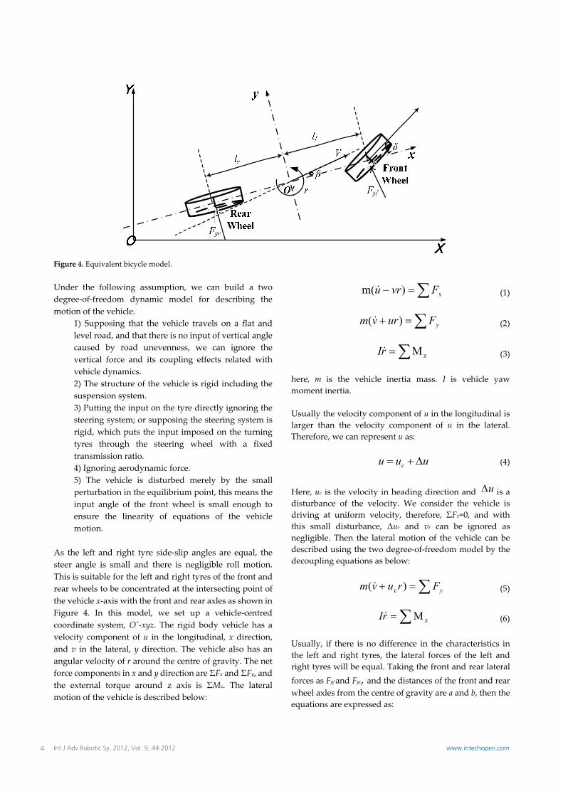
on a neural network generally use supervised learning to optimize the parameters, so it is also limited by some application conditions, for instance, the teacher signal of supervised learning is hard to obtain exactly. Although the design of adaptive PID control based on evolutionary algorithm requires less priori knowledge, it has the disadvantage of long computing times, i.e., not real time on line optimization. For the reason that we required the fluctuation of output in the control procedure caused by the disturbance to be as small as possible, namely the output of steady state equation is as small as possible, we designed the adaptive controller based on the generalized minimum variance method. The principle of this adaptive controller is simple and it is easy to realize. It can correct parameters constantly online and set the parameters of the controller constantly, so we can obtain real dynamic behaviour of the process gradually. This adaptive control method is increasingly used for industrial process control [22][23] and it is better than PID control. In this paper we describe the intelligent control system designed for an autonomous vehicle in this challenge. We first introduce briefly the system architecture used by Intelligent Pioneer, then describe the control algorithm used to generate every move of the vehicle based on the vehicle’s lateral dynamics and adaptive PID control. Then we discuss the performance of the control strategy in the simulative environment and provide results from Intelligent Pioneer in the actual test. Finally, the discussion and future work are presented. 2. System Architecture Figure 1. shows the hardware platform of Intelligent Pioneer. It is based on a 1.6L Tiggo3 SUV made by Chery Automobile Co., outfitted with two 4‐core computers and a suite of sensors. It includes four subsystems: perception system, navigation system, decision system and control system. A distributed automatic control system of the vehicle is constructed by the CAN2.0 B bus that controls objects. The state detection units can connect to each other and the control system computer can receive the information of the vehicle’s state directly using the vehicle’s body ‐ CAN. Through the CAN bus the control commands are sent to the control mechanisms, which are used to control the vehicle’s steering gear, brakes, accelerator, lights and horn respectively. The steering gear is a transformed original steering column shown in Figure 2. It realizes the accurate control of steering through a large‐power servo motor.

2 Int J Adv Robotic Sy, 2012, Vol. 9, 44:2012 www.intechopen.com

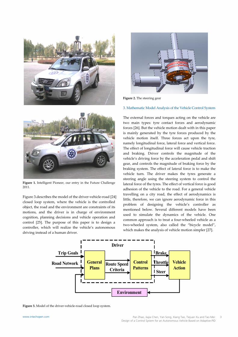
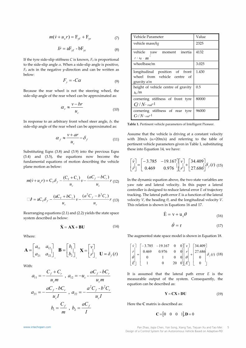
Figure 1. Intelligent Pioneer, our entry in the Future Challenge 2011. Figure 3.describes the model of the driver‐vehicle‐road [24] closed loop system, where the vehicle is the controlled object, the road and the environment are constraints of its motions, and the driver is in charge of environment cognition, planning decisions and vehicle operation and control [25]. The purpose of this paper is to design a controller, which will realize the vehicle’s autonomous driving instead of a human driver.

Figure 2. The steering gear 3. Mathematic Model Analysis of the Vehicle Control System The external forces and torques acting on the vehicle are two main types: tyre contact forces and aerodynamic forces [26]. But the vehicle motion dealt with in this paper is mainly generated by the tyre forces produced by the vehicle motion itself. Three forces act upon the tyre, namely longitudinal force, lateral force and vertical force. The effect of longitudinal force will cause vehicle traction and braking. Driver controls the magnitude of the vehicle’s driving force by the acceleration pedal and shift gear, and controls the magnitude of braking force by the braking system. The effect of lateral force is to make the vehicle turn. The driver makes the tyres generate a steering angle using the steering system to control the lateral force of the tyres. The effect of vertical force is good adhesion of the vehicle to the road. For a general vehicle travelling on a city road, the effect of aerodynamics is little, therefore, we can ignore aerodynamic force in this problem of designing the vehicle’s controller as mentioned below. Several different models have been used to simulate the dynamics of the vehicle. One common approach is to treat a four‐wheeled vehicle as a two‐wheeled system, also called the “bicycle model”, which makes the analysis of vehicle motion simpler [27].

General Plans

Road Network

Trip Goals

Route Speed Criteria

Control Patterns

Brake

Throttle

Steer

Driver

Vehicle Action

Environment

Figure 3. Model of the driver‐vehicle‐road closed loop system.


www.intechopen.com

1O

O

1

O

O

Figure 4. Equivalent bicycle model. Under the following assumption, we can build a two degree‐of‐freedom dynamic model for describing the motion of the vehicle.

1) Supposing that the vehicle travels on a flat and level road, and that there is no input of vertical angle caused by road unevenness, we can ignore the vertical force and its coupling effects related with vehicle dynamics. 2) The structure of the vehicle is rigid including the suspension system. 3) Putting the input on the tyre directly ignoring the steering system; or supposing the steering system is rigid, which puts the input imposed on the turning tyres through the steering wheel with a fixed transmission ratio. 4) Ignoring aerodynamic force. 5) The vehicle is disturbed merely by the small perturbation in the equilibrium point, this means the input angle of the front wheel is small enough to ensure the linearity of equations of the vehicle motion.

As the left and right tyre side‐slip angles are equal, the steer angle is small and there is negligible roll motion. This is suitable for the left and right tyres of the front and rear wheels to be concentrated at the intersecting point of the vehicle x‐axis with the front and rear axles as shown in Figure 4. In this model, we set up a vehicle‐centred coordinate system, Oʹ‐xyz. The rigid body vehicle has a velocity component of u in the longitudinal, x direction, and v in the lateral, y direction. The vehicle also has an angular velocity of r around the centre of gravity. The net force components in x and y direction are ΣFx and ΣFy, and the external torque around z axis is ΣMz. The lateral motion of the vehicle is described below:

xFvru )(m (1)

yFurvm )( (2)

zMrI (3)

here, m is the vehicle inertia mass. I is vehicle yaw moment inertia. Usually the velocity component of u in the longitudinal is larger than the velocity component of u in the lateral. Therefore, we can represent u as:

uuu c (4)

Here, uc is the velocity in heading direction and is a disturbance of the velocity. We consider the vehicle is driving at uniform velocity, therefore, ΣFx=0, and with this small disturbance, Δur and vr can be ignored as negligible. Then the lateral motion of the vehicle can be described using the two degree‐of‐freedom model by the decoupling equations as below:

yFruvm )( c (5)

zMrI (6)

Usually, if there is no difference in the characteristics in the left and right tyres, the lateral forces of the left and right tyres will be equal. Taking the front and rear lateral forces as Fyf and Fyr, and the distances of the front and rear wheel axles from the centre of gravity are a and b, then the equations are expressed as:

u


yryfc FF)( ruvm (7)

yryf bF-aFrI (8)

If the tyre side‐slip stiffness C is known, Fy is proportional to the side‐slip angle α. When a side‐slip angle is positive, Fy acts in the negative y‐direction and can be written as below:

-CFy (9)

Because the rear wheel is not the steering wheel, the side‐slip angle of the rear wheel can be approximated as:

cr u

brv

(10)

In response to an arbitrary front wheel steer angle, δf. the side‐slip angle of the rear wheel can be approximated as:

fc

f uarv

(11)

Substituting Eqns (3.8) and (3.9) into the previous Eqns (3.4) and (3.5), the equations now become the fundamental equations of motion describing the vehicle plane motion as below:

rubCaC

vu

ruvmc

rf

cf

)()CC(C)( rffc

(12)

ru

CbCav

ubr�I

c

rf

cf

)()CaC(aC22

rff

(13)

Rearranging equations (2.1) and (2.2) yields the state space system described as below:

BUAXX (14)

Where:

2221

1211

aaaa

A，

2

1

bb

B，

rv

X，

)(tδ fU

With:

IaC

bmC

b

IuCb-Ca

aIuCb-Ca

a

muCb-Ca

-uamuCC

a

ff

c

r2

f2

c

rf

c

rfc

c

rf

21

2221

1211

，

，

，

Vehicle Parameter Value

vehicle mass/kg 2325

vehicle yaw moment inertia mkgI

2/

4132

wheelbase/m 3.025

longitudinal position of front wheel from vehicle centre of gravity a/m

1.430

height of vehicle centre of gravity gh /m

0.5

cornering stiffness of front tyre radNCf 1/

80000

cornering stiffness of rear tyre radNCr 1/

96000

Table 1. Pertinent vehicle parameters of Intelligent Pioneer. Assume that the vehicle is driving at a constant velocity with 20m/s (uc=20m/s) and referring to the table of pertinent vehicle parameters given in Table 1, substituting these into Equation 14, we have:

)(686.27409.34

976.0469.0167.19785.3

trv

rv

f

(15)

In the dynamic equation above, the two state variables are yaw rate and lateral velocity. In this paper a lateral controller is designed to reduce lateral error E of trajectory tracking. The lateral path error E is a function of the lateral velocity V, the heading θ, and the longitudinal velocity V. This relation is shown in Equations 16 and 17.

cuvE (16)

r (17)

The augmented state space model is shown in Equation 18.

)(

00686.27409.34

02001001000976.0469.000167.19785.3

t

E

rv

E

rv

f

(18)

It is assumed that the lateral path error E is the measurable output of the system. Consequently, the equation can be described as:

DUCXY (19)

Here the C matrix is described as:

0,1000 DC


www.intechopen.com

The lateral path error E is also the quantity which must be controlled. This system’s open‐loop control transfer function of interest is thus the transfer function from steering angle input to path error output. This may be determined using Equation 20.

234

2

s5.295 + s2.809 + s2419 + s10.52 - s34.41

ssG

DBAIC 1)()(

(20)

Note that the relative degree is 2, the numerator is Hurwitz, the denominator has a double root at the origin and the sign of the high frequency gain is known (positive). Now that the structure of the plant is known, the next section describes the design of a model reference adaptive controller for controlling the lateral path error. 4. Controller Design Based on Adaptive PID In the design of the controller, the study is based on the performance index of these:

(1) Settling time less than 2s, within 1% of final value;

(2) Overshot of step responsive less than 10%; (3) Steady‐state error of step responsive is 0.

Equation 20can be written as below:

)(1 5.295+s 2.809 + s

2419 + s 10.52 - s 34.411)(G 22

2

2 sCss

s (21)

Because 0 is the double pole of the system, the system will be unstable. We must use velocity feedback, see as Figure 5.

( )y t( )f t T

Figure 5. Closed‐loop control strategy. Figure 6 shows the structure of the control strategy used. It is simulated using MATLAB. The coefficient is chosen at K=10 to make the additional zero point nearby the origin, therefore,

)101()( ssH . The system’s open‐loop transfer function becomes:

5.295) +s 2.809 + (ss2419) + s 10.52 - s 10s)(34.41(1)()()1( 22

2

2

sHsC

s (22)

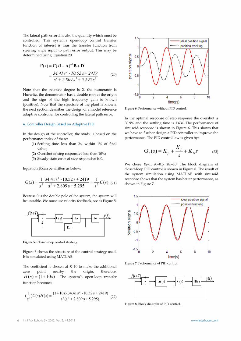
Figure 6. Performance without PID control. In the optimal response of step response the overshot is 30.9% and the settling time is 1.63s. The performance of sinusoid response is shown in Figure 6. This shows that we have to further design a PID controller to improve the performance. The PID control law is given by:

sKs

KKs DI

p )(Gc

(23)

We chose Kp=1, KI=0.5, KD=10. The block diagram of closed‐loop PID control is shown in Figure 8. The result of the system simulation using MATLAB with sinusoid response shows that the system has better performance, as shown in Figure 7.

Figure 7. Performance of PID control.

( )y t( )f t T

Figure 8. Block diagram of PID control.


The above analysis is just a preliminary approach under ideal dynamics models, but we have ignored many factors which make automatic lateral control of vehicles difficult. These include changing vehicle parameters with time, changing road conditions, as well as disturbances caused by GPS signal attenuation and other factors. Traditional controllers have difficulty in guaranteeing performance and stability over a wide range of parameter changes. In order to solve these problems and make the system automatically adapt to changes of the environment and parameters, we designed an adaptive PID controller. The requirement of the adaptive PID control is control of the system’s internal parameters independent of a precise mathematic model and that the parameters can adjust automatically online by real‐time performance requirements. The adaptive PID control combines with the advantages of adaptive control and conventional PID control. Using an adaptive PID controller, the PID parameters can be changed with the state of control object to obtain better control performance. In this paper we have established a single input single output control system. We describe the control object using the controlled auto regressive model as:

)()()()()( ttuzBztyzA d (24)

Where , and )(t are system output, input and zero mean white noise sequence. d is pure delay of system. A(z) and B(z) are

a

a

nn zazazazazA 3

32

21

11 1)(

b

b

nn zbzbzbzbzB 3

32

21

11 1)(

We propose a control strategy based on minimum variance [28]. This means that the output variance of the control system must be a minimum, so it can improve the smoothness and give a comfortable ride during the vehicle’s movement. The performance index function is defined as:

min)}({ 2 tyEJ (25)

According to Diophantine equation [29], there are polynomials D(z) and E(z) that make J minimize. Thus, the control law is:

)()()()()()( 11

1

zDzBtyzEtrtu

(26)

We ignore the disturbances of higher order term in the system and set E(z) as a two order polynomial, as below:

21 )2()1()()( zkezkekezE (27)

To ensure that the system has a zero steady‐state error after any disturbance, we chose:

)2()1()()(1

kekekezEz

(28)

According to generalized minimum variance law, an adaptive PID controller can be described as:

)2()2()1()1()())2()1()((

)()1()( 01

0

kykkekykkekrkekekek

kuzku

(29)

And the control equation of ordinary PID controller is:

]d)(dd)(1)([)(

0 t

di

p tteTtte

TteKtu

(30)

Here Kp, Ti and Td are proportional gain, integration time constant and derivative time constant, and e(t) is the lateral path error which we need to control. If we take Ts as the sampling period, the controller equation can be discretized as below:

))]1()(()()([)(1

kekeTTje

TTkeKku

t

j s

d

i

sp

(31)

Then transform Equation 31 as the incremental form:

)2()1()21(

)()1()()(

kyTTKky

TTK

kyTT

TTKkr

TTK

ku

s

dp

s

dp

s

d

i

sp

i

sp

(32)

Comparing the two Equations 29 and 32, the control parameters can be deduced as:

))2(2)1(( kekekK p (33)

)2()1()())2(2)1((

kekekeTkekeT s

i

(34)

)2(2)1()2(

kekeTkeT s

d

(35)

Where, Ts is the control period which in our control system is 0.1s. The parameters k and Kp play similar control roles. That means the system has a low damping response when k is bigger. Conversely, the system has a high damping response when k is smaller.


www.intechopen.com

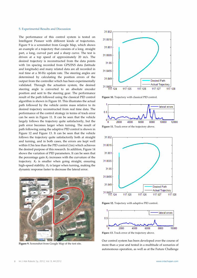
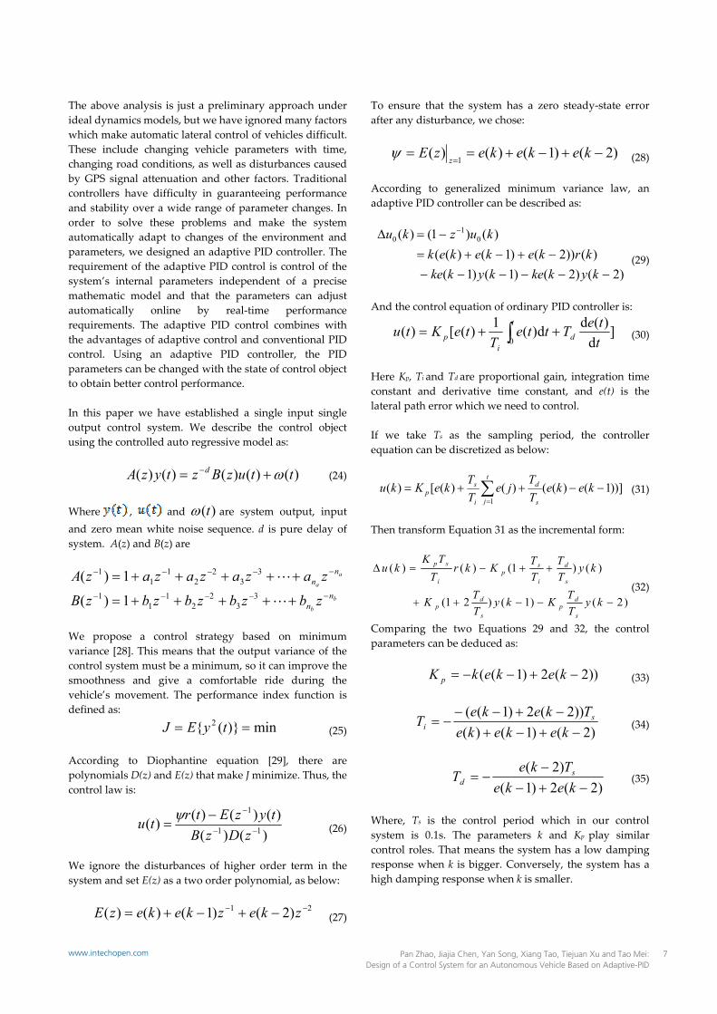
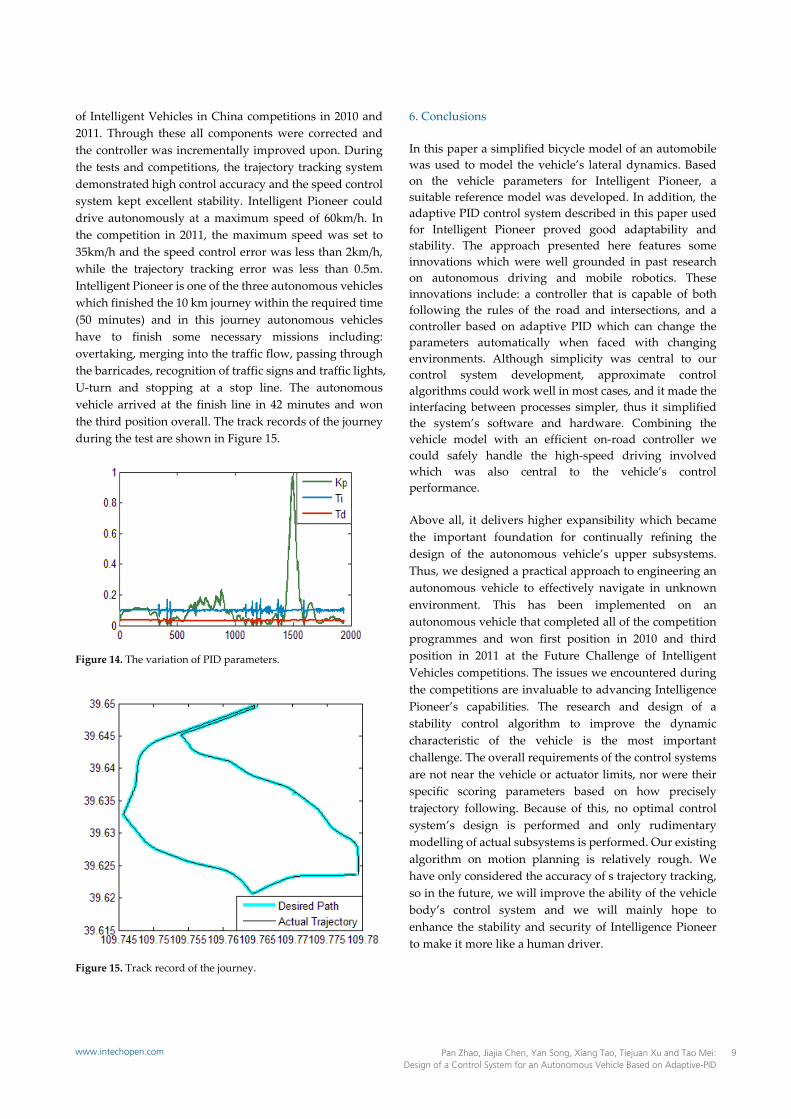
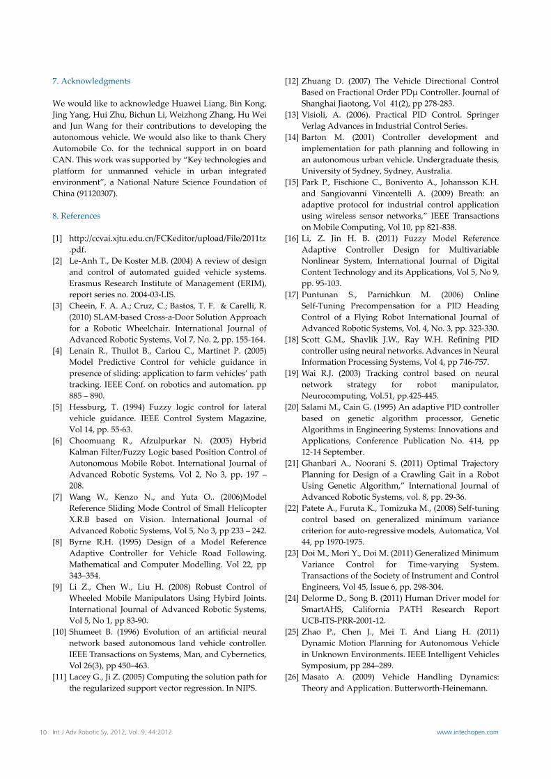
5. Experimental Results and Discussion The performance of this control system is tested on Intelligent Pioneer with different kinds of trajectories. Figure 9 is a screenshot from Google Map, which shows an example of a trajectory that consists of a long. straight part, a long, curved part and a sharp curve. The test is driven at a top speed of approximately 20 m/s. The desired trajectory is reconstructed from the data points with 1m spacing recorded from GPS/INS data (latitude and longitude) and many related data are all recorded in real time at a 30‐Hz update rate. The steering angles are determined by calculating the position errors of the output from the controller which has been experimentally validated. Through the actuation system, the desired steering angle is converted to an absolute encoder position and sent to the steering gear. The performance result of the path followed using the classical PID control algorithm is shown in Figure 10. This illustrates the actual path followed by the vehicle centre mass relative to its desired trajectory reconstructed from real time data. The performance of the control strategy in terms of track error can be seen in Figure 11. It can be seen that the vehicle largely follows the trajectory quite satisfactorily, but the path error becomes larger when turning. The result of path following using the adaptive PID control is shown in Figure 12 and Figure 13. It can be seen that the vehicle follows the trajectory quite satisfactorily both at straight and turning, and in both cases, the errors are kept well within 0.5m less than the PID control (1m) which achieves the desired purpose of this research. In addition, Figure 14 shows the variation of PID parameters. It can be seen that the percentage gain Kp increases with the curvature of the trajectory. Kp is smaller when going straight, ensuring high‐speed stability. Kp is larger when turning, making the dynamic response faster to decrease the lateral error.

START

FINISH

Figure 9. Screenshot from Google Map of the test site.

Figure 10. Trajectory with classical PID control.

Figure 11. Track error of the trajectory above.

Figure 12. Trajectory with adaptive PID control.

Figure 13. Track error of the trajectory above. Our control system has been developed over the course of more than a year and tested in a multitude of scenarios of autonomous operation, as well as at the Future Challenge


of Intelligent Vehicles in China competitions in 2010 and 2011. Through these all components were corrected and the controller was incrementally improved upon. During the tests and competitions, the trajectory tracking system demonstrated high control accuracy and the speed control system kept excellent stability. Intelligent Pioneer could drive autonomously at a maximum speed of 60km/h. In the competition in 2011, the maximum speed was set to 35km/h and the speed control error was less than 2km/h, while the trajectory tracking error was less than 0.5m. Intelligent Pioneer is one of the three autonomous vehicles which finished the 10 km journey within the required time (50 minutes) and in this journey autonomous vehicles have to finish some necessary missions including: overtaking, merging into the traffic flow, passing through the barricades, recognition of traffic signs and traffic lights, U‐turn and stopping at a stop line. The autonomous vehicle arrived at the finish line in 42 minutes and won the third position overall. The track records of the journey during the test are shown in Figure 15.

Figure 14. The variation of PID parameters.

Figure 15. Track record of the journey.

6. Conclusions In this paper a simplified bicycle model of an automobile was used to model the vehicle’s lateral dynamics. Based on the vehicle parameters for Intelligent Pioneer, a suitable reference model was developed. In addition, the adaptive PID control system described in this paper used for Intelligent Pioneer proved good adaptability and stability. The approach presented here features some innovations which were well grounded in past research on autonomous driving and mobile robotics. These innovations include: a controller that is capable of both following the rules of the road and intersections, and a controller based on adaptive PID which can change the parameters automatically when faced with changing environments. Although simplicity was central to our control system development, approximate control algorithms could work well in most cases, and it made the interfacing between processes simpler, thus it simplified the system’s software and hardware. Combining the vehicle model with an efficient on‐road controller we could safely handle the high‐speed driving involved which was also central to the vehicle’s control performance. Above all, it delivers higher expansibility which became the important foundation for continually refining the design of the autonomous vehicle’s upper subsystems. Thus, we designed a practical approach to engineering an autonomous vehicle to effectively navigate in unknown environment. This has been implemented on an autonomous vehicle that completed all of the competition programmes and won first position in 2010 and third position in 2011 at the Future Challenge of Intelligent Vehicles competitions. The issues we encountered during the competitions are invaluable to advancing Intelligence Pioneer’s capabilities. The research and design of a stability control algorithm to improve the dynamic characteristic of the vehicle is the most important challenge. The overall requirements of the control systems are not near the vehicle or actuator limits, nor were their specic scoring parameters based on how precisely trajectory following. Because of this, no optimal control system’s design is performed and only rudimentary modelling of actual subsystems is performed. Our existing algorithm on motion planning is relatively rough. We have only considered the accuracy of s trajectory tracking, so in the future, we will improve the ability of the vehicle body’s control system and we will mainly hope to enhance the stability and security of Intelligence Pioneer to make it more like a human driver.


www.intechopen.com

7. Acknowledgments We would like to acknowledge Huawei Liang, Bin Kong, Jing Yang, Hui Zhu, Bichun Li, Weizhong Zhang, Hu Wei and Jun Wang for their contributions to developing the autonomous vehicle. We would also like to thank Chery Automobile Co. for the technical support in on board CAN. This work was supported by “Key technologies and platform for unmanned vehicle in urban integrated environment”, a National Nature Science Foundation of China (91120307). 8. References [1] http://ccvai.xjtu.edu.cn/FCKeditor/upload/File/2011tz

.pdf. [2] Le‐Anh T., De Koster M.B. (2004) A review of design

and control of automated guided vehicle systems. Erasmus Research Institute of Management (ERIM), report series no. 2004‐03‐LIS.

[3] Cheein, F. A. A.; Cruz, C.; Bastos, T. F. & Carelli, R. (2010) SLAM‐based Cross‐a‐Door Solution Approach for a Robotic Wheelchair. International Journal of Advanced Robotic Systems, Vol 7, No. 2, pp. 155‐164.

[4] Lenain R., Thuilot B., Cariou C., Martinet P. (2005) Model Predictive Control for vehicle guidance in presence of sliding: application to farm vehicles’ path tracking. IEEE Conf. on robotics and automation. pp 885 – 890.

[5] Hessburg, T. (1994) Fuzzy logic control for lateral vehicle guidance. IEEE Control System Magazine, Vol 14, pp. 55‐63.

[6] Choomuang R., Afzulpurkar N. (2005) Hybrid Kalman Filter/Fuzzy Logic based Position Control of Autonomous Mobile Robot. International Journal of Advanced Robotic Systems, Vol 2, No 3, pp. 197 – 208.

[7] Wang W., Kenzo N., and Yuta O.. (2006)Model Reference Sliding Mode Control of Small Helicopter X.R.B based on Vision. International Journal of Advanced Robotic Systems, Vol 5, No 3, pp 233 – 242.

[8] Byrne R.H. (1995) Design of a Model Reference Adaptive Controller for Vehicle Road Following. Mathematical and Computer Modelling. Vol 22, pp 343–354.

[9] Li Z., Chen W., Liu H. (2008) Robust Control of Wheeled Mobile Manipulators Using Hybird Joints. International Journal of Advanced Robotic Systems, Vol 5, No 1, pp 83‐90.

[10] Shumeet B. (1996) Evolution of an artificial neural network based autonomous land vehicle controller. IEEE Transactions on Systems, Man, and Cybernetics, Vol 26(3), pp 450–463.

[11] Lacey G., Ji Z. (2005) Computing the solution path for the regularized support vector regression. In NIPS.

[12] Zhuang D. (2007) The Vehicle Directional Control Based on Fractional Order PDμ Controller. Journal of Shanghai Jiaotong, Vol 41(2), pp 278‐283.

[13] Visioli, A. (2006). Practical PID Control. Springer Verlag Advances in Industrial Control Series.

[14] Barton M. (2001) Controller development and implementation for path planning and following in an autonomous urban vehicle. Undergraduate thesis, University of Sydney, Sydney, Australia.

[15] Park P., Fischione C., Bonivento A., Johansson K.H. and Sangiovanni Vincentelli A. (2009) Breath: an adaptive protocol for industrial control application using wireless sensor networks,” IEEE Transactions on Mobile Computing, Vol 10, pp 821‐838.

[16] Li, Z. Jin H. B. (2011) Fuzzy Model Reference Adaptive Controller Design for Multivariable Nonlinear System, International Journal of Digital Content Technology and its Applications, Vol 5, No 9, pp. 95‐103.

[17] Puntunan S., Parnichkun M. (2006) Online Self‐Tuning Precompensation for a PID Heading Control of a Flying Robot International Journal of Advanced Robotic Systems, Vol. 4, No. 3, pp. 323‐330.

[18] Scott G.M., Shavlik J.W., Ray W.H. Refining PID controller using neural networks. Advances in Neural Information Processing Systems, Vol 4, pp 746‐757.

[19] Wai R.J. (2003) Tracking control based on neural network strategy for robot manipulator, Neurocomputing, Vol.51, pp.425‐445.

[20] Salami M., Cain G. (1995) An adaptive PID controller based on genetic algorithm processor, Genetic Algorithms in Engineering Systems: Innovations and Applications, Conference Publication No. 414, pp 12‐14 September.

[21] Ghanbari A., Noorani S. (2011) Optimal Trajectory Planning for Design of a Crawling Gait in a Robot Using Genetic Algorithm,” International Journal of Advanced Robotic Systems, vol. 8, pp. 29‐36.

[22] Patete A., Furuta K., Tomizuka M., (2008) Self‐tuning control based on generalized minimum variance criterion for auto‐regressive models, Automatica, Vol 44, pp 1970‐1975.

[23] Doi M., Mori Y., Doi M. (2011) Generalized Minimum Variance Control for Time‐varying System. Transactions of the Society of Instrument and Control Engineers, Vol 45, Issue 6, pp. 298‐304.

[24] Delorme D., Song B. (2011) Human Driver model for SmartAHS, California PATH Research Report UCB‐ITS‐PRR‐2001‐12.

[25] Zhao P., Chen J., Mei T. And Liang H. (2011) Dynamic Motion Planning for Autonomous Vehicle in Unknown Environments. IEEE Intelligent Vehicles Symposium, pp 284–289.

[26] Masato A. (2009) Vehicle Handling Dynamics: Theory and Application. Butterworth‐Heinemann.


[27] Campion G., Bastin G., Novel B. (1996) Structural properties and classification of kinematic and dynamic models of wheeled mobile robots, IEEE Trans. Robotics and Automation. Vol 12, pp 47‐62.

[28] Astrom K.J. and Wittenmark B. (1997) Computer Controlled Systems. Prentice‐Hall Information and System Sciences Series, Englewoods Cliffs, N.J., 3 edition.

[29] Prokop R., Husták P., Prokopová Z. (2002) Simple robust controllers: Design, tuning and analysis. International Journal of Control. pp 905‐921,


www.intechopen.com

Documents

Design of a Control System for an Autonomous Vehicle …cdn.intechopen.com/pdfs/38039.pdf · International Journal of Advanced Robotic Systems Design of a Control System for an Autonomous