DESIGN, FABRICATION, INSTALLATION, AND ANALYSIS OF A CLOSED CYCLE DEMONSTRATION

OTEC PLANT

by

Mohammed Faizal

A thesis submitted in fulfillment of the

requirements for the degree of

Master of Science in Engineering

Copyright © 2012 by Mohammed Faizal

School of Engineering and Physics

Faculty of Science, Technology, and Environment

The University of the South Pacific

May 2012

ii

Declaration of Originality Statement by Author

I, Mohammed Faizal, hereby declare that the write up of this dissertation is purely

my own work without the inclusion of any other research materials that has already

been published or written. Any individuals’ work or idea that has been included

within the report has been clearly referenced and credit given to the person.

----------------------

Mohammed Faizal

S11019937

16/05/2012

Statement by Supervisor

I hereby confirm that the work contained in this supervised research project is the

work of Mohammed Faizal unless otherwise stated.

------------------------------

M. Rafiuddin Ahmed (Associate Professor)

Principal Supervisor

16/05/2012

iii

Acknowledgements First of all, I would like to thank the almighty God for giving me the knowledge and

patience to successfully finish this research. I sincerely thank my supervisor,

Associate Professor. M. Rafiuddin Ahmed, for his guidance, assistance and support

in my experiments, publications, and compilation of the thesis.

I am very grateful to the University of the South Pacific, Faculty of Science

and Technology Research Committee for funding this research project. I also owe

gratitude to all the academic and technical staff members of the School of

Engineering and Physics. Special thanks to Mr. Shiu dayal and Mr. Sanjay Singh for

their guidance in technical issues.

To my colleagues Mr. Mohammed Tazil, Mr. Imran Jannif, Mr. Krishnil

Ram, Mr. Sandeep Patel, Mr. Jai Goundar, Mr. Sandeep Reddy, Mr. Shivneel Prasad,

Mr. Jai Goundar, Mr. Ronit Singh, Mr. Epeli Naboloniwaqa, Mr. Binal Raj, Mr.

Vinit Chandra, and Mr. Shahil Ram for helping me with the experiments.

I would like to thank my mother, brother, and sister for their continuous

encouragement throughout the project. I would like to thank all those who have

helped me directly or indirectly to accomplish my Masters Degree, a big milestone in

my life.

iv

Publications

1. Faizal, M, Ahmed MR. On the ocean heat budget and ocean thermal energy

conversion. International Journal of Energy Research 2012; 35: 1119–1144.

doi: 10.1002/er.1885

2. Faizal M, Ahmed MR. Experimental studies on a corrugated plate heat

exchanger for small temperature difference applications, Experimental

Thermal and Fluid Science 2012; 36: 242-248, ISSN 0894-1777,

10.1016/j.expthermflusci.2011.09.019.

3. Faizal M, Ahmed M.R. Experimental studies on a closed cycle

demonstration OTEC plant working on small temperature differences.

Renewable Energy (Under review)

v

Abstract Ocean water covers a vast portion of the earth’s surface and is also the world’s

largest solar energy collector. It plays an important role in maintaining the global

energy balance as well as in preventing the earth’s surface from continually heating

up due to solar radiation. The ocean also plays an important role in driving the

atmospheric processes. The heat exchange processes across the ocean surface are

represented in an ocean thermal energy budget, which is important because the ocean

stores and releases thermal energy. The solar energy absorbed by the ocean heats up

the surface water, despite the loss of heat energy from the surface due to back-

radiation, evaporation, conduction and convection, and the seasonal change in the

surface water temperature is less in the tropics. The cold water from the higher

latitudes is carried by ocean currents along the ocean bottom from the poles towards

the equator, displacing the lower density water above and creating a thermal structure

with a large reservoir of warm water at the ocean surface and a large reservoir of cold

water at the bottom, with a temperature difference of 22ºC to 25ºC between them.

The available thermal energy, which is the almost constant temperature water at the

beginning and end of the thermocline, in some areas of the oceans, is suitable to

drive ocean thermal energy conversion (OTEC) plants. These plants are basically

heat engines that use the temperature difference of the surface and deep ocean water

to drive turbines to generate electricity. An overview of the heat energy budget of the

ocean is presented taking into consideration all the major heat inputs and outputs.

The theoretical analysis of the closed cycle OTEC system is also presented.

Experimental studies were performed on a corrugated plate heat exchanger

for small temperature difference applications. Experiments were performed on a

single corrugation pattern on twenty plates arranged parallelly, with a total heat

transfer area of 1.16298 m2. The spacing, �X, between the plates was varied (�X = 6

mm, 9 mm, and 12 mm) to experimentally determine the configuration that gives the

optimum heat transfer. Water was used on both the hot and the cold channels with

the flow being parallel and entering the heat exchanger from the bottom. The hot

water flowrates were varied. The cold side flowrate and the hot and cold water inlet

temperatures were kept constant. It is found that for a given �X, the average heat

transfer between the two liquids increases with increasing hot water flowrates. The

corrugations on the plates enhance turbulence at higher velocities, which improves

vi

the heat transfer. The optimum heat transfer between the two streams is obtained for

the minimum spacing of �X = 6 mm. The pressure losses are found to increase with

increasing flowrates. The overall heat transfer coefficients, U, the temperature

difference of the two stream at outlet, and the thermal length are also presented for

varying hot water flowrates and �X. The findings from this work would enhance the

current knowledge in plate heat exchangers for small temperature difference

applications and also help in the validation of CFD codes.

A closed cycle demonstration OTEC plant was designed, fabricated, and

installed in the Thermo-fluids Lab, The University of the South Pacific. An

experimental study was carried out on the demonstration plant with the help of

temperature and pressure readings before and after each component. An increase in

the warm water temperature increases the heat transfer between the warm water and

the working fluid, thus increasing the working fluid temperature, pressure, and

enthalpy before the turbine. The performance is better at larger flowrates of the

working fluid and the warm water. It is found that the thermal efficiency and the

power output of the system both increases with increasing operating temperature

difference (difference of warm and cold water inlet temperature). The performance of

the system improves with increasing pressure drop across the turbine. Increasing

turbine inlet temperatures also increase the efficiency and the work done by the

turbine. A maximum efficiency of about 1.5 % was achieved in the system.

vii

Nomenclature A total heat transfer area, m2

AC heat transfer area of condenser, m2

AE heat transfer area of evaporator, m2

b plate spacing, m

Cp specific heat of air (or water) at constant pressure, kJ/kg.ºC

CpCW specific heat at average cold water temperature, kJ/kg.oC

CpHW specific heat at average hot water temperature, kJ/kg.oC

g gravitational acceleration, m/s2

h specific enthalpies, kJ/kg

h,isen isentropic specific enthalpies, kJ/kg

CSm� mass flowrate of cold seawater, kg/s

WFm� mass flowrate of working fluid, kg/s

WSm� mass flowrate of warm seawater, kg/s

N precipitation, cm/year

P operating pressures, Pa

bQ� rate of heat loss from the ocean by back radiation, W/m2

CQ� heat transferred in the OTEC condenser, W

EQ� heat transferred in the OTEC evaporator, W

eQ� rate of heat loss by evaporation from the ocean surface, W/m2

hQ� rate of sensible heat loss from ocean surface by convection and

conduction,W/m2

SQ� rate of heat added to ocean by short-wave solar radiation, W/m2

TQ� total rate of heat gain or loss by a given area of the ocean, W/m2

VQ� heat transport by moving currents (advection) within the ocean, W/m2

CWQ� heat transferred by cold water in the heat exchanger, W

HWQ� heat transferred by hot water in the heat exchanger, W

AverageQ� average heat transfer between hot and cold water in the heat

exchanger, W

S salinity, parts per thousand � ����

viii

Ts ocean surface temperature, ºC

TWSI warm seawater temperature at inlet of evaporator, ºC

TWSO warm seawater temperature at outlet of evaporator, ºC

TCSI cold seawater temperature at inlet of condenser, ºC

TCSO cold seawater at outlet of condenser, ºC

TCWI cold water temperature at inlet of heat exchanger, ºC

TCWO cold water temperature at outlet of heat exchanger, ºC

THWI hot water temperature at inlet of heat exchanger, ºC

THWO hot water temperature at outlet of heat exchanger, ºC

U overall heat transfer coefficient, W/m2.K

UC overall heat transfer coefficient of condenser, W/m2.K

UE overall heat transfer coefficient of evaporator, W/m2.K

CSV� cold seawater flowrate, L/s

CWV� cold water flowrate in corrugated plate heat exchanger, L/s

HWV� hot water flowrate in corrugated plate heat exchanger, L/s

WFV� working fluid flowrate, L/s

WSV� warm seawater flowrate, L/s

V evaporation, cm/year

vf specific volume of liquid working fluid, m3/kg

w amplitude or channel height, m

GW� generator power of OTEC plant, W

NW� net power of OTEC plant, W

CSPW� power required by cold seawater pump, W

WSPW� power required by warm seawater pump, W

WFPW� power required by working fluid pump, W

�PH pressure loss of hot water in the heat exchanger, kPa

�TCW temperature change of cold water in the heat exchanger, ºC

�THW temperature change of hot water in the heat exchanger, ºC

�Tm log mean temperature difference (LMTD) of the heat exchanger, ºC

�Toutlet temperature difference of hot and cold water measured at outlet of

heat exchanger, ºC

ix

�X plate spacing of the heat exchanger, mm

�CW water density at average cold water temperature in heat exchanger,

kg/m3

�HW water density at average hot water temperature in the heat exchanger,

kg/m3

�CW thermal length of the cold water channels of the heat exchanger

�HW thermal length of the hot water channels of the heat exchanger

�Average average thermal length in the heat exchanger �G efficiency of generator

�T efficiency of turbine

�CSP efficiency of cold seawater pump

�WFP efficiency of working fluid pump

�WSP efficiency of warm seawater pump

�hCSP total head loss across cold water piping, m

�hWSP total head loss across warm water piping, m

(�hCS)C head loss in the condenser, m

(�hWS)E head loss in the evaporator, m

(�hCS)d head loss due to density differences in cold water pipe, m

(�hCS)M minor head loss in the cold water pipe, m

(�hWS)M minor head loss in the warm water pipe due to bends, m

(�hCS)SP frictional head loss in straight cold water pipe, m

(�hWS)SP frictional head loss in straight warm water pipe, m

(�Tm)C log mean temperature difference of condenser, ºC

(�Tm)E log mean temperature difference of evaporator, ºC

� seawater density, kg/m3

� wavelength or pitch of corrugated plate, m

� seawater density, kg/m3

x

Table of Contents Declaration of Originality ................................................................................................... ii

Acknowledgements ............................................................................................................iii

Publications ........................................................................................................................ iv

Abstract ............................................................................................................................... v

Nomenclature ....................................................................................................................vii

List of Figures .................................................................................................................... xi

List of Tables ...................................................................................................................xiii

1.0 Introduction................................................................................................................... 1

1.1. Overview................................................................................................................ 1

1.2. Thesis Objectives ................................................................................................... 2

1.3. Thesis Outline ........................................................................................................ 2

2.0 Literature Review.......................................................................................................... 4

2.1. Ocean Thermal Energy Conversion (OTEC)......................................................... 6

2.2. The Thermal Structure of the Ocean.................................................................... 12

2.3 Technological Issues ............................................................................................. 16

2.4. Impacts of OTEC Plants ...................................................................................... 16

2.5. Corrugated Plate Heat Exchangers....................................................................... 18

3.0 Theoretical Analysis of the Closed Cycle OTEC System........................................... 23

4.0 Device Designs, Fabrication, and Experimentation.................................................... 29

4.1. Corrugated Plate Heat Exchanger ........................................................................ 29

4.2. Closed Cycle Demonstration OTEC Plant........................................................... 32

5.0 Experimental Results and Analysis............................................................................. 37

5.1. Corrugated Plate Heat Exchangers....................................................................... 37

5.2. Closed Cycle Demonstration OTEC Plant........................................................... 44

6.0 Conclusions ................................................................................................................. 51

References ......................................................................................................................... 53

Appendix ........................................................................................................................... 64

xi

List of Figures Figure 1.Schematic diagram of heat transfer processes from a given area of the ocean .... 5

Figure 2. Schematic diagram of an OTEC plant operating as a heat engine. .................... 7

Figure 3.Typical mean temperature vs. depth profiles of the open ocean at different

latitudes. ............................................................................................................................ 13

Figure 4. Latitudinal variation of surface temperature, salinity, and density average

for all oceans ..................................................................................................................... 14

Figure 5. Comparison of the amount of radiation received at different latitudes ............ 14

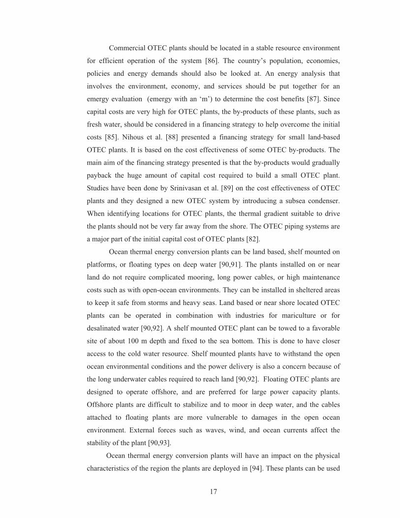
Figure 6 Hot and cold fluid flow in alternate passages in plate heat exchangers. ............ 19

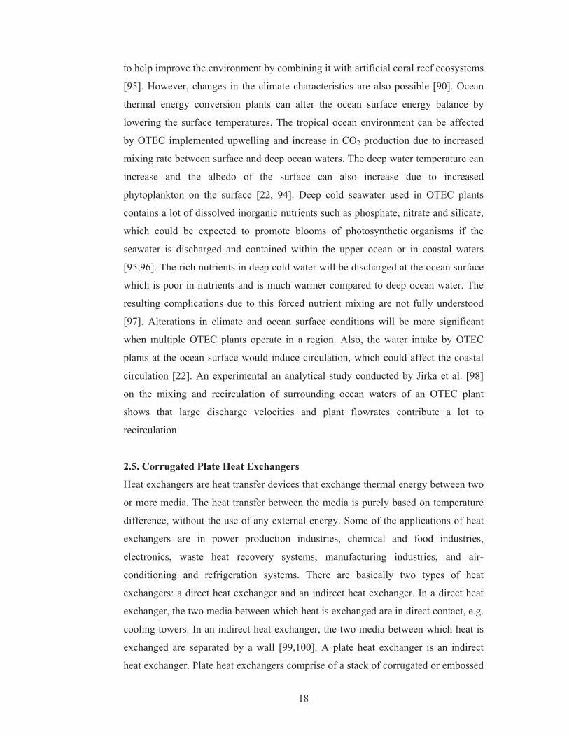
Figure 7. Schematic geometry of corrugated surfaces (� is wavelength or pitch, b is

plate spacing, and w is amplitude or channel height) ....................................................... 20

Figure 8. Schematic diagram of a closed cycle OTEC system and its T-S diagram ....... 23

Figure 9 Geometric details of the heat exchanger plates (dimensions in mm). ................ 30

Figure 10. Schematic diagram of the experimental setup. ................................................ 31

Figure 11. A schematic diagram of the heat exchanger showing exit ports and the

flow dividers used at inlet and exit (blue for cold water and red for hot water). .............. 31

Figure 12. The three fabricated heat exchangers .............................................................. 32

Figure 13. Schematic diagram of the OTEC demonstration plant (P = pressure

gauges, T = Temperature sensors). ................................................................................... 32

Figure 14. The final closed cycle demonstration OTEC plant.......................................... 33

Figure 15. A picture of the spiraled tubes used in the heat exchangers. .......................... 34

Figure 16. A picture of the mini turbine used in the set-up. ............................................ 35

Figure 17. Temperature change of the fluids (difference of inlet and outlet

temperatures of the respective streams) (�X = 12 mm). .................................................. 37

Figure 18. Temperature difference of hot and cold water at the exit of the heat

exchanger against HWV� . .................................................................................................... 38

Figure 19. Average heat transfer between hot and cold water, AverageQ� , at varying HWV� ... 39

Figure 20. Pressure loss of hot water at varying HWV� . ..................................................... 39

Figure 21. The variation of the overall heat transfer coefficient, U, with varying HWV� . .. 40

Figure 22. The variation of the average thermal length, �Average, with varying HWV� ......... 41

Figure 23. The overall heat transfer coefficient, U, presented against the pressure loss

of the hot water, �PH......................................................................................................... 42

xii

Figure 24. Thermal efficiency and power output of the system against operating

temperature difference, for WFV� = 2.5 L/s, and varying WSV� . ............................................ 45

Figure 25. Thermal efficiency and power output of the system against operating

temperature difference, for WFV� = 4.5 L/s, and varying WSV� . ............................................ 45

Figure 26. Turbine inlet pressure and turbine pressure drop against operating

temperature difference, for WSV� = 0.46 L/s and both the WFV� . ......................................... 46

Figure 27. Thermal efficiency and power output of the system against the pressure

drop across the turbine, for WFV� = 2.5 L/s and varying WSV� .............................................. 47

Figure 28. Thermal efficiency and power output of the system against the pressure

drop across the turbine, for WFV� = 4.5 L/s and varying WSV� .............................................. 47

Figure 29. Thermal efficiency and power output of the system against turbine inlet

temperature, for WFV� = 2.5 L/s and varying WSV� . .............................................................. 48

Figure 30. Thermal efficiency and power output of the system against turbine inlet

temperature, for WFV� = 4.5 L/s and varying WSV� . .............................................................. 48

Figure 31. Thermal efficiency and power output of the system against the ratio of the

water flowrates, wsV� / csV� , for WFV� = 2.5 L/s and all warm water temperatures. .............. 49

Figure 32. Thermal efficiency and power output of the system against the ratio of the

water flowrates, wsV� / csV� , for WFV� = 4.5 L/s and all warm water temperatures. .............. 50

xiii

List of Tables Table 1. Geometric details of the heat exchanger plates............................................ 30

1

1.0 Introduction 1.1. Overview

Ocean Thermal Energy Conversion (OTEC) technology utilizes the temperature

difference of warm surface water and deep cold water of the ocean to generate

electricity. An OTEC power plant acts as a ‘heat engine’ that extracts heat energy

from the warm surface water, converts part of that energy to generate electricity

through a turbine, and rejects the remaining heat energy to the cold deep sea water in

a cyclic process. The temperature of the ocean waters generally decreases with

increasing depth, except for polar regions. This region of rapidly changing

temperature is known as the thermocline. It is this region that separates the upper

mixed layer of the ocean with deep ocean water. The thermocline is the deepest in

the tropics and shallowest in the polar regions. Below the thermocline, is a region of

deep cold ocean water where the temperature reaches an almost isothermal condition.

The surface water thus acts as a large reservoir of warm water and the deep water

(approximately at 1000 m) acts as a large reservoir of cold water in the tropical

oceans throughout the year. This uniform temperature difference can be used to

operate OTEC plants.

Ocean Thermal Energy Conversion plants are most suitable in tropical

regions because of less variation in ambient temperature throughout the year around.

Regions closer to the equator have maximum potential for OTEC systems. In

tropical countries, sunlight is abundant in supply and most of the solar energy gets

absorbed by the oceans. This thermal energy available in the oceans can be utilized

to reduce global warming and its consequences. Research in Renewable Energy

technologies creates pathways to reduce the reliance on imported fossil fuels. The

pacific island countries have excellent temperature difference of surface and deep

water (at approximately 1000 m) of the ocean, making this region a better place for

OTEC power generation. The major advantages of OTEC power plants are that they

provide a consistent power output almost throughout the year. Ocean Thermal

Energy Conversion technology is environmental friendly and does not directly

contribute to global warming and depletion of natural resources. It also gives a lot of

useful by-products. A sea-water desalination plant can be integrated into an OTEC

power plant to obtain fresh water. However, it should be noted that this field is still

2

under development and a lot of research still remains to be done to develop power

from OTEC economically.

The current project focused on manufacturing and experimentation of a

closed cycle demonstration OTEC and performing experimental studies on a

corrugated plate heat exchanger. The OTEC plant was designed, fabricated, and

installed in the Thermo-fluids Laboratory, The University of the South Pacific

(USP).

1.2. Thesis Objectives

� To give an overview on the types of OTEC systems, their operational

concepts, the individual components, and overall performance parameters.

� To perform a theoretical analysis of the closed cycle OTEC system.

� To perform experimental studies on corrugated plate heat exchangers for

small temperature difference applications.

� To fabricate and install a closed cycle OTEC demonstration plant in the

Thermo-fluids Lab, USP.

� To experimentally determine the performance of the demonstration OTEC

plant under various operational conditions.

1.3. Thesis Outline

Chapter 1 gives a general introduction of Ocean Thermal Energy Conversion

(OTEC) operating principles. The reasons as to why OTEC plants are suitable for

Pacific Island Countries are also briefly described. The objectives of this research are

also listed.

Chapter 2 gives an overview of the ocean heat budget and the different types

of OTEC plants and its operational principles, the thermal structure of the oceans, the

feasibility and technical limitations of OTEC plants. It also provides a detailed

literature review of corrugated plate heat exchangers.

In chapter 3, a detailed theoretical analysis of the closed cycle OTEC system

is presented.

In chapter 4, the system component designs, fabrication, and experimental

setups are described. The corrugated plate heat exchangers and the final closed cycle

OTEC demonstration plant details are given.

3

Chapter 5 presents the experimental results and analysis of the corrugated

plate heat exchangers and the closed cycle OTEC demonstration plant.

Chapter 6 summarizes the main findings from this research.

4

2.0 Literature Review

The Earth’s surface is approximately covered by seventy percent of water. Ocean

water makes up 97.4% of the total water available [1]. The global-ocean can be

classified as a continuous body of water that separates into several major oceans and

seas [2]. The major ocean divisions, according to their size, are the Pacific Ocean,

Atlantic Ocean, Indian Ocean, Southern Ocean, and the Arctic Ocean [2,3]. The

average temperatures of the ocean waters hardly exceed 30ºC or reduce below -2ºC

[4]. It is the water in the oceans that prevents wide variations of temperature on the

Earth’s surface globally [5].

The amount of heat energy required to raise the temperature of a given mass of

water by 1ºC is more than that of other fluids [6]. Moreover, the ocean has the largest

heat capacity compared to any single component of the climate system [7]. This

property of water allows a lot of solar energy to be stored in the oceans, thus

preventing the Earth’s surface from heating up [5]. The major source of thermal

energy entering the ocean is from the Sun. The ocean plays an important role in

maintaining the global energy balance of the Earth’s atmosphere. The ocean stores

thermal energy to a much greater extent than land because of its high heat capacity

[8]. The ocean can absorb heat in one region and restore it in a different place, even

after decades or centuries [9]. The amount of thermal energy entering the ocean must

be equal to the thermal energy leaving or the average temperature of the ocean will

change [10]. Significant heat exchange processes across the ocean surface are

represented in an ocean energy budget [11]. The ocean energy budget is important

because the ocean stores and releases much more heat than the land over different

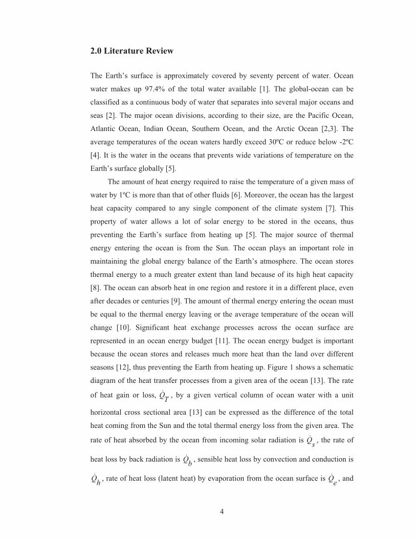
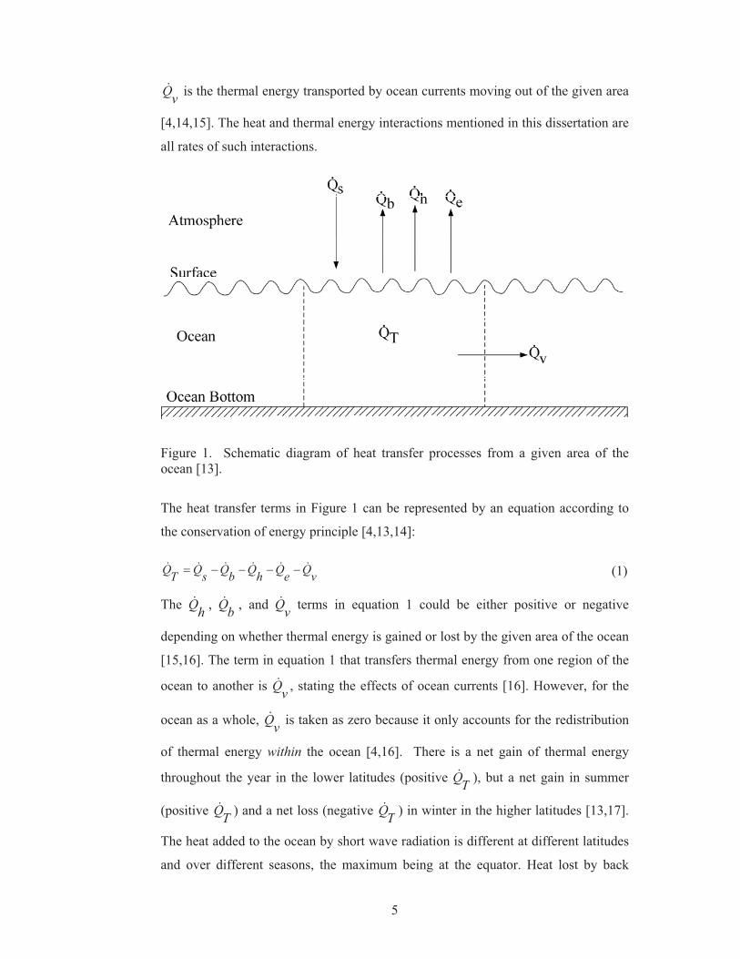
seasons [12], thus preventing the Earth from heating up. Figure 1 shows a schematic

diagram of the heat transfer processes from a given area of the ocean [13]. The rate

of heat gain or loss, TQ� , by a given vertical column of ocean water with a unit

horizontal cross sectional area [13] can be expressed as the difference of the total

heat coming from the Sun and the total thermal energy loss from the given area. The

rate of heat absorbed by the ocean from incoming solar radiation is sQ� , the rate of

heat loss by back radiation is bQ� , sensible heat loss by convection and conduction is

hQ� , rate of heat loss (latent heat) by evaporation from the ocean surface is Qe� , and

5

vQ� is the thermal energy transported by ocean currents moving out of the given area

[4,14,15]. The heat and thermal energy interactions mentioned in this dissertation are

all rates of such interactions.

Figure 1. Schematic diagram of heat transfer processes from a given area of the ocean [13].

The heat transfer terms in Figure 1 can be represented by an equation according to

the conservation of energy principle [4,13,14]:

(1) The hQ� , bQ� , and vQ� terms in equation 1 could be either positive or negative

depending on whether thermal energy is gained or lost by the given area of the ocean

[15,16]. The term in equation 1 that transfers thermal energy from one region of the

ocean to another is vQ� , stating the effects of ocean currents [16]. However, for the

ocean as a whole, vQ� is taken as zero because it only accounts for the redistribution

of thermal energy within the ocean [4,16]. There is a net gain of thermal energy

throughout the year in the lower latitudes (positive TQ� ), but a net gain in summer

(positive TQ� ) and a net loss (negative TQ� ) in winter in the higher latitudes [13,17].

The heat added to the ocean by short wave radiation is different at different latitudes

and over different seasons, the maximum being at the equator. Heat lost by back

vQeQhQbQsQTQ ������ �����

6

radiation from the surface of the ocean increases with decreasing altitudes of the Sun.

The effective back radiation from the ocean surface is the difference of the outward

radiation from the surface and the re-radiation (or down radiation) from the

atmosphere. Heat lost by evaporation from the ocean surface is the largest

contributing factor to the overall heat losses from the ocean. The evaporation is

higher close to the equator and decreases with increasing latitudes. Heat lost by

convection and conduction has seasonal and regional variations, and depends on the

temperature difference of the ocean surface and the air close to the surface. A more

detailed explanation of the heat budget terms are provided by Faizal et al.[18].

The thermal energy in the oceans is distributed around the globe by moving

ocean currents [19]. The circulation of waters in the oceans helps to distribute the

thermal energy in the lower latitudes to certain areas in higher latitudes, thus

modifying climate conditions [20]. The equatorial regions, or the lower latitudes,

receive much more heat from the Sun than the polar regions because of the different

angles at which the sunlight strikes the Earth [5]. The major factors that drive the

ocean currents are solar energy and the Earth’s rotation [21]. Solar energy that is

directly absorbed by the ocean varies from region to region due to unequal heating of

the Earth’s surface [4]. Ocean thermal energy conversion (OTEC) technologies can

be used to extract the thermal energy in oceans.

2.1. Ocean Thermal Energy Conversion (OTEC)

Ocean thermal energy conversion (OTEC) is a technique that utilizes the temperature

difference of warm surface water and deep cold water of the ocean to operate a low

pressure turbine [22,23]. An OTEC power plant acts as a heat engine that extracts

energy as heat from the warm surface water, converts part of that energy to generate

electricity and rejects the remaining energy as heat to the cold deep sea water in a

cyclic process [22,24]. It can be integrated with a desalination plant, commonly

known as the hybrid cycle, to produce fresh water [25,26]. Ocean Thermal Energy

Conversion plants are more suitable for low latitudes (tropical oceans) because the

water temperature remains almost uniform throughout the year with few variations

due to seasonal effects [23]. About 63% of the surface of the tropics between

latitudes 30ºN and 30ºS is occupied by ocean water [27].

Solar energy that is absorbed by the tropical oceans maintains a relatively

stable surface temperature of 26-28ºC to a depth of approximately 100 m. As the

7

depth increases, the temperature drops, and at depths close to 1000 m, the

temperature is as low as 4ºC. Below this depth, the temperature drops only a few

degrees. The temperature difference of warm and cold waters is maintained

throughout the year with very few variations in the tropics. From the view of a

thermodynamicist, any temperature difference can be used to generate power [22].

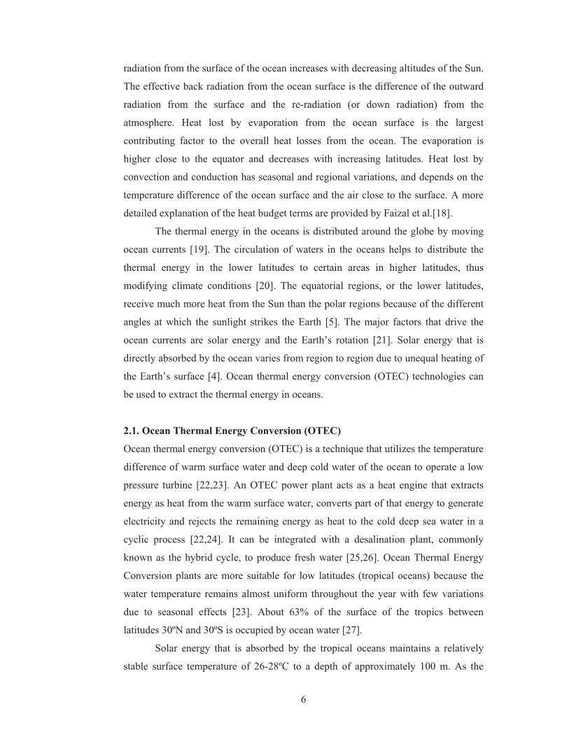
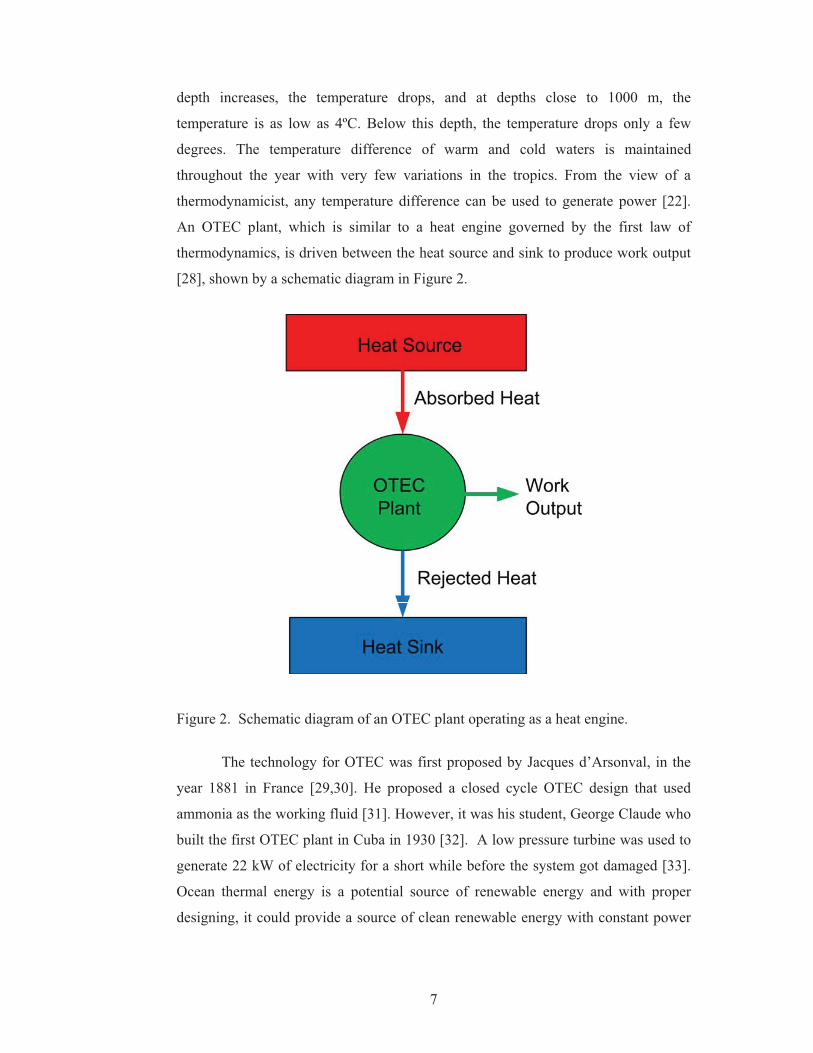
An OTEC plant, which is similar to a heat engine governed by the first law of

thermodynamics, is driven between the heat source and sink to produce work output

[28], shown by a schematic diagram in Figure 2.

Figure 2. Schematic diagram of an OTEC plant operating as a heat engine.

The technology for OTEC was first proposed by Jacques d’Arsonval, in the

year 1881 in France [29,30]. He proposed a closed cycle OTEC design that used

ammonia as the working fluid [31]. However, it was his student, George Claude who

built the first OTEC plant in Cuba in 1930 [32]. A low pressure turbine was used to

generate 22 kW of electricity for a short while before the system got damaged [33].

Ocean thermal energy is a potential source of renewable energy and with proper

designing, it could provide a source of clean renewable energy with constant power

8

output with many other benefits such as pure drinking water, which can benefit many

small islands and developing countries [34].

Ocean thermal energy conversion power systems are basically divided into

three categories: open cycle, closed cycle, and hybrid systems. An open cycle OTEC

system utilizes the warm surface water as the working fluid. The surface water is

pumped into a chamber where a vacuum pump reduces the pressure to allow the

water to boil at low temperature to produce steam. The steam drives a turbine

coupled to a generator and then is condensed (using deep cold seawater pumped to

the surface) to produce desalinated water [22,35]. A closed cycle OTEC system

incorporates a working fluid, such as ammonia or ammonia/water mixture, operating

between two heat exchangers in a closed cycle. A closed cycle utilizes the warm

surface water to vaporize the working fluid in a heat exchanger (evaporator). The

vaporized fluid drives a turbine coupled to a generator. The vapor is then condensed

in a heat exchanger (condenser) using cold deep seawater pumped to the surface. The

condensed working fluid is pumped back to the evaporator and the cycle is repeated.

Major differences between the open and closed cycle systems are the sizes of ducts

and turbines, and the surface area required by heat exchangers for effective heat

transfer [22]. For a given OTEC system with a certain power output, a closed cycle

system with ammonia as the working fluid requires a much smaller duct and turbine

diameter compared to an open cycle system which has water as the working fluid

[36]. The difference is attributed to the pressure difference across the turbine and the

specific volume of the working fluids. The heat exchangers for closed cycle systems

require large surface areas to minimize temperature losses and to maintain the heat

transfer between the ocean water and the working fluid to obtain the required power

output [22].

The hybrid system integrates the power cycle with desalination to produce

electricity and desalinated water. Nearly 2.28 million liters of desalinated water can

be obtained everyday for every MW of power generated by a hybrid OTEC system

[37]. Electricity is generated in the closed cycle system circulating a working fluid

and the warm and cold seawater discharges are passed through a vacuum chamber

and condenser to produce fresh water [22]. The power that the pumps need to do

work is supplied from the gross power output of the OTEC power generating system.

The working fluids for either closed or hybrid cycles should be such that it is able to

operate between the low temperatures and still give optimum efficiency. Mostly

9

Freon and ammonia are considered, whereas ammonia and water mixture are also

accepted for use [38]. The use of mixtures instead of one component fluid improves

the thermodynamic performance of power cycles [39]. Studies done by Kim et al.

[40] suggests that working fluids can be selected based on the specific environment

and working conditions without affecting the efficiency much. The OTEC cycles are

basic Rankine cycles that operate between a heat source and sink to generate

electricity [41,42] with efficiencies close to 3% [41]. To increase the thermal

efficiency of the OTEC system, other kinds of energies such as solar energy,

geothermal energy, industrial waste energy, and solar ponds can be introduced to

increase the temperature difference [43-45].

A lot of research work has been carried out on OTEC since its discovery in

1881. The first ever OTEC plant that was successfully commissioned was in Hawaii

in 1979. A 50 kW closed cycle floating demonstration plant was constructed

offshore. Cold water at a temperature of 4.4 °C was drawn from a depth of 670 m.

During actual operation of the plant, it was found that biofouling, effects of mixing

the deep cold water with the warm surface water, and debris clogging did not have

any negative effects on plant operation. The longest continuous operation was for

120 hours [46]. A 100 kW OTEC pilot plant was constructed on-land for

demonstration purposes in the republic of Nauru in October 1981 by Japan. The

system operated between the warm surface water and the cold heat source of 5-8°C

at a depth of 500-700 m, with a temperature difference of 20°C [47]. The tests done

were load response characteristics, turbine, and heat exchanger performance tests.

The plant had operated by two shifts withy one spare shift, and a continuous power

generation record of ten days was achieved. The plant produced 31.5 kW of OTEC

net power during continuous operation and was connected to the main power grid

[47].

A land based open cycle OTEC experimental plant was installed in Hawaii in

1993. The turbine-generator was designed for an output of 210 kW for 26 °C warm

surface water and 6 °C deep water temperature. The highest gross power achieved

was 255 kWe with a corresponding net power of 103 kW and 0.4 L/s of desalinated

water [25]. Saga University, Japan, is actively involved in OTEC and its byproduct

studies. Experimental studies have been conducted on heat exchangers and on spray-

flash evaporation desalination. Other studies done are on mineral water production

using deep cold water, lithium extraction from seawater, hydrogen production, air-

10

conditioning and aquaculture applications using deep cold water, and using the deep

cold water for food processing and medical (cosmetic) applications [48].

Uehara et. al [42] presented a conceptual design for an OTEC plant in the

Philippines after taking extensive temperature readings to determine a suitable site.

The ocean surface water had a temperature range of 25 to 29ºC throughout the year

while the cold water remained between 4 to 8 ºC at a depth of 500 – 700 m. A total

of 14 sites were suggested. A conceptual design for a 5 MW onland-type and a 25

MW floating-type were computed for. After doing cost estimates of the proposed

systems, the construction of the 5 MW onland-type plant was suggested.

Uehara and Ikegami [49] performed an optimization study of a closed cycle

OTEC system. They presented numerical results for a 100 MW OTEC plant with

plate heat exchangers and ammonia as the working fluid. They concluded that the net

power can reach upto 70.3% of the gross power of 100 MW for inlet warm water

temperature of 26 ºC and inlet cold water temperature of 4 ºC. Yeh et al. [50]

conducted a theoretical investigation on the effects of the temperature and flowrate

of cold sea water on the net output of an OTEC plant. They found out that the

maximum net output exists at a certain flowrate of the cold seawater. The output is

higher for a larger ratio of warm to cold seawater flowrate. Uehara et al. [51] did a

performance analysis of an integrated hybrid OTEC plant. The plant is a combination

of a closed cycle OTEC plant and a spray flash desalination plant. The total heat

transfer area of the heat exchangers per net power is used as an objective function. A

numerical analysis was done for a 10 MW integrated hybrid plant. Straatman and

Sark [45] proposed a new hybrid OTEC with an offshore solar pond to optimize

costs of electricity. This proposed system would increase the OTEC efficiency from

3% to 12%. The addition of a floating offshore solar pond to an OTEC system

increases the temperature difference in the power cycle.

Yamada et al. [52] did a performance simulation of a solar-boosted ocean

thermal energy conversion plant, termed as SOTEC. The temperature of warm sea

water used in the evaporator was increased by using a solar thermal collector. The

simulation results showed that the proposed SOTEC plant can increase the overall

efficiency of the OTEC system. Tong et al. [44] proposed a solar energy reheated

power cycle to improve performance. They suggested that a solar collector

introduced at the evaporator will greatly improve the temperature difference and thus

the cycle performance. Also, it was found that without any additional loadings on the

11

heat exchangers, increasing the turbine inlet pressure will also improve the OTEC

system performance. Ganic and Wu [53] analyzed the effect of three working fluids

used in OTEC systems. The fluids studied were ammonia, propane, and Freon-114.

Seven different combinations of shell-and-tube heat exchangers were considered and

for each combination, a computer model of the OTEC system was used. The

comparisons were made based on the total heat transfer area of the heat exchangers

divided by the net power output of the plant. It was found that ammonia was the best

fluid because of its relatively high thermal conductivity. Kim et al. [54] did a

numerical analysis for the same conditions but with various working fluids for a

closed system, a regeneration system, an open system, a Kalina system, and a hybrid

system. They concluded that the regeneration system using R125 as the working

fluid had better performance. They also found that using the condenser effluent of a

nuclear power plant rather than ocean surface water increased the system efficiency

by approximately 2%.

Moore and Martin [55] presented a general mathematical framework for the

synthesis of OTEC power generating systems. They developed a systematic

methodology which was demonstrated in an OTEC system with ammonia as the

working fluid. The power generated was used to drive a PEM electrolyser for

hydrogen production. Faizal and Ahmed [56] performed experimental studies on

corrugated plate heat exchangers for small temperature applications. They varied the

channel spacing. They found that the minimum channel spacing gave optimal heat

transfer. However, there was no phase change involved in their experiments. Zhou et

al. [57] have presented a techno-economic study on compact heat exchangers to

choose an optimum heat exchanger with minimum pressure drop. They concluded

that all compact heat exchangers are feasible from an energetic point of view.

However, the performance differs because of the materials used. Experimental

studies on heat exchangers for use in OTEC plants have also been conducted in Saga

University, Japan [22]. Together with an appropriate pressure difference across the

turbine, a high heat transfer rate between the working fluid and the ocean water in

the heat exchangers is required for optimal power production in OTEC plants [22].

Even though the thermal resource is available to many countries, there are

many factors that have to be considered before a particular country or location is

selected for an OTEC plant installation. Some of them are: distance of the thermal

resource from land; depth of the ocean bed; depth of the resource; size of the thermal

12

resource within the exclusive economic zone (EEZ); replenishment capability for

both warm and cold water; ocean currents; waves; hurricanes; seabed conditions for

mounting; seabed conditions for power cables of floating plants; current local power

source; annual consumption; present cost per unit; local oil or coal production; scope

for other renewables; aquaculture potential; potable water potential; and

environmental impacts [58]. Apart from generating electricity and producing fresh

water, OTEC plants can be utilized for other benefits such as production of fuels

such as hydrogen, ammonia, methanol, providing air-conditioning for buildings, on-

shore and near-shore mariculture, and extraction of minerals [28,59,60]. Pacific

Island countries have a lot of potential for implementation of OTEC technologies

because of the high ocean temperature gradient.

2.2. The Thermal Structure of the Ocean

The temperature of the ocean waters generally decreases with increasing depth,

except for polar regions [6,61]. The surface layer of the oceans is usually referred to

as the mixed layer, because the near-surface waters are well mixed by winds and

waves and a nearly isothermal condition is maintained [4,22]. Below the mixed layer

is a region of rapidly changing temperature known as the thermocline. It is this

region that separates the upper mixed layer of the ocean with deep ocean water [62].

The characteristics of the thermocline vary with season, latitudes, environmental

conditions and ocean currents. The thermocline is the deepest in the tropics and

shallower in the polar regions [63]. Below the thermocline is a region of deep cold

ocean water where the temperature reaches an almost isothermal condition [64]. The

deep cold ocean water is transferred from the polar latitudes [21,22]. The surface

water thus acts as a large reservoir of warm water and the deep water (approximately

at 1000 m) acts as a large reservoir of cold water in the tropical oceans throughout

the year [22]. This uniform temperature difference can be used to operate OTEC

plants [65].

Below the ocean surface water, the water is usually divided into three zones

based on the temperature structure of the ocean: an upper zone with a depth of

approximately 50 to 200 m with temperatures similar to that of the surface, a zone

below 200 m and extending upto 1000 m in which the temperature changes rapidly

(this is the thermocline), and a zone below 1000 m in which the temperature changes

are small [66]. The actual depth of the zones is difficult to determine because of the

13

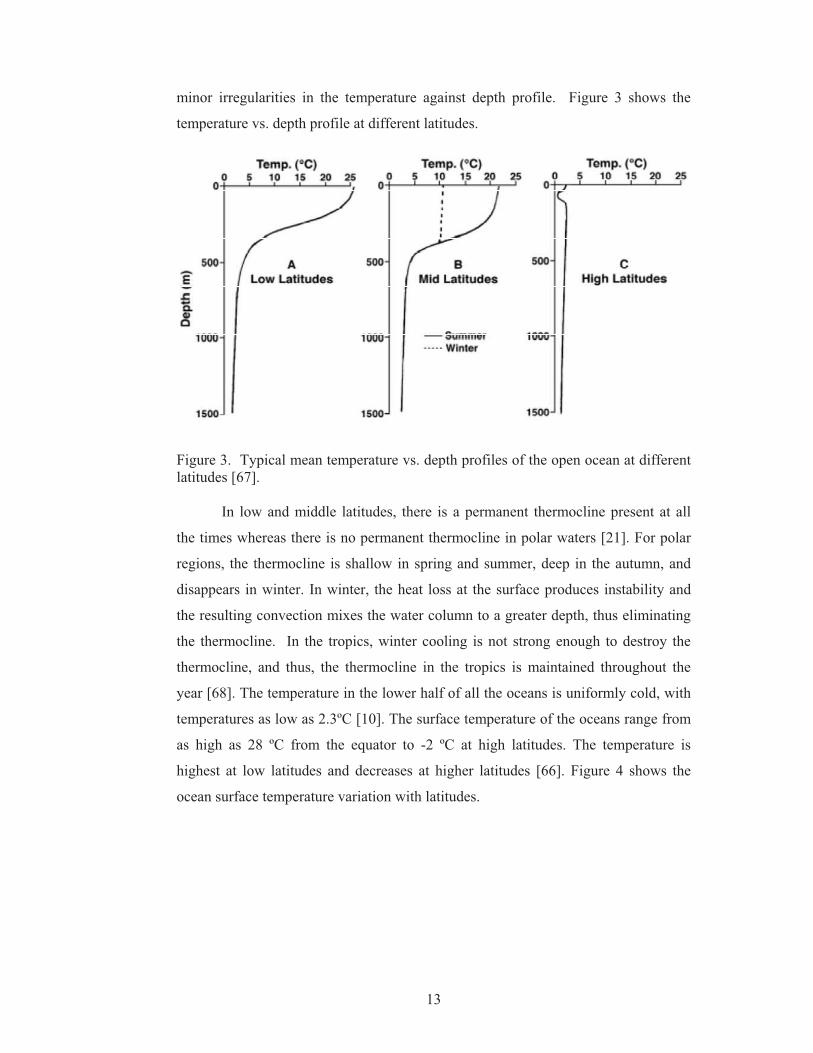
minor irregularities in the temperature against depth profile. Figure 3 shows the

temperature vs. depth profile at different latitudes.

Figure 3. Typical mean temperature vs. depth profiles of the open ocean at different latitudes [67].

In low and middle latitudes, there is a permanent thermocline present at all

the times whereas there is no permanent thermocline in polar waters [21]. For polar

regions, the thermocline is shallow in spring and summer, deep in the autumn, and

disappears in winter. In winter, the heat loss at the surface produces instability and

the resulting convection mixes the water column to a greater depth, thus eliminating

the thermocline. In the tropics, winter cooling is not strong enough to destroy the

thermocline, and thus, the thermocline in the tropics is maintained throughout the

year [68]. The temperature in the lower half of all the oceans is uniformly cold, with

temperatures as low as 2.3ºC [10]. The surface temperature of the oceans range from

as high as 28 ºC from the equator to -2 ºC at high latitudes. The temperature is

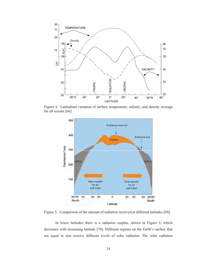
highest at low latitudes and decreases at higher latitudes [66]. Figure 4 shows the

ocean surface temperature variation with latitudes.

14

Density

Figure 4. Latitudinal variation of surface temperature, salinity, and density average for all oceans [66].

Figure 5. Comparison of the amount of radiation received at different latitudes [69].

In lower latitudes there is a radiation surplus, shown in Figure 5, which

decreases with increasing latitude [70]. Different regions on the Earth’s surface that

are equal in size receive different levels of solar radiation. The solar radiation

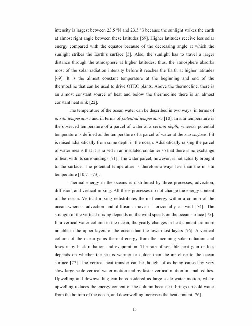
15

intensity is largest between 23.5 ºN and 23.5 ºS because the sunlight strikes the earth

at almost right angle between these latitudes [69]. Higher latitudes receive less solar

energy compared with the equator because of the decreasing angle at which the

sunlight strikes the Earth’s surface [5]. Also, the sunlight has to travel a larger

distance through the atmosphere at higher latitudes; thus, the atmosphere absorbs

most of the solar radiation intensity before it reaches the Earth at higher latitudes

[69]. It is the almost constant temperature at the beginning and end of the

thermocline that can be used to drive OTEC plants. Above the thermocline, there is

an almost constant source of heat and below the thermocline there is an almost

constant heat sink [22].

The temperature of the ocean water can be described in two ways: in terms of

in situ temperature and in terms of potential temperature [10]. In situ temperature is

the observed temperature of a parcel of water at a certain depth, whereas potential

temperature is defined as the temperature of a parcel of water at the sea surface if it

is raised adiabatically from some depth in the ocean. Adiabatically raising the parcel

of water means that it is raised in an insulated container so that there is no exchange

of heat with its surroundings [71]. The water parcel, however, is not actually brought

to the surface. The potential temperature is therefore always less than the in situ

temperature [10,71–73].

Thermal energy in the oceans is distributed by three processes, advection,

diffusion, and vertical mixing. All these processes do not change the energy content

of the ocean. Vertical mixing redistributes thermal energy within a column of the

ocean whereas advection and diffusion move it horizontally as well [74]. The

strength of the vertical mixing depends on the wind speeds on the ocean surface [75].

In a vertical water column in the ocean, the yearly changes in heat content are more

notable in the upper layers of the ocean than the lowermost layers [76]. A vertical

column of the ocean gains thermal energy from the incoming solar radiation and

loses it by back radiation and evaporation. The rate of sensible heat gain or loss

depends on whether the sea is warmer or colder than the air close to the ocean

surface [77]. The vertical heat transfer can be thought of as being caused by very

slow large-scale vertical water motion and by faster vertical motion in small eddies.

Upwelling and downwelling can be considered as large-scale water motion, where

upwelling reduces the energy content of the column because it brings up cold water

from the bottom of the ocean, and downwelling increases the heat content [76].

16

2.3 Technological Issues

The proper designs of OTEC systems include the consideration of leakage of piping

systems that carry the working fluid in a closed cycle. A major disadvantage of

OTEC systems is the high capital cost [29,77]. Extensive research has been done on

the OTEC components, for example, heat exchangers should have compact designs

with optimum heat transfer and low unit cost [78]. Experimental studies on heat

exchangers for use in OTEC plants have also been conducted in Saga University,

Japan [22]. Biofouling in the heat exchangers provides resistance to heat transfer,

therefore affecting their performance [79]. Cleaning methods such as continual

circulation of close fitting balls and by chemical additives to the water are used [79].

Another major design concern is the cold water pipes that transport cold

water from the ocean depths to the surface. The cold water pipes that pump deep cold

ocean water to the surface require a lot of pumping power which increases the costs

[50]. Approximately 4 m3/s of warm surface seawater and 2 m3/s of deep cold

seawater (ratio 2:1), for a temperature difference of 20 ºC, are required for every

MW of electricity generated [80]. The cold water pipes are subjected to forces such

as drag by ocean currents, oscillation forces, stresses at the connections, forces due to

harmonic motion of the platform, and the dead weight of the pipe itself. Also,

problems will arise in installation due to difficulties in construction and

transportation to deployment site due to its very large size. The choice of materials is

also debatable [22,79, 81]. The successful installations of offshore oil drilling

platforms have provided technical guidance that can be directly applicable to OTEC

cold water pipe design [22].

2.4. Impacts of OTEC Plants

Ocean thermal energy conversion plants can be located across about 60 million

square kilometers of tropical oceans, generally at latitudes within about 20 or 25

degrees of the equator. The vast resource of cold water is constantly supplied by the

deep cold water that flows from the polar regions [22,82].

The ocean thermal gradient essential for OTEC plants operation is mostly

found between latitudes 20ºN and 20ºS [83,84]. There are at least two separate

markets for OTEC plants: (i) industrial nations and islands, (ii) smaller or less

industrialized islands with modest needs for power as well as desalinated water [85].

17

Commercial OTEC plants should be located in a stable resource environment

for efficient operation of the system [86]. The country’s population, economies,

policies and energy demands should also be looked at. An energy analysis that

involves the environment, economy, and services should be put together for an

emergy evaluation (emergy with an ‘m’) to determine the cost benefits [87]. Since

capital costs are very high for OTEC plants, the by-products of these plants, such as

fresh water, should be considered in a financing strategy to help overcome the initial

costs [85]. Nihous et al. [88] presented a financing strategy for small land-based

OTEC plants. It is based on the cost effectiveness of some OTEC by-products. The

main aim of the financing strategy presented is that the by-products would gradually

payback the huge amount of capital cost required to build a small OTEC plant.

Studies have been done by Srinivasan et al. [89] on the cost effectiveness of OTEC

plants and they designed a new OTEC system by introducing a subsea condenser.

When identifying locations for OTEC plants, the thermal gradient suitable to drive

the plants should not be very far away from the shore. The OTEC piping systems are

a major part of the initial capital cost of OTEC plants [82].

Ocean thermal energy conversion plants can be land based, shelf mounted on

platforms, or floating types on deep water [90,91]. The plants installed on or near

land do not require complicated mooring, long power cables, or high maintenance

costs such as with open-ocean environments. They can be installed in sheltered areas

to keep it safe from storms and heavy seas. Land based or near shore located OTEC

plants can be operated in combination with industries for mariculture or for

desalinated water [90,92]. A shelf mounted OTEC plant can be towed to a favorable

site of about 100 m depth and fixed to the sea bottom. This is done to have closer

access to the cold water resource. Shelf mounted plants have to withstand the open

ocean environmental conditions and the power delivery is also a concern because of

the long underwater cables required to reach land [90,92]. Floating OTEC plants are

designed to operate offshore, and are preferred for large power capacity plants.

Offshore plants are difficult to stabilize and to moor in deep water, and the cables

attached to floating plants are more vulnerable to damages in the open ocean

environment. External forces such as waves, wind, and ocean currents affect the

stability of the plant [90,93].

Ocean thermal energy conversion plants will have an impact on the physical

characteristics of the region the plants are deployed in [94]. These plants can be used

18

to help improve the environment by combining it with artificial coral reef ecosystems

[95]. However, changes in the climate characteristics are also possible [90]. Ocean

thermal energy conversion plants can alter the ocean surface energy balance by

lowering the surface temperatures. The tropical ocean environment can be affected

by OTEC implemented upwelling and increase in CO2 production due to increased

mixing rate between surface and deep ocean waters. The deep water temperature can

increase and the albedo of the surface can also increase due to increased

phytoplankton on the surface [22, 94]. Deep cold seawater used in OTEC plants

contains a lot of dissolved inorganic nutrients such as phosphate, nitrate and silicate,

which could be expected to promote blooms of photosynthetic organisms if the

seawater is discharged and contained within the upper ocean or in coastal waters

[95,96]. The rich nutrients in deep cold water will be discharged at the ocean surface

which is poor in nutrients and is much warmer compared to deep ocean water. The

resulting complications due to this forced nutrient mixing are not fully understood

[97]. Alterations in climate and ocean surface conditions will be more significant

when multiple OTEC plants operate in a region. Also, the water intake by OTEC

plants at the ocean surface would induce circulation, which could affect the coastal

circulation [22]. An experimental an analytical study conducted by Jirka et al. [98]

on the mixing and recirculation of surrounding ocean waters of an OTEC plant

shows that large discharge velocities and plant flowrates contribute a lot to

recirculation.

2.5. Corrugated Plate Heat Exchangers

Heat exchangers are heat transfer devices that exchange thermal energy between two

or more media. The heat transfer between the media is purely based on temperature

difference, without the use of any external energy. Some of the applications of heat

exchangers are in power production industries, chemical and food industries,

electronics, waste heat recovery systems, manufacturing industries, and air-

conditioning and refrigeration systems. There are basically two types of heat

exchangers: a direct heat exchanger and an indirect heat exchanger. In a direct heat

exchanger, the two media between which heat is exchanged are in direct contact, e.g.

cooling towers. In an indirect heat exchanger, the two media between which heat is

exchanged are separated by a wall [99,100]. A plate heat exchanger is an indirect

heat exchanger. Plate heat exchangers comprise of a stack of corrugated or embossed

19

metal plates with inlet and outlet ports and seals to direct the flow in alternate

channels. The flow channels are formed by adjacent plates [101]. As shown in Figure

6, the hot and cold fluids flow in alternate channels and the heat transfer takes place

between adjacent channels [102]. The number and size of the plates are determined

by the flowrates, the physical properties of the fluids, pressure drops, and heat

transfer requirements [101,103]. There are also many flow patterns that can be

achieved for plate heat exchangers [101].

Figure 6. Hot and cold fluid flow in alternate passages in plate heat exchangers.

In the analysis of heat exchangers, all the thermal resistances in the path of

heat flow from one fluid to another are combined into a single resistance [104], and

an overall heat transfer coefficient, U, of the heat exchanger is determined. The

overall heat transfer coefficient is a measure of the resistance to heat flow from one

medium to another [100]. Phase change processes in heat exchangers have very high

U values due to high thermal conductivities. Because of complex physical processes,

it is not generally possible to predict accurate values of U. Therefore, empirical

formulas and U values are mostly derived from experimental data [105]. One of the

requirements in ocean thermal energy conversion (OTEC) plants is effective heat

transfer with minimum pressure loss for small temperature difference of the hot and

cold fluids. Pressure losses in heat exchangers will affect the pumping power of the

pumps in OTEC plants. Studies reported by Bellas et al. [106] and Uehara et al. [107

show that pressure drop increases significantly with flowrates.

Plate heat exchangers have many advantages compared to many other heat

exchangers. Plate heat exchangers can be used for high-viscosity applications,

because turbulence is induced at low velocities which leads to effective heat transfer

20

[101]. They also have high thermal effectiveness, large heat transfer per unit volume,

low weight, possibility of heat transfer between many streams, ease of maintenance

and a compact design [103, 108].

Corrugations in plate heat exchangers improve the heat transfer rates by 20%

- 30% by increasing the heat transfer area and by enhancing turbulence at low

flowrates [105, 109]. The corrugated plates also improve the mechanical strength of

the plates [102]. Many types of enhanced surface geometries are used on plate heat

exchangers. The objective is to obtain high heat-transfer coefficients without

correspondingly increased pressure-loss penalties [110]. Special channel shapes,

such as the wavy channels, provide mixing due to secondary flows or boundary layer

separation within the channel [101]. The corrugations or wavy fins induce secondary

flows (Görtler vortices) which assist in heat transfer augmentation [111]. The

performance of plate heat exchangers can be improved by modifying the boundary

layer and by enlarging the surfaces [112].

Since wavy surfaces have noninterrupted walls in each flow channel, the

chances of fouling and particulates being caught in the channels are less. The

waveform in the flow direction disrupts the flow and induces very complex flows.

Görtler vortices are formed as the fluid passes over the concave wavy surfaces which

enhance heat transfer. In the low-turbulence regime (Re of about 6000 to 8000), the

wall corrugations increase the heat transfer by about nearly three times compared

with the smooth wall channel [101]. Therefore, wavy fins are often a better choice at

higher Reynolds numbers. A basic form of a corrugated or wavy geometry is shown

in Figure 7. As corrugation (or wave) height to wavelength ratio increases, the

separation zones in the troughs increase in relative size, giving rise to

disproportionately high pressure drop [111]. A variety of corrugated or wavy patterns

are proposed for plate heat exchangers [101].

Figure 7. Schematic geometry of corrugated surfaces (� is wavelength or pitch, b is plate spacing, and w is amplitude or channel height) [113].

21

Several studies have been carried out on heat transfer enhancement using

corrugated plate heat exchangers. Picon-Nuñez et al. [103] presented a methodology

on the design of compact heat exchangers. A simple approach to surface selection of

the heat exchangers is based on the volume performance index. Plain-fin (wavy

configuration) and louvered fins were considered in their study. They presented the

volume performance index at different Reynolds numbers.. Taucher and Mayinger

[112] carried out numerical and experimental studies on heat transfer enhancement in

plate heat exchangers with rib-roughened surfaces, which are also wavy

configurations. They tested for various configurations of the ribs: shape, width,

height, groove angle, spacing, angle, and arrangement patterns. They found out that

the ribs show their best effects in regions where they can induce turbulence. They

generalized that turbulence promoters (ribs in this case) show best performance in

the transition region from laminar to turbulent flow.

Ciofalo et al. [113] conducted studies of flow and heat transfer in corrugated

– undulated plate heat exchanges for rotary regenerators. For a particular corrugation,

they varied the angle between the main flow direction and the axes of the furrows of

the corrugations. They presented the Nusselt number distributions, the friction

coefficient, pressure drop and heat transfer characteristics, and numerically simulated

results on the flow and thermal fields induced by the wavy configurations. Kanaris et

al. [114] performed CFD studies on a plate heat exchanger comprising of corrugated

walls with herringbone design. They visualized the complex swirling flow in the

furrows of the corrugations, and the Nusselt number and the friction factor were

compared with those of smooth plates. They reported that corrugations increase the

heat transfer; however, the pressure losses also increase. Elshafei et al. [115]

presented heat transfer and pressure drop results in corrugated channels. They

discussed the effect of channel spacing and phase shift of the corrugations on the

heat transfer and the pressure drop. They showed that corrugations enhance heat

transfer but with accompanying pressure drops. The results from the experiments

were compared with conventional parallel plate heat exchangers and they found that

corrugations enhance the heat transfer significantly. They found that the friction

factor is higher for higher values of channel spacing. They also concluded that the

area goodness factor decreases with increasing spacing ratio. Sparrow et al. [116]

also performed experimental studies on corrugated plates and variable spacings.

22

Stasiek et al. [117] investigated the flow and heat transfer in corrugated

passages. An experimental and numerical study of flow and heat transfer was

conducted for a crossed-corrugated geometry. The effects of corrugation angle,

geometry, and Reynolds number were investigated. Mitsumori et al. [118, 119]

compared the performance of a closed cycle ocean thermal energy conversion

(OTEC) plant using plate-type heat exchangers and tube-type heat exchangers. The

results of their studies show that plate-type heat exchangers have more advantages

and that they can be more compact. Test results on plate heat exchangers done at

Saga University, Japan are presented by Avery and Wu [105]. It was found that the

overall heat transfer coefficients and the pressure losses generally increase as the

water velocity is increased. The best configurations tested at Saga University

increase the overall heat transfer by a factor of 4 in comparison with smooth plates.

Lyytikäinen et al. [120] performed numerical studies for varying corrugation angles

and corrugation lengths and found out that both heat transfer as well as pressure drop

increase as the corrugation angle is increased. They stated that it is not easy to find a

specific geometry that provides both a low pressure drop and a high heat transfer

simultaneously.

From the previous research carried out on heat transfer enhancement, it is

obvious that wavy corrugations for plate heat exchangers are an attractive option. On

the basis of the above finding, the present work is aimed at experimentally studying

the heat transfer characteristics (with pressure drops) for corrugated plate type heat

exchangers for use in small temperature difference applications.

23

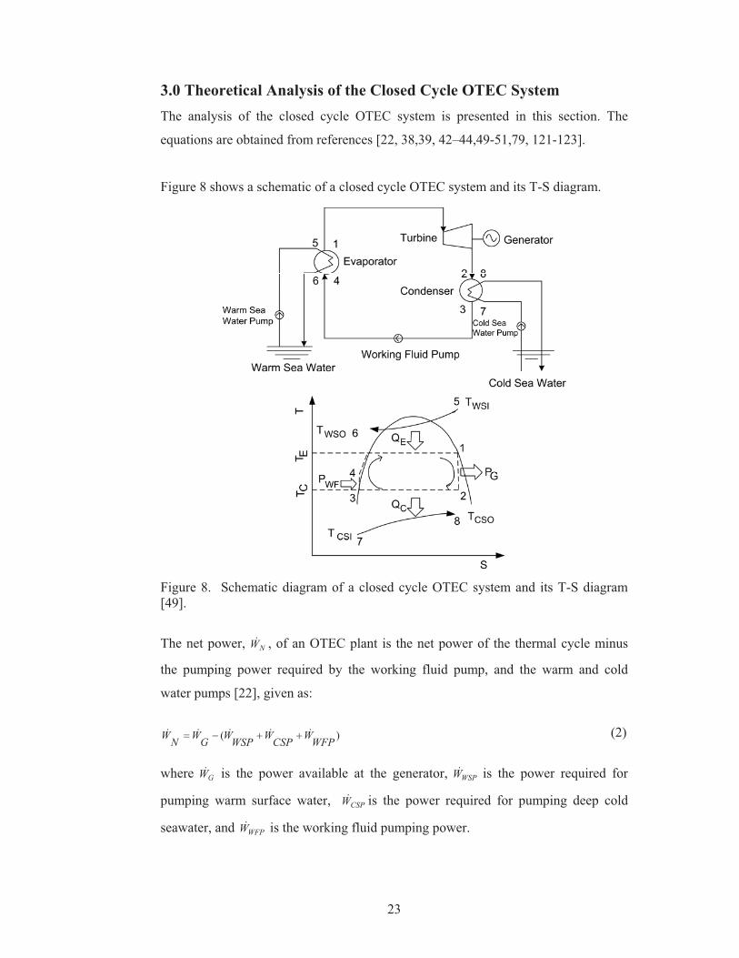
3.0 Theoretical Analysis of the Closed Cycle OTEC System The analysis of the closed cycle OTEC system is presented in this section. The

equations are obtained from references [22, 38,39, 42–44,49-51,79, 121-123].

Figure 8 shows a schematic of a closed cycle OTEC system and its T-S diagram.

Figure 8. Schematic diagram of a closed cycle OTEC system and its T-S diagram [49].

The net power, NW� , of an OTEC plant is the net power of the thermal cycle minus

the pumping power required by the working fluid pump, and the warm and cold

water pumps [22], given as:

)( WFPWCSPWWSPWGWNW ����� ���� (2)

where GW� is the power available at the generator, WSPW� is the power required for

pumping warm surface water, CSPW� is the power required for pumping deep cold

seawater, and WFPW� is the working fluid pumping power.

24

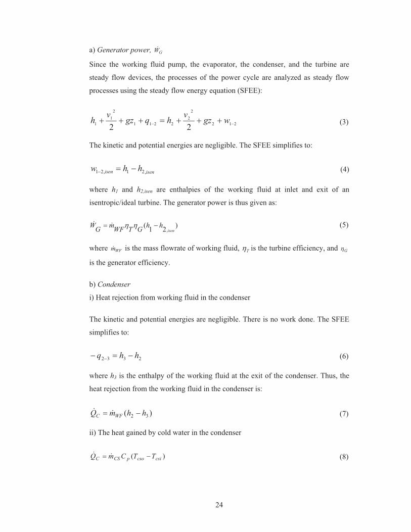
a) Generator power, GW�

Since the working fluid pump, the evaporator, the condenser, and the turbine are

steady flow devices, the processes of the power cycle are analyzed as steady flow

processes using the steady flow energy equation (SFEE):

212

22

2211

21

1 22 �� ������� wgzvhqgzvh (3)

The kinetic and potential energies are negligible. The SFEE simplifies to:

isenisen hhw ,21,21 ��� (4) where h1 and h2,isen are enthalpies of the working fluid at inlet and exit of an

isentropic/ideal turbine. The generator power is thus given as:

)21(

,isenhhGTWFmGW �� ���� (5)

where WFm� is the mass flowrate of working fluid, T� is the turbine efficiency, and G�

is the generator efficiency.

b) Condenser

i) Heat rejection from working fluid in the condenser

The kinetic and potential energies are negligible. There is no work done. The SFEE

simplifies to:

2332 hhq ��� � (6)

where h3 is the enthalpy of the working fluid at the exit of the condenser. Thus, the

heat rejection from the working fluid in the condenser is:

)( 32 hhmQ WFC �� �� (7)

ii) The heat gained by cold water in the condenser

)( csicsopCSC TTCmQ �� �� (8)

25

where CSm� is the mass flowrate of the deep cold sea water, pC is the specific heat,

csoT is the temperature of cold seawater at exit of condenser, and csiT is the cold sea

water temperature at inlet of condenser.

iii) The heat transfer in the condenser based on the heat transfer coefficient and the

log mean temperature difference is:

CmCCC TAUQ )(��� (9)

where CU is the overall heat transfer coefficient of the condenser, CA is the heat

transfer area of the condenser, and CmT )(� is the log mean temperature difference

(LMTD) of the condenser.

The log mean temperature difference is calculated as:

�

� �

��

�����

cso

csi

csocsiCm

TTTT

TTTTT

3

2

32

ln

)()()( (10)

where T2 and T3 are temperatures of the working fluid at the inlet and outlet of the

condenser.

c) Working fluid pump power, WFPW�

The kinetic and potential energies are negligible. Work is done on the pump,

therefore negative work output. SFEE simplifies to:

isenise hhw ,43,43 ��� � (11)

where h4,isen is the enthalpy of the working fluid at the exit of an isentropic/ideal

pump. The working fluid pump power is thus calculated as:

WFP

isenWFWFP

hhmW

�)( 3,4 �

��

� (12)

where WFP� is the working fluid pump efficiency. For real life analysis, the pump

efficiency should include the efficiency of the electric motor that runs the pump. The

shaft work for a steady flow device (pump) is:

26

���4

3

.dpvW (13)

The working fluid pumping power is also given as:

WFP

fWFWFP

PPvmW

�)( 34 ��

�� (14)

where fv is the specific volume of the working fluid, and 3P and 4P are operating

pressures.

d) Evaporator

i) Heat absorption by the working fluid in the evaporator

The kinetic and potential energies are negligible. There is no work done. The SFEE

simplifies to:

4114 hhq ��� (15)

The heat rejection from the working fluid in the evaporator is thus given as:

)( 41 hhmQ WFE �� �� (16)

ii) The heat loss by warm water in the evaporator

)( wsowsipWSE TTCmQ �� �� (17)

where WSm� is the mass flowrate of the warm surface sea water, pC is the specific

heat, wsiT is the temperature of warm seawater at inlet of evaporator, and WSOT is the

warm sea water temperature at outlet of evaporator.

iii) The heat transfer in the evaporator based on the heat transfer coefficient and the

log mean temperature difference is:

27

EmEEE TAUQ )(��� (18) where EU is the overall heat transfer coefficient of the evaporator, EA is the heat

transfer area of the evaporator, and EmT )(� is the log mean temperature difference

(LMTD) of the evaporator. The log mean temperature difference is calculated as:

�

� �

��

�����

4

1

41

ln

)()()(

TTTT

TTTTT

wso

wsi

wsowsiEm (19)

where T1 and T4 are temperatures of the working fluid at the inlet and outlet of the

evaporator.

e) Cold sea water pumping power, CSPW�

The cold seawater pumping power is given as:

CSP

CSPCSCSP

hgmW

��

��� (20)

where CSP� is the pump efficiency, g is the gravitational acceleration, and CSPh� is

the total head loss in the cold water pipe. The total head loss across the cold water

piping system is:

dCSCCSMCSSPCSCSP hhhhh )()()()( ��������� (21)

where (�hCS)SP, is the head loss due to friction in the straight cold water pipe, (�hCS)M

is the minor head losses due to bends, (�hCS)C is head loss of cold water in the

condenser, and (�hCS)d is the head loss due to density differences. The cold seawater

pumping power is thus given as:

� �

CSP

dCSCCSMCSSPCSCSCSP

hhhhgmW

�)()()()( �������

��� (22)

e) Warm sea water pumping power, WSPW�

The warm surface seawater pumping power is given as:

28

WSP

WSPWSWSP

hgmW

��

��� (23)

where WSP� is the pump efficiency, g is the gravitational acceleration, and WSPh� is

the total head loss in the warm water pipe. The total head loss across the warm water

piping system is:

EWSMWSSPWSWSP hhhh )()()( ������� (24)

where (�hWS)SP, is the frictional headloss in the straight warm water pipe, (�hWS)M is

the minor head losses in the pipe due to bends, and (�hWS)E, is the head loss of warm

water in the evaporator. The warm seawater pumping power is thus given as:

� �

WSP

EWSMWSSPWSWSWSP

hhhgmW

�)()()( �����

��� (25)

29

4.0 Device Designs, Fabrication, and Experimentation Experimental studies were conducted on a corrugated plate exchanger with varying

channel spacing, and a closed cycle OTEC demonstration plant. All the fabrications

and experiments were carried out in the thermo-fluids laboratory, the University of

the South Pacific.

4.1. Corrugated Plate Heat Exchanger

The current design is chosen based on the enhancement of heat transfer

characteristics due to the incorporation of wavy configurations in plate exchangers.

The traditional geometry of the wavy configurations is retained to reduce the number

of variables in the present work and to study the effect of the flow rate and plate

spacing. The hot water flowrates, HWV� , and the spacing between the plates, �X, are

varied while the corrugation pattern remain the same. The focus of the experiments is

on the measurements of the temperatures of the two fluids at inlet and exit of the heat

exchanger and then to determine which �X value gives optimum heat transfer. A

detailed physical explanation of the flow and the enhanced turbulence by the

corrugations in the channels is also presented.

Experiments were performed on a single corrugation pattern on twenty plates

arranged parallelly. The spacing between the plates, �X, was varied to

experimentally determine the spacing that gives the optimum heat transfer. Water

was used on both the hot and the cold channels with the flow being parallel. Both the

hot and cold water entered the heat exchanger from the bottom. This allowed the

water to fully fill the heat exchanger channels before exiting into the atmosphere,

thus utilizing the full area of the plates for effective heat transfer and preventing the

formation of hydraulic diameters. The flowrates, HWV� , for the hot side were varied

from 0.18L/s to 0.63 L/s, while the cold side flowrate, CWV� , was kept constant at

0.16L/s . The inlet temperatures for both the hot and cold water were kept constant at

49 ºC and 26 ºC respectively. This gives a temperature difference of 23 ºC at the inlet

of the heat exchanger. The plates used are corrugated galvanized sheets, with a

thickness of 0.4 mm. The other geometric details of the plates and the heat exchanger

are provided in Figure 9 and Table 1.

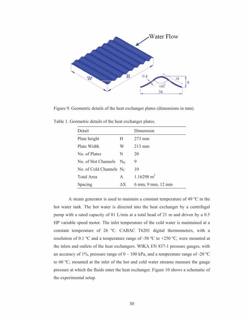
30

Figure 9. Geometric details of the heat exchanger plates (dimensions in mm).

Table 1. Geometric details of the heat exchanger plates.

Detail Dimension

Plate height H 273 mm

Plate Width W 213 mm

No. of Plates N 20

No. of Hot Channels NH 9

No. of Cold Channels NC 10

Total Area A 1.16298 m2

Spacing �X 6 mm, 9 mm, 12 mm

A steam generator is used to maintain a constant temperature of 49 ºC in the

hot water tank. The hot water is directed into the heat exchanger by a centrifugal

pump with a rated capacity of 81 L/min at a total head of 21 m and driven by a 0.5

HP variable speed motor. The inlet temperature of the cold water is maintained at a

constant temperature of 26 ºC. CABAC T6201 digital thermometers, with a

resolution of 0.1 ºC and a temperature range of -50 ºC to +250 ºC, were mounted at

the inlets and outlets of the heat exchangers. WIKA EN 837-1 pressure gauges, with

an accuracy of 1%, pressure range of 0 – 100 kPa, and a temperature range of -20 ºC

to 60 ºC, mounted at the inlet of the hot and cold water streams measure the gauge

pressure at which the fluids enter the heat exchanger. Figure 10 shows a schematic of

the experimental setup.

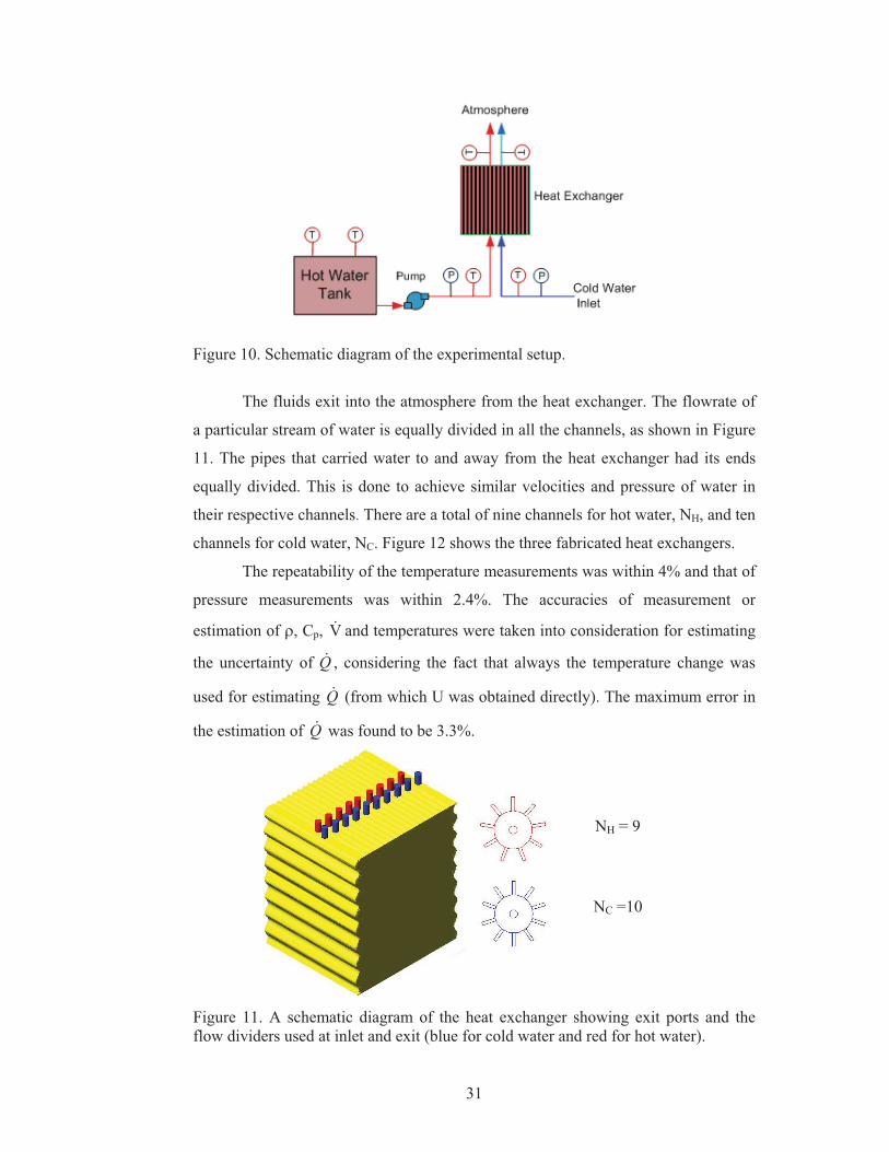
31

Figure 10. Schematic diagram of the experimental setup.

The fluids exit into the atmosphere from the heat exchanger. The flowrate of

a particular stream of water is equally divided in all the channels, as shown in Figure

11. The pipes that carried water to and away from the heat exchanger had its ends

equally divided. This is done to achieve similar velocities and pressure of water in

their respective channels. There are a total of nine channels for hot water, NH, and ten

channels for cold water, NC. Figure 12 shows the three fabricated heat exchangers.

The repeatability of the temperature measurements was within 4% and that of

pressure measurements was within 2.4%. The accuracies of measurement or

estimation of �, Cp, V� and temperatures were taken into consideration for estimating

the uncertainty of Q� , considering the fact that always the temperature change was

used for estimating Q� (from which U was obtained directly). The maximum error in

the estimation of Q� was found to be 3.3%.

Figure 11. A schematic diagram of the heat exchanger showing exit ports and the flow dividers used at inlet and exit (blue for cold water and red for hot water).

NH = 9

NC =10

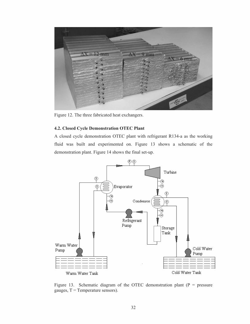
32

Figure 12. The three fabricated heat exchangers.

4.2. Closed Cycle Demonstration OTEC Plant

A closed cycle demonstration OTEC plant with refrigerant R134-a as the working

fluid was built and experimented on. Figure 13 shows a schematic of the

demonstration plant. Figure 14 shows the final set-up.

Figure 13. Schematic diagram of the OTEC demonstration plant (P = pressure gauges, T = Temperature sensors).

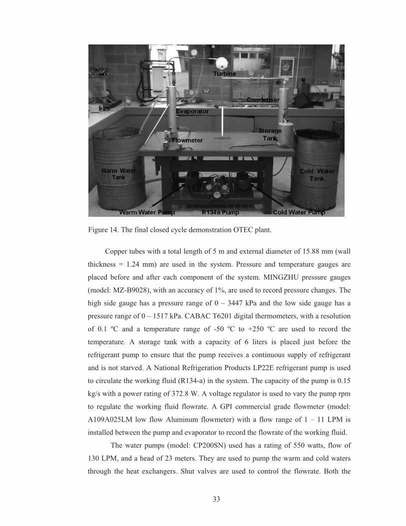
33

Figure 14. The final closed cycle demonstration OTEC plant.

Copper tubes with a total length of 5 m and external diameter of 15.88 mm (wall

thickness = 1.24 mm) are used in the system. Pressure and temperature gauges are

placed before and after each component of the system. MINGZHU pressure gauges

(model: MZ-B9028), with an accuracy of 1%, are used to record pressure changes. The

high side gauge has a pressure range of 0 – 3447 kPa and the low side gauge has a

pressure range of 0 – 1517 kPa. CABAC T6201 digital thermometers, with a resolution

of 0.1 ºC and a temperature range of -50 ºC to +250 ºC are used to record the

temperature. A storage tank with a capacity of 6 liters is placed just before the

refrigerant pump to ensure that the pump receives a continuous supply of refrigerant

and is not starved. A National Refrigeration Products LP22E refrigerant pump is used

to circulate the working fluid (R134-a) in the system. The capacity of the pump is 0.15

kg/s with a power rating of 372.8 W. A voltage regulator is used to vary the pump rpm

to regulate the working fluid flowrate. A GPI commercial grade flowmeter (model:

A109A025LM low flow Aluminum flowmeter) with a flow range of 1 – 11 LPM is

installed between the pump and evaporator to record the flowrate of the working fluid.

The water pumps (model: CP200SN) used has a rating of 550 watts, flow of

130 LPM, and a head of 23 meters. They are used to pump the warm and cold waters

through the heat exchangers. Shut valves are used to control the flowrate. Both the

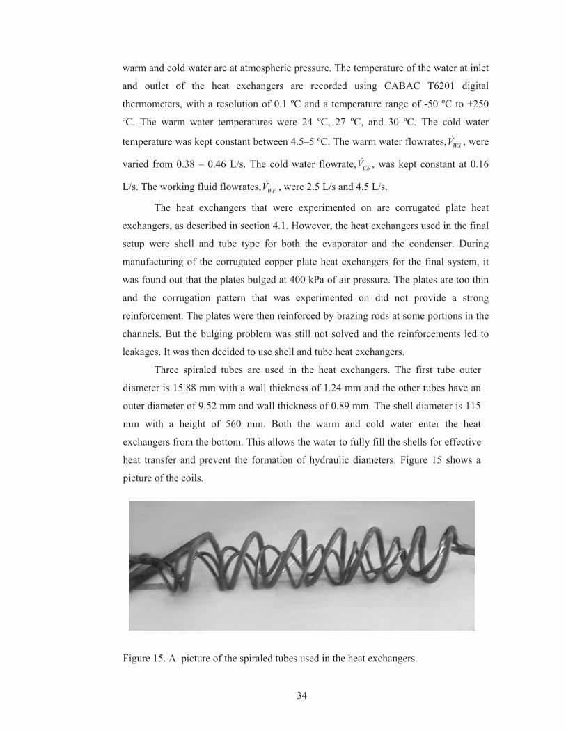
34

warm and cold water are at atmospheric pressure. The temperature of the water at inlet

and outlet of the heat exchangers are recorded using CABAC T6201 digital

thermometers, with a resolution of 0.1 ºC and a temperature range of -50 ºC to +250

ºC. The warm water temperatures were 24 ºC, 27 ºC, and 30 ºC. The cold water

temperature was kept constant between 4.5–5 ºC. The warm water flowrates, WSV� , were

varied from 0.38 – 0.46 L/s. The cold water flowrate, CSV� , was kept constant at 0.16

L/s. The working fluid flowrates, WFV� , were 2.5 L/s and 4.5 L/s.

The heat exchangers that were experimented on are corrugated plate heat

exchangers, as described in section 4.1. However, the heat exchangers used in the final

setup were shell and tube type for both the evaporator and the condenser. During

manufacturing of the corrugated copper plate heat exchangers for the final system, it

was found out that the plates bulged at 400 kPa of air pressure. The plates are too thin

and the corrugation pattern that was experimented on did not provide a strong

reinforcement. The plates were then reinforced by brazing rods at some portions in the

channels. But the bulging problem was still not solved and the reinforcements led to

leakages. It was then decided to use shell and tube heat exchangers.

Three spiraled tubes are used in the heat exchangers. The first tube outer

diameter is 15.88 mm with a wall thickness of 1.24 mm and the other tubes have an

outer diameter of 9.52 mm and wall thickness of 0.89 mm. The shell diameter is 115

mm with a height of 560 mm. Both the warm and cold water enter the heat

exchangers from the bottom. This allows the water to fully fill the shells for effective

heat transfer and prevent the formation of hydraulic diameters. Figure 15 shows a

picture of the coils.

Figure 15. A picture of the spiraled tubes used in the heat exchangers.

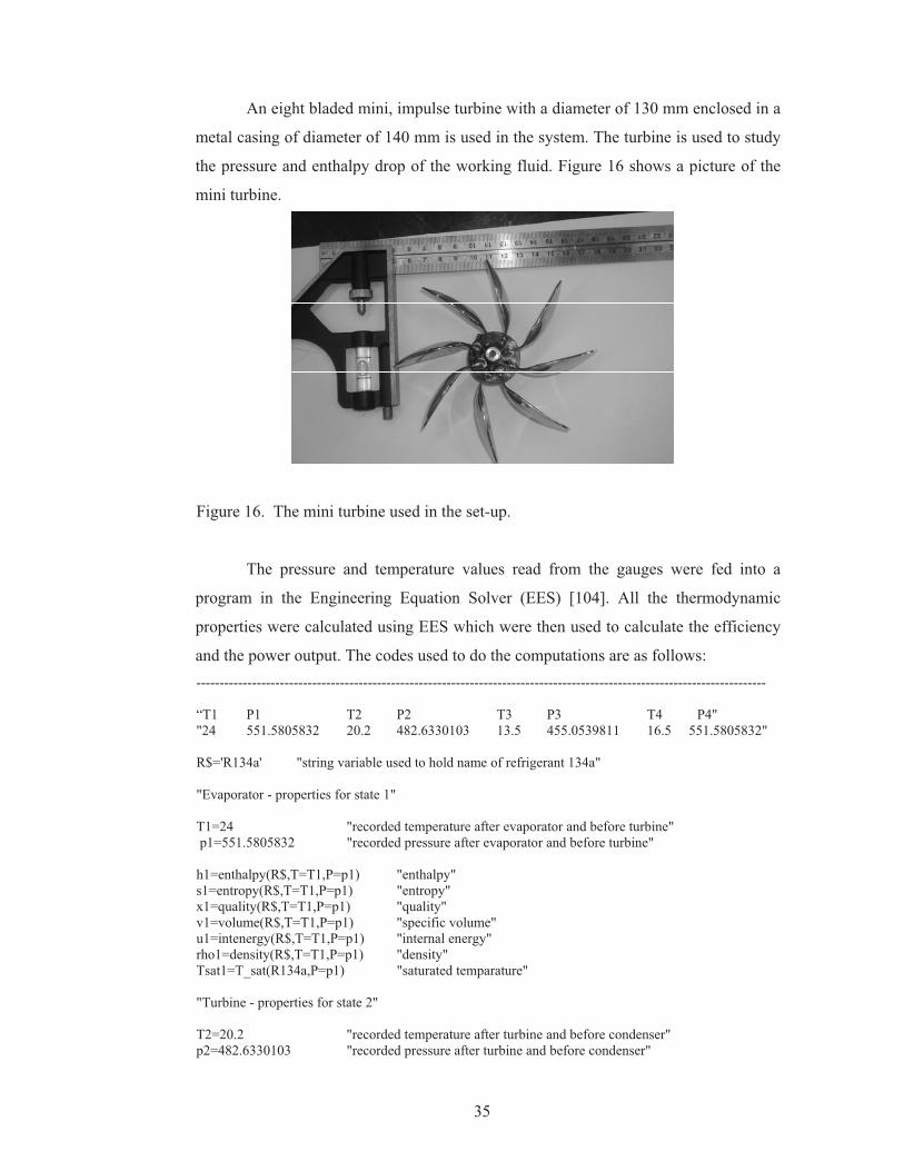
35

An eight bladed mini, impulse turbine with a diameter of 130 mm enclosed in a

metal casing of diameter of 140 mm is used in the system. The turbine is used to study

the pressure and enthalpy drop of the working fluid. Figure 16 shows a picture of the

mini turbine.

Figure 16. The mini turbine used in the set-up.

The pressure and temperature values read from the gauges were fed into a

program in the Engineering Equation Solver (EES) [104]. All the thermodynamic

properties were calculated using EES which were then used to calculate the efficiency

and the power output. The codes used to do the computations are as follows: --------------------------------------------------------------------------------------------------------------------------- “T1 P1 T2 P2 T3 P3 T4 P4" "24 551.5805832 20.2 482.6330103 13.5 455.0539811 16.5 551.5805832" R$='R134a' "string variable used to hold name of refrigerant 134a" "Evaporator - properties for state 1" T1=24 "recorded temperature after evaporator and before turbine" p1=551.5805832 "recorded pressure after evaporator and before turbine" h1=enthalpy(R$,T=T1,P=p1) "enthalpy" s1=entropy(R$,T=T1,P=p1) "entropy" x1=quality(R$,T=T1,P=p1) "quality" v1=volume(R$,T=T1,P=p1) "specific volume" u1=intenergy(R$,T=T1,P=p1) "internal energy" rho1=density(R$,T=T1,P=p1) "density" Tsat1=T_sat(R134a,P=p1) "saturated temparature" "Turbine - properties for state 2" T2=20.2 "recorded temperature after turbine and before condenser" p2=482.6330103 "recorded pressure after turbine and before condenser"

36

h2=enthalpy(R$,T=T2,P=p2) s2=entropy(R$,T=T2,P=p2) x2=quality(R$,T=T2,P=p2) v2=volume(R$,T=T2,P=p2) u2=intenergy(R$,T=T2,P=p2) rho2=density(R$,T=T2,P=p2) Tsat2=T_sat(R134a,P=p2) "Condenser - properties for state 3" T3=13.5 "recorded temperature after condenser and before pump" p3=455.0539811 "recorded pressure after condenser and before pump" h3=enthalpy(R$,T=T3,P=p3) s3=entropy(R$,T=T3,P=p3) x3=quality(R$,T=T3,P=p3) v3=volume(R$,T=T3,P=p3) u3=intenergy(R$,T=T3,P=p3) rho3=density(R$,T=T3,P=p3) Tsat3=T_sat(R134a,P=p3) "Pump - properties for state 4" T4=16.5 "recorded temperature after pump and before evaporator" p4=551.5805832 "recorded pressure after pump and before evaporator" h4=enthalpy(R$,T=T4,P=p4) s4=entropy(R$,T=T4,P=p4) x4=quality(R$,T=T4,P=p4) v4=volume(R$,T=T4,P=p4) u4=intenergy(R$,T=T4,P=p4) rho4=density(R$,T=T4,P=p4) Tsat4=T_sat(R134a,P=p4) $TabWidth 2 cm ---------------------------------------------------------------------------------------------------------------------------

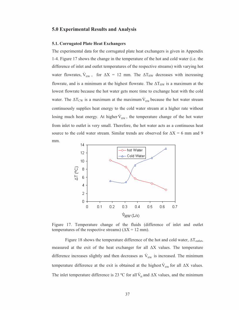
37

5.0 Experimental Results and Analysis

5.1. Corrugated Plate Heat Exchangers

The experimental data for the corrugated plate heat exchangers is given in Appendix

1-4. Figure 17 shows the change in the temperature of the hot and cold water (i.e. the

difference of inlet and outlet temperatures of the respective streams) with varying hot

water flowrates, HWV� , for �X = 12 mm. The �THW decreases with increasing

flowrate, and is a minimum at the highest flowrate. The �THW is a maximum at the

lowest flowrate because the hot water gets more time to exchange heat with the cold

water. The �TCW is a maximum at the maximum HWV� because the hot water stream

continuously supplies heat energy to the cold water stream at a higher rate without

losing much heat energy. At higher HWV� , the temperature change of the hot water

from inlet to outlet is very small. Therefore, the hot water acts as a continuous heat

source to the cold water stream. Similar trends are observed for �X = 6 mm and 9

mm.

Figure 17. Temperature change of the fluids (difference of inlet and outlet temperatures of the respective streams) (�X = 12 mm).

Figure 18 shows the temperature difference of the hot and cold water, �Toutlet,

measured at the exit of the heat exchanger for all �X values. The temperature

difference increases slightly and then decreases as HWV� is increased. The minimum

temperature difference at the exit is obtained at the highest HWV� for all �X values.

The inlet temperature difference is 23 ºC for all HV� and �X values, and the minimum

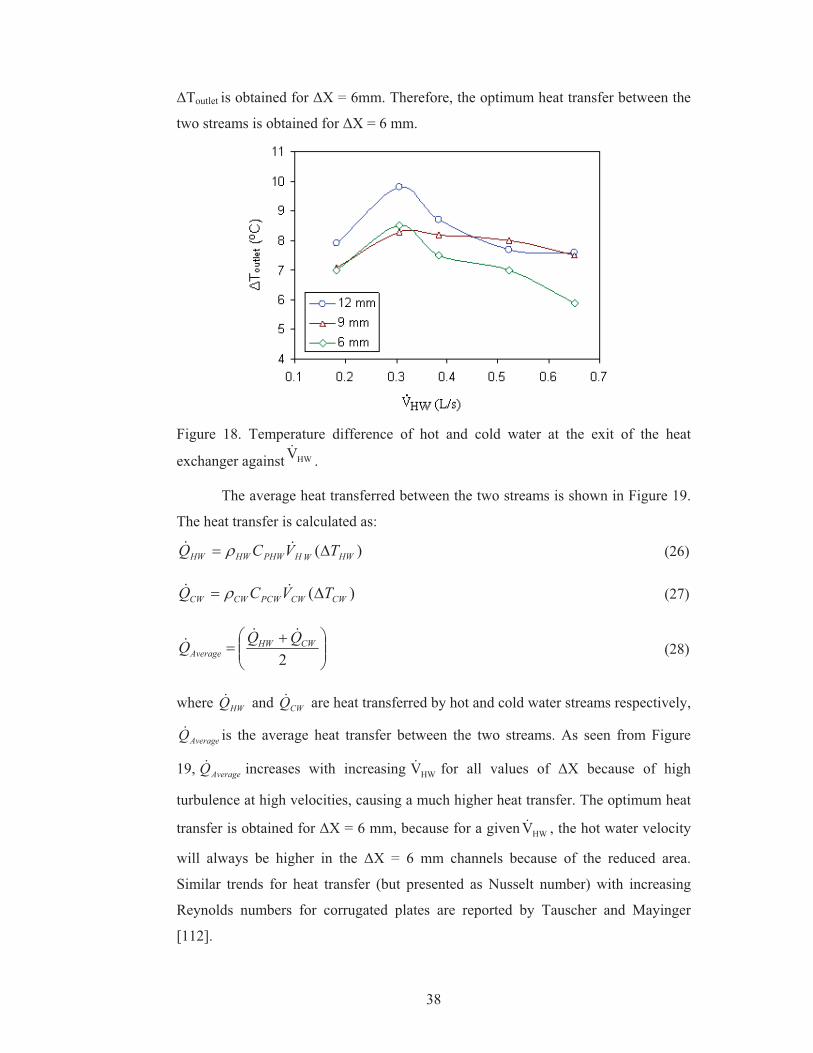
38

�Toutlet is obtained for �X = 6mm. Therefore, the optimum heat transfer between the

two streams is obtained for �X = 6 mm.

Figure 18. Temperature difference of hot and cold water at the exit of the heat

exchanger against HWV� .

The average heat transferred between the two streams is shown in Figure 19.

The heat transfer is calculated as:

)( HWWHPHWHWHW TVCQ �� �� � (26)

)( CWCWPCWCWCW TVCQ �� �� � (27)

���

����

� ��

2CWHW

AverageQQQ��

� (28)

where HWQ� and CWQ� are heat transferred by hot and cold water streams respectively,

AverageQ� is the average heat transfer between the two streams. As seen from Figure

19, AverageQ� increases with increasing HWV� for all values of �X because of high

turbulence at high velocities, causing a much higher heat transfer. The optimum heat

transfer is obtained for �X = 6 mm, because for a given HWV� , the hot water velocity

will always be higher in the �X = 6 mm channels because of the reduced area.

Similar trends for heat transfer (but presented as Nusselt number) with increasing

Reynolds numbers for corrugated plates are reported by Tauscher and Mayinger

[112].

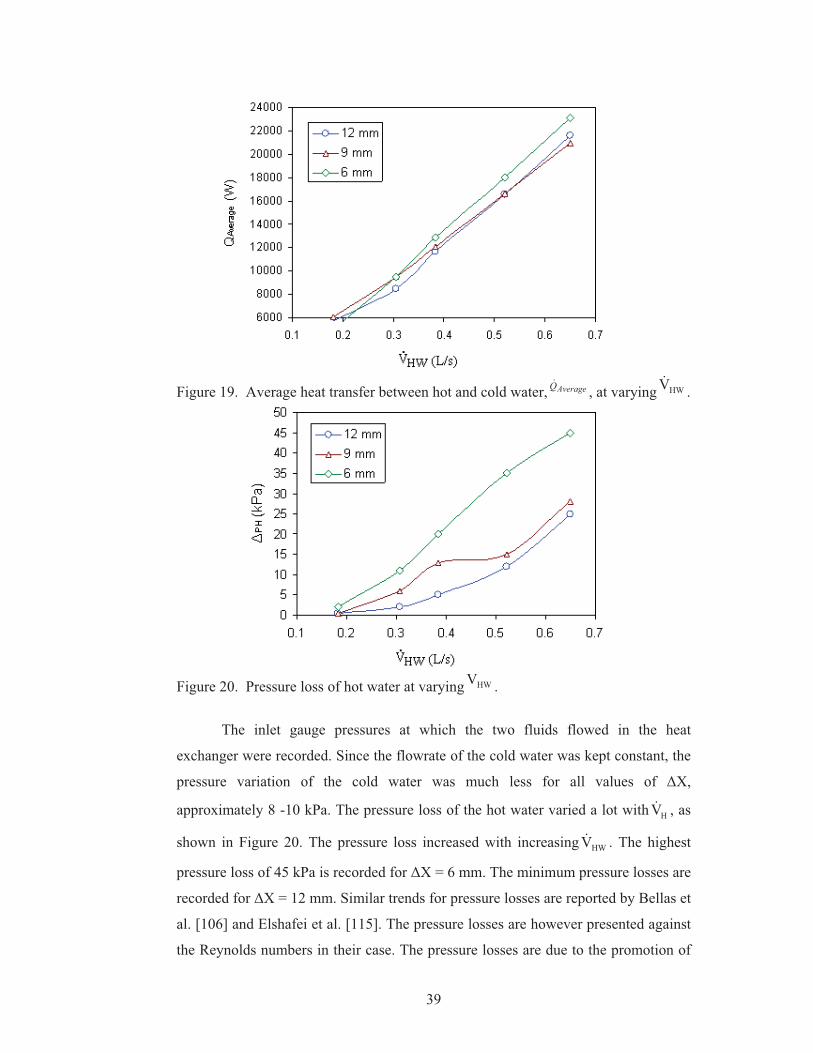
39

Figure 19. Average heat transfer between hot and cold water, AverageQ� , at varying HWV� .

Figure 20. Pressure loss of hot water at varying HWV� .

The inlet gauge pressures at which the two fluids flowed in the heat

exchanger were recorded. Since the flowrate of the cold water was kept constant, the

pressure variation of the cold water was much less for all values of �X,

approximately 8 -10 kPa. The pressure loss of the hot water varied a lot with HV� , as

shown in Figure 20. The pressure loss increased with increasing HWV� . The highest

pressure loss of 45 kPa is recorded for �X = 6 mm. The minimum pressure losses are

recorded for �X = 12 mm. Similar trends for pressure losses are reported by Bellas et

al. [106] and Elshafei et al. [115]. The pressure losses are however presented against

the Reynolds numbers in their case. The pressure losses are due to the promotion of

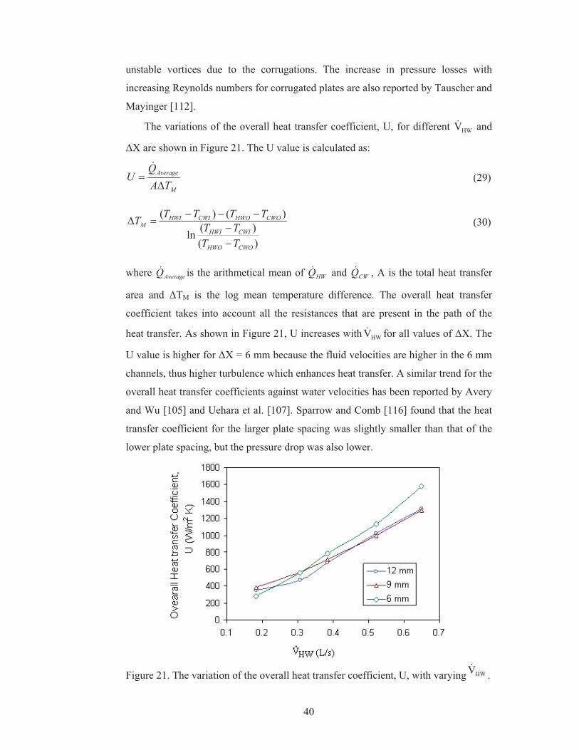
40

unstable vortices due to the corrugations. The increase in pressure losses with

increasing Reynolds numbers for corrugated plates are also reported by Tauscher and

Mayinger [112].

The variations of the overall heat transfer coefficient, U, for different HWV� and

�X are shown in Figure 21. The U value is calculated as:

M

Average

TAQ

U�

��

(29)

)()(ln

)()(

CWOHWO

CWIHWI

CWOHWOCWIHWIM

TTTT

TTTTT

��

����� (30)

where AverageQ� is the arithmetical mean of HWQ� and CWQ� , A is the total heat transfer

area and �TM is the log mean temperature difference. The overall heat transfer

coefficient takes into account all the resistances that are present in the path of the

heat transfer. As shown in Figure 21, U increases with HWV� for all values of �X. The

U value is higher for �X = 6 mm because the fluid velocities are higher in the 6 mm

channels, thus higher turbulence which enhances heat transfer. A similar trend for the

overall heat transfer coefficients against water velocities has been reported by Avery

and Wu [105] and Uehara et al. [107]. Sparrow and Comb [116] found that the heat

transfer coefficient for the larger plate spacing was slightly smaller than that of the

lower plate spacing, but the pressure drop was also lower.

Figure 21. The variation of the overall heat transfer coefficient, U, with varying HWV� .

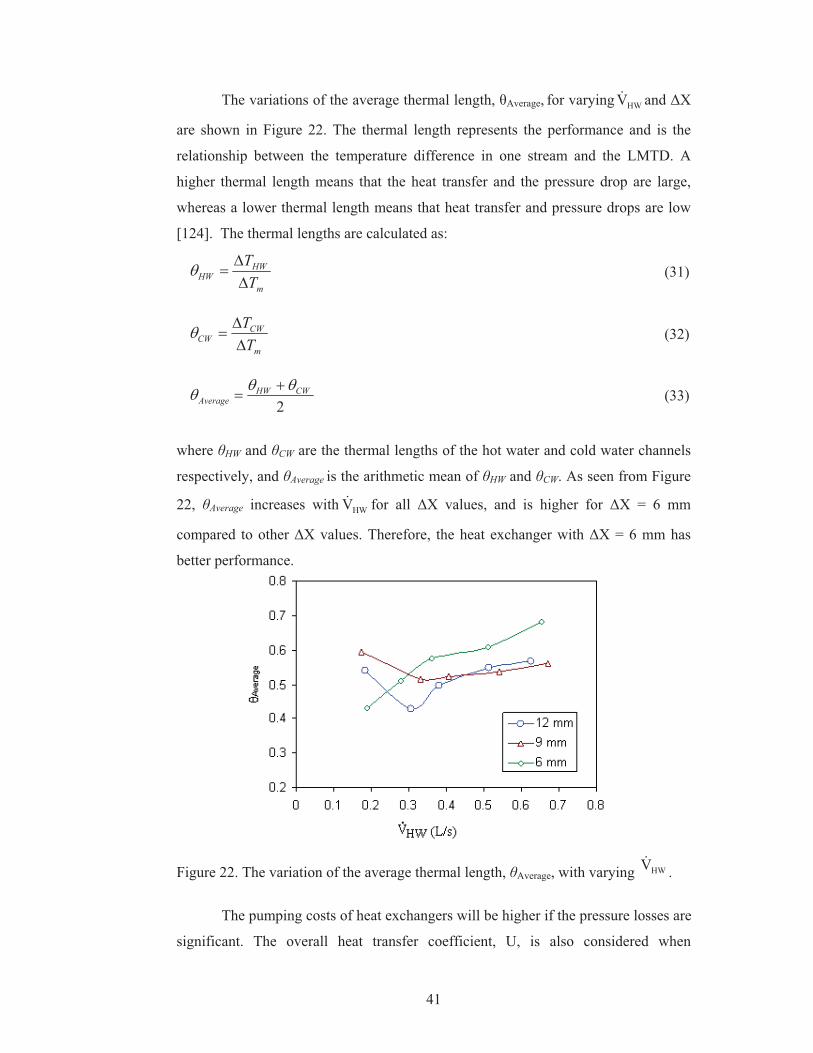
41

The variations of the average thermal length, �Average, for varying HWV� and �X

are shown in Figure 22. The thermal length represents the performance and is the

relationship between the temperature difference in one stream and the LMTD. A

higher thermal length means that the heat transfer and the pressure drop are large,

whereas a lower thermal length means that heat transfer and pressure drops are low

[124]. The thermal lengths are calculated as:

m

HWHW T

T��

�� (31)

m

CWCW T

T��

�� (32)

2

CWHWAverage

��� �� (33)

where �HW and �CW are the thermal lengths of the hot water and cold water channels

respectively, and �Average is the arithmetic mean of �HW and �CW. As seen from Figure

22, �Average increases with HWV� for all �X values, and is higher for �X = 6 mm

compared to other �X values. Therefore, the heat exchanger with �X = 6 mm has

better performance.

Figure 22. The variation of the average thermal length, �Average, with varying HWV� .

The pumping costs of heat exchangers will be higher if the pressure losses are

significant. The overall heat transfer coefficient, U, is also considered when

42

designing or choosing heat exchangers. Figure 23 shows a relationship between the

U value and the pressure losses of the warm water for all values of �X. A similar

criterion for the selection of heat exchangers based on the heat transfer coefficient

and the pressure losses is reported by Rafferty and Culver [108]. There is an increase

in the U value with increasing pressure loss. For �X = 6 mm, there is a high pressure

loss, therefore, the heat exchanger would have higher operational costs. However, the

heat exchanger with �X = 6 mm is appropriate because of significant heat transfer

coefficients and effective heat transfer, even though the pressure losses are higher.

The operational cost could be higher due to high pressure losses, but the main

objective is to obtain an effective heat transfer rate between the two streams for such

a low temperature difference.

Figure 23. The overall heat transfer coefficient, U, presented against the pressure loss of the hot water, �PH.

Both the hot and cold water streams are single-phase flows that undergo

mainly forced convection and conduction in the heat exchanger channels. A

hydrodynamic and a thermal boundary layer begin to develop as soon as the fluids

enter the channels. The convex and concave surfaces in the closed channels cause

instabilities in the flow, which enhance turbulence. The flow over the convex surface

is more stable because the velocity gradient maintains a constant sign across the

boundary layer [125], and any fluid element that gets displaced outward to a higher

velocity region gets pushed back to a lower radius region due to higher radial

pressure gradient [126]. The flow over the concave surface is unstable because the

velocity gradient changes sign in the boundary layer [125], and any fluid element

43

that gets displaced to a greater radius moves into a region of low velocities where the

pressure gradient is too low to push it back to a lower radius (Görtler instability)

[126]. The secondary flows or the Görtler vortices induced by the corrugations cause

the partial restarts of the boundary layer [111], and prevent it from being fully

developed.

The boundary layer over the convex surface has a point of inflection which

slows down the flow near the surface and changes the flow direction under a strong

adverse pressure gradient. When the incoming flow meets the reversed flow at some

point, the fluid near the surface is transported into the mainstream, or separated from

the surface. Since the flow is in a closed channel, and the plate geometries are same,

most of the fluid elements are pushed back to the surface. However, due to initial

separation, there are vortices formed in the wake region and their characteristics

depend on the Reynolds numbers. When on the concave surface, the flow gets

unstable due to Görtler instability. As the flow moves forward, it encounters a rising

wall (the next convex surface) and as a result, the flow close to the wall slows down

and disturbs the incoming flow. As a result, turbulence is enhanced and this

continues upto the end of the channel. Metwally and Manglik [127] performed a

numerical study on sinusoidal plate channels and concluded that flow separation and

attachment generates vortices that cause mixing which enhances the heat transfer.

The corrugations on the plates always cause turbulence in the channels regardless of

the flow being laminar or turbulent at the entrance of the channels. Turbulence in the

channels leads to wall shear stresses which also reduces fouling on the plate surfaces.

The heat transfer is a result of the disruptions of both the hydrodynamic and the

thermal boundary layers.

Smooth plates are not so effective because once the hydraulic boundary layer

is fully developed, the central region of the fluids do not receive much heat from the

adjacent channel compared to the fluid elements close to the wall. Also, as the wall

spacing is increased, the heat received by the central region decreases. In contrast,

corrugations on the plate surface lead to continuous disruptions in the boundary layer

across the length of a channel from inlet to exit. The secondary flow causes turbulent

mixing of the fluids in the channels from one wall to another. This allows almost all

the fluid elements to have effective heat transfer from adjacent channels. Therefore,

it is advisable to always prefer corrugated plates over smooth plates for plate type

heat exchangers.

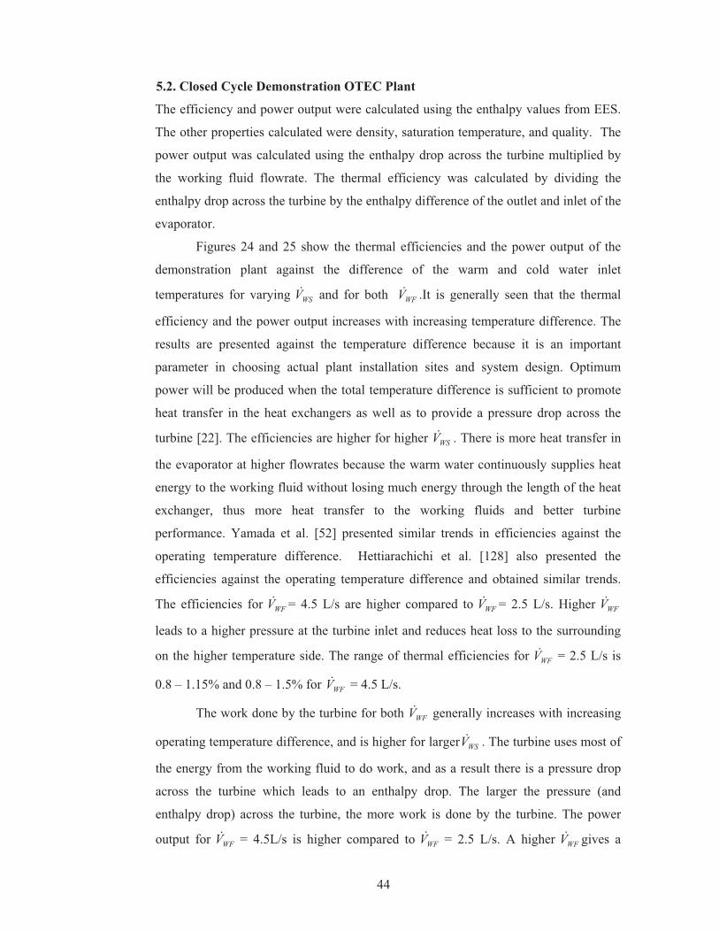
44

5.2. Closed Cycle Demonstration OTEC Plant

The efficiency and power output were calculated using the enthalpy values from EES.

The other properties calculated were density, saturation temperature, and quality. The

power output was calculated using the enthalpy drop across the turbine multiplied by

the working fluid flowrate. The thermal efficiency was calculated by dividing the

enthalpy drop across the turbine by the enthalpy difference of the outlet and inlet of the

evaporator.

Figures 24 and 25 show the thermal efficiencies and the power output of the

demonstration plant against the difference of the warm and cold water inlet

temperatures for varying WSV� and for both WFV� .It is generally seen that the thermal

efficiency and the power output increases with increasing temperature difference. The

results are presented against the temperature difference because it is an important

parameter in choosing actual plant installation sites and system design. Optimum

power will be produced when the total temperature difference is sufficient to promote

heat transfer in the heat exchangers as well as to provide a pressure drop across the

turbine [22]. The efficiencies are higher for higher WSV� . There is more heat transfer in

the evaporator at higher flowrates because the warm water continuously supplies heat

energy to the working fluid without losing much energy through the length of the heat

exchanger, thus more heat transfer to the working fluids and better turbine

performance. Yamada et al. [52] presented similar trends in efficiencies against the

operating temperature difference. Hettiarachichi et al. [128] also presented the

efficiencies against the operating temperature difference and obtained similar trends.

The efficiencies for WFV� = 4.5 L/s are higher compared to WFV� = 2.5 L/s. Higher WFV�

leads to a higher pressure at the turbine inlet and reduces heat loss to the surrounding

on the higher temperature side. The range of thermal efficiencies for WFV� = 2.5 L/s is

0.8 – 1.15% and 0.8 – 1.5% for WFV� = 4.5 L/s.

The work done by the turbine for both WFV� generally increases with increasing

operating temperature difference, and is higher for larger WSV� . The turbine uses most of

the energy from the working fluid to do work, and as a result there is a pressure drop

across the turbine which leads to an enthalpy drop. The larger the pressure (and

enthalpy drop) across the turbine, the more work is done by the turbine. The power

output for WFV� = 4.5L/s is higher compared to WFV� = 2.5 L/s. A higher WFV� gives a

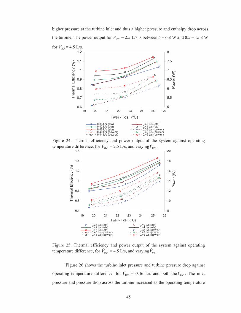
45

higher pressure at the turbine inlet and thus a higher pressure and enthalpy drop across

the turbine. The power output for WFV� = 2.5 L/s is between 5 – 6.8 W and 8.5 – 15.8 W

for WFV� = 4.5 L/s.

Figure 24. Thermal efficiency and power output of the system against operating temperature difference, for WFV� = 2.5 L/s, and varying WSV� .

Figure 25. Thermal efficiency and power output of the system against operating temperature difference, for WFV� = 4.5 L/s, and varying WSV� .

Figure 26 shows the turbine inlet pressure and turbine pressure drop against

operating temperature difference, for WSV� = 0.46 L/s and both the WFV� . The inlet

pressure and pressure drop across the turbine increased as the operating temperature

0.4

0.6

0.8

1

1.2

1.4

1.6

19 20 21 22 23 24 25 26Twsi - Tcsi (ºC)

Ther

mal

Effi

cien

cy (%

)

8

10

12

14

16

18

20

Pow

er (W

)

0.38 L/s (eta) 0.40 L/s (eta)0.42 L/s (eta) 0.44 L/s (eta)0.46 L/s (eta) 0.38 L/s (pow er)0.40 L/s (pow er) 0.42 L/s (pow er)0.44 L/s (pow er) 0.46 L/s (pow er)

0.6

0.7

0.8

0.9

1

1.1

1.2

19 20 21 22 23 24 25 26

Twsi - Tcsi (ºC)

Ther

mal

Effi

cien

cy (%

)

5

5.5

6

6.5

7

7.5

8

Pow

er (W

)

0.38 L/s (eta) 0.40 L/s (eta)0.42 L/s (eta) 0.44 L/s (eta)0.46 L/s (eta) 0.38 L/s (pow er)0.40 L/s (pow er) 0.42 L/s (pow er)0.44 L/s (pow er) 0.46 L/s (pow er)

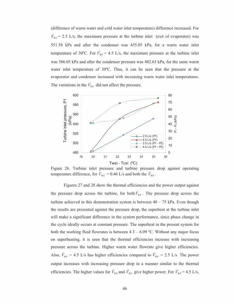
46

480

500

520

540

560

580

600

19 20 21 22 23 24 25 26

Twsi - Tcsi (ºC)

Turb

ine

inle

t pre

ssur

e, P

1 (k

Pa)

0

10

20

30

40

50

60

70

80

P 1 -

P 2 (k

Pa)

2.5 L/s (P1)4.5 L/s (P1)2.5 L/s (P1 - P2)4.5 L/s (P1 - P2)

(difference of warm water and cold water inlet temperature) difference increased. For

WFV� = 2.5 L/s, the maximum pressure at the turbine inlet (exit of evaporator) was

551.58 kPa and after the condenser was 455.05 kPa, for a warm water inlet

temperature of 30ºC. For WFV� = 4.5 L/s, the maximum pressure at the turbine inlet

was 586.05 kPa and after the condenser pressure was 482.63 kPa, for the same warm

water inlet temperature of 30ºC. Thus, it can be seen that the pressure at the

evaporator and condenser increased with increasing warm water inlet temperatures.

The variations in the WSV� did not affect the pressure.

Figure 26. Turbine inlet pressure and turbine pressure drop against operating temperature difference, for WSV� = 0.46 L/s and both the WFV� .

Figures 27 and 28 show the thermal efficiencies and the power output against

the pressure drop across the turbine, for both WFV� . The pressure drop across the

turbine achieved in this demonstration system is between 40 – 75 kPa. Even though

the results are presented against the pressure drop, the superheat at the turbine inlet

will make a significant difference in the system performance, since phase change in

the cycle ideally occurs at constant pressure. The superheat in the present system for

both the working fluid flowrates is between 4.3 – 6.09 ºC. Without any major focus

on superheating, it is seen that the thermal efficiencies increase with increasing

pressure across the turbine. Higher warm water flowrate give higher efficiencies.

Also, WFV� = 4.5 L/s has higher efficiencies compared to WFV� = 2.5 L/s. The power

output increases with increasing pressure drop in a manner similar to the thermal

efficiencies. The higher values for WSV� and WFV� give higher power. For WFV� = 4.5 L/s,

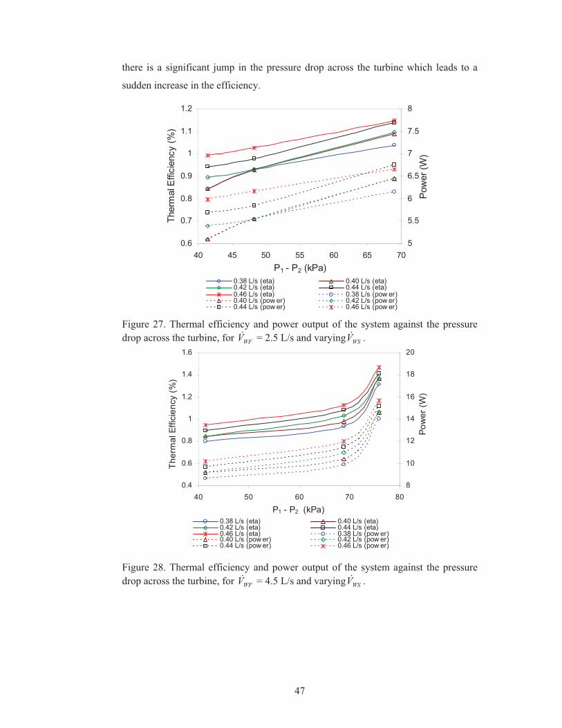
47

there is a significant jump in the pressure drop across the turbine which leads to a

sudden increase in the efficiency.

Figure 27. Thermal efficiency and power output of the system against the pressure drop across the turbine, for WFV� = 2.5 L/s and varying WSV� .

Figure 28. Thermal efficiency and power output of the system against the pressure drop across the turbine, for WFV� = 4.5 L/s and varying WSV� .

0.4

0.6

0.8

1

1.2

1.4

1.6

40 50 60 70 80

P1 - P2 (kPa)

Ther

mal

Effi

cien

cy (%

)

8

10

12

14

16

18

20

Pow

er (W

)

0.38 L/s (eta) 0.40 L/s (eta)0.42 L/s (eta) 0.44 L/s (eta)0.46 L/s (eta) 0.38 L/s (pow er)0.40 L/s (pow er) 0.42 L/s (pow er)0.44 L/s (pow er) 0.46 L/s (pow er)

0.6

0.7

0.8

0.9

1

1.1

1.2

40 45 50 55 60 65 70P1 - P2 (kPa)

Ther

mal

Effi

cien

cy (%

)

5

5.5

6

6.5

7

7.5

8

Pow

er (W

)

0.38 L/s (eta) 0.40 L/s (eta)0.42 L/s (eta) 0.44 L/s (eta)0.46 L/s (eta) 0.38 L/s (pow er)0.40 L/s (pow er) 0.42 L/s (pow er)0.44 L/s (pow er) 0.46 L/s (pow er)

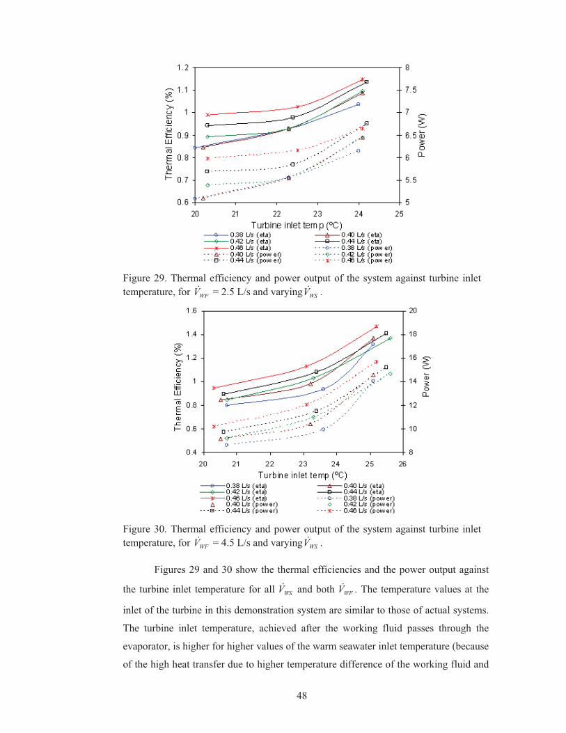
48

Figure 29. Thermal efficiency and power output of the system against turbine inlet temperature, for WFV� = 2.5 L/s and varying WSV� .

Figure 30. Thermal efficiency and power output of the system against turbine inlet temperature, for WFV� = 4.5 L/s and varying WSV� .

Figures 29 and 30 show the thermal efficiencies and the power output against

the turbine inlet temperature for all WSV� and both WFV� . The temperature values at the

inlet of the turbine in this demonstration system are similar to those of actual systems.

The turbine inlet temperature, achieved after the working fluid passes through the

evaporator, is higher for higher values of the warm seawater inlet temperature (because

of the high heat transfer due to higher temperature difference of the working fluid and

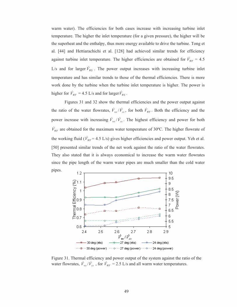
49

warm water). The efficiencies for both cases increase with increasing turbine inlet

temperature. The higher the inlet temperature (for a given pressure), the higher will be

the superheat and the enthalpy, thus more energy available to drive the turbine. Tong et

al. [44] and Hettiarachichi et al. [128] had achieved similar trends for efficiency

against turbine inlet temperature. The higher efficiencies are obtained for WFV� = 4.5

L/s and for larger WSV� . The power output increases with increasing turbine inlet

temperature and has similar trends to those of the thermal efficiencies. There is more

work done by the turbine when the turbine inlet temperature is higher. The power is

higher for WFV� = 4.5 L/s and for larger WSV� .

Figures 31 and 32 show the thermal efficiencies and the power output against

the ratio of the water flowrates, wsV� / csV� , for both WFV� . Both the efficiency and the

power increase with increasing wsV� / csV� . The highest efficiency and power for both

WFV� are obtained for the maximum water temperature of 30ºC. The higher flowrate of

the working fluid ( WFV� = 4.5 L/s) gives higher efficiencies and power output. Yeh et al.

[50] presented similar trends of the net work against the ratio of the water flowrates.

They also stated that it is always economical to increase the warm water flowrates

since the pipe length of the warm water pipes are much smaller than the cold water

pipes.

Figure 31. Thermal efficiency and power output of the system against the ratio of the water flowrates, wsV� / csV� , for WFV� = 2.5 L/s and all warm water temperatures.

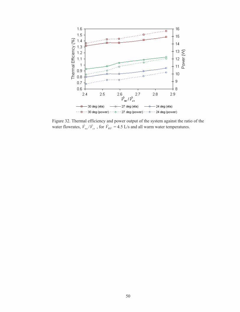
50

Figure 32. Thermal efficiency and power output of the system against the ratio of the water flowrates, wsV� / csV� , for WFV� = 4.5 L/s and all warm water temperatures.

51

6.0 Conclusions The heat exchange processes across the ocean surface and the technology for ocean

thermal energy conversion are presented. The heat exchange processes across the

ocean surface are represented in an ocean energy budget. Ocean currents transfer

thermal energy from the lower latitudes to cooler regions in the higher latitudes. The

ocean energy budget quantifies the amount of heat gained and lost by the ocean, and

this can be used to determine the overall temperature change of the system over a

certain period of time. The accurate measurements and predictions of the ocean

energy budget terms are difficult and some errors and imbalances are still present.

The transport of cold water from the higher latitudes towards the equator along the

ocean bottom results in the displacement of the lower density water above and

creates a thermal structure with a large reservoir of warm water at the ocean surface

and a large reservoir of cold water at the bottom. The temperature difference of these

reservoirs can be used to drive OTEC systems. Ocean thermal energy conversion

(OTEC) plants operate using this temperature difference to run a turbine with

efficiencies close to 3%. The thermal structure of the oceans, or the thermocline,

varies with different latitudes and is permanent for lower latitudes. There are many

technological issues for OTEC plant implementation, such as getting cold water from

the ocean depths, which is a major concern. Many technological problems are

however solved, such as fouling and compact designs of heat exchangers. The case

studies presented by many researchers clearly show that OTEC technology can be

successfully implemented. However, proper design and planning is required. The

initial capital cost for OTEC plants is very high, but once the plant is operational, the

costs will be recovered in the long run through power generation and by-products.

Ocean thermal energy conversion plants can alter the ocean surface energy balance

by altering the surface temperatures and increased CO2 production due to increased

mixing of surface and deep waters. But no such issues were faced during the actual

operation of the demonstration OTEC plants in Hawaii and Nauru. However, very

large plants or a cluster of OTEC plants may have some effects on the environment

and ocean surface energy balance.

The heat transfer and pressure drops in a corrugated plate heat exchanger

with variable spacing and variable warm water flowrates were studied with the help

of temperature measurements at the inlet and exit of the plate heat exchanger. It is

52

found that for a given plate spacing, �X, with increasing hot water flowrate, HWV� , the

average heat transfer, QAverage, between the two streams increases due to high

turbulence at higher velocities. The overall heat transfer coefficient, U, the pressure

losses, and the average thermal length are found to increase with increasing HWV� , and

are higher for �X = 6 mm heat exchanger compared to other �X values. The plate

heat exchanger with �X = 6 mm is found to be appropriate due to effective heat

transfer and higher thermal length even though the pressure losses are higher. The

corrugations on the plate surfaces induce secondary flows in the channels and cause

turbulent mixing which allows all the fluid elements in a particular channel to have

effective heat transfer with the adjacent channels.

A closed cycle OTEC demonstration plant was built and its performance was

experimentally studied with the help of temperature and pressure readings before and

after each component. A higher warm water temperature increases the heat transfer

between the warm water and the working fluid, thus increasing the working fluid

temperature, pressure, and enthalpy before the turbine. The performance is better at

larger flowrates of the working fluid and the warm water. It is found that the thermal

efficiency of the system and the work done by the turbine both increases with

increasing operating temperature difference (difference of warm and cold water

temperature). The turbine inlet pressure and the pressure drop across the turbine both

increase with increasing operating temperature difference. The performance of the

system improves with increasing pressure drop across the turbine. Increasing turbine

inlet temperatures also increase the efficiency and the work done by the turbine. The

efficiency and the power output increase with increasing ratio of warm water

flowrates to cold water flowrates.

53

References 1. Hilgenkamp K. Environmental Health: Ecological Perspectives. Jones &

Bartlett Learning: Canada, 2006; 152.

2. World Ocean. Available from: http://en.wikipediaorg/wiki/World_Ocean.

Accessed on: 16.03.2011.

3. Hale N. An Epitome of Universal Geography or, a Description of the Various

Countries of the Globe: With a View of Their Political Condition at the

Present Time. N Hale: Boston, 1830; 5.

4. Gross MG, Gross E. Oceanography, a View of Earth (7th edition edn).

Prentice Hall: New Jersey, 1996; 90–173.

5. Garrison T. Essentials of Oceanography, 5th edition. Cengage Learning:

USA, 2008; 126–205.

6. Drake C. L., Imbrie J., Knauss J. A., Turekian K. K. Oceanography. Rinehart

and Winston: USA, 1978; 50–73.

7. Garrison T. Oceanography: An Invitation to Marine Science, 6th edition.

Cengage Learning: USA, 2007; 230.

8. Coe H, Webb AR. Atmospheric energy and structure of the atmosphere. In

Handbook of Atmospheric Science: Principles and Applications, Hewitt CN,

Jackson AV (ed.). Wiley – Blackwell: USA, 2003; 35-58.

9. Tomczak M. Regional Oceanography—An Introduction. Pergamon: Great

Britain, 1994; 2–53.

10. Knauss JA. Introduction to Physical Oceanography. Prentice-Hall: New

Jersey, 1978; 39–134.

11. Wang W, McPhaden M. The surface-layer heat balance in the equatorial

Pacific Ocean. Part I: mean seasonal cycle. Journal of Physical Oceanography

1999; 29:1812–1831.

12. Stewart RH. Introduction to Physical Oceanography. Texas A & M

University: Texas, 2005; 50–55.

13. Bowden KF. Physical Oceanography of Coastal Waters. Ellis Horwood Ltd:

Chichester, 1983; 220–222.

14. Saur JFT, Anderson ER. The heat budget of a body of water of varying

volume. Limnology and Oceanography 1956:247–251.

54

15. Dera J. Marine Physics. PWN- Polish Scientific Publishers: Warszawa, 1992;

340–376.

16. The Open University course team. Ocean Circulation, 2nd edition.

Butterworth-Heinemann: Oxford, 2002; 190–200.

17. Ingle JC Jr. Atmosphere–ocean coupling and surface circulation of the ocean.

In Earth Systems: Processes and Issues Ernst WG (ed.). Cambridge

University Press: USA, 2000; 155 – 157.

18. Faizal M. Ahmed MR. On the ocean heat budget and ocean thermal energy

conversion. International Journal of Energy Research, 2011: 35: 1119–1144.

doi: 10.1002/er.1885

19. All about oceans and seas. 2000. Available from:

http://www.enchantedlearning.com/subjects/ocean/. Accessed on:

06.04.2011.

20. Emiliani C. The Oceanic Lithosphere. Harvard University Press: USA, 1981;

3–5.

21. Reddy MPM. Descriptive Physical Oceanography. A.A. Balkema Publishers:

India, 2001; 320–329.

22. Avery WH, Wu C. Renewable Energy from the Ocean—A Guide to OTEC.

Oxford University Press: Oxford, 1994; 1–367.

23. Pelc P, Fujita RM. Renewable energy from the ocean. Marine Policy 2002;

26:471–479.

24. Dincer I, Rosen MA. A worldwide perspective on energy, environment and

sustainable development. International Journal of Energy Research 1998;

22:1305–1321.

25. Nihous GC, Syed MA, Vega LA. Conceptual design of an open cycle OTEC

plant for the production of electricity and fresh water in a Pacific Island. In:

Proceedings of the First International Conference on Ocean Energy Recovery

ICOER, American Society of Civil Engineers, 1989.

26. Younos T, Tulou KE. Energy needs, consumption and sources. Journal of

Contemporary Water Research & Education 2005; 132:27–38.

27. Srinivasan J. Oceans and tropical climate. In Ocean Science—Trends and

Future Directions, Somayajulu BLK, (ed.). Indian National Science Academy

and Akademia Books International: India, 1999; 53-87.

55

28. Huang JC, Krock HJ, Oney SK. Revisit ocean thermal energy conversion

system. Mitigation and Adaptation Strategies for Global Change 2003;

8:157–175.

29. Finney KA. Ocean Thermal Energy Conversion. Guelph Engineering Journal

(1) 2008, 17-23, ISSN: 1916-1107.

30. 2010 Offshore Infrastructure Associates, Inc. History of OTEC. Available

from: http://www.offinf.com/ history.htm. Accessed on 20.07.2011.

31. Takahashi PK, Trenka A. Ocean Thermal Energy Conversion. John Wiley &

Sons: Chichester, 1996; 1–5.

32. Chiles RJ. The other renewable energy. Available from:

http://www.clubdesargonautes.org/energie/chiles.pdf Accessed on 23.12.2011

33. Advanced technology group. Ocean thermal energy conversion. Available

from: http://www.oocities.com/pemnq/oceanthermalscan.pdf. Accessed on:

19.12.2011.

34. Cohen R. Energy from the ocean. Phil. Trans. R.Soc. Lond.A 1982; 307:405–

437.

35. National Renewable Energy laboratory. Ocean thermal energy conversion–

electricity production. Available from at:

http://www.nrel.gov/otec/electricity.html. Accessed on: 29.04.2011.

36. Ravindran M, Abraham R. The Indian 1MW demonstration OTEC plant and

the development activities. OCEANS ’02 MTS/IEEE 2002; 3:1622–1628.

doi:10.1109/OCEANS.2002.1191877.

37. Magesh R. OTEC technology—a world of clean energy and water. In:

Proceedings of the World Congress on Engineering 2010 Vol II WCE 2010,

London UK, 2010.

38. Asou H, Yasunaga T, Ikegami Y. Comparison between Kalina cycle and

conventional OTEC system using ammonia–water mixtures as working fluid.

In: Proceedings of the Seventh (2007) international Offshore and Polar

Engineering Conference Lisbon, Portugal, The International Society of

Offshore and Polar Engineers (ISOPE); 2007. ISBN 978-1- 880653-68-5;

ISBN 1-880653-68-0(Set); ISSN 1098-6189(Set).

39. Rogdakis ED. Thermodynamic analysis, parametric study and optimum

operation of the Kalina cycle. International Journal of Energy Research 1996;

20:359–370.

56

40. Kim NJ, Ng KC, Chun W. Using the condenser effluent from a nuclear power

plant for ocean thermal energy conversion (OTEC). International

Communications in Heat and Mass Transfer 2009; 36:1008–1013.

41. Nihous GC. An estimate of Atlantic Ocean thermal energy conversion

(OTEC) resources. Ocean Engineering 2007; 34:2210–2221.

42. Uehara H, Dilao CO, Nakaoka T. Conceptual design of ocean thermal energy

conversion (OTEC) power plants in the Philippines. Solar Energy 1988;

41:431–441.

43. Yamada N, Hoshi A, Ikegami Y. Thermal efficiency enhancement of ocean

thermal energy conversion (OTEC) using solar thermal energy. 4th

International Energy Conversion Engineering Conference and Exhibit

(IECEC), San Diego, California, American Institute of Aeronautics and

Astronautics, 2006-4130.

44. Tong W, Liang D, Chuangang GU, Bo Y. Performance analysis and

improvement for CC–OTEC system. Journal of Mechanical Science and

Technology 2008; 22:1977–1983.

45. Straatman PJT, Sark WGJHM. A new hybrid ocean thermal energy

conversion-offshore solar pond (OTEC-OSP) design: a cost optimization

approach. Solar Energy 2008; 82:520–527.

46. McHale A, Jones W L, Horn HM. Deployment and operation of the 50kW

mini-OTEC plant, OTC 3686. Offshore technology conference, Houston,

1980.

47. Mitsui T, Ito F, Seya Y, Nakamoto Y. Outline of the 100kW OTEC pilot

plant in the republic of Nauru. IEE transactions on power apparatus and

systems 1983; PAS-102:3167–3171.

48. Kobayashi H, Jitsuhara S, Uehara H. The present status and features of OTEC

and real aspects of thermal energy conversion technologies. Available from:

http://www.nmri.go.jp/main/cooperation/ujnr/24ujnr_paper_jpn/Kobayashi.p

df. Accessed on: 30.03.2011.

49. Uehara H, Ikegami Y. Optimization of a closed-cycle OTEC system. Trans

ASME Journal of Solar Energy Engineering 1990; 112:247–256.

50. Yeh RH, Su TZ, Yang MS. Maximum output of an OTEC power plant.

Ocean Engineering 2005; 32:685–700.

57

51. Uehara H, Miyara A, Ikegami Y, Nakaoka T. Performance analysis of an

OTEC plant and a desalination plant using an integrate hybrid cycle. Trans

ASME Journal of Solar Energy Engineering 1996; 118:115–122.

52. Yamada N, Hoshi A, Ikegami Y, Performance simulation of solar-boosted

ocean thermal energy conversion plant, Renewable Energy, 2009; 34 (7):

1752-1758, ISSN 0960-1481, 10.1016/j.renene.2008.12.028.

53. Ganic EN, Wu J, On the selection of working fluids for OTEC power plants,

Energy Conversion and Management 1980; 20 (1): 9-22, ISSN 0196-8904,

10.1016/0196-8904(80)90024-2.

54. Kim NJ, Ng KC, Chun W. Using the condenser effluent from a nuclear power

plant for ocean thermal energy conversion (OTEC). International

Communications in Heat and Mass Transfer 2009; 36:1008–1013.

55. Moore FP, Martin LL, A nonlinear nonconvex minimum total heat transfer

area formulation for ocean thermal energy conversion (OTEC) systems,

Applied Thermal Engineering 2008; 28(8-9): 1015-1021, ISSN 1359-4311,

10.1016/j.applthermaleng.2007.06.039.

56. Faizal M, Ahmed MR, Experimental studies on a corrugated plate heat

exchanger for small temperature difference applications, Experimental

Thermal and Fluid Science 2012; 36: 242-248, ISSN 0894-1777,

10.1016/j.expthermflusci.2011.09.019.

57. Zhou GY, Wu E, Tu ST. Techno-economic study on compact heat

exchangers. International Journal of Energy Research 2008; 32:1119–1127.

58. 2004 Survey of Energy Resources 20th edition. World Energy Council:

Elsevier 2004; 419 – 432.

59. National Renewable Energy Laboratory. Ocean thermal energy conversion—

benefits of OTEC. Available from: http://www.nrel.gov/otec/benefits.html.

Accessed on: 29.04.2011.

60. Tanner D. Ocean thermal energy conversion: current overview and future

outlook. Renewable Energy 1995; Vol. 6 No. 3: 367-373.

61. Singh S. Geography for the UPSC Civil Services Preliminary Examination.

Tata McGraw-Hill: New Delhi, 2006; 4.11– 4.13.

62. National Research Council (U.S.). Committee on Oceanography. A Review

of ‘Oceanography 1960–1970’ and Comments on the Interagency Committee

58

on Oceanography Fiscal Year 1962 Program. National Academics:

Washington, 1961; 10–14.

63. Pedlosky J. Geophysical Fluid Dynamics, 2nd edition. Springer: New York,

1987; 441–456.

64. Dowling TE, Showman AP. Earth as a planet: atmosphere and oceans. In

Encyclopedia of the Solar System, McFadden LA, Weissman PR, Johnson

TV, (eds.). 2nd edition. Academic Press: USA, 2007; 169 – 188.

65. Byrne K. Environmental Science, 2nd edition. Nelson Thornes: UK, 2001;

60.

66. Pickard GL, Emery WJ. Descriptive Physical Oceanography, 5th edition.

Pergamon Press: Great Britain, 1990; 39 – 82.

67. Taking the oceans temperature. Available from: http://topex-

www.jpl.nasa.gov/files/archive/activities/ts2ssac4.pdf. Accessed on:

6.10.2011.

68. Tomczak M. Thermohaline processes; water mass formation; the seasonal

thermocline. Available from:

http://www.incois.gov.in/Tutor/IntroOc/lecture07.html. Accessed on:

2.10.2011.

69. Duxbury AB, Duxbury AC, Sverdrup KA. Fundamentals of Oceanography.

McGraw-Hill Companies: New York, 2002; 125–126.

70. Stevenson JW, Niler PP. Upper ocean heat budget during the Hawaii-to-

Tahiti shuttle experiment. Journal of Physical Oceanography 1983; 13:1894–

1907.

71. Navy operational ocean circulation and tide models. Available from:

http://www.oc.nps.edu/nom/day1/parta.html. Accessed on: 13.10.2011.

72. Stewart RH. Chapter 6—temperature, salinity, and density. Available from:

http://oceanworld.tamu.edu/resources/ocng_textbook/chapter06/chapter06_05

.htm . Accessed on 29.04.2011.

73. Talley L. SIO 210 talley topic: properties of seawater. Available from at:

http://sam.ucsd.edu/sio210/lect_2/lecture_2.html. Accessed on: 3.12.2011.

74. Gregory J. Vertical heat transports in the ocean and their effect on time-

dependent climate change. Climate Dynamics 2006; 16:501–515.

75. Hamilton K. Numerical resolution and modeling of the global atmospheric

circulation: a review of our current understanding and outstanding issues. In

59

High Resolution Numerical Modelling of the Atmosphere and Ocean,

Hamilton K, Ohfuchi W (eds.). Springer: New York, 2008; 7 – 22.

76. Lansberg HE, Miegham JV. Advances in Geophysics, Vol. 10. Academic

Pres: London, 1964; 8–9.

77. Summerhayes CP, Thorpe SA. Oceanography, An Illustrated Guide. Manson

Publishing Ltd.: London, 1996; 29–32.

78. Plocek TJ, Laboy M. Ocean thermal energy conversion (OTEC): technical

viability, cost projections and development strategies. Offshore Technology

Conference, Texas, USA, 2009.

79. Tony W, Twidell J. Renewable Energy Resource, 2nd edition. Taylor and

Francis: London, 2006; 451–470.

80. Vega LA. Ocean thermal energy conversion primer. Marine Technology

Society Journal 2002/2003; 6:25–35.

81. Vadus JR, Taylor BJ. OTEC cold water pipe research. IEEE Journal of

Oceanic Engineering 1985; OE -10:114–122.

82. Crews R. OTEC Sites. Available from:

http://www.trellis.demon.co.uk/reports/otec_sites.html. Accessed on:

23.11.2011.

83. National renewable Energy Laboratory. Ocean thermal energy conversion–

plant design and location. Available from:

http://www.nrel.gov/otec/design_location.html. Accessed on: 29.04.2011.

84. Wang SK, Hung TC. Renewable energy from the sea–organic Rankine cycle

using ocean thermal energy conversion. PEA-AIT International Conference

on Energy and Sustainable Development: Issues and Strategies (ESD 2010),

Chiang Mai, Thailand, 2010.

85. Vega LA. OTEC news—OTEC review. Available from:

http://www.otecnews.org/articles/vega/10_potential_locations.html.

Accessed on 03.07.2011.

86. Rupeni M. Ocean thermal energy conversion and the Pacific Islands. SOPAC

miscellaneous report 417. Fiji: South Pacific Applied Geoscience

Commission (SOPAC), 2001.

87. Odum HT. Emergy evaluation of an OTEC electrical power system. Energy

2000; 25:389–393.

60

88. Nihous GC, Syed MA. A financing strategy for small OTEC plants. Energy

Conversion Management 1997; 38:201–211.

89. Srinivasan N, Sridhar M, Agrawal M. Study on the cost effective ocean

thermal energy conversion. Offshore Technology Conference, Texas, USA,

2010.

90. Ocean Thermal Energy Conversion. Available from:

www.123eng.com/seminar/Ocean%20thermal%20energy%20conversion.pdf.

Accessed on: 23.11.2011.

91. Lennard DE. The viability and best locations for ocean thermal energy

conversion systems around the world. Renewable Energy 1995; 6:359–365.

92. Ocean thermal energy conversion—going deeper into renewables. Available

from:

http://mae.ucdavis.edu/faculty/erickson/EnergyConversion/OTEC_final_files

/frame.htm. Accessed on: 15.12.2011.

93. Ertekin RC, Qian ZM, Nihous GC, Vega LA, Yang C. Positioning of a

Floating OTEC plant by surface intake water. The International Society of

Offshore and Polar Engineers. International Journal of Offshore and Polar

Engineering 1993; 3: ISSN: 1053-5381.

94. William J, Krömer G, Weingart J. Climate and solar energy conversion.

International Institute for Applied Systems Analysis: Austria, 1978; 4–9.

95. Komiyama H, Yamada K. Ecosystem driven by OTEC and oceanic high

mineral water—Otohime Project. Energy Conversion Management 1995;

36:889–894.

96. Sansone F, Weng K. Hawaii national marine renewable energy center—

environmental impact studies. Available from:

http://hinmrec.hnei.hawaii.edu/ongoing-projects/environmental-impact-

studies/. Accessed on: 15.12.2011.

97. Ocean thermal energy conversion (OTEC) environmental impacts. Available

from:

http://coastalmanagement.noaa.gov/otec/docs/environmentalfactsheet.pdf

Accessed on: 15.12.2011.

98. Jirka GH, Fry DJ, Johnson RP, Harleman DRF. Ocean thermal energy

conversion: experimental and analytical study of mixing and recirculation.

Energy laboratory report No. MIT-EL 77-011, 1977.

61

99. Kumar DS, Heat and Mass Transfer, third ed., SK Kataria & Sons, Delhi,

1990 (MKS & SI Units, pp. 14(1–7)).

100. The theory behind heat transfer – Plate heat exchangers

http://www.distributionchalinox.com/produits/alfa-laval/echangeurs/heat-

transferbrochure.pdf . Accessed on: 20.08.2011.

101. Kuppan T, Heat Exchanger Design Handbook, Marcel Dekker Inc, New

York, 2000. pp. 347–377.

102. Gut JAW, Pinto JM, Optimal configuration design for plate heat

exchangers, International Journal of Heat and Mass Transfer 2004; 47:

4833–4848.

103. Picon-Nuñez M, Polley GT, Torres-Reyes E, Gallegos-Muñoz A, Surface

selection and design of plate-fin heat exchangers, Applied Thermal

Engineering 1999;19: 917–931.

104. Çengel YA, Heat and Mass Transfer, third ed., McGraw Hill, New York,

2007. pp. 612–617.

105. Avery WH, Wu C. Renewable Energy from the Ocean—A Guide to OTEC.

Oxford University Press: Oxford, 1994; 1–367.

106. Bellas J, Chaer I, Tassou SA, Heat transfer and pressure drop of ice slurries

in plate heat exchangers, Applied Thermal Engineering 2002; 22: 721–732.

107. Uehara H, Stuhlträger E, Miyara A, Murakami H, Miyazaki K, Heat

transfer and flow resistance of a shell and plate-type evaporator, ASME

Journal of Solar Engineering 1997; 119:160–164.

108. Rafferty KD, Culver G. Chapter 11 – Heat Exchangers, Geo-Heat Center,

Oregon 97601 http://geoheat.oit.edu/pdf/tp54.pdf . Accessed on:

21.11.2011.

109. Khan TS, Khan MS, Chyu MC, Ayub ZH. Experimental investigation of a

single phase convective heat transfer coefficient in a corrugated plate heat

exchanger for multiple plate configurations, Applied Thermal Engineering

2010; 30: 1058–1065.

110. Smith EM. Advances in thermal engineering design of heat exchangers, A

numerical approach: direct-sizing, step-wise rating, and transients, John

Wiley & Sons, England, 2005. p.35.

111. Hesselgreaves JE. Compact Heat Exchangers, Selection, Design, and

Operation, Elsevier Science & Technology Books, 2001. pp. 179–185.

62

112. Tauscher R, Mayinger F. Heat transfer enhancement in a plate heat

exchanger with rib-roughened surfaces http://www.td.mw.tum.de/tum-

td/de/forschung/pub/CD_Mayinger/302.pdf . Accessed on: 15.09.2011.

113. Ciofalo M, Piazza D, Stasiek JA. Investigation of flow and heat transfer in

corrugated – undulated plate heat exchangers, Heat and Mass Transfer

2000; 36: 449–462.

114. Kanaris AG, Mouza KA, Paras SV. Designing novel compact heat

exchangers for improved efficiency using a CFD code, in: 1st International

Conference ‘‘From Scientific Computing to Computational Engineering’’,

Athens, September 2004.

115. Elshafei EAM, Awad MM, El-Negiry, Ali AG. Heat transfer and pressure

drop in corrugated channels, Energy 2010; 35: 101–110.

116. Sparrow EM, Comb JW. Effect of interwall spacing and fluid flow inlet

conditions on corrugated-wall heat exchanger, International Journal of Heat

and Mass Transfer 1983; 26: 993–1005.

117. Stasiek J, Collins MW, Ciofalo M, Chew PE. Investigation of flow and heat

transfer in corrugated passages – I. Experimental results, International

Journal of Heat and Mass Transfer 1996; 39: 149–164.

118. Mitsumori T, Ikegami Y, Uehara H. Advantages of plate-type heat

exchanger over tube-type heat exchanger for OTEC power plant,

International Journal of Offshore and Polar Engineering 1999; 9:158–167.

119. Mitsumori T, Ikegami Y, Uehara H. Comparison of OTEC power plant

using plate type heat exchanger and one using double fluted tube type, in:

Proceedings of the Eighth (1998) International Offshore and Polar

Engineering Conference, Canada, May 1998. ISBN 1-880653-34-6 (Set);

ISBN 1-880653-35-4 (vol. 1).

120. Lyytikäinen M, Hämäläinen, T Hämäläinen J. A fast modeling tool for plate

heat exchangers based on depth-averaged equations, International Journal

of Heat and Mass Transfer 2009; 52: 1132–1137.

121. Mukherjee D, Chakrabari S. Fundamentals of Renewable Energy Systems.

New Age International (P) Ltd.: New Delhi, 2004; 193–197.

122. Ocean Thermal Energy Conversion. Available from:

http://en.wikipedia.org/wiki/Ocean_thermal_energy_conversion. Accessed

on: 29.04.2011.

63

123. Uehara H, Nakaoka T. Development and prospective of ocean thermal

energy conversion and spray flash evaporator desalination. Available from:

http://www.ioes.saga-u.ac.jp/VWF/general-review_e.html. Accessed on:

14.09.2011.

124. Wang, B. Sundén, R.M. Manglik. Plate Heat Exchangers – Design,

Applications, and Performance, WIT Press, 2007.

125. Floryan JM, On the Görtler instability of boundary layers, Progress in

Aerospace Sciences 1991; 28: 235–271.

126. Bandyopadhyay PR. Convex curvature concept of viscous drag reduction,

in: D.M. Bushnell, J.N. Hefner (Eds.), Viscous Drag Reduction in

Boundary Layers, American Institute of Aeronautics and Astronautics, Inc.,

Washington DC, 1990, pp. 287–288.

127. Metwally M, Manglik RM. Enhanced heat transfer due to curvature-

induced lateral vortices in laminar flows in sinusoidal corrugated-plate

channels, International Journal of Heat and Mass Transfer 2004; 47: 2283–

2292.

128. Hettiarachichi HD, Golubovic M, Worek WM. Ikegami Y. Optimum design

criteria for an organic Rankine cycle using low-temperature geothermal heat

sources 2007; 32: 1698-1706.

64

Appendix

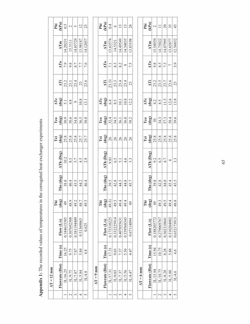
65

App

endi

x 1:

The

reco

rded

val

ues o

f tem

pera

ture

s in

the

corr

ugat

ed h

eat e

xcha

nger

exp

erim

ents

�

T =

12

mm

Fl

owra

te (H

ot)

Tim

e (s

) Fl

ow (L

/s)

Thi

(d

eg)

Tho

(deg

) �

Th

(Deg

) T

ci

(deg

) T

co

(deg

) �

Tc

(deg

) �

Ti

�T

o �

Tm

Ph

i (k

Pa)

1 3L

/16.

25

16.2

5 0.

1846

1538

5 49

38

.8

10.2

25

.8

30.9

5.

1 23

.2

7.9

14.2

0231

0.

5 2

3L/9

.75

9.75

0.

3076

9230

8 48

.9

40.4

8.

5 25

.8

30.6

4.

8 23

.1

9.8

15.5

111

2 3

3L/7

.87

7.87

0.

3811

9440

9 49

.2

43.5

5.

7 25

.8

34.8

9

23.4

8.

7 14

.857

29

5 4

3L/5

.84

5.84

0.

5136

9863

48

.7

44.2

4.

5 25

.7

36.5

10

.8

23

7.7

13.9

8187

12

5

3L/4

.8

4.8

0.62

5 49

.3

46.4

2.

9 25

.7

38.8

13

.1

23.6

7.

6 14

.120

57

25

�T

= 9

mm

Fl

owra

te (H

ot)

Tim

e (s

) Fl

ow (L

/s)

Thi

(d

eg)

Tho

(deg

) �

Th

(Deg

) T

ci

(deg

) T

co

(deg

) �

Tc

(deg

) �

Ti

�T

o �

Tm

Ph

i (k

Pa)

1 3L

/17.

31

17.3

1 0.

1733

1022

5 49

.31

39.5

9.

81

26

32.4

6.

4 23

.31

7.1

13.6

3574

0.

4 2

3L/9

.03

9.03

0.

3322

2591

4 49

.3

42.8

6.

5 26

34

.5

8.5

23.3

8.

3 14

.532

1 6

3 3L

/7.3

7 7.

37

0.40

7055

631

49.4

44

.3

5.1

26

36.1

10

.1

23.4

8.

2 14

.495

49

13

4 3L

/5.5

6 5.

56

0.53

9568

345

49.4

44

.8

4.6

26

36.8

10

.8

23.4

8

14.3

4835

15

5

3L/4

.47

4.47

0.

6711

4094

49

45

.7

3.3

26

38.2

12

.2

23

7.5

13.8

3198

28

�T

= 6

mm

Fl

owra

te (H

ot)

Tim

e (s

) Fl

ow (L

/s)

Thi

(d

eg)

Tho

(deg

) �

Th

(Deg

) T

ci

(deg

) T

co

(deg

) �

Tc

(deg

) �

Ti

�T

o �

Tm

Ph

i (k

Pa)

1 3L

/15.

94

15.9

4 0.

1882

0577

2 49

39

.8

9.2

25.8

30

4.

2 23

.2

9.8

15.5

4939

2

2 3L

/10.

75

10.7

5 0.

2790

6976

7 49

.3

42.8

6.

5 25

.8

34.3

8.

5 23

.5

8.5

14.7

5022

11

3

3L/8

.28

8.28

0.

3623

1884

1 49

.5

44.8

4.

7 25

.8

37.3

11

.5

23.7

7.

5 14

.079

95

20

4 3L

/5.8

8 5.

88

0.51

0204

082

49.4

45

.4

4 25

.8

38.4

12

.6

23.6

7

13.6

5877

35

5

3L/4

.6

4.6

0.65

2173

913

48.8

45

.5

3.3

25.8

39

.6

13.8

23

5.

9 12

.568

52

45

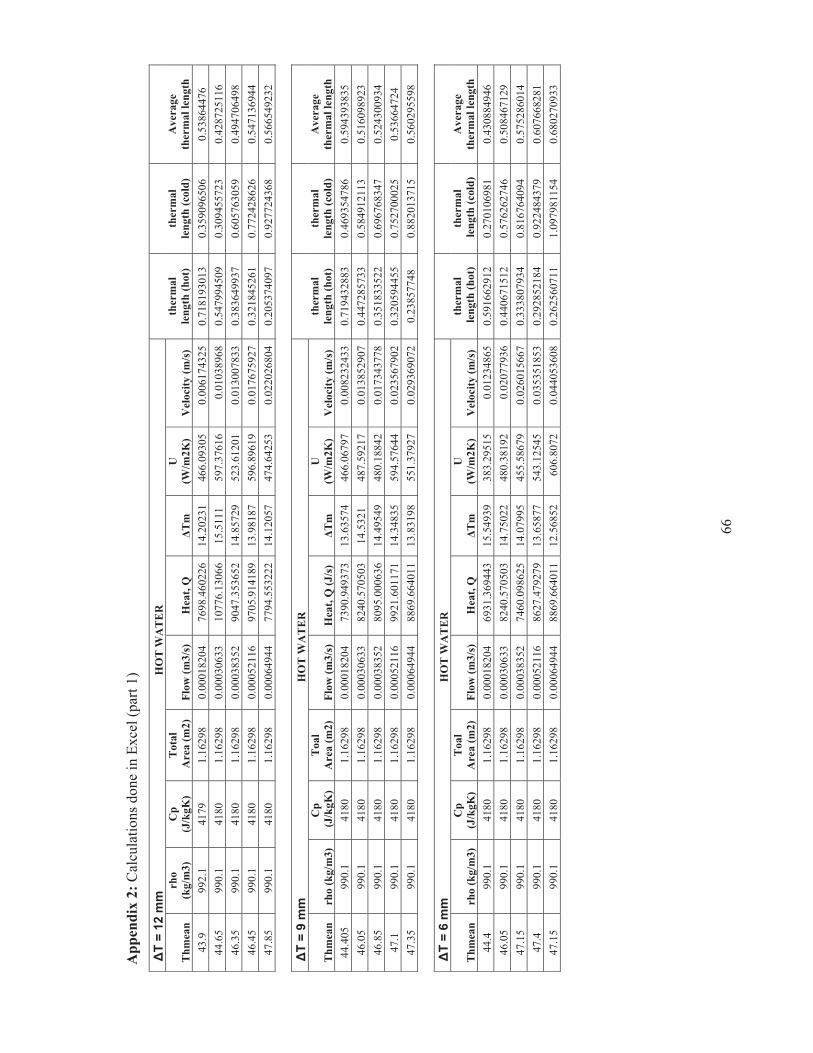
66

App

endi

x 2:

Cal

cula

tions

don

e in

Exc

el (p

art 1

)

�T

= 12

mm

HO

T W

AT

ER

Thm

ean

rho

(kg/

m3)

C

p

(J/k

gK)

Tot

al

Are

a (m

2)

Flow

(m3/

s)

Hea

t, Q

�T

m

U

(W/m

2K)

Vel

ocity

(m/s

) th

erm

al

leng

th (h

ot)

ther

mal

le

ngth

(col

d)

Ave

rage

th

erm

al le

ngth

43

.9

992.

1 41

79

1.16

298

0.00

0182

04

7698

.460

226

14.2

0231

46

6.09

305

0.00

6174

325

0.71

8193

013

0.35

9096

506

0.53

8644

76

44.6

5 99

0.1

4180

1.

1629

8 0.

0003

0633

10

776.

1306

6 15

.511

1 59

7.37

616

0.01

0389

68

0.54

7994

509

0.30

9455

723

0.42

8725

116

46.3

5 99

0.1

4180

1.

1629

8 0.

0003

8352

90

47.3

5365

2 14

.857

29

523.

6120

1 0.

0130

0783

3 0.

3836

4993

7 0.

6057

6305

9 0.

4947

0649

8 46

.45

990.

1 41

80

1.16

298

0.00

0521

16

9705

.914

189

13.9

8187

59

6.89

619

0.01

7675

927

0.32

1845

261

0.77

2428

626

0.54

7136

944

47.8

5 99

0.1

4180

1.

1629

8 0.

0006

4944

77

94.5

5322

2 14

.120

57

474.

6425

3 0.

0220

2680

4 0.

2053

7409

7 0.

9277

2436

8 0.

5665

4923

2

�

T =

9 m

m

H

OT

WA

TE

R

Thm

ean

rho

(kg/

m3)

C

p (J

/kgK

) T

oal

Are

a (m

2)

Flow

(m3/

s)

Hea

t, Q

(J/s

) �T

m

U

(W/m

2K)

Vel

ocity

(m/s

) th

erm

al

leng

th (h

ot)

ther

mal

le

ngth

(col

d)

Ave

rage

th

erm

al le

ngth

44

.405

99

0.1

4180

1.

1629

8 0.

0001

8204

73

90.9

4937

3 13

.635

74

466.

0679

7 0.

0082

3243

3 0.

7194

3288

3 0.

4693

5478

6 0.

5943

9383

5 46

.05

990.

1 41

80

1.16

298

0.00

0306

33

8240

.570

503

14.5

321

487.

5921

7 0.

0138

5290

7 0.

4472

8573

3 0.

5849

1211

3 0.

5160

9892

3 46

.85

990.

1 41

80

1.16

298

0.00

0383

52

8095

.000

636

14.4

9549

48

0.18

842

0.01

7343

778

0.35

1833

522

0.69

6768

347

0.52

4300

934

47.1

99

0.1

4180

1.

1629

8 0.

0005

2116

99

21.6

0117

1 14

.348

35

594.

5764

4 0.

0235

6790

2 0.

3205

9445

5 0.

7527

0002

5 0.

5366

4724

47

.35

990.

1 41

80

1.16

298

0.00

0649

44

8869

.664

011

13.8

3198

55

1.37

927

0.02

9369

072

0.23

8577

48

0.88

2013

715

0.56

0295

598

�T

= 6

mm

HO

T W

AT

ER

Thm

ean

rho

(kg/

m3)

C

p

(J/k

gK)

Toa

l A

rea

(m2)

Fl

ow (m

3/s)

H

eat,

Q

�Tm

U

(W

/m2K

) V

eloc

ity (m

/s)

ther

mal

le

ngth

(hot

) th

erm

al

leng

th (c

old)

A

vera

ge

ther

mal

leng

th

44.4

99

0.1

4180

1.

1629

8 0.

0001

8204

69

31.3

6944

3 15

.549

39

383.

2951

5 0.

0123

4865

0.

5916

6291

2 0.

2701

0698

1 0.

4308

8494

6 46

.05

990.

1 41

80

1.16

298

0.00

0306

33

8240

.570

503

14.7

5022

48

0.38

192

0.02

0779

36

0.44

0671

512

0.57

6262

746

0.50

8467

129

47.1

5 99

0.1

4180

1.

1629

8 0.

0003

8352

74

60.0

9862

5 14

.079

95

455.

5867

9 0.

0260

1566

7 0.

3338

0793

4 0.

8167

6409

4 0.

5752

8601

4 47

.4

990.

1 41

80

1.16

298

0.00

0521

16

8627

.479

279

13.6

5877

54

3.12

545

0.03

5351

853

0.29

2852

184

0.92

2484

379

0.60

7668

281

47.1

5 99

0.1

4180

1.

1629

8 0.

0006

4944

88

69.6

6401

1 12

.568

52

606.

8072

0.

0440

5360

8 0.

2625

6071

1 1.

0979

8115

4 0.

6802

7093

3

67

App

endi

x 3:

Cal

cula

tions

don

e in

Exc

el (p

art 2

)

�T

= 1

2 m

m

C

OL

D W

AT

ER

TC

mea

n rh

o (k

g/m

3)

Cp

(J/k

gK)

Toa

l Are

a (m

2)

Flow

(m3/

s)

Hea

t, Q

�T

m

Ave

rage

Hea

t U

(hot

_col

d)

(W/m

2.K

) 28

.35

996

4178

1.

1629

8 0.

0001

8204

4 38

63.4

3694

14

.202

3102

7 57

80.9

4858

3 34

9.99

9855

28

.2

996

4178

1.

1629

8 0.

0003

0632

9 61

18.6

7790

4 15

.511

1043

3 84

47.4

0428

1 46

8.28

2916

4 30

.3

996

4178

1.

1629

8 0.

0003

8352

3 14

363.

5454

3 14

.857

2942

2 11

705.

4495

4 67

7.44

8252

9 31

.1

996

4178

1.

1629

8 0.

0005

2115

7 23

421.

7920

5 13

.981

8743

6 16

563.

8531

2 10

18.6

4704

5 32

.25

996

4178

1.

1629

8 0.

0006

4943

8 35

402.

7465

8 14

.120

5733

6 21

598.

6499

13

15.2

3097

1

�T

= 9

mm

CO

LD

WA

TE

R

T

Cm

ean

rho

(kg/

m3)

C

p (J

/kgK

) T

oal A

rea

(m2)

Fl

ow (m

3/s)

H

eat,

Q

�Tm

A

vera

ge H

eat

U (h

ot_c

old)

(W

/m2.

K)

29.2

99

6 41

78

1.16

298

0.00

0182

044

4848

.234

591

13.6

3574

036

6119

.591

982

385.

8970

846

30.2

5 99

6 41

78

1.16

298

0.00

0306

329

1083

5.15

879

14.5

3209

776

9537

.864

645

564.

3526

882

31.0

5 99

6 41

78

1.16

298

0.00

0383

523

1611

9.08

987

14.4

9549

201

1210

7.04

525

718.

1794

246

31.4

99

6 41

78

1.16

298

0.00

0521

157

2342

1.79

205

14.3

4834

547

1667

1.69

661

999.

0925

661

32.1

99

6 41

78

1.16

298

0.00

0649

438

3297

0.49

681

13.8

3198

446

2092

0.08

041

1300

.488

784

�

T =

6 m

m

C

OL

D W

AT

ER

TC

mea

n rh

o (k

g/m

3)

Cp

(J/k

gK)

Toa

l Are

a (m

2)

Flow

(m3/

s)

Hea

t, Q

�T

m

Ave

rage

Hea

t U

(hot

_col

d)

(W/m

2.K

) 27

.9

996

4178

1.

1629

8 0.

0001

8204

4 31

81.6

5395

15

.549

3944

6 50

56.5

1169

7 27

9.61

8105

6 30

.05

996

4178

1.

1629

8 0.

0003

0632

9 10

835.

1587

9 14

.750

2160

4 95

37.8

6464

5 55

6.00

7343

4 31

.55

996

4178

1.

1629

8 0.

0003

8352

3 18

353.

4191

6 14

.079

9529

4 12

906.

7588

9 78

8.21

3280

3 32

.1

996

4178

1.

1629

8 0.

0005

2115

7 27

325.

4240

6 13

.658

7678

7 17

976.

4516

7 11

31.6

7103

7 32

.7

996

4178

1.

1629

8 0.

0006

4943

8 37

294.

4964

12

.568

5217

3 23

082.

0802

15

79.1

3223

6

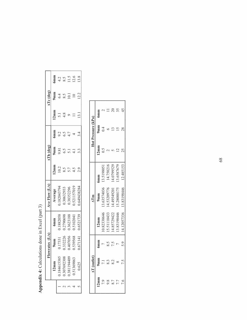
68

App

endi

x 4:

Cal

cula

tions

don

e in

Exc

el (p

art 3

)

Fl

owra

tes

(L/s

) A

ve F

low

(L/s

) �T

h (d

eg)

�Tc

(deg

)

12m

m

9mm

6m

m

Ave

rage

12

mm

9m

m

6mm

12

mm

9m

m

6mm

1

0.18

4615

385

0.17

331

0.18

8205

8 0.

1820

4379

4 10

.2

9.81

9.

2 5.

1 6.

4 4.

2 2

0.30

7692

308

0.33

2226

0.

2790

698

0.30

6329

33

8.5

6.5

6.5

4.8

8.5

8.5

3 0.

3811

9440

9 0.

4070

56

0.36

2318

8 0.

3835

2296

5.

7 5.

1 4.

7 9

10.1

11

.5

4 0.

5136

9863

0.

5395

68

0.51

0204

1 0.

5211

5701

9 4.

5 4.

1 4

11

10

12.6

5

0.62

5 0.

6711

41

0.65

2173

9 0.

6494

3828

4 2.

9 3.

3 3.

4 13

.1

12.2

13

.8

�T (o

utle

t)

�Tm

H

ot P

ress

ure

(kPa

) 12

mm

9m

m

6mm

12

mm

9m

m

6mm

12

mm

9m

m

6mm

7.

9 7.

1 7

10.8

2338

646

13.6

3574

036

13.5

1980

510.

5 0.

4 2

9.8

8.3

8.5

15.5

1110

433

14.5

3209

776

14.7

5021

62

6 11

8.

7 8.

2 7.

5 14

.857

2942

2 14

.495

4920

1 14

.079

9529

5 13

20

7.

7 8

7 13

.831

9844

6 15

.280

8817

5 13

.658

7679

12

15

35

7.6

7.5

5.9

14.1

2057

336

13.8

3198

446

12.4

8515

325

28

45

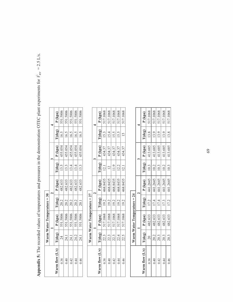
69

App

endi

x 5:

The

reco

rded

val

ues o

f tem

pera

ture

s and

pre

ssur

es in

the

dem

onst

ratio

n O

TEC

pla

nt e

xper

imen

ts fo

r W

FV�

= 2

.5 L

/s.

War

m W

ater

Tem

pera

ture

= 3

0 1

2 3

4 W

arm

flow

(L/s

) T

(deg

) P

(kpa

) T

(deg

) P

(kpa

) T

(deg

) P

(kpa

) T

(deg

) P

(kpa

) 0.

38

24

551.

5806

20

.2

482.

633

13.5

45

5.05

4 16

.5

551.

5806

0.

40

24.1

55

1.58

06

20.2

48

2.63

3 13

.3

455.

054

16.5

55

1.58

06

0.42

24

.1

551.

5806

20

.2

482.

633

13.4

45

5.05

4 16

.5

551.

5806

0.

44

24.2

55

1.58

06

20.2

48

2.63

3 13

.4

455.

054

16.5

55

1.58

06

0.46

24

.1

551.

5806

20

.1

482.

633

13.3

45

5.05

4 16

.5

551.

5806

War

m W

ater

Tem

pera

ture

= 2

7 1

2 3

4 W

arm

flow

(L/s

) T

(deg

) P

(kpa

) T

(deg

) P

(kpa

) T

(deg

) P

(kpa

) T

(deg

) P

(kpa

) 0.

38

22.3

51

7.10

68

19.2

46

8.84

35

12.1

43

4.37

15

.3

517.

1068

0.

40

22.3

51

7.10

68

19.2

46

8.84

35

12

434.

37

15.4

51

7.10

68

0.42

22

.3

517.

1068

19

.2

468.

8435

11

.9

434.

37

15.5

51

7.10

68

0.44

22

.4

517.

1068

19

.2

468.

8435

12

.2

434.

37

15.5

51

7.10

68

0.46

22

.5

517.

1068

19

.2

468.

8435

12

.1

434.

37

15

517.

1068

War

m W

ater

Tem

pera

ture

= 2

4 1

2 3

4 W

arm

flow

(L/s

) T

(deg

) P

(kpa

) T

(deg

) P

(kpa

) T

(deg

) P

(kpa

) T

(deg

) P

(kpa

) 0.

38

20

482.

633

17.2

44

1.26

45

10.3

41

3.68

5 13

.8

517.

1068

0.

40

20.2

48

2.63

3 17

.4

441.

2645

10

.2

413.

685

13.9

51

7.10

68

0.42

20

.3

482.

633

17.4

44

1.26

45

10.3

41

3.68

5 13

.9

517.

1068

0.

44

20.3

48

2.63

3 17

.3

441.

2645

10

.2

413.

685

13.9

51

7.10

68

0.46

20

.3

482.

633

17.2

44

1.26

45

10.3

41

3.68

5 13

.8

517.

1068

70

App

endi

x 6:

Cal

cula

tions

don

e in

EES

and

Exc

el (p

art 1

)

Tem

p Fl

ow (L

/s)

Vw

s/V

cs

P1

P2

P3

P1-P

2 P1

/P2

Twsi

-Tcs

i et

a (%

) 30

0.

38

2.41

55

1.58

06

482.

633

455.

054

68.9

476

1.14

2857

25

.5

1.03

6 30

0.

40

2.53

55

1.58

06

482.

633

455.

054

68.9

476

1.14

2857

25

.2

1.08

7 30

0.

42

2.59

55

1.58

06

482.

633

455.

054

68.9

476

1.14

2857

25

.3

1.09

5 30

0.

44

2.73

55

1.58

06

482.

633

455.

054

68.9

476

1.14

2857

25

.2

1.13

7 30

0.

46

2.86

55

1.58

06

482.

633

455.

054

68.9

476

1.14

2857

25

1.

147

Tem

p Fl

ow (L

/s)

Vw

s/V

cs

P1

P2

P3

P1-P

2 P1

/P2

Twsi

-Tcs

i et

a (%

) 27

0.

38

2.41

51

7.10

68

468.

8435

43

4.36

97

48.2

633

1.13

6364

22

.6

0.92

82

27

0.40

2.

53

517.

1068

46

8.84

35

434.

3697

48

.263

3 1.

1363

64

22.4

0.

9289

27

0.

42

2.59

51

7.10

68

468.

8435

42

7.47

5 48

.263

3 1.

1363

64

22.2

0.

9296

27

0.

44

2.73

51

7.10

68

468.

8435

43

4.36

97

48.2

633

1.10

2941

22

.6

0.97

93

27

0.46

2.

86

517.

1068

46

8.84

35

434.

3697

48

.263

3 1.

1029

41

22.5

1.

025

Tem

p Fl

ow (L

/s)

Vw

s/V

cs

P1

P2

P3

P1-P

2 P1

/P2

Twsi

-Tcs

i et

a (%

) 24

0.

38

2.41

48

2.63

3 44

1.26

45

406.

7907

41

.368

5 1.

0937

5 19

.7

0.84

37

24

0.40

2.

53

482.

633

441.

2645

41

3.68

54

41.3

685

1.09

375

19.8

0.

8448

24

0.

42

2.59

48

2.63

3 44

1.26

45

413.

6854

41

.368

5 1.

0937

5 19

.9

0.89

38

24

0.44

2.

73

482.

633

441.

2645

41

3.68

54

41.3

685

1.09

375

19.9

0.

9425

24

0.

46

2.86

48

2.63

3 44

1.26

45

413.

6854

41

.368

5 1.

0937

5 20

0.

9912

71

App

endi

x 7:

Cal

cula

tions

don

e in

EES

and

Exc

el (p

art 2

)

Tem

p rh

o1

rho2

rh

o3

rho4

T

1 T

sat1

Su

perh

eat

Tsa

t2

Tsa

t3

Tsa

t4

Wtu

r (W

) 30

26

.03

22.7

7 22

.09

1238

24

18

.83

5.17

14

.61

12.8

18

.83

6.14

667

30

26.0

2 22

.77

22.0

8 12

38

24.1

18

.83

5.27

14

.61

12.8

18

.83

6.44

998

30

26.0

2 22

.77

22.0

9 12

38

24.1

18

.83

5.27

14

.61

12.8

18

.83

6.44

998

30

26

22.7

7 22

.08

1238

24

.2

18.8

3 5.

37

14.6

1 12

.8

18.8

3 6.

7501

95

30

26.0

2 22

.79

22.1

12

38

24.1

18

.83

5.27

14

.61

12.8

19

.22

6.64

806

Tem

p rh

o1

rho2

rh

o3

rho4

T

1 T

sat1

Su

perh

eat

Tsa

t2

Tsa

t3

Tsa

t4

Wtu

r (W

) 27

24

.38

22.1

5 21

.09

1242

22

.3

16.7

7 5.

53

13.7

1 11

.38

16.7

7 5.

5486

35

27

24.3

8 22

.15

21.1

12

42

22.3

16

.77

5.53

13

.71

11.3

8 16

.77

5.54

8635

27

24

.38

22.1

5 21

.11

1242

22

.3

16.7

7 5.

53

13.7

1 11

.38

16.7

7 5.

5486

35

27

24.3

7 22

.15

21.0

8 12

42

22.4

16

.77

5.63

16

.77

13.7

1 11

.38

5.84

6715

27

24

.35

22.1

5 21

.09

1244

22

.5

16.7

7 5.

73

13.7

1 11

.38

16.7

7 6.

1578

T

emp

rho1

rh

o2

rho3

rh

o4

T1

Tsa

t1

Supe

rhea

t T

sat2

T

sat3

T

sat4

W

tur

(W)

24

22.8

20

.89

20.1

4 12

48

20

14.6

1 5.

39

11.8

6 9.

913

16.7

7 5.

0856

24

22

.77

20.8

7 20

.15

1248

20

.2

14.6

1 5.

59

11.8

6 9.

913

16.7

7 5.

0949

6 24

22

.76

20.8

7 20

.14

1248

20

.3

14.6

1 5.

69

11.8

6 9.

913

16.7

7 5.

3913

6 24

22

.76

20.8

8 20

.15

1248

20

.3

14.6

1 5.

69

11.8

6 9.

913

16.7

7 5.

6846

4 24

22

.76

20.8

9 20

.15

1248

20

.3

14.6

1 5.

69

11.8

6 9.

913

16.7

7 5.

9810

4

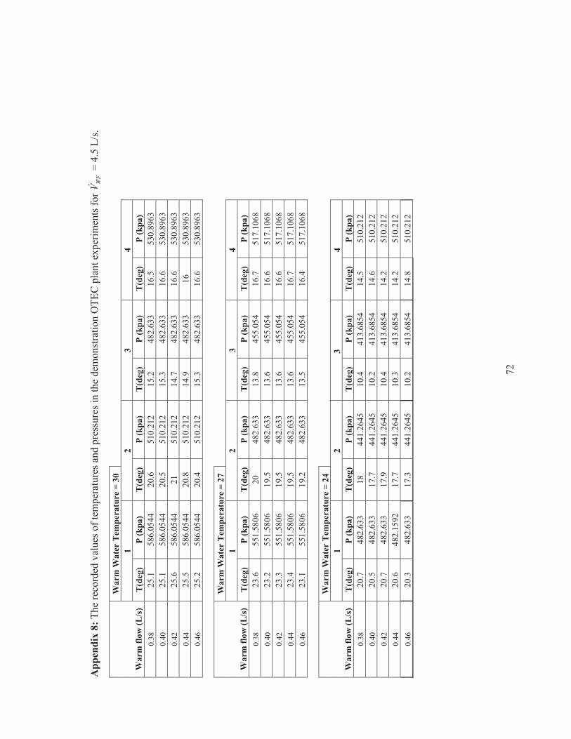
72

App

endi

x 8:

The

reco

rded

val

ues o

f tem

pera

ture

s and

pre

ssur

es in

the

dem

onst

ratio

n O

TEC

pla

nt e

xper

imen

ts fo

r W

FV�

= 4

.5 L

/s.

War

m W

ater

Tem

pera

ture

= 3

0 1

2 3

4 W

arm

flow

(L/s

) T

(deg

) P

(kpa

) T

(deg

) P

(kpa

) T

(deg

) P

(kpa

) T

(deg

) P

(kpa

) 0.

38

25.1

58

6.05

44

20.6

51

0.21

2 15

.2

482.

633

16.5

53

0.89

63

0.40

25

.1

586.

0544

20

.5

510.

212

15.3

48

2.63

3 16

.6

530.

8963

0.

42

25.6

58

6.05

44

21

510.

212

14.7

48

2.63

3 16

.6

530.

8963

0.

44

25.5

58

6.05

44

20.8

51

0.21

2 14

.9

482.

633

16

530.

8963

0.

46

25.2

58

6.05

44

20.4

51

0.21

2 15

.3

482.

633

16.6

53

0.89

63

W

arm

Wat

er T

empe

ratu

re =

27

1 2

3 4

War

m fl

ow (L

/s)

T(d

eg)

P (k

pa)

T(d

eg)

P (k

pa)

T(d

eg)

P (k

pa)

T(d

eg)

P (k

pa)

0.38

23

.6

551.

5806

20

48

2.63

3 13

.8

455.

054

16.7

51

7.10

68

0.40

23

.2

551.

5806

19

.5

482.

633

13.6

45

5.05

4 16

.6

517.

1068

0.

42

23.3

55

1.58

06

19.5

48

2.63

3 13

.6

455.

054

16.6

51

7.10

68

0.44

23

.4

551.

5806

19

.5

482.

633

13.6

45

5.05

4 16

.7

517.

1068

0.

46

23.1

55

1.58

06

19.2

48

2.63

3 13

.5

455.

054

16.4

51

7.10

68

W

arm

Wat

er T

empe

ratu

re =

24

1 2

3

4 W

arm

flow

(L/s

) T

(deg

) P

(kpa

) T

(deg

) P

(kpa

) T

(deg

) P

(kpa

) T

(deg

) P

(kpa

) 0.

38

20.7

48

2.63

3 18

44

1.26

45

10.4

41

3.68

54

14.5

51

0.21

2 0.

40

20.5

48

2.63

3 17

.7

441.

2645

10

.2

413.

6854

14

.6

510.

212

0.42

20

.7

482.

633

17.9

44

1.26

45

10.4

41

3.68

54

14.2

51

0.21

2 0.

44

20.6

48

2.15

92

17.7

44

1.26

45

10.3

41

3.68

54

14.2

51

0.21

2 0.

46

20.3

48

2.63

3 17

.3

441.

2645

10

.2

413.

6854

14

.8

510.

212

73

App

endi

x 9:

Cal

cula

tions

don

e in

EES

and

Exc

el (p

art 1

)

Tem

p Fl

ow(L

/s)

Vw

s/V

cs

P1

P2

P3

P1-P

2 P1

/P2

Twsi

-Tcs

i et

a (%

) 30

0.

38

2.41

58

6.05

44

510.

212

482.

633

75.8

4233

1.

1486

49

25.6

1.

316

30

0.40

2.

53

586.

0544

51

0.21

2 46

1.94

87

75.8

4233

1.

0810

81

25.6

1.

367

30

0.42

2.

59

586.

0544

51

0.21

2 46

1.94

87

75.8

4233

1.

0810

81

25.5

1.

37

30

0.44

2.

73

586.

0544

51

0.21

2 48

2.63

3 75

.842

33

1.08

1081

25

.6

1.41

3 30

0.

46

2.86

58

6.05

44

510.

212

475.

7383

75

.842

33

1.14

8649

25

.4

1.46

8

T

emp

Flow

(L/s

) V

ws/

Vcs

P1

P2

P3

P1

-P2

P1/P

2 Tw

si-T

csi

eta

(%)

27

0.38

2.

41

551.

5806

48

2.63

3 45

5.05

4 68

.947

57

1.12

6761

22

.7

0.93

52

27

0.40

2.

53

551.

5806

48

2.63

3 45

5.05

4 68

.947

57

1.14

2857

22

.4

0.98

18

27

0.42

2.

59

551.

5806

48

2.63

3 45

5.05

4 68

.947

57

1.14

2857

22

.3

1.03

3 27

0.

44

2.73

55

1.58

06

482.

633

455.

054

68.9

4757

1.

1267

61

22.6

1.

084

27

0.46

2.

86

551.

5806

48

2.63

3 45

5.05

4 68

.947

57

1.14

2857

22

.2

1.13

2

T

emp

Flow

(L/s

) V

ws/

Vcs

P1

P2

P3

P1

-P2

P1/P

2 Tw

si-T

csi

eta

(%)

24

0.38

2.

41

482.

633

441.

2645

41

3.68

54

41.3

6854

1.

0937

5 19

.6

0.80

09

24

0.40

2.

53

482.

633

441.

2645

41

3.68

54

41.3

6854

1.

0937

5 19

.8

0.84

98

24

0.42

2.

59

482.

633

441.

2645

41

3.68

54

41.3

6854

1.

0937

5 19

.6

0.84

79

24

0.44

2.

73

482.

633

441.

2645

41

3.68

54

41.3

6854

1.

0926

76

19.8

0.

8963

24

0.

46

2.86

48

2.63

3 44

1.26

45

413.

6854

41

.368

54

1.09

375

19.8

0.

9486

74

App

endi

x 10

: Cal

cula

tions

don

e in

EES

and

Exc

el (p

art 2

)

Tem

p rh

o1

rho2

rh

o3

rho4

T

1 T

sat1

Su

perh

eat

Tsa

t2

Tsa

t3

Tsa

t4

Wtu

r (W

) 30

27

.77

24.2

3 23

.41

1238

25

.1

20.7

8 4.

32

16.3

5 14

.61

17.6

1 14

.066

78

30

27.7

7 24

.24

23.3

9 12

38

25.1

20

.78

4.32

16

.35

14.6

1 17

.61

14.6

0159

30

27

.7

24.1

7 23

.47

1238

25

.6

20.7

8 4.

82

16.3

5 14

.61

17.6

1 14

.668

44

30

27.7

1 24

.2

23.4

5 12

40

25.5

20

.78

4.72

16

.35

14.6

1 17

.61

15.2

1666

30

27

.76

24.2

5 23

.39

1238

25

.2

20.7

8 4.

42

16.3

5 14

.61

17.6

1 15

.693

51

Tem

p rh

o1

rho2

rh

o3

rho4

T

1 T

sat1

Su

perh

eat

Tsa

t2

Tsa

t3

Tsa

t4

Wtu

r (W

) 27

26

.09

22.8

22

.04

1237

23

.6

18.8

3 4.

77

14.6

1 12

.8

16.7

7 9.

9417

69

27

26.1

5 22

.86

22.0

4 12

38

23.2

18

.83

4.37

14

.61

12.8

16

.77

10.4

2891

27

26

.13

22.8

6 22

.06

1238

23

.3

18.8

3 4.

47

14.6

1 12

.8

16.7

7 10

.974

87

27

26.1

2 22

.86

22.0

6 12

37

23.4

18

.83

4.57

14

.61

12.8

16

.77

11.5

1152

27

26

.15

22.9

22

.08

1238

23

.1

18.8

3 4.

27

14.6

1 12

.8

16.7

7 12

.033

36

Tem

p rh

o1

rho2

rh

o3

rho4

T

1 T

sat1

Su

perh

eat

Tsa

t2

Tsa

t3

Tsa

t4

Wtu

r (W

) 24

22

.71

20.8

20

.13

1245

20

.7

14.6

1 6.

09

11.8

6 9.

913

16.3

5 8.

6558

63

24

22.7

4 20

.84

20.1

5 12

45

20.5

14

.61

5.89

11

.86

9.91

3 16

.35

9.17

1293

24

22

.71

20.8

1 20

.13

1246

20

.7

14.6

1 6.

09

11.8

6 9.

913

16.3

5 9.

1898

73

24

22.7

3 20

.84

20.1

4 12

46

20.6

14

.61

5.99

11

.86

9.91

3 16

.35

9.71

1324

24

22

.76

20.8

8 20

.15

1244

20

.3

14.6

1 5.

69

11.8

6 9.

913

16.3

5 10

.199

56