Design and Verification ofSituation-aware Real-time Systems

by

Nayreet Islam

A thesis submitted to theSchool of Graduate and Postdoctoral Studies in partial

fulfillment of the requirements for the degree of

Master of Applied Science in Electrical and Computer Engineering

Faculty of Engineering and Applied ScienceUniversity of Ontario Institute of Technology

Oshawa, Ontario, Canada

December 2018

©Nayreet Islam, 2018

THESIS EXAMINATION INFORMATION

Submitted by: Nayreet Islam

Masters of Applied Science in Electrical and Computer Engineering

Thesis title: Design and Verification of Situation-Aware Real-Time Systems

An oral defense of this thesis took place on December 12, 2018 in front of the following examining

committee:

Examining Committee:

Chair of Examining Committee

Dr. Walid Morsi Ibrahim

Research Supervisor

Dr. Akramul Azim

Examining Committee Member

Dr. Qusay Mahmoud

External Examiner

Dr. Jing Ren, UOIT - FEAS

The above committee determined that the thesis is acceptable in form and content and that a

satisfactory knowledge of the field covered by the thesis was demonstrated by the candidate during

an oral examination. A signed copy of the Certificate of Approval is available from the School of

Graduate and Postdoctoral Studies.

ABSTRACT

A real-time system (RTS) is usually well-defined and operates based on a specific model

defined during system design. However, the RTS can interact with different objects from

its environment and needs to satisfy a number of user-defined constraints such as safety

(defined using the probability of failure) and performance (defined using the percentage

of usage). Such requirements create the necessity for the RTS to be aware of its design

and execute a set of additional tasks (apart from the tasks whose order is defined by a

particular scheduler during system design) in response to the events which take place in

the environment.

This thesis presents the design of a situation-aware RTS which can characterize the

environmental situations through monitoring the system environment, analyzing the

input obtained from the environment and identifying real-world occurrences as events.

Additionally, we determine the real-time and non real-time properties associated with

the events, identify the relationships involved among the events and create a knowledge-

base offline which facilitates a reduced size of data for storage and processing.

We present a situation-aware task model (SATM) which efficiently maps the identi-

fied environmental events to a set of (predefined) adaptive tasks offline. This thesis

also presents a validation framework which determines the user-defined safety, and per-

formance constraints. We consider that the situation-aware RTS has two modes of

operation: safety, and performance. The validation framework performs an online iden-

tification of the expected mode based on the user-defined constraints, checks whether the

RTS is operating in the correct mode or not and allows the RTS to change its operating

mode (if necessary).

To demonstrate the applicability of the proposed situation-aware RTS and usability of

the SATM, the experimental analysis of the thesis is performed using three case studies:

an automotive system, a real-time traffic monitoring system and an unmanned aerial

vehicle (UAV) system which include RTS that are in motion and static. For the auto-

motive system case-study, the experimental results of this thesis show that we identify

17234 events in 3241 environmental situations. The system operates in performance

mode in 3295 situations and in safety mode in 126 situations when the probability of

failure is high. The system consists of five tasks in the performance mode and three

tasks in the safety mode and the corresponding constructed SATM contains nine ver-

tices (adaptive tasks) and 68 edges. For each case-study, the constructed SATM provides

an improvement in terms of scheduling overhead (up to 21%) and adaptation time (up

to 49%) with respect to existing task models task models such as generalized multiframe

model (GMF), non-cyclic generalized multiframe model (NC-GMF), recurring branch-

ing (RB), recurring real-time task (RRT), and non-cyclic recurring real-time task model

(NC-RRT).

AUTHORS DECLARATION

I hereby declare that this thesis consists of original work of which I have authored. This

is a true copy of the thesis, including any required final revisions, as accepted by my

examiners.

I authorize the University of Ontario Institute of Technology to lend this thesis to other

institutions or individuals for the purpose of scholarly research. I further authorize

University of Ontario Institute of Technology to reproduce this thesis by photocopying

or by other means, in total or in part, at the request of other institutions or individuals for

the purpose of scholarly research. I understand that my thesis will be made electronically

available to the public.

Nayreet Islam

ii

STATEMENT OF CONTRIBUTIONS

The contributions of the thesis are listed as follows:

Contribution 1: In Chapter 3, we present the design of a situation-aware real-time

system which identifies real-time occurrences from the system environment as events,

determines their properties, identifies the relationships among the events, characterizes

the environmental situations in terms of events and creates a knowledge-base which

allows faster information retrieval in a reduced memory space (in comparison to raw

input data).

Contribution 2: In Chapter 4, we form a situation-aware graph-based task model by

identifying the adaptive tasks needed to be executed in response to the current situations

based on the detected events, evaluating the adaptive task defining a number of timing

constraints and including the tasks in the proposed task model if the constraints are

met.

Contribution 3: In Chapter 5, we present a validation framework that uses the

knowledge-base to analyze the user-defined (safety and performance) constraints of the

situation-aware real-time system, identifies the expected mode, determines whether the

system is operating in the expected mode or not, and triggers a verification action (if

necessary) which allows the system to switch the mode.

Parts of Contribution 1 and Contribution 3 presented in Chapter 3 and Chapter 5 have

already been published as:

• Islam, Nayreet, and Akramul Azim. ”A multi-mode real-time system verification

model using efficient event-driven dataset.” Journal of Ambient Intelligence and

Humanized Computing, pages: 1-14, 2018.

• Islam, Nayreet, and Akramul Azim. ”CARTS: Constraint-based analytics from

real-time system monitoring.” Proceedings of the IEEE International Conference

on Systems, Man, and Cybernetics (SMC), pp: 2164-2169, 2017, Canada.

• Islam, Nayreet, and Akramul Azim. ”Assuring the runtime behavior of self-

adaptive cyber-physical systems using feature modeling.” Proceedings of the 28th

Annual International Conference on Computer Science and Software Engineering

(CASCON), pp: 48-59, 2018, Canada.

iii

ACKNOWLEDGEMENTS

I would like to express my heartiest gratitude to the Almighty for the strength he

provided me to finalize this thesis.

I want to express the most profound appreciation to my supervisor Dr. Akramul Azim

for his invaluable guidance, support and immense inspiration towards the completion of

this thesis. You always provided me the best directions, advice, and novel ideas. Thanks

for giving me the freedom and flexibility to explore interesting research problems in real-

time system domain. Thanks for believing in me and helping me in finishing this thesis.

Without your extreme patience, knowledge, and encouragement my MASc study would

not be achievable.

A sincere appreciation to my colleagues at RTEMSOFT research group (especially Md

Al Maruf and Mellitus Ezeme) who have always helped me with helpful criticism during

my MASc work. Many thanks go to the members of the Software System Research Lab

who contributed to the friendly atmosphere in my workplace. I also thank all my friends,

colleagues and my fiance Afsana Alam who always cheered me up, provided courage and

mental support as well as motivated me through this journey.

I am thankful to my family, especially my beloved mother Shelina Begum, my father

Rafiqul Islam, my sister Ananaya Islam, and my late grandmother Dolena Begum for

their unconditional support and love. Belonging to a social setting where typically most

young people voluntarily or involuntarily rest their case to education at an early age,

my parents pushed me to seek admission in a top ranking university in Bangladesh, and

eventually pursue a MASc degree in UOIT. My parents are my heroes who have worked

very hard so that my sister and I can achieve our personal and career goal. I appreciate

and thank my parents for understanding and believing in me. Without you, I could not

make this valuable journey happen.

iv

Contents

Abstract i

AUTHORS DECLARATION ii

Acknowledgements iv

List of Figures viii

List of Tables ix

Abbreviations x

1 Introduction 1

1.1 Design aspects of real-time systems . . . . . . . . . . . . . . . . . . . . . . 1

1.1.1 Timeliness . . . . . . . . . . . . . . . . . . . . . . . . . . . . . . . . 2

1.1.2 Schedulability . . . . . . . . . . . . . . . . . . . . . . . . . . . . . . 2

1.1.3 Multi-mode operation . . . . . . . . . . . . . . . . . . . . . . . . . 3

1.2 Challenges with the state-of-the-art in real-time systems . . . . . . . . . . 3

1.3 Thesis objectives . . . . . . . . . . . . . . . . . . . . . . . . . . . . . . . . 4

1.4 Design and verification of situation-aware real-time systems . . . . . . . . 5

1.5 Contributions . . . . . . . . . . . . . . . . . . . . . . . . . . . . . . . . . . 6

1.6 Novelty of the thesis . . . . . . . . . . . . . . . . . . . . . . . . . . . . . . 8

1.7 Organization of the thesis . . . . . . . . . . . . . . . . . . . . . . . . . . . 8

2 Literature review 10

2.1 Introduction . . . . . . . . . . . . . . . . . . . . . . . . . . . . . . . . . . . 10

2.2 Fundamentals . . . . . . . . . . . . . . . . . . . . . . . . . . . . . . . . . . 10

2.2.1 Real-time system task model . . . . . . . . . . . . . . . . . . . . . 10

2.2.1.1 Internal task set . . . . . . . . . . . . . . . . . . . . . . . 11

2.2.1.2 Adaptive task set . . . . . . . . . . . . . . . . . . . . . . 12

2.3 Related works . . . . . . . . . . . . . . . . . . . . . . . . . . . . . . . . . . 13

2.3.1 Real-time task model . . . . . . . . . . . . . . . . . . . . . . . . . 13

2.3.2 Situation characterization . . . . . . . . . . . . . . . . . . . . . . . 14

2.3.3 Validation of real-time systems . . . . . . . . . . . . . . . . . . . . 15

2.3.3.1 Safety analysis . . . . . . . . . . . . . . . . . . . . . . . . 15

v

Contents vi

2.3.4 Self-adaptation . . . . . . . . . . . . . . . . . . . . . . . . . . . . . 16

3 Components of the proposed situation-aware real-time system 18

3.1 Introduction . . . . . . . . . . . . . . . . . . . . . . . . . . . . . . . . . . . 18

3.2 Operational environment model . . . . . . . . . . . . . . . . . . . . . . . . 18

3.2.1 Data capture module . . . . . . . . . . . . . . . . . . . . . . . . . . 19

3.2.2 Detection module . . . . . . . . . . . . . . . . . . . . . . . . . . . . 19

3.2.2.1 Object identifier . . . . . . . . . . . . . . . . . . . . . . . 20

3.2.2.2 Object classifier . . . . . . . . . . . . . . . . . . . . . . . 21

3.2.2.3 Object tracker . . . . . . . . . . . . . . . . . . . . . . . . 21

3.2.2.4 Event identifier . . . . . . . . . . . . . . . . . . . . . . . . 22

3.2.3 Analytics module . . . . . . . . . . . . . . . . . . . . . . . . . . . . 23

3.2.3.1 Event properties extractor . . . . . . . . . . . . . . . . . 23

3.2.3.2 Event classifier . . . . . . . . . . . . . . . . . . . . . . . . 24

3.2.3.3 Characterization of situations . . . . . . . . . . . . . . . . 24

4 Mapping situations to tasks in the situation-aware real-time system 25

4.1 Introduction . . . . . . . . . . . . . . . . . . . . . . . . . . . . . . . . . . . 25

4.2 Workflow of the situation-aware real-time system . . . . . . . . . . . . . . 25

4.2.1 Monitoring the environment of the real-time system . . . . . . . . 26

4.2.2 Characterizing environmental situation . . . . . . . . . . . . . . . . 26

4.2.2.1 Identifying objects and events . . . . . . . . . . . . . . . 26

4.2.2.2 Analyzing the properties of the events . . . . . . . . . . . 27

4.2.2.3 Identifying the relationships involved among events . . . 29

4.2.3 Creating the knowledge-base . . . . . . . . . . . . . . . . . . . . . 30

4.2.4 Satisfying the user-defined constraints . . . . . . . . . . . . . . . . 31

4.2.5 Identifying adaptive tasks in a particular situation . . . . . . . . . 32

4.2.6 Execution model of the proposed situation-aware real-time system 33

4.2.7 Using existing task models to execute adaptive tasks . . . . . . . . 34

4.3 Proposed situation-aware graph-based task model . . . . . . . . . . . . . . 35

4.3.1 Characterizing adaptive tasks using SATM . . . . . . . . . . . . . 35

4.3.2 Evaluating timing constraints . . . . . . . . . . . . . . . . . . . . . 35

4.3.3 Evaluating graph-based properties . . . . . . . . . . . . . . . . . . 36

4.3.4 Identifying the execution order of adaptive tasks . . . . . . . . . . 38

4.3.5 Schedulibility analysis of adaptive tasks for each situation . . . . . 41

4.4 Discussion . . . . . . . . . . . . . . . . . . . . . . . . . . . . . . . . . . . . 43

5 Analyzing user-defined constraints for the situation-aware real-timesystem 44

5.1 Introduction . . . . . . . . . . . . . . . . . . . . . . . . . . . . . . . . . . . 44

5.2 Identifying the safety constraint . . . . . . . . . . . . . . . . . . . . . . . . 45

5.3 Identifying the performance constraint . . . . . . . . . . . . . . . . . . . . 47

5.4 Identifying the expected mode . . . . . . . . . . . . . . . . . . . . . . . . . 48

5.5 Satisfying the user-defined constraints . . . . . . . . . . . . . . . . . . . . 49

5.5.1 Predictive analysis . . . . . . . . . . . . . . . . . . . . . . . . . . . 50

5.5.1.1 Motion modeling using LSTM . . . . . . . . . . . . . . . 50

5.6 Discussion . . . . . . . . . . . . . . . . . . . . . . . . . . . . . . . . . . . . 52

Contents vii

6 Experimental analysis 53

6.1 Introduction . . . . . . . . . . . . . . . . . . . . . . . . . . . . . . . . . . . 53

6.2 Objectives of the experimental analysis . . . . . . . . . . . . . . . . . . . . 53

6.3 Experimental case studies . . . . . . . . . . . . . . . . . . . . . . . . . . . 54

6.4 Operational environment model . . . . . . . . . . . . . . . . . . . . . . . . 55

6.4.1 Real-time object identification and detection . . . . . . . . . . . . 55

6.4.2 Identification of events along with their real-time and non-realtime properties . . . . . . . . . . . . . . . . . . . . . . . . . . . . . 56

6.4.3 Formation of a knowledge-base . . . . . . . . . . . . . . . . . . . . 57

6.5 The proposed situation-aware graph-based task model . . . . . . . . . . . 57

6.5.1 Comparative analysis of the resource demands of the adaptivetasks in different case studies . . . . . . . . . . . . . . . . . . . . . 57

6.5.2 Evaluation of timing constraint and graph-based properties . . . . 59

6.5.2.1 Comparison of scheduling overhead with vs. withouttiming evaluation . . . . . . . . . . . . . . . . . . . . . . 59

6.5.2.2 Comparison of the probability of failure with vs. withouttiming evaluation . . . . . . . . . . . . . . . . . . . . . . 61

6.5.2.3 Comparison of self-adaptation time with vs. withouttiming evaluation . . . . . . . . . . . . . . . . . . . . . . 61

6.5.3 Comparative analysis of SATM with existing task models . . . . . 61

6.5.4 Characteristics of generated SATM . . . . . . . . . . . . . . . . . . 64

6.5.5 Comparative analysis of the adaptation time (SATM vs. existingtask models) . . . . . . . . . . . . . . . . . . . . . . . . . . . . . . 66

6.6 Satisfying user-defined constraints . . . . . . . . . . . . . . . . . . . . . . 68

6.6.1 Identifying the safety constraint . . . . . . . . . . . . . . . . . . . 68

6.6.2 Identifying the performance constraint . . . . . . . . . . . . . . . . 68

6.6.3 Validation framework . . . . . . . . . . . . . . . . . . . . . . . . . 71

6.6.3.1 Comparative analysis of modes changes (with vs. with-out validation framework) . . . . . . . . . . . . . . . . . . 71

6.6.4 Predictive analysis . . . . . . . . . . . . . . . . . . . . . . . . . . . 74

7 Conclusion 76

A An Appendix 79

Bibliography 81

List of Figures

1.1 Design and verification of the situation-aware real-time system . . . . . . 5

3.1 Components of operational environment model of the situation-awarereal-time system. . . . . . . . . . . . . . . . . . . . . . . . . . . . . . . . . 20

4.1 Identification and analysis of the properties of events . . . . . . . . . . . . 28

4.2 Execution model of the situation-aware RTS . . . . . . . . . . . . . . . . . 34

5.1 Our approach for RTS failure analysis using fault tree . . . . . . . . . . . 45

5.2 Workflow for generating expected behavior of the system using validationframework . . . . . . . . . . . . . . . . . . . . . . . . . . . . . . . . . . . . 46

5.3 Validation framework . . . . . . . . . . . . . . . . . . . . . . . . . . . . . 48

5.4 Mode switching in RTS . . . . . . . . . . . . . . . . . . . . . . . . . . . . 49

6.1 Real-time object identification and classification using our approach . . . 56

6.2 Comparative analysis of resource demands in different case studies . . . . 58

6.3 Comparative analysis of the scheduling overload using vs. without usingtiming evaluations . . . . . . . . . . . . . . . . . . . . . . . . . . . . . . . 60

6.4 A comparison of probability of failure (with vs without evaluation) . . . . 62

6.5 Improvement of adaptation timing and graph-based evaluation. . . . . . . 63

6.6 Performance comparison of different task models with SATM . . . . . . . 65

6.7 Improvement of adaptation time due to SATM at runtime. . . . . . . . . 67

6.8 Probability of failure of the situation-aware RTS in different timestampsfor Case-study 1 . . . . . . . . . . . . . . . . . . . . . . . . . . . . . . . . 69

6.9 Percentage of usage due to detecting and processing events . . . . . . . . 70

6.10 Changes of modes of operation in different time interval . . . . . . . . . . 72

6.11 A comparison of mode changes with vs. without validation framework . . 73

6.12 Prediction of collision using Motion modeling . . . . . . . . . . . . . . . . 74

viii

List of Tables

2.1 An example list of internal task set in Safety and Performance mode. . . 11

6.1 Statistics of the detected events. . . . . . . . . . . . . . . . . . . . . . . . 57

6.2 List of adaptive tasks considered in this work in different case studies . . 59

6.3 Characteristics of the SATM. . . . . . . . . . . . . . . . . . . . . . . . . . 66

ix

Abbreviations

RTS Real-time system

OEM Operational environment model

SATM Situation-aware graph-based task model

UAV Unmanned aerial vehicle

CNN Convolutional Neural Network

RNN Recurrent neural network

LSTM Long short-term memory

GMF Generalized Multiframe Model

NC - GMF Non-cyclic Generalized Multiframe Model

RB Recurring Branching Task Model

RRT Recurring Real-time Task Model

NC - RRT Non-cyclic Recurring Real-time Task Model

EDF Earliest Deadline First

TINA Time Petri Net Analysis

YOLO You Only Look Once

SIL Safety Integrity Level

TC Timing Constraints

GC Graph-based Constraints

x

Chapter 1

Introduction

Real-time systems are those computing systems which need to react within a precise time

in response to an event taking place inside the system or in the environment [1]. Such

systems often include a number of concurrent tasks sharing the execution processors [2].

A task can be defined as the real-time computation that is executed by the processor in

a sequential fashion [1]. Real-time computations are extensively integrated (in part or

completely) to a number of application domains such as Automotive, Avionics, Railway,

Telecommunication, Robotics and Military [1].

Correct behavior of an RTS depends not only on the value of the computation associated

with the task but also the time at which the task has finished its execution. For example:

upon the detection of a collision, an automotive real-time system needs to execute the

task which activates the airbag. Late activation of the airbag may result in driver

hitting the steering wheel. Hence a missed deadline of any real-time task can result in

catastrophic consequence or may lead to significant loss. Therefore, the RTS must be

designed carefully so that the system can guarantee meeting the deadlines of the tasks.

1.1 Design aspects of real-time systems

Several design aspects exist that must be carefully defined and reviewed by the RTS

designers which include timeliness, schedulability, and multi-mode operation. These

aspects make the design of an RTS challenging. The real-time system can achieve

predictability by satisfying the design aspects described as follows:

1

Chapter 1 2

1.1.1 Timeliness

Tasks with strict timing constraints characterize an RTS. The timing constraints associ-

ated with the tasks need to be satisfied in order to accomplish the expected behavior [1].

One of the common timing constraints of the real-time task is its deadline. The deadline

of a task represents the time before which it must complete its execution [1].

For example, an automotive RTS can contain a task for fuel injection whose relative

deadline is 40 milliseconds which means it must complete its execution within next 40

milliseconds with respect to the arrival time of the task. The designer of the RTS

specifies the tasks to be handled by the system and the general timing requirements

associated with the tasks that the system must satisfy.

1.1.2 Schedulability

An RTS may need to execute several tasks which can overlap in time. The processor of

the RTS needs to be assigned to the various tasks based on a certain predefined criterion

called a scheduling policy. The RTS can interrupt the running task so that important

tasks can gain the processor immediately upon arrival. The operation of suspending a

running task is called preemption. A scheduling algorithm can be defined as a set of rules

that, at any time, determines the order in which tasks are executed [1]. A schedule of a

set of tasks is said to be feasible if all the tasks can complete their execution according

to a set of predefined constraints [1]. A set of tasks is said to be schedulable if there

exists at least one algorithm that can produce a feasible schedule. The RTS must be

able to determine the schedulability.

A number of techniques have been proposed in the literature for scheduling the real-

time tasks. If the task executions can be interrupted, the scheduling policy is called

preemptive scheduling [3]. Otherwise, the policy is called non-preemptive scheduling [4].

Static cyclic scheduling implies the off-line generation of a fixed schedule table that

will be followed at runtime to order task executions [5, 6]. Priority based scheduling

policies select and execute the task with the highest priority when there are requests from

multiple tasks. Depending on whether the priority of a task is constant or not, priority-

based scheduling can be further divided into two groups, static priority scheduling and

dynamic priority scheduling [1, 7].

Chapter 1 3

1.1.3 Multi-mode operation

An RTS today is often expected to operate in multiple modes. Each operating mode

corresponds to specific behavior and characterized by a set of tasks. For example, an RTS

can have a low power mode which aims to decrease the power consumption by reducing

the number of running tasks. The RTS initiates a mode change if it detects any change

in its environment or within the system. To change the operating mode, from current to

old, it is necessary to remove some old mode tasks and add some new mode tasks which

introduce a temporary overload. The design must guarantee that no deadlines will be

missed during mode transition. Over the past years, several mode-change protocols have

been studied [8, 9]. The primary goal of the existing mode change protocols is to ensure

that the system does not violate any deadlines during a mode change.

The RTS designers review the timing, schedulability, and multi-mode design aspects

of the system during the design phase. If all the aspects are satisfied, the design will

proceed with the final synthesis of the low-level hardware/software implementations.

1.2 Challenges with the state-of-the-art in real-time sys-

tems

Designing and predicting the runtime behavior of the RTS is challenging. The majority

of these challenges come from the fact that the system can interact with various objects

from the environment at runtime. Such interactions are often characterized by strict

safety constraints of which violation might lead to catastrophic consequences. Even a

non-critical system can turn into safety or mission-critical due to these interactions [10].

For example, the majority of the failures of vehicles running on the road take place

due to the vehicular system interactions with other objects such as pedestrians and

vehicles [11]. Many industrial application domains (e.g., avionics, and automotive) use

RTS and have a high demand for dependability. Such systems need to facilitate flexibility

and reliability by changing its operating mode at runtime with respect to any changes

in the environment [12].

Existing works on RTS design and verification aim to ensure the functional behavior

by performing activities which include design analysis, safety analysis, and testing [13]

without taking the operational environment into consideration. However, even a well-

designed RTS can interact with different objects from its environment at runtime and

Chapter 1 4

experience safety issue (for instance the probability of failure) and performance issue

(e.g., increased response time). The environment of an RTS is uncertain. The design

of the RTS needs to provide assurance such that the system can guarantee the defined

functionality or handle failure cases by triggering appropriate reactions in different un-

certain situations. Such assurance requirements create the necessity for designing a

situation-aware RTS which ensures a runtime behavior which is adaptive.

1.3 Thesis objectives

The RTS can interact with multiple objects from its environment at runtime. The system

needs to assure functional and timing behavior because of the safety-critical nature of the

interactions by executing a set of adaptive tasks in response to the environmental events.

The RTS also needs to satisfy the user-defined constraints which can be translated to

operation in the expected mode.

We present a validation framework which determines the expected mode at runtime

based on the user-defined constraints (which in our work are safety and performance),

checks whether the RTS is operating in the expected mode or not. During the determina-

tion of the expected mode, the framework provides preference on safety over performance

constraint and thereby ensures that the RTS does not fail even in the presence of adverse

environmental situations. The RTS can guarantee meeting the constraints by switching

from current to expected mode (if necessary) at runtime. Hence, the proposed design of

the situation-aware RTS tackles the following challenges,

• Allows the RTS to characterize the environmental situations in terms of events.

• Facilitates adaptability by executing a set of adaptive tasks which allow the RTS

to handle a particular environmental situation without violating any timing con-

straints.

• Satisfies the user-defined constraints by identifying the expected operating mode

and allowing the system to switch to the expected mode at runtime.

Chapter 1 5

1.4 Design and verification of situation-aware real-time

systems

We present the design of situation-aware real-time systems which contain two types

of execution model which are non-adaptive and adaptive execution models. In non-

adaptive execution model, the situation-aware RTS executes only those tasks which

are characterized by current mode using the Earliest deadline first (EDF) scheduling

algorithm. In other words, the non-adaptive execution model does not take the system

interactions with the environment into consideration.

Modeling operational

environment

Formation of situation-

aware task model

Design

Satisfying constraints

Verification

Figure 1.1: Design and verification of the situation-aware real-time system

In the adaptive execution model, the situation-aware RTS uses an operational environ-

ment model as presented in Figure 1.1 to characterize the environmental situations in

terms of detected events. We also form a situation-aware task model as shown in Fig-

ure 1.1 which allows the proposed system to execute adaptive tasks in response to the

environmental events.

Due to the presence of safety constraints, a system requires a pessimistic upper bound on

execution times of tasks which can be translated to over-provisioning of resources when

the probability of failure is less. For example, the design of a real-time communication

application can consider worst-case message transmission time between the sender and

the receiver. Such design involves over allocation of various communication resources.

This over-provisioning of resources may reduce the usage or throughput of the system,

Chapter 1 6

which we define as the performance constraint. In this thesis, we assume that a situation-

aware real-time system operates into two different modes depending on either safety or

performance requirements. While the safety mode focuses on guaranteeing reliability

such that the system exhibits less probability of failure, performance mode is focused

on the increased percentage of usage. The verification of the proposed situation-aware

RTS includes satisfying safety and performance constraints at runtime by operating in

the expected mode as illustrated in Figure 1.1.

To identify the expected mode, it is required to monitor the environment of the situation-

aware RTS, identify different real-world occurrences as events and determine their real-

time and non real-time properties. For example, the real-time properties associated with

an event can be duration and period whereas the non real-time properties are location

and speed. A knowledge-base of the situation-aware RTS can allow us to analyze the

characteristics of system behavior along with its users and the environment. Therefore,

in this thesis, we present an operational environmental model which creates a knowledge-

base offline from processing the monitored environmental input stream. The knowledge-

base allows faster information retrieval in a reduced memory space (in comparison to

raw environmental input) which is suitable for the situation-aware RTS.

1.5 Contributions

The contributions of this thesis can be viewed as identifying real-time occurrences as

events along with their timing properties from monitoring the environmental input

streams of the RTS. Moreover, we provide an efficient way to form a knowledge-base from

the monitored environmental input streams which consumes significantly less memory

and allows faster processing. We also perform a deductive failure analysis which takes

components and events present in the environmental situation and deducts the probabil-

ity of failure. We determine system performance (current usage) in each environmental

situation. The results of such identifications allow the validation framework to sat-

isfy the user-defined constraints such as safety and performance in response to different

environmental situations by changing the RTS mode of operation at runtime.

For each environmental situation, we identify the adaptive tasks that are needed to be

activated. We evaluate the adaptive tasks using a set of predefined timing constraints

and avoid including the tasks which violate the constraints. The contributions of the

thesis are listed as follows:

Chapter 1 7

1. Designing a situation-aware RTS which,

(a) Identifies real-time occurrences as events, determines their real-time and non

real-time properties, identifies the relationships involved among the events

and characterizes the environmental situations in terms of events.

(b) Creates a knowledge-base which allows faster information retrieval in a re-

duced memory space (in comparison to raw input data).

2. We form a situation-aware task model which,

(a) Identifies the adaptive tasks needed to be executed in response to the current

situations based on the identified events. Each task can be added to the

proposed task model as a vertex and the execution order between a pair

of tasks as an edge. While including the adaptive tasks, we ensure timing

requirements by defining a number of constraints and include the vertices in

the proposed task model if the constraints are met.

(b) Moreover, we use existing task models such as GMF [14], NC-GMF [15],

RB [16], RRT [17], and NC-RRT [18], to execute the adaptive tasks ob-

tained from different situations (these task model were chosen because they

allow characterization of the tasks which have non-deterministic activation

pattern).

3. We present a validation framework that satisfies the user-defined constraints by,

(a) Using the real-time and non real-time properties of the detected events to

analyze the safety and performance constraints of the RTS.

• Identification of the safety constraint involves performing a fault-tree

analysis and determining the probability of failure of the RTS in each

environmental situation.

• Identification of the performance constraint of the RTS involves deter-

mining its usage (throughput).

(b) Characterizing its runtime behavior of the RTS in terms of modes.

(c) Using the safety constraint of the system to identify the expected mode and

determining whether the RTS is operating in the expected mode or not.

(d) Triggering a verification action (if necessary) which allows the RTS to switch

the mode.

Chapter 1 8

1.6 Novelty of the thesis

The novelty of this research can be viewed as designing a situation-aware real-time

system which satisfies the user-defined constraints through switching to the expected

mode and executing adaptive tasks using a situation-aware task model. Therefore, the

proposed situation-aware RTS can collect information on the system behavior at runtime

through monitoring and allows characterization of behavior regarding each experienced

situation stored in the knowledge-base.

The validation framework uses real-time and non real-time properties of the detected

events to identify the safety constraint of the RTS. The framework also allows the RTS

to characterize its runtime behavior. While determining the expected mode, validation

framework does not compromise safety over performance constraint. For example, situ-

ations in which both the probability failure and usage requirements are high, the model

identifies safety as the expected mode, and the RTS ensures reliability by switching the

mode (if the system is operating in performance mode).

Moreover, we present a SATM which ensures adaptive behavior in different situations

by executing adaptive tasks in response to the events at runtime. If added, the SATM

can adapt to a particular situation when the next time it appears again. Therefore,

in the worst-case, we allow no adaptation for a given situation if it is unfeasible or yet

unprocessed to be added to the SATM. This thesis can benefit several application do-

mains such as automotive, traffic, agriculture, avionics, and railway systems because the

situation-aware RTS can verify the runtime behavior and adapt to the current environ-

mental situation.

1.7 Organization of the thesis

The thesis is arranged in seven chapters. In Chapter 2, we discuss the preliminaries

related to the situation-aware real-time system which helps the reader to understand and

follow the remainder of the thesis. Chapter 2 also highlights the related works on various

design and validation aspects of the situation-aware RTS and provides an overview of

how our contributions differ from the existing works. In Chapter 3, we demonstrate the

components which are considered in designing a situation-aware RTS such that it can

characterize different environmental situations. In Chapter 4, we discuss the workflow

of the situation-aware real-time system where we present various phases of capturing

Chapter 2 9

situations from the environment, the formation of the knowledge-base, and the adaptive

and non-adaptive execution model of the system. Chapter 4 also focuses on identifying

adaptive tasks from the environmental situations which can be executed using a number

of existing task models. Moreover, we present a novel situation-aware graph based task

model in Chapter 4. We discuss its characteristics, steps, and methodologies involved

in the formation of the proposed task model. In Chapter 5, we discuss the validation

of the situation-aware RTS with respect to safety and performance constraints which

include the identification of the expected mode at the runtime and checking whether the

real-time system is operating in the correct mode or not. Chapter 5 also discusses our

approach to ensure reliability by allowing the RTS to switch the mode (if necessary). In

Chapter 6, we present the experimental analysis of the thesis using three case studies.

Chapter 7 concludes the thesis and points out possible future research directions in the

context of situation-aware real-time system design analysis.

Chapter 2

Literature review

2.1 Introduction

With the increasing use of RTS in different application domains, it is essential for the

designers to guarantee meeting the user-defined constraints at runtime. Traditional

assurance techniques consist of different methods which include verification, validation,

and certification that can be used to guarantee that the system meets certain predefined

constraints. However, these techniques do not take system interactions with various

components of the operational environment into consideration. Uncertainties in the

execution environment of the RTS impose challenges on predicting as well as assuring

the runtime behavior during system design.

The design techniques which address the assurance of the user-defined constraints at

runtime has, thus, become a high priority in the RTS research community. The require-

ments to assure the user-defined constraints in uncertain environmental situations has

motivated us to investigate innovative approaches for designing a situation-aware RTS.

This chapter presents an overview of the fundamental terminologies and components of

the situation-aware RTS in Section 2.2. Section 2.3 presents a discussion on the related

works in this area and compares them with the methodologies used in this thesis.

2.2 Fundamentals

2.2.1 Real-time system task model

We define the task as a unit of execution (computation that is sequentially executed by

the processor) in the RTS. A task that can potentially be executed on the processor is

10

Chapter 2 11

defined as an active task. Active tasks that are ready to be executed on the processor

are stored in a waiting task queue. Each active task τi, in our system can be defined as

τi = (αi,Ci,Di), where αi is the arrival time, Ci is the worst-case execution time demand,

Di is the relative deadline of τi such that i ∈ N+.

Example 2.1. Task: Consider an automotive RTS which contains a task for fuel in-

jection whose timing parameters (in milliseconds) can be defined as (10,20,40), where

10 ms is the arrival time of the task, 20 ms is the worst-case execution demand, and 40

ms is the relative deadline of the task.

2.2.1.1 Internal task set

Internal real-time task set contains those active tasks which periodically take place within

the RTS based on a particular scheduling algorithm defined during system design. The

RTS considered in this work consists of two modes µ = {µ1, µ2}, where µ1 represents

safety mode and µ2 represents performance mode. Each mode contains its own set of

tasks.

In this thesis, the safety mode contains a set of m active internal real-time tasks

τµ1in = {τµ11 , τ

µ12 , . . . , τ

µ1m } and the performance mode contains a set of q active internal

real-time tasks τµ2in = {τµ21 , τ

µ22 , . . . , τ

µ1q } as illustrated in Figure 4.2 where m, q ∈ N+.

We consider each internal task τi ∈ (τµ1in ∪ τ

µ2in ) as periodic which appears at a regular

interval with a period Pi, where Pi > 0. A task τi can have different iterations due to

its activation at different times. Therefore, we can view task τij, as the jth iteration of

τi such that j ∈ N+.

Example 2.2. Internal task set: Each mode of an automotive RTS can contain

a different set of tasks. Table 2.1 presents an example of the internal task set for both

safety and performance mode along with their timing parameters. Here, the fourth timing

parameter is the period of the task.

Table 2.1: An example list of internal task set in Safety and Performance mode.

Task name Timing parameters in Safety mode Timing parameters in Performance mode

Speed measurement (10,10,100,100) (10,10,100,100)

Fuel injection (10,20,80,80) (10,15,80,80)

ABS control (10,40,80,80) (10,30,90,90)

Temperature measurement (10,10,100,100)

GPS data acquisition (10,10,100,100)

Chapter 2 12

Definition 2.1. Demand-bound function: For any time interval δ and a set of tasks

τin, demand-bound function dbfτin(δ) (according to [19]) is the maximum cumulative

worst-case execution time for all τi ∈ τin which have both deadlines and arrival times

within δ.

2.2.1.2 Adaptive task set

Adaptive real-time task set contains those active tasks which arrive in the waiting queue

due to the events that take place in the environment of the RTS. Our system also consists

of a set of r adaptive real-time tasks τout which can be activated at runtime. An adaptive

real-time task τouti ∈ τout in our system is aperiodic.

Example 2.3. Adaptive task: Assume that, upon the detection of a traffic signal

which has turned red, a situation-aware automotive RTS can stop through activating the

task for braking (adaptive task) with timing parameters (10,30,60).

Definition 2.2. Request function: For any time interval δ and a set of tasks τout,

request function rfτout(δ) is the accumulated worst-case execution demand of each task

τouti ∈ τout that can be released in δ.

For the RTS, building a realistic model which provides complete knowledge of the system

and its environment is challenging [20]. The system can interact with numerous real-

world entities from the environment continuously. We can use the data stream received

from the environment to characterize the environmental situations along with its users.

One of the main challenges in characterizing environmental situation is the identification

of objects.

Definition 2.3. Object: An object Ob, in this thesis, can be defined as any component

capable of movement or undergoing any change in its state or behavior such that b ∈ N+.

Example 2.4. Object: Environmental entities such as cars and people in a situation-

aware automotive RTS can be considered as objects.

The RTS can also encounter different real-world occurrences which we define as events.

Definition 2.4. Event: An event Ec, in this thesis, is specified as a real-world oc-

currence that can be expressed over time and space, such that c ∈ N+. Each event Ec

occurs in a particular location, has a duration, and is associated with particular changes

in its state.

Chapter 2 13

Example 2.5. Event: The movement of a pedestrian from one side of the road to

another in the environment of a situation-aware automotive RTS can be considered as

an event.

Apart from the detection of events associated with different objects, we perform identi-

fication of those events that are the result of interaction between two or more events by

defining a rule set called AR. We classify the events as basic Ebasic and derived events

Ederived. Derived events take place due to the interactions among existing events. Each

row in AR defines a set of events that are in association with each other using a rule,

which can be given as, Ebasic ⇒ Ederived.

From each row of AR, we learn some rules in terms of events. From all possible rules, we

identify the rules which are valid and select them while determining the derived events

by calculating support (refers to the frequency of the event) and conviction values (the

ratio of the frequency where Ebasic takes place without Ederived).

Definition 2.5. Situation: At a particular time tk, we view an environmental situation

Sk = {E1,E2, . . . ,Ed}, as the collection of interactions among various events present in

the environment of the system with k,d ∈ N+.

The considered RTS can form a knowledge-base based on the properties of events in

each situation which allows faster analytics and storage ability. To form the knowledge-

base, we perform an analysis of various behavioral patterns of the system and extract

different real-time and non real-time properties. We also classify the events into periodic,

and aperiodic based on their timing properties. The knowledge-base captures different

situations S = {S1, S2, . . . ,Sn} in terms of events and interactions among various events

and objects at each timestamp. For each situation, we also determine the safety and

performances constraints associated with all the components and events identified from

the environment of the system.

2.3 Related works

2.3.1 Real-time task model

Real-time task models have been extensively studied in the context of scheduling [1].

Many task models have been proposed which allow analysis and specification of real-time

tasks. The research community of RTS has presented a number of tasks models [3, 7, 21]

which allow characterization and analysis of real-time tasks. Baruah et al. presents

Chapter 2 14

GMF [19] which generalizes the multiframe model by defining a GMF task using vectors

of minimum inter-release separations, worst-case execution times and relative deadlines.

Moyo et al. propose the Non-Cyclic GMF model [15] which is syntactically identical to

the GMF task model but with non-cyclic semantics. Baruah et al. proposed RB [19]

based on the observation that real-time code may contain branches which influence the

pattern in which tasks are released. An RB model can be characterized using a tree

which represents task releases along with their minimum inter-release separation times.

This model was extended to the RRT task model [17] which has an additional period

parameter which represents the minimal time between two releases of tasks (represented

by the source vertex). The model was further extended to NC-RRT task model [18]

which does not contain one single sink vertex as opposed to RRT. Researchers from

multiple communities have also explored models which deal with numerous aspects of

adaptation which include requirements analysis, design, and specifications as well as

lifecycle phases like development time, design time, configuration time, and runtime.

We determine the adaptation requirements at runtime and present a SATM which exe-

cutes various adaptive tasks (along with internal tasks) based on the current situation.

While the existing work focuses on assuring functional and non-functional requirements

through adaptation, we look into the adaptation process itself and guarantee timing

behavior during adaptation by evaluating the adaptive tasks with respect to some pre-

defined timing and graph-based constraints. Our contribution differs from the existing

works as we form a knowledge-base by performing extraction of the properties from

the detected events. The RTS characterizes situations in terms of events and identifies

adaptive tasks. We use the execution model to evaluate the newly identified adaptive

tasks and use the SATM to guarantee the functional as well as timing requirements at

runtime.

2.3.2 Situation characterization

Works presented in [22] and [23] demonstrate approaches that can detect various events

from video streams. Some works on video data mining can also be found which use

techniques like semantic indexing presented by [24] and fixed-location monitors from [25].

Various techniques like H.261 [26]), MPEG-1 [27]), MPEG-2 [28] are also present which

performs compression of video data.

Chapter 2 15

Some of the techniques discussed above perform compression of the video data, (some-

times even up to 50 percent). However, since the resultant output is non-structured,

complexity still exists in video information retrieval. In this case, we need to process an

enormous amount of data presented in pixel format which makes the operations com-

putationally expensive. Our contribution differs from these existing works as we form

a knowledge-base by performing extraction of real-time and non real-time properties

from the detected events. The knowledge-base presents system information in terms of

events and consumes a significantly reduced memory in comparison to existing video

data compression approaches.

2.3.3 Validation of real-time systems

Many methods have been proposed which aim to validate the behavior of a system. Gen-

erally, timers are introduced into validation by assigning upper and lower time bounds

to transitions such as timed automata [29], Time Petri nets [30]. Various tools like Time

Petri Net Analyzer (TINA) [31], Uppaal [32] validates whether the system meets specific

real-time requirements or not. Many existing approaches can also be found for collision

detection. A rule-based approach defining a set of rules to detect collisions is found

in [33]. However, this method is unable to address dynamic and uncertain conditions.

Use of physical model for detection of the crash is present in [34].

2.3.3.1 Safety analysis

We can also find some existing work in the real-time safety analysis. We notice a random

probability distribution approach for risk assessment in [35]. Dynamic risk evaluation

on sensor network observation is found in [36]. An analysis of information flow among

computers, traffic signs and travelers is presented in [37].

We use the properties along with association rule mining to determine derived events

that are the result of basic events. Our system uses timing properties to characterize

events. We provide a safety analysis of the system using Bayesian techniques and fault-

tree. We also deliver a performance analysis of the system providing capacity usage of

the system in terms of event detection and processing.

Our work on using the validation framework to satisfy the user-defined constraints also

differs from the existing approaches because we analyze the constraints such as perfor-

mance and safety obtained from the knowledge-base and use the analytics to determine

Chapter 2 16

the expected mode of the RTS. The validation framework compares the expected and

current mode of the RTS and allows the RTS to switch its operating mode at runtime.

2.3.4 Self-adaptation

These approaches are a bit complex as we need to have a precise understanding of the ap-

plication domain. The goal-oriented methods can effectively use functional requirements

specification to derive assurance criteria [38]. During the development time, stakeholder

expectations can be specified using goal model. Such models can be used to obtain the

decision criteria for the system behavior which is acceptable at runtime. In addition,

goals are a good candidate as assurance criteria in a system which has dynamic envi-

ronments [39–41]. These goals can be decomposed into sub-goals to represent functional

behavior at runtime. The system can select the most suitable decomposition path which

ensures the expected runtime behavior.

A graph-transformation based approach was presented by Becker and Giese to model self-

adaptive software systems [42]. This method checks the correctness of the self-adaptive

system model through invariant-checking and simulation techniques. To verify a given

set of graph transformation never reaches an unstable state, invariant checking methods

are used which imposes linear complexity on the properties to be checked and the number

of rules. Another approach exists which uses graph grammars semantics to specify

models, their transformations and relations [43] which can be used as a basis for property

analysis. Bucchiarone et al. have proposed an approach which formalizes dynamic

software architecture as hyper-type grammer [44] which enables the completeness and

the verification of correctness of self-repairing systems.

Our work takes the uncertainties which can be obtained from the environment of the

RTS into consideration. We perform operational environment modeling to identify the

expected operating mode in each environmental situation and satisfy the user-defined

constraints by presenting a validation framework which allows the RTS to execute correct

actions.

Our work also addresses the systems which execute multiple behaviors. As opposed to

the works presented in Subsection 2.3.4 which can cover only a particular behavior, we

present an RTS that can operate in two different modes depending on either safety or

performance requirements. Here, the safety mode focuses on guaranteeing reliability

while performance mode is focused on the increased usage (in terms of load). For each

Chapter 3 17

adaptive tasks, we check if the tasks are violating any timing constraints or not. If

all the tasks satisfy the timing constraints, we can include the task in an existing task

model as well as the proposed SATM.

Chapter 3

Components of the proposed

situation-aware real-time system

3.1 Introduction

An operational environment model is useful for characterizing and validating the func-

tional and timing requirements of the RTS. Formation of the operational environment

model requires monitoring the environmental situations of the RTS and gather infor-

mation about the system environment which is essential towards building a model that

has sufficient knowledge of all the possible interactions. The RTS can use inputs col-

lected from the monitored environment to identify data patterns [45] which can help in

characterizing the situations including the uncertainties of the system environment.

3.2 Operational environment model

The operational environment model considered in this thesis consists of mainly three

components which include a data capture module, a detection module and an analyt-

ics module as shown in Figure 3.1. The operational environment model uses the data

capture module to monitor the environment of the RTS. The operational environment

model also performs real-time detection and classification of objects, tracks the objects

in subsequent time intervals, as well as identifies events using a detection module. The

analytics module of the operational environment model extracts the real-time, and non

real-time properties of the detected events, classifies the events in terms of their period-

icity and characterizes the environmental situations.

18

Chapter 3 19

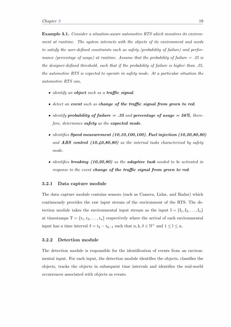
Example 3.1. Consider a situation-aware automotive RTS which monitors its environ-

ment at runtime. The system interacts with the objects of its environment and needs

to satisfy the user-defined constraints such as safety (probability of failure) and perfor-

mance (percentage of usage) at runtime. Assume that the probability of failure = .25 is

the designer-defined threshold, such that if the probability of failure is higher than .25,

the automotive RTS is expected to operate in safety mode. At a particular situation the

automotive RTS can,

• identify an object such as a traffic signal.

• detect an event such as change of the traffic signal from green to red.

• identify probability of failure = .35 and percentage of usage = 56%, there-

fore, determines safety as the expected mode.

• identifies Speed measurement (10,10,100,100), Fuel injection (10,20,80,80)

and ABS control (10,40,80,80) as the internal tasks characterized by safety

mode.

• identifies breaking (10,20,80) as the adaptive task needed to be activated in

response to the event change of the traffic signal from green to red.

3.2.1 Data capture module

The data capture module contains sensors (such as Camera, Lidar, and Radar) which

continuously provides the raw input stream of the environment of the RTS. The de-

tection module takes the environmental input stream as the input I = {I1, I2, . . . , In}

at timestamps T = {t1, t2, . . . , tn} respectively where the arrival of each environmental

input has a time interval δ = tk − tk−1 such that n, k, δ ∈ N+ and 1 ≤ l ≤ n.

3.2.2 Detection module

The detection module is responsible for the identification of events from an environ-

mental input. For each input, the detection module identifies the objects, classifies the

objects, tracks the objects in subsequent time intervals and identifies the real-world

occurrences associated with objects as events.

Chapter 3 20

Object identifier

Object classifier

Object tracker

Event identifier

Data capture

moduleDetection module

Event properties

extractor

Event classifier

Analytics

module

S1 SnS2

…

Characterization of

situations

Environmental

input stream

Figure 3.1: Components of operational environment model of the situation-awarereal-time system.

3.2.2.1 Object identifier

We use the inputs obtained from the sensors (such as Lidar, Radar and Camera) to

detect an object and identify different properties associated with the object from the

RTS environment. We use the Lidar sensor to determine the location of an object and

measure the distance of the object from the RTS. To measure the distance, we illuminate

the object with pulsed laser light and use the Lidar sensor to measure the reflected pulses.

The wavelengths and the laser return time differences are used to identify the type of

the object. Hence, we use Lidar to determine the object type, location, and distance of

the object from the RTS.

We use RADAR to detect objects within a specified range, and identify the location,

object type along with the distance of the object from the RTS. The RTS considered

in this work, also uses a camera to identify objects from its environment. We use

the video data obtained from the camera as an input. To identify an object, we use the

convolutional neural network which consists of two types of layers such as Convolutional,

and Fully-Connected. In this work, for identifying an object, we use nine convolutional

layers followed by two connected layers. Although the detection and classification occur

at runtime, training the neural network is performed offline using the ImageNet dataset.

We identify the object type, location, and the distance of the object from the RTS.

Sensor fusion is the approach for combining the data obtained from different sensors

so that the resulting information is more accurate in comparison to the data which

are individually obtained from the sensors. Each sensor provides three properties of

an object such as object type, location, and the distance of the object from the RTS

Chapter 3 21

which is combined using sensor fusion as presented in Figure 3.1. For each property, we

combine the sensor inputs using the Central Limit Theorem. We apply sensor fusion to

determine all the properties associated with an object and thereby detect an object.

3.2.2.2 Object classifier

For each detected object Ob, the object classifier presented in Figure 3.1 is responsible

predicting the conditional class probability. For each environmental input, we classify

the objects using CNN (which has been train on ImageNet dataset) at runtime. For each

object Ob, we record the information which includes unique identification number of the

object, the recorded time, location, state (like moving or static object in Example 3.1)

and the speed of the object.

The RTS can interact with the objects at runtime and may need to execute additional

operations due to these interactions. The operational environment model also detects

events associated with the objects by tracking the objects as shown in Figure 3.1.

3.2.2.3 Object tracker

The next step of the detection module is to track and match the objects in the current

environmental input with the objects identified in the previous environmental input.

Algorithm 1 presents the steps and methodologies involved in tracking and matching

objects for each newly arrived environmental input. When In+1 becomes the current

environmental input, the object tracker identifies the locations of all the objects. For

each object Ob in In, object tracker defines a variable called FDL (in Line 5 of Algo-

rithm 1) which denotes the maximum possible distance between two objects. The object

tracker compares Ob with all the objects in In+1 (in line 6 of Algorithm 1). Line 7 of

Algorithm 1 defines function called distance(Ob,Ob′) which calculates the distance be-

tween two objects, Ob in In and Ob′ in In+1. The object tracker calculates minimum

distance called LD by comparing Ob in In with all the objects in In+1. If the minimum

distance is less than some pre-defined threshold TH, object tracker considers them as

the same object by matching their id (as presented in line 13 and 14 of Algorithm 1).

On the other hand, for the detected object Ob′ in In+1, if Ob′ .least distance is greater

than threshold TH, the object tracker identifies it as a new object detected in In+1 (as

shown in line 16 of Algorithm 1).

Chapter 3 22

Algorithm 1 Tracking and matching objects

1: procedure Track-And-Match-Objects(In, In+1)2: OIn ← {On

1 , . . . ,Onq}, ∀(1 ≤ i ≤ q) : Ob ∈ In

3: OIn+1 ← {On+11 , . . . ,On+1

r }, ∀(1 ≤ j ≤ r) : Ob′ ∈ In+1

4: for all object Ob ∈ OIn do5: Ob.least distance← FDL6: for each object Ob′ ∈ OIn+1 do7: LD← distance(Ob,Ob′)8: if LD ≤ Ob.least distance then9: Ob.least distance← LD

10: Index← Ob′ .id11: end if12: end for13: if Ob.least distance ≤ TH then14: Ob.id← Index15: else16: OIn+1 ← OIn+1 ∪Ob

17: end if18: end for19: end procedure

Similarly, to determine any changes or modifications of the object behavior in the current

environmental input, for each arriving environmental input, object tracker compares

each object Ob′ in In+1 with its previous condition in In. The object tracker considers

that Ob′ did not undergo any significant modification or change when the difference is

less than a threshold value (predefined) TH. However, if the difference is more than

the predefined threshold, object tracker detects the change for the particular object.

Therefore, object tracker can determine any changes in the behavior of the object. For

example, in the automotive system presented in Example 3.1, changes in the location of

the vehicle or pedestrian can be determined, or any variations in the color of the traffic

light can be identified.

3.2.2.4 Event identifier

The event identifier defines an event Ec as the actions, changes or interactions with one

or more objects. One of the essential tasks in the characterization of an environmental

situation is the detection of events. In this thesis, the detection of events involves using

Algorithm 1 to track various objects and identification of changes in their properties.

With the arrival of new environmental input, any changes associated with an object is

identified as an event.

Chapter 3 23

Events that are associated with objects can be detected by the operational environment

model from the environmental input stream through tracking. The event identifier uses

a temporal data called ED and stores the information of the events related to the objects

which can be defined as,

ED = (x1, x2, . . . , xu) (3.1)

Where u is a natural number such that u ∈ N+. For each event Ec, in this thesis,

the event identifier stores properties which include location, state, and speed in ED at

different timestamp. Therefore, ED contains information regarding the events associated

with each object and keeps track of the changes in its position and state recorded at

different times.

3.2.3 Analytics module

An RTS can experience failure if the timing constraints are not adequately met. There-

fore, exact calculations of timing constraints associated with the events are essential.

It is also necessary to detect real-time and non real-time properties associated with an

event. The analytics module is responsible for performing different steps which are the

extraction of the properties of an event, classification of events based on their real-time

properties and characterization of the environmental situations in terms of events as

illustrated in Figure 3.1.

3.2.3.1 Event properties extractor

The analytics module extracts both real-time and non real-time properties associated

with an event from the environmental input stream. For each event, the analytics module

identifies its properties which include location, state, and speed using ED in different

timestamps. The analytics module also uses ED to calculate the duration of each event

which is the difference between the start time of an event with its completion time (or

the time when it has moved out of the environmental input stream). For each event Ec,

we identify the start time of an event and its duration using ED defined in Equation 3.1.

Duration Ec.duration for any event Ec can be represented as:

Ec.duration = Ec.endtime− Ec.starttime (3.2)

Chapter 4 24

Where, Ec.starttime and Ec.endtime are respectively the timestamp of start and end

time of Ec. We use ED for identifying the periodicity of the events. We analyze ED

at runtime and keep track of appearance of the events in different timestamps. For a

particular event Ec, PE is the period of the event if,

Ec.timestamp = Ec.(timestamp + PE) (3.3)

3.2.3.2 Event classifier

The analytics module also uses ED to determine the occurrence patterns of the events.

The analytics module continuously analyzes the events, uses ED to determine its previ-

ous occurrences and detects whether an event is periodic or not. The module classifies

each event into two categories: (1) periodic and (2) aperiodic. If the event takes place

without maintaining any consistency, it can be categorized as an aperiodic event. When

an event takes place after a fixed interval, we define the event as periodic. For a periodic

event, the analytics module also determines its periodicity.

3.2.3.3 Characterization of situations

For each event, we store its state, location, speed, duration, and periodicity (for the

aperiodic event, the periodicity value is zero). At a particular timestamp tk, we char-

acterize the environmental situation as the collection of events detected at that time as

presented in Figure 3.1. In timestamp tk, situation Sk can be represented as,

Sk =

Situation︷ ︸︸ ︷tk,E1,E2, . . . ,Ed (3.4)

Where d is the number of detected events in situation Sk, tk is the timestamp when the

situation was captured and {E1,E2, . . . ,Ed} are the detected events at tk.

Chapter 4

Mapping situations to tasks in the

situation-aware real-time system

4.1 Introduction

A situation-aware RTS needs to have sufficient knowledge of its situations and its sub-

sequent changes, which can be obtained from the environmental input stream [45]. It

is necessary for the system to have a prior knowledge of its interactions with various

objects of the environment involving different timing constraints to ensure safe and

correct operations. It is also essential for the system to extract timing properties by

mining environmental input data, and understand the flow of execution by creating a

knowledge-base. Therefore, one of the aims of the situation-aware RTS is to create a

knowledge-base from the monitored environmental input stream that will consume sig-

nificantly less memory, allow faster information processing, and help to identify, analyze

and validate safety, performance as well as adaptive aspects.

4.2 Workflow of the situation-aware real-time system

The complexity of existing RTS and available adaptive behaviors have led the RTS re-

search community to investigate innovative ways of designing and developing a situation-

aware RTS which can assure functional as well as timing guarantees at runtime. The

RTS can undergo a number of interactions with various objects of the environment which

create challenges for predicting and assuring the runtime behavior. Failures of such sys-

tem at runtime can result in death, potential harm to property, or the environment [46].

25

Chapter 4 26

For the RTS, situation-awareness is emerging as a necessary underlying ability which

creates the necessity for designing innovative ways to ensure its smooth operation at

runtime.

4.2.1 Monitoring the environment of the real-time system

Monitoring the environmental situations of the RTS [47] is useful for validating the func-

tional and timing requirements of RTS. Interestingly, monitoring can gather information

about the environment which is essential to investigate uncertainties [48] towards build-

ing an intelligent RTS that has sufficient knowledge of all the possible interactions. The

RTS can use the environmental input stream gathered from the monitored environment

to identify data patterns [48] which can help in characterizing the situations including

the uncertainties of the system environment.

4.2.2 Characterizing environmental situation

One of the objectives of the proposed situation-aware RTS is to characterize the en-

vironmental situation which includes identification of real-world occurrences as events

from mining the monitored environmental input stream and analyzing their properties.

The properties of the events also allow us to create a knowledge-base which presents in-

formation about historical as well as current environmental situations in terms of events

(along with their properties and relationships involved among them). It also facilitates

faster information retrieval and processing, allowing the RTS to compute a significant

amount of environmental information with limited overload.

4.2.2.1 Identifying objects and events

The initial steps for characterizing environmental situation involve the identification and

classification of objects from the environmental input stream obtained from different

sensors. We perform sensor fusion to combine and identify the objects present in the

RTS environment. An identified object Ob, in our work, can be defined as follows:

Chapter 4 27

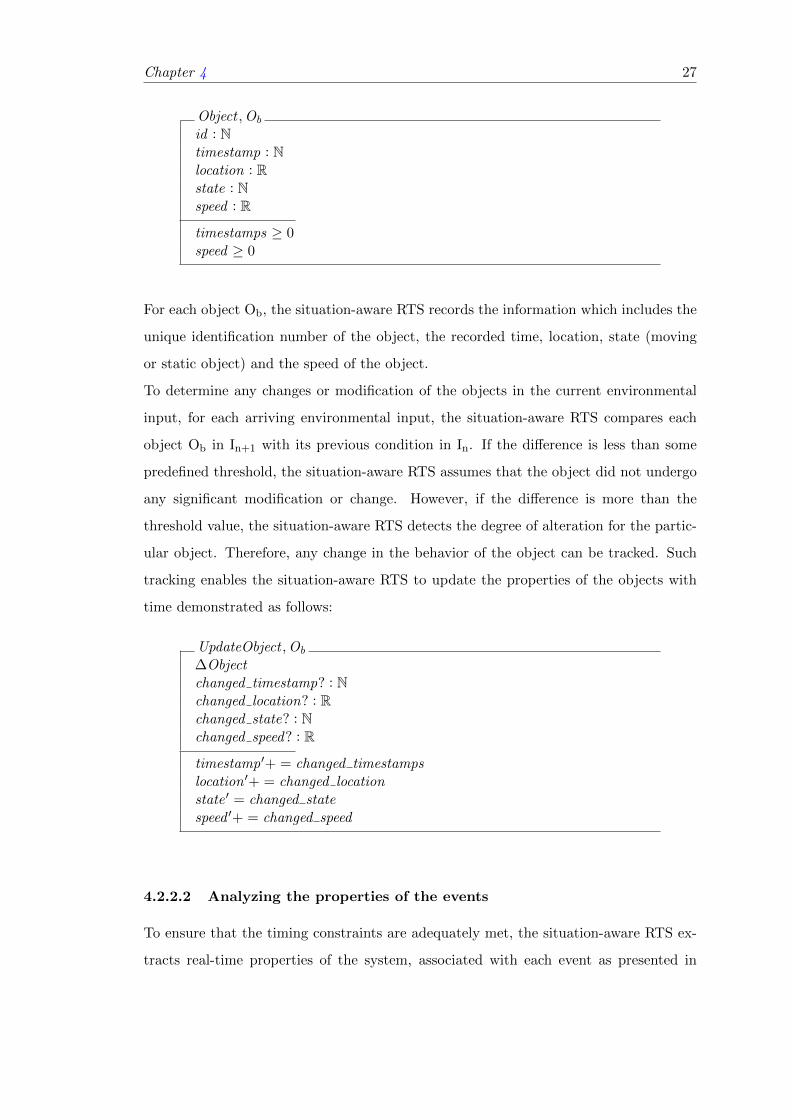
Object ,Ob

id : Ntimestamp : Nlocation : Rstate : Nspeed : R

timestamps ≥ 0speed ≥ 0

For each object Ob, the situation-aware RTS records the information which includes the

unique identification number of the object, the recorded time, location, state (moving

or static object) and the speed of the object.

To determine any changes or modification of the objects in the current environmental

input, for each arriving environmental input, the situation-aware RTS compares each

object Ob in In+1 with its previous condition in In. If the difference is less than some

predefined threshold, the situation-aware RTS assumes that the object did not undergo

any significant modification or change. However, if the difference is more than the

threshold value, the situation-aware RTS detects the degree of alteration for the partic-

ular object. Therefore, any change in the behavior of the object can be tracked. Such

tracking enables the situation-aware RTS to update the properties of the objects with

time demonstrated as follows:

UpdateObject ,Ob

∆Objectchanged timestamp? : Nchanged location? : Rchanged state? : Nchanged speed? : R

timestamp′+ = changed timestampslocation ′+ = changed locationstate ′ = changed statespeed ′+ = changed speed

4.2.2.2 Analyzing the properties of the events

To ensure that the timing constraints are adequately met, the situation-aware RTS ex-

tracts real-time properties of the system, associated with each event as presented in

Chapter 4 28

Discovery of relationship

among events

Analysis of the events

Real-time system

video dataIdentification of derived

events

Extraction of properties

Classification of events

Knowledge-base

Figure 4.1: Identification and analysis of the properties of events

Figure 4.1. We define a temporal dataset called ED, which uses the updated informa-

tion associated with an object Ob and stores its states and properties for each Ik ∈ I.

Therefore, ED keeps track of various activities associated with each object, which serves

as the basis of event detection. The situation-aware RTS uses ED to identify an event

Ec associated with an object Ob. For each event Ec, the situation-aware RTS identifies

the start time of the event and determines its duration using ED. The situation-aware

RTS also perform continuous analysis of the detected events on ED and capture the

appearances of events in different timestamps.

Event ,Ec

id : NinteractingObject : PObjectstartTime : NendTime : Nduration : Nlocation : Rspeed : Rtype : P periodic, aperiodic

duration = endTime − startTime;

Event Ec contains information regarding the events associated with each object. The

situation-aware RTS uses Ec to keep track of the changes of the event in terms of position

and state with respect to time.

Chapter 4 29

4.2.2.3 Identifying the relationships involved among events

Apart from the detection of the events associated with different objects, the situation-

aware RTS also identifies those events that are the results of interactions between two

or more events as shown in Figure 4.1. The situation-aware RTS classifies the events

as basic set of events called Ebasic and derived set of events called Ederived. Derived

events occur because of the interactions among the basic events. The situation-aware

RTS contains a dataset called AR which contains the association relationships among

the Ebasic and Ederived. Each row ARi ∈ AR contains a set of events E (that are in

association with each other) and a rule, which has the following form,

Ebasic ⇒ Ederived, Where Ebasic,Ederived ⊆ E

Each row ARi ∈ AR represents a rule in terms of events. However, from all rules in

AR, the situation-aware RTS identifies the rules which are valid and selects them while

determining the derived events. Hence, for each set of event Ebasic, the situation-aware

RTS identifies its frequency in AR using the function fr(Ebasic) which can be represented

as,

fr(Ebasic) =

∣∣{ARi ∈ AR; Ebasic ⊆ ARi}∣∣

|AR|(4.1)

For each rule, the situation-aware RTS uses AR to identify how often the rule was

evaluated as true using the confidence value. The situation-aware RTS calculates the

confidence value conf(Ebasic ⇒ Ederived) as the ratio of the transactions which contain

Ebasic with the transactions containing Ederived.

conf(Ebasic ⇒ Ederived) =fr(Ebasic ∪ Ederived)

fr(Ebasic)(4.2)

For each rule, the situation-aware RTS also identifies a conviction value. The conviction

value conv(Ebasic ⇒ Ederived) can be defined as the ratio of the frequency where Ebasic

takes place without Ederived (i.e., the possibility of making an incorrect prediction).

conv(Ebasic ⇒ Ederived) =1− fr(Ederived)

1− conf(Ebasic ⇒ Ederived)(4.3)

From all possible rules, the situation-aware RTS considers only those rules that satisfy

a minimum confidence value and maximum conviction value. The rules which satisfy

the thresholds is considered as the set of final rules and stored in AR to determine the

Chapter 4 30

derived events at runtime. An event must take place if every other event it is associated

with takes place.

Example 4.1. Derived event: Assume a row of AR contains events E1, E2, E3 and E4

associated with each other. The situation-aware RTS concludes that event E4 (although

it may be undetected) must take place if we detect E1, E2 and E3. In this case E1, E2

and E3 can be termed as basic events and E4 can be identified as derived events.

UpdateEvent ,Ei

∆Eventchanged timestamps? : Nchanged location? : R

timestamps ′+ = changed timestampslocation ′+ = changed location

4.2.3 Creating the knowledge-base

Data helps us in understanding the patterns and relationships involved among the de-

tected events from the environment of an RTS. The RTS can identify the safety and

performance constraints as well as analyze the historical and current information to

make a deterministic prediction of its future conditions. Therefore, it is necessary to

generate a knowledge-base which describes the environment of the RTS in terms of

events. It is also required to ensure that the generated knowledge-base consumes signif-

icantly reduced memory and allows faster computation such that it is suitable for the

RTS. Our proposed formation of a knowledge-base scheme is presented as follows:

• For each input Ik, the situation-aware RTS identifies all the events using temporary

data called ED defined in Equation 3.1.

• For each event Ec, the situation-aware RTS uses the operational environment

model to extract its properties and determines whether it is a newly arrived event

or an existing event.

• For each existing event, the situation-aware RTS determines its type (periodic or

aperiodic). In case of periodic events, the module determines its periodicity.

• The situation-aware RTS uses AR to detect derived events from basic events.

• The situation-aware RTS presents a knowledge-base which is called KB as shown

in Figure 4.1.

Chapter 4 31

• If the detected event is newly arrived or aperiodic, the situation-aware RTS stores

its information (along with its properties) in KB.

• If the event is periodic, the situation-aware RTS avoids storing the event (as its

first occurrence is already stored).

• If the event is a derived event, consisting of a combination of basic events, the

situation-aware RTS avoids storing the basic events which are already stored.

The situation-aware RTS identifies the current location of the events, and by comparing

with the past event information, determines their speed and next predicted position.

Apart from the detected event, the situation-aware RTS uses ED and AR formed to

identify the derived events that are the result of existing events. The situation-aware

RTS forms a knowledge-base called KB where it stores all the events detected in each

timestamp of environmental input arrival. In the generated knowledge-base KB, kth

row, KBk can be given as,

KBk = [tk,E1,E2, . . . ,Ed] (4.4)

Where, d is a positive natural number denoting the number of events detected in tk.

Here tk is the timestamp of environmental input arrival and {E1,E2, . . . ,Ed} is the set of

detected events at that timestamp. Since the RTS considered in this work is embedded

in nature, we put a limit on the number of timestamps can be stored in KB. Therefore,

the KB contains a user-defined number of most recent timestamps. In other words, KB

can be considered as a queue of situations where the situations are stored in KB using

the First-In-First-Out replacement policy. In this work, the maximum size of KB is

30,000.

4.2.4 Satisfying the user-defined constraints

The behavior of an RTS can be modeled by a discrete-time finite automaton (5) tuple,

(µ,Σ, ω, µ1,F′), consisting of,

• A finite set of states or modes µ,

• A finite set of events called the alphabet (Σ),

• A transition function based on events (ω : µ×Σ→ µ),

• An initial state or mode (µ1 ∈ µ), and

Chapter 4 32

• A final state (F′ ∈ µ).

The validation framework of the situation-aware RTS determines the expected system

mode µexpected ∈ µ, checks whether the system is operating in the desired mode or not

and triggers a verification action ω (if necessary). The RTS uses ω for switching the

operating mode to µexpected at runtime. To model the mode changes of the RTS, we

define an event variable containing two event values, Σ = {up, down}. The transition

functions are defined by,

1. safety = ω(performance, up)

2. performance = ω(safety,down)

4.2.5 Identifying adaptive tasks in a particular situation

In this thesis, we identify additional adaptive tasks obtained from the environmental

situations at runtime. For each situation, the RTS identifies the environmental events

and determines their properties (such as duration, location, speed, and periodicity).

Therefore, the RTS can collect information on the system behavior at runtime through

monitoring and allows characterization of behavior regarding each experienced situation.

For each situaion Sk, Algorithm 2 uses the procedure IdentifyAdaptiveTasks(Sk) to iden-

tify a set of d events associated with different objects Sk = {E1,E2, . . . ,Ed}. Each event,

in our work, can be categorized into one of discrete categories γ = {γ1, γ2, . . . , γg}. The

procedure IdentifyAdaptiveTasks(Sk) identifies the unique visited catogories assiocited

with the events detected in Sk.

Each event category γi corresponds to a particular adaptive task τi. The procdure

FindAdaptiveTasks(γi) in Algorithm 2 performs decision rule learning (from line 16 to

21) and identifies the adaptive taskset associated with the events and uses procedure

FindDepandantTasks(τi) to identify the dependant tasks.

We define a dataset called PR which contains precedence relationship τi ⇒ τj (denotes

every occurrence of τj must be preceded by τi) among the adaptive tasks. For each

identified tasks τouti , we also use PR to identify addition adaptive tasks which precede

τoutk . Therefore, for a particular situation Sk, Algorithm 2 identifies the adaptive tasks

τSkout which are needed to be executed.

Chapter 4 33

Algorithm 2 Identify adaptive tasks from a situation.

1: procedure IdentifyAdaptiveTasks(Sk)2: τSkout ← ∅3: VisitedEventCategory← ∅4: for each Event Ej ∈ Sk do5: γj ← Occurrencecategory(Ej)6: γj.visited← Find(VisitedEventCategory, γj)7: if γj.visited = false then8: FindAdaptivetasks(V, vj)9: VisitedEventCategory.add(γj)

10: end if11: end for12: end procedure13: procedure FindAdaptiveTasks(γi)14: τadaptive ← ∅15: f(γi) =

∣∣{TDi ∈ TD; γi ⊆ TDi}∣∣ /|TD|

16: for each task τi ∈ τout do17: cf(γi ⇒ τi) = f(γi ∪ τi)/f(γi)18: cv(γi ⇒ τi) = (1− fr(τi))/(1− cf(γi ⇒ τi))19: if cf ≤ FH ∧ cv ≤ VH then20: τadaptive ← τadaptive ∪ FindDepandantTasks(τi)21: end if22: end for23: return τadaptive24: end procedure25: procedure FindDepandantTasks(τi)26: τi.visited← true27: for each Vertex τj ∈ PR[τi.Parent] do28: if τj.visited = false then29: FindDepandantTasks(τj)30: end if31: end for32: return τdependant ∪ τj33: end procedure

4.2.6 Execution model of the proposed situation-aware real-time sys-

tem

The proposed situation-aware RTS contains two types of execution model which are

non-adaptive and adaptive execution models as presented in Figure 4.2.

1. Non-adaptive execution model: In non-adaptive execution model, the RTS executes

only tasks from internal task set characterized by current mode. The RTS can use a

scheduler characterized by a scheduling algorithm called SA1 such that SA1 : τµcurrentin → Pr

(assigns and executes each task τi ∈ τµcurrentin using a processor Pr) as illustrated by Fig-

ure 4.2. In this work, we consider SA1 = EDF, ( i.e. the non-adaptive execution model

Chapter 4 34

uses the EDF scheduling algorithm) for scheduling the internal tasks.

Adap

tive

exec

uti

on m

odel

No adaptation

Evaluation of

the tasks

Yes

No

Har

dw

are

Processor

Scheduler

Internal task set

τs1 τs2 τsq

….Appli

cati

on

Adaptive task set

τ1 τ2 τr

….

Non

-adap

tive

exec

uti

on m

odel

….

Identification of

the execution order

GM

FN

C-G

MFD

esig

ner

input

RB

RR

TN

C-R

RT

SA

TM

τ1

τ2

τo

Saf

ety

mode

τp1 τp2 τpm

….

Per

form

ance

mode

Figure 4.2: Execution model of the situation-aware RTS

2. Adaptive excution model: In adaptive execution model, we identify events in differ-

ent situations and execute adaptive tasks in response to the events that take place in

the RTS environment. The adaptive execution model is characterized by a scheduling

algorithm SA2 : {τµcurrentin ∪ (τout ⊆ G)} → Pr such that it assigns the both the inter-

nal and the adaptive task τi ∈ {τµcurrentin ∪ τout} in processor Pr in order to execute all

the tasks. Figure 4.2 shows that the RTS designer can select any task model from

{GMF,NC−GMF,RB,RRT,NC− RRT, SATM} for the execution of adaptive tasks.

4.2.7 Using existing task models to execute adaptive tasks

Our execution model allows the tasks to be included in the existing task model if the

schedulability analysis associated with the task model are met.

One of the primary challenges in developing these models is their analytical complexity.

More specifically the graph-based models are difficult to analyze. For a set of adaptive

tasks τout, the adaptive execution model presented in Figure 4.2 calculates the accu-

mulated worst-case execution demand rfτout(δ) of τout that can be released in δ due to

the events detected in Sk. The adaptive execution model allows the designer to select

any one task model from {GMF,NC−GMF,RB,RRT,NC− RRT,SATM}. For each

selected task model, we perform a schedulability test using their respective feasibility

analysis procedure defined in [49]. The adaptive execution model allows the selected task

model to execute the adaptive task τout identified in Sk, if τout pass the schedulability

test.

Chapter 4 35

4.3 Proposed situation-aware graph-based task model

We present SATM, which allows the execution of adaptive tasks in different environ-

mental situations. Each task can be added to the proposed SATM dynamically as a

vertex and the execution order between a pair of tasks as an edge. While including the

adaptive tasks in SATM, we ensure timing requirements by defining a number of timing

and graph-based constraints and include the vertices in the SATM, if the constraints are

met. In a particular situation Sk, the adaptive tasks in SATM can be characterized by

a directed acyclic graph G(Sk) which can be defined as:

G(Sk) = (V,H) where,

1. V is the set of vertices. For each Sk, the RTS needs to execute a set of adaptive

tasks τSkout ∈ τout. Each task τouti ∈ τSkout is represented using a vertex vi ∈ V.

2. Each vertex vi ∈ V can be defined as, vi = (αi,Ci,Di).

3. H is the set of directed edges. Each edge (vi, vi+1) represents the order of execution

of two tasks (τouti , τouti+1).

4.3.1 Characterizing adaptive tasks using SATM

For each situation Sk, we identify the set of vertices V = {v1, v2, . . . , vr} needed to be

executed in response to events detected in Sk by performing decision rule learning. For

each event Ej in Sk, we identify the vertex vi ∈ V needed to be executed. We identify

whether vi is already included in the SATM. We define a set called CV which stores

the vertices that can potentially be added to the SATM in the current situation. If vi

is absent in the SATM and CV, we add it to CV. We use PR to identify the vertices

which precede vi and also add them to CV. Other events which have the same occurrence

pattern can also be translated to the same adaptive task. Hence for a particular situation

Sk, we identify the set of tasks τSkout which are needed to be executed.

4.3.2 Evaluating timing constraints

A task must complete its execution within a specific time bound. Hence, it is essential

for the RTS to define and evaluate various timing constraints associated with each vertex

before including it in the SATM. The constraints are described as follows:

Chapter 4 36

1. Deadline constraint, TC1(vi): Each vertex vi must finish its execution before

the deadline Di.

Ci ≤ Di (4.5)

2. Real-time task order, TC2(vi, vi+1): A vertex vi can precede (execute before

another) another vertex vi+1 iff, the relative deadline of vi is less than or equals

to the the relative deadline of vi+1.

Di ≤ Di+1 (4.6)

3. Range, TC3(vi): The worst-case execution time demand of vertex vi must satisfy

range Tavailable defined in Equation 4.

θ(τin) =∑i∈q

Ci (4.7)

Tavailable = δ − θ(τin) (4.8)

4. Estimated duration, TC4(vi): The estimated duration ∆(vi) for each vertex

vi ∈ V must be less than Tavailable.

∆(vi) ≤ Tavailable (4.9)

For a set of tasks to be evaluated as correct, no timing constraints can be violated which

we define as TC. Therefore, for each situation Sk, evaluation of the timing constraints

associated with each vertex vi ∈ V can be represented as,

TC1(vi) ∧ TC2(vi, vi+1) ∧ TC3(vi) ∧ TC4(vi) � TC (4.10)

4.3.3 Evaluating graph-based properties

Graph-based properties, GC: During the formation of the SATM, the mapped ver-

tices must follow some graph-based properties which are described below:

GC1: A pair of vertices (vi, vi+1) can form an edge if they satisfy Equation 4.11.

Di+1 − Ci+1 − αi+1 ≥ Di − Ci − αi (4.11)

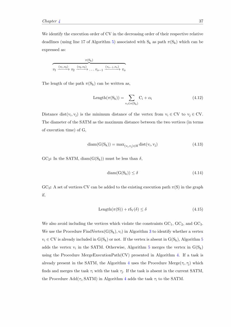
Chapter 4 37

We identify the execution order of CV in the decreasing order of their respective relative

deadlines (using line 17 of Algorithm 5) associated with Sk as path π(Sk) which can be

expressed as:

π(Sk)︷ ︸︸ ︷v1

(v1,v2)−−−−→ v2(v2,v3)−−−−→ . . . vo−1

(vo−1,vo)−−−−−−→ vo

The length of the path π(Sk) can be written as,

Length(π(Sk)) =∑

vi∈π(Sk)

Ci + αi (4.12)

Distance dist(vi, vj) is the minimum distance of the vertex from vi ∈ CV to vj ∈ CV.

The diameter of the SATM as the maximum distance between the two vertices (in terms

of execution time) of G,

diam(G(Sk)) = max(vi,vj)∈H dist(vi, vj) (4.13)

GC2: In the SATM, diam(G(Sk)) must be less than δ,

diam(G(Sk)) ≤ δ (4.14)

GC3: A set of vertices CV can be added to the existing execution path π(S) in the graph

if,

Length(π(S)) + rfV(δ) ≤ δ (4.15)

We also avoid including the vertices which violate the constraints GC1, GC2, and GC3.

We use the Procedure FindVertex(G(Sk), vi) in Algorithm 3 to identify whether a vertex

vi ∈ CV is already included in G(Sk) or not. If the vertex is absent in G(Sk), Algorithm 5

adds the vertex vi in the SATM. Otherwise, Algorithm 5 merges the vertex in G(Sk)

using the Procedure MergeExecutionPath(CV) presented in Algorithm 4. If a task is

already present in the SATM, the Algorithm 4 uses the Procedure Merge(τi, τj) which

finds and merges the task τi with the task τj. If the task is absent in the current SATM,

the Procedure Add(τi,SATM) in Algorithm 4 adds the task τi to the SATM.

Chapter 4 38

Algorithm 3 Find Vertex in SATM.

1: procedure FindVertex(G(Sk), vi)2: vi.visited← true3: for each Vertex vj ∈ G(Sk).Adj[vi] do4: if vj.visited = false then5: FindVertex(G(Sk), vj)6: end if7: end for8: return vj

9: end procedure

4.3.4 Identifying the execution order of adaptive tasks

For each new event, if the mapped vertex is already included in CV, we avoid including

the vertex in CV. In other words, events considered in this work can be categorized

into one of the discrete categories γ. Each event category γk ∈ γ corresponds to a

particular occurrence pattern which can be mapped to one particular adaptive task.

Hence, multiple events in Sk can be mapped to one particular task.

Algorithm 4 Merge adaptive tasks in Existing task model.

1: procedure MergeAdaptiveTasks(τSkout)2: for each task τi ∈ τSkout do3: τi.visited← false4: end for5: for each task τi ∈ τSkout do6: if (τj ← FindVertex(τSkout, τi)) then7: Merge(τi, τj)8: else9: Add(τi,TaskModel)

10: end if11: end for12: end procedure

For example, consider that the automotive system specified in Example 3.1 identifies

two events in a particular situation such as 1) movement of a pedestrian from one side

of the road to another, and 2) the change of a traffic signal from yellow to red. These

two events can be translated to one adaptive task in the automotive system which is

”Braking.” Therefore, CV contains the vertices which are needed to be executed in Sk.

Since multiple events can be mapped to one particular task, the number of vertices in

CV is less than or equal to the number of tasks in τSkout.

Algorithm 5 illustrates the step by step procedure of identifying the execution order of

CV. We use the respective relative deadlines of all the vertices to assign priorities (in

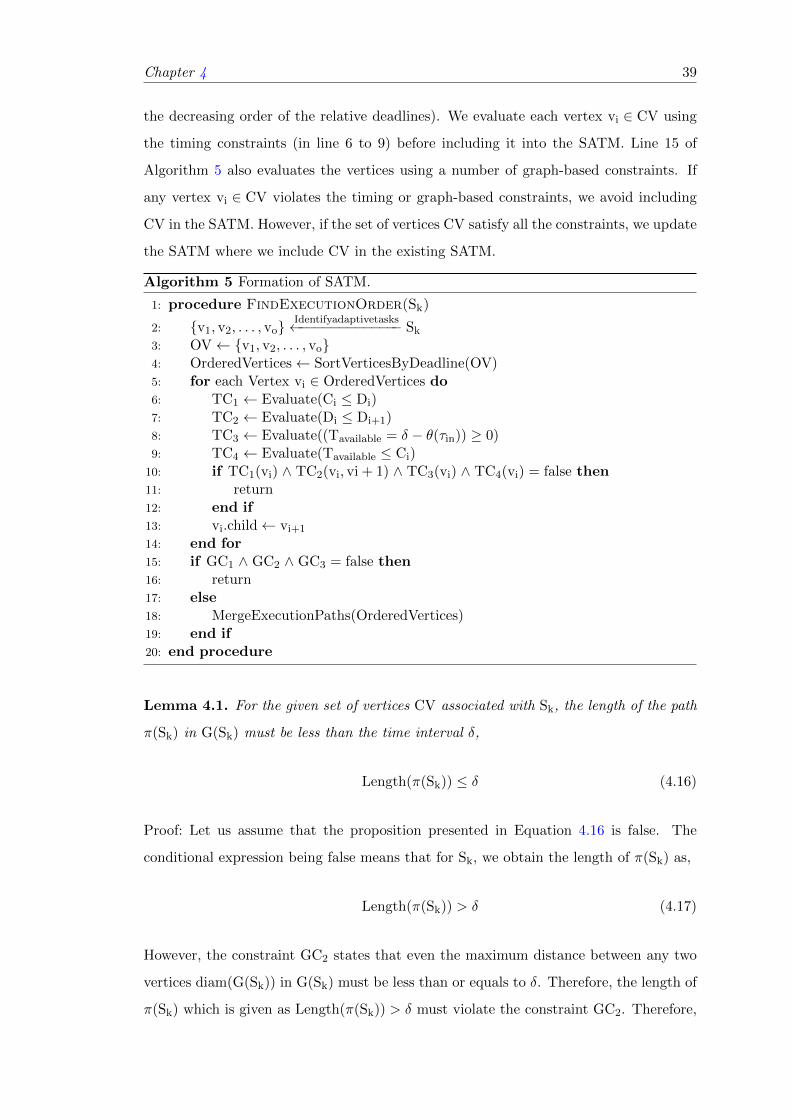
Chapter 4 39

the decreasing order of the relative deadlines). We evaluate each vertex vi ∈ CV using

the timing constraints (in line 6 to 9) before including it into the SATM. Line 15 of

Algorithm 5 also evaluates the vertices using a number of graph-based constraints. If

any vertex vi ∈ CV violates the timing or graph-based constraints, we avoid including

CV in the SATM. However, if the set of vertices CV satisfy all the constraints, we update

the SATM where we include CV in the existing SATM.

Algorithm 5 Formation of SATM.

1: procedure FindExecutionOrder(Sk)

2: {v1, v2, . . . , vo}Identifyadaptivetasks←−−−−−−−−−−−−− Sk

3: OV← {v1, v2, . . . , vo}4: OrderedVertices← SortVerticesByDeadline(OV)5: for each Vertex vi ∈ OrderedVertices do6: TC1 ← Evaluate(Ci ≤ Di)7: TC2 ← Evaluate(Di ≤ Di+1)8: TC3 ← Evaluate((Tavailable = δ − θ(τin)) ≥ 0)9: TC4 ← Evaluate(Tavailable ≤ Ci)

10: if TC1(vi) ∧ TC2(vi, vi + 1) ∧ TC3(vi) ∧ TC4(vi) = false then11: return12: end if13: vi.child← vi+1

14: end for15: if GC1 ∧ GC2 ∧ GC3 = false then16: return17: else18: MergeExecutionPaths(OrderedVertices)19: end if20: end procedure

Lemma 4.1. For the given set of vertices CV associated with Sk, the length of the path

π(Sk) in G(Sk) must be less than the time interval δ,

Length(π(Sk)) ≤ δ (4.16)

Proof: Let us assume that the proposition presented in Equation 4.16 is false. The

conditional expression being false means that for Sk, we obtain the length of π(Sk) as,

Length(π(Sk)) > δ (4.17)

However, the constraint GC2 states that even the maximum distance between any two

vertices diam(G(Sk)) in G(Sk) must be less than or equals to δ. Therefore, the length of

π(Sk) which is given as Length(π(Sk)) > δ must violate the constraint GC2. Therefore,

Chapter 4 40

path π(Sk) for which conditional expression 4.17 is true cannot exist in the SATM. Thus

the proposition presented in Equation 4.16 must be true.

Lemma 4.2. A new path π(Sk) can be merged to an existing execution path π(S) in the

graph if,

Length(π(S)) + Length(π(Sk)) ≤ δ (4.18)

Proof: Merging the execution paths in Algorithm 5 consist of two cases. Case one

involves finding and matching the vertices which are present in both π(Sk) and π(S). In

this case, since no new vertices are added in path π(S) we have,

Length(π(S)) + Length(π(Sk)) = Length(π(S)). Hence, using Lemma 1, we can state

that the overall length of the execution path Length(π(S)) is less that δ.

Case two includes those vertices which are present in π(Sk), but absent in π(S) and

thereby requires the addition of new vertices. From GC3, we see that adding new

vertices in the existing path π(S) also keeps the overall length less than δ.

Example 4.2. Formation of SATM: Assume that, we capture a situation S1 at

runtime. Also, consider that the system needs to execute adaptive tasks (τ1, τ2, τ3, τ4)

in response to S1 with relative deadlines (2, 9, 37, 18) respectively. Our system con-

structs a SATM which contains each task as vertex and flow (order) of execution be-

tween them as edges. Therefore, it constructs the graph model which executes the tasks

in (τ1 → τ2 → τ4 → τ3) order.

τ1 τ2 τ4 τ3S1 S1 S1

Additionally, consider that we obtain new situations at runtime which are associated

with following adaptive tasks,

• S2 = (τ1, τ6, τ4, τ3)

• S3 = (τ2, τ1, τ3, τ5)

• S4 = (τ2, τ1, τ4, τ5, τ3)

If the tasks τ5, and τ6 have relative deadlines 32, and 5 respectively, then the final SATM

in after receiving S4, in this example can be visualized as,

Chapter 4 41

τ1 τ2

τ6 τ4

τ5

τ3

S1, S3, S4

S2

S3, S4

S1

S2 S1, S2, S4

S4

S3

In the SATM, for each situation in which the adaptive tasks have satisfied the constraint,

we update the SATM by including the vertices associated with the situation as the new

vertices as presented in Algorithm 5. With the arrival of a new situation Sk at time

tk ∈ T, we determine the overload of the internal tasks τin at first and calculates the

worst-case estimated duration for the internal tasks as, θ(τin). In this work, we consider

the frame arrival time tk as the scheduling point and schedule the ready tasks in time

interval δ (supply).

4.3.5 Schedulibility analysis of adaptive tasks for each situation

Theorem 4.3. If the initial input to Algorithm 5 is G(Sk) and the finally constructed

SATM is G(S′k) then,

Length(π(Sk)) ≥ Length(π(S′k))

Proof: Consider that CV is the set of vertices obtained at runtime and CV′ is the

set of vertices which satisfies the constraints. Assume that, the RTS avoids execution

of r number of adaptive tasks from the given situation where (r ≥ 0) which can be

represented using adaptive task set, vr = vi : (0 ≤ r ≤ card(CV′)). Therefore, we have,

CV = CV′ ∪ vr (4.19)

The cardinality of these task sets can be viewed as:

card(CV) = card(CV′) + card(vr)

⇒ card(CV) ≥ card(CV′)

Chapter 4 42

From the above expression, we view that system avoids execution of vr form a set of

G(Sk) vertices and executes G(S′k) tasks.

∆(CV) =∑

vi∈CV

Ci, ∆(CV′) =∑

vj∈CV′

Cj, ∆(vr) =∑vk∈vr

Ck

Hence, Equation 4.19 can be written as,

∆(CV) = ∆(CV′) + ∆(vr)∑vi∈CV

Ci =∑

vj∈CV′

Cj +∑vk∈vr

Ck

Since all the vertices are associated with the events captured from the same situation,

they have the same arrival time. So the above expression can be rewritten as,

∑vi∈CV

Ci + αi =∑

vj∈CV′

Cj + αj +∑vk∈vr

Ck + αk

Length(π(Sk)) = Length(π(S′k)) + Length(π(vr))

The vertex set vr has positive or zero number of vertices. Therefore, each vertex vi ∈ vr

has a computation time Ci which is greater than zero. The respective execution paths

associated with the vertices can be represented as,

Length(π(Sk)) ≥ Length(π(S′k))

Theorem 4.4. At a particular situation Sk, with time interval δ, a set of tasks τ = τin ∪G(Sk)

which are being executed using SATM, are uniprocessor feasible.

Proof: From [14] we know that, a set of tasks τin is uniprocessor feasible in a time

interval δ, if dbfτin(δ) < δ. For each δ, a given set of vertices CV can be scheduled after

scheduling all the internal tasks in the Tavailable time slots. Similarly, we know that a

set of vertices G(Sk) is uniprocessor feasible in time interval Tavailable if,

rfG(Sk)(δ) ≤ Tavailable (4.20)

To be considered for execution using SATM, in our work, both internal and adaptive

tasks, for a given situation Sk must satisfy, Tavailable + θ(τin) ≤ δ to be scheduled in a

Chapter 5 43

processor. Hence, the set of tasks τ = τin ∪G(Sk) we have,

dbfτin(δ) + rfG(Sk)(δ) ≤ δ (4.21)

Hence, the combined execution demand associated with the internal and adaptive tasks

never exceeds the supply. Therefore, set of tasks τ = τin ∪G(Sk) are uniprocessor feasi-

ble.

4.4 Discussion

For each situation Sk, the SATM schedules the internal tasks τin at first. Additionally,

the RTS uses the SATM to identify and execute the adaptive tasks τout to the available

slots Tavailable. Therefore, the overall demand (for both internal and adaptive tasks) is

always less than or equals δ (maximum supply). If the tasks associated with the events

satisfies the timing constraints and are already included in the SATM, then the execution

model uses the SATM to execute the tasks at runtime. If the tasks are absent in the

SATM, it avoids executing them at that time, stores their information and performs an

update on the SATM. The formation and update of SATM, in this thesis, are performed

offline because we consider handling the learned situation after tasks associated with the

situation are added to the task model.

Chapter 5

Analyzing user-defined

constraints for the

situation-aware real-time system

5.1 Introduction

In this Chapter, we present a validation framework that identifies the expected mode at

runtime and checks whether the situation-aware RTS is operating in the correct mode

or not. To determine the expected mode, the validation framework identifies the safety

constraint by determining the probability of failure in each environmental situations and

uses the probability of failure of the system to determine the expected mode in different

environmental situations.

The user-defined constraints of a situation-aware RTS must be guaranteed at runtime.

Therefore, it is necessary for the RTS to form a knowledge-base which consumes a

reduced memory and provides an improved decision-making ability (in comparison to

raw environmental input stream). The knowledge-base can be used to identify the

safety and performance of the system in different environmental situations. The goal of

this chapter is to present a validation framework which identifies the expected operating

mode, checks whether the system is operating in the expected mode or not, and triggers a

verification action such that the RTS can satisfy the user-defined safety and performance

constraints by switching its operating mode (if necessary) at runtime.

44

Chapter 5 45

5.2 Identifying the safety constraint

In this thesis, we use KB to perform an analysis of the system from safety perspectives.

To ensure that system states are safe, we perform a deductive failure analysis using fault

tree. Fault tree of the automotive system mentioned in Example 3.1 is illustrated using

Figure 5.1.

Vehicle failure

Accident

Component failureCollision between

moving objects

Traffic signal failure

Event i Event j

Failure of unknown events

Figure 5.1: Our approach for RTS failure analysis using fault tree

A fault tree can be used to analyze one undesirable top event. For an automotive RTS,

in Example 3.1, the top event can be defined as the occurrence of accidents. Once

the top event is identified, now we need to determine the causes along with associated

probabilities for the events. Those can be defined as intermediate events. For example,

the reasons for an accident in an automotive system can be due to component failures

or collision between two moving objects. However, these are the events that are the

probabilistic result of some basic events.

In the automotive system scenario in Example 3.1 there might be some uncertain events.

We use Bayesian techniques to estimate the likelihood of the failure of uncertain events

and include them as an intermediate event in our fault tree. We determine, the proba-

bility of an uncertain event based on the moving events.

Let us assume, P(Ederived) is the probability of the unknown event Ederived. To calculate

P(Ederived), we determine a total number of events that are in motion processed by

Chapter 5 46

Determine expected mode based on SV

Obtain environmental video stream

System operating in

expected mode?Verification action

Yes No

Identify current events and their properties

Safety

analysis

Performance

analysis

Event-driven

datasetDetermine

SV

EndVideo stream

processing

ended?

Start

Yes

No

Figure 5.2: Workflow for generating expected behavior of the system using validationframework

the system using different time window. Our approach identifies maximum possible

events for the systems. Therefore, we calculate P(Ederived) based on the number current

events in motion with the all possible events. For our scenario, we consider that the

uncertain events are the result of the moving events. We calculate the probability of an

unknown event occurring of Ei given that P(Ei) event already took place we implement a

supervised learning algorithm based on the Bayes theorem. For the current set of events

(both basic and derived) E = {E1,E2, . . . ,En} we determine probability of unknown

event Ederived using the following relationship:

P(Ederived | E1, . . . ,En) =P(Ederived)P(E1, . . .En | Ederived)

P(E1, . . . ,En)(5.1)

Using the naive independence assumption that

P(Ei | Ederived,E1,E2, . . . ,En) = P(Ei | Ederived), (5.2)

Chapter 5 47

For all i, Equation 5.1 can be simplified as

P(Ederived | E1, . . . ,En) =P(Ederived)Πn

i=1P(Ei | Ederived)

P(E1, . . . ,En)(5.3)

Since P(E1, . . . ,En) is constant given the input, we use the following classification rule:

P(E | E1, . . . ,En) ∝ P(Ederived)Πni=1P(Ei | Ederived) (5.4)

Or, ˆEderived = arg maxEderivedP(Ederived)Πn

i=1P(Ei | Ederived) (5.5)

Our approach also takes failure probability of different components like vehicles or traffic

signal into consideration as presented in Figure 5.1. Component failure in Example 3.1

can be classified as the failure of a traffic signal or failure in the vehicle system. For

each time, we calculate the number of vehicles present in the environment. To calculate

the probability of the failure of the components present at a particular time, we use

the safety integrity level (SIL) that provide the safety standard, and failure probability

provided calculated using a safety function [50].

For example, the vehicles running on a road are SIL 4 certified (the safest and dependable

standard). As SIL 4 has a range of probability of failure (0.001 to 0.0001), we assume

the heights value for our component (worst-case consideration) and deduct the chance

of a failure for the system accordingly.

5.3 Identifying the performance constraint

In this section, we present an analysis of the performance of the system using KB. Our

system uses a time interval, tw to capture various properties (performance) of the system.

Initially, our system defines a variable called max and initializes it to zero. For each time

interval, starting from beginning to situation arrival time (in milliseconds) we calculate

currentload which can be given as the number of events processed in that time interval.

We calculate, maximum load (max) by comparing loads of all the time intervals. Our

performance analysis approach then selects a time interval, Selectedtimeinterval which

contains a maximum number of events processed. For the Selectedtimeinterval, we make

a comparison between the observed events in each time interval with max and determine

the percentage of usage for the system. Our approach for determination of capacity usage

can be demonstrated using the Algorithm 6.

Chapter 5 48

Algorithm 6 Usage analysis of the system

1: max← 02: usage← 03: for tw = 1 to arrival time of video frames do4: for each tw ∈ total timestamp of video frame do5: currentLoad← event processing time in tw6: if currentLoad > max then7: max← currentLoad8: Selectedtimeinterval← tw9: end if

10: usage← usage + currentLoad11: end for12: end for

5.4 Identifying the expected mode

The validation framework uses the probability of failure value as presented in Figure 5.2

to identify the expected mode of operation. To identify the expected mode, the analytics

module analyzes the knowledge-base and determines the safety constraint (probability

of failure) using deductive failure analysis.

Safety

analysis

Current mode Expected mode

Input

Performance

analysis

Event-driven

dataset

System operating in

expected mode?

Verification action

Yes

No

Figure 5.3: Validation framework

Based on our workflow described by Figure 5.2, we characterize the runtime behavior

of the system in terms of the state machine. Each state in our work corresponds to

a particular mode such as safety or performance. The transition from one state to

another is dependent on a verification action called ω. To determine the expected

modes of operation of the RTS, we define a threshold value called SV (which is the total

Chapter 5 49

probability of failure) as illustrated in Figure 5.2. Figure 5.4 shows that the proposed

RTS represents system states using two modes of operation namely performance and

safety. Therefore, the transition between the states is defined by the SV. If the SV is

less than some predefined threshold, then the validation framework considers the system

to be safe (less probable to failure), and the expected mode of operation, in this case, is

µ2. However, when the SV exceeds the threshold, the model gives more preference on

safety and expects the system to run in µ1.

safety

down

performance

up

Figure 5.4: Mode switching in RTS

5.5 Satisfying the user-defined constraints

The RTS operates in a particular mode based on the current situation Sk. Each mode

exhibits a different behavior than the other characterized by the set of tasks. With

the change of a situation, guaranteeing functional behavior requires identification of the

expected mode µexpected ∈ µ and execution of those specific tasks which satisfy µexpected.

For a given situation Sk, the RTS identifies tasks which can be any predefined reaction

(to be executed based on the interactions) or any type of computation as specified by

µexpected. The adaptation process AN can be defined as changing the RTS behavior from

µcurrent to µexpected at runtime.

µcurrentAN−−→ µexpected

The validation framework aims at identifying the behavioral adaptation process AN

which has the least migration steps to reach the expected behavior, µexpected. To ensure

the timing behavior during the adaptation process, the model defines multiple con-

straints which ensures that the RTS is safe, even during the adaptation process. The

adaptation constraints associated with AN are defined as follows:

Chapter 5 50

1. The deadline for all the RTS tasks must be maintained during the adaptation

process AN.

2. The overload situation caused due to the adaptation process AN shall not cause

any other tasks to miss their deadline.

3. The activation pattern and the execution of the periodic tasks must not be altered

during the adaptation.

4. The RTS may need to provide emergency response to the environment due to

any sudden change in a situation. In such cases, the associated tasks need to be

executed as early as possible which might require executing the new task before

or during the adaptation.

5. The adaptation process must not lead to any data corruption. In particular, it

shall maintain consistency by not accessing half updated data.

For each time interval, we compare the expected mode and current mode of the system

as presented in Figure 5.3. Figure 5.3 shows that the framework defines two verification

actions based on the output {Yes,No} and ensures the RTS to operate in the correct

mode. The verification actions ω can be termed as events which are up defining the SV

moving from lower than the threshold to higher than the threshold and down vice versa

as presented in Figure 5.4.

5.5.1 Predictive analysis

In this work, we track each object by using the recurrent neural network (RNN) in differ-

ent timestamps. Traditional artificial neural network assumes that the inputs/outputs

are independent of each other. Such assumptions might be impractical in our case since

we need to know the previous locations of a particular object if we want to characterize

its movement and predict the future locations.

5.5.1.1 Motion modeling using LSTM

RNN considers inputs/outputs as sequential information and executes various actions

such that the output of the current action is dependent on the previous actions. The

RNN, in our work, uses the history of locations for tracking an object. Instead of using

binary classification which is commonly used in deep learning based tracking methods,

we use regression for direct prediction of the locations which are being tracked.

Chapter 5 51

We concatenate the locations of the detected objects from the RTS and then predict the

location of each object which is being tracked for the next timestamp. Long Short-Term

Memory (LSTM) is one of the common types of RNN which is used in a variety of appli-

cations. While traditional RNN repeats the modules following a common structure like

using one tanh function, LSTM provides different structures for the repeating modules.

LSTM delivers four components which include a cell, an input gate, an output gate and

a forget gate [51] which is useful for our purpose. The cell stores the values and the

gates use different activation functions.

Although LSTM shares the same architecture as RNN, the function for computing the

hidden state is different. LSTM captures the input and output information which has

been calculated so far. Consider Ob.Location is the location input at timestamp ti. Input

Ob.Location can be considered as a one-hot vector representing to the i− 1th location of

the object. Our goal is to predict next p locations such that p ∈ N+. Therefore, LSTM

will be unrolled into a neural network of n layers. The first hidden state is usually

initialized to zeroes. Let, hi be the hidden state at timestamp ti. The cell in hi can be

considered as the memory of the network where it is calculated based on the previous

hidden states and inputs along with the current input which can be given as [52],

Ci = tanh(WC.[hi−1,Ob] + bC) (5.6)

Ci = Ik ∗ Ci−1 + ji ∗ Ci (5.7)

The output θi is based on the cell state which runs through a sigmoid layer followed by

a tanh that gets multiplied by the sigmoid gate’s output. Output θi can be given as,

θi = σ(Wθ.[hi−1,Ob] + bθ) (5.8)

hi = θi ∗ tanh(Ci) (5.9)

For each situation, the situation-aware RTS identifies next predicted p locations to the

considered RTS and other objects in its environment. We use the predicted locations of

the environmental objects to detect the possibility of collision.

Chapter 6 52

5.6 Discussion

We analyze the knowledge-base to determine the probability of failure in different envi-

ronmental situations by performing a fault-tree analysis. We also conduct a performance

analysis by identifying the capacity along with the usage of the RTS at different time

intervals. The probability of failure in a particular situation can be used to determine

whether the RTS is operating in the expected mode or not. The validation framework

also provides reliability by defining a verification action which allows the RTS to change

its operating modes at runtime. The RTS can satisfy the user-defined safety and per-

formance constraints and avoid failure in adverse environmental situations by switching

its operating mode at runtime.

Chapter 6

Experimental analysis

6.1 Introduction

Uncertainties in the environmental situations of the RTS impose challenges on predicting

the runtime behavior and ensuring adaptations within a predefined response time during

system design. An RTS customarily executes a number of concurrent tasks sharing the

processors [1]. Guaranteeing functional and timing behavior for a particular situation

requires the identification and characterization of the adaptation requirements. Hence,

it is essential for the RTS task model to allow a description of the resource requirements

of the adaptive tasks. It is also necessary to guarantee the feasibility of the adaptive

tasks before including them in the task model. Our goal in this thesis is to the monitor

environment of the RTS, characterize the environmental situations, identify the adaptive

tasks needed to be activated in each situation, and construct a SATM which allows the

RTS to execute a set of uniprocessor feasible adaptive tasks.

6.2 Objectives of the experimental analysis

We conduct a number of experiments to illustrate the applicability of the proposed

situation-aware RTS. One of the main objectives of the experiment analysis is to demon-

strate how the adaptive tasks identified by the situation-aware RTS can be included and

executed using existing task models. In addition, we present a novel graph-based task

model called SATM and show that the proposed SATM provides an improvement in

terms of metrics which include scheduling overload, average adaptation time, average

response time and the total number of adaptation failures with respect to the existing

task models.

53

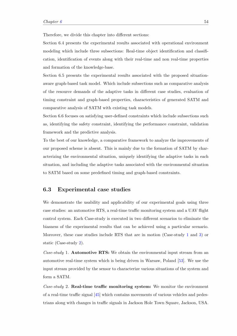
Chapter 6 54

Therefore, we divide this chapter into different sections:

Section 6.4 presents the experimental results associated with operational environment

modeling which include three subsections: Real-time object identification and classifi-

cation, identification of events along with their real-time and non real-time properties

and formation of the knowledge-base.

Section 6.5 presents the experimental results associated with the proposed situation-

aware graph-based task model. Which include subsections such as comparative analysis

of the resource demands of the adaptive tasks in different case studies, evaluation of

timing constraint and graph-based properties, characteristics of generated SATM and

comparative analysis of SATM with existing task models.

Section 6.6 focuses on satisfying user-defined constraints which include subsections such

as, identifying the safety constraint, identifying the performance constraint, validation

framework and the predictive analysis.

To the best of our knowledge, a comparative framework to analyze the improvements of

our proposed scheme is absent. This is mainly due to the formation of SATM by char-

acterizing the environmental situation, uniquely identifying the adaptive tasks in each

situation, and including the adaptive tasks associated with the environmental situation

to SATM based on some predefined timing and graph-based constraints.

6.3 Experimental case studies

We demonstrate the usability and applicability of our experimental goals using three

case studies: an automotive RTS, a real-time traffic monitoring system and a UAV flight

control system. Each Case-study is executed in two different scenarios to eliminate the

biasness of the experimental results that can be achieved using a particular scenario.

Moreover, these case studies include RTS that are in motion (Case-study 1 and 3) or

static (Case-study 2).

Case-study 1. Automotive RTS: We obtain the environmental input stream from an

automotive real-time system which is being driven in Warsaw, Poland [53]. We use the

input stream provided by the sensor to characterize various situations of the system and

form a SATM.

Case-study 2. Real-time traffic monitoring system: We monitor the environment

of a real-time traffic signal [45] which contains movements of various vehicles and pedes-

trians along with changes in traffic signals in Jackson Hole Town Square, Jackson, USA.

Chapter 6 55

The system interacts with various objects of its environment and generates a SATM

which allows the system to execute additional tasks at runtime.

Case-study 3. UAV flight control system: We also obtain the environmetal input

stream of the environment of an UAV which is running in Brigham City [54] (Scenario 1)

and New York city [55] (Scenario 2). The environment of the UAV contains movements

of various objects (such as people, car, and truck) as well as obstacles (like high rise

buildings, and trees) in its path.

6.4 Operational environment model

A dataset of an RTS can allow us to analyze the characteristics of system behavior along

with its users and the environment. Although many data collection approaches exist,

storing video stream is more useful as it provides sequential real-time information of the

system and visually represents the data so that we have a clear, straightforward and

precise understanding of the execution environment. Hence, we receive video stream as

input.

The object detector and classifier in the detection module of the operational environment

model views object detection in a video frame as a regression problem. Identification and

classification of the object from a video frame are complicated. Most of the early works

focus on identifying the object using feature extraction approaches which include Haar-

like features, Histogram of oriented gradients, Scale-invariant feature transform, Speeded

up robust feature and classifying using different machine learning algorithms like Support

vector machine [56], Random forest [57], and Artificial neural network [58]. However, the

deep neural network has gained much attention in recent days as it provides a significant

improvement over the early approaches in terms of detection and classification accuracy.

6.4.1 Real-time object identification and detection

To detect and classify objects from the video stream received from the camera, we use a

nine-layer convolutional neural network which is followed by two fully connected layers.

We divide each video frame into 10× 10 grid. The neural network detects an object by

predicting its appearance in multiple boxes. It also identifies the class probabilities for

each detected objects. We use the ImageNet dataset [59] to train our model offline, and

PASCAL VOC [60] to evaluate our detection scheme. Object detection and classification

using our scheme for the Automotive RTS (Case-study 1), Real-time traffic monitoring

Chapter 6 56

(a) Automotive RTS (b) Real-time traffic monitor-ing system

(c) UAV flight control system

Figure 6.1: Real-time object identification and classification using our approach

system (Case-study 2) and UAV flight control system (Case-study 3) are illustrated in

Figure 6.1.

6.4.2 Identification of events along with their real-time and non-real

time properties

Operational environment modeling includes analyzing the video stream and identify-

ing the events in different situations of RTS. We also analyze the detected events and

identify their real-time properties such as duration and periodicity and non real-time

properties such as location and speed. We use the periodic property of the events to

classify the events into periodic and aperiodic. The operational environment model char-

acterizes environmental situations in terms of events identified in different timestamps.

The statistics of the detected events in the two scenarios of Case-study 1, 2 and 3 are

presented in Table 6.1.

In Table 6.1, C denotes Case-study, and S denotes Scenario. For example, C1-S1 repre-

sents Case-study 1 - Scenario 1. For each scenario, for Case-study 1, 2, and 3, Table 6.1

illustrates the total number of identified events. Table 6.1 also shows the number of

basic and derived events in each scenario as well as compares the number of events in

terms of static and in motion. For Case-study 1 - scenario 1, we find 98.6% events are

basic, and 1.4% events are derived whereas for scenario two 98.02% events are basic.

For Case-study 2, the percentage of basic events are 83.64% and 84.02% in scenario 1

and 2. Whereas, for Case-study 2 the ratio of basic-derived events are (5.11 : 1) and

(5.26 : 1) in scenario 1 and 2 respectively.

Chapter 6 57

Table 6.1: Statistics of the detected events.

Events Basic - Derived Motion - Static

C1-S1 17234 16993-241 16765-469

C1-S2 9404 9223-181 9089-315

C2-S1 8113 6786-1327 6385-1728

C2-S2 9007 7568-1439 7114-1893

C3-S1 8221 5448-2733 6993-1228

C3-S2 9807 8068-1739 7614-2093

6.4.3 Formation of a knowledge-base

For each set of detected events, we use association rules to identify derived events which

are the result of basic events. We perform event reduction where the occurrence of each

event is recorded only once. For example, consider that E1 is a basic event, it can also

be used to form a derived event E8 which is a combination of E1 and E2. We ensure

that E1 is recorded only once. Therefore, for each time video frame is obtained, we store

each events id, timestamp, location, state, and speed. We form a knowledge-base which

takes significantly less memory consumption than raw video stream data.

The initial sizes of the video streams received from Case-study 1 are 11917513 kilobytes

(scenario 1), and 8550321 kilobytes (scenario 2), from Case-study 2 are 8691678 kilobytes

(scenario 1) and 9511215 kilobytes (scenario 2) and from Case-study 3 are 14319678

kilobytes (scenario 1) and 11815432 kilobytes (scenario 1). The produced knowledge-

base consumes significantly less memory in comparison to traditional video compression

techniques. The sizes of the created textual knowledge-base are 2262, 1576, 1577, 1679,

2821, and 1878 kilobytes memory respectively for Case-study 1, 2 and 3.

6.5 The proposed situation-aware graph-based task model

For each situation, we identify the adaptive tasks which are needed to be activated.

The adaptive tasks considered in this work for different Case-study are illustrated in

Table 6.2.

6.5.1 Comparative analysis of the resource demands of the adaptive

tasks in different case studies

For each Case-study, in each situation, we map the detected events into the adaptive

tasks defined in Table 6.2. Algorithm 5 evaluates the constraints associated with the

activated tasks and determines feasibility. For each situation, if the execution path

Chapter 6 58

0

50

100

150

200

250

300

350

400

450

Res

ourc

e de

man

d of

ada

ptiv

e ta

sks

0 1000 2000 3000 4000 5000 6000 7000

Time interval

(a) Case-study 1

0

50

100

150

200

250

300

350

400

450

500

Res

ourc

e de

man

d of

ada

ptiv

e ta

sks

0 1000 2000 3000 4000 5000 6000 7000

Time interval

(b) Case-study 2

0

20

40

60

80

100

120

140

160

180

Res

ourc

e de

man

d of

ada

ptiv

e ta

sks

0 1000 2000 3000 4000 5000 6000 7000

Time interval

(c) Case-study 3

Figure 6.2: Comparative analysis of resource demands in different case studies

Chapter 6 59

Table 6.2: List of adaptive tasks considered in this work in different case studies

Case-study 1 Case-study 3 Case-study 2

Turn right - 90 degree X + 30 degree Turn red light- on

Turn right - 60 degree X - 30 degree Turn red light- off

Turn right - 30 degrees Y + 30 degree Turn yellow light- on

Turn left - 90 degree Y - 30 degree Turn yellow light- off

Turn left - 60 degree Z + 30 degree Turn green light- on

Turn left - 30 degree Z - 30 degree Turn green light- off

Speed up Speed up

Speed down Speed down

Brake Brake

of the activated adaptive tasks is already included in the SATM, we avoid adding or

merging the tasks in SATM. However, if the adaptive tasks are absent in the SATM,

Algorithm 5 identifies the execution path and adds or merges them with existing SATM

offline. Figure 6.2 illustrates the resource demands associated with the adaptive tasks

identified in each situation for all three case studies.

6.5.2 Evaluation of timing constraint and graph-based properties

For each situation, the proposed RTS evaluates the identified adaptive tasks using a

number of constraints. It avoids including the adaptive tasks which violate the timing

and graph-based constraints to the SATM.

6.5.2.1 Comparison of scheduling overhead with vs. without timing evalu-

ation

We perform a comparison of the scheduling overhead (in nanoseconds) associated with

the adaptive tasks obtained in different situations for all three case studies considering

and without considering timing evaluations. With the introduction of the timing evalu-

ations at runtime, we experience reduced resource demands which can be translated to

decreased scheduling overhead in different situations because the proposed RTS avoids

including those tasks which do not satisfy the constraints. Figure 6.3 illustrates that

the scheduling overhead for the adaptive tasks are always either equal or low when we

consider timing evaluations.

Chapter 6 60

-600

-400

-200

0

200

400

600

Sch

edul

ing

Ove

rload

(na

nose

cond

s)

0 1000 2000 3000 4000 5000 6000 7000

Time interval

Without evaluationWith evaluation

(a) Case-study 1

-4000

-2000

0

2000

4000

6000

8000

10000

Sch

edul

ing

Ove

rload

(na

nose

cond

s)

0 1000 2000 3000 4000 5000 6000 7000

Time interval

Without evaluationWith evaluation

(b) Case-study 2

-3000

-2000

-1000

0

1000

2000

3000

4000

5000

6000

Sch

edul

ing

Ove

rload

(na

nose

cond

s)

0 1000 2000 3000 4000 5000 6000 7000

Time interval

Without evaluationWith evaluation

(c) Case-study 3

Figure 6.3: Comparative analysis of the scheduling overload using vs. without usingtiming evaluations

Chapter 6 61

6.5.2.2 Comparison of the probability of failure with vs. without timing

evaluation

Each adaptive task associated with an environmental event generated various external

components (objects). Different components have different failure rates. In this case,

we consider the causal failure probabilities associated with the components which are

generating the tasks. For the same data and the same system, we verify the tasks

associated with an event. Our system rejects the tasks associated with the event or

component whose failure probability is high. We determine the failure probability of the

system again, and Figure 6.4 illustrates the probability of system failure without and

considering the evaluations. Figure 6.4 demonstrates that the probability of failure is

much lower when the evaluations are performed (for Case-study 1, 2 and 3).

6.5.2.3 Comparison of self-adaptation time with vs. without timing evalu-

ation

For each situation, the system evaluates the identified adaptive tasks using a number

of timing TC and graph-based constraints GC. It avoids including the adaptive tasks

which violate the timing and the graph-based constraints to the SATM. We perform a

comparison of the resource demand(in nanoseconds) obtained at runtime for both case

studies using and without using TC and GC. With the introduction of the TC and GC at

runtime, Figure 6.5 presents a significant improvement in the resource demand because

the RTS avoids including those tasks which do not satisfy the timing and graph-based

constraints.

6.5.3 Comparative analysis of SATM with existing task models

For all the adaptive tasks obtained in different situations of Case study 1, 2 and 3, we

use existing multiframe task models such as GMF and NC - GMF and graph-based

task models such as RB, RRT, and NC - RRT and schedule them in a uniprocessor

environment. For each situation, for each task model, we identify the average execution

time of the adaptive tasks (average adaptation time). We also identify the overall average

response time where we consider both internal and adaptive tasks. An adaptive task

set exhibit adaptation failure if they can not satisfy the timing evaluations. For each

model, in each Case-study, we also identify adaptation failures.

Chapter 6 62

0 1000 2000 3000 4000 5000 6000 7000

Time intervals

0

0.01

0.02

0.03

0.04

0.05

0.06

0.07

Pro

babi

lity

of s

yste

m fa

ilure

Without evaluationWith evaluation

(a) Case-study 1

0 1000 2000 3000 4000 5000 6000 7000

Time intervals

0

0.01

0.02

0.03

0.04

0.05

0.06

0.07

Pro

babi

lity

of s

yste

m fa

ilure

Without evaluationWith evaluation

(b) Case-study 2

0 1000 2000 3000 4000 5000 6000 7000

Time intervals

0

0.005

0.01

0.015

0.02

0.025

0.03

0.035

0.04

0.045

0.05

Pro

babi

lity

of s

yste

m fa

ilure

Without evaluationWith evaluation

(c) Case-study 3

Figure 6.4: A comparison of probability of failure (with vs without evaluation)

Chapter 6 63

0 1000 2000 3000 4000 5000 6000 7000

Time interval

0

500

1000

1500

2000

2500

3000

3500

4000

4500

5000

Ada

ptat

ion

time

(nan

osec

onds

)

With evalutionWithout evalution

(a) Case-study 1

0 1000 2000 3000 4000 5000 6000 7000

Time interval

0

500

1000

1500

2000

2500

3000

3500

4000

4500

5000

Ada

ptat

ion

time

(nan

osec

onds

)

With evalutionWithout evalution

(b) Case-study 2

0 1000 2000 3000 4000 5000 6000 7000

Time interval

0

500

1000

1500

2000

2500

3000

3500

4000

4500

Ada

ptat

ion

time

(nan

osec

onds

)

With evalutionWithout evalution

(c) Case-study 3

Figure 6.5: Improvement of adaptation timing and graph-based evaluation.

Chapter 6 64

While identifying the adaptive tasks associated with a particular situation, the proposed

SATM efficiently maps events with tasks. For each event, we identify whether the task

associated with the event is already included in the SATM or not. If the task is already

present in SATM, we avoid including (and thereby executing) it in SATM. Hence, for

multiple events (which exhibit the same occurrence pattern), we add just one task.

Moreover, SATM also has a provision for merging the tasks with existing paths such

that the overall response time is lower. Hence, for a particular situation, the length

of the execution path of the adaptive tasks provided by SATM (adaptation time) is

significantly less in comparison to the existing task models.

We perform a comparison of scheduler complexity using and without using SATM. Fig-

ure 6.6(a), Figure 6.6(b), and Figure 6.6(c) represent a comparative analysis of the task

models which include GMF, NC-GMF, RB, RRT, and NC-RRT with the SATM. With

the introduction of the SATM, we see a significant improvement in average adaptation

time, average response time due to reduced length of the considered execution path of

the adaptive tasks. Also, execution paths which have reduced length are more likely to

satisfy time timing evaluations. Hence, in Figure 6.6, we also experience fewer adapta-

tion failures in all case studies. In this work, we consider the time interval δ as 2500

nanoseconds. Therefore, for each time interval, δ = 2500 is considered as the maximum

supply.

Lemma 1 and 2 imply that our system can handle overload situations because the length

of the execution path (even during merging with an existing path) never exceeds δ. Fig-

ure 6.2 also validates this statement because of the presence of SATM, the proposed RTS

ensures that the resource demand never exceeds 2500 nanoseconds (maximum supply) in

any time interval. Since the resource demand can exceed the supply 2500 nanoseconds,

the experimental results also show that the proposed SATM is feasible.

6.5.4 Characteristics of generated SATM

In this work, we use historical and current events from the situation-driven dataset to

characterize the runtime behavior of the RTS at different time intervals. For each time

interval, we identify the adaptive tasks that are needed to be executed due to the events

obtained from the environment. We determine the overload of the system based on the

set of available tasks which need to be executed. We also calculate the response time

Chapter 6 65

GMF NC-GMF RB RRT NC - RRT SATM0

500

1000

1500

2000

2500

3000

Avg Adaptation demandAvg overall responsetimeTotal adaptation failure

(a) Case-study 1

GMF NC-GMF RB RRT NC - RRT SATM0

500

1000

1500

2000

2500

3000

3500

4000

4500

5000

Avg Adaptation demandAvg overall responsetimeTotal adaptation failure

(b) Case-study 2

GMF NC-GMF RB RRT NC - RRT SATM0

500

1000

1500

2000

2500

3000

3500

4000

4500

5000

Avg Adaptation demandAvg overall responsetimeTotal adaptation failure

(c) Case-study 3

Figure 6.6: Performance comparison of different task models with SATM

Chapter 6 66

and execute available tasks such that a particular task is not executed more than once.

Hence, unnecessary execution of a task more than once is removed.

Table 6.3: Characteristics of the SATM.

Total Events Number of vertices Number of edges

C1-S1 17234 9 44

C1-S2 9404 9 43

C2-S1 8113 9 56

C2-S2 9007 9 68

C3-S1 8221 6 36

C3-S2 9807 6 36

We use the SATM to execute the tasks at runtime if they are already included in the

SATM. Otherwise, we store their information and further evaluate the constraints and

update the SATM (offline), if they satisfy the constraints.

Table 6.3 shows that for Case-study 1 - scenario 1, the generated SATM contains nine

verities (tasks) and 44 edges. Whereas, for scenario 2, the SATM consists of nine vertices

and 43 edges. For Case-study 2, the constructed SATM has nine vertices as well as 56

edges for scenario 1 and nine vertices along with 36 edges for scenario 2. The reason

behind the generated SATM containing a smaller number of vertices is due to the efficient

mapping of multiple events to a particular task and merging the tasks in an existing

execution path. In the future situations, we obtain same/similar (events which have

same occurrence pattern) events and thereby, similar situations for a number of times

at runtime. Table 6.3 illustrates that the proposed can represent the execution behavior

of the adaptive tasks of the RTS in smaller memory.

6.5.5 Comparative analysis of the adaptation time (SATM vs. existing

task models)

In this work, for a particular situation, the RTS can use a pre-determined execution

path, if the situation has appeared before. Figure 6.7 illustrates that cases in which the

tasks associated with the identified events in a particular situation are already present

in the SATM, we experience a significant reduction in adaptation time for identification

of the execution order of the adaptive tasks. The reason for such reduction is that

the execution of a number of activities which include evaluation of the constraints,

identifying the execution orders, finding vertices, merging the vertices associated with

the adaptations with existing execution paths does not take place in these cases, because

the vertices associated with the situation is already included in the SATM.

Chapter 6 67

0 1000 2000 3000 4000 5000 6000 7000

Time interval

1000

2000

3000

4000

5000

6000

7000

8000

9000

Ada

ptat

ion

time

(nan

osec

onds

)

NC-GMFSATM

(a) Case-study 1

0 1000 2000 3000 4000 5000 6000 7000

Time interval

1000

1500

2000

2500

3000

3500

4000

4500

5000

5500

Ada

ptat

ion

time

(nan

osec

onds

)

RBSATM

(b) Case-study 2

0 1000 2000 3000 4000 5000 6000 7000

Time interval

0

5000

10000

15000

Ada

ptat

ion

time

(nan

osec

onds

)

NC-RRTSATM

(c) Case-study 3

Figure 6.7: Improvement of adaptation time due to SATM at runtime.

Chapter 6 68

6.6 Satisfying user-defined constraints

6.6.1 Identifying the safety constraint

We use fault tree to perform deductive failure analysis of the RTS. Fault tree analysis also

allows us to have meaningful insights on identifying key system elements, environmental

events which can cause a failure and investigates many ways a fault can occur. Our

system performs both component and event-based safety analysis. For component-based

analysis, we use safety integrity level defining failure probability of different components

of the system in various timestamps of video frame arrival. The fault tree deduces failure

likelihood of the undesired top event (which in our case is an accident and it can be due

to component failure or collision between two events that are in motion).

In each timestamp, we identify events that might lead to the top events and their asso-

ciated probabilities. But this is the result obtained from only from the straightforward

events (basic) which are already detected from the video streams. However, the system

can experience some uncertain events which might go unnoticed in video streams. We

use the Bayesian formula to determine the probability of the uncertain events from the

detected events. Bayesian analysis enables us to take uncertainties related to the sys-

tem environment into account and allows incorporating prior information. Figure 6.8

presents the probability of failure of the derived event, the probability of failure without

considering the derived event and probability of failure of the system considering the

derived event (safety constraint) for Case-study 1. Similarly, we identify the probability

of failure for situation-aware RTS for Case-study 2 and Case-study 3.

6.6.2 Identifying the performance constraint

We use different time windows for identifying the performance of the RTS. For each

time window, we identify the number of events processed. The maximum capacity of

the system is calculated by comparing the maximum number of events detected in all

the different time windows. Our system calculates maximum load and selects the time

window which contains the maximum number of events being processed. For each time

window, we identify the usage as the cumulative overhead of the time required for pro-

cessing the events. Our performance analysis takes the entire time interval (starting from

one to video frame arrival time) into account. As the system is introduced with more

events in different scenarios, the system delivers a more accurate reflection of its capacity

Chapter 6 69

0 500 1000 1500 2000 2500 3000 3500

Identified events in different timestamps

0

0.1

0.2

0.3

0.4

0.5

0.6

0.7

0.8

0.9

1

Pro

babi

lity

of fa

ilure

of t

he d

eriv

ed e

vent

s 10-3

Probablity of failureSIL 4Maximum probablity of failure

(a) Probability of failure of derived events

0 500 1000 1500 2000 2500 3000 3500

Identified events in different timestamps

0

0.5

1

1.5

2

2.5

3

Pro

babi

lity

of fa

ilure

of R

TS

with

out i

nclu

ding

der

ived

eve

nts

10-3

Probablity of failureSIL 4Maximum probablity of failure

(b) Probability of failure without including derived events

0 500 1000 1500 2000 2500 3000 3500

Identified events in different timestamps

0

0.5

1

1.5

2

2.5

3

3.5

4

Pro

babi

lity

of fa

ilure

of R

TS

incl

udin

g de

rived

eve

nts

10-3

Probablity of failureSIL 4Maximum probablity of failure

(c) Probability of failure of the situation-aware RTS

Figure 6.8: Probability of failure of the situation-aware RTS in different timestampsfor Case-study 1

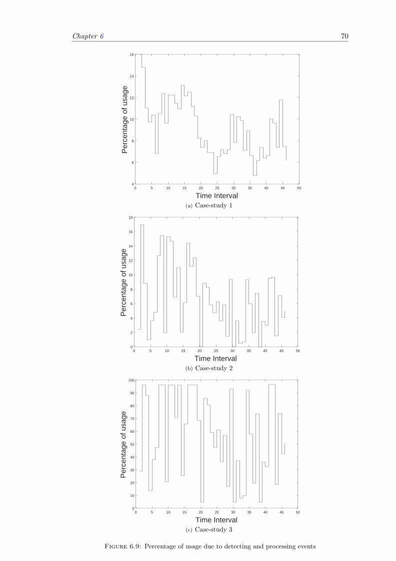
Chapter 6 70

0 5 10 15 20 25 30 35 40 45 50

Time Interval

4

6

8

10

12

14

16

Per

cent

age

of u

sage

(a) Case-study 1

0 5 10 15 20 25 30 35 40 45 50

Time Interval

0

2

4

6

8

10

12

14

16

18

Per

cent

age

of u

sage

(b) Case-study 2

0 5 10 15 20 25 30 35 40 45 50

Time Interval

0

10

20

30

40

50

60

70

80

90

100

Per

cent

age

of u

sage

(c) Case-study 3

Figure 6.9: Percentage of usage due to detecting and processing events

Chapter 6 71

usage. We can use performance analysis to provide some constructive feedback and sug-

gestions which can help the system to improve its efficiency. In our experiment, a time

interval of 55 milliseconds was selected as it contains a maximum of 183 detected events.

We determine the percentage of usage for the selected time window. Figure 6.9(a), Fig-

ure 6.9(b), and Figure 6.9(c) illustrates the capacity usage of the system for Case-study

1, 2 and 3 respectively.

6.6.3 Validation framework

The RTS system presented in our work has two modes of operations: safety, and per-

formance. For each time the validation framework calculates the probability of failure

of the system using fault tree analysis. The validation framework defines a threshold

value called SV which is the total probability of failure to determine whether a system

is safe or not and determine the expected mode. The validation framework uses a state

machine to demonstrate the system behavior where the system modes are represented

by states and two events namely up and down are used for transition between the modes.

6.6.3.1 Comparative analysis of modes changes (with vs. without validation

framework)

Our system satisfies the user-defined constraints by changing its operating mode at

runtime. Situations in which the probability of failure is high, it assures reliability by

changing the operating mode to Safety (from performance). Figure 6.4 demonstrates

that the probability of failure is much lower when the validation framework is used.

This is because when the validation framework is used the system changes its operating

mode to safety when the probability of failure is higher than TH = .01 and satisfies

user-defined constraints.

With the arrival of a new situation, in each time interval, we determine the expected

mode. If the probability of failure is more than a predefined threshold value (which

is .01), our expected mode safety. The system changes its operating mode at differ-

ent times so that it can avoid any failures at runtime. Figure 6.10(a), Figure 6.10(b)

and Figure 6.10(c) present changes in the operating mode at different time intervals

(considering and without considering validation framework) for Case-study 1, 2 and 3

respectively.

Chapter 6 72

0 500 1000 1500 2000 2500 3000 3500

Time interval

Safety mode before

Performance mode before

Safety mode after

Performance mode after

(a) Case-study 1

0 500 1000 1500 2000 2500 3000 3500

Time interval

Safety mode before

Performance mode before

Safety mode after

Performance mode after

Mod

es o

f ope

ratio

n

(b) Case-study 2

0 500 1000 1500 2000 2500 3000 3500

Time interval

Safety mode before

Performance mode before

Safety mode after

Performance mode after

Mod

es o

f ope

ratio

n

(c) Case-study 3

Figure 6.10: Changes of modes of operation in different time interval

Chapter 6 73

Old Safety New Safety Old Performance New Performance

Modes of operation

0

500

1000

1500

2000

2500

3000

3500

Num

ber

of o

ccur

ance

s

Mode changes afterMode changes before

(a) Case-study 1

Old Safety New Performance Old Performance New Safety

Modes of operation

0

500

1000

1500

2000

2500

3000

3500

Num

ber

of o

ccur

ance

s

1-1-15Mode changes afterMode changes before

(b) Case-study 2

Old Safety Old Performance New Safety New Performance

Modes of operation

0

500

1000

1500

2000

2500

3000

3500

Num

ber

of o

ccur

ance

s

Mode changes afterMode changes before

(c) Case-study 3

Figure 6.11: A comparison of mode changes with vs. without validation framework

Chapter 6 74

We also present the number of occurrences of various operating modes of the system.

Figure 6.10(a), Figure 6.10(b) and Figure 6.10(c) demonstrates mode switching from

safety to performance (and vice versa) as well as the total duration (time interval)

in the destination mode. The system operates in performance mode in most of the

time intervals to satisfy the performance (usage) requirements. It also switches from the

performance to the safety mode when the probability of failure is high. This experimental

result illustrates that the RTS meets our user-defined constraints satisfaction goal at

runtime because the system can use multiple modes of operation at runtime to guarantee

performance and safety requirements.

(a) Randomized detection of collision (b) Detection of collision using our ap-proach

Figure 6.12: Prediction of collision using Motion modeling

Figure 6.11(a), Figure 6.11(b), and Figure 6.11(c) presents a comparative view of the

occurrences of different modes in various time interval for Case-study 1, 2 and 3 respec-

tively. The old result (mode changes) is obtained without considering the validation

framework. Figure 6.11(a), Figure 6.11(b), and Figure 6.11(c) presents that, with the

introduction of validation framework, the RTS operate more (in terms of time intervals)

in safety mode and thereby satisfies the user-defined safety and performance constraints.

6.6.4 Predictive analysis

In this thesis, we perform trajectory predictions by performing real-time tracking of the

identified events associated with objects. We keep track of all the events with their

location along with an average change in their position. For each event in motion, our

system determines average the changes in x and y coordinate of the objects. We use

current location of the object along with its average changes and use LSTM to perform

Chapter 7 75

motion modeling which predicts the future locations of all the events and identifies

whether collision takes place within any two or more events.

Although some existing approaches prevail that detects collisions using various physical

models. Our prediction model is adaptive and can address changing situations as it

updates the location information each time a new frame arrives and recalculates the

possible future locations. Our trajectory prediction framework is tested in different video

streams, and it was successfully able to predict collisions. An illustration of comparison

for detection of collision using our framework with a randomized collision prediction

approach is provided in Figure 6.12.

Chapter 7

Conclusion

With the growing number of real-time systems and extensive integration of real-time

systems in different Cyber-Physical Systems, Smart Cities and Internet of Things, users

today expect systems to operate whenever and wherever they want. Systems are now

becoming highly interactive, consist of several operating modes and must be able to

execute in a changing environment. Designing, configuring, and assuring the functional

and runtime behavior of such systems are very challenging. To cope with the challenge,

we present the design of a situation-aware real-time system which can satisfy user-defined

constraints.

We present a situation-aware graph-based task model which allows an RTS to accom-

modate the execution of adaptive tasks in different situations. To identify the adaptive

tasks that need to be executed in a particular situation, we monitor the environment of

an RTS and translate the events identified in a particular situation into a set of adap-

tive tasks. We ensure schedulability by defining a number of constraints and evaluating

the adaptive tasks using the constraints. We avoid including the tasks to the tasks

model which violate the constraints. Such evaluation allows the RTS to reduce resource

demand of the adaptive tasks at runtime. Formation of SATM includes mapping the

adaptive tasks as vertices and execution order between each pair of tasks as an edge.

If the vertices satisfy the constraints, the proposed SATM finds their execution path

and merges the new execution path with the existing SATM. SATM also facilitates a

reduced adaptation time in different situations. Formation of SATM is performed of-

fline. However, the SATM can handle a particular situation at runtime, if the vertices

identified from the situation that are already included in the SATM.

The presented design of the situation-aware real-time system contains non-adaptive and

76

Chapter 7 77

adaptive execution models. In non-adaptive execution model, the RTS only executes

internal task set defined by current mode using the EDF scheduling algorithm. In

adaptive execution model, the RTS monitors its environment, identifies the real-world

occurrences as events and determines their real-time (such as duration, and periodicity)

and non real-time (such as location, and speed) properties. We determine the association

relationships involved among the events through performing association rule learning.

We create a knowledge-base (offline) which stores the historical event information from

the captured situations. The knowledge-base allows fast information retrieval in reduced

memory and facilitates the formation of SATM.

We use the knowledge-base to determine the safety constraints in different environmen-

tal situations. Identification of the safety constraint involves performing a fault-tree

analysis and determining the probability of failure of the RTS in each environmental

situation. We also identify the performance constraint for each environmental situation

by analyzing the capacity along with the usage of the RTS at different situation arrival

time interval.

We present a validation framework, which uses the probability of failure identified in a

particular situation to determine whether the RTS is operating in the expected mode or

not. The validation framework also provides reliability by defining a verification action

which allows the RTS to change its operating modes at runtime. The RTS can satisfy

the user-defined constraints and avoid failure in adverse environmental situations by

switching its operating mode at runtime. For example, the RTS can satisfy the safety

constraint by operating in the safety mode when the probability of failure is high.

To the best of our knowledge, a framework for designing a situation-aware RTS that

analyzes environmental input stream, identifies various events and extracting numerous

real-time and non real-time properties among the events, discovers associations among

the events, produces a knowledge-base, changes the modes of operation to ensure the

user-defined constraints of the system at runtime, creates the SATM by characterizing

the environmental situations, uniquely identifies the adaptive tasks in each situation,

and includes the adaptive tasks associated with the environmental situation to SATM

based on some predefined timing constraints and graph-based properties is absent.

The future work of this thesis includes enabling communications among the considered

case studies. Moreover, we also aim to present additional user-defined constraints other

than safety and performance. Another future work is to allow the system to operate in

Chapter 7 78

additional operating modes (other than safety and performance) and implementing ex-

isting mode change protocols such as Maximum Period Offset, Minimum Offset without

periodicity, Minimum Offset with periodicity, Asynchronous with periodicity and Asyn-

chronous without periodicity for mode switching. Moreover, we also aim to formulate

a task model which can characterize the mode transitions of all the considered modes.

Moreover, we aim to execute the adaptive tasks using additional task models (other than

GMF, NC-GMF, RB, RRT, and NC-RRT).

Modern RTS requires computing infrastructure which allows low-latency network con-

nections with deterministic transmission time with other systems as well as the Internet.

Fog computing has gained much attention in recent days where various analytics can

be performed at end devices such as access points or set-top-boxes [61] which can be

considered as fog nodes. An RTS embedded within fog architecture can allow processing

to be performed to close as possible to the system. For example, consider a scenario

where we have multiple vehicles running on a road (each having analytics endpoints),

can send and process information in the fog node. Such RTS design can provide reduced

network overhead and processing time as well as more security in comparison to storing

and processing data using cloud computing.

We also aim to present a Fog-based analytics framework from mining the environmen-

tal input stream of the situation-aware system where we consider that the RTS has an

analytics endpoint (fog node) which allows the system to communicate nearby trans-

portation systems. For each situation, our goal is to send the events detected in a

particular situation to the fog node and present a fog computing-based analytics frame-

work which determines the user-defined constraints associated with each situation in the

fog node.

Appendix A

An Appendix

Different symbols used in this paper can be listed as:

• µ = {µ1, µ2}, is the set of RTS modes of operation.

• µcurrent is the current operating mode such that µcurrent ∈ µ.

• µexpected is the expected operating mode such that µexpected ∈ µ.

• τout = {τout1 , τout2 , . . . , τoutr} is a set of r adaptive real-time tasks such that r ∈ N+.

• τMCR is the task which triggers a mode change request. item τi is an active task

defined as τi = (αi,Ci,Di), (such that i ∈ N+.) where,

– αi is the arrival time,

– Ci is the worst-case execution time demand, and

– Di is the relative deadline of τi.

• τin = {τin1 , τin2 , . . . , τinq} is a set of q active internal real-time tasks with q ∈ N+.

• Pi is the period of internal task τini ∈ τin.

• dbfτin(δ) is the demand-bound function for time interval δ and the set of tasks τin.

• rfτout(δ) is the request function for time interval δ and the set of tasks τout.

• Ob is the bth Object such that b ∈ N+.

• Ec denotes cth Event such that c ∈ N+.

• AR is the rule set defining association rules among the events.

79

Chapter 7 80

• Ebasic is the set of basic events.

• Ederived is the set of derived events.

• Sk = {E1,E2, . . . ,Ed} is the Situation identified at time tk such that k, d ∈ N+.

• F = {f1, f2, . . . , fn} is the set of n video frames taken at a time interval δ such that

n, δ ∈ N+.

• ED = (x1, x2, . . . , xu) is a temporal vector which stores event information.

• KB is the generated knowledge-base.

• G(Sk) = (V,H) is the situation aware task graph where,

1. V is the set of vertices.

2. H is the set of directed edges.

• θ(τin) is the worst-case estimated duration for the internal tasks.

• Tavailable is the available free time slots after scheduling the internal tasks in δ.

• TC1(vi),TC2(vi, vi+1),TC3(vi),TC4(vi), and TC are the timing constraints.

• π(Sk) is the execution path associated with Sk.

• Length(π(Sk)) is the length of the execution path π(Sk) in terms of worst-case

execution time.

• dist(vi, vj) is the minimum distance of the vertex from vi ∈ V to vj ∈ V.

• diam(G) is the maximum distance between the two vertices (in terms of execution

time) of G.

• GC1,GC2,GC3, and GC are the graph-based constraints.

• SA1 is the non adaptive scheduling algorithm such that SA1 = EDF.

• SA2 is the adaptive scheduling algorithm such that SA2 : {τin ∪ (τout ⊆ G)} → Pr.

Bibliography

[1] Giorgio C Buttazzo. Hard real-time computing systems: predictable scheduling al-

gorithms and applications, volume 24. Springer Science & Business Media, 2011.

[2] Martin Stigge and Wang Yi. Graph-based models for real-time workload: a survey.

Real-Time Systems, 51(5):602–636, 2015.

[3] Sanjoy K Baruah, Aloysius K Mok, and Louis E Rosier. Preemptively scheduling

hard-real-time sporadic tasks on one processor. In Real-Time Systems Symposium,

1990. Proceedings., 11th, pages 182–190. IEEE, 1990.

[4] Nan Guan, Wang Yi, Zonghua Gu, Qingxu Deng, and Ge Yu. New schedulability

test conditions for non-preemptive scheduling on multiprocessor platforms. In 2008

Real-Time Systems Symposium, pages 137–146. IEEE, 2008.

[5] Jia Xu and David Lorge Parnas. Priority scheduling versus pre-run-time scheduling.

Real-Time Systems, 18(1):7–23, 2000.

[6] Mohammad I Daoud and Nawwaf Kharma. A high performance algorithm for static

task scheduling in heterogeneous distributed computing systems. Journal of Parallel

and distributed computing, 68(4):399–409, 2008.

[7] Chung Laung Liu and James W Layland. Scheduling algorithms for multiprogram-

ming in a hard-real-time environment. Journal of the ACM (JACM), 20(1):46–61,

1973.

[8] Jorge Real and Alfons Crespo. Mode change protocols for real-time systems: A

survey and a new proposal. Real-time systems, 26(2):161–197, 2004.

[9] Alan Burns. System mode changes-general and criticality-based. In Proc. of 2nd

Workshop on Mixed Criticality Systems (WMC), pages 3–8, 2014.

81

Bibliography 82

[10] Gabriel Leen and Donal Heffernan. Expanding automotive electronic systems. Com-

puter, 35(1):88–93, 2002.

[11] Pavla Pecherkova and Ivan Nagy. Analysis of discrete data from traffic accidents.

In Smart City Symposium Prague (SCSP), 2017, pages 1–4. IEEE, 2017.

[12] Christian Krupitzer, Felix Maximilian Roth, Sebastian VanSyckel, Gregor Schiele,

and Christian Becker. A survey on engineering approaches for self-adaptive systems.

Pervasive and Mobile Computing, 17:184–206, 2015.

[13] Betty HC Cheng, Kerstin I Eder, Martin Gogolla, Lars Grunske, Marin Litoiu,

Hausi A Muller, Patrizio Pelliccione, Anna Perini, Nauman A Qureshi, Bernhard

Rumpe, et al. Using models at runtime to address assurance for self-adaptive

systems. In Models@ run. time, pages 101–136. Springer, 2014.

[14] Sanjoy Baruah, Deji Chen, Sergey Gorinsky, and Aloysius Mok. Generalized mul-

tiframe tasks. Real-Time Systems, 17(1):5–22, 1999.

[15] Noel Tchidjo Moyo, Eric Nicollet, Frederic Lafaye, and Christophe Moy. On schedu-

lability analysis of non-cyclic generalized multiframe tasks. In Real-Time Systems

(ECRTS), 2010 22nd Euromicro Conference on, pages 271–278. IEEE, 2010.

[16] Sanjoy K Baruah. Feasibility analysis of recurring branching tasks. In Real-Time

Systems, 1998. Proceedings. 10th Euromicro Workshop on, pages 138–145. IEEE,

1998.

[17] Sanjoy K Baruah. Dynamic-and static-priority scheduling of recurring real-time

tasks. Real-Time Systems, 24(1):93–128, 2003.

[18] Sanjoy Baruah. The non-cyclic recurring real-time task model. In 2010 31st IEEE

Real-Time Systems Symposium, pages 173–182. IEEE, 2010.

[19] Sanjoy K Baruah. A general model for recurring real-time tasks. In Real-Time Sys-

tems Symposium, 1998. Proceedings. The 19th IEEE, pages 114–122. IEEE, 1998.

[20] Ragunathan Raj Rajkumar, Insup Lee, Lui Sha, and John Stankovic. Cyber-

physical systems: the next computing revolution. In Proceedings of the 47th Design

Automation Conference, pages 731–736. ACM, 2010.

Bibliography 83

[21] Aloysius K Mok and Deji Chen. A multiframe model for real-time tasks. IEEE

transactions on Software Engineering, 23(10):635–645, 1997.

[22] Xiangyang Xue, Wei Zhang, Yue-Fei Guo, Hong Lu, Yuejie Zhang, Zichen Sun,

Yingbin Zheng, Shile Zhang, Hong Liu, Yuanzheng Song, et al. Fudan university

at trecvid 2007. In TRECVID, 2008.

[23] Md Haris Uddin Sharif, Sahin Uyaver, and Md Haidar Sharif. Ordinary video events

detection. In CompIMAGE, pages 19–24, 2012.

[24] Xingquan Zhu, Xindong Wu, Ahmed K Elmagarmid, Zhe Feng, and Lide Wu.

Video data mining: Semantic indexing and event detection from the association

perspective. IEEE Transactions on Knowledge and Data engineering, 17(5):665–

677, 2005.

[25] Amit Adam, Ehud Rivlin, Ilan Shimshoni, and Daviv Reinitz. Robust real-time

unusual event detection using multiple fixed-location monitors. IEEE transactions

on pattern analysis and machine intelligence, 30(3):555–560, 2008.

[26] Eduardo Peixoto, Tamer Shanableh, and Ebroul Izquierdo. H. 264/avc to hevc video

transcoder based on dynamic thresholding and content modeling. IEEE Transac-

tions on Circuits and Systems for Video Technology, 24(1):99–112, 2014.

[27] Shijun Sun, Shankar Regunathan, Chengjie Tu, and Chih-Lung Lin. Conversion

operations in scalable video encoding and decoding, February 14 2017. US Patent

9,571,856.

[28] Xuemin Chen and Jason Demas. Artifact-free displaying of mpeg-2 video in the

progressive-refresh mode, May 2 2017. US Patent 9,641,858.

[29] Rajeev Alur and David L Dill. A theory of timed automata. Theoretical computer

science, 126(2):183–235, 1994.

[30] Johan Bengtsson and Wang Yi. Timed automata: Semantics, algorithms and tools.

Lecture Notes in Computer Science, 3098:87–124, 2004.

[31] Bernard Berthomieu and Michel Diaz. Modeling and verification of time dependent

systems using time petri nets. IEEE transactions on software engineering, 17(3):

259–273, 1991.

Bibliography 84

[32] Razieh Behjati, Hamideh Sabouri, Niloofar Razavi, and Marjan Sirjani. An effective

approach for model checking systemc designs. In Application of Concurrency to

System Design, ACSD 2008, pages 56–61. IEEE, 2008.

[33] Stewart Worrall, David Orchansky, Favio Masson, and Eduardo Nebot. Improv-

ing vehicle safety using context based detection of risk. In Intelligent Transporta-

tion Systems (ITSC), 2010 13th International IEEE Conference on, pages 379–385.

IEEE, 2010.

[34] Mattias Brannstrom, Erik Coelingh, and Jonas Sjoberg. Model-based threat as-

sessment for avoiding arbitrary vehicle collisions. IEEE Transactions on Intelligent

Transportation Systems, 11(3):658–669, 2010.

[35] M Hecht, D Buettner, and J Hellrung. Risk assessment of real time digital control

systems. In Reliability and Maintainability Symposium, 2006. RAMS’06. Annual,

pages 409–415. IEEE, 2006.

[36] Andre Arnes, Karin Sallhammar, Kjetil Haslum, Tønnes Brekne, Marie Moe, and

Svein Knapskog. Real-time risk assessment with network sensors and intrusion

detection systems. Computational Intelligence and Security, pages 388–397, 2005.

[37] Shi Jianjun, Wu Xu, Guan Jizhen, and Chen Yangzhou. The analysis of traffic

control cyber-physical systems. Procedia-Social and Behavioral Sciences, 96:2487–

2496, 2013.

[38] Cu D Nguyen, Simon Miles, Anna Perini, Paolo Tonella, Mark Harman, and Michael

Luck. Evolutionary testing of autonomous software agents. Autonomous Agents and

Multi-Agent Systems, 25(2):260–283, 2012.

[39] Nauman A Qureshi, Ivan J Jureta, and Anna Perini. Requirements engineering

for self-adaptive systems: Core ontology and problem statement. In International

Conference on Advanced Information Systems Engineering, pages 33–47. Springer,

2011.

[40] Nauman A Qureshi, Sotirios Liaskos, and Anna Perini. Reasoning about adaptive

requirements for self-adaptive systems at runtime. In Requirements@ Run. Time

(RE@ RunTime), 2011 2nd International Workshop on, pages 16–22. IEEE, 2011.

Bibliography 85

[41] Nauman A Qureshi and Anna Perini. Requirements engineering for adaptive service

based applications. In Requirements Engineering Conference (RE), 2010 18th IEEE

International, pages 108–111. IEEE, 2010.

[42] Basil Becker, Dirk Beyer, Holger Giese, Florian Klein, and Daniela Schilling. Sym-

bolic invariant verification for systems with dynamic structural adaptation. In Pro-

ceedings of the 28th international conference on Software engineering, pages 72–81.

ACM, 2006.

[43] Holger Giese, Stephan Hildebrandt, and Leen Lambers. Bridging the gap between

formal semantics and implementation of triple graph grammars. Software & Systems

Modeling, 13(1):273–299, 2014.

[44] Antonio Bucchiarone, Patrizio Pelliccione, Charlie Vattani, and Olga Runge. Self-

repairing systems modeling and verification using agg. In Software Architecture,

2009 & European Conference on Software Architecture. WICSA/ECSA 2009. Joint

Working IEEE/IFIP Conference on, pages 181–190. IEEE, 2009.

[45] Nayreet Islam and Akramul Azim. Carts: Constraint-based analytics from real-

time system monitoring. In Systems, Man, and Cybernetics (SMC), 2017 IEEE

International Conference on, pages 2164–2169. IEEE, 2017.

[46] John C Knight. Safety critical systems: challenges and directions. In Software

Engineering, 2002. ICSE 2002. Proceedings of the 24rd International Conference

on, pages 547–550. IEEE, 2002.

[47] Donal Heffernan, Ciaran MacNamee, and Padraig Fogarty. Runtime verification

monitoring for automotive embedded systems using the iso 26262 functional safety

standard as a guide for the definition of the monitored properties. IET Software, 8

(5):193–203, 2014.

[48] Cesare Alippi. Intelligence for embedded systems. Springer, 2014.

[49] Martin Stigge, Pontus Ekberg, Nan Guan, and Wang Yi. The digraph real-time

task model. In Real-Time and Embedded Technology and Applications Symposium

(RTAS), 2011 17th IEEE, pages 71–80. IEEE, 2011.

[50] Mark Charlwood, Shane Turner, and Nicola Worsell. A methodology for the assign-

ment of safety integrity levels (SILs) to safety-related control functions implemented

Bibliography 86

by safety-related electrical, electronic and programmable electronic control systems

of machines. HSE Books, 2004.

[51] Felix A Gers and E Schmidhuber. Lstm recurrent networks learn simple context-

free and context-sensitive languages. IEEE Transactions on Neural Networks, 12

(6):1333–1340, 2001.

[52] Christopher Olah. Understanding lstm networks. 2015. URL http://colah. github.

io/posts/2015-08-Understanding-LSTMs/img/LSTM3-chain. png, 2015.

[53] Karol Majek. Self driving car in warsaw, poland, 2017. URL https://drive.

google.com/file/d/0B_6iW8KaJFXOQmhaWU56dlBDY28/view.

[54] Box Elder 1963. Drone video of brigham city main street, 2018. URL https:

//www.youtube.com/channel/UCzntneOCzNs7yMzthOtGVFg.

[55] Jeff Tibbitts Bob Strobel and Lincoln Ramsey. Jackson hole town square-live

streaming, 2017. URL http://www.seejh.com/live?ref=sjhyt.

[56] Olivier Chapelle, Patrick Haffner, and Vladimir N Vapnik. Support vector machines

for histogram-based image classification. IEEE transactions on Neural Networks,

10(5):1055–1064, 1999.

[57] Anna Bosch, Andrew Zisserman, and Xavier Munoz. Image classification using

random forests and ferns. In Computer Vision, 2007. ICCV 2007. IEEE 11th

International Conference on, pages 1–8. IEEE, 2007.

[58] Michael Egmont-Petersen, Dick de Ridder, and Heinz Handels. Image processing

with neural networksa review. Pattern recognition, 35(10):2279–2301, 2002.

[59] Jia Deng, Wei Dong, Richard Socher, Li-Jia Li, Kai Li, and Li Fei-Fei. Imagenet:

A large-scale hierarchical image database. In Computer Vision and Pattern Recog-

nition, 2009. CVPR 2009. IEEE Conference on, pages 248–255. Ieee, 2009.

[60] Mark Everingham, Luc Van Gool, Christopher KI Williams, John Winn, and An-

drew Zisserman. The pascal visual object classes (voc) challenge. International

journal of computer vision, 88(2):303–338, 2010.

[61] Flavio Bonomi, Rodolfo Milito, Jiang Zhu, and Sateesh Addepalli. Fog computing

and its role in the internet of things. In Proceedings of the first edition of the MCC

workshop on Mobile cloud computing, pages 13–16. ACM, 2012.