Embed Size (px)
Citation preview

1
Design and Simulation of Micro-Power System of Renewables
Charles Kim, Ph.D.
Howard University, Washington, DC USA
• Citation: Charles Kim, “Lecture notes on Design and Simulation of Micro-Power Systems of Renewables”, 2013. Washington, DC.
Available at www.mwftr.com
• Note: This lecture note is a compilation of a 5-day lecture given at the Korean University of Technology Education in January 2013.
2
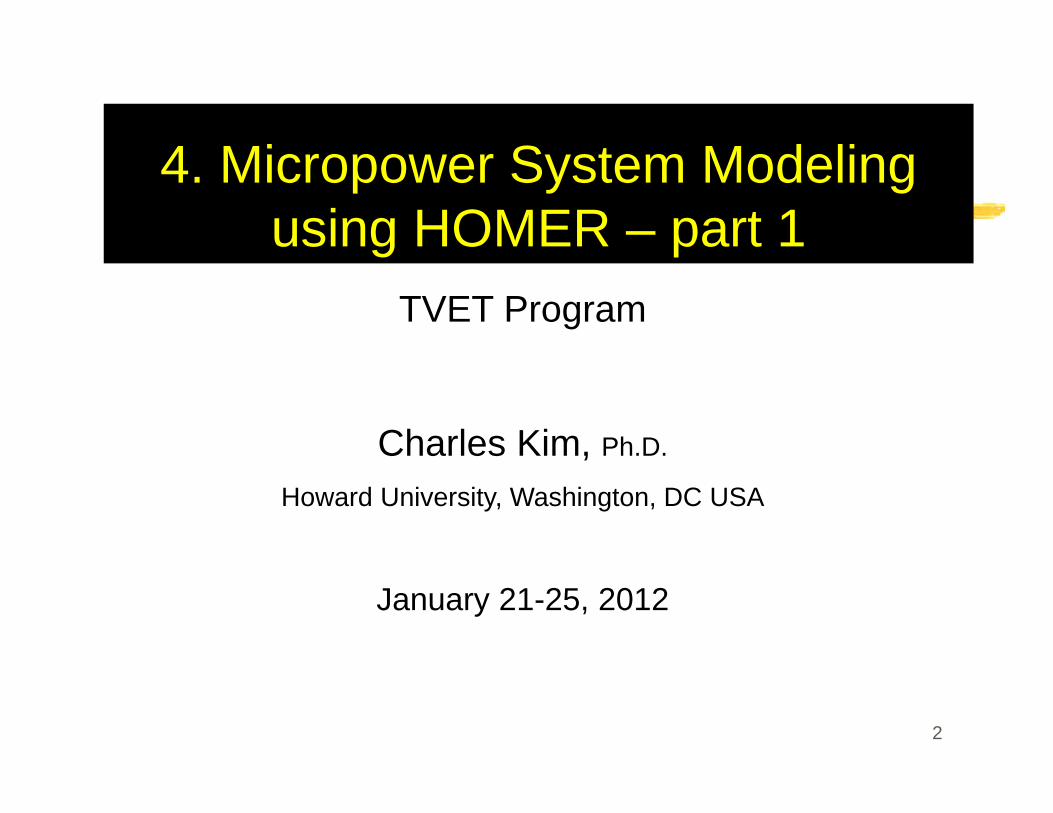
4. Micropower System Modeling using HOMER – part 1
TVET Program
Charles Kim, Ph.D.
Howard University, Washington, DC USA
January 21-25, 2012
3
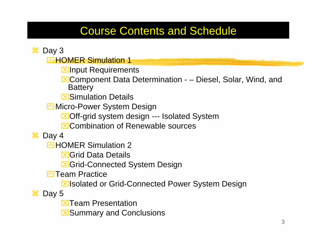
Course Contents and Schedule Day 3
HOMER Simulation 1⌧Input Requirements ⌧Component Data Determination - – Diesel, Solar, Wind, and
Battery⌧Simulation Details
Micro-Power System Design⌧Off-grid system design --- Isolated System⌧Combination of Renewable sources
Day 4HOMER Simulation 2⌧Grid Data Details⌧Grid-Connected System Design
Team Practice⌧Isolated or Grid-Connected Power System Design
Day 5⌧Team Presentation⌧Summary and Conclusions
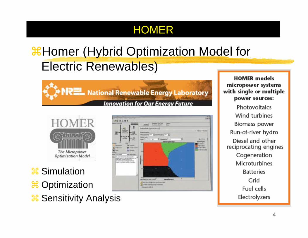
HOMER
Homer (Hybrid Optimization Model for Electric Renewables)
SimulationOptimizationSensitivity Analysis
4

Homer – a toolA tool for designing micropower systems
Village power systemsStand-alone applications and Hybrid SystemsMicro grid
5
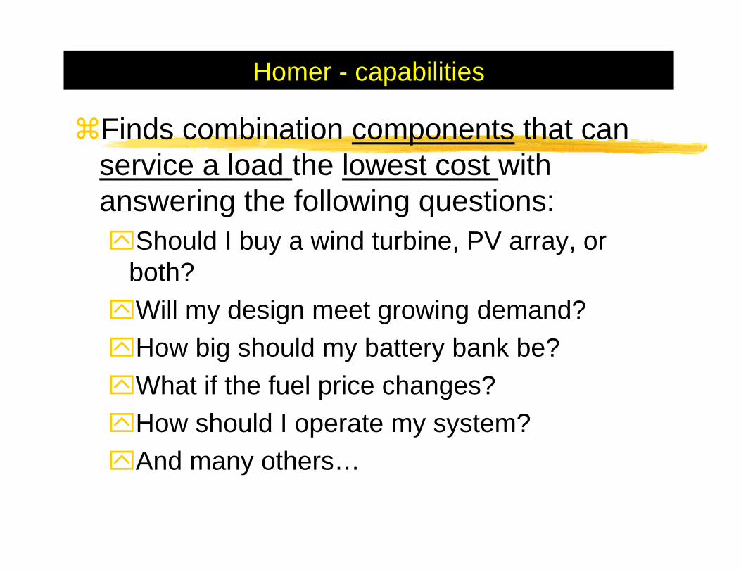
Homer - capabilities
Finds combination components that can service a load the lowest cost with answering the following questions:
Should I buy a wind turbine, PV array, or both?Will my design meet growing demand?How big should my battery bank be?What if the fuel price changes?How should I operate my system?And many others…
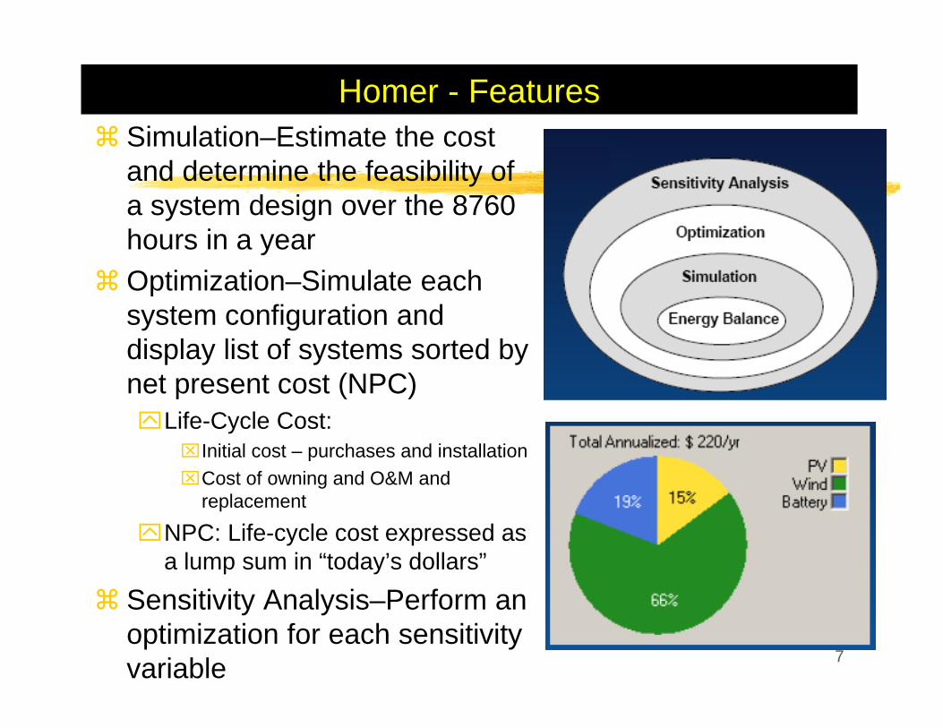
Homer - FeaturesSimulation–Estimate the cost and determine the feasibility of a system design over the 8760 hours in a yearOptimization–Simulate each system configuration and display list of systems sorted by net present cost (NPC)
Life-Cycle Cost:⌧Initial cost – purchases and installation⌧Cost of owning and O&M and
replacement
NPC: Life-cycle cost expressed as a lump sum in “today’s dollars”
Sensitivity Analysis–Perform an optimization for each sensitivity variable 7
8
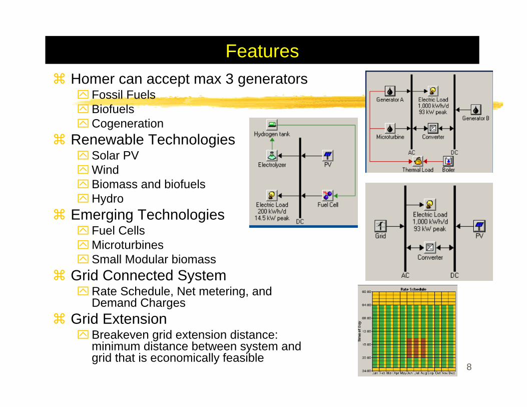
FeaturesHomer can accept max 3 generators
Fossil FuelsBiofuelsCogeneration
Renewable TechnologiesSolar PVWindBiomass and biofuelsHydro
Emerging TechnologiesFuel CellsMicroturbinesSmall Modular biomass
Grid Connected SystemRate Schedule, Net metering, and Demand Charges
Grid ExtensionBreakeven grid extension distance: minimum distance between system and grid that is economically feasible
Features
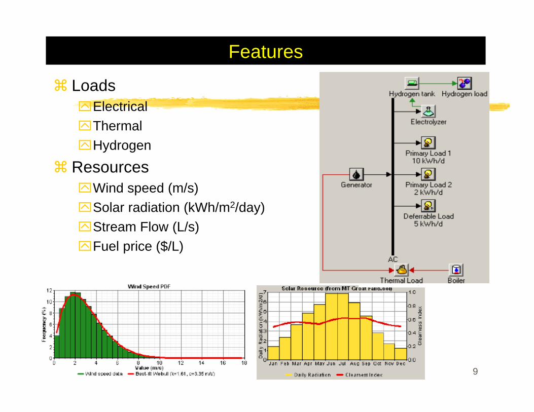
LoadsElectricalThermalHydrogen
ResourcesWind speed (m/s)Solar radiation (kWh/m2/day)Stream Flow (L/s)Fuel price ($/L)
9
How to use HOMER
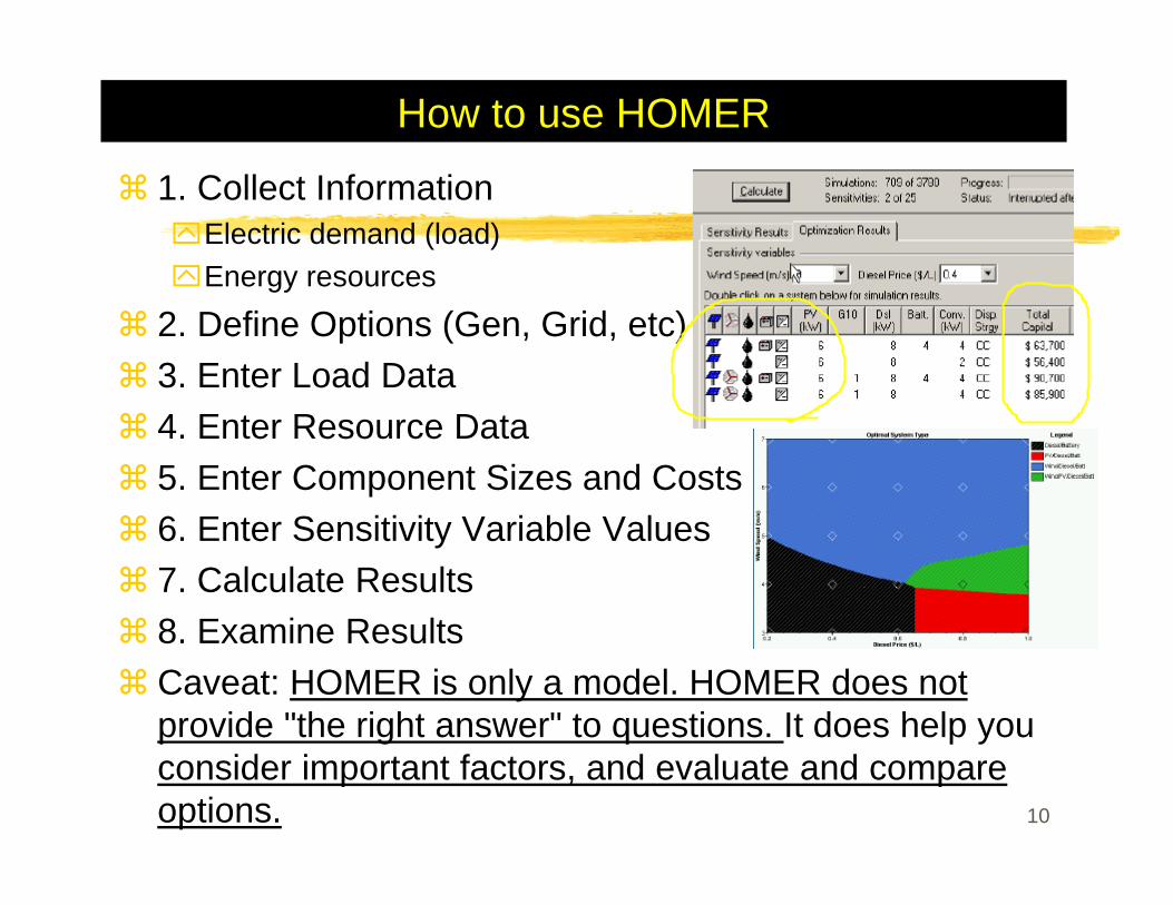
1. Collect InformationElectric demand (load)Energy resources
2. Define Options (Gen, Grid, etc)3. Enter Load Data4. Enter Resource Data5. Enter Component Sizes and Costs6. Enter Sensitivity Variable Values7. Calculate Results8. Examine ResultsCaveat: HOMER is only a model. HOMER does not provide "the right answer" to questions. It does help you consider important factors, and evaluate and compare options. 10
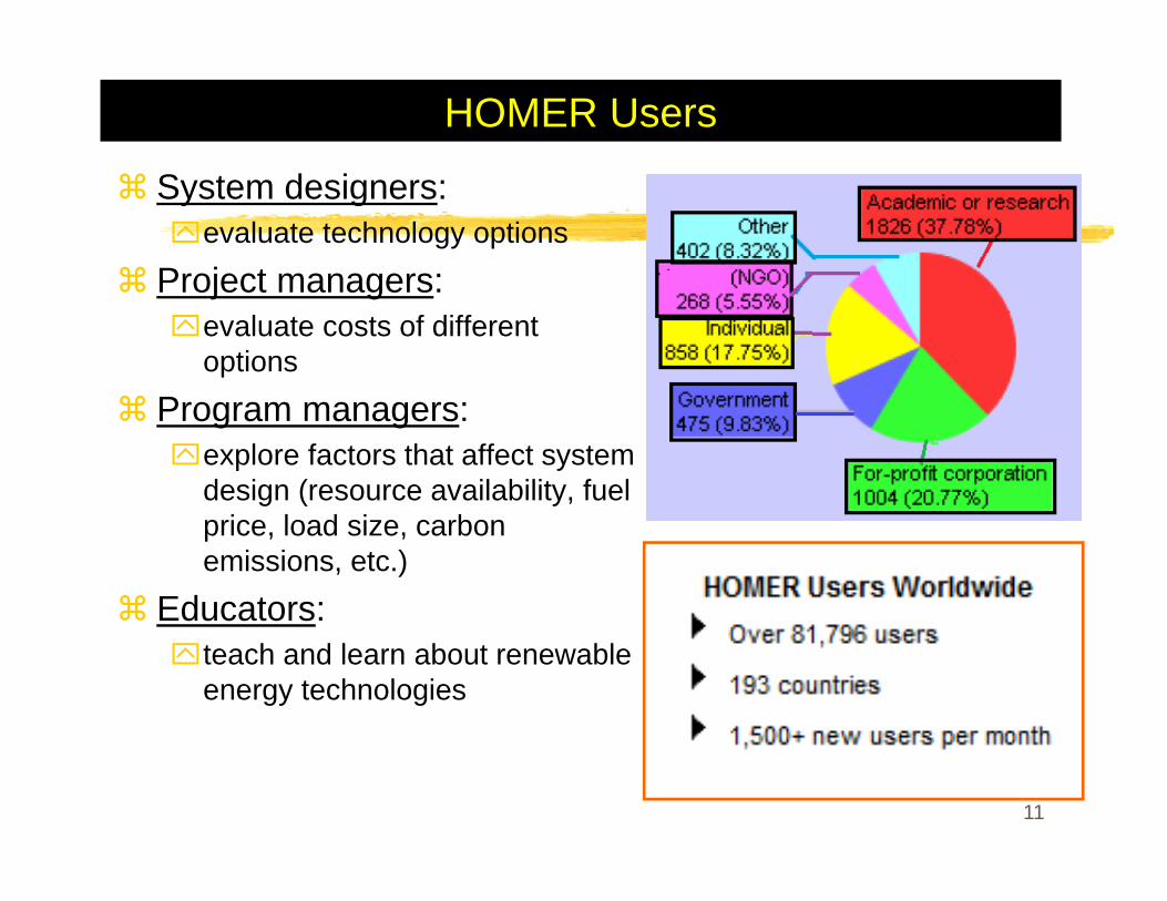
HOMER Users
System designers: evaluate technology options
Project managers: evaluate costs of different options
Program managers: explore factors that affect system design (resource availability, fuel price, load size, carbon emissions, etc.)
Educators: teach and learn about renewable energy technologies
11
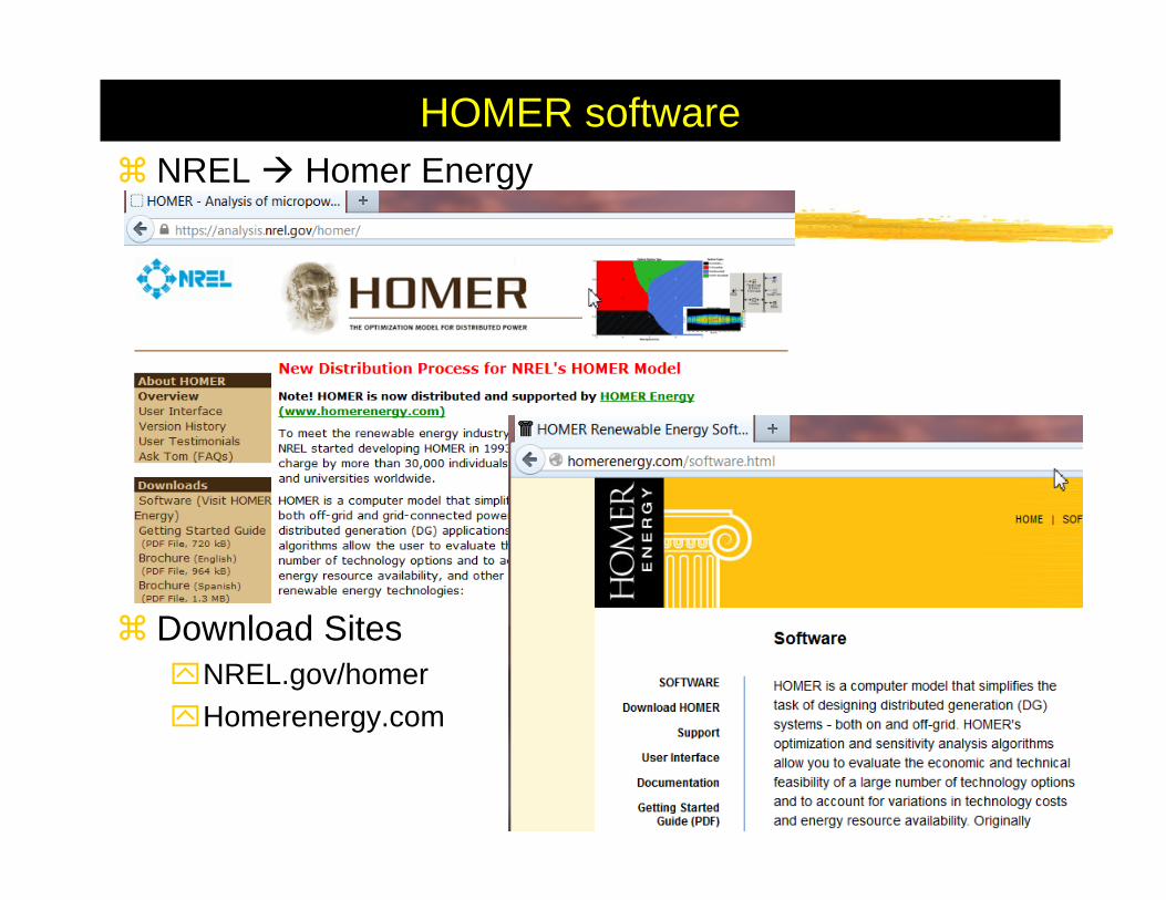
HOMER softwareNREL Homer Energy
Download SitesNREL.gov/homerHomerenergy.com
12
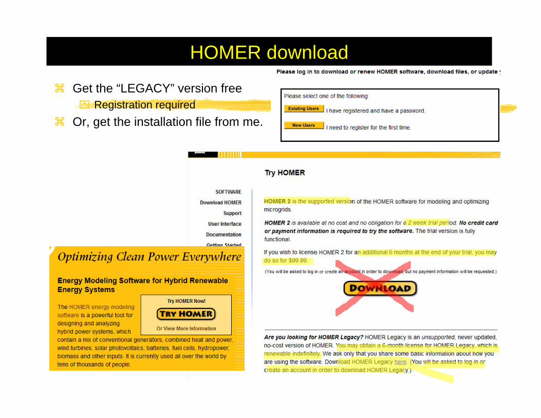
HOMER download
Get the “LEGACY” version freeRegistration required
Or, get the installation file from me.
13
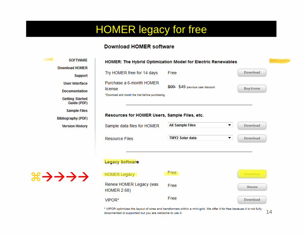
HOMER legacy for free
14
HOMER - Intro
HOMER (Hybrid Optimization Model for Electric Renewables): Micropower Optimization computer model developed by NREL.“Micropower system”: a system that generates electricity, and possibly heat, to serve a nearby load.Micro Grid
A solar–battery system serving a remote loada wind–diesel system serving an isolated villagea grid-connected natural gas micro-turbine providing electricity and heat to a factory.
Models power system’s physical behavior and its life-cycle cost [installation cost + O&M cost]Design options on technical and economic merit
15
HOMER – Principal 3 tasksSimulation: HOMER models the performance of a particular micropower system configuration each hour of the year to determine
its technical feasibility (i.e., it can adequately serve the electric and thermal loads and satisfy other constraints) and life-cycle cost.
Optimization: HOMER simulates many different system configurations in search of the one that satisfies the technical constraints at the lowest life-cycle cost.
Optimization determines the optimal value of the variables such as the mix of components that make up the system and the size or quantity of each.
Sensitivity Analysis: HOMER performs multiple optimizations under a range of input assumptions to gauge the effects of uncertainty or changes in the model inputs such as average wind speed or future fuel price
16
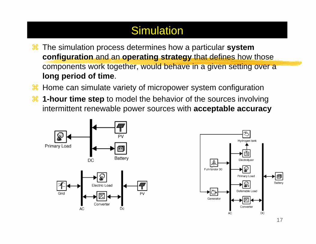
SimulationThe simulation process determines how a particular system configuration and an operating strategy that defines how those components work together, would behave in a given setting over a long period of time.Home can simulate variety of micropower system configuration1-hour time step to model the behavior of the sources involving intermittent renewable power sources with acceptable accuracy
17
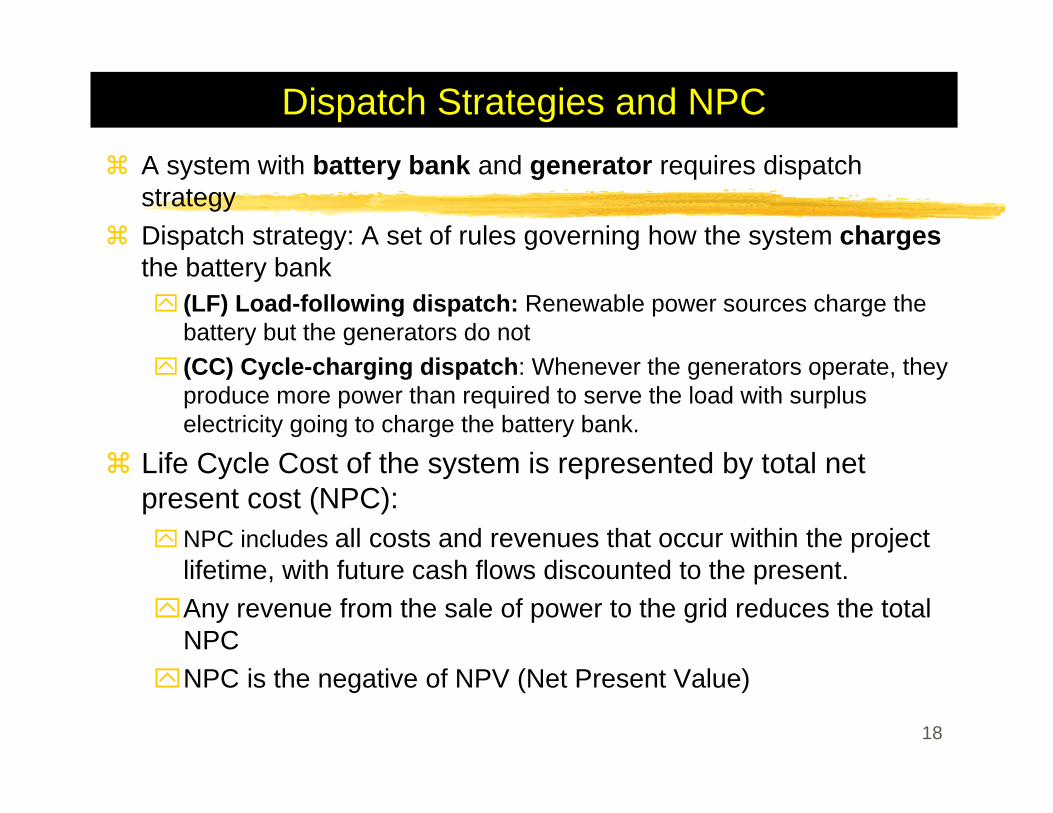
Dispatch Strategies and NPCA system with battery bank and generator requires dispatch strategyDispatch strategy: A set of rules governing how the system charges the battery bank
(LF) Load-following dispatch: Renewable power sources charge the battery but the generators do not(CC) Cycle-charging dispatch: Whenever the generators operate, they produce more power than required to serve the load with surplus electricity going to charge the battery bank.
Life Cycle Cost of the system is represented by total net present cost (NPC):
NPC includes all costs and revenues that occur within the project lifetime, with future cash flows discounted to the present.Any revenue from the sale of power to the grid reduces the total NPCNPC is the negative of NPV (Net Present Value)
18
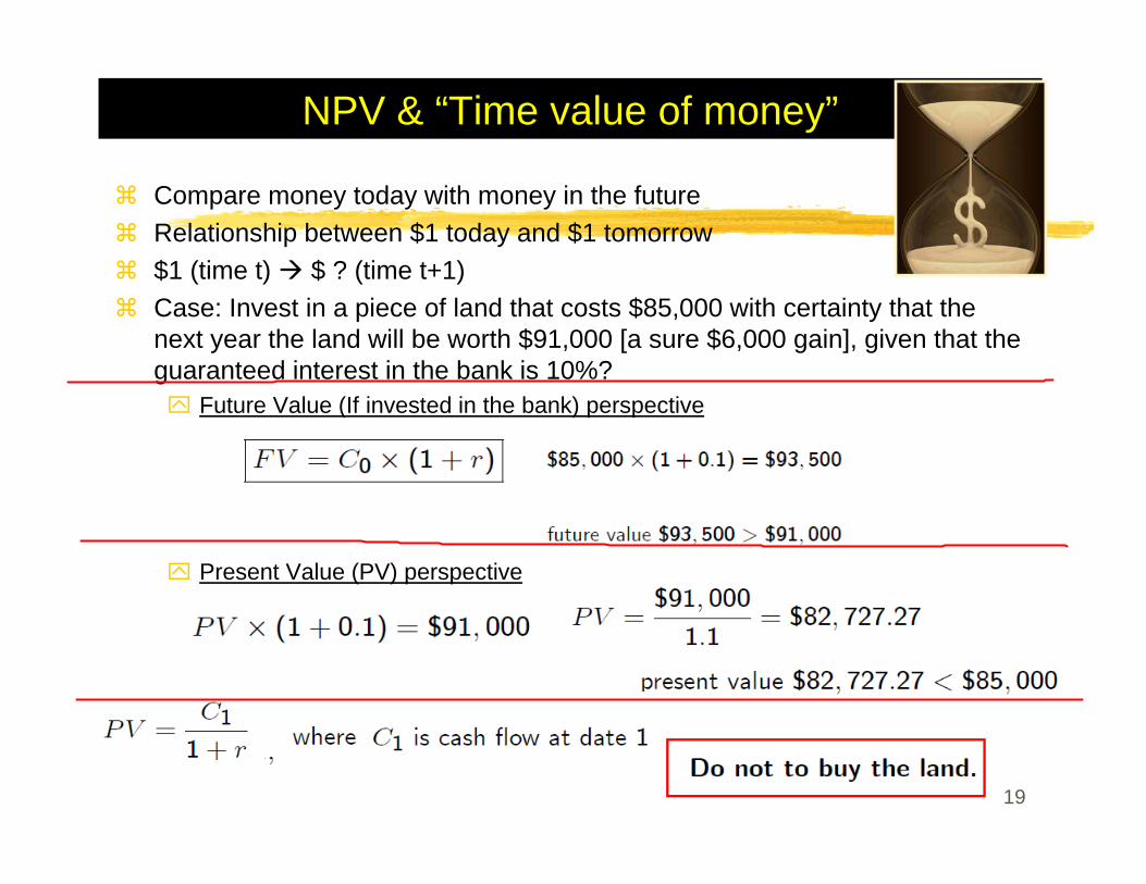
NPV & “Time value of money”
Compare money today with money in the futureRelationship between $1 today and $1 tomorrow$1 (time t) $ ? (time t+1)Case: Invest in a piece of land that costs $85,000 with certainty that the next year the land will be worth $91,000 [a sure $6,000 gain], given that the guaranteed interest in the bank is 10%?
Future Value (If invested in the bank) perspective
Present Value (PV) perspective
19
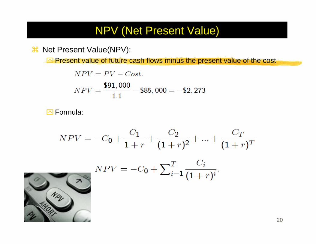
NPV (Net Present Value)Net Present Value(NPV):
Present value of future cash flows minus the present value of the cost
Formula:
20
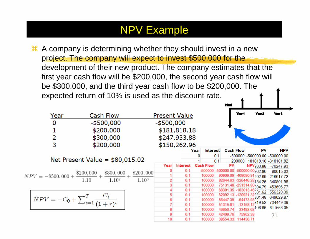
NPV ExampleA company is determining whether they should invest in a new project. The company will expect to invest $500,000 for the development of their new product. The company estimates that the first year cash flow will be $200,000, the second year cash flow will be $300,000, and the third year cash flow to be $200,000. The expected return of 10% is used as the discount rate.
21
Optimization
Best possible system configuration that satisfies the user-specified constraints at the lowest total net present cost.Decide on the mix of components that the system should contain, the size or quantity of each component, and the dispatch strategy (LF or CC) the system should use.Ranks the feasible ones according to total net present costPresents the feasible one with the lowest total net present cost as the optimal system configuration.
22
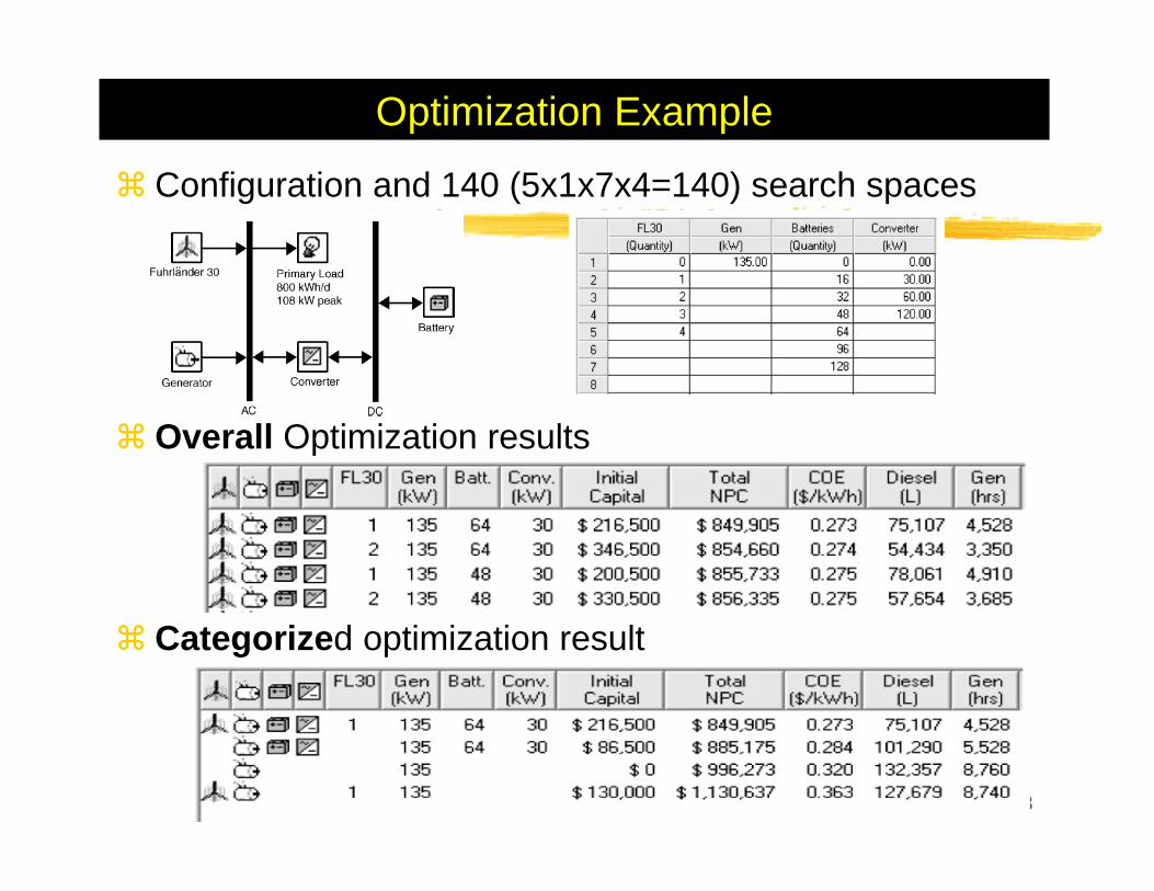
Optimization Example
Configuration and 140 (5x1x7x4=140) search spaces
Overall Optimization results
Categorized optimization result
23
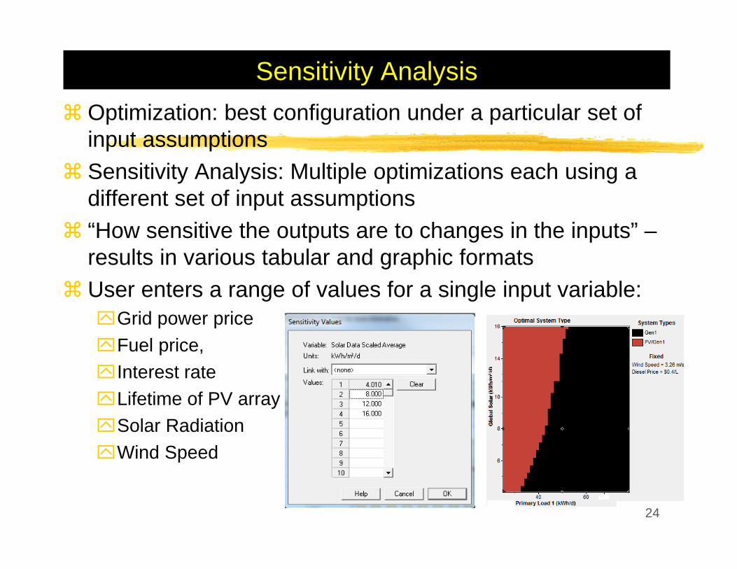
Sensitivity AnalysisOptimization: best configuration under a particular set of input assumptionsSensitivity Analysis: Multiple optimizations each using a different set of input assumptions“How sensitive the outputs are to changes in the inputs” –results in various tabular and graphic formatsUser enters a range of values for a single input variable:
Grid power priceFuel price,Interest rateLifetime of PV arraySolar RadiationWind Speed
24
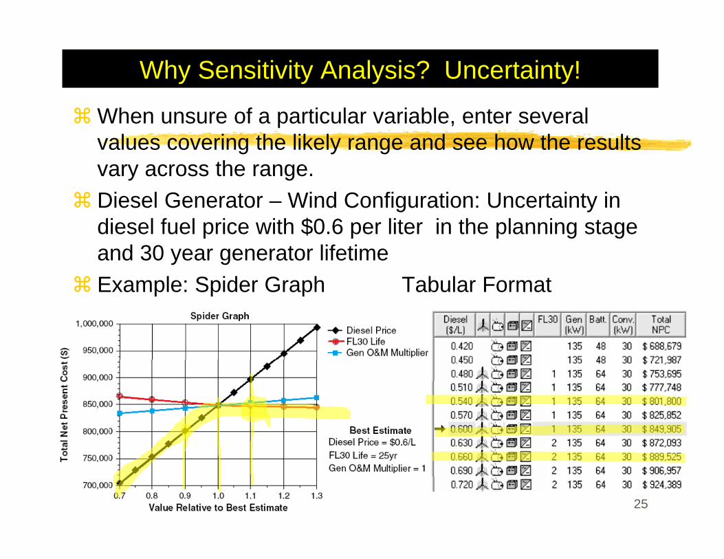
Why Sensitivity Analysis? Uncertainty!
When unsure of a particular variable, enter several values covering the likely range and see how the results vary across the range.Diesel Generator – Wind Configuration: Uncertainty in diesel fuel price with $0.6 per liter in the planning stage and 30 year generator lifetimeExample: Spider Graph Tabular Format
25
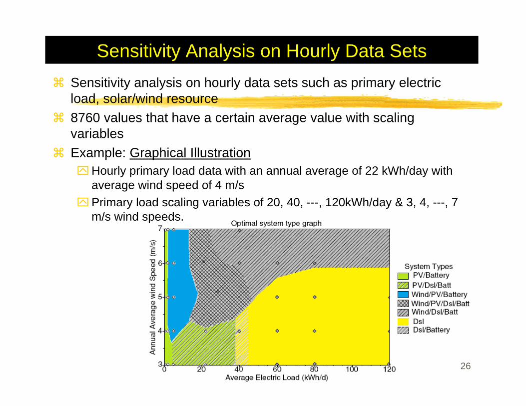
Sensitivity Analysis on Hourly Data SetsSensitivity analysis on hourly data sets such as primary electric load, solar/wind resource8760 values that have a certain average value with scaling variablesExample: Graphical Illustration
Hourly primary load data with an annual average of 22 kWh/day with average wind speed of 4 m/sPrimary load scaling variables of 20, 40, ---, 120kWh/day & 3, 4, ---, 7 m/s wind speeds.
26
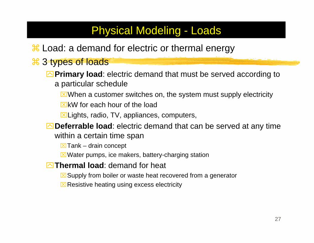
Physical Modeling - LoadsLoad: a demand for electric or thermal energy3 types of loads
Primary load: electric demand that must be served according to a particular schedule⌧When a customer switches on, the system must supply electricity⌧kW for each hour of the load⌧Lights, radio, TV, appliances, computers,
Deferrable load: electric demand that can be served at any time within a certain time span⌧Tank – drain concept⌧Water pumps, ice makers, battery-charging station
Thermal load: demand for heat⌧Supply from boiler or waste heat recovered from a generator⌧Resistive heating using excess electricity
27
Physical Modeling - Resources
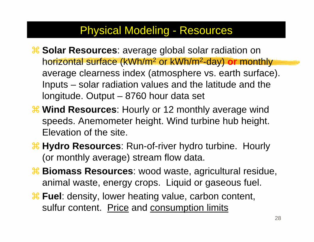
Solar Resources: average global solar radiation on horizontal surface (kWh/m2 or kWh/m2-day) or monthly average clearness index (atmosphere vs. earth surface). Inputs – solar radiation values and the latitude and the longitude. Output – 8760 hour data set Wind Resources: Hourly or 12 monthly average wind speeds. Anemometer height. Wind turbine hub height. Elevation of the site.Hydro Resources: Run-of-river hydro turbine. Hourly (or monthly average) stream flow data. Biomass Resources: wood waste, agricultural residue, animal waste, energy crops. Liquid or gaseous fuel. Fuel: density, lower heating value, carbon content, sulfur content. Price and consumption limits
28
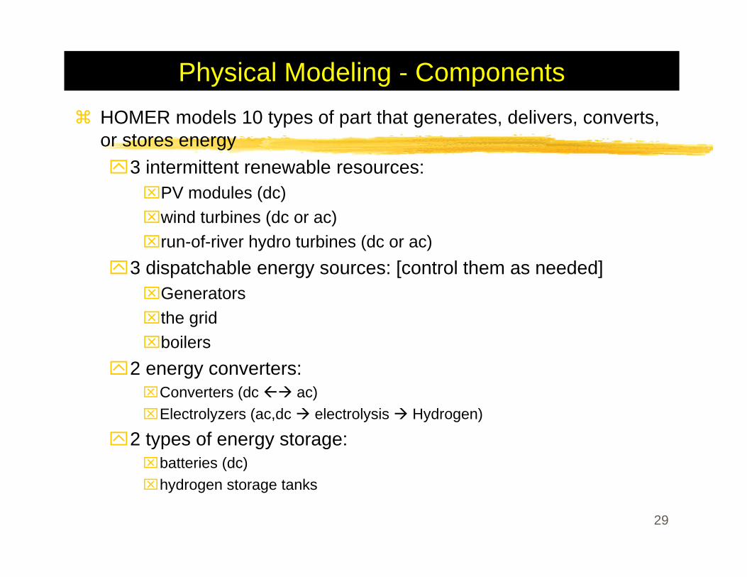
Physical Modeling - ComponentsHOMER models 10 types of part that generates, delivers, converts, or stores energy
3 intermittent renewable resources: ⌧PV modules (dc)⌧wind turbines (dc or ac)⌧run-of-river hydro turbines (dc or ac)
3 dispatchable energy sources: [control them as needed] ⌧Generators⌧the grid⌧boilers
2 energy converters: ⌧Converters (dc ac) ⌧Electrolyzers (ac,dc electrolysis Hydrogen)
2 types of energy storage: ⌧batteries (dc) ⌧hydrogen storage tanks
29
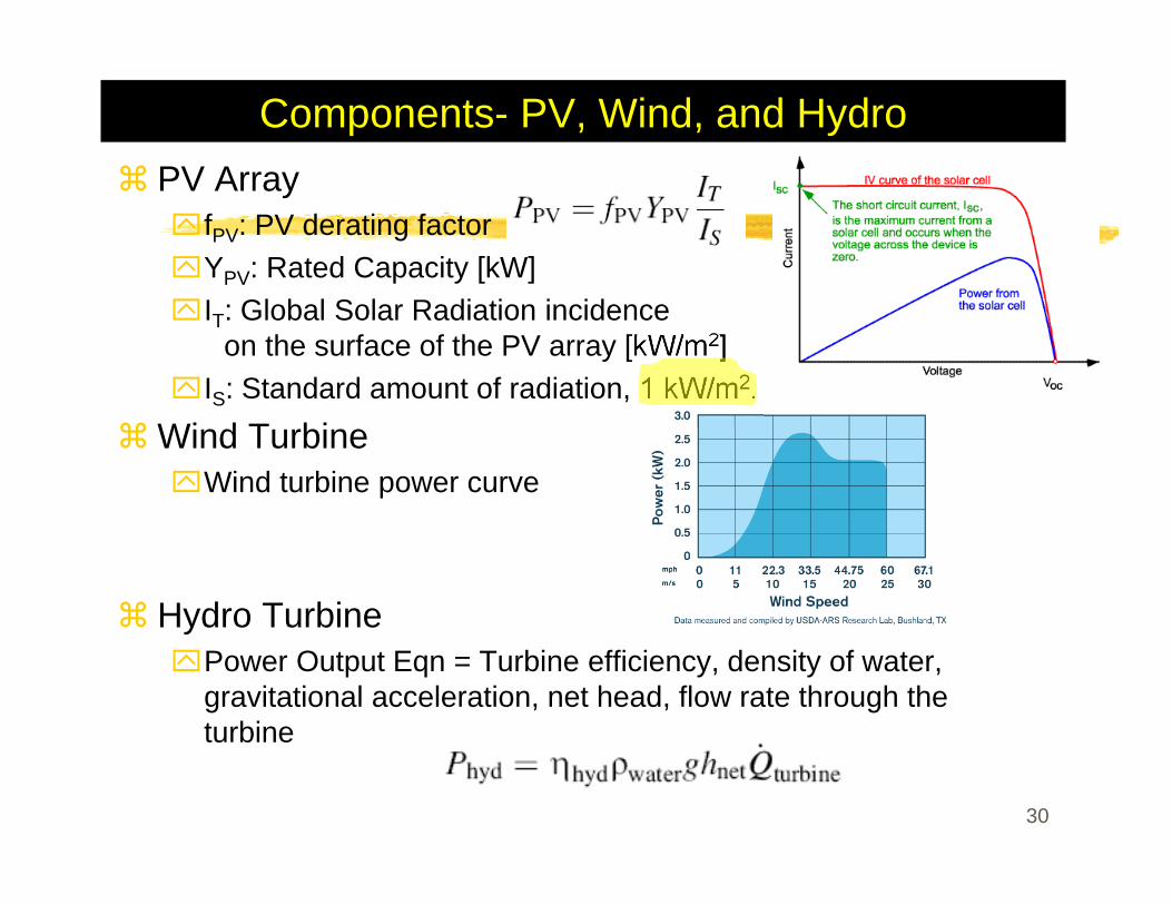
Components- PV, Wind, and HydroPV Array
fPV: PV derating factorYPV: Rated Capacity [kW]IT: Global Solar Radiation incidence
on the surface of the PV array [kW/m2]IS: Standard amount of radiation, 1 kW/m2.
Wind TurbineWind turbine power curve
Hydro TurbinePower Output Eqn = Turbine efficiency, density of water, gravitational acceleration, net head, flow rate through the turbine
30
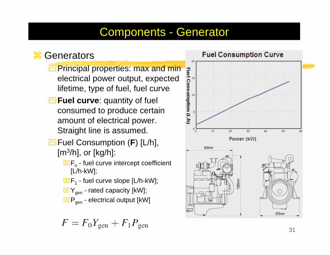
Components - Generator
GeneratorsPrincipal properties: max and min electrical power output, expected lifetime, type of fuel, fuel curveFuel curve: quantity of fuel consumed to produce certain amount of electrical power. Straight line is assumed.Fuel Consumption (F) [L/h], [m3/h], or [kg/h]:⌧Fo - fuel curve intercept coefficient
[L/h-kW]; ⌧F1 - fuel curve slope [L/h-kW]; ⌧Ygen - rated capacity [kW]; ⌧Pgen - electrical output [kW]
31
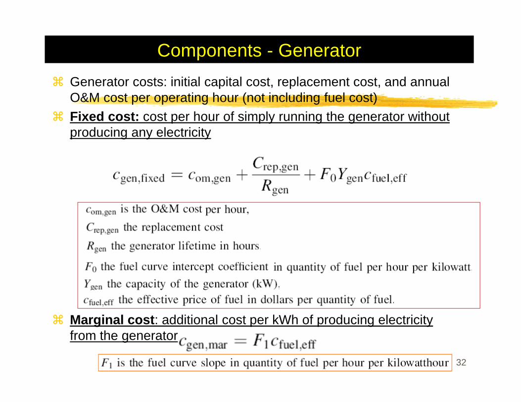
Components - GeneratorGenerator costs: initial capital cost, replacement cost, and annual O&M cost per operating hour (not including fuel cost)Fixed cost: cost per hour of simply running the generator without producing any electricity
Marginal cost: additional cost per kWh of producing electricity from the generator
32
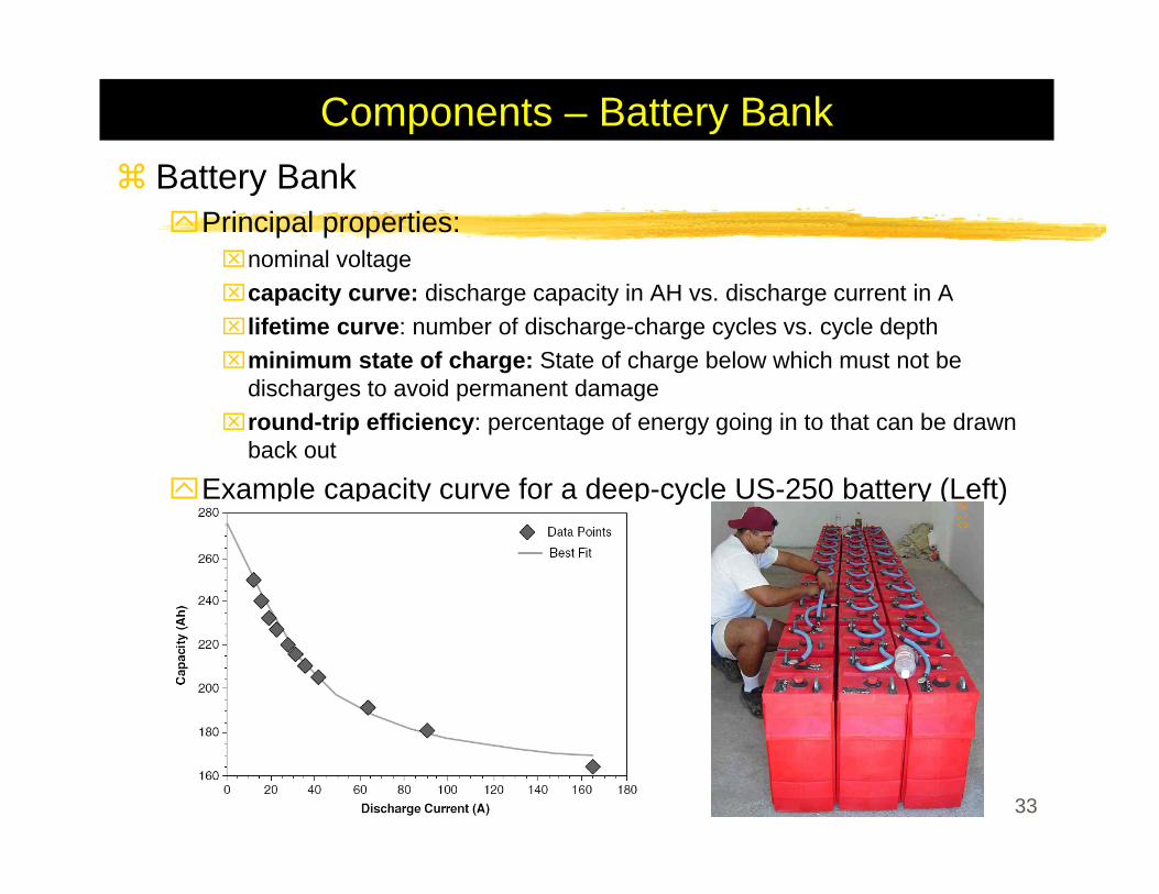
Components – Battery BankBattery Bank
Principal properties: ⌧nominal voltage⌧capacity curve: discharge capacity in AH vs. discharge current in A⌧lifetime curve: number of discharge-charge cycles vs. cycle depth ⌧minimum state of charge: State of charge below which must not be
discharges to avoid permanent damage⌧round-trip efficiency: percentage of energy going in to that can be drawn
back out
Example capacity curve for a deep-cycle US-250 battery (Left)
33
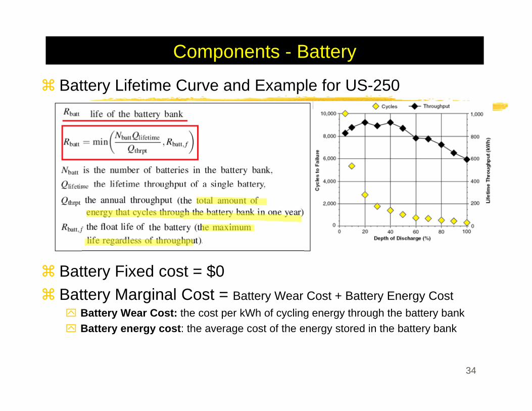
Components - Battery
Battery Lifetime Curve and Example for US-250
Battery Fixed cost = $0Battery Marginal Cost = Battery Wear Cost + Battery Energy Cost
Battery Wear Cost: the cost per kWh of cycling energy through the battery bankBattery energy cost: the average cost of the energy stored in the battery bank
34
Components - BatteryBattery energy cost each hour: dividing the total year-to-date cost of charging the battery bank by the total year-to-date amount of energy put into the battery bank
Load-following dispatch strategy: since charged only by surplus electricity, charging cost of battery is always zeroCycle-charging strategy: charging cost is not zero.
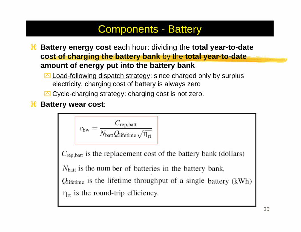
Battery wear cost:
35
Components - GridGrid and Grid Power Cost
Grid power price [$/kWh]: charges for energy purchase from gridDemand rate [$/kW/month]: peak grid demandSellback rate [$/kWh]: price the utility pays for the power sold to grid
Net Metering: a billing arrangement whereby the utility charges the customer based on the net grid purchases (purchases minus sales) over the billing period.
Purchase > sales: consumer pays the utility an amount equal to the net grid purchases times the grid power cost. sales > purchases: the utility pays the consumer an amount equal to the net grid sales (sales minus purchases) times the sellback rate, which is typically less than the grid power price, and often zero.
Grid fixed cost: $0Grid marginal cost: current grid power price plus any cost resulting from emissions penalties.
36
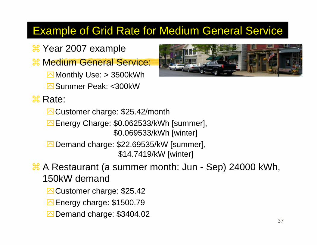
Example of Grid Rate for Medium General ServiceYear 2007 exampleMedium General Service:
Monthly Use: > 3500kWhSummer Peak: <300kW
Rate: Customer charge: $25.42/monthEnergy Charge: $0.062533/kWh [summer],
$0.069533/kWh [winter]Demand charge: $22.69535/kW [summer],
$14.7419/kW [winter]
A Restaurant (a summer month: Jun - Sep) 24000 kWh, 150kW demand
Customer charge: $25.42Energy charge: $1500.79Demand charge: $3404.02
37
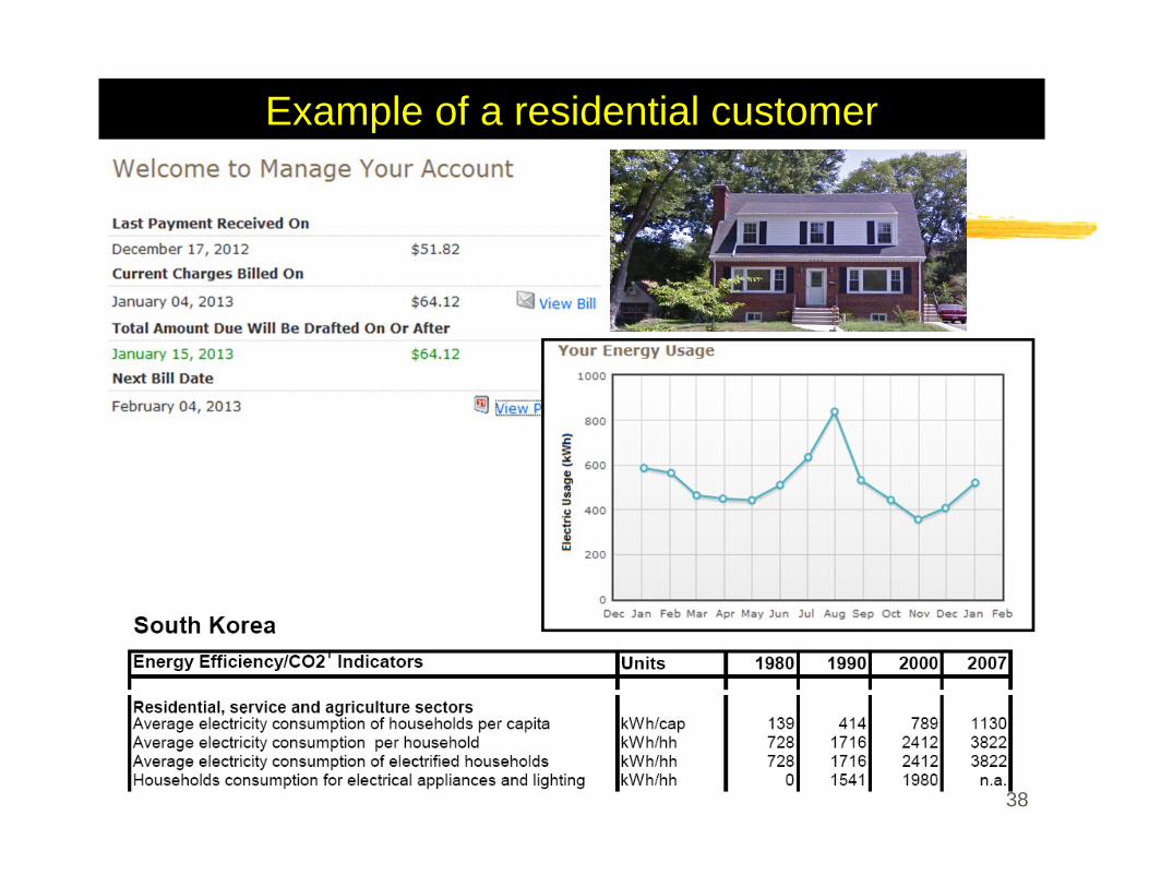
Example of a residential customer
38
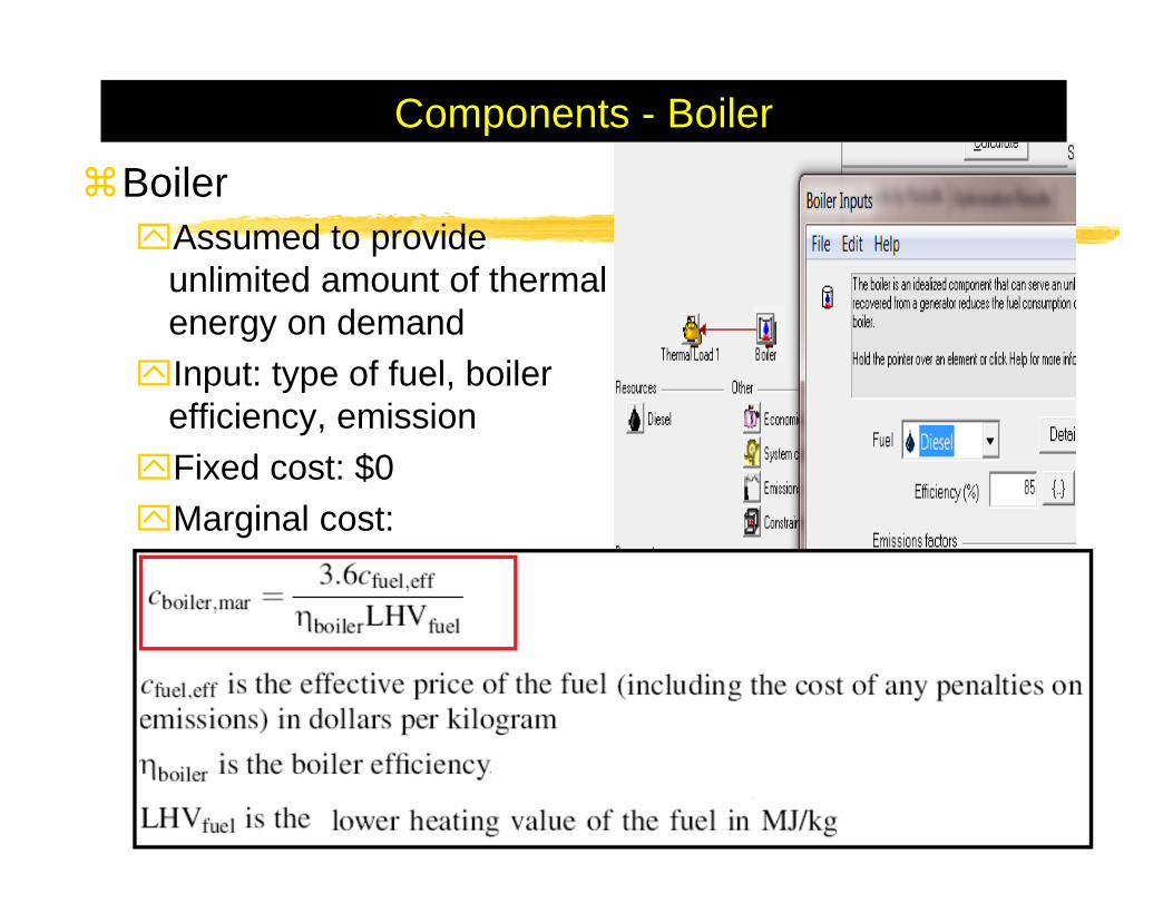
Components - Boiler
BoilerAssumed to provide unlimited amount of thermal energy on demandInput: type of fuel, boiler efficiency, emissionFixed cost: $0Marginal cost:
39
Heating Value of Fuel
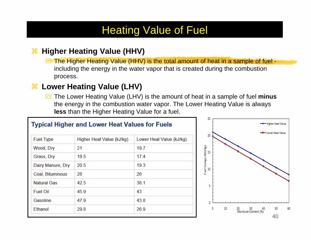
Higher Heating Value (HHV) The Higher Heating Value (HHV) is the total amount of heat in a sample of fuel -including the energy in the water vapor that is created during the combustion process.
Lower Heating Value (LHV) The Lower Heating Value (LHV) is the amount of heat in a sample of fuel minusthe energy in the combustion water vapor. The Lower Heating Value is always less than the Higher Heating Value for a fuel.
40
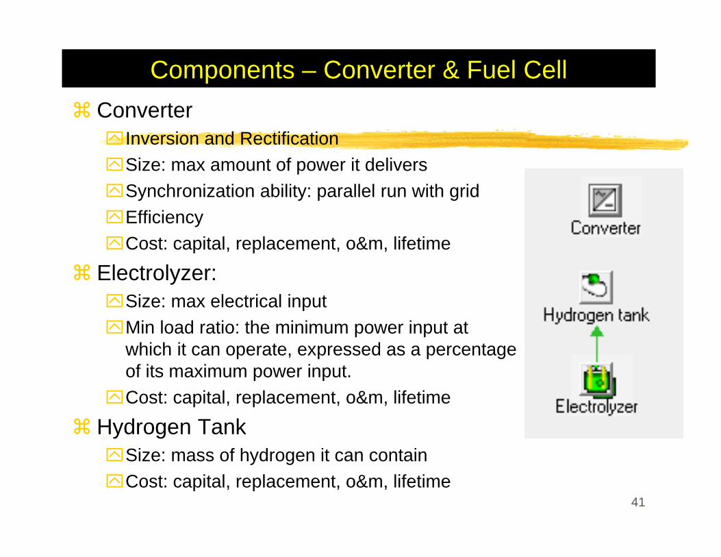
Components – Converter & Fuel CellConverter
Inversion and RectificationSize: max amount of power it deliversSynchronization ability: parallel run with gridEfficiencyCost: capital, replacement, o&m, lifetime
Electrolyzer:Size: max electrical inputMin load ratio: the minimum power input at which it can operate, expressed as a percentage of its maximum power input.Cost: capital, replacement, o&m, lifetime
Hydrogen TankSize: mass of hydrogen it can containCost: capital, replacement, o&m, lifetime
41
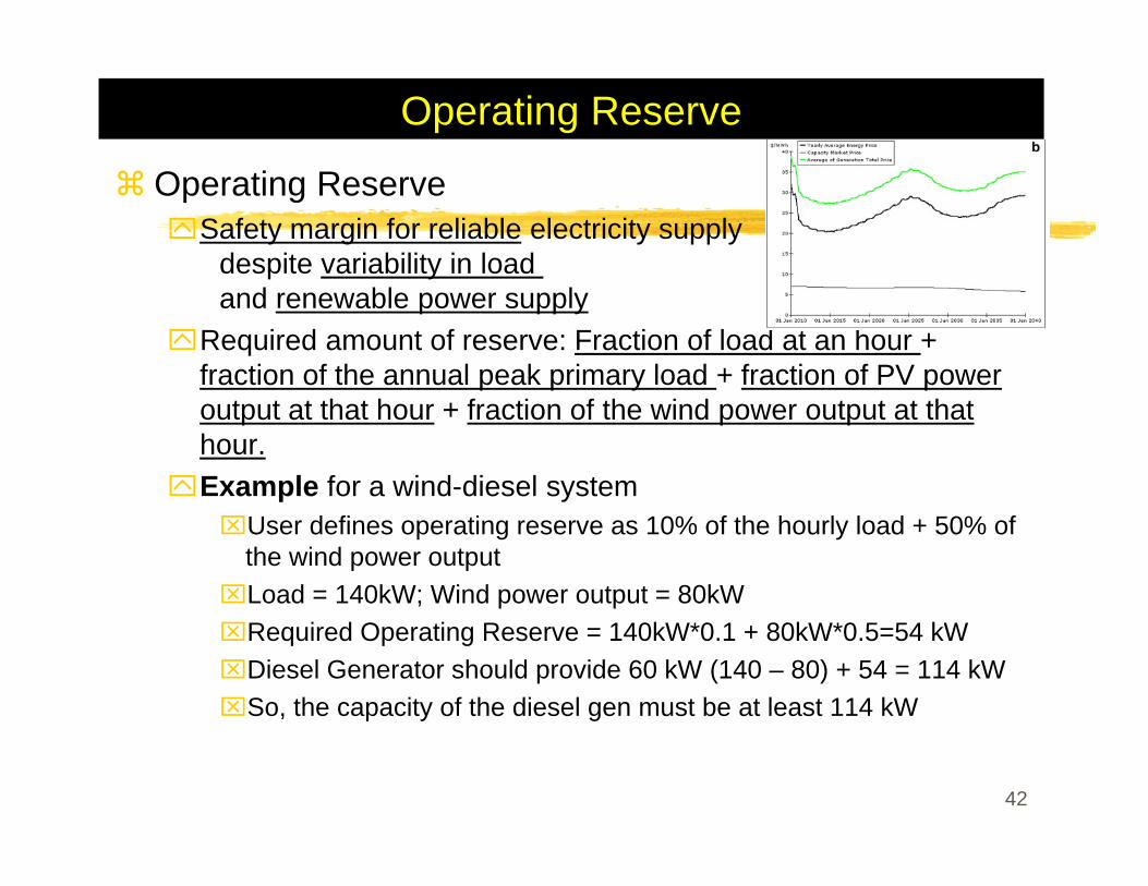
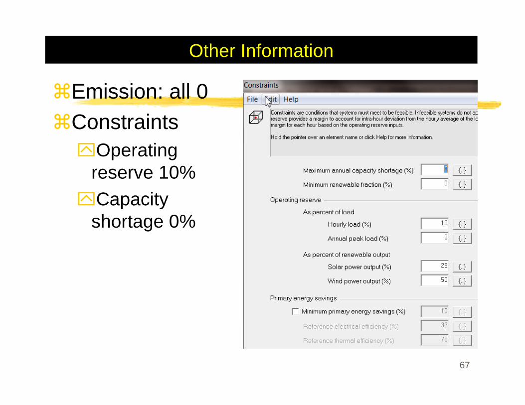
Operating Reserve
Operating ReserveSafety margin for reliable electricity supply
despite variability in load and renewable power supply
Required amount of reserve: Fraction of load at an hour + fraction of the annual peak primary load + fraction of PV power output at that hour + fraction of the wind power output at that hour.Example for a wind-diesel system⌧User defines operating reserve as 10% of the hourly load + 50% of
the wind power output⌧Load = 140kW; Wind power output = 80kW⌧Required Operating Reserve = 140kW*0.1 + 80kW*0.5=54 kW⌧Diesel Generator should provide 60 kW (140 – 80) + 54 = 114 kW ⌧So, the capacity of the diesel gen must be at least 114 kW
42
System DispatchDispatachable and non-dispatchable power sourcesDispatchable source: provides operating capacity in an amount equal to the maximum amount of power it could produce at a moment’s notice.
Generator⌧ In operation: dispatchable opr capacity = rated capacity⌧ non-operation: dispatchable opr capacity = 0
Grid: dispatchable opr capacity = max grid demandBattery: dispatachable opr capacity = current max discharge power
Non-dispatchable sourceOperating capacity (PV, Wind, or Hydro) = the amount the source is currently producing (Not the max amount it can produce)
NOTE: If a system is ever unable to supply the required amount of load plus operating reserve, HOMER records the shortfall as “capacity shortage”.
HOMER calculates the total amount of such shortages over the year and divides the total annual capacity shortage by the total annual electric load.
43
Dispatch Strategy for a system with Gen and Battery
Dispatch StrategyWhether and how the generator should charge the battery bank?There is no deterministic way to calculate the value of charging the battery bank – the value of charging in one hour depends on what happens in future hours. [enter Wind power which can provide enough power the next hour – then the diesel power into battery would be wasted]HOMER provides 2 simple strategies and lets user model them both to see which is better in any particular situation.⌧Load-following: a generator produces only enough power to serve the
load, and does not charge the battery bank.⌧Cycle-Charging: whenever a generator operates, it runs at its maximum rated
capacity and charges the battery bank with the excess⌧It was found that over a wide range of conditions, the better of these
two simple strategies is virtually as cost-effective as the ideal predictive strategy.
“Set-point state charge”: in the cycle-charging strategy, generator charges until the battery reaches the set-point state of charge. 44
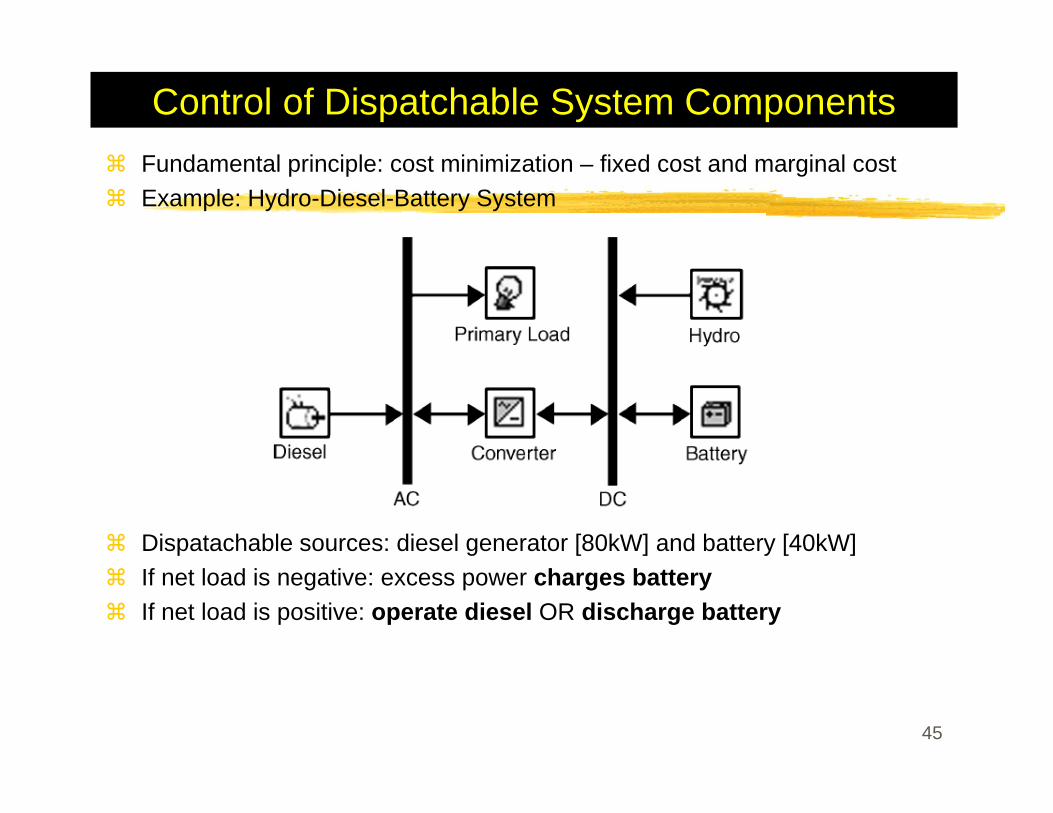
Control of Dispatchable System ComponentsFundamental principle: cost minimization – fixed cost and marginal costExample: Hydro-Diesel-Battery System
Dispatachable sources: diesel generator [80kW] and battery [40kW]If net load is negative: excess power charges batteryIf net load is positive: operate diesel OR discharge battery
45
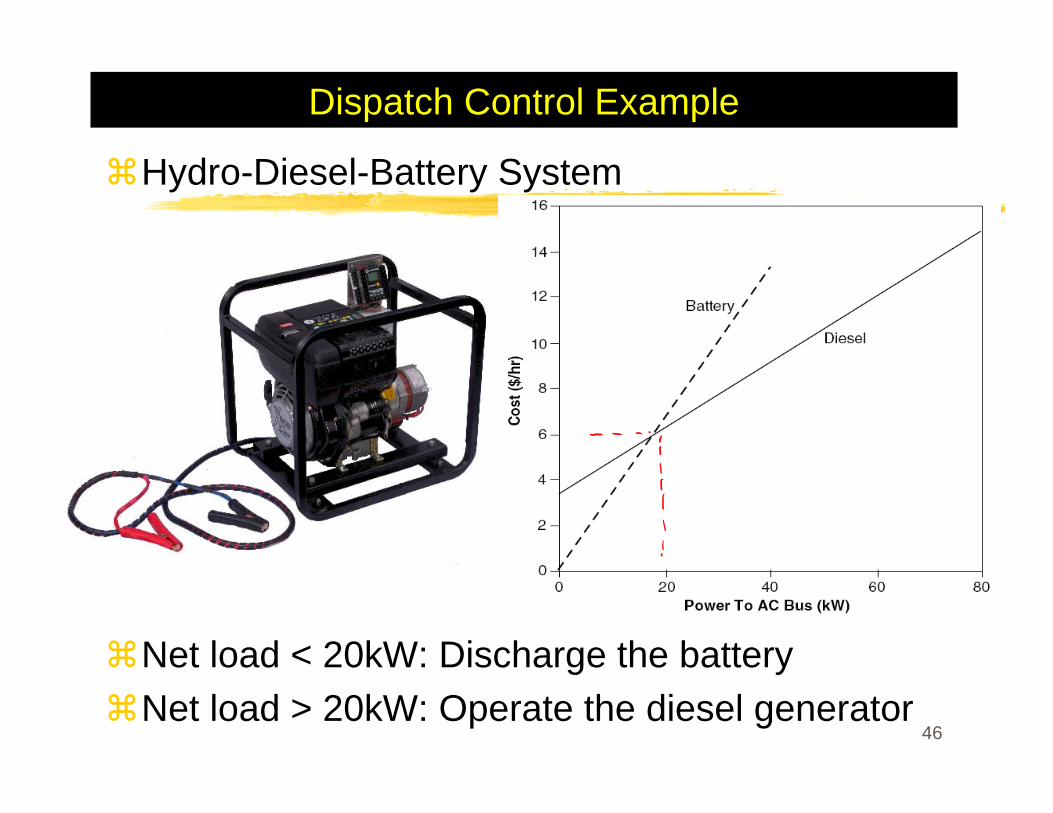
Dispatch Control Example
Hydro-Diesel-Battery System
Net load < 20kW: Discharge the batteryNet load > 20kW: Operate the diesel generator
46
Load Priority
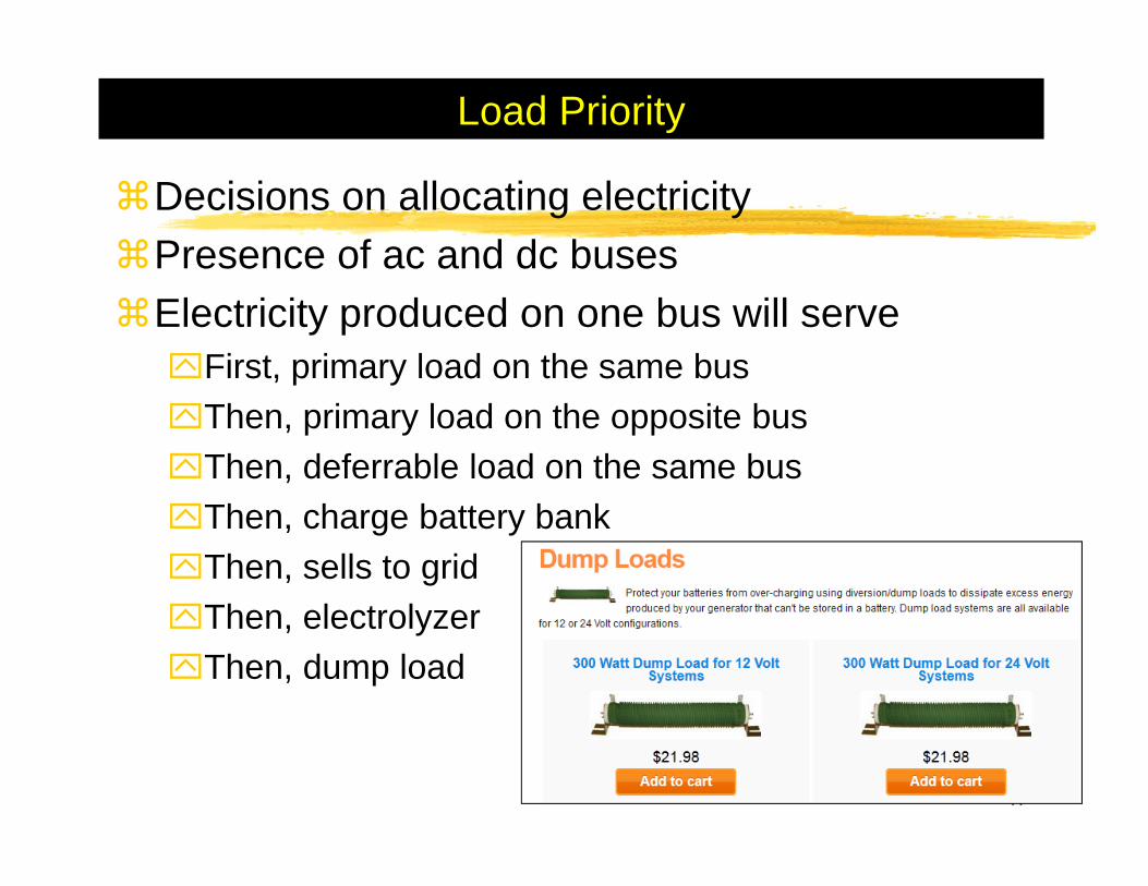
Decisions on allocating electricity Presence of ac and dc busesElectricity produced on one bus will serve
First, primary load on the same busThen, primary load on the opposite busThen, deferrable load on the same busThen, charge battery bankThen, sells to gridThen, electrolyzerThen, dump load
47
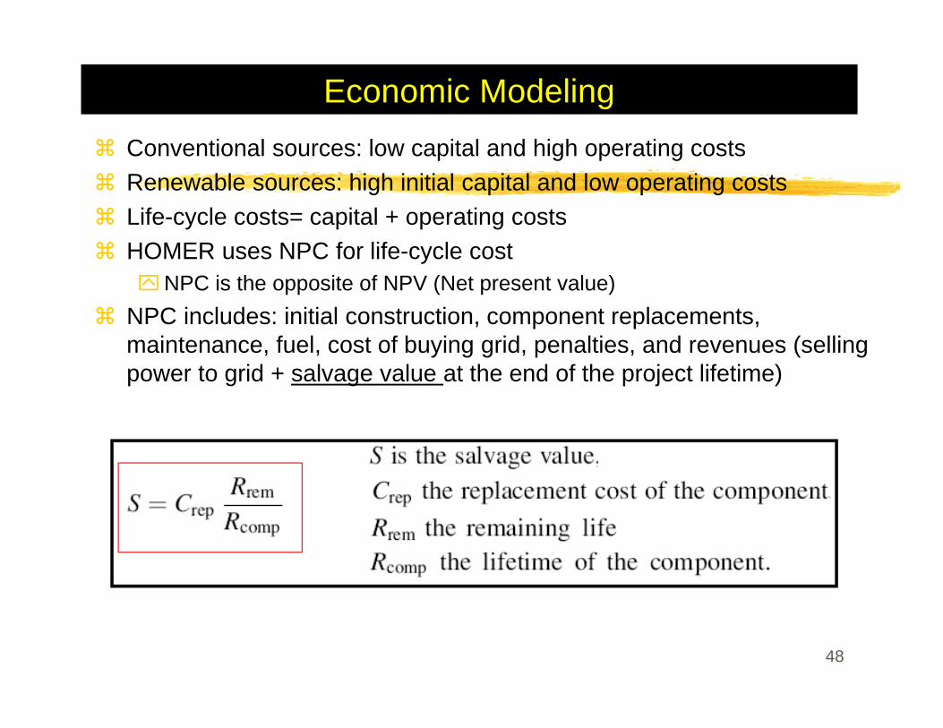
Economic ModelingConventional sources: low capital and high operating costsRenewable sources: high initial capital and low operating costsLife-cycle costs= capital + operating costsHOMER uses NPC for life-cycle cost
NPC is the opposite of NPV (Net present value)NPC includes: initial construction, component replacements, maintenance, fuel, cost of buying grid, penalties, and revenues (selling power to grid + salvage value at the end of the project lifetime)
48
Real Cost
All price escalates at the same rate over the lifetimeInflation can be factored out of analysis by using the real (inflation-adjusted) interest rate (rather than nominal interest rate) when discounting the future cash flows to the presentReal interest rate = nominal interest rate –inflation rateReal cost in terms of constant dollars
49
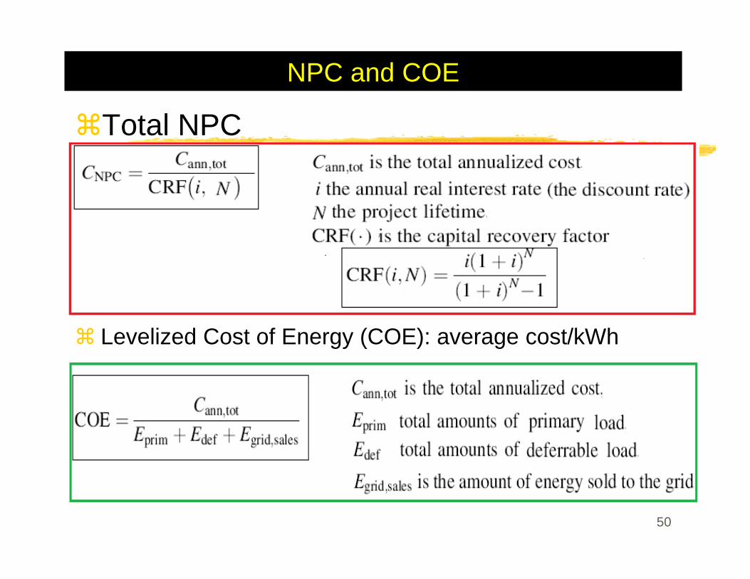
NPC and COE
Total NPC
Levelized Cost of Energy (COE): average cost/kWh
50
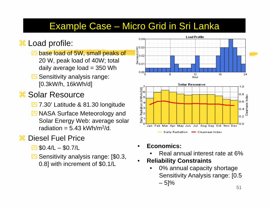
Example Case – Micro Grid in Sri Lanka
Load profile: base load of 5W, small peaks of 20 W, peak load of 40W; total daily average load = 350 WhSensitivity analysis range: [0.3kW/h, 16kWh/d]
Solar Resource7.30’ Latitude & 81.30 longitudeNASA Surface Meteorology and Solar Energy Web: average solar radiation = 5.43 kWh/m2/d.
Diesel Fuel Price$0.4/L – $0.7/LSensitivity analysis range: [$0.3, 0.8] with increment of $0.1/L
51
• Economics:• Real annual interest rate at 6%
• Reliability Constraints• 0% annual capacity shortage
Sensitivity Analysis range: [0.5 – 5]%
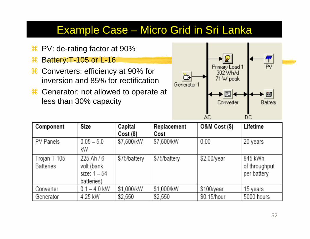
Example Case – Micro Grid in Sri LankaPV: de-rating factor at 90%Battery:T-105 or L-16Converters: efficiency at 90% for inversion and 85% for rectificationGenerator: not allowed to operate at less than 30% capacity
52
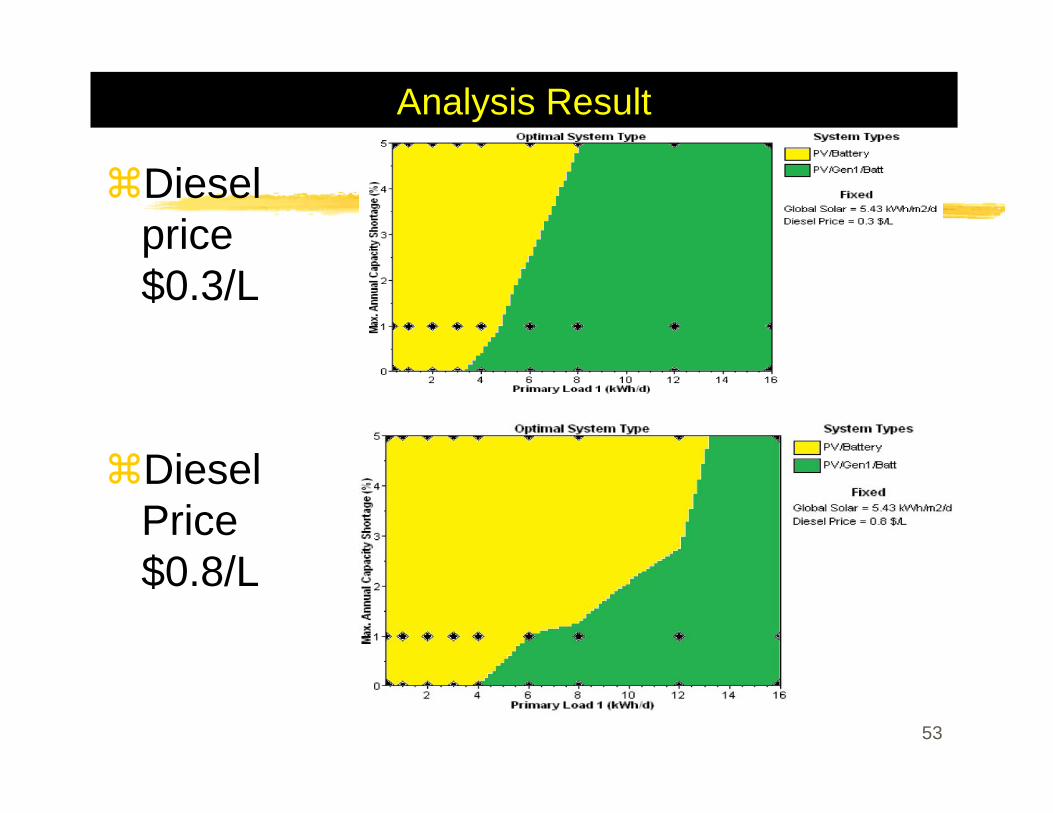
Analysis Result
Diesel price $0.3/L
Diesel Price $0.8/L
53
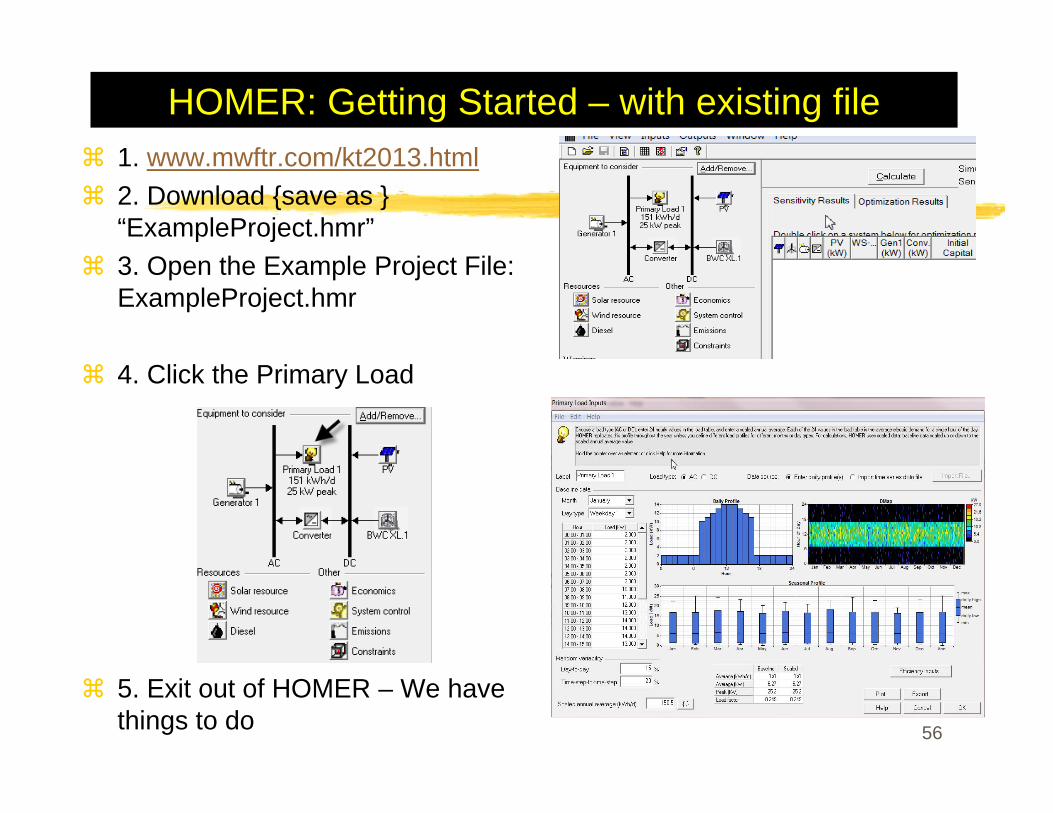
HOMER: Getting Started – with existing file1. www.mwftr.com/kt2013.html2. Download {save as } “ExampleProject.hmr”3. Open the Example Project File: ExampleProject.hmr
4. Click the Primary Load
5. Exit out of HOMER – We have things to do 56
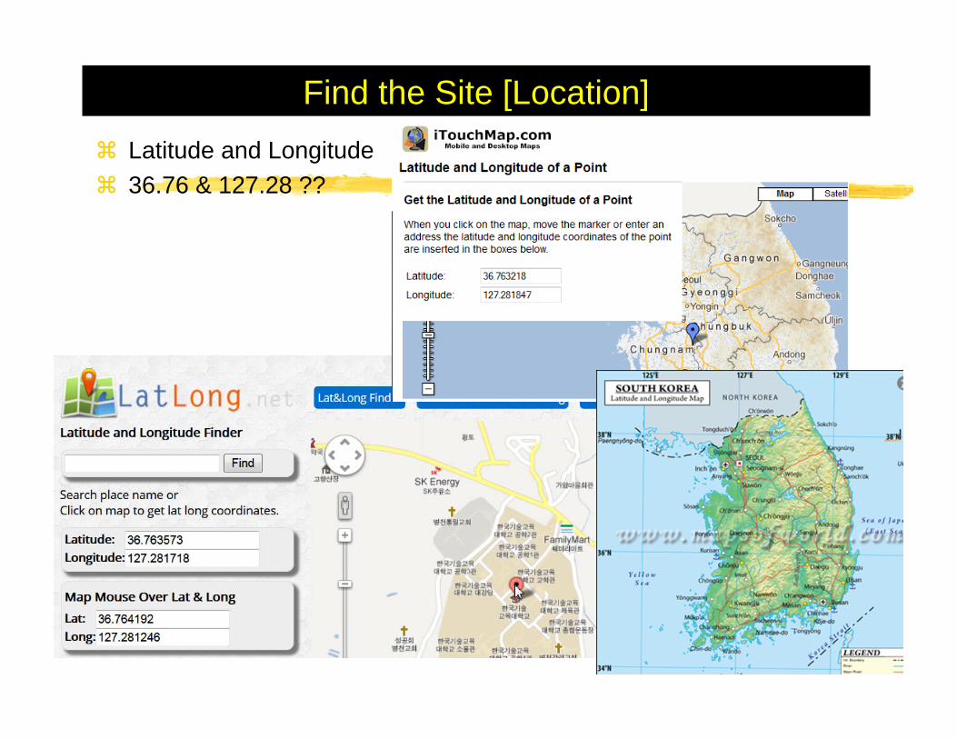
Find the Site [Location]Latitude and Longitude36.76 & 127.28 ??
57
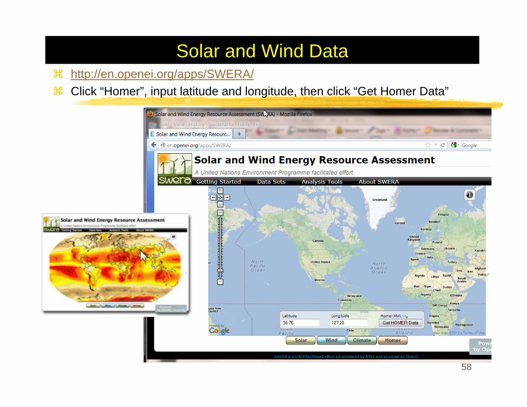
Solar and Wind Datahttp://en.openei.org/apps/SWERA/Click “Homer”, input latitude and longitude, then click “Get Homer Data”
58
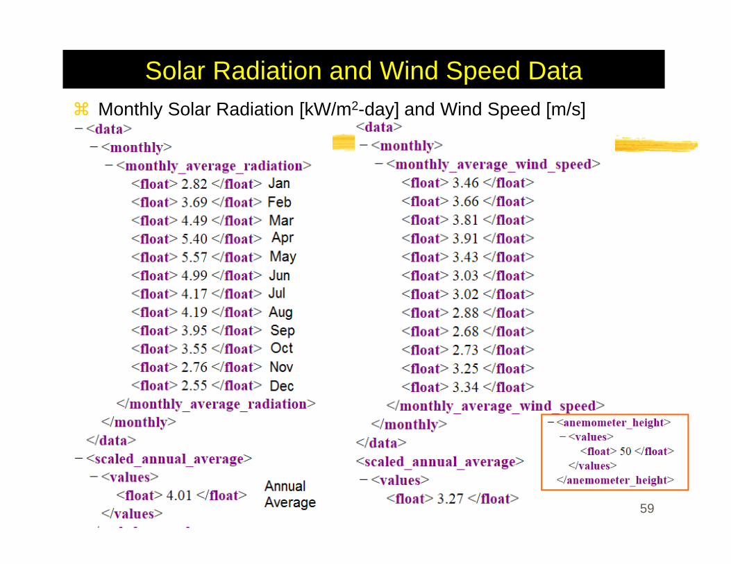
Solar Radiation and Wind Speed DataMonthly Solar Radiation [kW/m2-day] and Wind Speed [m/s]
59
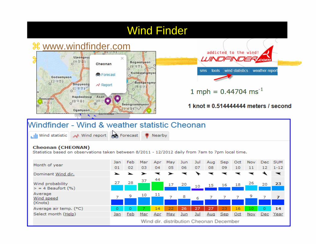
Wind Finderwww.windfinder.comClick Wind Statistics
60
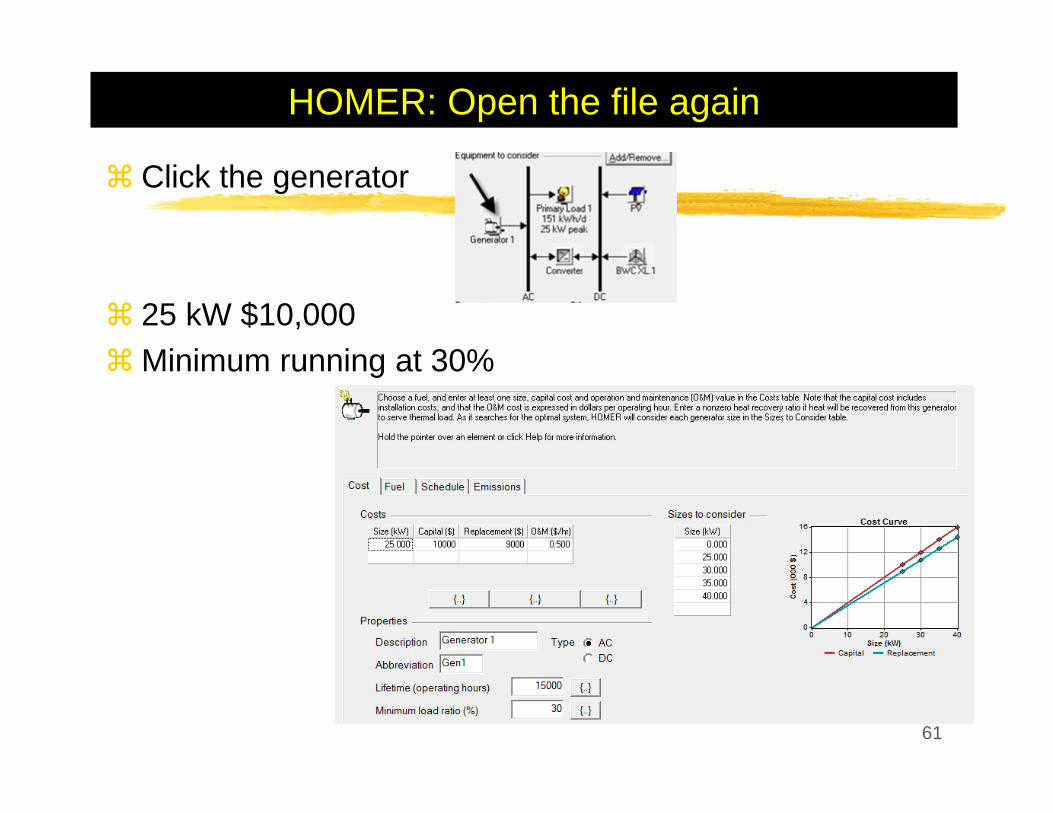
HOMER: Open the file again
Click the generator
25 kW $10,000Minimum running at 30%
61
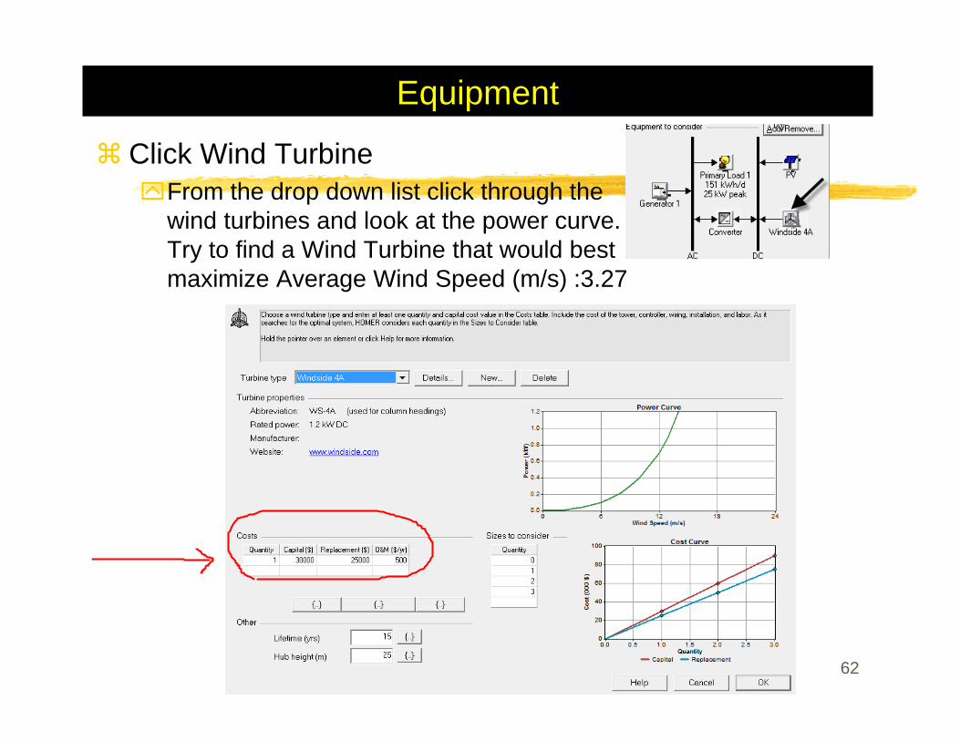
Equipment
Click Wind TurbineFrom the drop down list click through the wind turbines and look at the power curve. Try to find a Wind Turbine that would best maximize Average Wind Speed (m/s) :3.27
62
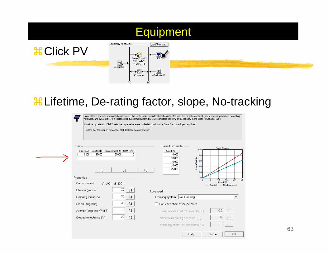
Equipment
Click PV
Lifetime, De-rating factor, slope, No-tracking
63
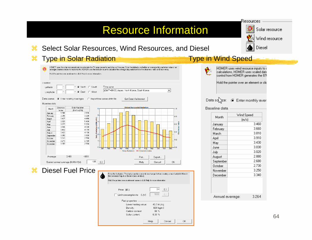
Resource InformationSelect Solar Resources, Wind Resources, and DieselType in Solar Radiation Type in Wind Speed
Diesel Fuel Price
64
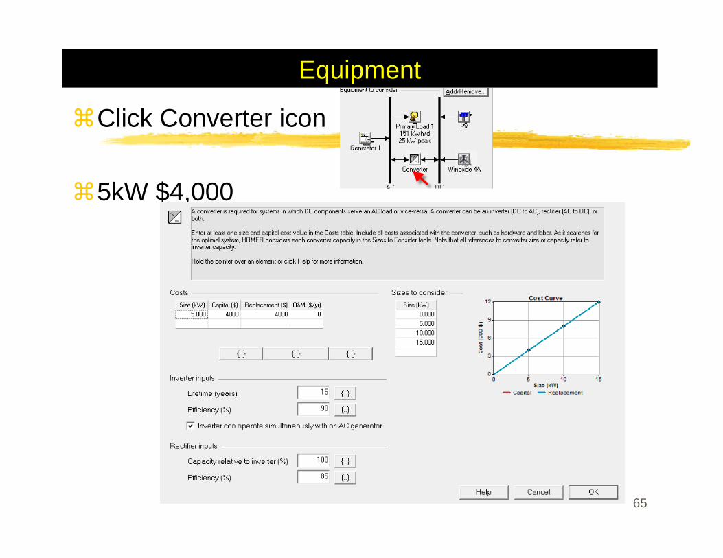
Equipment
Click Converter icon
5kW $4,000
65
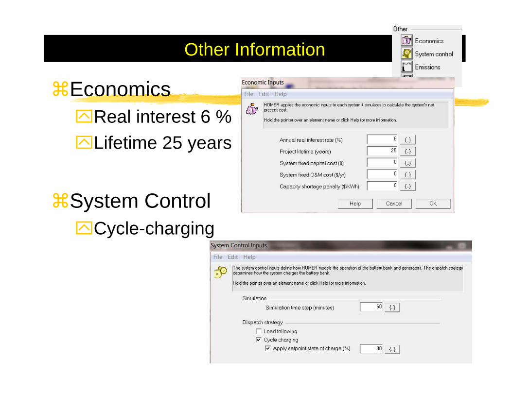
Other Information
EconomicsReal interest 6 %Lifetime 25 years
System ControlCycle-charging
66
Other Information
Emission: all 0Constraints
Operating reserve 10%Capacity shortage 0%
67
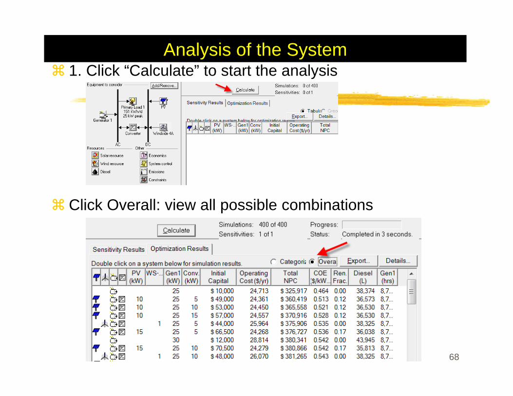
Analysis of the System1. Click “Calculate” to start the analysis
Click Overall: view all possible combinations
68
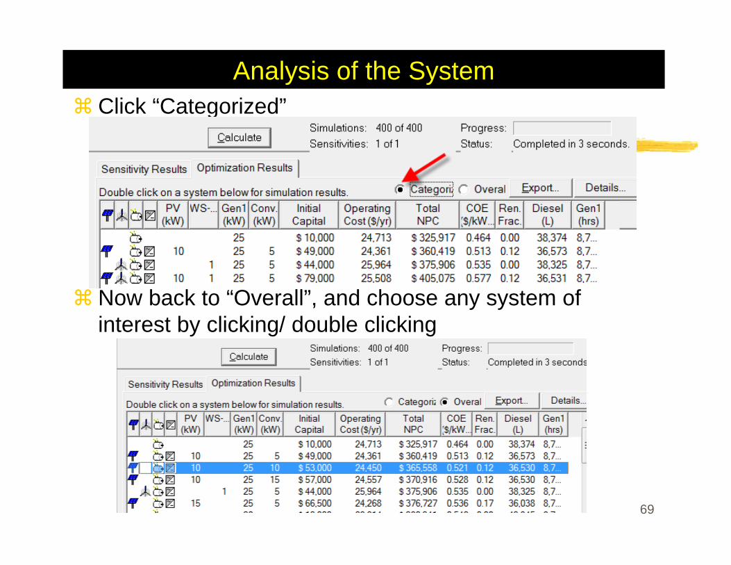
Analysis of the SystemClick “Categorized”
Now back to “Overall”, and choose any system of interest by clicking/ double clicking
69
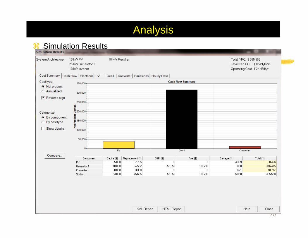
AnalysisSimulation Results
70
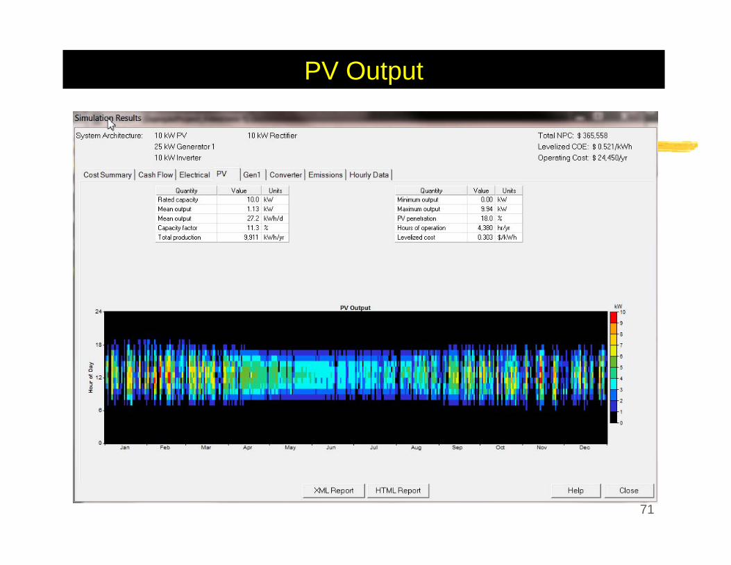
PV Output
71
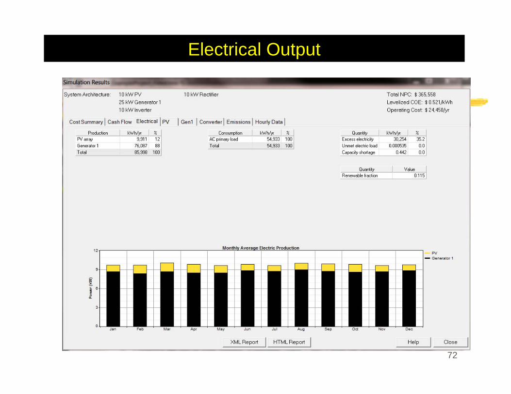
Electrical Output
72
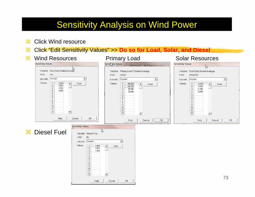
Sensitivity Analysis on Wind Power
Click Wind resourceClick “Edit Sensitivity Values” >> Do so for Load, Solar, and DieselWind Resources Primary Load Solar Resources
Diesel Fuel
73
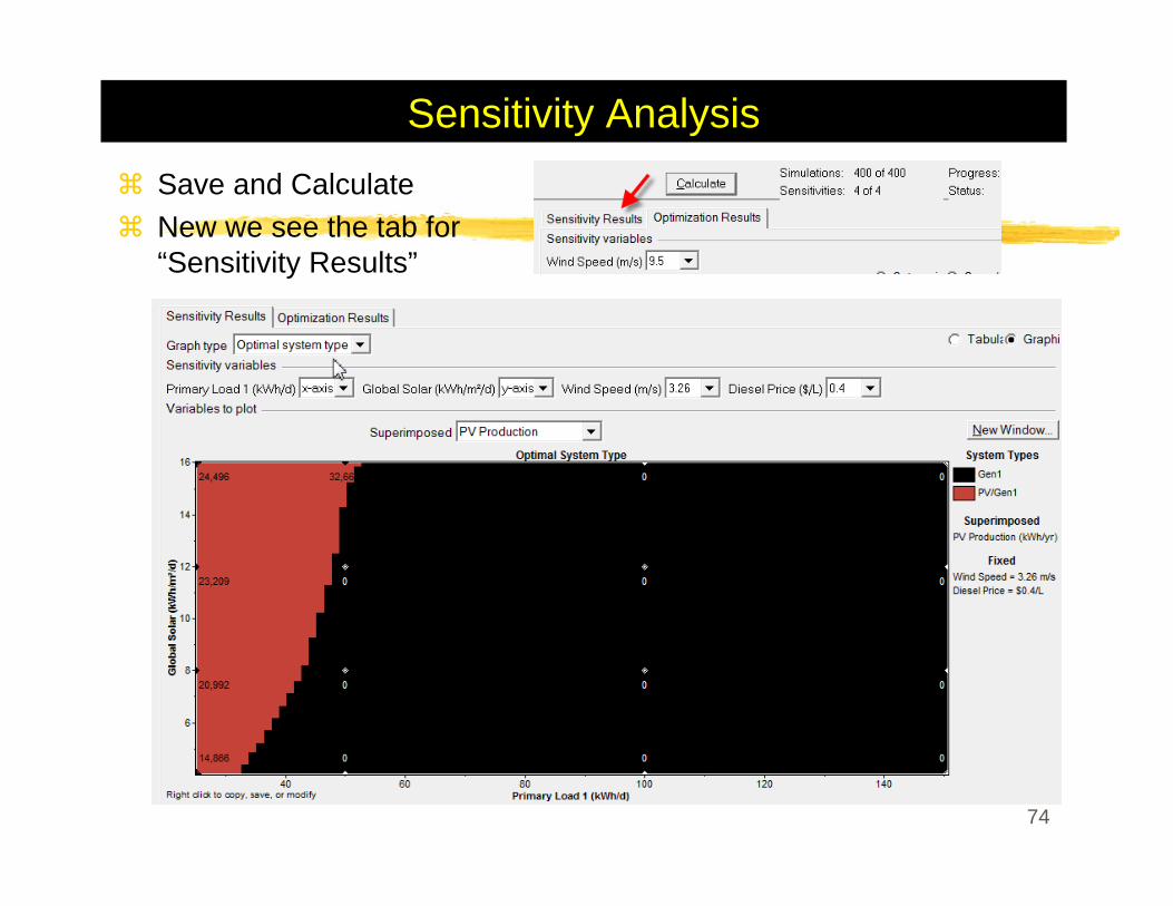
Sensitivity AnalysisSave and CalculateNew we see the tab for “Sensitivity Results”
74
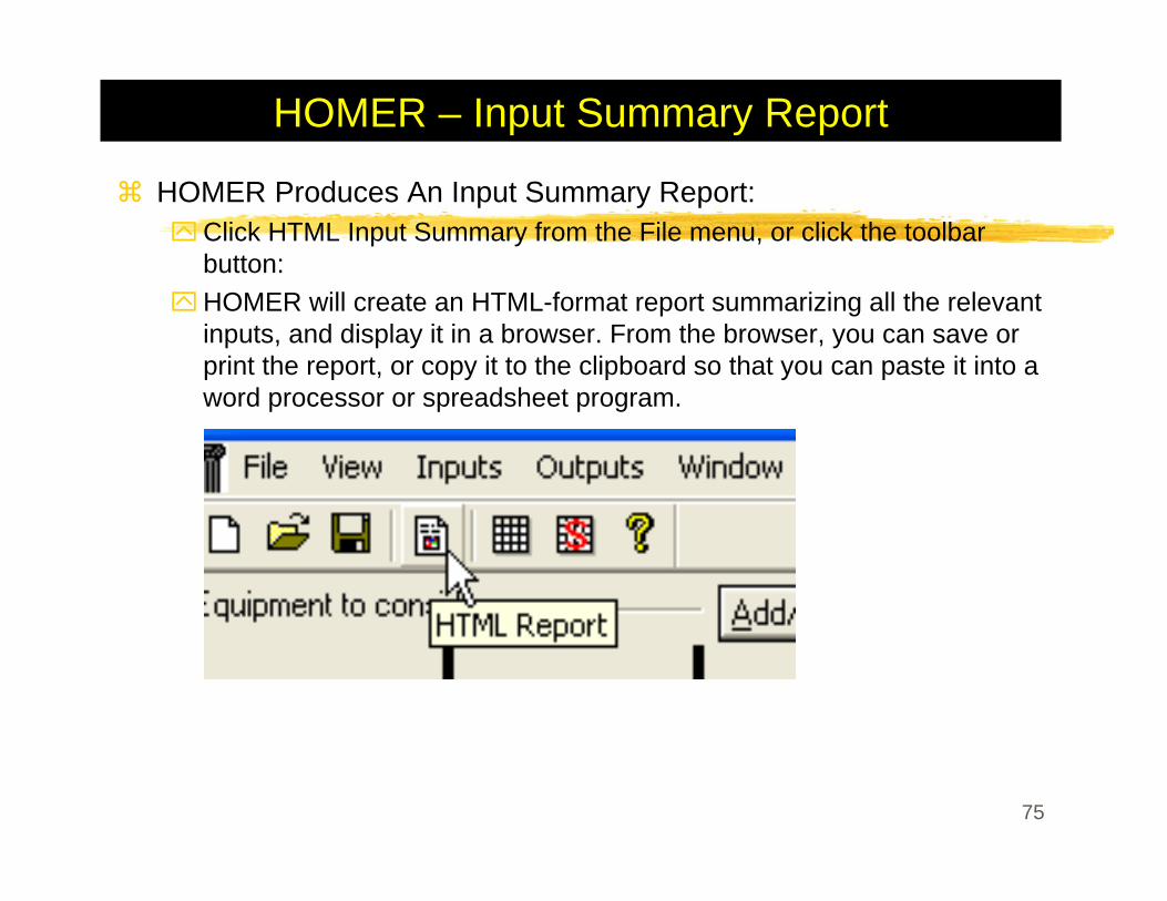
HOMER – Input Summary Report
HOMER Produces An Input Summary Report:Click HTML Input Summary from the File menu, or click the toolbar button:HOMER will create an HTML-format report summarizing all the relevant inputs, and display it in a browser. From the browser, you can save or print the report, or copy it to the clipboard so that you can paste it into a word processor or spreadsheet program.
75
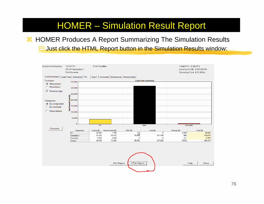
HOMER – Simulation Result ReportHOMER Produces A Report Summarizing The Simulation Results
Just click the HTML Report button in the Simulation Results window:
76
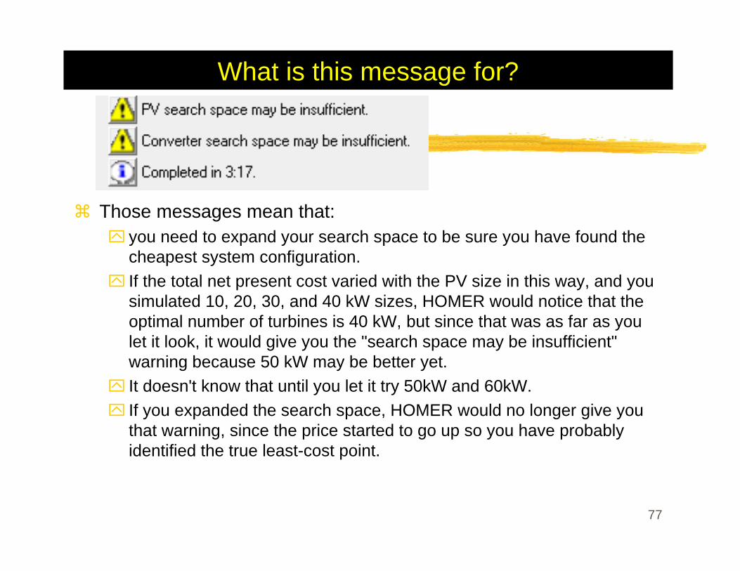
What is this message for?
Those messages mean that:you need to expand your search space to be sure you have found the cheapest system configuration. If the total net present cost varied with the PV size in this way, and you simulated 10, 20, 30, and 40 kW sizes, HOMER would notice that the optimal number of turbines is 40 kW, but since that was as far as you let it look, it would give you the "search space may be insufficient" warning because 50 kW may be better yet. It doesn't know that until you let it try 50kW and 60kW. If you expanded the search space, HOMER would no longer give you that warning, since the price started to go up so you have probably identified the true least-cost point.
77