Embed Size (px)
Citation preview

Design and optimization of vertexdetector foils by superplastic
forming
Corijn Snippe

This work is financially supported by the National Institute for SubatomicPhysics (Nikhef) in Amsterdam, and is part of the LHCb Vertex Locator pro-gram.
Samenstelling van de promotiecommissie:
voorzitter en secretaris:Prof. dr. F. Eising Universiteit Twente
promotor:Prof. dr. ir. J. Huetink Universiteit Twente
assistent promotor:Dr. ir. V.T. Meinders Universiteit Twente
leden:Prof. dr. ir. R. Akkerman Universiteit TwenteProf. dr. ing. B. van Eijk Universiteit Twente / Nikhef AmsterdamProf. dr. M.H.M. Merk Nikhef Amsterdam / VU AmsterdamDr. R.D. Wood University of Swansea, Wales (UK)
ISBN 978-90-8570-723-3
1st Printing February 2011
Keywords: superplasticity, constitutive modeling, aluminum, metal forming
This thesis was prepared with LATEX by the author and printed by WohrmannPrint Service, Zutphen, from an electronic document.
Copyright c©2011 by Q.H.C. Snippe, Leiden, The Netherlands
All rights reserved. No part of this publication may be reproduced, stored in a retrievalsystem, or transmitted in any form or by any means, electronic, mechanical, photocopying,recording or otherwise, without prior written permission of the copyright holder.
DESIGN AND OPTIMIZATION OF VERTEXDETECTOR FOILS BY SUPERPLASTIC FORMING
PROEFSCHRIFT
ter verkrijging vande graad van doctor aan de Universiteit Twente,
op gezag van de rector magnificus,prof. dr. H. Brinksma,
volgens besluit van het College voor Promotiesin het openbaar te verdedigen
op woensdag 16 maart 2011 om 15.00 uur
door
Quirin Hendrik Catherin Snippe
geboren op 21 juni 1969te Maastricht

Dit proefschrift is goedgekeurd door de promotor:
Prof. dr. ir. J. Huetink
en de assistent promotor:
Dr. ir. V.T. Meinders

Contents
Summary v
Samenvatting ix
Nomenclature xiii
1 Introduction 11.1 Vertex detection . . . . . . . . . . . . . . . . . . . . . . . . . . . . . 2
1.1.1 Basics of CP violation . . . . . . . . . . . . . . . . . . . . . . 21.1.2 Vertex reconstruction . . . . . . . . . . . . . . . . . . . . . . 4
1.2 Physical phenomena . . . . . . . . . . . . . . . . . . . . . . . . . . . 41.2.1 Radiation length . . . . . . . . . . . . . . . . . . . . . . . . . 51.2.2 Wake fields . . . . . . . . . . . . . . . . . . . . . . . . . . . . 7
1.3 LHCb Vertex Locator . . . . . . . . . . . . . . . . . . . . . . . . . . 71.3.1 Mechanical construction . . . . . . . . . . . . . . . . . . . . . 81.3.2 Properties of the RF Box . . . . . . . . . . . . . . . . . . . . 9
1.4 Problem description . . . . . . . . . . . . . . . . . . . . . . . . . . . 111.4.1 Project motivation . . . . . . . . . . . . . . . . . . . . . . . . 111.4.2 Project goal . . . . . . . . . . . . . . . . . . . . . . . . . . . . 12
1.5 Requirements . . . . . . . . . . . . . . . . . . . . . . . . . . . . . . . 131.5.1 Leak requirement . . . . . . . . . . . . . . . . . . . . . . . . . 131.5.2 Requirement on wake field suppression . . . . . . . . . . . . . 131.5.3 Mechanical requirements . . . . . . . . . . . . . . . . . . . . . 131.5.4 Radiation length . . . . . . . . . . . . . . . . . . . . . . . . . 14
1.6 Project outline . . . . . . . . . . . . . . . . . . . . . . . . . . . . . . 151.6.1 Describing superplastic behavior . . . . . . . . . . . . . . . . 151.6.2 Obtaining material behavior . . . . . . . . . . . . . . . . . . . 151.6.3 Creating the material model . . . . . . . . . . . . . . . . . . . 161.6.4 Verification of the material model . . . . . . . . . . . . . . . 171.6.5 Geometry optimization . . . . . . . . . . . . . . . . . . . . . 17
i

CONTENTS ii
2 Superplasticity 192.1 Physical mechanism of superplasticity . . . . . . . . . . . . . . . . . 20
2.1.1 Grain boundary sliding . . . . . . . . . . . . . . . . . . . . . 212.1.2 Accommodation mechanisms . . . . . . . . . . . . . . . . . . 222.1.3 Grain growth . . . . . . . . . . . . . . . . . . . . . . . . . . . 232.1.4 Cavity formation . . . . . . . . . . . . . . . . . . . . . . . . . 242.1.5 Production of superplastic materials . . . . . . . . . . . . . . 25
2.2 Superplastic materials in industry . . . . . . . . . . . . . . . . . . . . 262.2.1 Aluminum-based materials . . . . . . . . . . . . . . . . . . . 262.2.2 Titanium-based materials . . . . . . . . . . . . . . . . . . . . 272.2.3 ALNOVI-1 . . . . . . . . . . . . . . . . . . . . . . . . . . . . 27
2.3 Mechanical behavior of superplastic materials . . . . . . . . . . . . . 282.3.1 Phenomenological material behavior . . . . . . . . . . . . . . 292.3.2 Physical material behavior . . . . . . . . . . . . . . . . . . . . 32
2.4 Multiaxiality . . . . . . . . . . . . . . . . . . . . . . . . . . . . . . . 322.4.1 Flow conditions . . . . . . . . . . . . . . . . . . . . . . . . . . 332.4.2 Yield criteria . . . . . . . . . . . . . . . . . . . . . . . . . . . 342.4.3 Equivalent plastic strain and equivalent stress . . . . . . . . . 36
2.5 Hydrostatic pressure dependence . . . . . . . . . . . . . . . . . . . . 382.6 Computational (super-)plasticity . . . . . . . . . . . . . . . . . . . . 38
2.6.1 General return mapping . . . . . . . . . . . . . . . . . . . . . 392.6.2 Plane stress return mapping . . . . . . . . . . . . . . . . . . . 40
2.7 Summary and conclusions . . . . . . . . . . . . . . . . . . . . . . . . 42
3 Material experiments 433.1 Uniaxial material experiments . . . . . . . . . . . . . . . . . . . . . . 43
3.1.1 Setup of the uniaxial experiments . . . . . . . . . . . . . . . . 443.1.2 Results of the tensile tests until fracture . . . . . . . . . . . . 473.1.3 strain/vvf tensile test results . . . . . . . . . . . . . . . . . . 52
3.2 Free bulge experiments . . . . . . . . . . . . . . . . . . . . . . . . . . 563.2.1 Setup of the free bulge experiments . . . . . . . . . . . . . . . 563.2.2 Pressure control . . . . . . . . . . . . . . . . . . . . . . . . . 583.2.3 Free bulge test results . . . . . . . . . . . . . . . . . . . . . . 603.2.4 Bulge void volume fractions . . . . . . . . . . . . . . . . . . . 64
3.3 Leak tests . . . . . . . . . . . . . . . . . . . . . . . . . . . . . . . . . 673.3.1 Setup of the leak experiments . . . . . . . . . . . . . . . . . . 673.3.2 Leak test results . . . . . . . . . . . . . . . . . . . . . . . . . 67
3.4 Die bulge experiments . . . . . . . . . . . . . . . . . . . . . . . . . . 693.4.1 Friction in superplastic materials . . . . . . . . . . . . . . . . 693.4.2 Die bulge setup . . . . . . . . . . . . . . . . . . . . . . . . . . 703.4.3 Die bulge results . . . . . . . . . . . . . . . . . . . . . . . . . 72
3.5 Summary and conclusions . . . . . . . . . . . . . . . . . . . . . . . . 75

iii CONTENTS
4 Superplastic material modeling 774.1 ABAQUS material models . . . . . . . . . . . . . . . . . . . . . . . . 78
4.1.1 Plasticity models . . . . . . . . . . . . . . . . . . . . . . . . . 784.1.2 Evaluation of the classical metal plasticity model . . . . . . . 794.1.3 User-defined material model in ABAQUS . . . . . . . . . . . 82
4.2 Uniaxial model fitting . . . . . . . . . . . . . . . . . . . . . . . . . . 824.2.1 Initial flow stress . . . . . . . . . . . . . . . . . . . . . . . . . 834.2.2 Strain hardening . . . . . . . . . . . . . . . . . . . . . . . . . 844.2.3 Strain softening . . . . . . . . . . . . . . . . . . . . . . . . . . 854.2.4 Pressure dependency . . . . . . . . . . . . . . . . . . . . . . . 87
4.3 Plane stress material model . . . . . . . . . . . . . . . . . . . . . . . 884.3.1 Flow directions . . . . . . . . . . . . . . . . . . . . . . . . . . 894.3.2 Biaxial-dependent void volume fractions . . . . . . . . . . . . 90
4.4 Leak implementation . . . . . . . . . . . . . . . . . . . . . . . . . . . 914.4.1 Leak prediction . . . . . . . . . . . . . . . . . . . . . . . . . . 924.4.2 Leak description in UMAT . . . . . . . . . . . . . . . . . . . 93
4.5 UMAT procedure . . . . . . . . . . . . . . . . . . . . . . . . . . . . . 944.6 Summary and conclusions . . . . . . . . . . . . . . . . . . . . . . . . 97
5 Verification of the material model 995.1 Tensile test simulations . . . . . . . . . . . . . . . . . . . . . . . . . 99
5.1.1 Tensile test FE model . . . . . . . . . . . . . . . . . . . . . . 1005.1.2 Simulated load-displacement curves . . . . . . . . . . . . . . 1005.1.3 Simulated strain rates . . . . . . . . . . . . . . . . . . . . . . 1045.1.4 Simulated void volume fractions . . . . . . . . . . . . . . . . 104
5.2 Free bulge simulations . . . . . . . . . . . . . . . . . . . . . . . . . . 1065.2.1 Free bulge FE model . . . . . . . . . . . . . . . . . . . . . . . 1075.2.2 Free bulge simulations without backpressure . . . . . . . . . . 1085.2.3 Free bulge simulations: 30 bar backpressure . . . . . . . . . . 1115.2.4 Simulated leak rates . . . . . . . . . . . . . . . . . . . . . . . 1145.2.5 Bulge shapes . . . . . . . . . . . . . . . . . . . . . . . . . . . 115
5.3 Die bulge simulations . . . . . . . . . . . . . . . . . . . . . . . . . . . 1165.3.1 Die bulge simulations without backpressure . . . . . . . . . . 1175.3.2 Die bulge simulations with 30 bar backpressure . . . . . . . . 1185.3.3 Die bulge leak rate simulations . . . . . . . . . . . . . . . . . 118
5.4 Summary and conclusions . . . . . . . . . . . . . . . . . . . . . . . . 119
6 Optimization of the RF Foil 1216.1 Optimization theory: a brief description . . . . . . . . . . . . . . . . 122
6.1.1 Description of the optimization problem . . . . . . . . . . . . 1226.1.2 Characterization of the optimization problem . . . . . . . . . 1246.1.3 Optimization algorithms . . . . . . . . . . . . . . . . . . . . . 124
6.2 Optimization strategy . . . . . . . . . . . . . . . . . . . . . . . . . . 126

CONTENTS iv
6.2.1 Screening experiment . . . . . . . . . . . . . . . . . . . . . . 1276.2.2 Design of Experiments . . . . . . . . . . . . . . . . . . . . . . 1296.2.3 Fitting a model . . . . . . . . . . . . . . . . . . . . . . . . . . 129
6.3 RF Foil optimization goal . . . . . . . . . . . . . . . . . . . . . . . . 1326.3.1 Definition of the view factor . . . . . . . . . . . . . . . . . . . 1326.3.2 Calculation of the averaged traversed path . . . . . . . . . . . 1336.3.3 Calculation of the radiation length . . . . . . . . . . . . . . . 135
6.4 RF Foil design variables . . . . . . . . . . . . . . . . . . . . . . . . . 1366.4.1 Dimensioning of the RF Foil . . . . . . . . . . . . . . . . . . 1366.4.2 Radiation length of the simplified model . . . . . . . . . . . . 1386.4.3 Neglected design variables . . . . . . . . . . . . . . . . . . . . 139
6.5 Constraints on the RF Foil . . . . . . . . . . . . . . . . . . . . . . . 1406.5.1 Leak rate constraint . . . . . . . . . . . . . . . . . . . . . . . 1406.5.2 Mechanical constraints . . . . . . . . . . . . . . . . . . . . . . 140
6.6 Optimization results . . . . . . . . . . . . . . . . . . . . . . . . . . . 1416.6.1 Screening Design of Experiments . . . . . . . . . . . . . . . . 1426.6.2 RF Foil Design of Experiments . . . . . . . . . . . . . . . . . 1446.6.3 Optimal RF Foil design . . . . . . . . . . . . . . . . . . . . . 147
6.7 Summary and conclusions . . . . . . . . . . . . . . . . . . . . . . . . 150
7 Conclusions and recommendations 153
A Control scheme of the bulge experiments 157
B First and second derivative of the universal superplastic curve 159
C Example of an input file 161
Acknowledgments 165
Summary
The production of one of the parts in a particle detector, called the RF Foil, hasbeen a very intensive process in the past. The design and production process, whichhad a trial and error character, led eventually to an RF Foil that met the mostimportant requirement: a sufficient leak tightness value. Since these kinds of foilshave to be produced in the future, it is desirable to shorten the development stagewith a view to cost reduction. This research project investigates how this part canbe optimized with respect to the radiation length. An important limiting factorwithin this optimization process is the leak tightness of the foil. The intendedproduction method this research will investigate is superplastic forming (SPF). Onthe one hand, the goal is to use finite element calculations to predict the formingbehavior. The leak tightness of the formed foil must also be predicted within thesecalculations. On the other hand, an optimization strategy is necessary to reducethe radiation length of the RF Foil while maintaining the leak tightness.
The material that will be used throughout this research is ALNOVI-1, a materialwhich is based on AA5083. This material shows optimal superplastic propertiesat a temperature of 520 oC and an equivalent plastic strain rate of 8.3·10−4 s−1.Different types of experiments have been done to obtain as much information aspossible concerning the mechanical behavior of the material.
To determine the uniaxial behavior of the material, tensile experiments havebeen performed. The first series of tests was intended to determine the optimaltemperature at which the highest value of the equivalent plastic strains could bereached. In the second series of tensile experiments, specimens were tested untilfracture at different tensile velocities. From these tests, a high strain rate sensitivitywas measured. In the third series of tensile experiments, specimens were straineduntil a predefined value of the tensile force. The results of these tests were usedto determine the void volume fraction in the material as a function of the plasticstrain.
Free bulge experiments have been performed where circular sheets of ALNOVI-1were blown. The goal of these experiments was to study the material behavior in aplane stress situation. The application of a backpressure during forming appearedto have a positive effect on the void volume fraction evolution. In turn, this had
v

SUMMARY vi
a beneficial effect on the maximum attainable plastic strain in the material beforefailure due to a gas leak. Leak tightness experiments showed that with the appli-cation of a 30 bar backpressure, it is possible to attain much higher bulges withthe same leak rate value as bulges formed without a backpressure application.
A third type of experiment that has been done is the forming of the samecircular sheets within a die. The goal of these experiments was to investigate thefrictional behavior between ALNOVI-1 and the die material, AISI 321L. Molykotewas used as a lubricant, which is a mixture of molybdenum sulphide and graphite.The complete setup of the bulge experiments was an in-house design, where it waspossible to control the pressures on both sides of the sheet as a function of time.The shape of the pressure-time profiles was such that a predefined target plasticstrain rate in the material would not be exceeded.
The results of all experiments have been used to develop a user-defined mate-rial to be used in ABAQUS. With this phenomenological constitutive model, it ispossible to simulate the forming behavior of ALNOVI-1 as a function of a set ofparameters. These parameters describe the uniaxial behavior in terms of:
• an initial flow stress which is dependent on the equivalent plastic strain rate;
• a hardening stress due to an increasing equivalent plastic strain;
• void volume fraction evolution in the material as a function of the equivalentplastic strain. These form a bilinear relationship with each other;
• a multiplication factor (between 0 and 1) to account for the reduction instress due to the void volume fraction in the material.
The behavior in a plane stress situation is described by the Hosford flow criterionwith exponent n = 8, and taking into account the Lankford strain ratio R. Thematerial behavior also takes into account the influence of a hydrostatic pressureduring forming. The leak rate of the formed sheet can be expressed in terms of thevoid volume fraction and the resulting sheet thickness.
This constitutive model has been used to perform forming analyses of the RFFoil in view of the optimization of this foil. To perform an optimization procedure,the following ingredients are necessary to solve the problem:
• minimization of the objective function. In this project, this means a mini-mization of the radiation length of the product;
• the leak tightness is the most important constraint. Also some mechanicalconstraints were applied, such as an upper value for the stresses and elasticdeformations in the material due to an overpressure in the operating condi-tions (room temperature). A minimum value for the first natural frequencywas also applied;

vii SUMMARY
• determination of the design variables and their ranges. To limit the amountof design variables, a parameterization of the current design is necessary.
Within the range of the design variable limits, a metamodeling algorithm using theResponse Surface Methodology and Kriging was used to find the global optimum.The current RF Foil has a radiation length of 8.2% X0, the optimized RF Foilhas a radiation length of 4.6% X0. This means that the optimized RF Foil has aradiation length which is 43% lower than the radiation length of the current RFFoil. Hence, the objective of this research was met, the optimized RF Foil is abetter design than the current one.

SUMMARY viii
Samenvatting
De produktie van een van de onderdelen in een deeltjesdetector, het zogehetenRF-folie, is in het verleden een zeer arbeidsintensief proces geweest. Door het trial-and-error-karakter van het ontwerp- en produktieproces is uiteindelijk een RF-foliegeproduceerd dat aan de belangrijkste eis voldoet: een goede lekdichtheid. In hetgeval er in de toekomst dit soort folies geproduceerd moeten worden, moet dit ont-wikkelingstraject verkort worden met het oog op kostenbesparing. In dit projectwordt onderzocht hoe dit onderdeel geoptimaliseerd kan worden met betrekkingtot de stralingslengte, waarbij de lekdichtheid een belangrijke limiterende factoris. De beoogde produktiemethode die hier wordt onderzocht is die van het super-plastisch vervormen (SPF). Doel is enerzijds om het vervormingsgedrag te kunnenvoorspellen aan de hand van eindige elementenanalyses en daarmee ook een voor-spelling te kunnen doen omtrent de lekdichtheid van het gevormde folie. Anderzijdsis het de bedoeling een optimalisatiestrategie te ontwikkelen om de stralingslengtevan het RF-folie te verlagen met behoud van de lekdichtheid.
Het materiaal dat gebruikt wordt voor dit onderzoek is ALNOVI-1, een mate-riaal gebaseerd op AA5083. Dit materiaal vertoont optimale superplastische eigen-schappen bij een temperatuur van 520 oC en een equivalente plastische reksnelheidvan 8.3·10−4 s−1. Verschillende typen experimenten zijn uitgevoerd om een zovolledig mogelijk beeld te krijgen van het mechanisch gedrag van dit materiaal.
Om het uniaxiale gedrag van het materiaal te bepalen zijn trekproeven uitgevoerd.De eerste serie proeven hiervan had als doel om de temperatuur te bepalen waarbijde hoogste plastische rekken haalbaar zijn alvorens het materiaal faalt door breuk.Bij de tweede serie trekproeven zijn proefstukken bij deze optimale temperatuurgetest tot breuk, bij verschillende treksnelheden. Uit deze proeven bleek onderandere een hoge mate van reksnelheidsafhankelijkheid. De derde serie trekproevenbestond uit experimenten waarbij de proefstukken werden getrokken tot een voorafingestelde waarde van de trekkracht. Aan de hand van deze proeven is de matevan holtevorming in het materiaal bepaald als functie van de plastische rek.
Blaasvormtesten zijn uitgevoerd waarbij cirkelvormige plaatjes ALNOVI-1 on-der overdruk tot een bolle vorm zijn geblazen. Deze experimenten hadden alsdoel om het materiaalgedrag te bestuderen onder een vlakspanningstoestand. Het
ix

SAMENVATTING x
aanleggen van een hydrostatische druk tijdens het vervormingsproces bleek eengunstige uitwerking te hebben op het holtevormingsgedrag, en daarmee op de max-imaal haalbare plastische rek in het materiaal alvorens falen optreedt in de vormvan een gaslek. Gasdichtheidsproeven hebben aangetoond dat onder invloed vaneen hydrostatische druk van 30 bar het mogelijk is om blaasvormen te maken dieeen stuk verder vervormd zijn bij eenzelfde lekdichtheid dan zonder deze druk.
Een derde type experiment dat is uitgevoerd is het blaasvormen van dezelfdecirkelvormige plaatjes in een mal. Deze proeven hadden als doel om het wrijvings-gedrag te onderzoeken tussen ALNOVI-1 en de mal, gemaakt van AISI 321L. Hetgebruikte smeermiddel om deze wrijving te bereiken was Molykote, een mengselvan molybdeensulfide en grafiet.
Voor alle blaastesten is gebruik gemaakt van een zelf ontworpen proefopstellingwaarbij het mogelijk was om de vervormingsdruk op de plaat te varieren als functievan de tijd. De druk-tijdprofielen hiervoor waren zodanig dat tijdens dit vervor-mingsproces een vooraf bepaald doelwaarde voor de equivalente plastische reksnel-heid nergens in het materiaal werd overschreden.
De resultaten van alle proeven zijn verwerkt in een User-defined material modelin ABAQUS. Met dit fenomenologische materiaalmodel is het mogelijk om hetvervormingsgedrag van ALNOVI-1 te simuleren als functie van een set parameters.Deze parameters beschrijven het uniaxiale gedrag in termen van:
• een initiele vloeispanning die afhankelijk is van de equivalente plastische rek-snelheid;
• een spanningstoename als gevolg van een toenemende equivalente plastischerek;
• holtevorming in het materiaal als functie van de equivalente plastische rek.Dit is een bilineaire relatie;
• een vermenigvuldigingsfactor (tussen 0 en 1) die de spanningsreductie aangeeftals gevolg van holtevorming in het materiaal.
Het gedrag onder een vlakspanningstoestand is beschreven middels het Hosfordvloeicriterium met exponent n = 8, met inachtneming van de rekverhouding R.Tevens is het gedrag beschreven onder invloed van een hydrostatische druk. Delekdichtheid van het materiaal kan worden uitgedrukt in termen van de holtevormingen de resulterende dikte van de plaat.
Dit materiaalmodel is gebruikt om vervormingsanalyses te doen met betrekkingtot het RF-folie met het oog op optimalisatie van dit folie. Om een optimalisatiepro-cedure uit te voeren is het probleem beschreven in de volgende termen:
• minimalisatie van de doelfunctie, in dit geval houdt dit een minimalisatie vande stralingslengte van het produkt in;

xi SAMENVATTING
• de lekdichtheid is de belangrijkste randvoorwaarde. Daarnaast zijn mecha-nische eigenschappen vereist, zoals een grenswaarde voor de spanningen enelastische vervormingen in het materiaal als gevolg van een overdruk op hetfolie in de gebruiksomstandigheden (kamertemperatuur). Tevens is een mi-nimale waarde vereist voor de eerste eigenfrequentie van het folie;
• aangeven van de ontwerpvariabelen met elk hun bereik. Hiervoor is een para-metrisatie van het huidige ontwerp noodzakelijk.
Binnen het bereik van de ontwerpvariabelen wordt een metamodelleringsalgoritme(gebruikmakend van de Response Surface Methodolgy en Kriging) gebruikt omhet globale optimum te vinden. Het huidige folie heeft een stralingslengte van8.2% X0, het geoptimaliseerde RF-folie heeft een stralingslengte van 4.6% X0. Ditbetekent dat het geoptimaliseerde folie een stralingslengte heeft die 43% lager ligtdan die van het huidige folie. Daarmee kan dus gezegd worden dat het doel van ditonderzoek is behaald, het geoptimaliseerde RF-folie is beter dan het huidige folie.

SAMENVATTING xii

Nomenclature
Roman symbols
A atomic weightAi area of surface iC elasticity tensor (second-order)4C elasticity tensor (fourth-order)D rate-of-deformation tensord grain size (Chapter 2)d displacementdc channel diameterE Young’s modulusF forceFj view factorFobj objective function valueG shear modulusgi inequality constraint ihj equality constraint jI1, I2 stress invariantsk Boltzmann constantks stress concentration factorL leak ratel (effective/channel) lengthM grain boundary mobilitym strain rate sensitivityNA Avogadro constantn Hosford exponentp pressureph hydrostatic pressureQ fluid flow rateQn quality factorRs shunt impedanceR Lankford strain ratio
xiii

NOMENCLATURE xiv
R0, R45, R90 direction dependent strain ratiosR average strain ratioΔR strain ratio sensitivityR2 coefficient of multiple determinationR2
adj adjusted coefficient of multiple determinationr vector of residualsS distancesij deviatoric stress componentss deviatoric stress tensorT temperaturet thicknessts time (in seconds)t average traversed pathv drawing velocityX0 radiation lengthW void aspect ratioZ atomic number
Greek symbols
α electromagnetic interaction constantγxy engineering shear strainε strain vectorε strain rate vectorεp equivalent plastic strain˙εp equivalent plastic strain rateεtr transition strainη dynamic viscosityκ loss factorλ stretchλ plastic multiplierν Poisson’s ratioξ, ξv void volume fractionξa void area fractionΣh hydrostatic stressσe equivalent stressσf macroscopic flow stressσm matrix material yield stressσsurf grain boundary energy densityσy yield stressσ1, σ2, σ3 principal stress componentsΔσ saturation stress

xv NOMENCLATURE
σ stress vectorσtr trial stress vectorτmax maximum shear stressφ flow function valueΩ vacancy volumeω radial frequency
Abbreviations
ARB Accumulative Roll BondingBP BackpressureCERN European Organization for Nuclear ResearchCGBS Cooperative Grain Boundary SlidingCP Charge ParityCTE Coefficient of Thermal ExpansionDOE Design of ExperimentsECA Equal Channel Angular ExtrusionEM Electro-MagneticFE(M) Finite Element (Method)GBS Grain Boundary SlidingGEANT GEometry ANd TrackingLHC Large Hadron ColliderLHCb Large Hadron Collider B detectorRF Radio FrequencyRMSE Root Mean Square ErrorRSM Response Surface MethodologySPF Superplastic FormingUMAT User-Defined Material ModelVeLo Vertex Locator
1. Introduction
At the end of 2009, the Large Hadron Collider (LHC) particle accelerator at theEuropean Organization for Nuclear Research (CERN) in Geneva was started up,being the world’s largest scientific experiment at that moment. In the upcomingyears research will be carried out in the field of subatomic physics, involving highprecision particle trajectory measurements. This scientific experiment aims at abetter understanding of the subatomic structure of matter and its interactions.
One of the four detectors positioned in the accelerator is the LHCb experiment.The main goal of this experiment is to understand why there exists a large asym-metry between the existence of matter and antimatter. A necessary ingredient toexplain this asymmetry is the existence of so-called CP violation, where CP standsfor charge and parity. To do this, LHCb aims at measuring the decay time ofparticles which show a relatively high amount of CP violation, so-called B mesonsand anti-B mesons. These are unstable particles that are, among others, productsof proton-proton collisions within the accelerator.
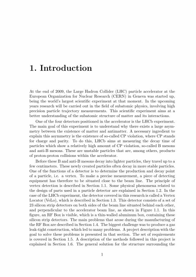
Before these B and anti-B mesons decay into lighter particles, they travel up to afew centimeters. These newly created particles often decay in more stable particles.One of the functions of a detector is to determine the production and decay pointof a particle, i.e. a vertex. To make a precise measurement, a piece of detectingequipment has therefore to be situated close to the beam line. The principle ofvertex detection is described in Section 1.1. Some physical phenomena related tothe design of parts used in a particle detector are explained in Section 1.2. In thecase of the LHCb experiment, the detector covered in this research is called a VertexLocator (VeLo), which is described in Section 1.3. This detector consists of a set of23 silicon strip detectors on both sides of the beam line situated behind each other,and perpendicular to the accelerator beam line, as shown in Figure 1.1. In thisfigure, an RF Box is visible, which is a thin-walled aluminum box, containing thesesilicon strip detectors. The main problems that arose during the manufacturing ofthe RF Box are described in Section 1.4. The biggest challenge was to produce a gasleak-tight construction, which led to many problems. A project description with thegoal to solve these problems is presented in that section. The set of requirementsis covered in Section 1.5. A description of the methods followed in this project isexplained in Section 1.6. The general solution for the structure surrounding the
1
1 Introduction 2
Silicon strip detectorsVacuum tank
RF Box
Beam line
Figure 1.1: Placement of the silicon strip detectors in a vacuum tank, surrounding theaccelerator beam.
detectors is called an RF Shield, RF standing for Radio Frequency. The solutionchosen in the current design is a box, called the (already mentioned) RF Box. Thetop sheet of this box, which is closest to the beam line, is the RF Foil.
1.1 Vertex detection
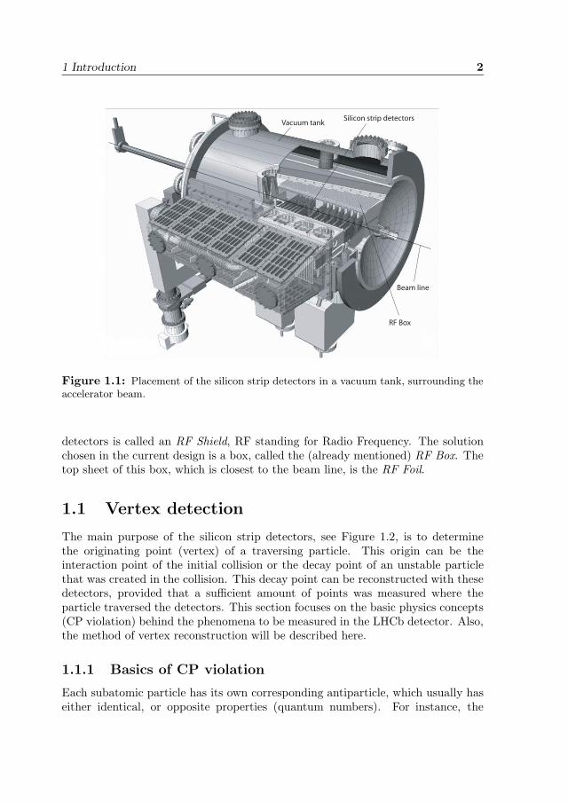
The main purpose of the silicon strip detectors, see Figure 1.2, is to determinethe originating point (vertex) of a traversing particle. This origin can be theinteraction point of the initial collision or the decay point of an unstable particlethat was created in the collision. This decay point can be reconstructed with thesedetectors, provided that a sufficient amount of points was measured where theparticle traversed the detectors. This section focuses on the basic physics concepts(CP violation) behind the phenomena to be measured in the LHCb detector. Also,the method of vertex reconstruction will be described here.
1.1.1 Basics of CP violation
Each subatomic particle has its own corresponding antiparticle, which usually haseither identical, or opposite properties (quantum numbers). For instance, the
3 1.1 Vertex detection
RF Box
RF Foil
Silicon strip detector
Beam line
Figure 1.2: Placement of one row of silicon strip detectors within the RF Box.
charge of the antiparticle is always the opposite of the charge of the correspondingparticle, but the mass of both particle and antiparticle is the same. The antiparti-cle of the electron, which has one unit negative charge, has one unit positive chargeand is called an anti-electron or positron, but both have the same mass. It is to beexpected that both particle and antiparticle also obey either the same or mirroredphysical laws.
A mirrored particle is called parity or P transformed with respect to the originalparticle. The transformation involves the change of a right-handed coordinatesystem into a left handed one. This can be imagined by mirroring a particle twotimes: a vertical-mirror deflection followed by a top-bottom switch. A charge or Ctransformation changes the sign of the electric charge of the particle. If both C andP transformations act onto a particle, then this would lead to the correspondingantiparticle, which should have identical properties to those of the particle.
In the 1960s, experiments with particles called kaons showed that occasionallyparticles behave differently than their CP mirrored particles, the anti-kaons. Bothparticles can decay the same way in two other particles, but experiments showthat the probability for these kaons and anti-kaons to decay were slightly different.This meant that particles and antiparticles can behave or decay differently. Thisphenomenon is called CP violation, see for instance [84], and this is thought tobe the main reason why there is an abundance of matter in the universe above
1 Introduction 4
antimatter.To find the underlying mechanism for this phenomenon to occur, experiments
will be performed with the LHCb detector which studies the CP violation in B-mesons. These particles are largely produced in proton-proton colliders, such asthe LHC, and it is expected that these mesons show a larger CP violation effectthan kaons. By reconstructing the decay point of the B-mesons and its antiparticles,further proof and quantization of CP violation is then possible. The reconstructionof these decay points is done using the LHCb Vertex Locator.
1.1.2 Vertex reconstruction
In order to trace the particles coming from a collision between two acceleratedparticles, a detector has to be placed around the interaction point. A particledetector generally consists of a layered structure of different kinds of detectors,since it is not possible to detect all sorts of particles with one single detector. Eachlayer has its own characteristics and measurement accuracy, which is not onlyable to distinguish the particle type, but can also be used to measure the particlemomentum and/or charge.
In semiconductor materials like silicon, the energy required to create anelectron-hole pair is very low, about 3 eV. Semiconductor detectors are typicallybuilt out of 20 to 50 μm wide and 300 μm thin silicon strips or pixels bonded on ahybrid (a low thickness avoids multiple scattering). Traversing elementary chargedparticles of high energy can easily create tens of thousands electron-hole pairs toobtain a signal. A stack of silicon strip detectors can then be used to determinethe trajectories of charged particles to a high degree of accuracy. Therefore theyare used to detect whether a particle originates from the initial collision point orfrom a secondary point, (i.e. a vertex, depending on other particles emerging fromthe same point which are measured at the same time). This secondary point canbe the originating point of a decay product, and is then a measure for the lifetimeof the decayed particle.
1.2 Physical phenomena
Besides the physical phenomenon of CP violation, which has already been dis-cussed, two other phenomena will be covered here, because they both have aninfluence on the design of the RF Shield. The first one is the so-called multiplescattering, which is related to the fact that charged particles deviate from theirtrajectory inside a material, because of the electro-magnetic interaction with thecharged particles in this material. All these summed interactions influence thetrajectory of the traveling particle through the detector, which in its turn influ-ences the physical particle measurement in terms of kinetic energy and position.

5 1.2 Physical phenomena
The amount of energy loss is expressed in a term called radiation length and is amaterial and geometrical property.
The other physical aspect which influences the design of the RF Shield is wakefield suppression. In the LHC, protons are accelerated; a consequence is that inthe wall of the beam pipe, particles with opposite charge (electrons) will followthe accelerated proton bunches. If this cloud of mirror charge electrons cannotfollow the corresponding proton bunch closely enough, the next proton bunch willbe influenced, thereby losing part of its energy. This can happen if the electronscannot travel straight ahead through the beam pipe, but are deviated from theirpath. Deviated charged particles give off radiation; this is called a wake field.
1.2.1 Radiation length
In order to be detected, an object must leave a trace inside matter as proof ofits presence. This means that this particle must leave some energy in its wake,decreasing the kinetic energy of the particle itself. To accurately measure all thedesired properties of this particle, the deposited energy must be low (or predictable)compared to its own energy in order not to disturb the particle trajectory too much.At very high energies, above 100 MeV (which is the case in LHC), charged particlestraveling in matter lose energy. These particles are accelerated and deceleratedin matter because of the electromagnetic interaction with the atomic magneticfields. This energy loss as function of the traveling length through the matter ispredictable, and can therefore be corrected for within the measurements. Electrons,which are very light charged particles, suffer in addition from a phenomenon calledbremsstrahlung (’brake radiation’). These electrons also give off energy by radiatingelectromagnetic waves as bremsstrahlung photons.
Bremsstrahlung is not predictable. When a charged particle travels throughmatter, the trajectory will deviate from the original trajectory, because chargedparticles inside this matter will disturb the traversing charged particle. Each timethis charged particle passes a charged particle inside the traversed matter, singlescattering will occur. The sum of all the single scatterings inside the material isthe amount of multiple scattering. Therefore, the total amount of traversed mattershould be as low as possible. Both the effects of bremsstrahlung and multiplescattering are covered in the radiation length value of a material.
This radiation length is dependent on some properties of the material and of theradius of the electron, re, having a value of 2.818 fm. The magnetic fields inside thematerial are dependent on the atomic number Z, which is an indicator of charge,and the atomic weight A, which is an indicator of volume. Also the couplingconstant for the electromagnetic interaction, α (equal to 1/137), is involved in thisrelationship. There are many empirical laws derived from these basic properties,but a few empirical formulas, developed by data fit, are common. The one which
1 Introduction 6
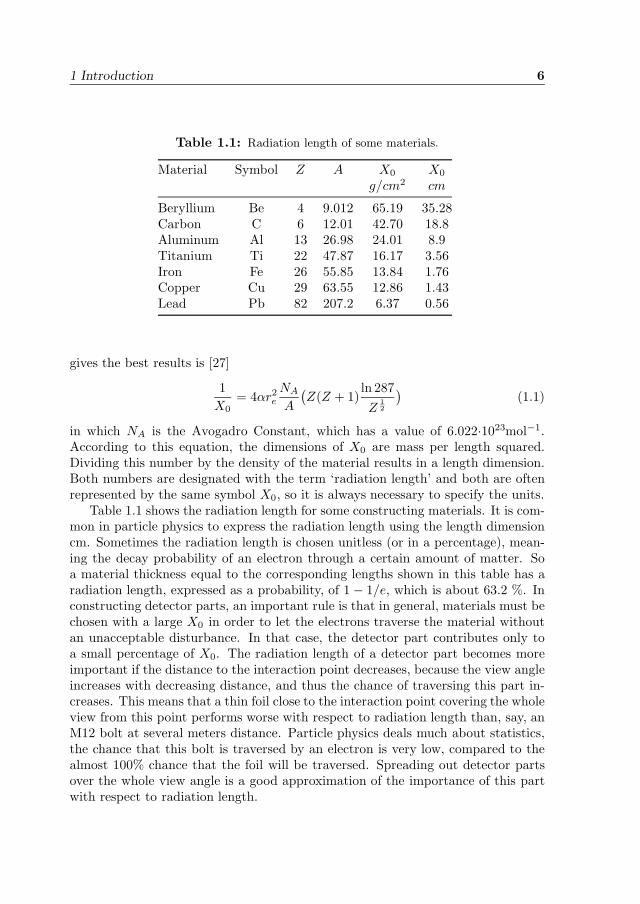
Table 1.1: Radiation length of some materials.
Material Symbol Z A X0 X0
g/cm2 cm
Beryllium Be 4 9.012 65.19 35.28Carbon C 6 12.01 42.70 18.8Aluminum Al 13 26.98 24.01 8.9Titanium Ti 22 47.87 16.17 3.56Iron Fe 26 55.85 13.84 1.76Copper Cu 29 63.55 12.86 1.43Lead Pb 82 207.2 6.37 0.56
gives the best results is [27]
1X0
= 4αr2e
NA
A
(Z(Z + 1)
ln 287Z
12
)(1.1)
in which NA is the Avogadro Constant, which has a value of 6.022·1023mol−1.According to this equation, the dimensions of X0 are mass per length squared.Dividing this number by the density of the material results in a length dimension.Both numbers are designated with the term ‘radiation length’ and both are oftenrepresented by the same symbol X0, so it is always necessary to specify the units.
Table 1.1 shows the radiation length for some constructing materials. It is com-mon in particle physics to express the radiation length using the length dimensioncm. Sometimes the radiation length is chosen unitless (or in a percentage), mean-ing the decay probability of an electron through a certain amount of matter. Soa material thickness equal to the corresponding lengths shown in this table has aradiation length, expressed as a probability, of 1 − 1/e, which is about 63.2 %. Inconstructing detector parts, an important rule is that in general, materials must bechosen with a large X0 in order to let the electrons traverse the material withoutan unacceptable disturbance. In that case, the detector part contributes only toa small percentage of X0. The radiation length of a detector part becomes moreimportant if the distance to the interaction point decreases, because the view angleincreases with decreasing distance, and thus the chance of traversing this part in-creases. This means that a thin foil close to the interaction point covering the wholeview from this point performs worse with respect to radiation length than, say, anM12 bolt at several meters distance. Particle physics deals much about statistics,the chance that this bolt is traversed by an electron is very low, compared to thealmost 100% chance that the foil will be traversed. Spreading out detector partsover the whole view angle is a good approximation of the importance of this partwith respect to radiation length.
7 1.3 LHCb Vertex Locator
1.2.2 Wake fields
If a bunch of charged particles moves along a piece of material, mirror currentswith the opposite charge will start to appear in this material. This is constantlythe case in the beam pipe of LHC. These mirror currents move just behind thebunch, but will not influence the next bunch of particles. However, if geometricalobstacles are present, the mirror current cannot follow the original particle bunch,because the path to travel will become longer with each deviation from the beampath [6]. These mirror currents then create electro-magnetic fields, called wakefields, which have to be suppressed because of two main reasons:
• wake fields can damage the environment by heating;
• wake fields degrade the next bunches in the beam, because of the generatedEM fields.
For these reasons, besides some other reasons not dealing with wake field suppres-sion, detector modules may not be placed inside the beam vacuum.
The energy of a wake field is the same as the energy loss of the beam, which isexpressed by using a longitudinal loss factor κ‖. This factor is dependent on thedistance from the beam to the surrounding structure and on the charge distributionin the bunch, and has to be solved numerically in case of obstacles. This loss factoris then used in an expression which can be interpreted as an extra impedance onthe bunch, the shunt impedance Rs, expressed in the frequency domain [7]
Rs = 2κ‖nQn
ωnΩ (1.2)
in which κ‖n is the loss factor for eigenmode n with frequency ωn and Qn is aquality factor dependent on the geometry of the cavity.
1.3 LHCb Vertex Locator
The main function of the structural parts in a particle detector is to hold allthe detection devices in place and keep them in good condition. To avoid internalstresses as much as possible, it is frequently desirable to ensure that that supportingconstructions are kinematically supported, i.e. there are no redundant degrees offreedom in the structure. This is not only to make up for manufacturing tolerances,but also to take into account occasional temperature differences as time progressesduring operation.
The Vertex Locator in the LHCb detector consists of two rows of 23 silicon stripdetectors, each row situated on either side of the accelerator beam. These rows ofstrip detectors are placed within a vacuum tank, as was shown in Figure 1.1.

1 Introduction 8
The vacuum space in which the detector rows are situated is separated fromthe accelerator beam vacuum by means of a thin aluminum shield, the RF Shield.This shield has three main functions:
• it protects the beam pipe vacuum against pollution from the detector vacuum,caused by outgassing of the detector hybrids;
• it serves as a wake field suppressor, see Section 1.2.2;
• it protects the sensors against the high EM frequency in the RF spectrum atwhich the proton bunches pass by (40 MHz), hence the abbreviation ’RF’ inthe names ’RF Shield’, ’RF Box’ and ’RF Foil’.
1.3.1 Mechanical construction
A picture of the two RF Boxes is shown in Figure 1.3(a) [40]. In the final setupeach box will contain one row of 23 silicon strip detectors. The two rows are shiftedwith respect to each other in the direction of the beam, so these rows can then besituated such that the detectors partly overlap, see Figure 1.3(b) for a cross sectionof this setup. The two RF Boxes were designed in a way that they each cover onerow of detectors, hence their wave-like structure. The reason for overlapping of thedetectors is that in this way all (charged) particles emerging from a collision willbe detected. In addition, the overlapping detectors provide a means to determinetheir relative alignment.
(a) (b)
particle tracksilicon detector
top RF Foil
bottom RF Foil
Figure 1.3: (a) Two RF Boxes (left and right) which have to cover both rows of silicondetectors; (b) Cross section view showing the necessity of the wave-like structure of theRF Boxes.
The RF Boxes are made from an aluminum based on AA 5083, an Al-Mg alloy.Sheets of this material that were used for the manufacturing of the RF Foil, had

9 1.3 LHCb Vertex Locator
an initial thickness of 0.3 mm. These sheets were heated up to a temperaturebetween 315 and 350 oC, then gas pressure was applied such that each 15 minutesthe pressure was instantaneously increased by 1 bar, until a value of 12 bar wasreached. Subsequently, the pressure was increased instantaneously until a value of20 bar, which was held for one hour before the formed sheet was taken out of thedie.
Besides the top foil, the side foils were also manufactured in this way. Theparticles to be measured always cross the top foil first one ore more times beforethe detectors are hit. This means that the top foil construction is critical in terms ofradiation length. The side walls of the RF Box are only hit just after the detectorsare hit, so the construction in terms of radiation length is less critical. The fivefoils are connected to each other by a welding procedure.
1.3.2 Properties of the RF Box
The dimensions of the RF Box are presented in Figure 1.4 [40]. The RF Foil, whichis the top sheet of the RF Box, measures 1120 by 200 mm.
1175
270
270
Figure 1.4: Dimensioning of the RF Box.
Two main properties of the RF Box, and in particular the RF Foil, are definedin terms of the wake field suppression and the radiation length. Wake fields aresuppressed by the Toblerone-like shape of the RF Foil, the corrugation depth ofthe wave structure is less than 20 mm [8], which is known to result in a sufficientwake field suppression.
1 Introduction 10
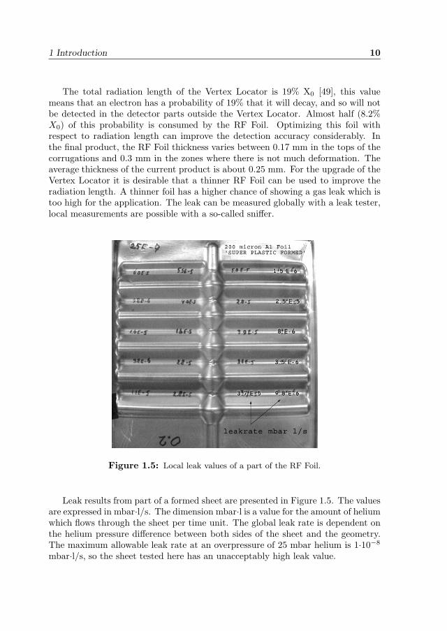
The total radiation length of the Vertex Locator is 19% X0 [49], this valuemeans that an electron has a probability of 19% that it will decay, and so will notbe detected in the detector parts outside the Vertex Locator. Almost half (8.2%X0) of this probability is consumed by the RF Foil. Optimizing this foil withrespect to radiation length can improve the detection accuracy considerably. Inthe final product, the RF Foil thickness varies between 0.17 mm in the tops of thecorrugations and 0.3 mm in the zones where there is not much deformation. Theaverage thickness of the current product is about 0.25 mm. For the upgrade of theVertex Locator it is desirable that a thinner RF Foil can be used to improve theradiation length. A thinner foil has a higher chance of showing a gas leak which istoo high for the application. The leak can be measured globally with a leak tester,local measurements are possible with a so-called sniffer.
Figure 1.5: Local leak values of a part of the RF Foil.
Leak results from part of a formed sheet are presented in Figure 1.5. The valuesare expressed in mbar·l/s. The dimension mbar·l is a value for the amount of heliumwhich flows through the sheet per time unit. The global leak rate is dependent onthe helium pressure difference between both sides of the sheet and the geometry.The maximum allowable leak rate at an overpressure of 25 mbar helium is 1·10−8
mbar·l/s, so the sheet tested here has an unacceptably high leak value.
11 1.4 Problem description
In normal operation conditions, the pressure difference between the two sidesof the RF Foil is less than 1 mbar. Under the load of this pressure difference, thedeflection of the RF Foil may not exceed 1 mm, since both RF Foils may not comeinto contact with each other. It is calculated that the shield will show irreversibledeformation at a pressure difference of 17 mbar [14], which is considered sufficientfor this design. It was tested that in case of an emergency, the maximum pressuredifference will be 6 mbar, before an overpressure valve opens. This pressure onlyoccurs in case of a sudden air inlet into the RF Box. Further, it is of crucialimportance that the first natural frequency of the RF Box is high enough to avoidresonance at external transient inputs from moving parts, such as rotating partsof a pump. The first natural frequency of the current RF Box is calculated at 107Hz [14], which is high enough to avoid resonating with the input frequencies. It isa general rule that the first resonance frequency is always higher than 50 Hz.
1.4 Problem description
Together with the Vertex Locator, an RF Box is integrated which separates thevacuum, in which the silicon detectors are present, from the beam pipe vacuum.This shield serves two main purposes. Firstly, a boundary is necessary between thetwo vacua to prevent the occurrence of outgassing from the silicon detectors intothe beam pipe vacuum. A vitally important point that has to be mentioned in thiscontext is that this shield has to prevent a gas leak between these two vacua fromarising under any circumstances whatsoever. Secondly, this shield should suppresswake fields as much as possible, as was explained in Section 1.2.2. It is importantthat the electric conductance of the beam pipe itself may not be interrupted, thisshield therefore also has the function of a surrogate beam pipe section.
1.4.1 Project motivation
The shield is manufactured by means of Hot Gas Forming, a process where a heatedthin sheet of aluminum is pressed into a one-sided die by means of an increasing gaspressure. This has been mainly a lengthy trial-and-error process for several yearsin terms of material type, forming temperature, and gas pressure. This processresulted in a product which more or less meets the requirement of leak-tightness.The shield has been optimized mainly on the run, solving forming problems on thistrial-and-error basis.
Because the shield is positioned very close to the interaction point, it has a verywide view angle, almost 100%, as seen from this point. This means that this shieldconsumes a major part of the radiation length of the LHCb detector, a phenomenonwhich was explained in Section 1.2.1. In summary, optimizing with respect to thisquantity means in general a mass minimization problem.
1 Introduction 12
Accurate vertex detection is expected to be necessary also in future detectors,requiring a similar protection shield. It would then be advantageous if the de-sign process can be reduced significantly by simulating the forming process of theshield together with an optimization procedure with respect to the radiation lengthquantity.
It is known that a forming process called Superplastic Forming (SPF) can beadvantageous in cases of low series production where high plastic strains are tobe expected. Since only two RF Shields are necessary inside the particle detector,superplastic forming seems a highly attractive manufacturing method for theseshields. It is not only to be expected that in the future more of these shields are tobe made for future particle detectors, but also for an upgrade of the LHCb VertexLocator. Combining this manufacturing process with a means of predicting leakinstead of a trial-and-error production, this may lead to a better, optimized RFBox, produced at lower costs.
1.4.2 Project goal
In order to evaluate the design numerically, simulating the actual forming processof superplastic forming can reduce the development time significantly. Materialswhich are designated as superplastic only behave this way in a very narrow regionof temperature and strain rate. Accurate material data concerning superplasticityare very cumbersome to obtain, either from the manufacturer (which generally doesnot even have these data) or from experiments. A well-designed method has to befound to test some materials in their superplastic regime and fit the results to aphysical or phenomenological material model, in order to obtain an accurate inputfor the forming simulations.
In order to incorporate a method to predict the leak rate of a superplasticallyformed product, leak rate measuring experiments have to be carried out on formedspecimens. The results of these measurements are used in the model to make leakrate predictions of formed RF Boxes.
The shield is situated close to the collision point, also called the interactionpoint, in the accelerator beam. This means that this part of the detector consumesa relatively large part of the radiation length. This relative radiation length X0
is a function of two variables. Firstly, the geometry is important, in terms of apath length traversed by a particle through a piece of material. Decreasing wallthickness is beneficial in terms of radiation length. On the other hand, a lowerwall thickness can be a disadvantage in terms of leak rate. Secondly, the materialtype determines the radiation length, see Section 1.2.1, which covers the physicalphenomena radiation length and wake field suppression.
The goals of this project are to predict the leak rate of a superplastically formedproduct and to calculate its radiation length. With this information, an optimiza-tion method can be set up in order to develop better RF Shields: a formed sheethaving a low relative radiation length which is gas leak-tight.
13 1.5 Requirements
1.5 Requirements
The design of RF Foils, and the one of the LHCb Vertex Locator in particular, isrestricted to a set of constraints of which the wake field suppression has alreadybeen mentioned. The constraint which will have the main focus in this project is theleak-tightness of the formed sheet. This means that the leak should be accuratelypredicted by simulation techniques. Besides this important requirement, anotherdemand is that the wake field suppression is sufficient enough that beam pollutionwill not take place. Furthermore, as mentioned in the previous section, somemechanical constraints must be met in terms of deformation, damage and naturalfrequency. These constraints must be met during the optimization procedure inwhich the percentual radiation length must be minimized. A method must bedeveloped to determine the radiation length of a formed sheet.
1.5.1 Leak requirement
In the case of superplastic materials, internal voids start to arise inside the materialupon deformation. These voids grow if the applied plastic strain increases, followedby a process of coalescence between the voids. Void initiation will not lead directlyto leak, but if the voids coalesce, through-thickness channels can be formed. Thesechannels provide a transport means for gases. The requirement on the currentRF Foil is a leak rate of 1·10−8 mbar·l/s at an overpressure of 25 mbar helium.A method should be established in which it is possible to perform an accurateprediction of the leak rate in case of a superplastically formed foil.
1.5.2 Requirement on wake field suppression
The determination of the amount of wake field suppression is very complex and theonly way to obtain an accurate solution is by numerical methods. It is, however,possible to give some guidelines with respect to the geometry of structural parts,the basic thought behind these guidelines is that the charged particles in the wallmay not deviate too much from the accelerated particles. The path followed by theparticles in the wall may not be much larger than the straight path followed by thebeam particles. A general rule of thumb here is that the smaller the corrugationdepth (i.e. twice the amplitude of the foil waves) the better the wake field suppres-sion. Simulations showed that losses due to resonant modes become acceptable fora corrugation depth smaller than 20 mm [7].
1.5.3 Mechanical requirements
For the RF Shielding box in the LHCb Vertex Locator, a pressure difference canoccur between the inside (detector side) and the outside (beam side). Taking intoaccount a safety factor in this pressure difference, the requirement is that at least
1 Introduction 14
a pressure difference of 6 mbar should not damage the shield, which means in thiscase that this pressure may not result in plastic behavior of the RF Shield. If thepressure difference were to exceed this value, a gravity valve system would releasethe extra pressure until this 6 mbar difference was reached. An extra safety factorcould be taken into account, but a gravity valve is already a redundant system onan electric valve, which releases the pressure when the difference exceeds 1 mbar. Itis recommended that this extra safety factor of 6 is applied, because if the shield isdamaged it has a disastrous effect (in which case the LHC beam should be switchedoff).
With respect to the elastic deformation of the shield under a pressure difference,the requirement is that in static conditions the RF Foils may not come in touchwith another part (the opposing shield or the sensors) at an overpressure of 1 mbar.It is necessary that a safety factor (of 2) has to be taken into account, since dynamiceffects also can play a role. The first natural frequency of the shield may not beless than 50 Hz, because of several input sources with a frequency below this value,such as rotating pumps and earth vibrations. Keeping the first natural frequencyabove 50 Hz will eliminate most of the amplitude of the external vibrations. Tosummarize the mechanical constraints:
• no plastic deformation may occur at a pressure difference of 6 mbar;
• the maximum elastic deformation at an overpressure of 2 mbar is 1 mm;
• the first natural frequency of the RF Box is at least 50 Hz.
1.5.4 Radiation length
As mentioned in [29], the average thickness of the aluminum RF Foil is 250 μm, butit is preferable to have a significant thinner foil in an ideal setup, having a thicknessof 100 μm. For detector parts, there is no absolute requirement stating that theradiation length of a part should be limited by a predefined value. A demand isthat the percentual radiation length is as low as possible. Dividing a traversedlength by the material radiation length gives a percentual radiation length. Thisquantity must be spread out over a spherical area with the interaction point inthe center of the sphere. The radiation length can be calculated using a MonteCarlo technique, as is for instance used in the GEANT physics software, which is atoolkit for the simulation of the passage of particles through matter. This softwareis freely available from the CERN website (http://geant4.cern.ch). It should alsobe possible to analyze this value numerically with a finite element code. This is,however, not incorporated in any commercial FE program, so this should be codedmanually.
15 1.6 Project outline
1.6 Project outline
This section outlines the methods followed in this project in order to act as aguideline for designing RF Foils to be used in future detectors. This involvesthe description of superplasticity, and experiments on a superplastic material. Theoutcome of the experiments have to lead to the development of a constitutive modelof the material, to be used in structural analyses concerning sheet metal forming.This model is then used to establish an optimization procedure of the current RFFoil.
1.6.1 Describing superplastic behavior
Superplastic materials behave in a different way compared to conventional plasticmaterials as it comes to deformation beyond the plastic limit. The physical de-formation mechanism of conventional plasticity is based on the plasticity of thegrains, whereas the mechanism of superplastic deformation is merely based on thesliding of the grains past each other. In phenomenological terms, this manifestsitself as a very high strain rate sensitivity, and also a very low flow stress comparedto conventional aluminum flow, in the order of a few MPa. The phenomenon ofsuperplasticity is described in Chapter 2.
1.6.2 Obtaining material behavior
To obtain material constants, the following material experiments are necessary;these experiment are the subject of Chapter 3:
• uniaxial experiments in order to find the optimal temperature for superplasticbehavior to occur;
• uniaxial tensile experiments in order to find the uniaxial stress-strain behav-ior at different strain rates. These experiments should show the amount ofstrain rate sensitivity of the material and the void volume fraction evolutionbehavior;
• biaxial experiments (free bulge) in order to study the plane stress behaviorand to obtain leak information and study the influence of a hydrostatic pres-sure during the deformation process. These biaxial experiments have to becarried out at different deformation velocities;
• biaxial experiments with a die, in order to study the frictional behavior ofthe material.
For both biaxial experiments, a test setup has to be designed, for which a descrip-tion is necessary to show how to load the specimen and how to observe the behaviorduring the test run.
1 Introduction 16
In the uniaxial test, the specimens need to be designed such that the testingmachine has a sufficient stroke to account for the very large plastic strains occurringwithin superplastic materials. All experiments must be performed at an elevatedtemperature, at least half the absolute melting temperature of the observed mate-rial. This forming temperature is about 500 oC for aluminum alloys and 900 oC fortitanium alloys. These two materials are the most common to be used as a basisfor superplastic materials.
The same holds for the biaxial tests with respect to the temperature, here aspecimen geometry and a test setup have to be designed which are as simple aspossible, but which provide all the desired data to describe the material behavior.The experiment can consist of a circular test specimen, clamped on the outer edge,and pressed into a die with a circular cutout by means of an overpressure. Becausethe behavior at very high plastic strains can be dependent on the hydrostaticstress (since a hydrostatic pressure inhibits cavity nucleation and growth), thisphenomenon also has to be investigated.
One of the most important requirements of the RF Shield is that it shouldbe gas tight in order to prevent gas molecules from entering the beam pipe asmuch as possible. The leak-tightness is dependent on the state of the deformedmaterial, which can be a stress and/or strain state in combination with the localsheet thickness. A test setup has to be designed to measure the leak of helium,which is known as a gas with a high mobility inside materials. This experimenthas to measure the leak-tightness locally, in order to obtain information about thedependency on the quantities stated above. Leak measurements are also part ofChapter 3.
1.6.3 Creating the material model
The experimental results have to be fitted into a material model. The uniaxial ex-periments can be used to construct the one-dimensional material behavior. Withinthis one-dimensional model, the strain rate dependency of the flow stress is animportant factor. As in many materials, strain hardening can occur and should beaccounted for. At high plastic strains, the formation, growth and coalescence ofinternal voids are the main cause of strain softening. It is known that superplasticmaterials behave in an isotropic manner, which is caused by the micromechani-cal deformation mechanism of these materials. Tensile experiments carried out indifferent directions with respect to the rolling direction should show this isotropicbehavior.
The free bulge experiments are used to investigate several aspects of the ma-terial. Firstly, the plane stress flow behavior is investigated, in order to obtaininformation concerning the yield locus. Secondly, the influence of a hydrostaticpressure during the sheet forming process can be studied. The application of abackpressure is likely to postpone the formation of voids, which leads to higherplastic strains before failure. The most important constraint, concerning the leak-
17 1.6 Project outline
tightness of the sheet, must be incorporated into the material parameters, in orderto predict this property of the formed sheets.
Friction is not part of a material model, but it should be accounted for in aforming simulation. Friction is important for the forming behavior of a sheet intoa die with respect to formability, resulting sheet thickness and gas leak-tightness.The design of the experimental die is such that the friction coefficient influencescan be deduced from thickness measurements.
The material model as constructed from the uniaxial and biaxial experimentsis presented in Chapter 4.
1.6.4 Verification of the material model
The established material model, either a predefined material model inside the FEcode or a user-defined material model, should contain enough material parametersto describe the mechanical behavior of the sheet material to a sufficient level. Onthe other hand, the amount of parameters should be reduced as much as possible, inorder to avoid unnecessary complexity. Chapter 5 describes the simulation results ofthe experiments, where attention is paid to all three types of experiments. Withinthese verification simulations, formability and gas leak prediction are important.
1.6.5 Geometry optimization
Optimization problems generally involve three main ingredients. Firstly, an opti-mization goal must be determined, which has to be minimized. In the case of theRF Foil, the radiation length is the property to be minimized. This can be trans-lated into an average path that a particle travels through the material. Since theresulting thickness largely determines the average traversed path, it is necessarythat this path can be calculated from the FE model of the deformed sheet.
Secondly, the RF Foil is subject to a set of constraints, of which the already men-tioned leak-tightness is the most important one. Other constraints are a minimumamount of wake field suppression, and the mechanical constraints as described inSection 1.3 (geometric stiffness, plastic deformation and first resonance frequency).The value of the objective function to be optimized changes if design variables arechanged. These variables are mostly related to the dimensioning of the RF Foil.This means that the 3D model of the foil should be parameterized. Another designvariable besides the dimensioning can be the initial sheet thickness. Starting withthe thinnest sheet will be beneficial with respect to the radiation length, but athicker sheet may be more able to conform to the constraints of leak-tightness andthe mechanical restrictions. The optimization procedure is described in Chapter 6.

1 Introduction 18
2. Superplasticity
Superplasticity can be defined as the ability of polycrystalline materials to exhibitvery high elongations prior to failure. This high elongation (ranging from a fewhundred to several thousand percent) can only be obtained in a narrow range of op-erating temperature and strain rate. Within this range, superplastically deformedmaterials show a very high resistance against necking; the material gets thinner ina very uniform manner. Stresses to establish superplastic flow are low comparedto conventional plastic flow. The main requirement for a material to behave super-plastically is a fine grain size, which can vary from material to material between1 and 10 μm. The grains should be randomly oriented in the material, causing itto behave isotropically, and may not grow during plastic deformation, in order tomaintain the superplastic properties throughout the entire forming process.
Summarizing, it can be stated that for a material to behave mechanically in asuperplastic way, this means in general that very high plastic strains can be reachedin the material before failure, but only if the following rules apply:
• the microstructure of the material should show small grains, typically in theorder of a few microns. However, there is also a growing tendency to doresearch on superplasticity in more coarse-grained alloys [76];
• deformation should be carried out at an elevated temperature, which is gen-erally higher than temperatures needed for conventional warm forming. Su-perplastic aluminum alloys, for instance, show their superplastic behavior ata temperature of about 500 to 550 oC [4], superplastic titanium alloys needa temperature of about 800 to 950 oC [46, 70];
• the strain rate in the material should be low, depending on the alloy. Typ-ical optimal strain rates for superplastic behavior range in the order of10−4 to 10−2 s−1. There are also a few known alloys which show super-plasticity at higher strain rates [19].
There are two reasons for choosing the superplastic forming process in the context ofthis project when compared to other processes. One is that superplastic materialscan achieve high strains without necking, the other is that the forces required
19
2 Superplasticity 20
for superplastic deformation are relatively low, thereby making it a cost-effectiveprocess, especially if a small number of products need to be produced.
Superplasticity does not show the same deformation mechanism as conventionalplasticity. Briefly, in the latter case, the grains will deform and this will introducea texture in the material. Superplasticity is caused by the sliding of grains pasteach other, whereby the grains themselves do not deform substantially. Becauseof this different deformation mechanism, the mechanical properties of superplasticmaterials differ from conventional plasticity in terms of very low flow stresses anda very high strain rate dependency of these flow stresses. The physical mechanismof superplasticity is elaborately described in Section 2.1 of this chapter.
Superplasticity is not applicable to every material. The alloys which are suitedbest to superplastic forming applications are based on aluminum or titanium. Sec-tion 2.2 focuses on some materials which are mostly used in industry nowadays,this section also describes the chosen material in this research, ALNOVI-1.
Hardening in superplastic materials is caused by grain growth, which is also dif-ferent from the conventional plasticity rules, where the Hall-Petch effect states thatgrain growth induces softening [55]. Softening in superplastic materials is causedby the formation and growth of internal voids. Section 2.3 focuses on the mechan-ical behavior of superplastic materials. Two methods to describe this behavior arediscussed, a macromechanical (phenomenological) and a micromechanical (phys-ical) approach. The first one can be derived from mechanical experiments suchas uniaxial and bulge tests, the second describes the material behavior in termsof the atomic and crystalline substructure (e.g. vacancy diffusion and activationenergies).
The description of multiaxial behavior is a very important issue in sheet form-ing simulations, so Section 2.4 is dedicated to multiaxial mechanical behavior ofmaterials in plasticity. A choice of flow criteria is presented, focused on plane stressplasticity.
From experiments, as described for instance in [78], it is known that the me-chanical behavior of superplastic materials can be influenced by the applicationof a backpressure during the forming process. High backpressures can lead to anincrease in the maximum elongation prior to failure, which is due to the fact thatvoid formation and growth is postponed. The hydrostatic pressure-dependency ofsuperplastic materials is described in Section 2.5.
This chapter ends with a brief overview of calculations involving computational(super-)plasticity. The stress update procedure described here is dependent on theapplied flow criterion.
2.1 Physical mechanism of superplasticity
The exact micromechanical mechanism of superplasticity is still not understoodcompletely. It is very different from the conventional behavior of materials which
21 2.1 Physical mechanism of superplasticity
show elastoplasticity, viscoplasticity or creep. These material behavior mechanismsintend to stretch the grains in the direction of the highest principal stress, whereasa superplastically deformed material has about the same microstructure as theundeformed material.
plasticdeformation
superplasticdeformation
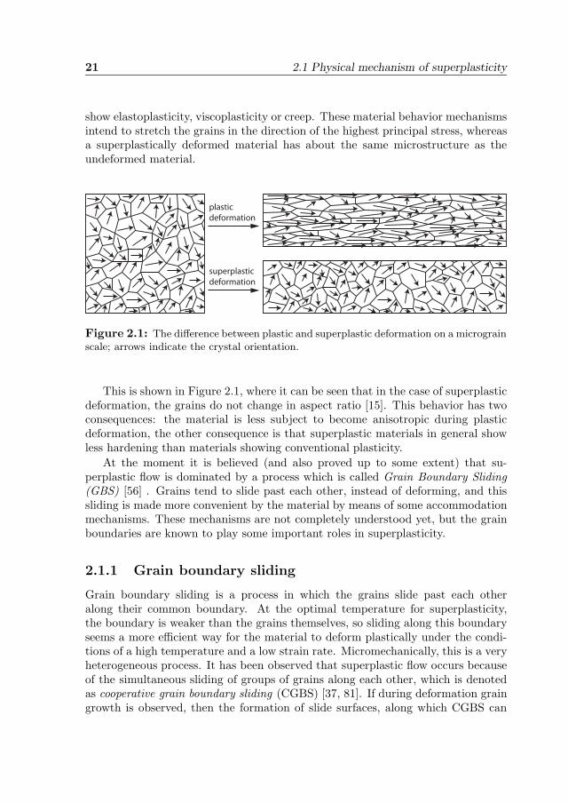
Figure 2.1: The difference between plastic and superplastic deformation on a micrograinscale; arrows indicate the crystal orientation.
This is shown in Figure 2.1, where it can be seen that in the case of superplasticdeformation, the grains do not change in aspect ratio [15]. This behavior has twoconsequences: the material is less subject to become anisotropic during plasticdeformation, the other consequence is that superplastic materials in general showless hardening than materials showing conventional plasticity.
At the moment it is believed (and also proved up to some extent) that su-perplastic flow is dominated by a process which is called Grain Boundary Sliding(GBS) [56] . Grains tend to slide past each other, instead of deforming, and thissliding is made more convenient by the material by means of some accommodationmechanisms. These mechanisms are not completely understood yet, but the grainboundaries are known to play some important roles in superplasticity.
2.1.1 Grain boundary sliding
Grain boundary sliding is a process in which the grains slide past each otheralong their common boundary. At the optimal temperature for superplasticity,the boundary is weaker than the grains themselves, so sliding along this boundaryseems a more efficient way for the material to deform plastically under the condi-tions of a high temperature and a low strain rate. Micromechanically, this is a veryheterogeneous process. It has been observed that superplastic flow occurs becauseof the simultaneous sliding of groups of grains along each other, which is denotedas cooperative grain boundary sliding (CGBS) [37, 81]. If during deformation graingrowth is observed, then the formation of slide surfaces, along which CGBS can
2 Superplasticity 22
act, is restrained, and the superplastic flow will stop. This means that grain growthhas to be prevented as much as possible in order to achieve superplastic behavior.
2.1.2 Accommodation mechanisms
If GBS were the only mechanism to occur in superplastic flow, then either thegrains would have an ideal shape, such as a square, or huge cavities would occur inthe material just before sliding takes place. Neither is the case. This means that inbetween the two grain boundary sliding steps another mechanism is responsible forthis happening; it is called an accommodation mechanism. Two mechanisms will bediscussed here, Diffusion Creep and Intragranular Slip. The mechanisms describedare still under discussion, and it is also believed that grain boundary diffusion canbe accommodated by partial melting in the boundary zone because of the elevatedtemperature. The effect of all accommodation mechanisms stays the same: takingcare of a coherent shape between the sliding grain boundaries, without introducinglarge cavities. The accommodation mechanism builds up until a certain thresholdstress. If this stress is reached, then (cooperative) grain boundary sliding will takeplace in a fraction of the time of the build-up period.
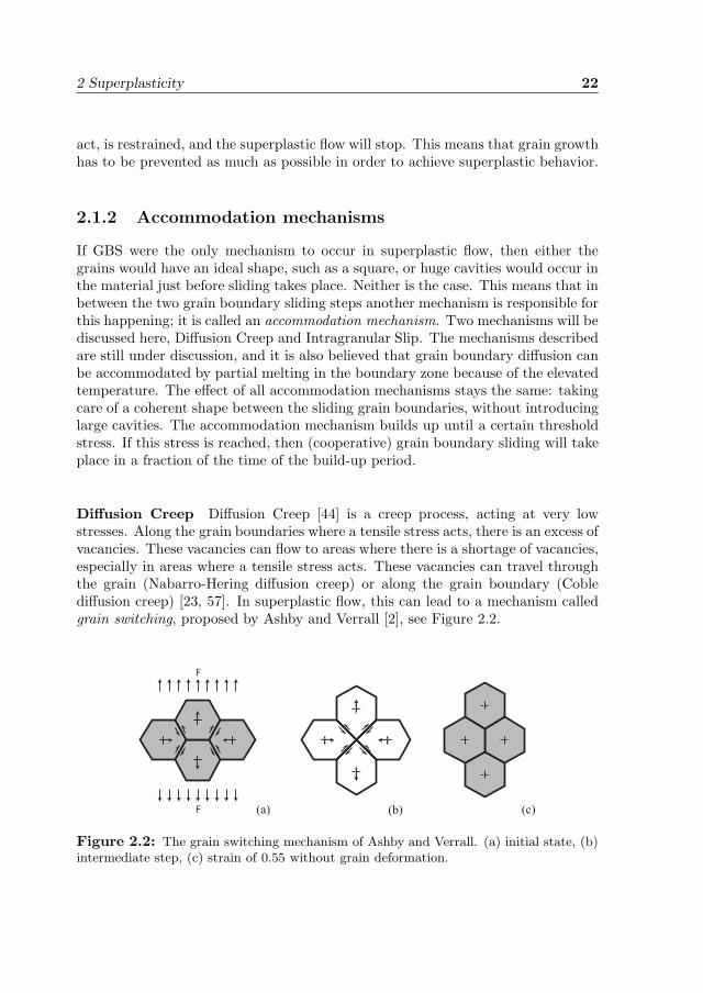
Diffusion Creep Diffusion Creep [44] is a creep process, acting at very lowstresses. Along the grain boundaries where a tensile stress acts, there is an excess ofvacancies. These vacancies can flow to areas where there is a shortage of vacancies,especially in areas where a tensile stress acts. These vacancies can travel throughthe grain (Nabarro-Hering diffusion creep) or along the grain boundary (Coblediffusion creep) [23, 57]. In superplastic flow, this can lead to a mechanism calledgrain switching, proposed by Ashby and Verrall [2], see Figure 2.2.
F
F (a) (c)(b)
Figure 2.2: The grain switching mechanism of Ashby and Verrall. (a) initial state, (b)intermediate step, (c) strain of 0.55 without grain deformation.
23 2.1 Physical mechanism of superplasticity
Intragranular Slip If a slip plane arises inside a grain, then this is called in-tragranular slip. An extra boundary can grow inside this grain due to a collectivemovement of dislocations, which can assist in the mechanism of cooperative grainboundary sliding. Such a dislocation line inside a grain will then be collinear withthe favorable sliding path. Intragranular slip is not seen in every superplastic ma-terial, this is especially seen in materials based on Al-Mg.
2.1.3 Grain growth
Since at a high enough temperature the grain boundaries in a superplastic mate-rial are weaker than the material in the grains itself, the superplastic propertiesof a material are very dependent on the grain size. There is a strong relationshipbetween the grain size and the strain rate sensitivity parameter m [3]. This param-eter determines the superplastic flow behavior, as shall be shown in Section 2.3.Because every grain boundary is an imperfection, the free energy of the materialis higher at these places. Therefore there is a tendency to grain growth to reducethis free energy. This process is temperature dependent and can be expressed as:
dg − dg0 = Bt exp(−Q/RT ) (2.1)
in which d and d0 are the current and initial grain size, B is a constant, Q isthe activation energy, R is the universal gas constant, T is the temperature andt is the time. For normal grain growth, (also called static grain growth) wherethe strain rate is zero, g is equal to 2. This is a diffusion controlled process,hence dependent on the temperature. Grain growth must be prevented as muchas possible, because the fracture strain decreases as the grain size increases. Thisreduction of free energy can also be achieved by adding mechanical energy insteadof thermal energy, which means that deforming the material also leads to graingrowth, which is called dynamic grain growth.
Superplastic alloys have generally very good resistance to both types of graingrowth, which is a result of the constituents (alloying elements). Both types ofgrain growth work independently from each other, which is, for instance, clearlyvisible from the grain size evolution law, as described in [50]:
d = Mσsurfd−r0 + αεpd−r1 (2.2)
in which r0, r1 and α are constants, M is the grain boundary mobility which istemperature dependent and σsurf is the grain boundary energy density.
Static and dynamic grain growth can conflict with each other and it is desirablethat grain growth in general must be avoided as much as possible. Dynamic graingrowth is low if the strain rate is low, but this means that the exposure time toan elevated temperature will be higher, and hence will lead to higher static graingrowth. Higher strain rates will lead to a higher dynamic grain growth, but to lowerstatic grain growth. Generally, a superplastic material has an optimum strain rateat which the superplastic properties are optimal.
2 Superplasticity 24
2.1.4 Cavity formation
If the grains were able to just slide past each other as infinitely rigid particles,then very quickly internal voids would occur, also called cavities. In the first stageof superplastic behavior, cavities do not arise, and they are normally seen duringthe last stage of superplastic flow. The cavitation process consists of three stages,which can occur simultaneously.
• cavity nucleation: this takes place at irregularities, where for instancethe accommodation mechanism cannot completely compensate for the non-coherence of the shape of adjacent grains. Most irregularities are at placeswhere the grain boundary switches orientation (at triple junctions), or atplaces where second-phase particles are present.
• cavity growth: with increasing strain, cavities can become larger. They act aslarge vacancies to where minor vacancies in the structure can diffuse, calledstress directed vacancy diffusion. Cavity growth is the cause of unstableplastic flow. An equation to describe the cavity volume fraction as a resultfrom cavity growth is found in [5]
ξ =32
(m + 1m
)sinh[2(2 − m
2 + m
)(ks
3− p
σe
)](2.3)
where m is the strain rate sensitivity, ks is a stress concentration factor de-pending on the amount of grain boundary sliding, p is the pressure and σe isthe equivalent stress.
• cavity coalescence: the internal voids start to interlink with each other tocreate a crack in the material. According to [45], the coalescence conditioncan be written as
σm
σf
1(1 − χ2)
=23
[α
(1 − χ
χW
)2
+ 1.24√
1χ
](2.4)
where σm is the matrix stress (the stress in the material around the cavities),σf is the macroscopic flow stress, χ is the relative void spacing (void meandiameter over mean void distance), W is the void aspect ratio, and α is aparameter which is 0.1 if there is no hardening present (which can be assumedat the point of void coalescence).
As said earlier, cavity forming only arises during the last stage of superplasticforming, and is an indication of fracture initiation, and therefore can lead to unre-coverable damage to the material. In an earlier stage the material starts leaking,which is more relevant in this research project. It is interesting to see that, incontrast to plasticity, cavities in superplastically formed materials are much more
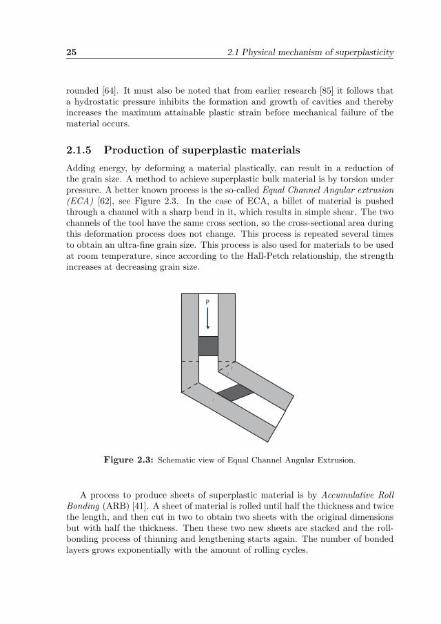
25 2.1 Physical mechanism of superplasticity
rounded [64]. It must also be noted that from earlier research [85] it follows thata hydrostatic pressure inhibits the formation and growth of cavities and therebyincreases the maximum attainable plastic strain before mechanical failure of thematerial occurs.
2.1.5 Production of superplastic materials
Adding energy, by deforming a material plastically, can result in a reduction ofthe grain size. A method to achieve superplastic bulk material is by torsion underpressure. A better known process is the so-called Equal Channel Angular extrusion(ECA) [62], see Figure 2.3. In the case of ECA, a billet of material is pushedthrough a channel with a sharp bend in it, which results in simple shear. The twochannels of the tool have the same cross section, so the cross-sectional area duringthis deformation process does not change. This process is repeated several timesto obtain an ultra-fine grain size. This process is also used for materials to be usedat room temperature, since according to the Hall-Petch relationship, the strengthincreases at decreasing grain size.
P
Figure 2.3: Schematic view of Equal Channel Angular Extrusion.
A process to produce sheets of superplastic material is by Accumulative RollBonding (ARB) [41]. A sheet of material is rolled until half the thickness and twicethe length, and then cut in two to obtain two sheets with the original dimensionsbut with half the thickness. Then these two new sheets are stacked and the roll-bonding process of thinning and lengthening starts again. The number of bondedlayers grows exponentially with the amount of rolling cycles.

2 Superplasticity 26
2.2 Superplastic materials in industry
This section elaborates on the most common materials which can be used in super-plastic deformation processes. These materials are mostly aluminum or titanium-based alloys, but some stainless steel or more exotic materials can show superplasticbehavior too. Superplastic materials contain generally dedicated alloying elements(second-phase particles), commonly functioning as a grain growth inhibitor. Thischapter focuses exclusively on the superplastic behavior of metals, this means thatpolymers and ceramic materials are excluded from the summarized materials list.Other metal alloys include, for instance, the 2205 series stainless steel, the copper-based alloy Coronze CDA-638 and the nickel-based alloy Inconel 718. Comparedto aluminum and titanium, these materials have a much higher density. This iswhy these materials are not used very often in structural applications, unless sometypical properties are desired.
2.2.1 Aluminum-based materials
Most materials which are used in superplastic forming processes, are aluminum-based materials. These materials belong to the category of pseudo-single phasematerials, with relatively small amounts of second-phase elements. They have ahigh resistance to static grain growth. Their superplastic behavior is the reasonwhy these materials are categorized under names as Supral and Formall. Typ-ical superplastic forming temperatures are about 500 to 550 oC. The density ofaluminum is about 2700 kg/m3.
Supral 100 and 150 These are the commercial names for Aluminum Alloy2004SPF which is a medium-strength alloy with mechanical properties similar toAA6061 and AA2219 and is used in lightly loaded or nonstructural applications, e.g.in the aerospace industry. It is manufactured by Superform USA, Inc. AA2004-SPF is alloyed with 6% Cu and small amounts of Mg and Zr. It can reach a nominalplastic strain before fracture of more than 200% [66].
Formall 545 and 700 Formall is the commercial name for superplastic alu-minum alloys manufactured by Alusuisse Swiss aluminum and comes in two alloytypes, AA5083-SPF and AA7475-SPF, respectively. In AA5083, the main alloyingelement besides aluminum present in this alloy is magnesium; in AA7475 zinc andcopper are the main alloying elements [17]. For these materials, some superplasticmaterial data was found in the literature. AA5083-SPF has a strain rate sensitivityparameter of 0.60 at a flow stress of 3 MPa, whereas AA7475-SPF has a strain ratesensitivity parameter of 0.70 at a flow stress of 3 MPa at the superplastic temper-ature. Applications are, for instance, car body panels in the automotive industry.The maximum nominal plastic strain before fracture is about 400 % [83].

27 2.2 Superplastic materials in industry
2.2.2 Titanium-based materials
Titanium has a much higher melting point in comparison with aluminum, the su-perplastic processing temperature of titanium-based alloys is about 900 oC. Belowthis temperature, pure titanium consists of a hexagonal close-packed structure,called the α-phase. Above this temperature, the structure is body-centered cubic,which is called the β-phase. The α-phase is particularly useful in cryogenic ap-plications, where the material has its best strength properties, whereas at roomtemperature the strength is low. The β-phase has a much higher strength at roomtemperature, but this phase can only be contained at room temperature if the ma-terial is solution-treated with e.g. vanadium. Superplastic behavior of titaniumalloys can only be observed in a mix of the two phases, so stabilizers should beadded to ensure that these two phases keep existing in the alloy. Aluminum, whichcan be added up to 8%, is an α-stabilizer, whereas molybdenum and vanadium arethe best known β-stabilizers. The density of titanium is about 4300 kg/m3.
Ti-6Al-4V alloy This is the most used superplastic titanium alloy, especiallyfor the manufacturing of structural aircraft parts. It has a superior strength-to-weight ratio and corrosion resistance at high temperatures. Its optimum formingtemperature with respect to superplasticity is 800 oC, but the range of temperaturesin which superplastic behavior is active is quite broad (between 700 and 950 oC)[70]. At room temperature, the maximum elongation is about 20%, but this valueincreases quickly starting at a temperature of about 500 oC to a value of about300% at the optimal superplastic temperature [36]. Above 800 oC, the materialsuffers from dynamic grain growth, which then will be more dominant with respectto dynamic recrystallization.
Ti 14-25% Al 10-20% Nb 3% V 2% Mo This special alloy is also called SuperAlpha 2 and is actually an alloy of titanium aluminide. The aluminide shows verybrittle behavior, the addition of niobium makes the material ductile. This alloy hasan excellent oxidation resistance at high temperatures, which makes it a suitablematerial for use in jet engines and supersonic aircraft. At room temperature, thismaterial shows very brittle behavior. This material is, in contrast to the pseudo-single phase materials, a mixture of grains of the matrix phase and grains of thealloying phase, a so-called microduplex superplastic alloy. The optimal superplastictemperature is about 960 oC [65], showing an elongation of more than 1000 %.
2.2.3 ALNOVI-1
ALNOVI-1 is a relatively new material also based on AA5083, manufactured byFurukawa Sky aluminum, Japan [25, 78]. It is designated a superplastic material,although it does not reach the extremely high plastic strains which can be reachedby other superplastic materials. A grain growth inhibitor is added (0.8% Mn). At
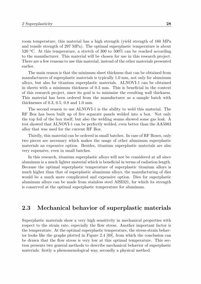
2 Superplasticity 28
room temperature, this material has a high strength (yield strength of 160 MPaand tensile strength of 297 MPa). The optimal superplastic temperature is about520 oC. At this temperature, a stretch of 300 to 500% can be reached accordingto the manufacturer. This material will be chosen for use in this research project.There are a few reasons to use this material, instead of the other materials presentedearlier.
The main reason is that the minimum sheet thickness that can be obtained frommanufacturers of superplastic materials is typically 1.0 mm, not only for aluminumalloys, but also for titanium superplastic materials. ALNOVI-1 can be obtainedin sheets with a minimum thickness of 0.3 mm. This is beneficial in the contextof this research project, since its goal is to minimize the resulting wall thickness.This material has been ordered from the manufacturer as a sample batch withthicknesses of 0.3, 0.5, 0.8 and 1.0 mm.
The second reason to use ALNOVI-1 is the ability to weld this material. TheRF Box has been built up of five separate panels welded into a box. Not onlythe top foil of the box itself, but also the welding seams showed some gas leak. Atest showed that ALNOVI-1 can be perfectly welded, even better than the AA5083alloy that was used for the current RF Box.
Thirdly, this material can be ordered in small batches. In case of RF Boxes, onlytwo pieces are necessary which makes the usage of other aluminum superplasticmaterials an expensive option. Besides, titanium superplastic materials are alsovery expensive, even in small batches.
In this research, titanium superplastic alloys will not be considered at all sincealuminum is a much lighter material which is beneficial in terms of radiation length.Because the optimal superplastic temperature of superplastic titanium alloys ismuch higher than that of superplastic aluminum alloys, the manufacturing of dieswould be a much more complicated and expensive option. Dies for superplasticaluminum alloys can be made from stainless steel AISI321, for which its strengthis conserved at the optimal superplastic temperature for aluminum.
2.3 Mechanical behavior of superplastic materials
Superplastic materials show a very high sensitivity in mechanical properties withrespect to the strain rate, especially the flow stress. Another important factor isthe temperature. At the optimal superplastic temperature, the stress-strain behav-ior looks like the graphs plotted in Figure 2.4 [69], from which the conclusion canbe drawn that the flow stress is very low at this optimal temperature. This sec-tion presents two general methods to describe mechanical behavior of superplasticmaterials: firstly a phenomenological way, secondly a physical method.
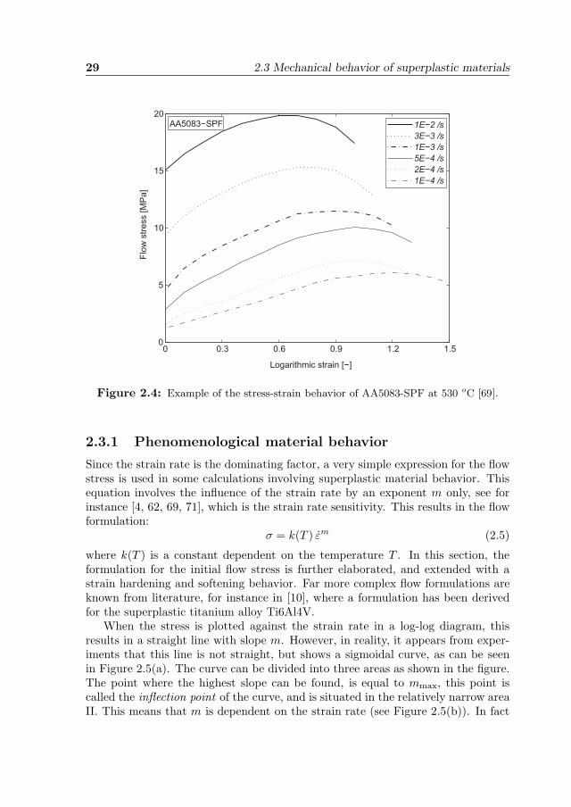
29 2.3 Mechanical behavior of superplastic materials
0 0.3 0.6 0.9 1.2 1.50
5
10
15
20
Logarithmic strain [−]
Flo
w s
tress [M
Pa]
1E−2 /s3E−3 /s1E−3 /s5E−4 /s2E−4 /s1E−4 /s
AA5083−SPF
Figure 2.4: Example of the stress-strain behavior of AA5083-SPF at 530 oC [69].
2.3.1 Phenomenological material behavior
Since the strain rate is the dominating factor, a very simple expression for the flowstress is used in some calculations involving superplastic material behavior. Thisequation involves the influence of the strain rate by an exponent m only, see forinstance [4, 62, 69, 71], which is the strain rate sensitivity. This results in the flowformulation:
σ = k(T ) εm (2.5)
where k(T ) is a constant dependent on the temperature T . In this section, theformulation for the initial flow stress is further elaborated, and extended with astrain hardening and softening behavior. Far more complex flow formulations areknown from literature, for instance in [10], where a formulation has been derivedfor the superplastic titanium alloy Ti6Al4V.
When the stress is plotted against the strain rate in a log-log diagram, thisresults in a straight line with slope m. However, in reality, it appears from exper-iments that this line is not straight, but shows a sigmoidal curve, as can be seenin Figure 2.5(a). The curve can be divided into three areas as shown in the figure.The point where the highest slope can be found, is equal to mmax, this point iscalled the inflection point of the curve, and is situated in the relatively narrow areaII. This means that m is dependent on the strain rate (see Figure 2.5(b)). In fact
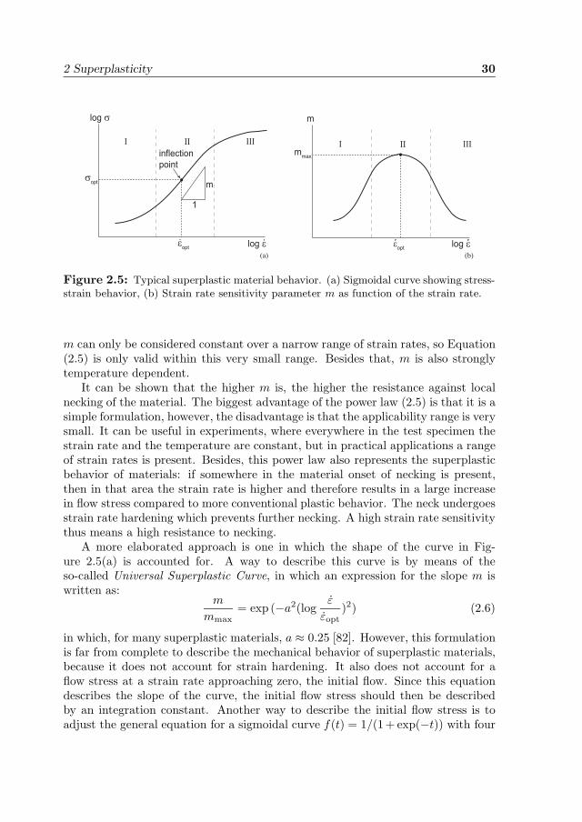
2 Superplasticity 30
m
1
inflection
point
I IIIII
log ε
log σ
εopt
σopt
I IIIII
log ε
m
εopt
mmax
(a) (b)
Figure 2.5: Typical superplastic material behavior. (a) Sigmoidal curve showing stress-strain behavior, (b) Strain rate sensitivity parameter m as function of the strain rate.
m can only be considered constant over a narrow range of strain rates, so Equation(2.5) is only valid within this very small range. Besides that, m is also stronglytemperature dependent.
It can be shown that the higher m is, the higher the resistance against localnecking of the material. The biggest advantage of the power law (2.5) is that it is asimple formulation, however, the disadvantage is that the applicability range is verysmall. It can be useful in experiments, where everywhere in the test specimen thestrain rate and the temperature are constant, but in practical applications a rangeof strain rates is present. Besides, this power law also represents the superplasticbehavior of materials: if somewhere in the material onset of necking is present,then in that area the strain rate is higher and therefore results in a large increasein flow stress compared to more conventional plastic behavior. The neck undergoesstrain rate hardening which prevents further necking. A high strain rate sensitivitythus means a high resistance to necking.
A more elaborated approach is one in which the shape of the curve in Fig-ure 2.5(a) is accounted for. A way to describe this curve is by means of theso-called Universal Superplastic Curve, in which an expression for the slope m iswritten as:
m
mmax= exp (−a2(log
ε
εopt)2) (2.6)
in which, for many superplastic materials, a ≈ 0.25 [82]. However, this formulationis far from complete to describe the mechanical behavior of superplastic materials,because it does not account for strain hardening. It also does not account for aflow stress at a strain rate approaching zero, the initial flow. Since this equationdescribes the slope of the curve, the initial flow stress should then be describedby an integration constant. Another way to describe the initial flow stress is toadjust the general equation for a sigmoidal curve f(t) = 1/(1+ exp(−t)) with four
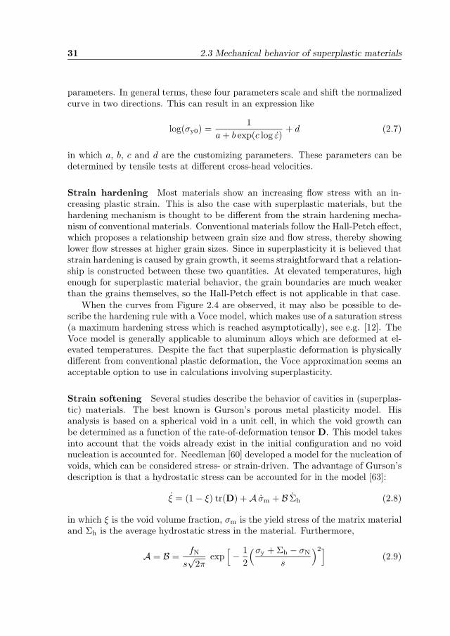
31 2.3 Mechanical behavior of superplastic materials
parameters. In general terms, these four parameters scale and shift the normalizedcurve in two directions. This can result in an expression like
log(σy0) =1
a + b exp(c log ε)+ d (2.7)
in which a, b, c and d are the customizing parameters. These parameters can bedetermined by tensile tests at different cross-head velocities.
Strain hardening Most materials show an increasing flow stress with an in-creasing plastic strain. This is also the case with superplastic materials, but thehardening mechanism is thought to be different from the strain hardening mecha-nism of conventional materials. Conventional materials follow the Hall-Petch effect,which proposes a relationship between grain size and flow stress, thereby showinglower flow stresses at higher grain sizes. Since in superplasticity it is believed thatstrain hardening is caused by grain growth, it seems straightforward that a relation-ship is constructed between these two quantities. At elevated temperatures, highenough for superplastic material behavior, the grain boundaries are much weakerthan the grains themselves, so the Hall-Petch effect is not applicable in that case.
When the curves from Figure 2.4 are observed, it may also be possible to de-scribe the hardening rule with a Voce model, which makes use of a saturation stress(a maximum hardening stress which is reached asymptotically), see e.g. [12]. TheVoce model is generally applicable to aluminum alloys which are deformed at el-evated temperatures. Despite the fact that superplastic deformation is physicallydifferent from conventional plastic deformation, the Voce approximation seems anacceptable option to use in calculations involving superplasticity.
Strain softening Several studies describe the behavior of cavities in (superplas-tic) materials. The best known is Gurson’s porous metal plasticity model. Hisanalysis is based on a spherical void in a unit cell, in which the void growth canbe determined as a function of the rate-of-deformation tensor D. This model takesinto account that the voids already exist in the initial configuration and no voidnucleation is accounted for. Needleman [60] developed a model for the nucleation ofvoids, which can be considered stress- or strain-driven. The advantage of Gurson’sdescription is that a hydrostatic stress can be accounted for in the model [63]:
ξ = (1 − ξ) tr(D) + A σm + B Σh (2.8)
in which ξ is the void volume fraction, σm is the yield stress of the matrix materialand Σh is the average hydrostatic stress in the material. Furthermore,
A = B =fN
s√
2πexp[− 1
2
(σy + Σh − σN
s
)2](2.9)
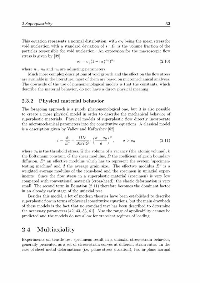
2 Superplasticity 32
This equation represents a normal distribution, with σN being the mean stress forvoid nucleation with a standard deviation of s. fN is the volume fraction of theparticles responsible for void nucleation. An expression for the macroscopic flowstress is given by [39]
σf = σy(1 − n1ξn2)n3 (2.10)
where n1, n2 and n3 are adjusting parameters.Much more complex descriptions of void growth and the effect on the flow stress
are available in the literature, most of them are based on micromechanical analyses.The downside of the use of phenomenological models is that the constants, whichdescribe the material behavior, do not have a direct physical meaning.
2.3.2 Physical material behavior
The foregoing approach is a purely phenomenological one, but it is also possibleto create a more physical model in order to describe the mechanical behavior ofsuperplastic materials. Physical models of superplastic flow directly incorporatethe micromechanical parameters into the constitutive equations. A classical modelis a description given by Valiev and Kaibyshev [62]:
ε =σ
E∗ +ΩD
16kTG·(σ − σ0
d
)2
, σ > σ0 (2.11)
where σ0 is the threshold stress, Ω the volume of a vacancy (the atomic volume), kthe Boltzmann constant, G the shear modulus, D the coefficient of grain boundarydiffusion, E∗ an effective modulus which has to represent the system ’specimen-testing machine’ and d the average grain size. The effective modulus E∗ is aweighted average modulus of the cross-head and the specimen in uniaxial exper-iments. Since the flow stress in a superplastic material (specimen) is very lowcompared with conventional materials (cross-head), the elastic deformation is verysmall. The second term in Equation (2.11) therefore becomes the dominant factorin an already early stage of the uniaxial test.
Besides this model, a lot of modern theories have been established to describesuperplastic flow in terms of physical constitutive equations, but the main drawbackof these models is the fact that no standard test has been described to determinethe necessary parameters [42, 43, 53, 61]. Also the range of applicability cannot bepredicted and the models do not allow for transient regimes of loading.
2.4 Multiaxiality
Experiments on tensile test specimens result in a uniaxial stress-strain behavior,generally presented as a set of stress-strain curves at different strain rates. In thecase of sheet metal deformations (i.e. plane stress situation), two in-plane normal
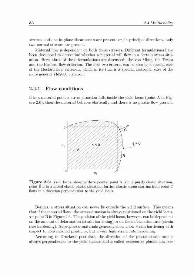
33 2.4 Multiaxiality
stresses and one in-plane shear stress are present; or, in principal directions, onlytwo normal stresses are present.
Material flow is dependent on both these stresses. Different formulations havebeen developed to determine whether a material will flow in a certain stress situ-ation. Here, three of these formulations are discussed: the von Mises, the Trescaand the Hosford flow criterion. The first two criteria can be seen as a special caseof the Hosford flow criterion, which in its turn is a special, isotropic, case of themore general Yld2000 criterion.
2.4.1 Flow conditions
If in a material point a stress situation falls inside the yield locus (point A in Fig-ure 2.6), then the material behaves elastically and there is no plastic flow present.
σ1
σ2
0
A
B
C
φ φ = 0< 0
Figure 2.6: Yield locus, showing three points: point A is in a purely elastic situation,point B is in a mixed elastic-plastic situation, further plastic strain starting from point Cflows in a direction perpendicular to the yield locus.
Besides, a stress situation can never lie outside the yield surface. This meansthat if the material flows, the stress situation is always positioned on the yield locus,see point B in Figure 2.6. The position of the yield locus, however, can be dependenton the amount of deformation (strain hardening) or on the deformation rate (strainrate hardening). Superplastic materials generally show a low strain hardening withrespect to conventional plasticity, but a very high strain rate hardening.
According to Drucker’s postulate, the direction of the plastic strain rate isalways perpendicular to the yield surface and is called associative plastic flow; see
2 Superplasticity 34
point C in Figure 2.6
Dp = λ∂φ
∂σ(2.12)
in which λ is the plastic multiplier. Two assumptions are generally made in plasticflow theory which may not be directly applicable to superplastic flow:
• the position of the yield surface is independent of the hydrostatic pressure. Itis known that failure of superplastic materials is caused by cavity formationin the material and it is believed that the application of a backpressure caninhibit this effect.
• the volume of the material during plastic flow is constant. In superplasticity,the macroscopic volume increases due to cavity formation.
This means that strictly speaking the flow behavior is non-associative. Generally,the hydrostatic pressure, which is caused by application of a backpressure duringthe deformation process, does not change. This makes the use of a non-associativeflow model unnecessary if the hydrostatic pressure only influences the void volumefraction and does not change the relationship between the void volume fraction andthe softening stress.
2.4.2 Yield criteria
A yield criterion is always formulated in such a way that a value, represented as φ,is smaller than zero if the stress situation falls inside the yield surface and zero incase it falls on the yield surface. The Kuhn-Tucker relations have to be satisfied:
λ ≥ 0φ ≤ 0
λφ = 0
(2.13)
In metal plasticity calculations, the von Mises yield criterion is mostly used forisotropic material behavior. Because superplastic materials are known to behavein an isotropic way, three yield criteria will be discussed here which can be used forthis purpose: von Mises as the most common criterion, the Tresca criterion as alimit situation, and the Hosford criterion as a generalization of both these criteria.These three criteria can all be considered as derived from the more general Yld2000flow criterion [9, 86], an orthotropic yield function applicable to sheet material(plane stress).
Von Mises yield criterion If projected onto the π plane, which is the crosssection of the yield surface perpendicular to the line σ1 = σ2 = σ3, the yield locusis a circle. The von Mises yield criterion is based on the assumption that a material
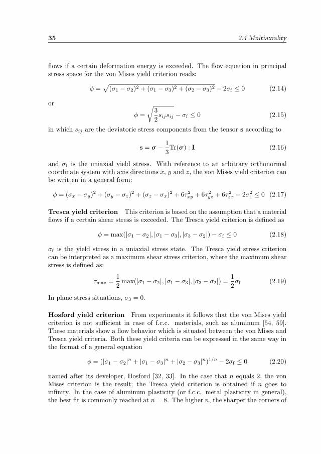
35 2.4 Multiaxiality
flows if a certain deformation energy is exceeded. The flow equation in principalstress space for the von Mises yield criterion reads:
φ =√
(σ1 − σ2)2 + (σ1 − σ3)2 + (σ2 − σ3)2 − 2σf ≤ 0 (2.14)
or
φ =
√32sijsij − σf ≤ 0 (2.15)
in which sij are the deviatoric stress components from the tensor s according to
s = σ − 13Tr(σ) : I (2.16)
and σf is the uniaxial yield stress. With reference to an arbitrary orthonormalcoordinate system with axis directions x, y and z, the von Mises yield criterion canbe written in a general form:
φ = (σx − σy)2 + (σy − σz)2 + (σz − σx)2 + 6τ2xy + 6τ2
yz + 6τ2zx − 2σ2
f ≤ 0 (2.17)
Tresca yield criterion This criterion is based on the assumption that a materialflows if a certain shear stress is exceeded. The Tresca yield criterion is defined as
φ = max(|σ1 − σ2|, |σ1 − σ3|, |σ3 − σ2|) − σf ≤ 0 (2.18)
σf is the yield stress in a uniaxial stress state. The Tresca yield stress criterioncan be interpreted as a maximum shear stress criterion, where the maximum shearstress is defined as:
τmax =12
max(|σ1 − σ2|, |σ1 − σ3|, |σ3 − σ2|) =12σf (2.19)
In plane stress situations, σ3 = 0.
Hosford yield criterion From experiments it follows that the von Mises yieldcriterion is not sufficient in case of f.c.c. materials, such as aluminum [54, 59].These materials show a flow behavior which is situated between the von Mises andTresca yield criteria. Both these yield criteria can be expressed in the same way inthe format of a general equation
φ = (|σ1 − σ2|n + |σ1 − σ3|n + |σ2 − σ3|n)1/n − 2σf ≤ 0 (2.20)
named after its developer, Hosford [32, 33]. In the case that n equals 2, the vonMises criterion is the result; the Tresca yield criterion is obtained if n goes toinfinity. In the case of aluminum plasticity (or f.c.c. metal plasticity in general),the best fit is commonly reached at n = 8. The higher n, the sharper the corners of
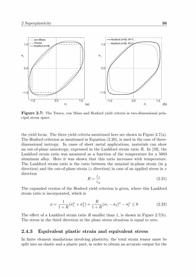
2 Superplasticity 36
−1.0 0.0 1.0
−1.0
0.0
1.0
von MisesTrescaHosford (n=8)
σ1
σ2
−1.0 0.0 1.0
−1.0
0.0
1.0
Hosford (n=8): R=1
σ1
σ2
Hosford (n=8): R<1
(a) (b)
Figure 2.7: The Tresca, von Mises and Hosford yield criteria in two-dimensional prin-cipal stress space.
the yield locus. The three yield criteria mentioned here are shown in Figure 2.7(a).The Hosford criterion as mentioned in Equation (2.20), is used in the case of three-dimensional isotropy. In cases of sheet metal applications, materials can showan out-of-plane anisotropy, expressed in the Lankford strain ratio R. In [59], theLankford strain ratio was measured as a function of the temperature for a 5083aluminum alloy. Here it was shown that this ratio increases with temperature.The Lankford strain ratio is the ratio between the uniaxial in-plane strain (in ydirection) and the out-of-plane strain (z direction) in case of an applied stress in xdirection
R =εz
εy(2.21)
The expanded version of the Hosford yield criterion is given, where this Lankfordstrain ratio is incorporated, which is
φ =1
1 + R(σn
1 + σn2 ) +
R
1 + R(σ1 − σ2)n − σn
f ≤ 0 (2.22)
The effect of a Lankford strain ratio R smaller than 1, is shown in Figure 2.7(b).The stress in the third direction in the plane stress situation is equal to zero.
2.4.3 Equivalent plastic strain and equivalent stress
In finite element simulations involving plasticity, the total strain tensor must besplit into an elastic and a plastic part, in order to obtain an accurate output for the
37 2.4 Multiaxiality
stress tensor. The stresses and plastic strains can be calculated using an iterativescheme (e.g. a Newton iteration scheme). In this iterative scheme, it is much moreconvenient to use single scalar values for the plastic strain and stress, therefore anequivalent value for the strain and stress tensor must be defined. From uniaxialtensile experiments, a plastic strain state can be determined relatively easily fromthe elongation. A stretch λ can be translated into a strain ε by using one of severaldifferent formulations. The most used is the logarithmic or true strain, which isdefined as
εl = ln λ (2.23)
In a uniaxial stress situation, the strains in the perpendicular directions are non-zero, but can be easily determined because the stresses in these directions arezero. In case of plasticity, these strains are such that the material volume does notchange (which is not necessarily the case in superplasticity, if the macro-volume isconsidered, see Section 2.4.1).
In a 2- or 3-dimensional stress situation, it is convenient to compare the strainsand stresses in the material with the strains and stresses as found in a uniaxialsituation. Therefore, an equivalent plastic strain can be defined, which is
εp =∫ t
t0
εpdt (2.24)
in which εp is the equivalent plastic strain rate and is defined in terms of theplastic part of the rate-of-deformation tensor Dp, which is in the case of von Misesplasticity
εp =
√23Dp : Dp (2.25)
The von Mises equivalent stress shows a comparable equation
σeqy =
√32s : s (2.26)
where s represents the deviatoric stress tensor. The relationship between equivalentstress and equivalent plastic strain in a material is the same as its uniaxial stress-strain relationship.
These formulations of equivalent strain and stress become different if the Hos-ford yield criterion is used, but the idea is the same: constructing a useful scalarvalue which can be compared with a uniaxial situation. Equations (2.20) and (2.22)give the equivalent stress in the case of Hosford flow. The equivalent plastic straincan be determined by generalizing an alternative formulation
σeqy εp = σ : Dp (2.27)
Represented as a one-dimensional stress vector and a two-dimensional rate-of-deformation tensor. Unfortunately, where the equivalent stress in case of von Mises
2 Superplasticity 38
flow can be easily expressed in terms of the deviatoric stress tensor, in the case ofthe Hosford yield criterion this is not possible. The double dot product betweentwo 2-dimensional (stress) tensors gives a scalar value, just as the equivalent stress.In the case of the Hosford yield criterion, higher (n) double dot multiplications arenot possible, so a scalar value cannot be the output. The equivalent stress musttherefore be expressed in the stress tensor elements only, rather than by the stresstensor as a whole.
2.5 Hydrostatic pressure dependence
Since the flow stresses of superplastic materials are very low (at the optimal super-plastic temperature and strain rate this is in the order of a few MPa), it is possibleto influence the flow behavior with a hydrostatic pressure. This pressure then canact as a cavity growth inhibitor [20]. This means that the material can reach ahigher plastic strain before failure. In [78] it is shown that in free bulging tests, themaximum bulge height reaches higher values if a backpressure of 14 bar is appliedduring the forming stage.
In essence, this would mean that a non-associative flow model has to be usedwhen considering pressure-dependent material behavior. In pressure-dependentmaterial models, such as the Mohr-Coulomb criterion, the hydrostatic pressure isan extra variable in the description of flow. However, when considering superplasticsheet metal forming, the applied backpressure is not a variable, but it is constantduring the whole deformation process. Therefore, it is not necessary to implementthe effect of an applied backpressure into the biaxial flow formulation, it is sufficientto describe the application of such a pressure in the uniaxial stress-strain descriptiononly.
Since the formulation of cavities is postponed to higher plastic strains at higherbackpressure, the material has a higher strength at the same plastic strain. If thevoid volume fraction is low, this is a minor effect, but this effect will increase ifthe void volume fraction becomes higher, so at higher plastic strains. The effectof an applied backpressure to a superplastic material on the uniaxial flow stress isqualitatively depicted in Figure 2.8.
2.6 Computational (super-)plasticity
Consider a material point in a structure where a prescribed strain increment isapplied. If it is known that the material will behave in a purely elastic manner,it is easy to find the accompanying stress increment. The stress situation at thismaterial point can be derived in this case from the elastic properties, i.e. Young’sModulus E and Poisson’s ratio ν. The relationship between stress and strain is de-scribed by a fourth-order elasticity tensor 4C if the stress and strain are represented
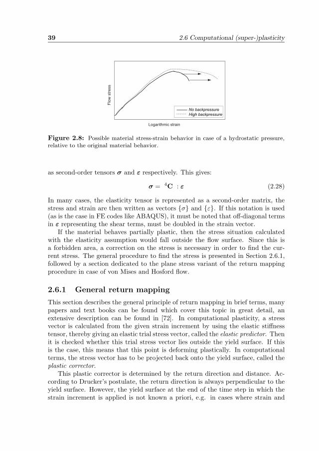
39 2.6 Computational (super-)plasticity
Logarithmic strain
Flo
w s
tre
ss
No backpressureHigh backpressure
Figure 2.8: Possible material stress-strain behavior in case of a hydrostatic pressure,relative to the original material behavior.
as second-order tensors σ and ε respectively. This gives:
σ = 4C : ε (2.28)
In many cases, the elasticity tensor is represented as a second-order matrix, thestress and strain are then written as vectors {σ} and {ε}. If this notation is used(as is the case in FE codes like ABAQUS), it must be noted that off-diagonal termsin ε representing the shear terms, must be doubled in the strain vector.
If the material behaves partially plastic, then the stress situation calculatedwith the elasticity assumption would fall outside the flow surface. Since this isa forbidden area, a correction on the stress is necessary in order to find the cur-rent stress. The general procedure to find the stress is presented in Section 2.6.1,followed by a section dedicated to the plane stress variant of the return mappingprocedure in case of von Mises and Hosford flow.
2.6.1 General return mapping
This section describes the general principle of return mapping in brief terms, manypapers and text books can be found which cover this topic in great detail, anextensive description can be found in [72]. In computational plasticity, a stressvector is calculated from the given strain increment by using the elastic stiffnesstensor, thereby giving an elastic trial stress vector, called the elastic predictor. Thenit is checked whether this trial stress vector lies outside the yield surface. If thisis the case, this means that this point is deforming plastically. In computationalterms, the stress vector has to be projected back onto the yield surface, called theplastic corrector.
This plastic corrector is determined by the return direction and distance. Ac-cording to Drucker’s postulate, the return direction is always perpendicular to theyield surface. However, the yield surface at the end of the time step in which thestrain increment is applied is not known a priori, e.g. in cases where strain and
2 Superplasticity 40
strain rate hardening are present. The return distance is expressed in the plasticmultiplier λ.A method to find the updated stress is to draw a virtual yield surface through thepoint where the elastic prediction is situated. The direction perpendicular to theyield surface, in the point of the stress situation at the beginning of the time step,is chosen to be the return direction. The return distance is determined by theplastic multiplier. The advantage of this explicit, Euler forward, return mappingalgorithm is that it is a relatively fast method. The main drawback is that thismethod is not very robust, the chosen return direction has the risk tendency to’miss’ the yield locus where it should return to. The deviation from the solutionis dependent on the strain increment. The higher this strain increment, the higherthe deviation, the calculated solution will drift away from the correct solution.
The implicit, backward Euler method looks for a solution where the returndirection is perpendicular to the yield surface at the end of the time step in whichthe strain increment is applied. This is a more complicated method to implement,but generally leads to a more accurate solution. The main advantage of the EulerBackward method is that it is unconditionally stable, whereas the Euler Forwardmethod is only conditionally stable (condition of a maximum critical time step).The return direction and distance have to be determined in an iterative process.Because of the higher stability and assumed accuracy, the Euler Backward methodwill be adapted throughout the rest of this section as the method to be implementedin the superplastic flow analyses.
2.6.2 Plane stress return mapping
In sheet metal forming computations, the in-plane dimensions are considerablylarger than the dimensions in the thickness direction. A consequence is that thestress in the thickness direction may be considered to be equal to zero, leading toa situation of plane stress. The elasticity equation (2.28) in the case of plane stressand isotropic elastic material behavior becomes
σtr =
⎧⎨⎩
σxx
σyy
σxy
⎫⎬⎭ =
E
1 − ν2
⎡⎣1 ν 0ν 1 00 0 (1 − ν)/2
⎤⎦⎧⎨⎩
εxx
εyy
γxy
⎫⎬⎭ (2.29)
where γxy is twice the engineering strain εxy, and σtr is the trial stress vector. Thestrain in thickness direction cannot be derived from the stress in that direction,since this stress is zero. Therefore an extra constraint is necessary with respectto the plastic thickness strain. This constraint states that the material volume isconserved during plastic deformation. Therefore
εpzz = −(εp
xx + εpyy) (2.30)
The plane stress problem in case of J2 (von Mises) plasticity is, for example, writ-ten out in [72]. Here, it is convenient to write the stresses in terms of the deviatoric
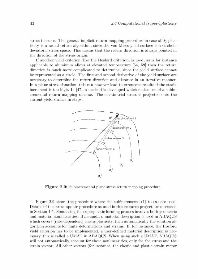
41 2.6 Computational (super-)plasticity
stress tensor s. The general implicit return mapping procedure in case of J2 plas-ticity is a radial return algorithm, since the von Mises yield surface is a circle indeviatoric stress space. This means that the return direction is always pointed inthe direction of the stress origin.
If another yield criterion, like the Hosford criterion, is used, as is for instanceapplicable to aluminum alloys at elevated temperature [54, 59] then the returndirection is much more complicated to determine, since the yield surface cannotbe represented as a circle. The first and second derivative of the yield surface arenecessary to determine the return direction and distance in an iterative manner.In a plane stress situation, this can however lead to erroneous results if the strainincrement is too high. In [47], a method is developed which makes use of a subin-cremental return mapping scheme. The elastic trial stress is projected onto thecurrent yield surface in steps.
σtrsubincrement 1
subincrement 2
subincrement 3
subincrement n
σn
f
σ1
f
σ2
f
σ3
f
Figure 2.9: Subincremental plane stress return mapping procedure.
Figure 2.9 shows the procedure where the subincrements (1) to (n) are used.Details of the stress update procedure as used in this research project are discussedin Section 4.5. Simulating the superplastic forming process involves both geometricand material nonlinearities. If a standard material description is used in ABAQUSwhich covers (rate-dependent) elasto-plasticity, then automatically the solution al-gorithm accounts for finite deformations and strains. If, for instance, the Hosfordyield criterion has to be implemented, a user-defined material description is nec-essary, this is called a UMAT in ABAQUS. When using such a UMAT, ABAQUSwill not automatically account for these nonlinearities, only for the stress and thestrain vector. All other vectors (for instance, the elastic and plastic strain vector
2 Superplasticity 42
which should be programmed as state variables) should account for these nonlin-earities within the user subroutine itself. ABAQUS provides a utility routine forthis purpose, called rotsig [75], for rotating strain-like or stress-like vectors. Thedifference between these two lie in the fact that the third term in these vectors (theshear term) must be doubled or not.
2.7 Summary and conclusions
This chapter describes the properties of superplastic materials and the phenomenonof superplasticity. Superplastic forming of the RF Foil seems an attractive alter-native for the manufacturing process which is currently used. The main reason forthis process to apply is the extremely high plastic strains which can be reached withthese materials in the forming process without failure. In the case of the RF Foil,the failure is defined by a maximum leak rate. Applying a backpressure during theforming process will increase the maximum plastic strain because void nucleationand growth is then postponed. Therefore, by increasing the backpressure duringforming, leaking is far less likely to occur in a formed sheet. Superplastic form-ing is a slow process, but this is not an issue if only a few products have to bemanufactured.
Superplastic materials come mainly as aluminum or titanium alloys. Withrespect to the material property radiation length, the use of aluminum is preferredabove titanium. The position of the element Aluminum compared with the elementTitanium in the periodic table of elements explains this preference. Some aluminumsuperplastic materials have been described, of which ALNOVI-1 is the best choice.
The mechanical behavior is discussed, where phenomenological and physicalbehavior has been distinguished. The choice has been made to use a phenomeno-logical material description. The flow stress behavior has been split into threeparts:
• the initial flow stress as a function of the equivalent plastic strain rate;
• the hardening stress, which is caused by grain growth, and is best describedby a Voce hardening law;
• the softening stress, caused by void nucleation, growth and (eventually) coa-lescence.
When considering plane stress, a more general description of the von Mises flowbehavior will be used, namely the Hosford flow criterion.
The plane stress calculations will be carried out by using an Euler Backwardreturn mapping algorithm. This scheme is unconditionally stable and yields ingeneral better results than the, easier to implement, Euler Forward return mappingscheme.
3. Material experiments
The accuracy of finite element analysis results involving (visco-)plasticity stronglydepends on the material modeling. In order to extract the desired material proper-ties, experiments are necessary to obtain uniaxial behavior expressed in stress-strainrelationships. Biaxial experiments determine the basis for biaxial flow behavior. Inthis research, the superplastic aluminum alloy ALNOVI-1 is used. This chapter isdedicated to the setup and results of the uniaxial and biaxial experiments carriedout on ALNOVI-1. Section 3.1 describes the experimental setup of the tensile testsand the specimen geometry. The raw data as obtained from these experiments arepresented as force-displacement curves. These curves are translated into uniaxialstress-strain behavior by using inverse FE modeling of the tensile tests. The stress-strain relationships are used to design the bulge experiments. Also, void growthbehavior as a function of plastic strain and strain rate is observed.
One of the most important properties to know about the material is the per-meability of the deformed material with respect to gases. Before the material failsby fracture, enough voids may have been formed, grown, or may even be inter-linked, to provide a leak channel through the thickness of the formed material.An experiment has been designed where circular sheets are freely blown into a,practically endless, cylindrical tool. Another extra input that can be accountedfor, which which was not the case in the tensile experiments, is the application of abackpressure during the test. In Chapter 2, it was mentioned that a backpressureslows down the process of cavity growth, which has a beneficial effect on the gaspermeability. Section 3.2 describes the free bulging experiments, whereas Section3.3 presents the leak measurements from these experiments.
Section 3.4 concerns the forming of the sheets into a die, in order to obtainfriction information between the sheet and the die. A die shape has been designedwhere the resulting thickness of the sheet can be measured in two points. Thethickness ratio between these two points is a measure for the friction coefficient.
3.1 Uniaxial material experiments
The purpose of the tensile experiments is to gather information about the uniaxialmechanical behavior of ALNOVI-1. Tensile tests until fracture are performed which
43
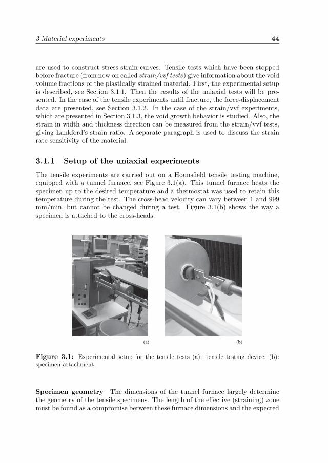
3 Material experiments 44
are used to construct stress-strain curves. Tensile tests which have been stoppedbefore fracture (from now on called strain/vvf tests) give information about the voidvolume fractions of the plastically strained material. First, the experimental setupis described, see Section 3.1.1. Then the results of the uniaxial tests will be pre-sented. In the case of the tensile experiments until fracture, the force-displacementdata are presented, see Section 3.1.2. In the case of the strain/vvf experiments,which are presented in Section 3.1.3, the void growth behavior is studied. Also, thestrain in width and thickness direction can be measured from the strain/vvf tests,giving Lankford’s strain ratio. A separate paragraph is used to discuss the strainrate sensitivity of the material.
3.1.1 Setup of the uniaxial experiments
The tensile experiments are carried out on a Hounsfield tensile testing machine,equipped with a tunnel furnace, see Figure 3.1(a). This tunnel furnace heats thespecimen up to the desired temperature and a thermostat was used to retain thistemperature during the test. The cross-head velocity can vary between 1 and 999mm/min, but cannot be changed during a test. Figure 3.1(b) shows the way aspecimen is attached to the cross-heads.
(a) (b)
Figure 3.1: Experimental setup for the tensile tests (a): tensile testing device; (b):specimen attachment.
Specimen geometry The dimensions of the tunnel furnace largely determinethe geometry of the tensile specimens. The length of the effective (straining) zonemust be found as a compromise between these furnace dimensions and the expected
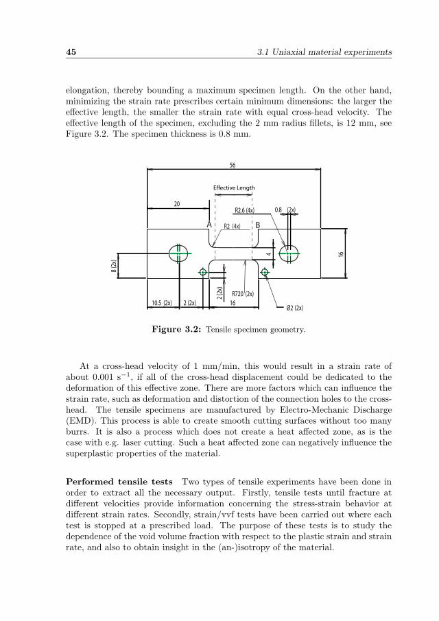
45 3.1 Uniaxial material experiments
elongation, thereby bounding a maximum specimen length. On the other hand,minimizing the strain rate prescribes certain minimum dimensions: the larger theeffective length, the smaller the strain rate with equal cross-head velocity. Theeffective length of the specimen, excluding the 2 mm radius fillets, is 12 mm, seeFigure 3.2. The specimen thickness is 0.8 mm.
4
R720 (2x)
56
16
10.5 (2x)
8(2
x)
16
2(2
x)
2 (2x)
R2.6 (4x)
Ø2 (2x)
20
R2 (4x)
0.8 (2x)
Effective Length
A B
Figure 3.2: Tensile specimen geometry.
At a cross-head velocity of 1 mm/min, this would result in a strain rate ofabout 0.001 s−1, if all of the cross-head displacement could be dedicated to thedeformation of this effective zone. There are more factors which can influence thestrain rate, such as deformation and distortion of the connection holes to the cross-head. The tensile specimens are manufactured by Electro-Mechanic Discharge(EMD). This process is able to create smooth cutting surfaces without too manyburrs. It is also a process which does not create a heat affected zone, as is thecase with e.g. laser cutting. Such a heat affected zone can negatively influence thesuperplastic properties of the material.
Performed tensile tests Two types of tensile experiments have been done inorder to extract all the necessary output. Firstly, tensile tests until fracture atdifferent velocities provide information concerning the stress-strain behavior atdifferent strain rates. Secondly, strain/vvf tests have been carried out where eachtest is stopped at a prescribed load. The purpose of these tests is to study thedependence of the void volume fraction with respect to the plastic strain and strainrate, and also to obtain insight in the (an-)isotropy of the material.
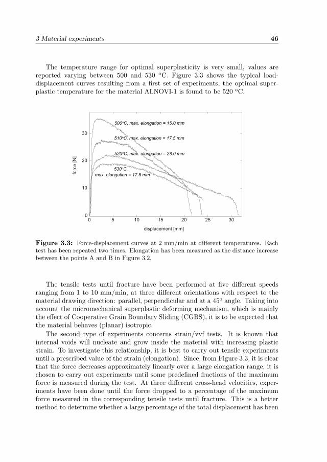
3 Material experiments 46
The temperature range for optimal superplasticity is very small, values arereported varying between 500 and 530 oC. Figure 3.3 shows the typical load-displacement curves resulting from a first set of experiments, the optimal super-plastic temperature for the material ALNOVI-1 is found to be 520 oC.
0 5 10 15 20 25 30 0
10
20
30
forc
e [N
]
displacement [mm]
500 oC, max. elongation = 15.0 mm
510 oC, max. elongation = 17.5 mm
530 oC, max. elongation = 17.8 mm
520 oC, max. elongation = 28.0 mm
Figure 3.3: Force-displacement curves at 2 mm/min at different temperatures. Eachtest has been repeated two times. Elongation has been measured as the distance increasebetween the points A and B in Figure 3.2.
The tensile tests until fracture have been performed at five different speedsranging from 1 to 10 mm/min, at three different orientations with respect to thematerial drawing direction: parallel, perpendicular and at a 45o angle. Taking intoaccount the micromechanical superplastic deforming mechanism, which is mainlythe effect of Cooperative Grain Boundary Sliding (CGBS), it is to be expected thatthe material behaves (planar) isotropic.
The second type of experiments concerns strain/vvf tests. It is known thatinternal voids will nucleate and grow inside the material with increasing plasticstrain. To investigate this relationship, it is best to carry out tensile experimentsuntil a prescribed value of the strain (elongation). Since, from Figure 3.3, it is clearthat the force decreases approximately linearly over a large elongation range, it ischosen to carry out experiments until some predefined fractions of the maximumforce is measured during the test. At three different cross-head velocities, exper-iments have been done until the force dropped to a percentage of the maximumforce measured in the corresponding tensile tests until fracture. This is a bettermethod to determine whether a large percentage of the total displacement has been
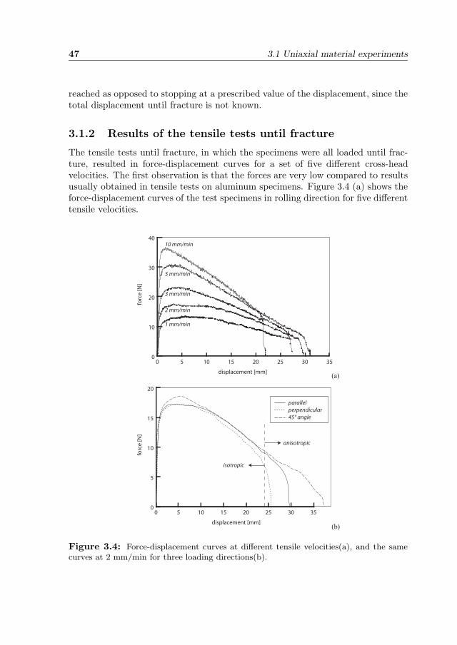
47 3.1 Uniaxial material experiments
reached as opposed to stopping at a prescribed value of the displacement, since thetotal displacement until fracture is not known.
3.1.2 Results of the tensile tests until fracture
The tensile tests until fracture, in which the specimens were all loaded until frac-ture, resulted in force-displacement curves for a set of five different cross-headvelocities. The first observation is that the forces are very low compared to resultsusually obtained in tensile tests on aluminum specimens. Figure 3.4 (a) shows theforce-displacement curves of the test specimens in rolling direction for five differenttensile velocities.
0 5 10 15 20 25 30 350
10
20
30
40
displacement [mm]
forc
e [N
]
1 mm/min
2 mm/min
3 mm/min
5 mm/min
10 mm/min
(a)
0 5 10 15 20 25 30 350
5
10
15
20
displacement [mm]
forc
e [N
]
parallelperpendicular45° angle
(b)
isotropic
anisotropic
Figure 3.4: Force-displacement curves at different tensile velocities(a), and the samecurves at 2 mm/min for three loading directions(b).
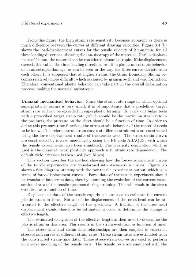
3 Material experiments 48
From this figure, the high strain rate sensitivity becomes apparent as there ismuch difference between the curves at different drawing velocities. Figure 3.4 (b)shows the load-displacement curves for the tensile velocity of 2 mm/min, for allthree loading directions, showing the (an-)isotropy of the material. Until a displace-ment of 24 mm, the material can be considered planar isotropic. If the displacementexceeds this value, the three loading directions result in planar anisotropic behavioror in anisotropic damage, as can be seen in the way the three curves deviate fromeach other. It is supposed that at higher strains, the Grain Boundary Sliding be-comes relatively more difficult, which is caused by grain growth and void formation.Therefore, conventional plastic behavior can take part in the overall deformationprocess, making the material anisotropic.
Uniaxial mechanical behavior Since the strain rate range in which optimalsuperplasticity occurs is very small, it is of importance that a predefined targetstrain rate will not be exceeded in superplastic forming. To carry out bulge testswith a prescribed target strain rate (which should be the maximum strain rate inthe product), the pressure on the sheet should be a function of time. In order todefine this pressure-time function, the stress-strain behavior of the material needsto be known. Therefore, stress-strain curves at different strain rates are constructedusing the force-displacement results of the tensile tests. The stress-strain curvesare constructed by inverse modeling by using the FE code ABAQUS, with whichthe tensile experiments have been simulated. The plasticity description which isused is the classical metal plasticity approach with strain rate dependency. Thedefault yield criterion is then used (von Mises).
This section describes the method showing how the force-displacement curvesof the tensile experiments are transformed into stress-strain curves. Figure 3.5shows a flow diagram, starting with the raw tensile experiment output, which is interms of force-displacement curves. Force data of the tensile experiment shouldbe translated into stress data, thereby assuming the evolution of the current cross-sectional area of the tensile specimen during straining. This will result in the stressevolution as a function of time.
Displacement data of the tensile experiment are used to estimate the currentplastic strain in time. Not all of the displacement of the cross-head can be at-tributed to the effective length of the specimen. A fraction of the cross-headdisplacement should therefore be estimated in order to determine the change ineffective length.
The estimated elongation of the effective length is then used to determine theplastic strain in this area. This results in the strain evolution as function of time.
The stress-time and strain-time relationships are then coupled to constructstress-strain curves at different strain rates. These strain rates are estimated fromthe constructed strain-time data. These stress-strain curves are used to performan inverse modeling of the tensile tests. The tensile tests are simulated with the
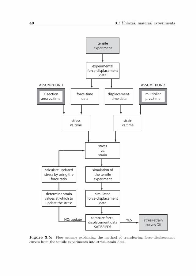
49 3.1 Uniaxial material experiments
ASSUMPTION 1 ASSUMPTION 2
stress-straincurves OK
stressvs. time
strainvs. time
X-sectionarea vs. time
force-timedata
displacement-time data
multiplierμ vs. time
simulatedforce-displacement
data
simulation ofthe tensile
experiment
stressvs.
strain
compare force-displacement data
SATISFIED?
experimentalforce-displacement
data
tensileexperiment
YESNO: update
determine strainvalues at which toupdate the stress
calculate updatedstress by using the
force ratio
Figure 3.5: Flow scheme explaining the method of transferring force-displacementcurves from the tensile experiments into stress-strain data.
3 Material experiments 50
constructed stress-strain data, where the output of these simulations is in terms offorce versus displacement.
The simulated force-displacement output is compared with the one measured inthe experiments. The deviation between both is used to improve the stress-strainbehavior. This is done as follows. The tensile force at ten points on the simulatedforce-displacement curve is compared with the experimentally determined force atthe same displacement. The strain at this displacement is then derived. The up-dated stress at this strain is then determined by multiplying the old stress value bythe ratio between the experimentally and simulation-based force. This procedureis repeated until sufficient correspondence between the experiment and the simu-lation will be reached, by minimizing the RMS value between both curves at theseten points.
To estimate the stress in the tensile specimen as a function of the time, thecurrent cross-sectional area evolution must either be known, or be estimated. Sinceit was not possible to monitor the width and thickness of the specimen during atensile test (because of the surrounding tunnel furnace), the cross-sectional areamust be estimated. The width and the thickness were measured at the start andthe end of an experiment. The initial assumption of the cross-sectional evolution issuch that both width and thickness decrease linearly with displacement (or time,since the cross-head velocity is constant). Then both the force and the estimatedcross-sectional area with time are known, so the estimated stress as a function oftime is known. Volume preservation is not checked here, since the goal of thisprocedure is only to obtain a first estimate of the stress-strain behavior.
The estimate of the plastic strain is somewhat more complicated, a few as-sumptions are made here. Since the flow stress is very low, it is assumed that all ofthe calculated strain can be considered plastic. The length of the effective zone isassumed to be 35% of the total distance between the hole centers of the specimen,which is based on a purely elastic simulation. This fraction is taken as a start-ing value μ0 at zero displacement, which increases with increasing strain. Also afirst simulation, where only elasticity is considered, shows that initially about thisfraction of the total displacement can be attributed to the effective zone.
This multiplier μx, which is initially 0.35, will increase with the overall displace-ment. Generally, in tensile experiments, the strain rate decreases with increasingelongation, provided that the cross-head velocity is constant. However, in thiscase, the strain rate is assumed constant, because μx increases with increasingelongation. If the drawing velocity is v [mm/s], then the strain rate is
ε =μ0v
l0(3.1)
where l0 is the initial effective length, and μ0 is the initial value of the multiplier.At the lowest tensile velocity, which is 1 mm/min, this results in an initial strainrate of 4.9·10−4 s−1.
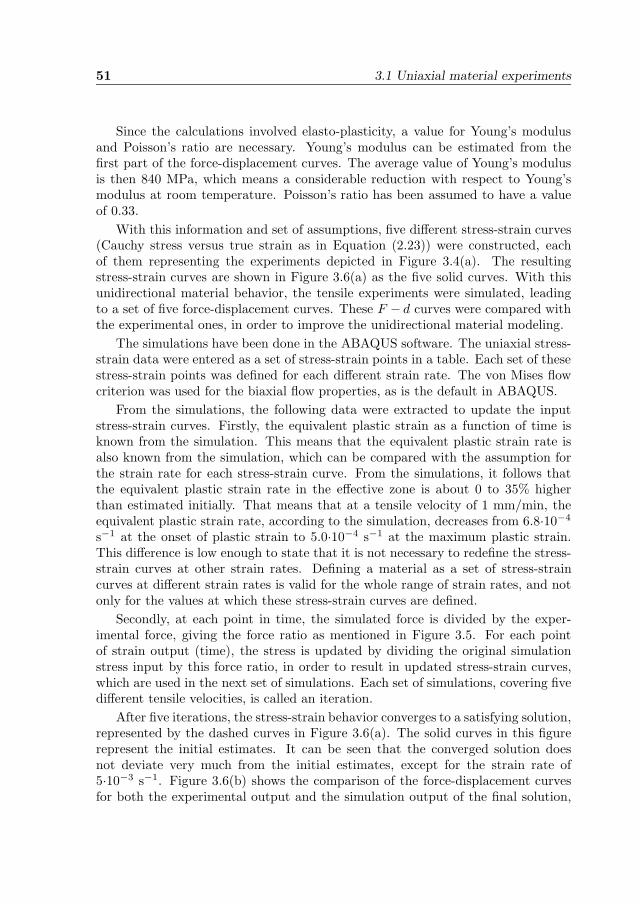
51 3.1 Uniaxial material experiments
Since the calculations involved elasto-plasticity, a value for Young’s modulusand Poisson’s ratio are necessary. Young’s modulus can be estimated from thefirst part of the force-displacement curves. The average value of Young’s modulusis then 840 MPa, which means a considerable reduction with respect to Young’smodulus at room temperature. Poisson’s ratio has been assumed to have a valueof 0.33.
With this information and set of assumptions, five different stress-strain curves(Cauchy stress versus true strain as in Equation (2.23)) were constructed, eachof them representing the experiments depicted in Figure 3.4(a). The resultingstress-strain curves are shown in Figure 3.6(a) as the five solid curves. With thisunidirectional material behavior, the tensile experiments were simulated, leadingto a set of five force-displacement curves. These F − d curves were compared withthe experimental ones, in order to improve the unidirectional material modeling.
The simulations have been done in the ABAQUS software. The uniaxial stress-strain data were entered as a set of stress-strain points in a table. Each set of thesestress-strain points was defined for each different strain rate. The von Mises flowcriterion was used for the biaxial flow properties, as is the default in ABAQUS.
From the simulations, the following data were extracted to update the inputstress-strain curves. Firstly, the equivalent plastic strain as a function of time isknown from the simulation. This means that the equivalent plastic strain rate isalso known from the simulation, which can be compared with the assumption forthe strain rate for each stress-strain curve. From the simulations, it follows thatthe equivalent plastic strain rate in the effective zone is about 0 to 35% higherthan estimated initially. That means that at a tensile velocity of 1 mm/min, theequivalent plastic strain rate, according to the simulation, decreases from 6.8·10−4
s−1 at the onset of plastic strain to 5.0·10−4 s−1 at the maximum plastic strain.This difference is low enough to state that it is not necessary to redefine the stress-strain curves at other strain rates. Defining a material as a set of stress-straincurves at different strain rates is valid for the whole range of strain rates, and notonly for the values at which these stress-strain curves are defined.
Secondly, at each point in time, the simulated force is divided by the exper-imental force, giving the force ratio as mentioned in Figure 3.5. For each pointof strain output (time), the stress is updated by dividing the original simulationstress input by this force ratio, in order to result in updated stress-strain curves,which are used in the next set of simulations. Each set of simulations, covering fivedifferent tensile velocities, is called an iteration.
After five iterations, the stress-strain behavior converges to a satisfying solution,represented by the dashed curves in Figure 3.6(a). The solid curves in this figurerepresent the initial estimates. It can be seen that the converged solution doesnot deviate very much from the initial estimates, except for the strain rate of5·10−3 s−1. Figure 3.6(b) shows the comparison of the force-displacement curvesfor both the experimental output and the simulation output of the final solution,
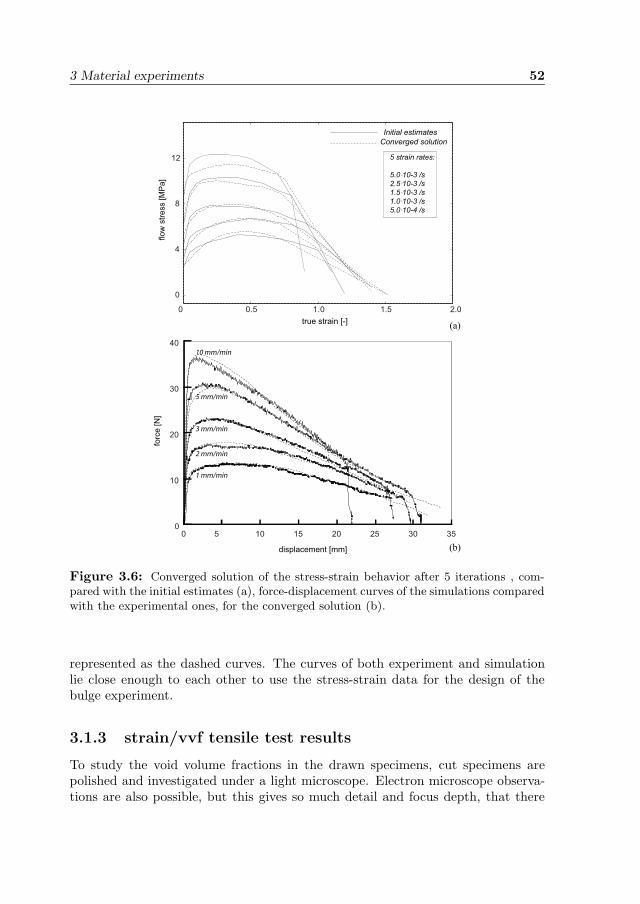
3 Material experiments 52
0 0.5 1.0 1.5 2.0
0
4
8
12
Converged solutionInitial estimates
true strain [-]
flow
str
ess [M
Pa]
5 strain rates:
5.0 10-3 /s2.5 10-3 /s1.5 10-3 /s1.0 10-3 /s5.0 10-4 /s
0 5 10 15 20 25 30 350
10
20
30
40
displacement [mm]
forc
e [N
]
1 mm/min
2 mm/min
3 mm/min
5 mm/min
10 mm/min
(a)
(b)
.
.
.
.
.
Figure 3.6: Converged solution of the stress-strain behavior after 5 iterations , com-pared with the initial estimates (a), force-displacement curves of the simulations comparedwith the experimental ones, for the converged solution (b).
represented as the dashed curves. The curves of both experiment and simulationlie close enough to each other to use the stress-strain data for the design of thebulge experiment.
3.1.3 strain/vvf tensile test results
To study the void volume fractions in the drawn specimens, cut specimens arepolished and investigated under a light microscope. Electron microscope observa-tions are also possible, but this gives so much detail and focus depth, that there
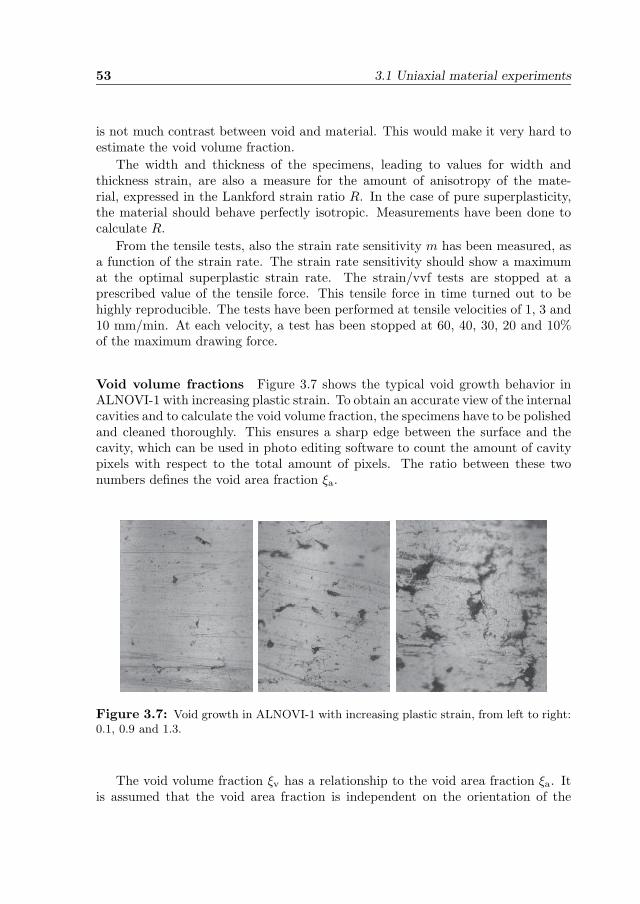
53 3.1 Uniaxial material experiments
is not much contrast between void and material. This would make it very hard toestimate the void volume fraction.
The width and thickness of the specimens, leading to values for width andthickness strain, are also a measure for the amount of anisotropy of the mate-rial, expressed in the Lankford strain ratio R. In the case of pure superplasticity,the material should behave perfectly isotropic. Measurements have been done tocalculate R.
From the tensile tests, also the strain rate sensitivity m has been measured, asa function of the strain rate. The strain rate sensitivity should show a maximumat the optimal superplastic strain rate. The strain/vvf tests are stopped at aprescribed value of the tensile force. This tensile force in time turned out to behighly reproducible. The tests have been performed at tensile velocities of 1, 3 and10 mm/min. At each velocity, a test has been stopped at 60, 40, 30, 20 and 10%of the maximum drawing force.
Void volume fractions Figure 3.7 shows the typical void growth behavior inALNOVI-1 with increasing plastic strain. To obtain an accurate view of the internalcavities and to calculate the void volume fraction, the specimens have to be polishedand cleaned thoroughly. This ensures a sharp edge between the surface and thecavity, which can be used in photo editing software to count the amount of cavitypixels with respect to the total amount of pixels. The ratio between these twonumbers defines the void area fraction ξa.
Figure 3.7: Void growth in ALNOVI-1 with increasing plastic strain, from left to right:0.1, 0.9 and 1.3.
The void volume fraction ξv has a relationship to the void area fraction ξa. Itis assumed that the void area fraction is independent on the orientation of the
3 Material experiments 54
observed plane. This means that
(1 − ξa)3/2 = (1 − ξv) (3.2)
orξv = 1 − (1 − ξa)3/2 (3.3)
In Figure 3.8, the measured void volume fractions are presented as a function ofthe equivalent plastic strain for different strain rates, compared e.g. with [21].
0.0 0.2 0.4 0.6 0.8 1.0 1.20
3
6
9
12
equivalent plastic strain [-]
vo
id v
olu
me
fra
ctio
n [%
]
ε = 5.0 .10 −4 /sε = 1.5 .10 −3 /sε = 5. 0 .10 −3 /s
Figure 3.8: Void volume fractions as measured from the strain/vvf tensile experiments.The dashed lines mark the bounds of the measurements.
Firstly, as was also shown qualitatively in Figure 3.7, it was observed that thevoid volume fraction increases with increasing plastic strain. Secondly, the voidvolume fraction shows hardly any dependence on the strain rate, see also [13].Thirdly, it seems that there exists a value for the plastic strain εtr (a transitionstrain), where the void volume fraction rate increases instantly, from ξ1 to ξ2 (orfrom slope c1 to c2). This can be explained by the fact that at higher plastic strains,the grains inside the material cannot accommodate enough to provide a smoothGrain Boundary Sliding process.
Lankford strain ratio From all the deformed specimens in the strain/vvf testseries, the resulting width and thickness were measured. By using the initial widthand thickness, the plastic strains in these directions were calculated. The Lankfordstrain ratio is determined as the strain in width direction divided by the thicknessstrain in a uniaxial experiment. A value less than 1, which is common for alu-minum alloys, means that the absolute value plastic thickness strain is higher than
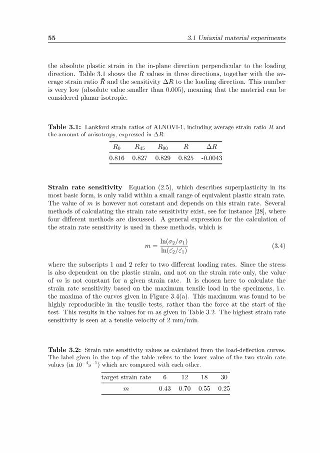
55 3.1 Uniaxial material experiments
the absolute plastic strain in the in-plane direction perpendicular to the loadingdirection. Table 3.1 shows the R values in three directions, together with the av-erage strain ratio R and the sensitivity ΔR to the loading direction. This numberis very low (absolute value smaller than 0.005), meaning that the material can beconsidered planar isotropic.
Table 3.1: Lankford strain ratios of ALNOVI-1, including average strain ratio R andthe amount of anisotropy, expressed in ΔR.
R0 R45 R90 R ΔR
0.816 0.827 0.829 0.825 -0.0043
Strain rate sensitivity Equation (2.5), which describes superplasticity in itsmost basic form, is only valid within a small range of equivalent plastic strain rate.The value of m is however not constant and depends on this strain rate. Severalmethods of calculating the strain rate sensitivity exist, see for instance [28], wherefour different methods are discussed. A general expression for the calculation ofthe strain rate sensitivity is used in these methods, which is
m =ln(σ2/σ1)ln(ε2/ε1)
(3.4)
where the subscripts 1 and 2 refer to two different loading rates. Since the stressis also dependent on the plastic strain, and not on the strain rate only, the valueof m is not constant for a given strain rate. It is chosen here to calculate thestrain rate sensitivity based on the maximum tensile load in the specimens, i.e.the maxima of the curves given in Figure 3.4(a). This maximum was found to behighly reproducible in the tensile tests, rather than the force at the start of thetest. This results in the values for m as given in Table 3.2. The highest strain ratesensitivity is seen at a tensile velocity of 2 mm/min.
Table 3.2: Strain rate sensitivity values as calculated from the load-deflection curves.The label given in the top of the table refers to the lower value of the two strain ratevalues (in 10−4s−1) which are compared with each other.
target strain rate 6 12 18 30
m 0.43 0.70 0.55 0.25
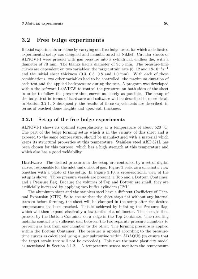
3 Material experiments 56
3.2 Free bulge experiments
Biaxial experiments are done by carrying out free bulge tests, for which a dedicatedexperimental setup was designed and manufactured at Nikhef. Circular sheets ofALNOVI-1 were pressed with gas pressure into a cylindrical, endless die, with adiameter of 70 mm. The blanks had a diameter of 95.5 mm. The pressure-timecurves are dependent on two variables: the target strain rate (6, 12 and 18·10−4s−1
and the initial sheet thickness (0.3, 0.5, 0.8 and 1.0 mm). With each of thesecombinations, two other variables had to be controlled: the maximum duration ofeach test and the applied backpressure during the test. A program was developedwithin the software LabVIEW to control the pressures on both sides of the sheetin order to follow the pressure-time curves as closely as possible. The setup ofthe bulge test in terms of hardware and software will be described in more detailin Section 3.2.1. Subsequently, the results of these experiments are described, interms of reached dome heights and apex wall thickness.
3.2.1 Setup of the free bulge experiments
ALNOVI-1 shows its optimal superplasticity at a temperature of about 520 oC.The part of the bulge forming setup which is in the vicinity of this sheet and isexposed to the same temperature, should be manufactured with a material whichkeeps its structural properties at this temperature. Stainless steel AISI 321L hasbeen chosen for this purpose, which has a high strength at this temperature andwhich also has a good weldability.
Hardware The desired pressures in the setup are controlled by a set of digitalvalves, responsible for the inlet and outlet of gas. Figure 3.9 shows a schematic viewtogether with a photo of the setup. In Figure 3.10, a cross-sectional view of thesetup is shown. Three pressure vessels are present, a Top and a Bottom Container,and a Pressure Bag. Because the volumes of Top and Bottom are small, they areartificially increased by applying two buffer cylinders (CYL).
The aluminum sheet and the stainless steel have a different Coefficient of Ther-mal Expansion (CTE). So to ensure that the sheet stays flat without any internalstresses before forming, the sheet will be clamped in the setup after the desiredtemperature has been reached. This is achieved by inflating the Pressure Bag,which will then expand elastically a few tenths of a millimeter. The sheet is thenpressed by the Bottom Container on a ridge in the Top Container. The resultingmetallic contact is a sufficient seal between the two separate pressure chambers toprevent gas leak from one chamber to the other. The forming pressure is appliedwithin the Bottom Container. The pressure is applied according to the pressure-time curves as calculated using a user subroutine within ABAQUS (to ensure thatthe target strain rate will not be exceeded). This uses the same plasticity modelas mentioned in Section 3.1.2. A temperature sensor monitors the temperature
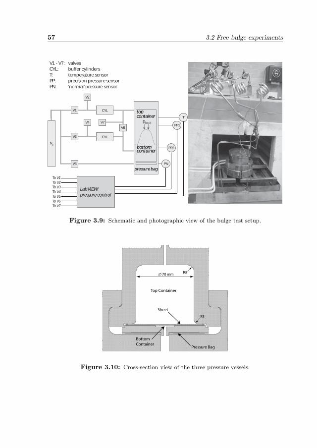
57 3.2 Free bulge experiments
V1 - V7: valvesCYL: buffer cylindersT: temperature sensorPP: precision pressure sensorPN: ‘normal’ pressure sensor
pressure bag
bottomcontainer
topcontainer
pform
pback
N2
V1
V2
V5
CYL
CYL
PP1
PP2
PN
LabVIEW: pressure control
T
To V1To V2To V3To V4To V5To V6To V7
V3
V6
V7V4
Figure 3.9: Schematic and photographic view of the bulge test setup.
Top Container
Bottom Container
Pressure Bag
Sheet
70 mm R8
R5
Figure 3.10: Cross-section view of the three pressure vessels.
3 Material experiments 58
of the containers together with the sheet. This temperature is controlled withan extra band heater surrounding the containers. Without this band heater, thefluctuations in temperature caused by the thermostat of the furnace are too high.With this band, the temperature fluctuations are within 1 oC deviation from thetarget temperature.
Software The bulge test is controlled by a program written in LabVIEW, whichuses a temperature and three pressure readouts as input, and seven digital valvepositions as output. A NI-DAQPad-6015 from National Instruments is used for thedata transport from the setup to LabVIEW and vice versa.
The necessary input in this program are the target strain rate, the backpressureto be applied during the test and a time limit (i.e. duration of the test). A fixedsequence of steps is followed to obtain a properly formed cup. The detailed sequenceof steps is written out in Appendix A.
3.2.2 Pressure control
If a superplastic aluminum sheet is deformed at its optimal superplastic tempera-ture, control over the maximum strain rate is necessary. Exposing the material fora long time to a high temperature will result, however, in losing superplastic prop-erties, so the deforming time should be as small as possible. Hence, the optimal wayto deform a sheet is by taking care that at each time point, this maximum strainrate will be reached. This can be achieved by prescribing the forming pressure asa function of time [31, 48].
During the whole forming process, the maximum strain rate may not exceed apredefined target strain rate. In a nonlinear simulation, this can be achieved byprescribing the pressure load in the current time increment depending on the max-imum strain rate in the process in the previous time increment. A self-developeduser subroutine which was provided with the simulation reads the equivalent plas-tic strain rate at each increment at each element. This strain rate in the modelis then compared with the target strain rate. The pressure increase or decreaseon the sheet in the next increment is then a function of the ratio between themaximum equivalent plastic strain rate in the model and the target strain rate. Ifthe maximum equivalent plastic strain rate is higher, respectively lower than thetarget strain rate, then the pressure will be multiplied by a value less, respectivelymore than 1. To prevent sudden increases and decreases at each successive timeincrement, this multiplication factor equals 1 in a small zone between 0.9 and 1.1times the ratio between maximum and target strain rate. The multiplication factoris always ’damped’, also to prevent sudden pressure changes due to element strainrate changes that are too severe.
The FE model consists of a quarter of a sheet, with symmetry boundary con-ditions applied on both symmetry edges. The sheet has been meshed with 3410
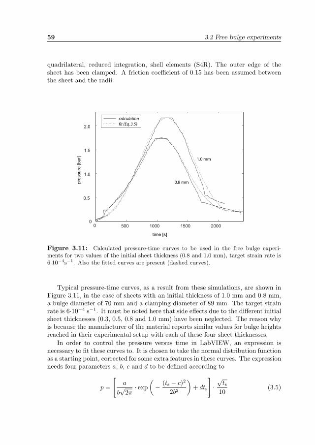
59 3.2 Free bulge experiments
quadrilateral, reduced integration, shell elements (S4R). The outer edge of thesheet has been clamped. A friction coefficient of 0.15 has been assumed betweenthe sheet and the radii.
0 500 1000 1500 2000
0
0.5
1.0
1.5
2.0
time [s]
pre
ssu
re [b
ar] 1.0 mm
0.8 mm
calculationfit (Eq. 3.5)
Figure 3.11: Calculated pressure-time curves to be used in the free bulge experi-ments for two values of the initial sheet thickness (0.8 and 1.0 mm), target strain rate is6·10−4s−1. Also the fitted curves are present (dashed curves).
Typical pressure-time curves, as a result from these simulations, are shown inFigure 3.11, in the case of sheets with an initial thickness of 1.0 mm and 0.8 mm,a bulge diameter of 70 mm and a clamping diameter of 89 mm. The target strainrate is 6·10−4 s−1. It must be noted here that side effects due to the different initialsheet thicknesses (0.3, 0.5, 0.8 and 1.0 mm) have been neglected. The reason whyis because the manufacturer of the material reports similar values for bulge heightsreached in their experimental setup with each of these four sheet thicknesses.
In order to control the pressure versus time in LabVIEW, an expression isnecessary to fit these curves to. It is chosen to take the normal distribution functionas a starting point, corrected for some extra features in these curves. The expressionneeds four parameters a, b, c and d to be defined according to
p =
[a
b√
2π· exp
(− (ts − c)2
2b2
)+ dts
]·√
ts10
(3.5)
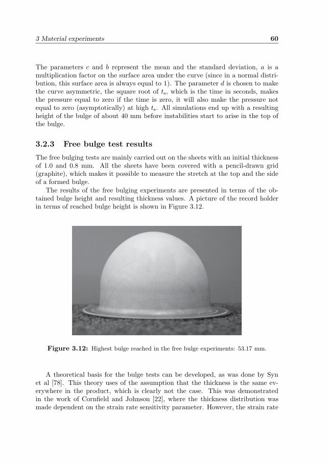
3 Material experiments 60
The parameters c and b represent the mean and the standard deviation, a is amultiplication factor on the surface area under the curve (since in a normal distri-bution, this surface area is always equal to 1). The parameter d is chosen to makethe curve asymmetric, the square root of ts, which is the time in seconds, makesthe pressure equal to zero if the time is zero, it will also make the pressure notequal to zero (asymptotically) at high ts. All simulations end up with a resultingheight of the bulge of about 40 mm before instabilities start to arise in the top ofthe bulge.
3.2.3 Free bulge test results
The free bulging tests are mainly carried out on the sheets with an initial thicknessof 1.0 and 0.8 mm. All the sheets have been covered with a pencil-drawn grid(graphite), which makes it possible to measure the stretch at the top and the sideof a formed bulge.
The results of the free bulging experiments are presented in terms of the ob-tained bulge height and resulting thickness values. A picture of the record holderin terms of reached bulge height is shown in Figure 3.12.
Figure 3.12: Highest bulge reached in the free bulge experiments: 53.17 mm.
A theoretical basis for the bulge tests can be developed, as was done by Synet al [78]. This theory uses of the assumption that the thickness is the same ev-erywhere in the product, which is clearly not the case. This was demonstratedin the work of Cornfield and Johnson [22], where the thickness distribution wasmade dependent on the strain rate sensitivity parameter. However, the strain rate
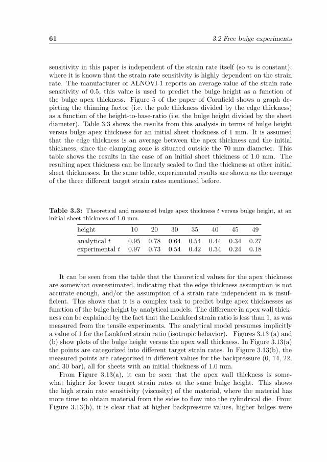
61 3.2 Free bulge experiments
sensitivity in this paper is independent of the strain rate itself (so m is constant),where it is known that the strain rate sensitivity is highly dependent on the strainrate. The manufacturer of ALNOVI-1 reports an average value of the strain ratesensitivity of 0.5, this value is used to predict the bulge height as a function ofthe bulge apex thickness. Figure 5 of the paper of Cornfield shows a graph de-picting the thinning factor (i.e. the pole thickness divided by the edge thickness)as a function of the height-to-base-ratio (i.e. the bulge height divided by the sheetdiameter). Table 3.3 shows the results from this analysis in terms of bulge heightversus bulge apex thickness for an initial sheet thickness of 1 mm. It is assumedthat the edge thickness is an average between the apex thickness and the initialthickness, since the clamping zone is situated outside the 70 mm-diameter. Thistable shows the results in the case of an initial sheet thickness of 1.0 mm. Theresulting apex thickness can be linearly scaled to find the thickness at other initialsheet thicknesses. In the same table, experimental results are shown as the averageof the three different target strain rates mentioned before.
Table 3.3: Theoretical and measured bulge apex thickness t versus bulge height, at aninitial sheet thickness of 1.0 mm.
height 10 20 30 35 40 45 49
analytical t 0.95 0.78 0.64 0.54 0.44 0.34 0.27experimental t 0.97 0.73 0.54 0.42 0.34 0.24 0.18
It can be seen from the table that the theoretical values for the apex thicknessare somewhat overestimated, indicating that the edge thickness assumption is notaccurate enough, and/or the assumption of a strain rate independent m is insuf-ficient. This shows that it is a complex task to predict bulge apex thicknesses asfunction of the bulge height by analytical models. The difference in apex wall thick-ness can be explained by the fact that the Lankford strain ratio is less than 1, as wasmeasured from the tensile experiments. The analytical model presumes implicitlya value of 1 for the Lankford strain ratio (isotropic behavior). Figures 3.13 (a) and(b) show plots of the bulge height versus the apex wall thickness. In Figure 3.13(a)the points are categorized into different target strain rates. In Figure 3.13(b), themeasured points are categorized in different values for the backpressure (0, 14, 22,and 30 bar), all for sheets with an initial thickness of 1.0 mm.
From Figure 3.13(a), it can be seen that the apex wall thickness is some-what higher for lower target strain rates at the same bulge height. This showsthe high strain rate sensitivity (viscosity) of the material, where the material hasmore time to obtain material from the sides to flow into the cylindrical die. FromFigure 3.13(b), it is clear that at higher backpressure values, higher bulges were
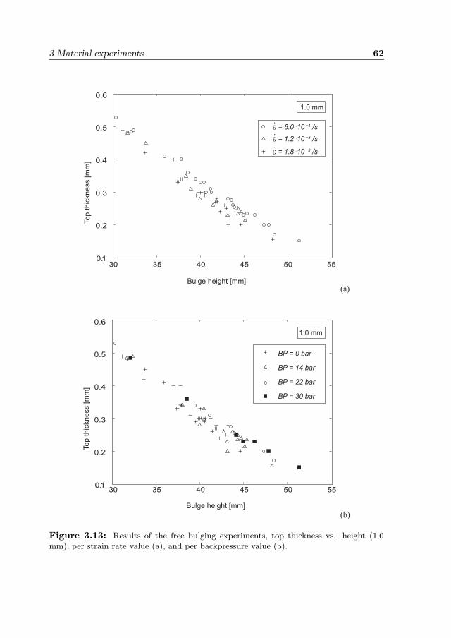
3 Material experiments 62
30 35 40 45 50 550.1
0.2
0.3
0.4
0.5
0.6
Bulge height [mm]
To
p th
ickn
ess [m
m]
ε = 6.0 .10 −4 /sε = 1.2 .10 −3 /s
ε = 1.8 .10 −3 /s
(a)
1.0 mm
30 35 40 45 50 55
Bulge height [mm]
To
p th
ickn
ess [m
m]
0.1
0.2
0.3
0.4
0.5
0.6
(b)
BP = 0 bar
BP = 14 bar
BP = 22 bar
BP = 30 bar
1.0 mm
Figure 3.13: Results of the free bulging experiments, top thickness vs. height (1.0mm), per strain rate value (a), and per backpressure value (b).
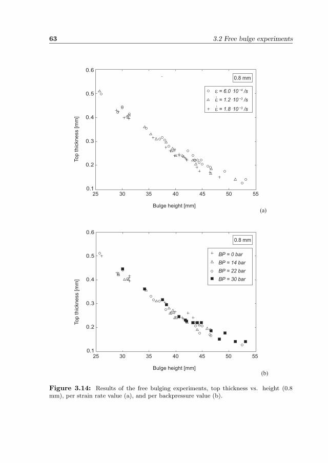
63 3.2 Free bulge experiments
25 30 35 40 45 50 55
Bulge height [mm]
To
p th
ickn
ess [m
m]
0.1
0.2
0.3
0.4
0.5
0.6
(a)
0.8 mm
25 30 35 40 45 50 55
Bulge height [mm]
To
p th
ickn
ess [m
m]
0.1
0.2
0.3
0.4
0.5
0.6
(b)
0.8 mm
BP = 0 barBP = 14 barBP = 22 barBP = 30 bar
ε = 6.0 .10 −4 /sε = 1.2 .10 −3 /s
ε = 1.8 .10 −3 /s
Figure 3.14: Results of the free bulging experiments, top thickness vs. height (0.8mm), per strain rate value (a), and per backpressure value (b).
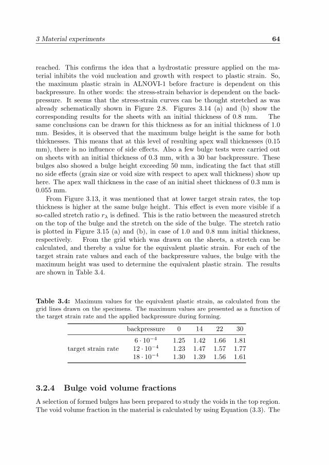
3 Material experiments 64
reached. This confirms the idea that a hydrostatic pressure applied on the ma-terial inhibits the void nucleation and growth with respect to plastic strain. So,the maximum plastic strain in ALNOVI-1 before fracture is dependent on thisbackpressure. In other words: the stress-strain behavior is dependent on the back-pressure. It seems that the stress-strain curves can be thought stretched as wasalready schematically shown in Figure 2.8. Figures 3.14 (a) and (b) show thecorresponding results for the sheets with an initial thickness of 0.8 mm. Thesame conclusions can be drawn for this thickness as for an initial thickness of 1.0mm. Besides, it is observed that the maximum bulge height is the same for boththicknesses. This means that at this level of resulting apex wall thicknesses (0.15mm), there is no influence of side effects. Also a few bulge tests were carried outon sheets with an initial thickness of 0.3 mm, with a 30 bar backpressure. Thesebulges also showed a bulge height exceeding 50 mm, indicating the fact that stillno side effects (grain size or void size with respect to apex wall thickness) show uphere. The apex wall thickness in the case of an initial sheet thickness of 0.3 mm is0.055 mm.
From Figure 3.13, it was mentioned that at lower target strain rates, the topthickness is higher at the same bulge height. This effect is even more visible if aso-called stretch ratio rλ is defined. This is the ratio between the measured stretchon the top of the bulge and the stretch on the side of the bulge. The stretch ratiois plotted in Figure 3.15 (a) and (b), in case of 1.0 and 0.8 mm initial thickness,respectively. From the grid which was drawn on the sheets, a stretch can becalculated, and thereby a value for the equivalent plastic strain. For each of thetarget strain rate values and each of the backpressure values, the bulge with themaximum height was used to determine the equivalent plastic strain. The resultsare shown in Table 3.4.
Table 3.4: Maximum values for the equivalent plastic strain, as calculated from thegrid lines drawn on the specimens. The maximum values are presented as a function ofthe target strain rate and the applied backpressure during forming.
backpressure 0 14 22 30
6 · 10−4 1.25 1.42 1.66 1.81target strain rate 12 · 10−4 1.23 1.47 1.57 1.77
18 · 10−4 1.30 1.39 1.56 1.61
3.2.4 Bulge void volume fractions
A selection of formed bulges has been prepared to study the voids in the top region.The void volume fraction in the material is calculated by using Equation (3.3). The
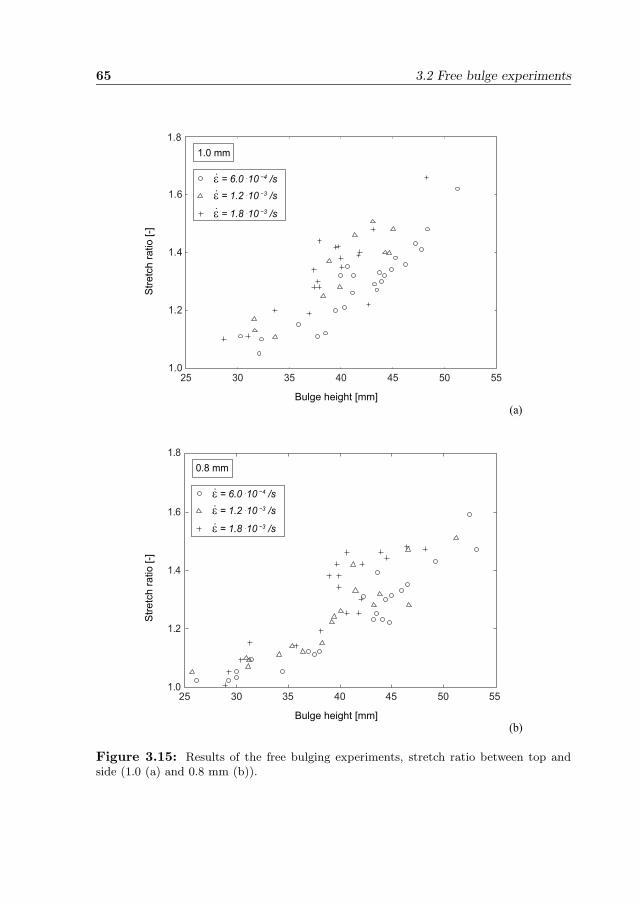
65 3.2 Free bulge experiments
25 30 35 40 45 50 551.0
1.2
1.4
1.6
Bulge height [mm]
Str
etc
h r
atio [-]
1.8
ε = 6.0 .10 −4 /sε = 1.2 .10 −3 /s
ε = 1.8 .10 −3 /s
(b)
0.8 mm
(a)
25 30 35 40 45 50 551.0
1.2
1.4
1.6
1.8
ε = 6.0 .10 −4 /sε = 1.2 .10 −3 /s
ε = 1.8 .10 −3 /s
1.0 mm
Bulge height [mm]
Str
etc
h r
atio [-]
Figure 3.15: Results of the free bulging experiments, stretch ratio between top andside (1.0 (a) and 0.8 mm (b)).
3 Material experiments 66
results of the observations are summarized in Figure 3.16. The expected trend isvisible, i.e. at higher backpressure values, the void volume fraction is lower at thesame bulge height. Therefore, higher bulges can be reached at higher backpressuresbefore failure of the material.
30 35 40 45 500
3
6
9
Vo
id v
olu
me
frac
tio
n [%
]
Bulge height [mm]
BP = 0 bar
BP = 14 bar
BP = 22 bar
BP = 30 bar
Figure 3.16: Void volume fractions of the top region of the bulges, categorized inbackpressure value. The dotted lines are drawn for a clearer view.
With the pencil drawn grid on the bulges, the stretch can be measured. Fromthe stretch, a value for the equivalent plastic strain can be calculated, taking intoaccount that on the top of the bulge an equibiaxial stress state is present. Table 3.5lists some values of the void volume fraction as function of the equivalent plasticstrain, in case no backpressure is applied.
Table 3.5: Void volume fractions as a function of the equivalent plastic strain, withoutthe application of a backpressure.
equivalent plastic strain 0.67 0.96 1.12 1.20
void volume fraction 1.3 2.5 6.1 9.1
If the values are compared with the void volume fraction observations from the
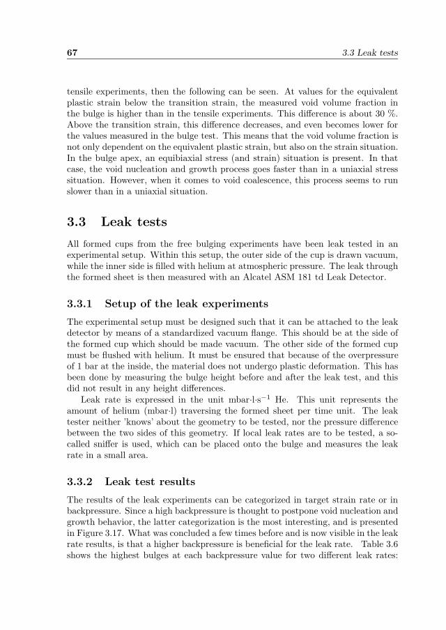
67 3.3 Leak tests
tensile experiments, then the following can be seen. At values for the equivalentplastic strain below the transition strain, the measured void volume fraction inthe bulge is higher than in the tensile experiments. This difference is about 30 %.Above the transition strain, this difference decreases, and even becomes lower forthe values measured in the bulge test. This means that the void volume fraction isnot only dependent on the equivalent plastic strain, but also on the strain situation.In the bulge apex, an equibiaxial stress (and strain) situation is present. In thatcase, the void nucleation and growth process goes faster than in a uniaxial stresssituation. However, when it comes to void coalescence, this process seems to runslower than in a uniaxial situation.
3.3 Leak tests
All formed cups from the free bulging experiments have been leak tested in anexperimental setup. Within this setup, the outer side of the cup is drawn vacuum,while the inner side is filled with helium at atmospheric pressure. The leak throughthe formed sheet is then measured with an Alcatel ASM 181 td Leak Detector.
3.3.1 Setup of the leak experiments
The experimental setup must be designed such that it can be attached to the leakdetector by means of a standardized vacuum flange. This should be at the side ofthe formed cup which should be made vacuum. The other side of the formed cupmust be flushed with helium. It must be ensured that because of the overpressureof 1 bar at the inside, the material does not undergo plastic deformation. This hasbeen done by measuring the bulge height before and after the leak test, and thisdid not result in any height differences.
Leak rate is expressed in the unit mbar·l·s−1 He. This unit represents theamount of helium (mbar·l) traversing the formed sheet per time unit. The leaktester neither ’knows’ about the geometry to be tested, nor the pressure differencebetween the two sides of this geometry. If local leak rates are to be tested, a so-called sniffer is used, which can be placed onto the bulge and measures the leakrate in a small area.
3.3.2 Leak test results
The results of the leak experiments can be categorized in target strain rate or inbackpressure. Since a high backpressure is thought to postpone void nucleation andgrowth behavior, the latter categorization is the most interesting, and is presentedin Figure 3.17. What was concluded a few times before and is now visible in the leakrate results, is that a higher backpressure is beneficial for the leak rate. Table 3.6shows the highest bulges at each backpressure value for two different leak rates:
3 Material experiments 68
0 10 20 30 40 50
Bulge height [mm]
Leak
rate
[mb
ar l/
s]
10−8
10−6
10−4
10−2
100
(a)
1.0 mm
BP = 0 bar
BP = 14 bar
BP = 22 bar
BP = 30 bar
0 10 20 30 40 50
Bulge height [mm]
Leak
rate
[mb
ar l/
s]
10−8
10−6
10−4
10−2
100
(b)
0.8 mm
BP = 0 bar
BP = 14 bar
BP = 22 bar
BP = 30 bar
Figure 3.17: Leak test results of the formed cups, leak rate vs. bulge height, bybackpressure value, at an initial thickness of (a): 1.0 mm, and (b): 0.8 mm

69 3.4 Die bulge experiments
Table 3.6: Overview of the highest bulges with a leak rate as defined in the table,expressed in mm and mbar l/s, respectively. The bulge heights are presented as dependenton the applied backpressure (BP; in bar) and the initial sheet thickness, 0.8 and 1.0 mm.
BP 0 14 22 30
Leak 10−8 0.8 mm 31.31 34.47 39.23 44.821.0 mm 31.67 37.97 39.43 46.26
Leak 100 0.8 mm 37.97 40.04 46.50 49.241.0 mm 41.85 42.69 47.27 51.32
firstly, a leak rate just above the minimum rate which could be measured (10−8
mbar l/s); secondly, the highest value of the leak rate below 100 mbar l/s, sincethis is a value at which no holes are visible in the bulge.
If holes were visible, these bulges were not leak-tested, since this would resultin a absurdly high leak value. Bulges with visible holes were all categorized undera leak value of 100 mbar l/s. From this table it can be concluded, and was alsoexpected, that a higher backpressure has a beneficial effect on the leak rate.
3.4 Die bulge experiments
When a sheet is pressed into a die to obtain a predetermined shape, the resultinggeometry is dependent on the friction between sheet and die. This section describesa die design which is used for die bulge experiments, with the goal to obtain frictioninformation. A set of experiments was designed where three variables were used,of which two were also used in the free bulge experiments: the target strain rateand the backpressure applied during the deformation process. The third variableis the friction coefficient, which is unknown beforehand. The design of the die issuch that the ratio of resulting thicknesses at two points in the deformed sheetdetermines the value of the friction coefficient.
3.4.1 Friction in superplastic materials
Friction in superplastic forming processes has not been studied intensively, it iscovered in e.g. [18, 51]. Two superplastic aluminum alloys are studied here, AA5083and AA7475. The aim is to study the frictional behavior as a function of the targetstrain rate and the applied backpressure. Also, the difference between lubricationand non-lubrication was studied.
In the case of AA5083, the lowest friction coefficients were measured betweenthe sheet and a steel die by using graphite as lubrication. In this case, the friction
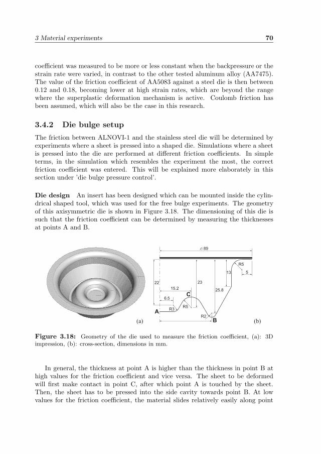
3 Material experiments 70
coefficient was measured to be more or less constant when the backpressure or thestrain rate were varied, in contrast to the other tested aluminum alloy (AA7475).The value of the friction coefficient of AA5083 against a steel die is then between0.12 and 0.18, becoming lower at high strain rates, which are beyond the rangewhere the superplastic deformation mechanism is active. Coulomb friction hasbeen assumed, which will also be the case in this research.
3.4.2 Die bulge setup
The friction between ALNOVI-1 and the stainless steel die will be determined byexperiments where a sheet is pressed into a shaped die. Simulations where a sheetis pressed into the die are performed at different friction coefficients. In simpleterms, in the simulation which resembles the experiment the most, the correctfriction coefficient was entered. This will be explained more elaborately in thissection under ’die bulge pressure control’.
Die design An insert has been designed which can be mounted inside the cylin-drical shaped tool, which was used for the free bulge experiments. The geometryof this axisymmetric die is shown in Figure 3.18. The dimensioning of this die issuch that the friction coefficient can be determined by measuring the thicknessesat points A and B.
(a) (b)
89
5
R5
13
25.8
R2
23
15.2
R5
6.5
R3
22
AB
C
Figure 3.18: Geometry of the die used to measure the friction coefficient, (a): 3Dimpression, (b): cross-section, dimensions in mm.
In general, the thickness at point A is higher than the thickness in point B athigh values for the friction coefficient and vice versa. The sheet to be deformedwill first make contact in point C, after which point A is touched by the sheet.Then, the sheet has to be pressed into the side cavity towards point B. At lowvalues for the friction coefficient, the material slides relatively easily along point
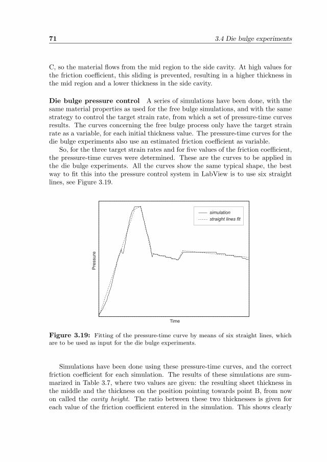
71 3.4 Die bulge experiments
C, so the material flows from the mid region to the side cavity. At high values forthe friction coefficient, this sliding is prevented, resulting in a higher thickness inthe mid region and a lower thickness in the side cavity.
Die bulge pressure control A series of simulations have been done, with thesame material properties as used for the free bulge simulations, and with the samestrategy to control the target strain rate, from which a set of pressure-time curvesresults. The curves concerning the free bulge process only have the target strainrate as a variable, for each initial thickness value. The pressure-time curves for thedie bulge experiments also use an estimated friction coefficient as variable.
So, for the three target strain rates and for five values of the friction coefficient,the pressure-time curves were determined. These are the curves to be applied inthe die bulge experiments. All the curves show the same typical shape, the bestway to fit this into the pressure control system in LabView is to use six straightlines, see Figure 3.19.
simulationstraight lines fit
Time
Pre
ssure
Figure 3.19: Fitting of the pressure-time curve by means of six straight lines, whichare to be used as input for the die bulge experiments.
Simulations have been done using these pressure-time curves, and the correctfriction coefficient for each simulation. The results of these simulations are sum-marized in Table 3.7, where two values are given: the resulting sheet thickness inthe middle and the thickness on the position pointing towards point B, from nowon called the cavity height. The ratio between these two thicknesses is given foreach value of the friction coefficient entered in the simulation. This shows clearly

3 Material experiments 72
Table 3.7: Mid and cavity height as a result from simulations where different values ofμ are entered. The ratio between these two thicknesses is also given.
μ 0.04 0.08 0.12 0.16 0.20
Mid thickness (mm) 0.181 0.228 0.244 0.259 0.268Cavity thickness (mm) 0.253 0.247 0.238 0.233 0.226
Thickness ratio 0.72 0.92 1.03 1.11 1.19
that the thickness ratio increases with increasing friction coefficient. The die bulgeexperiments are carried out using two lubricants: one series where graphite is used,these sheets have an initial thickness of 0.5 mm. The other series is lubricated witha mixture of graphite and molybdenum sulphide, called Molykote. The sheets lu-bricated with Molykote all have an initial thickness of 0.3 mm. This is expectedto be the thickness to be used for the forming of RF Foils, as is currently the case.Tests are performed either without the application of a backpressure, or with a 30bar backpressure.
3.4.3 Die bulge results
Figure 3.20 shows a picture of one of the formed sheets in the die bulge experiment.From all the sheets formed in this way, the following geometric properties weremeasured:
• the thickness in the middle of the sheet, this part of the sheet always touchesthe die (point A) in every performed test;
• the cavity height. In the experiments, point B was intentionally neverreached, because of the low fillet radius;
• the thickness at the cavity height. Compared with the thickness measuredin the middle of the formed sheet, this gives information about the frictioncoefficient;
• the leak value of the formed bulges.
Table 3.8 lists the average mid thickness, and the thickness at the cavity height ofthe series lubricated with graphite (0.5 mm initial thickness) as a function of thetarget strain rate. The maximum forming time is dependent on this target strainrate: 5400 seconds at 6·10−4 s−1, 2700 seconds at 12·10−4 s−1, and 1800 seconds at18·10−4 s−1. From the observations summarized in this table, no backpressure hasbeen applied during the forming process. Also, the average cavity height is listed inthe table. Table 3.9 shows the same observations, but now where a backpressure of
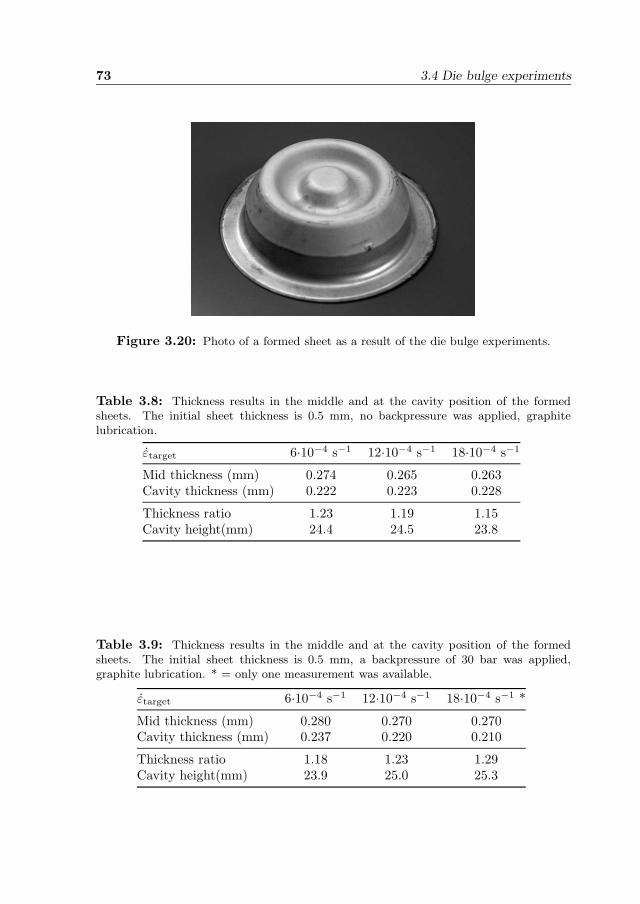
73 3.4 Die bulge experiments
Figure 3.20: Photo of a formed sheet as a result of the die bulge experiments.
Table 3.8: Thickness results in the middle and at the cavity position of the formedsheets. The initial sheet thickness is 0.5 mm, no backpressure was applied, graphitelubrication.
εtarget 6·10−4 s−1 12·10−4 s−1 18·10−4 s−1
Mid thickness (mm) 0.274 0.265 0.263Cavity thickness (mm) 0.222 0.223 0.228
Thickness ratio 1.23 1.19 1.15Cavity height(mm) 24.4 24.5 23.8
Table 3.9: Thickness results in the middle and at the cavity position of the formedsheets. The initial sheet thickness is 0.5 mm, a backpressure of 30 bar was applied,graphite lubrication. * = only one measurement was available.
εtarget 6·10−4 s−1 12·10−4 s−1 18·10−4 s−1 *
Mid thickness (mm) 0.280 0.270 0.270Cavity thickness (mm) 0.237 0.220 0.210
Thickness ratio 1.18 1.23 1.29Cavity height(mm) 23.9 25.0 25.3
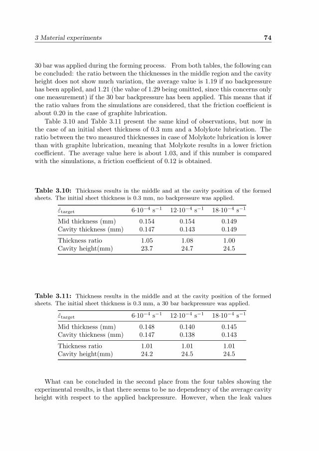
3 Material experiments 74
30 bar was applied during the forming process. From both tables, the following canbe concluded: the ratio between the thicknesses in the middle region and the cavityheight does not show much variation, the average value is 1.19 if no backpressurehas been applied, and 1.21 (the value of 1.29 being omitted, since this concerns onlyone measurement) if the 30 bar backpressure has been applied. This means that ifthe ratio values from the simulations are considered, that the friction coefficient isabout 0.20 in the case of graphite lubrication.
Table 3.10 and Table 3.11 present the same kind of observations, but now inthe case of an initial sheet thickness of 0.3 mm and a Molykote lubrication. Theratio between the two measured thicknesses in case of Molykote lubrication is lowerthan with graphite lubrication, meaning that Molykote results in a lower frictioncoefficient. The average value here is about 1.03, and if this number is comparedwith the simulations, a friction coefficient of 0.12 is obtained.
Table 3.10: Thickness results in the middle and at the cavity position of the formedsheets. The initial sheet thickness is 0.3 mm, no backpressure was applied.
εtarget 6·10−4 s−1 12·10−4 s−1 18·10−4 s−1
Mid thickness (mm) 0.154 0.154 0.149Cavity thickness (mm) 0.147 0.143 0.149
Thickness ratio 1.05 1.08 1.00Cavity height(mm) 23.7 24.7 24.5
Table 3.11: Thickness results in the middle and at the cavity position of the formedsheets. The initial sheet thickness is 0.3 mm, a 30 bar backpressure was applied.
εtarget 6·10−4 s−1 12·10−4 s−1 18·10−4 s−1
Mid thickness (mm) 0.148 0.140 0.145Cavity thickness (mm) 0.147 0.138 0.143
Thickness ratio 1.01 1.01 1.01Cavity height(mm) 24.2 24.5 24.5
What can be concluded in the second place from the four tables showing theexperimental results, is that there seems to be no dependency of the average cavityheight with respect to the applied backpressure. However, when the leak values
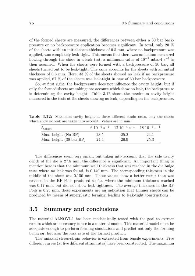
75 3.5 Summary and conclusions
of the formed sheets are measured, the differences between either a 30 bar back-pressure or no backpressure application becomes significant. In total, only 20 %of the sheets with an initial sheet thickness of 0.5 mm, where no backpressure wasapplied, was completely leak-tight. This means that there was no helium measuredflowing through the sheet in a leak test, a minimum value of 10−9 mbar·l s−1 isthen assumed. When the sheets were formed with a backpressure of 30 bar, allsheets turned out to be leak-tight. The same accounts for the sheets with an initialthickness of 0.3 mm. Here, 33 % of the sheets showed no leak if no backpressurewas applied, 67 % of the sheets was leak-tight in case of 30 bar backpressure.
So, at first sight, the backpressure does not influence the cavity height, but ifonly the formed sheets are taking into account which show no leak, the backpressureis determining the cavity height. Table 3.12 shows the maximum cavity heightmeasured in the tests at the sheets showing no leak, depending on the backpressure.
Table 3.12: Maximum cavity height at three different strain rates, only the sheetswhich show no leak are taken into account. Values are in mm.
εtarget 6·10−4 s−1 12·10−4 s−1 18·10−4 s−1
Max. height (No BP) 23.5 25.2 24.1Max. height (30 bar BP) 24.4 26.9 25.3
The differences seem very small, but taken into account that the side cavitydepth of the die is 27.8 mm, the difference is significant. An important thing tomention here is that the minimum wall thickness that was reached in the die bulgetests where no leak was found, is 0.140 mm. The corresponding thickness in themiddle of the sheet was 0.150 mm. These values show a better result than wasreached in the RF Foils produced so far, where the minimum thickness reachedwas 0.17 mm, but did not show leak tightness. The average thickness in the RFFoils is 0.25 mm, these experiments are an indication that thinner sheets can beproduced by means of superplastic forming, leading to leak-tight constructions.
3.5 Summary and conclusions
The material ALNOVI-1 has been mechanically tested with the goal to extractresults which are necessary to use in a material model. This material model must beadequate enough to perform forming simulations and predict not only the formingbehavior, but also the leak rate of the formed product.
The uniaxial stress-strain behavior is extracted from tensile experiments. Fivedifferent curves (at five different strain rates) have been constructed. The maximum

3 Material experiments 76
strain rate sensitivity (0.70) was measured to occur at the tensile specimens loadedat a cross-head velocity of 2 mm/min. This corresponds with a strain rate of12·10−4 s−1. The void volume fractions were measured, leading to a relationshipbetween this property and the plastic strain. This relationship shows a transitionin void growth rate. This growth rate has a lower value for plastic strains below atransition strain, and a higher value for plastic strains above this transition strain.The Lankford strain ratio was also measured, leading to a value of 0.825. Thisvalue is independent of the in-plane directions, so the material can be consideredplanar isotropic.
Free bulge experiments were carried out to study the forming behavior of thematerial. Void volume fractions and leak rates of the formed bulges were measured.These values are dependent on the applied backpressure during the forming pro-cess. The highest backpressure applied was 30 bar, which is a significant fractionof the flow stress of the material. Therefore, this backpressure postpones void nu-cleation/growth/coalescence, which means that a higher equivalent plastic straincan be reached without failure of the material. The highest bulge formed withoutthe application of a backpressure was 43 mm, whereas this height was 53 mm with30 bar backpressure applied. The highest bulges which can be considered almostleak-tight (leak rate is 10−8 mbar·l/s) were 31.67 mm without the backpressureapplied and 46.26 mm with 30 bar backpressure applied.
Die bulge experiments were performed to investigate the frictional behaviorbetween ALNOVI-1 and the material of the bulge setup (stainless steel AISI 321L).The friction coefficient was extracted by comparing two thickness values in theformed products. This resulted in a friction coefficient of 0.20 in the case of graphitelubrication and 0.12 in the case of Molykote lubrication. Also in these experiments,the leak rates were measured. The same conclusion as for the free bulge experimentscan be drawn: the application of a backpressure has a beneficial effect on the leakrate.
The data as resulted from the mechanical experiments described in this chapterwill be used to develop a constitutive model, to be used in superplastic formingsimulations. The development of this constitutive model is the subject of the nextchapter.
4. Superplastic material modeling
Finite element codes generally do not supply a superplastic material model, and ifone does, the formulation is comparable to the one mentioned in Equation (2.5),which is for instance used in the finite element software of MARC [26]. Dependingon the desired types of result and behavior to implement, it may be possible touse a predefined material type for the purpose of superplastic forming simulations.ABAQUS/Standard provides some material models in the class of metal plasticity,where isotropic or kinematic hardening can be combined with rate-dependent yield.
These material models are the subject of Section 4.1, together with a conclusionwhere the reasons are given for not using these models, thereby justifying the useof a user-defined material model (UMAT). This section also shows an evaluationof the use of the classical metal plasticity approach. This approach was used inSection 3.2.2 to predict the pressure-time curves for use in the bulge experiments.
The user-defined material model is described in this chapter, where the uniaxialbehavior is the subject of Section 4.2. The uniaxial stress-strain behavior, as pre-sented in Section 3.1 as a set of stress-strain curves at different plastic strain rates,is divided into three parts: the initial flow stress (at zero plastic strain), strainhardening behavior and the strain softening caused by internal void formation andgrowth. This section also describes the implementation of the pressure dependencyin the model.
The plane stress behavior, as a result of the free bulging experiments, is de-scribed in Section 4.3, where the Hosford flow criterion is recapitulated. Since thisflow criterion is expressed in the principal directions, an extra step is necessary inthe material model to translate the global stress vector into these directions.
As mentioned in Chapter 1, the most important constraint of an RF Shieldconcerns the leak tightness. To predict if a superplastically deformed sheet willsatisfy this constraint, this property should be added to the material model. Thisis the subject of Section 4.4.
The stress and necessary state variables should be updated every increment.Because this concerns in general a set of nonlinear equations to be solved, a Newtoniteration scheme is used in the user-defined material description to solve thesevariables. This procedure is described in Section 4.5.
77

4 Superplastic material modeling 78
4.1 ABAQUS material models
ABAQUS provides some sophisticated material models to simulate material plas-ticity. One class of plasticity models is the metal plasticity group, consisting of aclassical metal plasticity formulation, which can be extended by a set of additionalplasticity features. These features include for instance rate-dependent yield behav-ior or porosity effects. This section mentions firstly the built-in material models inABAQUS which may be suitable for the purpose of superplastic forming simula-tions or may provide useful information for building a user-defined material model.Secondly, the classical metal plasticity approach with strain-rate dependency willbe evaluated in this section.
4.1.1 Plasticity models
Three ABAQUS/Standard plasticity models were considered which could poten-tially be used in a superplastic constitutive model. However, all three have a fewlimitations, which prevented them from being used in this research project:
• the Porous Metal Plasticity model: It is based on Gurson’s porous metalplasticity theory together with a void nucleation definition. This model isvalid for void volume fractions not exceeding 10 %. The void volume fractionis calculated by means of an evolution law where the void growth is dependenton the current void volume fraction. The resulting void volume fraction isused to calculate the updated yield surface with respect to the yield surface incase no voids would be present. This model is only applicable to von Misesplasticity. The main problem is that this material type is not applicableto element types which assume a plane stress condition. This means thatto make use of this material type, three extra stress and strain componentswould be necessary by using e.g. volume elements. These components are notnecessary in sheet metal forming simulations and the use of volume elementsmay even lead to less accurate results and also to an unacceptable increasein computation time;
• the Drucker-Prager model: this model is generally used for granular-like ma-terials, which show different behavior in tension and compression, therebymaking the material dependent on the hydrostatic pressure. The microme-chanical deformation mechanism of superplastic materials can be consid-ered as particles (granules) sliding across each other, and is also pressure-dependent. However, the problem with this material type when using ele-ments with a plane stress formulation, is that a prescribed hydrostatic pres-sure cannot be applied. This means that there will be no difference in simula-tion results between applying the forming pressure only, and the applicationof a forming pressure in combination with a backpressure from the other sideof the sheet;
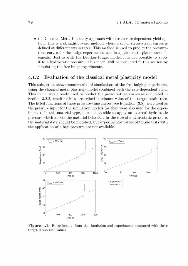
79 4.1 ABAQUS material models
• the Classical Metal Plasticity approach with strain-rate dependent yield op-tion: this is a straightforward method where a set of stress-strain curves isdefined at different strain rates. This method is used to predict the pressure-time curves for the bulge experiments, and is applicable to plane stress el-ements. Just as with the Drucker-Prager model, it is not possible to applyit to a hydrostatic pressure. This model will be evaluated in this section bysimulating the free bulge experiments.
4.1.2 Evaluation of the classical metal plasticity model
This subsection shows some results of simulations of the free bulging experiment,using the classical metal plasticity model combined with the rate-dependent yield.This model was already used to predict the pressure-time curves as calculated inSection 3.2.2, resulting in a prescribed maximum value of the target strain rate.The fitted functions of these pressure-time curves, see Equation (3.5), were used asthe pressure input for the simulation models (as they were also used for the exper-iments). In this material type, it is not possible to apply an external hydrostaticpressure which affects the material behavior. In the case of a hydrostatic pressure,the material data should be modified, but experimental values of tensile tests withthe application of a backpressure are not available.
0 300 600 900 1200 0
15
30
45
60
experimentsimulation
time [s]
bulg
e h
eig
ht [m
m]
0 150 300 450
0
15
30
45
60
time [s]
bulg
e h
eig
ht [m
m]
0 100 200 300 400 0
15
30
45
60
time [s]
bulg
e h
eig
ht [m
m]
εtarget = 6E-4 /s
εtarget = 18E-4 /s
εtarget = 12E-4 /s
Figure 4.1: Bulge heights from the simulation and experiments compared with threetarget strain rate values.
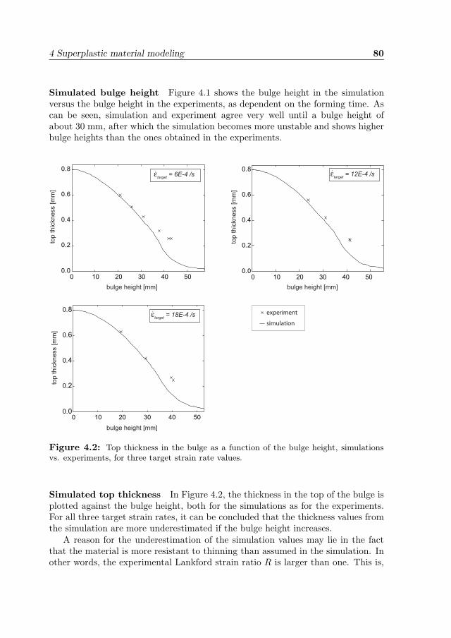
4 Superplastic material modeling 80
Simulated bulge height Figure 4.1 shows the bulge height in the simulationversus the bulge height in the experiments, as dependent on the forming time. Ascan be seen, simulation and experiment agree very well until a bulge height ofabout 30 mm, after which the simulation becomes more unstable and shows higherbulge heights than the ones obtained in the experiments.
0 10 20 30 40 500.0
0.2
0.4
0.6
0.8
bulge height [mm]
top
th
ickn
ess [
mm
]
0 10 20 30 40 500.0
0.2
0.4
0.6
0.8
bulge height [mm]
top
th
ickn
ess [
mm
]
0 10 20 30 40 500.0
0.2
0.4
0.6
0.8
bulge height [mm]
top
th
ickn
ess [
mm
]
εtarget = 6E-4 /s εtarget = 12E-4 /s
εtarget = 18E-4 /s experiment
simulation
Figure 4.2: Top thickness in the bulge as a function of the bulge height, simulationsvs. experiments, for three target strain rate values.
Simulated top thickness In Figure 4.2, the thickness in the top of the bulge isplotted against the bulge height, both for the simulations as for the experiments.For all three target strain rates, it can be concluded that the thickness values fromthe simulation are more underestimated if the bulge height increases.
A reason for the underestimation of the simulation values may lie in the factthat the material is more resistant to thinning than assumed in the simulation. Inother words, the experimental Lankford strain ratio R is larger than one. This is,
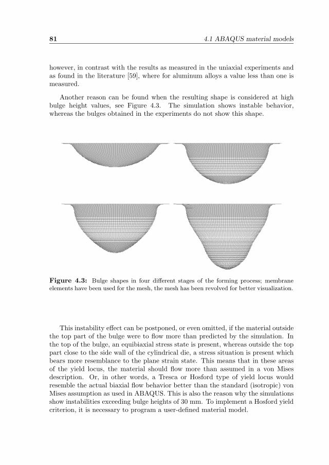
81 4.1 ABAQUS material models
however, in contrast with the results as measured in the uniaxial experiments andas found in the literature [59], where for aluminum alloys a value less than one ismeasured.
Another reason can be found when the resulting shape is considered at highbulge height values, see Figure 4.3. The simulation shows instable behavior,whereas the bulges obtained in the experiments do not show this shape.
Figure 4.3: Bulge shapes in four different stages of the forming process; membraneelements have been used for the mesh, the mesh has been revolved for better visualization.
This instability effect can be postponed, or even omitted, if the material outsidethe top part of the bulge were to flow more than predicted by the simulation. Inthe top of the bulge, an equibiaxial stress state is present, whereas outside the toppart close to the side wall of the cylindrical die, a stress situation is present whichbears more resemblance to the plane strain state. This means that in these areasof the yield locus, the material should flow more than assumed in a von Misesdescription. Or, in other words, a Tresca or Hosford type of yield locus wouldresemble the actual biaxial flow behavior better than the standard (isotropic) vonMises assumption as used in ABAQUS. This is also the reason why the simulationsshow instabilities exceeding bulge heights of 30 mm. To implement a Hosford yieldcriterion, it is necessary to program a user-defined material model.
4 Superplastic material modeling 82
4.1.3 User-defined material model in ABAQUS
A user-defined material within ABAQUS is called a UMAT [75], and must be pro-grammed with a minimum prescribed input and output. The input provided atthe start of each increment (i.e. step time fraction of the total forming time) usedfor programming the material is a strain increment and a time increment. The(incremental) strain tensor is represented in ABAQUS as a vector with six compo-nents, or three in case of plane stress, where the shear strains are represented asthe engineering shear strains γ. The output of the UMAT is at least a stress vectorand the Jacobian. This Jacobian represents the current stiffness between stressand strain increment. The user is free to program the link between strain/timeincrement input and stress/Jacobian output. Further input and output can consistof a set of state variables which are necessary for the analysis. Examples of outputto be stored in state variables can be the decomposition of the strain incrementinput in an elastic and a plastic part, the equivalent plastic strain and strain rate,or the void volume fraction.
This freedom in programming makes this material model independent of a pre-scribed yield criterion such as von Mises or Hill. In Section 2.4.2, it was alreadynoticed that aluminum at higher temperatures does not conform to the von Misesor Hill yield criteria, but more to the more generally expressed Hosford criterion.The remainder of this chapter is dedicated to the development of the user-definedmaterial model.
Since superplasticity is both a strain rate and a strain driven phenomenon(strain rate sensitivity m between 0 and 1), a choice could be made between pro-gramming the material as an elasto-plastic material, or based on a flow model.The elasto-plastic model (UMAT) is the most flexible option, since the stress andthe state variable output can be freely programmed as function of the strain andtime increment. ABAQUS provides in a user subroutine for a flow model, butthis user subroutine is only intended to model uniaxial viscoplastic behavior. Theimplementation of a yield criterion as the Hosford criterion is not possible in thiscase.
4.2 Uniaxial model fitting
If a user-defined material is used to program the material deformation response,the number of parameters necessary to perform efficient analysis has to be as lowas possible. For this purpose, the stress-strain data as presented in Figure 3.6 arefitted into a set of equations, each of them describing a separate characteristic inthe material response.
The first characteristic is the determination of the initial flow stress σy0 asa function of the equivalent plastic strain rate ˙εp at an equivalent plastic strainεp of zero. As presented in Section 2.3.1, a method to fit this flow stress is by
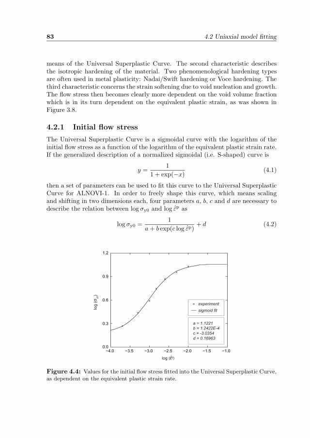
83 4.2 Uniaxial model fitting
means of the Universal Superplastic Curve. The second characteristic describesthe isotropic hardening of the material. Two phenomenological hardening typesare often used in metal plasticity: Nadai/Swift hardening or Voce hardening. Thethird characteristic concerns the strain softening due to void nucleation and growth.The flow stress then becomes clearly more dependent on the void volume fractionwhich is in its turn dependent on the equivalent plastic strain, as was shown inFigure 3.8.
4.2.1 Initial flow stress
The Universal Superplastic Curve is a sigmoidal curve with the logarithm of theinitial flow stress as a function of the logarithm of the equivalent plastic strain rate.If the generalized description of a normalized sigmoidal (i.e. S-shaped) curve is
y =1
1 + exp(−x)(4.1)
then a set of parameters can be used to fit this curve to the Universal SuperplasticCurve for ALNOVI-1. In order to freely shape this curve, which means scalingand shifting in two dimensions each, four parameters a, b, c and d are necessary todescribe the relation between log σy0 and log ˙εp as
log σy0 =1
a + b exp(c log ˙εp)+ d (4.2)
−4.0 −3.5 −3.0 −2.5 −2.0 −1.5 −1.00.0
0.3
0.6
0.9
1.2
experimentsigmoid fitlo
g (
σ y0)
log (εp)
a = 1.1221b = 1.2422E-4c = -3.0354d = 0.16963
Figure 4.4: Values for the initial flow stress fitted into the Universal Superplastic Curve,as dependent on the equivalent plastic strain rate.
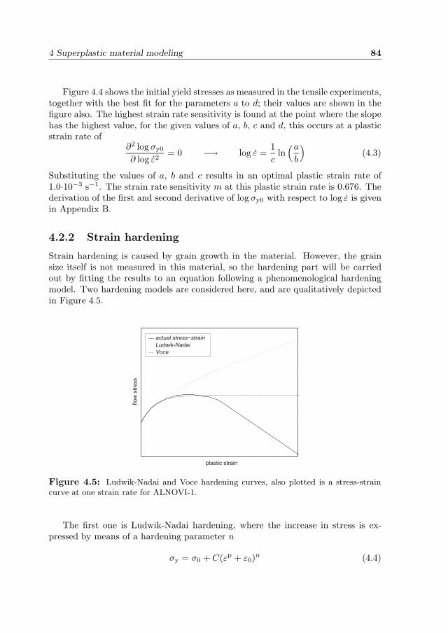
4 Superplastic material modeling 84
Figure 4.4 shows the initial yield stresses as measured in the tensile experiments,together with the best fit for the parameters a to d; their values are shown in thefigure also. The highest strain rate sensitivity is found at the point where the slopehas the highest value, for the given values of a, b, c and d, this occurs at a plasticstrain rate of
∂2 log σy0
∂ log ε2= 0 −→ log ε =
1c
ln(a
b
)(4.3)
Substituting the values of a, b and c results in an optimal plastic strain rate of1.0·10−3 s−1. The strain rate sensitivity m at this plastic strain rate is 0.676. Thederivation of the first and second derivative of log σy0 with respect to log ε is givenin Appendix B.
4.2.2 Strain hardening
Strain hardening is caused by grain growth in the material. However, the grainsize itself is not measured in this material, so the hardening part will be carriedout by fitting the results to an equation following a phenomenological hardeningmodel. Two hardening models are considered here, and are qualitatively depictedin Figure 4.5.
actual stress−strainLudwik-NadaiVoce
plastic strain
flo
w s
tre
ss
Figure 4.5: Ludwik-Nadai and Voce hardening curves, also plotted is a stress-straincurve at one strain rate for ALNOVI-1.
The first one is Ludwik-Nadai hardening, where the increase in stress is ex-pressed by means of a hardening parameter n
σy = σ0 + C(εp + ε0)n (4.4)
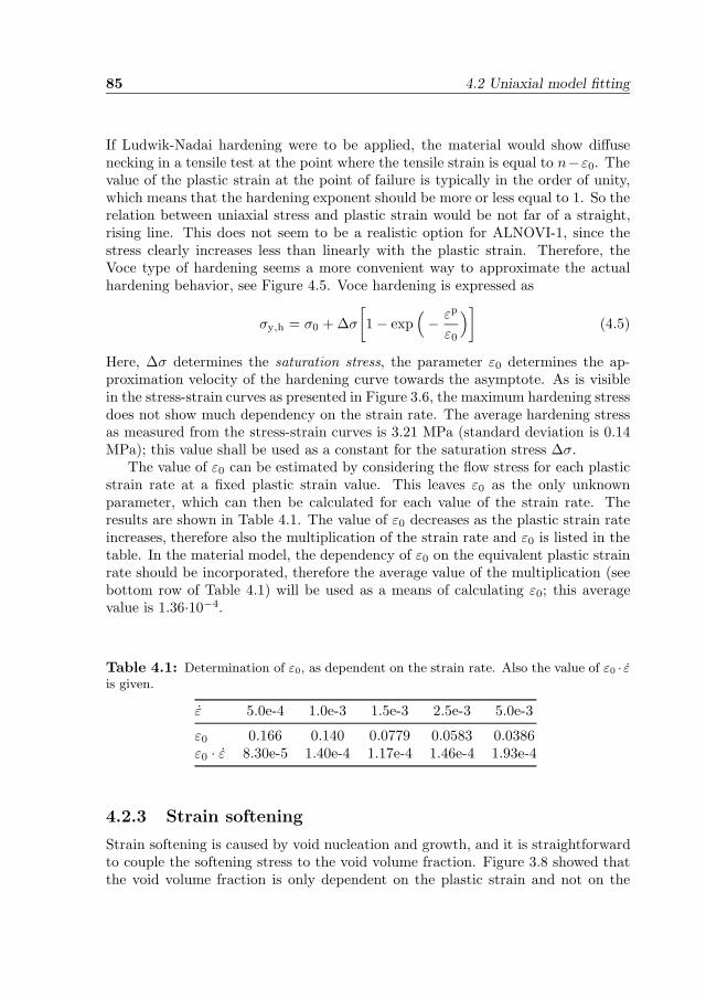
85 4.2 Uniaxial model fitting
If Ludwik-Nadai hardening were to be applied, the material would show diffusenecking in a tensile test at the point where the tensile strain is equal to n−ε0. Thevalue of the plastic strain at the point of failure is typically in the order of unity,which means that the hardening exponent should be more or less equal to 1. So therelation between uniaxial stress and plastic strain would be not far of a straight,rising line. This does not seem to be a realistic option for ALNOVI-1, since thestress clearly increases less than linearly with the plastic strain. Therefore, theVoce type of hardening seems a more convenient way to approximate the actualhardening behavior, see Figure 4.5. Voce hardening is expressed as
σy,h = σ0 + Δσ
[1 − exp
(− εp
ε0
)](4.5)
Here, Δσ determines the saturation stress, the parameter ε0 determines the ap-proximation velocity of the hardening curve towards the asymptote. As is visiblein the stress-strain curves as presented in Figure 3.6, the maximum hardening stressdoes not show much dependency on the strain rate. The average hardening stressas measured from the stress-strain curves is 3.21 MPa (standard deviation is 0.14MPa); this value shall be used as a constant for the saturation stress Δσ.
The value of ε0 can be estimated by considering the flow stress for each plasticstrain rate at a fixed plastic strain value. This leaves ε0 as the only unknownparameter, which can then be calculated for each value of the strain rate. Theresults are shown in Table 4.1. The value of ε0 decreases as the plastic strain rateincreases, therefore also the multiplication of the strain rate and ε0 is listed in thetable. In the material model, the dependency of ε0 on the equivalent plastic strainrate should be incorporated, therefore the average value of the multiplication (seebottom row of Table 4.1) will be used as a means of calculating ε0; this averagevalue is 1.36·10−4.
Table 4.1: Determination of ε0, as dependent on the strain rate. Also the value of ε0 · εis given.
ε 5.0e-4 1.0e-3 1.5e-3 2.5e-3 5.0e-3
ε0 0.166 0.140 0.0779 0.0583 0.0386ε0 · ε 8.30e-5 1.40e-4 1.17e-4 1.46e-4 1.93e-4
4.2.3 Strain softening
Strain softening is caused by void nucleation and growth, and it is straightforwardto couple the softening stress to the void volume fraction. Figure 3.8 showed thatthe void volume fraction is only dependent on the plastic strain and not on the
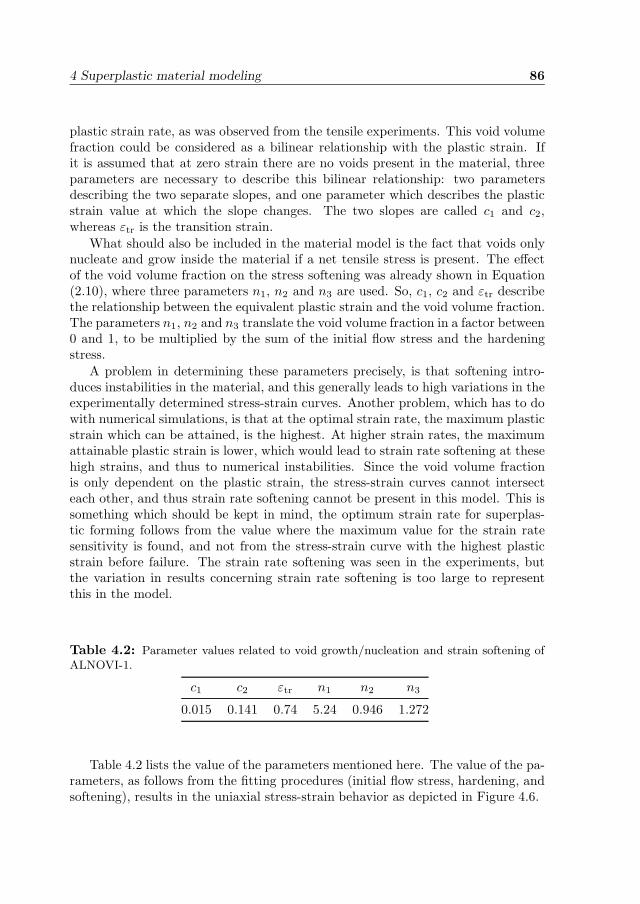
4 Superplastic material modeling 86
plastic strain rate, as was observed from the tensile experiments. This void volumefraction could be considered as a bilinear relationship with the plastic strain. Ifit is assumed that at zero strain there are no voids present in the material, threeparameters are necessary to describe this bilinear relationship: two parametersdescribing the two separate slopes, and one parameter which describes the plasticstrain value at which the slope changes. The two slopes are called c1 and c2,whereas εtr is the transition strain.
What should also be included in the material model is the fact that voids onlynucleate and grow inside the material if a net tensile stress is present. The effectof the void volume fraction on the stress softening was already shown in Equation(2.10), where three parameters n1, n2 and n3 are used. So, c1, c2 and εtr describethe relationship between the equivalent plastic strain and the void volume fraction.The parameters n1, n2 and n3 translate the void volume fraction in a factor between0 and 1, to be multiplied by the sum of the initial flow stress and the hardeningstress.
A problem in determining these parameters precisely, is that softening intro-duces instabilities in the material, and this generally leads to high variations in theexperimentally determined stress-strain curves. Another problem, which has to dowith numerical simulations, is that at the optimal strain rate, the maximum plasticstrain which can be attained, is the highest. At higher strain rates, the maximumattainable plastic strain is lower, which would lead to strain rate softening at thesehigh strains, and thus to numerical instabilities. Since the void volume fractionis only dependent on the plastic strain, the stress-strain curves cannot intersecteach other, and thus strain rate softening cannot be present in this model. This issomething which should be kept in mind, the optimum strain rate for superplas-tic forming follows from the value where the maximum value for the strain ratesensitivity is found, and not from the stress-strain curve with the highest plasticstrain before failure. The strain rate softening was seen in the experiments, butthe variation in results concerning strain rate softening is too large to representthis in the model.
Table 4.2: Parameter values related to void growth/nucleation and strain softening ofALNOVI-1.
c1 c2 εtr n1 n2 n3
0.015 0.141 0.74 5.24 0.946 1.272
Table 4.2 lists the value of the parameters mentioned here. The value of the pa-rameters, as follows from the fitting procedures (initial flow stress, hardening, andsoftening), results in the uniaxial stress-strain behavior as depicted in Figure 4.6.
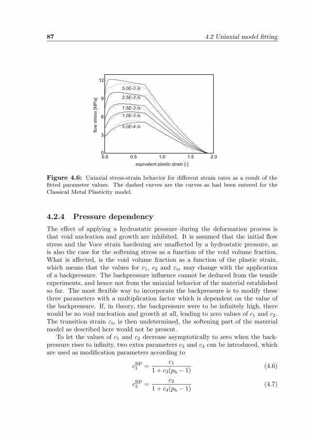
87 4.2 Uniaxial model fitting
0.0 0.5 1.0 1.5 2.0 0
3
6
9
12
equivalent plastic strain [-]
flo
w s
tre
ss [
MP
a]
5.0E-4 /s
1.0E-3 /s1.5E-3 /s
2.5E-3 /s
5.0E-3 /s
Figure 4.6: Uniaxial stress-strain behavior for different strain rates as a result of thefitted parameter values. The dashed curves are the curves as had been entered for theClassical Metal Plasticity model.
4.2.4 Pressure dependency
The effect of applying a hydrostatic pressure during the deformation process isthat void nucleation and growth are inhibited. It is assumed that the initial flowstress and the Voce strain hardening are unaffected by a hydrostatic pressure, asis also the case for the softening stress as a function of the void volume fraction.What is affected, is the void volume fraction as a function of the plastic strain,which means that the values for c1, c2 and εtr may change with the applicationof a backpressure. The backpressure influence cannot be deduced from the tensileexperiments, and hence not from the uniaxial behavior of the material establishedso far. The most flexible way to incorporate the backpressure is to modify thesethree parameters with a multiplication factor which is dependent on the value ofthe backpressure. If, in theory, the backpressure were to be infinitely high, therewould be no void nucleation and growth at all, leading to zero values of c1 and c2.The transition strain εtr is then undetermined, the softening part of the materialmodel as described here would not be present.
To let the values of c1 and c2 decrease asymptotically to zero when the back-pressure rises to infinity, two extra parameters c3 and c4 can be introduced, whichare used as modification parameters according to
cBP1 =
c1
1 + c3(ph − 1)(4.6)
cBP2 =
c2
1 + c4(ph − 1)(4.7)
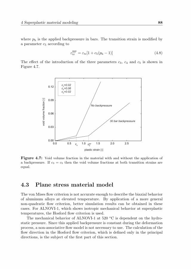
4 Superplastic material modeling 88
where ph is the applied backpressure in bars. The transition strain is modified bya parameter c5 according to
εBPtr = εtr[1 + c5(ph − 1)] (4.8)
The effect of the introduction of the three parameters c3, c4 and c5 is shown inFigure 4.7.
0.0 0.5 1.0 1.5 2.0 2.50.00
0.03
0.06
0.09
0.12
No backpressure
30 bar backpressure
plastic strain [-]
vo
id v
olu
me
fra
ctio
n [
-]
c3=0.02c4=0.06c5=0.02
εtr ε
trBP
Figure 4.7: Void volume fraction in the material with and without the application ofa backpressure. If c3 = c5 then the void volume fractions at both transition strains areequal.
4.3 Plane stress material model
The von Mises flow criterion is not accurate enough to describe the biaxial behaviorof aluminum alloys at elevated temperature. By application of a more generalnon-quadratic flow criterion, better simulation results can be obtained in thesecases. For ALNOVI-1, which shows isotropic mechanical behavior at superplastictemperatures, the Hosford flow criterion is used.
The mechanical behavior of ALNOVI-1 at 520 oC is dependent on the hydro-static pressure. Since this applied backpressure is constant during the deformationprocess, a non-associative flow model is not necessary to use. The calculation of theflow direction in the Hosford flow criterion, which is defined only in the principaldirections, is the subject of the first part of this section.
89 4.3 Plane stress material model
The void volume fraction was made dependent on the equivalent plastic strainas measured from the tensile experiments. In these tests the equivalent plasticstrain was the same as the plastic strain in the tensile direction. In a biaxialstress/strain state, this relation will generally not be true, e.g. if the stress stateis becoming more compressive, the void volume fraction will not increase, but theequivalent plastic strain does increase. The void volume fraction description in abiaxial stress/strain state is the subject of the second part of this section.
4.3.1 Flow directions
Since the Hosford flow criterion is described only in the principal stress directions,see Equation (2.22), it is not possible to derive the updated flow direction from theglobal xyz coordinates directly. Instead of rotating the global stress situation atthe beginning of a time increment and rotating back to an updated angle (whichmeans an extra variable) the stress invariants can be used to determine the flowdirection. The first and second invariants I1 and I2 of a stress vector in the caseof a plane stress situation are
I1 = σxx + σyy = σ1 + σ2 (4.9)
I2 = σxxσyy − σ2xy = σ1σ2 (4.10)
So, σ1 and σ2 can be written in terms of the stress invariants as
σi =I1 ±√
I21 − 4I2
2i = 1, 2 (4.11)
The flow direction ∂φ/∂σ can be written as
∂φ
∂σ=
∂φ
∂σ1
(∂σ1
∂I1
∂I1
∂σ+
∂σ1
∂I2
∂I2
∂σ
)+
∂φ
∂σ2
(∂σ2
∂I1
∂I1
∂σ+
∂σ2
∂I2
∂I2
∂σ
)(4.12)
where ∂φ/∂σi can be derived from the Hosford flow criterion, this is
∂φ
∂σi=
1
(R + 1)σ(n−1)eq
[σ
(n−1)i ± R(σ1 − σ2)(n−1)
]i = 1, 2 (4.13)
in which σeq is the equivalent stress. Further,
∂σi
∂Ii=
⎡⎢⎣
12 (1 + I1
2√
I21−4I2
) −1√I21−4I2
12 (1 − I1
2√
I21−4I2
) 1√I21−4I2
⎤⎥⎦ i = 1, 2 (4.14)
To complete the terms in the equation for ∂φ/∂σ:
∂I1
∂σ=[1 00 1
](4.15)
∂I2
∂σ=[
σyy −2σxy
−2σxy σxx
](4.16)
4 Superplastic material modeling 90
4.3.2 Biaxial-dependent void volume fractions
The values of the parameters c1 and c2, which represent the slopes in the bilinearrelationship between the void volume fraction and the equivalent plastic strain, aredetermined from the tensile (uniaxial) experiments. If the same equivalent plasticstrain is present, but now as a result from a compressive test, then it is obviousthat no voids would nucleate or grow inside the material. Void nucleation andgrowth (and eventually coalescence) is a reaction to tensile stresses or strains. Incompression, the parameters c1 and c2 are zero, or even negative. A negative valuemeans that already existing voids in the material, caused by earlier tension, maybe closed again.
Using the strain tensor Instead of using the equivalent plastic strain for thevoid volume fraction relationship, it may be better to take the plastic strain tensoras a whole into account to determine the change in void volume fraction. Therelationship to describe ξ would then look like
ξ = c∗i · (εpl : I) i = 1, 2 (4.17)
Below the transition strain εtr, this constant is called c∗1, above this strain it isc∗2. This constant can be calculated from the uniaxial strain state. In the uniaxialcase, εpl
xx is equal to the equivalent plastic strain and εplyy = −(1/(R+1)) ·εpl
xx. Thismeans that
ci = c∗1,2(1 − 1R + 1
) i = 1, 2 (4.18)
Soc∗i =
R + 1R
ci i = 1, 2 (4.19)
The transition strain was also defined in terms of the equivalent plastic strain, butin this case it is less obvious than for c1 and c2 that this strain is influenced byplastic strain tensor values. This parameter will therefore be held constant in theuser-defined material model.
Using the stress tensor The stress tensor can be used as an alternative in thedescription of the biaxial-dependent void volume fraction. One advantage of usingthe method of the stress tensor is because the stress is zero in the transverse direc-tion in a uniaxial stress/strain situation. The values of c1 and c2 are not modifiedin this stress situation, and the values of these parameters can be dependent onthe angle ζ as depicted in Figure 4.8. The effective values c∗1 and c∗2 are largerthan c1 and c2 if the second principal stress is positive, and become smaller if thesecond principal stress is negative. These effective values are determined by twoextra parameters x1 and x2. In Table 3.5, a void volume fraction of 1.3 % has beenreported at an equivalent plastic strain of 0.67. This means that in an equibiaxial
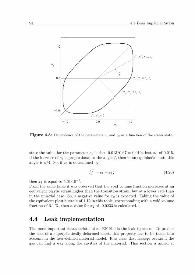
91 4.4 Leak implementation
−1.0 0.0 1.0
−1.0
0.0
1.0
σ1
σ2
c*1, c*
2 = c
1, c
2
c*1, c*
2 > c
1, c
2
ζ
c*1, c*
2 < c
1, c
2
c*1, c*
2 < 0
Figure 4.8: Dependence of the parameters c1 and c2 as a function of the stress state.
state the value for the parameter c1 is then 0.013/0.67 = 0.0194 instead of 0.015.If the increase of c1 is proportional to the angle ζ, then in an equibiaxial state thisangle is π/4. So, if x1 is determined by
c(ζ)1 = c1 + x1ζ (4.20)
then x1 is equal to 5.61·10−3.From the same table it was observed that the void volume fraction increases at anequivalent plastic strain higher than the transition strain, but at a lower rate thanin the uniaxial case. So, a negative value for x2 is expected. Taking the value ofthe equivalent plastic strain of 1.12 in this table, corresponding with a void volumefraction of 6.1 %, then a value for x2 of -0.0233 is calculated.
4.4 Leak implementation
The most important characteristic of an RF Foil is the leak tightness. To predictthe leak of a superplastically deformed sheet, this property has to be taken intoaccount in the user-defined material model. It is clear that leakage occurs if thegas can find a way along the cavities of the material. This section is aimed at
4 Superplastic material modeling 92
finding a relationship between the leak and the void volume fraction. The voidvolume fraction is determined by the plastic strain vector only, which would makeit possible to couple the leak directly to the plastic strain in the material.
4.4.1 Leak prediction
Gases can transport through a sheet or membrane by two phenomena: gas diffusionand gas flow. If the diameter of the channels through which the gas travels issmaller than the mean free path [79] of the gas molecules, then diffusion is themain transport possibility. In general, the mean free path is about 100 nm atatmospheric pressure. If voids are responsible for the gas leak of the RF Foil, thendiffusion is not the main cause in case of gas leak. So, it is assumed here that incase of a gas leak, the gas flows through a channel which is provided by coalescenceof the voids. The gas flow through a channel is dependent on the radius and lengthof the channel, and the pressure difference between both ends [88]:
Q =πd4
cΔp
8ηl(4.21)
where Q is the flow (leak) rate, dc is the diameter of the channel, Δp is the pressuredifference, η is the dynamic viscosity of the gas and l is the length of the channel.The diameter of the channel (or the summation of all channels through the sheet)is related to the void volume fraction. The channel length is related to the resultingsheet thickness. This means that both result types, void volume fraction and sheetthickness, are responsible for the value of the leak rate.
Relating the leak to the void volume fraction has one disadvantage: the voidvolume fraction measurements on the formed bulges show a high variance. Thismay make the leak prediction not accurate enough, but two options are possible.One option is to describe the leak on the safe side of the void volume fraction,the other is to use the mean value of the void volume fraction. The risk is that aformed RF Foil may show a leak value which is too high, but since the amount ofproducts needed is very small, the only risk is that the sheet has to be pressed asecond time, or even maybe a third time. Or, in general: the permitted percentageof scrap products is higher if the production series is smaller. It is also possibleto couple the leak to the plastic strain, but the downside of this method is that adependence on the applied backpressure is also necessary. Since the void volumefraction is less at the same plastic strain at a higher value for the backpressure, it isassumed that the leak value description as a function of this void volume fractionis independent of the backpressure.
The gas flow equation (4.25) is valid for straight channels. It is, however, notto be assumed that the flow channels through the sheet are straight. A number ofcurves and corners will occur, which will be dependent on the channel length andthus on the sheet thickness. Each curve or corner means an extra pressure dropinside the channel because flow energy is lost when the gas flow bends.
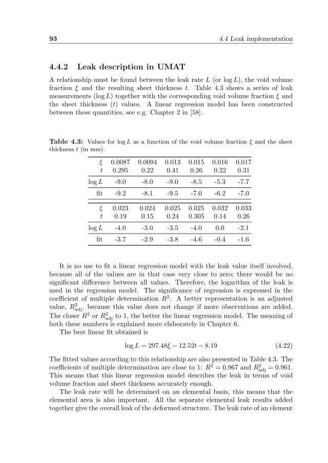
93 4.4 Leak implementation
4.4.2 Leak description in UMAT
A relationship must be found between the leak rate L (or log L), the void volumefraction ξ and the resulting sheet thickness t. Table 4.3 shows a series of leakmeasurements (log L) together with the corresponding void volume fraction ξ andthe sheet thickness (t) values. A linear regression model has been constructedbetween these quantities, see e.g. Chapter 2 in [58].
Table 4.3: Values for log L as a function of the void volume fraction ξ and the sheetthickness t (in mm).
ξ 0.0087 0.0094 0.013 0.015 0.016 0.017t 0.295 0.22 0.41 0.26 0.22 0.31
log L -9.0 -8.0 -9.0 -8.5 -5.3 -7.7
fit -9.2 -8.1 -9.5 -7.0 -6.2 -7.0
ξ 0.023 0.024 0.025 0.025 0.032 0.033t 0.19 0.15 0.24 0.305 0.14 0.26
log L -4.0 -3.0 -3.5 -4.0 0.0 -2.1
fit -3.7 -2.9 -3.8 -4.6 -0.4 -1.6
It is no use to fit a linear regression model with the leak value itself involved,because all of the values are in that case very close to zero; there would be nosignificant difference between all values. Therefore, the logarithm of the leak isused in the regression model. The significance of regression is expressed in thecoefficient of multiple determination R2. A better representation is an adjustedvalue, R2
adj, because this value does not change if more observations are added.The closer R2 or R2
adj to 1, the better the linear regression model. The meaning ofboth these numbers is explained more elaborately in Chapter 6.
The best linear fit obtained is
log L = 297.48ξ − 12.52t− 8.19 (4.22)
The fitted values according to this relationship are also presented in Table 4.3. Thecoefficients of multiple determination are close to 1: R2 = 0.967 and R2
adj = 0.961.This means that this linear regression model describes the leak in terms of voidvolume fraction and sheet thickness accurately enough.
The leak rate will be determined on an elemental basis, this means that theelemental area is also important. All the separate elemental leak results addedtogether give the overall leak of the deformed structure. The leak rate of an element

4 Superplastic material modeling 94
is determined by multiplying the leak rate found as given in Equation (4.22) by theelemental area and dividing by a reference area Aref . The value of this referencearea will be determined in Chapter 5.
4.5 UMAT procedure
This section describes the sequence of steps to be taken to determine the stresssituation and the state variable values in the superplastic alloy ALNOVI-1 for agiven strain increment, during superplastic forming. This is an implicit algorithm.The material shows a high strain rate sensitivity, so the time increment has tobe taken into account within the sequence of steps. A full constitutive model ofALNOVI-1 should strictly speaking also contain a temperature dependency, butsince this is not considered a variable in the forming process, the temperature willnot be included. The model is valid for a temperature of 520 oC, i.e. the optimaltemperature for superplastic forming of ALNOVI-1. The applied backpressureduring forming is an input state variable. The output state variables to be storedare:
• the elastic strain vector εe (3 scalar values), as resulting from Equation (2.28),to be calculated after the stress update procedure has been finished;
• the plastic strain vector εp (3 scalar values), which is the difference betweenthe total strain increment and the elastic strain increment;
• the equivalent plastic strain εp, this is the equivalent plastic strain from theprevious increment plus the value of the plastic multiplier Δλ as resultingfrom the stress update procedure in the current increment;
• the equivalent plastic strain rate ˙εp, which is equal to Δλ/Δt;
• the void volume fraction ξ, calculated from the transition strain εtr, the slopesc1 and c2 and using Equation (4.20);
• the flow stress σf , as a result of Equations (4.2), (4.5) and (2.10).
Below, the steps taken within the user-defined material model description are de-scribed, including the part representing the stress return mapping algorithm.
1. Read all results from the previous increment, these are the stress σ0 and theoutput state variables.
2. Read the strain increment Δε, the time increment Δt and the input statevariable ph, which is the backpressure.
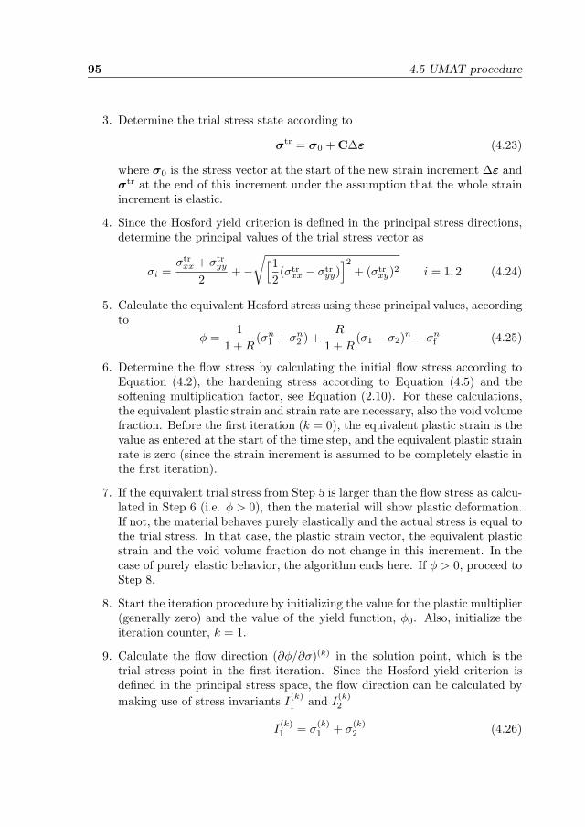
95 4.5 UMAT procedure
3. Determine the trial stress state according to
σtr = σ0 + CΔε (4.23)
where σ0 is the stress vector at the start of the new strain increment Δε andσtr at the end of this increment under the assumption that the whole strainincrement is elastic.
4. Since the Hosford yield criterion is defined in the principal stress directions,determine the principal values of the trial stress vector as
σi =σtr
xx + σtryy
2+ −√[1
2(σtr
xx − σtryy)]2
+ (σtrxy)2 i = 1, 2 (4.24)
5. Calculate the equivalent Hosford stress using these principal values, accordingto
φ =1
1 + R(σn
1 + σn2 ) +
R
1 + R(σ1 − σ2)n − σn
f (4.25)
6. Determine the flow stress by calculating the initial flow stress according toEquation (4.2), the hardening stress according to Equation (4.5) and thesoftening multiplication factor, see Equation (2.10). For these calculations,the equivalent plastic strain and strain rate are necessary, also the void volumefraction. Before the first iteration (k = 0), the equivalent plastic strain is thevalue as entered at the start of the time step, and the equivalent plastic strainrate is zero (since the strain increment is assumed to be completely elastic inthe first iteration).
7. If the equivalent trial stress from Step 5 is larger than the flow stress as calcu-lated in Step 6 (i.e. φ > 0), then the material will show plastic deformation.If not, the material behaves purely elastically and the actual stress is equal tothe trial stress. In that case, the plastic strain vector, the equivalent plasticstrain and the void volume fraction do not change in this increment. In thecase of purely elastic behavior, the algorithm ends here. If φ > 0, proceed toStep 8.
8. Start the iteration procedure by initializing the value for the plastic multiplier(generally zero) and the value of the yield function, φ0. Also, initialize theiteration counter, k = 1.
9. Calculate the flow direction (∂φ/∂σ)(k) in the solution point, which is thetrial stress point in the first iteration. Since the Hosford yield criterion isdefined in the principal stress space, the flow direction can be calculated bymaking use of stress invariants I
(k)1 and I
(k)2
I(k)1 = σ
(k)1 + σ
(k)2 (4.26)

4 Superplastic material modeling 96
I(k)2 = σ
(k)1 σ
(k)2 (4.27)
Then (omitting the superscript k)
∂φ
∂σ=
∂φ
∂σ1
(∂σ1
∂I1· ∂I1
∂σ+
∂σ1
∂I2· ∂I2
∂σ
)+
∂φ
∂σ2
(∂σ2
∂I1· ∂I1
∂σ+
∂σ2
∂I2· ∂I2
∂σ
)(4.28)
10. Calculate the derivative of the flow direction, ∂2φ/∂σ2. The best method asa compromise between calculation speed and accuracy is to determine thissecond order matrix numerically instead of analytically.
11. Determine the flow stress with an equivalent plastic strain input equal tothe plastic multiplier Δλ(k) and an equivalent plastic strain rate equal toΔλ(k)/Δt. The use of the plastic multiplier as equivalent plastic strain is onlypermitted if the Hosford yield criterion is written such that ∂φ/∂σf = −1, asin
φ =[ 11 + R
(σn1 + σn
2 ) +R
1 + R(σ1 − σ2)n
]1/n
− σf (4.29)
12. Two equations have to be solved simultaneously, the first one concerns thefact that the total strain increment in each step is an addition of an elasticstrain increment and a plastic strain increment. Written in a residual format,this reads
rσ = Δε − Δεel − Δεpl = 0 (4.30)
The second equation states that the value of the flow function in case ofplastic deformation is equal to zero:
rφ = φ = 0 (4.31)
Rewriting the first equation gives
rσ = Δε − C−1Δσ − Δλ∂φ
∂σ= 0 (4.32)
To solve these equations in a Newton iteration scheme, they have to be lin-earized. For both equations, this results in case of the k-th iteration:
rσ(k) =
(C−1 + Δλ
∂2φ
∂σ2
)(k)
dσ(k) + dλ(k)( ∂φ
∂σ
)(k)
(4.33)
rφ(k) =
( ∂φ
∂σ
)(k)
dσ(k) −( ∂φ
∂εp
)(k)
dλ(k) (4.34)
Rewrite this set of equations as
C−1 · Δ(sol) = r (4.35)
97 4.6 Summary and conclusions
in which
C−1 =
⎡⎣[C−1 + Δλ ∂2φ
∂σ2 ] { ∂φ∂σ}
{ ∂φ∂σ}T − ∂φ
∂εp
⎤⎦
(k)
(4.36)
Δ(sol) ={{Δσ}(k+1) Δλ(k+1)
}T(4.37)
r ={{Δε − C−1 · σ − Δλ ∂φ
∂σ}(k) φ(k)}T
(4.38)
Iterate until φ has reached a value which is smaller than a predefined tolerancevalue. The final solution for Δ(sol) has then been found.
13. Update the stress vector, the state variables and the iteration counter. Thesubincremental procedure is invoked if Δ(sol) is multiplied by a factor be-tween 0 and 1 before the stress and equivalent plastic strain are updated.This factor can be applied during the whole iteration process, or only duringthe first iterations. Also, this factor does not have to be the same for alliterations. Go to step 9 if the solution has not been converged, or else go tostep 14.
14. Store the stress and the state variables.
4.6 Summary and conclusions
This chapter presented the necessity of developing a user-defined material modelin favor of the standard material models which are incorporated in ABAQUS. TheDrucker-Prager model and Gurson’s model have too many limitations to be usefulas a constitutive model base for superplasticity. The standard Classical MetalPlasticity model with strain-rate dependency seemed the best option. However, athigher values for the equivalent plastic strain, the results were not accurate enoughin case of simulation of the bulge experiment. Therefore a user-defined materialmodel had to be developed.
This user-defined material model consists of 12 material parameters to describethe uniaxial behavior of ALNOVI-1. These parameters are used to define the initialflow stress, a hardening stress and a softening factor between 0 and 1 to accountfor the effect of the void volume fraction. Three extra parameters are necessary toaccount for the effect of the application of a backpressure during the deformationprocess. It is important that these three parameters are used in the case that thebackpressure does not change during the deformation process, which is generallythe case in superplastic forming processes.
The Hosford yield criterion has been applied with n = 8, this criterion is de-fined in the principal stress directions only. To account for this situation, the flowdirection can be determined by using the stress invariants. This avoids the need torotate the stress vector about an angle which has to be determined in the iteration

4 Superplastic material modeling 98
process. The first derivative of the flow function can be derived analytically, thesecond derivative is determined numerically in the user-defined material model.
The void volume fraction was determined as dependent on the equivalent plas-tic strain in a uniaxial stress situation. Two extra parameters were necessary todetermine the void volume fraction in the case of a stress situation outside theuniaxial case.
The leak rate was found to be dependent on the void volume fraction and theresulting sheet thickness. This is what can be expected if the gas flows through thesheet instead of by a diffusion process. A linear relationship was found which isaccurate enough between the logarithm of the leak rate, the void volume fractionand the sheet thickness.
In the next chapter, verification simulations will be carried out to verify theaccuracy of the material model. All experiment types will be verified: uniaxialexperiments, free bulge experiments and die bulge experiments. The last category,which was not mentioned in this chapter, is used to obtain a more detailed view ofthe friction coefficient between ALNOVI-1 and the die material.
5. Verification of the materialmodel
The material model as established in the previous chapter will be verified by sim-ulating the experiments. Simulations of the tensile tests have to show the abilityof the material model to mimic the experimental force-displacement curves in thecase of a uniaxial stress state. Also the void volume fractions, which were measuredin the strain/vvf tensile tests, will be compared with simulations. In case of toohigh deviations, the values for the parameters should be adjusted, i.e. minimizingthe difference between the corresponding load-displacement curves. Simulation ofthe tensile experiments is the subject of Section 5.1.
Simulations of the free and die bulge experiments are necessary to verify thebiaxial behavior of the material model. Not only the prediction of the deformationstate is important, but also the predicted leak value must be accurate enough.Section 5.2 discusses the simulation results of the free bulge experiments, whereasSection 5.3 is dedicated to the die bulge experiments. The parameters in thematerial model should be adjusted slightly if the simulation results do not match theexperimental results accurately enough. These adjustments should then only coverthe parameters which do not (or hardly) influence the uniaxial material behavior.Also the parameters which deal with the application of a backpressure are checkedwith the biaxial simulations.
5.1 Tensile test simulations
This section describes the results of the finite element simulations concerning thetensile experiments. Firstly, the simulated load-displacement curves are comparedwith the corresponding curves as found in the destructive tensile tests. The resultsmay show that the material parameters describing the uniaxial behavior have to beadjusted. Secondly, the plastic strain rate is checked in the simulations, verifyingthe assumption that this value is constant throughout one test. Thirdly, the voidvolume fractions are calculated and compared with the experimentally found voidvolume fractions, as resulted from the strain/vvf tensile tests.
99
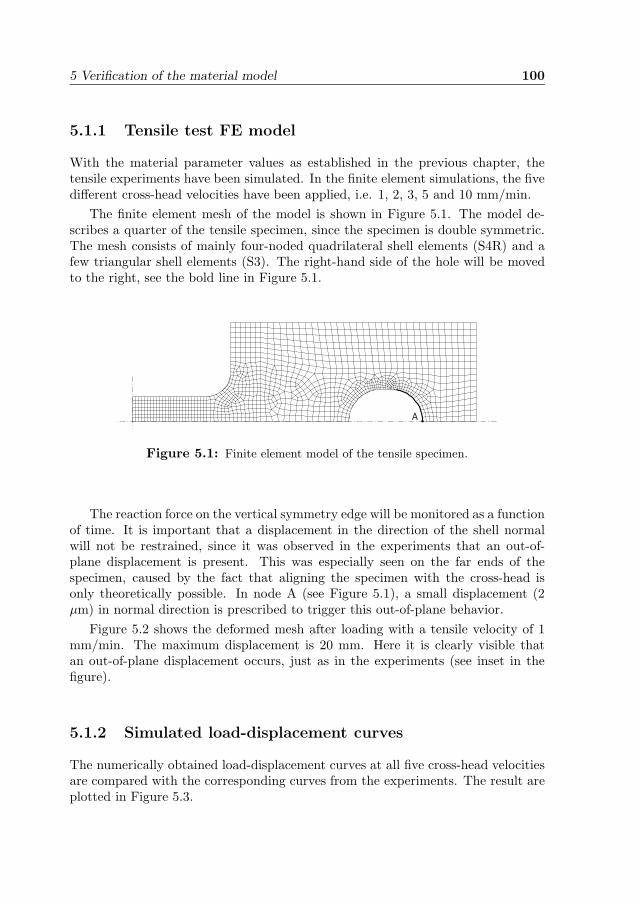
5 Verification of the material model 100
5.1.1 Tensile test FE model
With the material parameter values as established in the previous chapter, thetensile experiments have been simulated. In the finite element simulations, the fivedifferent cross-head velocities have been applied, i.e. 1, 2, 3, 5 and 10 mm/min.
The finite element mesh of the model is shown in Figure 5.1. The model de-scribes a quarter of the tensile specimen, since the specimen is double symmetric.The mesh consists of mainly four-noded quadrilateral shell elements (S4R) and afew triangular shell elements (S3). The right-hand side of the hole will be movedto the right, see the bold line in Figure 5.1.
A
Figure 5.1: Finite element model of the tensile specimen.
The reaction force on the vertical symmetry edge will be monitored as a functionof time. It is important that a displacement in the direction of the shell normalwill not be restrained, since it was observed in the experiments that an out-of-plane displacement is present. This was especially seen on the far ends of thespecimen, caused by the fact that aligning the specimen with the cross-head isonly theoretically possible. In node A (see Figure 5.1), a small displacement (2μm) in normal direction is prescribed to trigger this out-of-plane behavior.
Figure 5.2 shows the deformed mesh after loading with a tensile velocity of 1mm/min. The maximum displacement is 20 mm. Here it is clearly visible thatan out-of-plane displacement occurs, just as in the experiments (see inset in thefigure).
5.1.2 Simulated load-displacement curves
The numerically obtained load-displacement curves at all five cross-head velocitiesare compared with the corresponding curves from the experiments. The result areplotted in Figure 5.3.
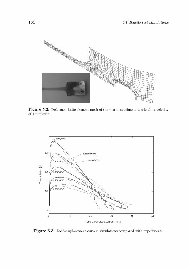
101 5.1 Tensile test simulations
Figure 5.2: Deformed finite element mesh of the tensile specimen, at a loading velocityof 1 mm/min.
0 10 20 30 40 50
0
10
20
30
1 mm/min
5 mm/min
2 mm/min
3 mm/min
10 mm/min
experiment
simulation
Tensile bar displacement [mm]
Tensile
forc
e [N
]
Figure 5.3: Load-displacement curves: simulations compared with experiments.
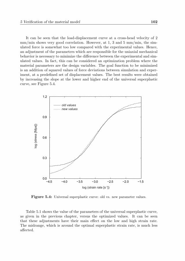
5 Verification of the material model 102
It can be seen that the load-displacement curve at a cross-head velocity of 2mm/min shows very good correlation. However, at 1, 3 and 5 mm/min, the sim-ulated force is somewhat too low compared with the experimental values. Hence,an adjustment of the parameters which are responsible for the uniaxial mechanicalbehavior is necessary to minimize the difference between the experimental and sim-ulated values. In fact, this can be considered an optimization problem where thematerial parameters are the design variables. The goal function to be minimizedis an addition of squared values of force deviations between simulation and exper-iment, at a predefined set of displacement values. The best results were obtainedby increasing the slope at the lower and higher end of the universal superplasticcurve, see Figure 5.4.
−4.5 −4.0 −3.5 −3.0 −2.5 −2.0 −1.50.0
0.3
0.6
0.9
1.2
old valuesnew values
log (strain rate [s-1])
log (
str
ess [M
pa])
Figure 5.4: Universal superplastic curve: old vs. new parameter values.
Table 5.1 shows the value of the parameters of the universal superplastic curve,as given in the previous chapter, versus the optimized values. It can be seenthat these adjustments have their main effect on the low and high strain rate.The midrange, which is around the optimal superplastic strain rate, is much lessaffected.
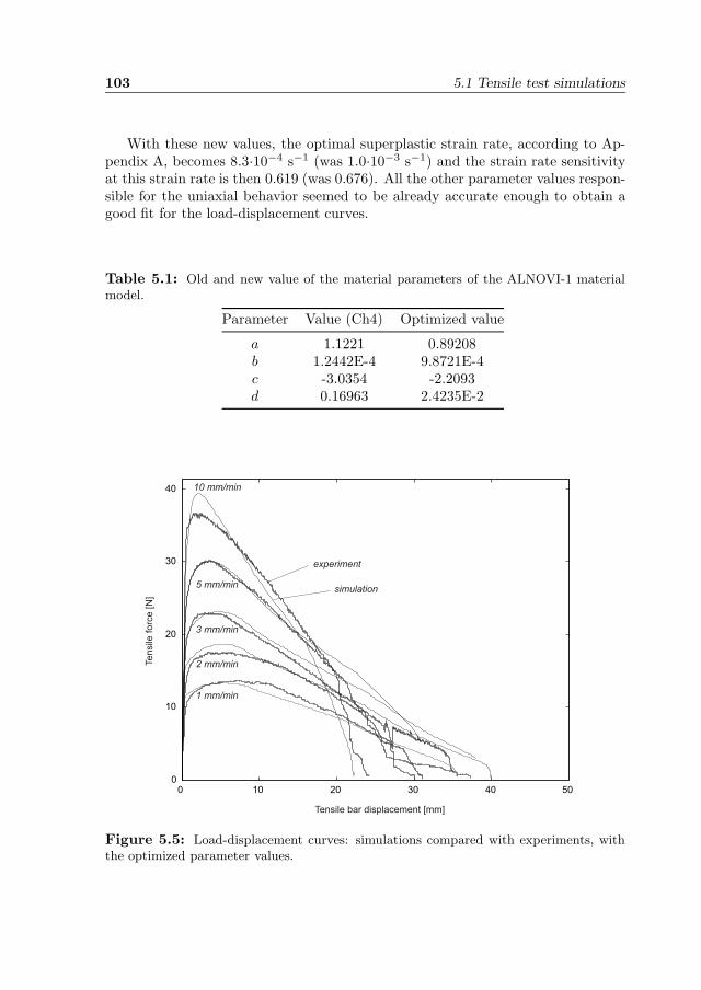
103 5.1 Tensile test simulations
With these new values, the optimal superplastic strain rate, according to Ap-pendix A, becomes 8.3·10−4 s−1 (was 1.0·10−3 s−1) and the strain rate sensitivityat this strain rate is then 0.619 (was 0.676). All the other parameter values respon-sible for the uniaxial behavior seemed to be already accurate enough to obtain agood fit for the load-displacement curves.
Table 5.1: Old and new value of the material parameters of the ALNOVI-1 materialmodel.
Parameter Value (Ch4) Optimized value
a 1.1221 0.89208b 1.2442E-4 9.8721E-4c -3.0354 -2.2093d 0.16963 2.4235E-2
0 10 20 30 40 50 0
10
20
30
40
1 mm/min
5 mm/min
2 mm/min
3 mm/min
10 mm/min
experiment
simulation
Tensile bar displacement [mm]
Tensile
forc
e [N
]
Figure 5.5: Load-displacement curves: simulations compared with experiments, withthe optimized parameter values.

5 Verification of the material model 104
With these optimized values, the tensile experiments have been simulated asecond time, resulting in load-displacement curves which lie on average closer tothe experimental curves. Figure 5.5 shows that at 1, 3 and 5 mm/min, the simulatedcurves are closer to the experimental curves, at a cost of less accuracy at 2 and10 mm/min. Since a velocity of 10 mm/min results in a strain rate which is notdesired in superplastic forming processes, this curve is considered less importantthan the curve at the other velocities.
5.1.3 Simulated strain rates
The void volume fraction is one of the output state variables built into the mate-rial model, and is used to calculate the strain softening. From Figure 3.8 it wasconcluded that the void volume fraction can be considered as dependent only onthe equivalent plastic strain, and not on the strain rate. The results as presentedin Figure 3.6 assumed constant values for the strain rate. From these strain ratevalues and the total loading time, a value for the equivalent plastic strain was cal-culated. The simulations of the tensile experiments have to confirm the assumptionof constant strain rate during the loading process. Results of these simulations areshown in Figure 5.6.
As can be seen from the plots, the plastic strain rates can be considered constantto a great extent, but the loading rate of 10 mm/min is an exception. The dottedlines in the figure show the strain rates as used in Chapter 3, which are very goodin accordance with the simulation results. Only in the case of a loading rate of 10mm/min, the plastic strain rates cannot be considered constant.
5.1.4 Simulated void volume fractions
As was concluded in the previous subsection, the strain rates can be consideredconstant in the tensile experiments, apart from the tests at the highest loadingrate of 10 mm/min. The plastic strain is increasing monotonically with increasingcross-head displacement. The void volume fractions as a function of the cross-head displacement for both simulation and experiment is given in Figure 5.7. Thesimulation results approximate the experimental results with reasonable accuracy.
In this figure, a point is present where the slopes of the curves instantaneouslychange; this is a result of the abrupt change which is coded in the material model.At a strain below the transition strain εtr, the slope is determined by the parameterc1. If the equivalent plastic strain exceeds this transition strain, the slope changesfrom c1 to c2. Figure 5.7 shows that the slopes resulting from the simulations arecorrect, the transition strain seems somewhat too low. However, since the differenceis not too high, the free bulge simulations will be performed with the existing valuefor the transition strain. If the same kind of error is found in these simulations,the transition strain will be adjusted.
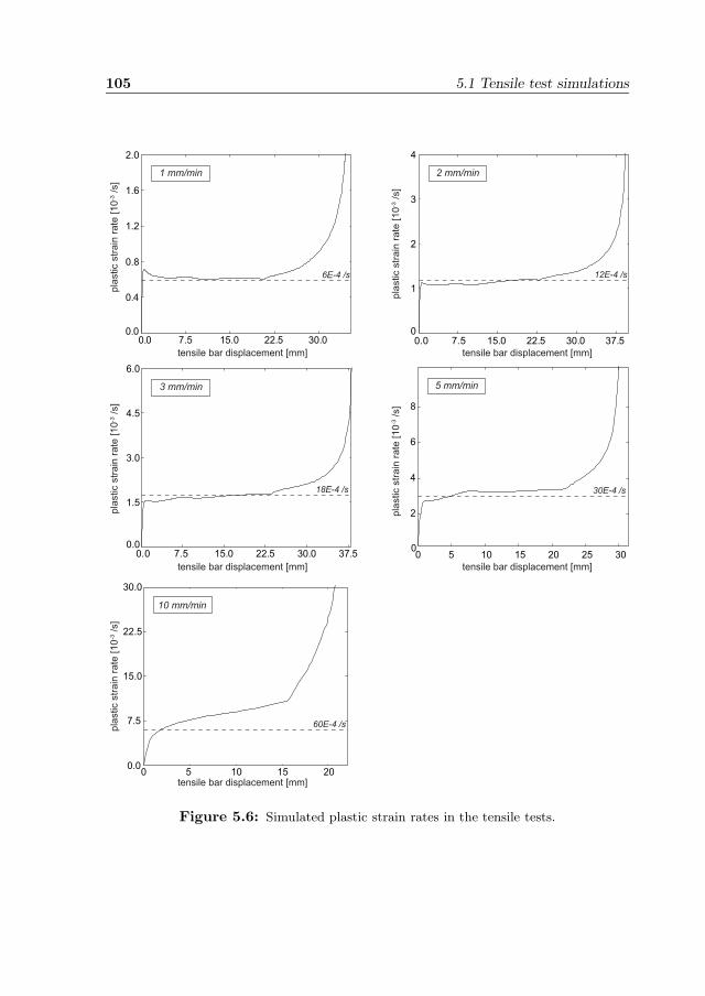
105 5.1 Tensile test simulations
0 5 10 15 20 25 300
2
4
6
8
5 mm/min
tensile bar displacement [mm]
pla
stic s
tra
in r
ate
[1
0-3 /s]
0.0 7.5 15.0 22.5 30.0 37.50.0
1.5
3.0
4.5
6.0
3 mm/min
tensile bar displacement [mm]
pla
stic s
tra
in r
ate
[1
0-3 /s]
0.0 7.5 15.0 22.5 30.0 37.50
1
2
3
4
2 mm/min
tensile bar displacement [mm]
pla
stic s
tra
in r
ate
[1
0-3 /s]
0.0 7.5 15.0 22.5 30.00.0
0.4
0.8
1.2
1.6
2.0
1 mm/min
tensile bar displacement [mm]
pla
stic s
tra
in r
ate
[1
0-3 /s]
0 5 10 15 200.0
7.5
15.0
22.5
30.0
tensile bar displacement [mm]
pla
stic s
tra
in r
ate
[1
0-3 /
s]
6E-4 /s 12E-4 /s
18E-4 /s 30E-4 /s
60E-4 /s
10 mm/min
Figure 5.6: Simulated plastic strain rates in the tensile tests.
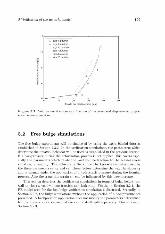
5 Verification of the material model 106
0 10 20 30 40 50 0
4
8
12
16
Tensile bar displacement [mm]
Vo
id V
olu
me
Fra
ctio
n [
%]
exp 1 mm/min
exp 10 mm/minsim 1 mm/minsim 3 mm/minsim 10 mm/min
exp 3 mm/min
Figure 5.7: Void volume fractions as a function of the cross-head displacement, exper-iment versus simulation.
5.2 Free bulge simulations
The free bulge experiments will be simulated by using the extra biaxial data asestablished in Section 4.3.2. In the verification simulations, the parameters whichdetermine the uniaxial behavior will be used as established in the previous section.If a backpressure during the deformation process is not applied, this covers espe-cially the parameters which relate the void volume fraction to the biaxial stresssituation, x1 and x2. The influence of the applied backpressure is determined bythe three parameters c3, c4 and c5. These factors determine the way the slopes c1
and c2 change under the application of a hydrostatic pressure during the formingprocess. Also the transition strain εtr can be influenced by this backpressure.
This section describes the verification simulations in terms of bulge height, topwall thickness, void volume fraction and leak rate. Firstly, in Section 5.2.1, theFE model used for the free bulge verification simulation is discussed. Secondly, inSection 5.2.2, the bulge simulations without the application of a backpressure arepresented. A backpressure application does not modify the parameters determinedhere, so these verification simulations can be dealt with separately. This is done inSection 5.2.3.
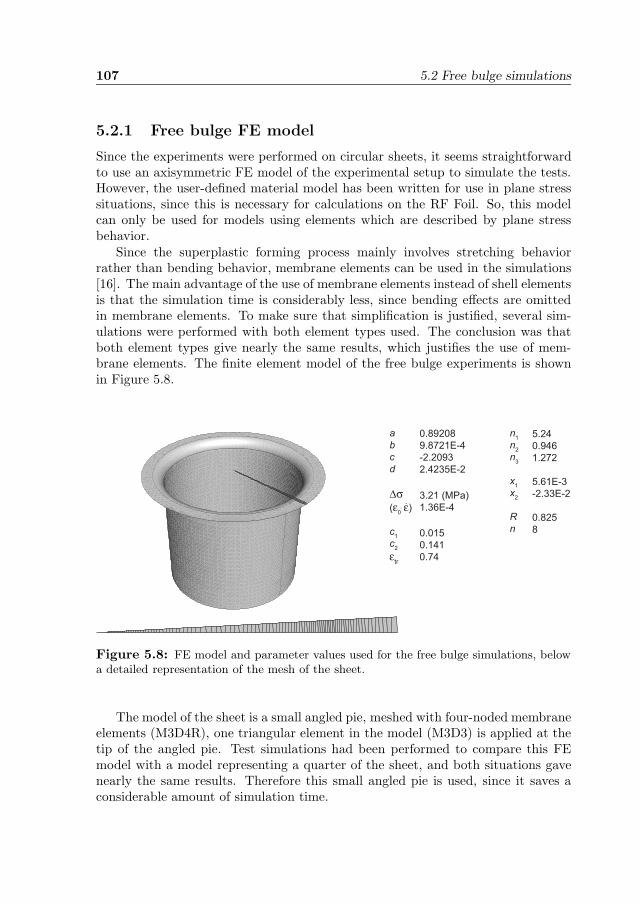
107 5.2 Free bulge simulations
5.2.1 Free bulge FE model
Since the experiments were performed on circular sheets, it seems straightforwardto use an axisymmetric FE model of the experimental setup to simulate the tests.However, the user-defined material model has been written for use in plane stresssituations, since this is necessary for calculations on the RF Foil. So, this modelcan only be used for models using elements which are described by plane stressbehavior.
Since the superplastic forming process mainly involves stretching behaviorrather than bending behavior, membrane elements can be used in the simulations[16]. The main advantage of the use of membrane elements instead of shell elementsis that the simulation time is considerably less, since bending effects are omittedin membrane elements. To make sure that simplification is justified, several sim-ulations were performed with both element types used. The conclusion was thatboth element types give nearly the same results, which justifies the use of mem-brane elements. The finite element model of the free bulge experiments is shownin Figure 5.8.
abcd
Δσ(ε
0 ε)
c1
c2
εtr
0.89208
9.8721E-4
-2.2093
2.4235E-2
3.21 (MPa)
1.36E-4
0.015
0.141
0.74
n1
n2
n3
x1
x2
Rn
5.24
0.946
1.272
5.61E-3
-2.33E-2
0.825
8
Figure 5.8: FE model and parameter values used for the free bulge simulations, belowa detailed representation of the mesh of the sheet.
The model of the sheet is a small angled pie, meshed with four-noded membraneelements (M3D4R), one triangular element in the model (M3D3) is applied at thetip of the angled pie. Test simulations had been performed to compare this FEmodel with a model representing a quarter of the sheet, and both situations gavenearly the same results. Therefore this small angled pie is used, since it saves aconsiderable amount of simulation time.
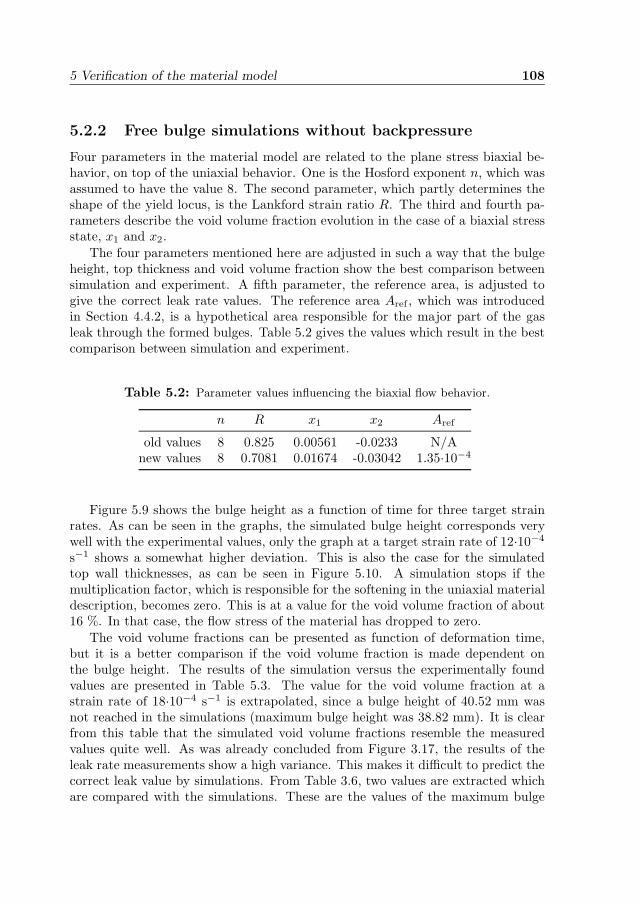
5 Verification of the material model 108
5.2.2 Free bulge simulations without backpressure
Four parameters in the material model are related to the plane stress biaxial be-havior, on top of the uniaxial behavior. One is the Hosford exponent n, which wasassumed to have the value 8. The second parameter, which partly determines theshape of the yield locus, is the Lankford strain ratio R. The third and fourth pa-rameters describe the void volume fraction evolution in the case of a biaxial stressstate, x1 and x2.
The four parameters mentioned here are adjusted in such a way that the bulgeheight, top thickness and void volume fraction show the best comparison betweensimulation and experiment. A fifth parameter, the reference area, is adjusted togive the correct leak rate values. The reference area Aref , which was introducedin Section 4.4.2, is a hypothetical area responsible for the major part of the gasleak through the formed bulges. Table 5.2 gives the values which result in the bestcomparison between simulation and experiment.
Table 5.2: Parameter values influencing the biaxial flow behavior.
n R x1 x2 Aref
old values 8 0.825 0.00561 -0.0233 N/Anew values 8 0.7081 0.01674 -0.03042 1.35·10−4
Figure 5.9 shows the bulge height as a function of time for three target strainrates. As can be seen in the graphs, the simulated bulge height corresponds verywell with the experimental values, only the graph at a target strain rate of 12·10−4
s−1 shows a somewhat higher deviation. This is also the case for the simulatedtop wall thicknesses, as can be seen in Figure 5.10. A simulation stops if themultiplication factor, which is responsible for the softening in the uniaxial materialdescription, becomes zero. This is at a value for the void volume fraction of about16 %. In that case, the flow stress of the material has dropped to zero.
The void volume fractions can be presented as function of deformation time,but it is a better comparison if the void volume fraction is made dependent onthe bulge height. The results of the simulation versus the experimentally foundvalues are presented in Table 5.3. The value for the void volume fraction at astrain rate of 18·10−4 s−1 is extrapolated, since a bulge height of 40.52 mm wasnot reached in the simulations (maximum bulge height was 38.82 mm). It is clearfrom this table that the simulated void volume fractions resemble the measuredvalues quite well. As was already concluded from Figure 3.17, the results of theleak rate measurements show a high variance. This makes it difficult to predict thecorrect leak value by simulations. From Table 3.6, two values are extracted whichare compared with the simulations. These are the values of the maximum bulge
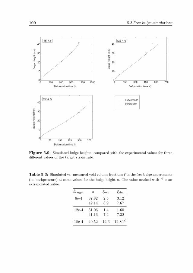
109 5.2 Free bulge simulations
0 300 600 900 1200 1500 0
10
20
30
40
0 150 300 450 600 750 0
10
20
30
40
0 75 150 225 300 375 0
10
20
30
40
Deformation time [s]
Deformation time [s]
Deformation time [s]
Bu
lge
He
igh
t [m
m]
Bu
lge
He
igh
t [m
m]
Bu
lge
He
igh
t [m
m]
18E-4 /s
12E-4 /s6E-4 /s
ExperimentSimulation
Figure 5.9: Simulated bulge heights, compared with the experimental values for threedifferent values of the target strain rate.
Table 5.3: Simulated vs. measured void volume fractions ξ in the free bulge experiments
(no backpressure) at some values for the bulge height u. The value marked with ∗) is anextrapolated value.
˙εtarget u ξexp ξsim
6e-4 37.82 2.5 3.1242.14 8.9 7.67
12e-4 31.06 1.4 1.6041.16 7.2 7.32
18e-4 40.52 12.6 12.89∗)
5 Verification of the material model 110
0 10 20 30 40 500.0
0.2
0.4
0.6
0.8
0 10 20 30 40 500.0
0.2
0.4
0.6
0.8
0 10 20 30 40 500.0
0.2
0.4
0.6
0.8
Bulge Height [mm]
Bulge Height [mm]
Bulge Height [mm]
To
p W
all
Th
ickn
ess [
mm
]
To
p W
all
Th
ickn
ess [
mm
]
To
p W
all
Th
ickn
ess [
mm
]
18E-4 /s
12E-4 /s6E-4 /s
ExperimentSimulation
Figure 5.10: Simulated top wall thicknesses, compared with the experimental valuesfor three different values of the target strain rate.
heights reached at a predefined level of the leak rate, without the application ofa backpressure. For a leak rate of 10−8 mbar l/s and an initial sheet thickness of0.8 mm, this was 31.31 mm; for a leak rate of 100 mbar l/s, this bulge height was37.97 mm.
Table 5.4: Simulated bulge heights (in mm) where the leak rate reaches a value of 10−8
mbar l/s and 100 mbar l/s.
˙εtarget log L = −8 log L = 0
6e-4 32.68 38.4512e-4 31.59 37.2518e-4 31.12 35.13
experiment 31.31 37.97
Table 5.4 shows the corresponding values of the bulge height for the three
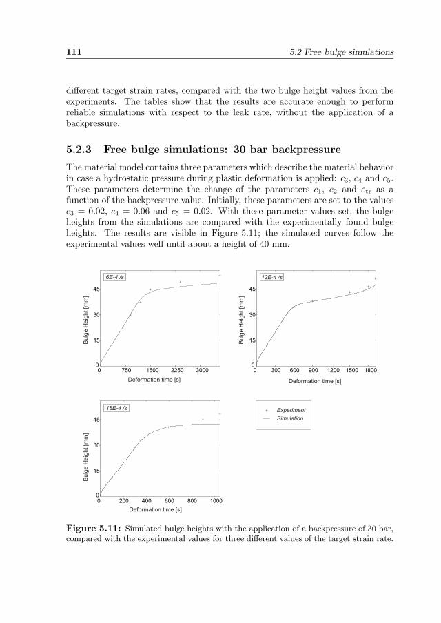
111 5.2 Free bulge simulations
different target strain rates, compared with the two bulge height values from theexperiments. The tables show that the results are accurate enough to performreliable simulations with respect to the leak rate, without the application of abackpressure.
5.2.3 Free bulge simulations: 30 bar backpressure
The material model contains three parameters which describe the material behaviorin case a hydrostatic pressure during plastic deformation is applied: c3, c4 and c5.These parameters determine the change of the parameters c1, c2 and εtr as afunction of the backpressure value. Initially, these parameters are set to the valuesc3 = 0.02, c4 = 0.06 and c5 = 0.02. With these parameter values set, the bulgeheights from the simulations are compared with the experimentally found bulgeheights. The results are visible in Figure 5.11; the simulated curves follow theexperimental values well until about a height of 40 mm.
0 750 1500 2250 3000 0
15
30
45
0 300 600 900 1200 1500 1800 0
15
30
45
0 200 400 600 800 1000 0
15
30
45
Deformation time [s]
Bu
lge
He
igh
t [m
m]
Deformation time [s]
Bu
lge
He
igh
t [m
m]
Deformation time [s]
Bu
lge
He
igh
t [m
m]
18E-4 /s
12E-4 /s6E-4 /s
ExperimentSimulation
Figure 5.11: Simulated bulge heights with the application of a backpressure of 30 bar,compared with the experimental values for three different values of the target strain rate.
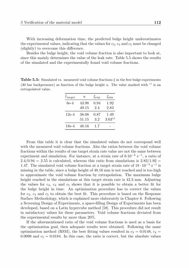
5 Verification of the material model 112
With increasing deformation time, the predicted bulge height underestimatesthe experimental values, indicating that the values for c3, c4 and c5 must be changed(slightly) to overcome this difference.
Besides the bulge height, the void volume fraction is also important to look at,since this mainly determines the value of the leak rate. Table 5.5 shows the resultsof the simulated and the experimentally found void volume fractions.
Table 5.5: Simulated vs. measured void volume fractions ξ in the free bulge experiments
(30 bar backpressure) as function of the bulge height u. The value marked with ∗) is anextrapolated value.
˙εtarget u ξexp ξsim
6e-4 43.98 0.94 1.9249.15 2.4 2.83
12e-4 38.08 0.87 1.4951.15 3.2 3.63∗)
18e-4 48.16 1.7 -
From this table it is clear that the simulated values do not correspond wellwith the measured void volume fractions. Also the ratios between the void volumefractions within the results of one target strain rate value are not the same betweenexperiment and simulation. For instance, at a strain rate of 6·10−4 s−1, a ratio of2.4/0.94 = 2.55 is calculated, whereas this ratio from simulations is 2.83/1.92 =1.47. The simulated void volume fraction at a target strain rate of 18 · 10−4 s−1 ismissing in the table, since a bulge height of 48.16 mm is not reached and is too highto approximate the void volume fraction by extrapolation. The maximum bulgeheight reached in the simulations at this target strain rate is 42.3 mm. Adjustingthe values for c3, c4 and c5 shows that it is possible to obtain a better fit forthe bulge height in time. An optimization procedure has to correct the valuesfor c3, c4 and c5 to obtain the best fit. This procedure is based on the ResponseSurface Methodology, which is explained more elaborately in Chapter 6. Followinga Screening Design of Experiments, a space-filling Design of Experiments has beendeveloped, based on a Latin hypercube method [58]. This procedure did not resultin satisfactory values for these parameters. Void volume fractions deviated fromthe experimental results by more than 20%.
If the aforementioned ratio of the void volume fractions is used as a basis forthe optimization goal, then adequate results were obtained. Following the sameoptimization method (RSM), the best fitting values resulted in c3 = 0.0148, c4 =0.0098 and c5 = 0.0184. In this case, the ratio is correct, but the absolute values
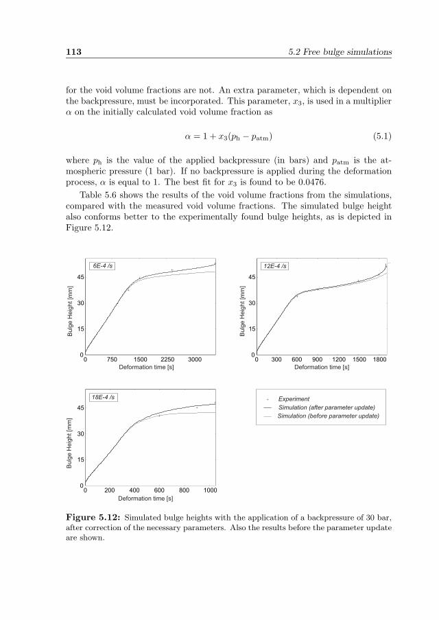
113 5.2 Free bulge simulations
for the void volume fractions are not. An extra parameter, which is dependent onthe backpressure, must be incorporated. This parameter, x3, is used in a multiplierα on the initially calculated void volume fraction as
α = 1 + x3(ph − patm) (5.1)
where ph is the value of the applied backpressure (in bars) and patm is the at-mospheric pressure (1 bar). If no backpressure is applied during the deformationprocess, α is equal to 1. The best fit for x3 is found to be 0.0476.
Table 5.6 shows the results of the void volume fractions from the simulations,compared with the measured void volume fractions. The simulated bulge heightalso conforms better to the experimentally found bulge heights, as is depicted inFigure 5.12.
0 750 1500 2250 3000 0
15
30
45
0 300 600 900 1200 1500 1800 0
15
30
45
0 200 400 600 800 1000 0
15
30
45
Deformation time [s]
Bulg
e H
eig
ht [m
m]
Deformation time [s]
Bulg
e H
eig
ht [m
m]
Deformation time [s]
Bulg
e H
eig
ht [m
m]
18E-4 /s
12E-4 /s6E-4 /s
ExperimentSimulation (after parameter update)Simulation (before parameter update)
Figure 5.12: Simulated bulge heights with the application of a backpressure of 30 bar,after correction of the necessary parameters. Also the results before the parameter updateare shown.
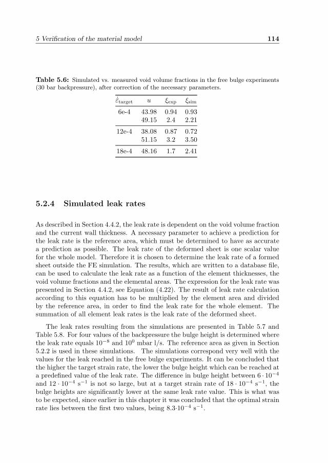
5 Verification of the material model 114
Table 5.6: Simulated vs. measured void volume fractions in the free bulge experiments(30 bar backpressure), after correction of the necessary parameters.
˙εtarget u ξexp ξsim
6e-4 43.98 0.94 0.9349.15 2.4 2.21
12e-4 38.08 0.87 0.7251.15 3.2 3.50
18e-4 48.16 1.7 2.41
5.2.4 Simulated leak rates
As described in Section 4.4.2, the leak rate is dependent on the void volume fractionand the current wall thickness. A necessary parameter to achieve a prediction forthe leak rate is the reference area, which must be determined to have as accuratea prediction as possible. The leak rate of the deformed sheet is one scalar valuefor the whole model. Therefore it is chosen to determine the leak rate of a formedsheet outside the FE simulation. The results, which are written to a database file,can be used to calculate the leak rate as a function of the element thicknesses, thevoid volume fractions and the elemental areas. The expression for the leak rate waspresented in Section 4.4.2, see Equation (4.22). The result of leak rate calculationaccording to this equation has to be multiplied by the element area and dividedby the reference area, in order to find the leak rate for the whole element. Thesummation of all element leak rates is the leak rate of the deformed sheet.
The leak rates resulting from the simulations are presented in Table 5.7 andTable 5.8. For four values of the backpressure the bulge height is determined wherethe leak rate equals 10−8 and 100 mbar l/s. The reference area as given in Section5.2.2 is used in these simulations. The simulations correspond very well with thevalues for the leak reached in the free bulge experiments. It can be concluded thatthe higher the target strain rate, the lower the bulge height which can be reached ata predefined value of the leak rate. The difference in bulge height between 6 · 10−4
and 12 · 10−4 s−1 is not so large, but at a target strain rate of 18 · 10−4 s−1, thebulge heights are significantly lower at the same leak rate value. This is what wasto be expected, since earlier in this chapter it was concluded that the optimal strainrate lies between the first two values, being 8.3·10−4 s−1.
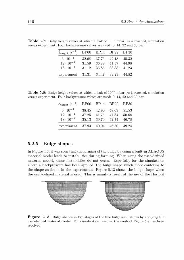
115 5.2 Free bulge simulations
Table 5.7: Bulge height values at which a leak of 10−8 mbar l/s is reached, simulationversus experiment. Four backpressure values are used: 0, 14, 22 and 30 bar
˙εtarget [s−1] BP00 BP14 BP22 BP30
6 · 10−4 32.68 37.76 42.18 45.3212 · 10−4 31.59 36.88 41.57 44.9818 · 10−4 31.12 35.86 38.88 41.23
experiment 31.31 34.47 39.23 44.82
Table 5.8: Bulge height values at which a leak of 10−1 mbar l/s is reached, simulationversus experiment. Four backpressure values are used: 0, 14, 22 and 30 bar
˙εtarget [s−1] BP00 BP14 BP22 BP30
6 · 10−4 38.45 42.90 48.09 51.5312 · 10−4 37.25 41.75 47.34 50.6818 · 10−4 35.13 39.79 42.74 46.78
experiment 37.93 40.04 46.50 49.24
5.2.5 Bulge shapes
In Figure 4.3, it was seen that the forming of the bulge by using a built-in ABAQUSmaterial model leads to instabilities during forming. When using the user-definedmaterial model, these instabilities do not occur. Especially for the simulationswhere a backpressure has been applied, the bulge shape much more conforms tothe shape as found in the experiments. Figure 5.13 shows the bulge shape whenthe user-defined material is used. This is mainly a result of the use of the Hosford
Figure 5.13: Bulge shapes in two stages of the free bulge simulations by applying theuser-defined material model. For visualization reasons, the mesh of Figure 5.8 has beenrevolved.
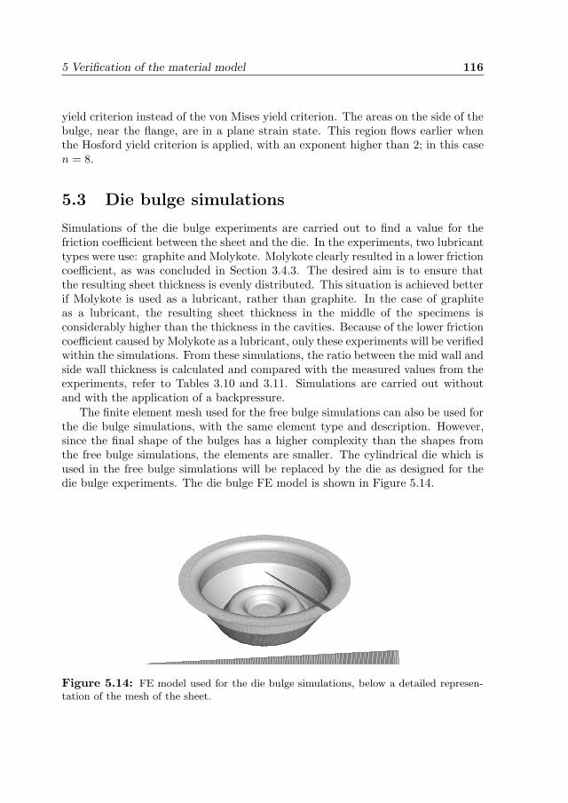
5 Verification of the material model 116
yield criterion instead of the von Mises yield criterion. The areas on the side of thebulge, near the flange, are in a plane strain state. This region flows earlier whenthe Hosford yield criterion is applied, with an exponent higher than 2; in this casen = 8.
5.3 Die bulge simulations
Simulations of the die bulge experiments are carried out to find a value for thefriction coefficient between the sheet and the die. In the experiments, two lubricanttypes were use: graphite and Molykote. Molykote clearly resulted in a lower frictioncoefficient, as was concluded in Section 3.4.3. The desired aim is to ensure thatthe resulting sheet thickness is evenly distributed. This situation is achieved betterif Molykote is used as a lubricant, rather than graphite. In the case of graphiteas a lubricant, the resulting sheet thickness in the middle of the specimens isconsiderably higher than the thickness in the cavities. Because of the lower frictioncoefficient caused by Molykote as a lubricant, only these experiments will be verifiedwithin the simulations. From these simulations, the ratio between the mid wall andside wall thickness is calculated and compared with the measured values from theexperiments, refer to Tables 3.10 and 3.11. Simulations are carried out withoutand with the application of a backpressure.
The finite element mesh used for the free bulge simulations can also be used forthe die bulge simulations, with the same element type and description. However,since the final shape of the bulges has a higher complexity than the shapes fromthe free bulge simulations, the elements are smaller. The cylindrical die which isused in the free bulge simulations will be replaced by the die as designed for thedie bulge experiments. The die bulge FE model is shown in Figure 5.14.
Figure 5.14: FE model used for the die bulge simulations, below a detailed represen-tation of the mesh of the sheet.
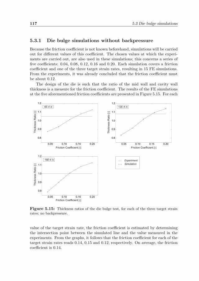
117 5.3 Die bulge simulations
5.3.1 Die bulge simulations without backpressure
Because the friction coefficient is not known beforehand, simulations will be carriedout for different values of this coefficient. The chosen values at which the experi-ments are carried out, are also used in these simulations; this concerns a series offive coefficients: 0.04, 0.08, 0.12, 0.16 and 0.20. Each simulation covers a frictioncoefficient and one of the three target strain rates, resulting in 15 FE simulations.From the experiments, it was already concluded that the friction coefficient mustbe about 0.12.
The design of the die is such that the ratio of the mid wall and cavity wallthickness is a measure for the friction coefficient. The results of the FE simulationsat the five aforementioned friction coefficients are presented in Figure 5.15. For each
0.05 0.10 0.15 0.20
0.8
0.9
1.0
1.1
1.2
0.05 0.10 0.15 0.20
0.8
0.9
1.0
1.1
1.2
0.05 0.10 0.15 0.20
0.8
0.9
1.0
1.1
1.2
Friction Coefficient [-] Friction Coefficient [-]
Friction Coefficient [-]
Th
ickn
ess R
atio
[-]
Th
ickn
ess R
atio
[-]
Th
ickn
ess R
atio
[-]
18E-4 /s
12E-4 /s6E-4 /s
ExperimentSimulation
Figure 5.15: Thickness ratios of the die bulge test, for each of the three target strainrates; no backpressure.
value of the target strain rate, the friction coefficient is estimated by determiningthe intersection point between the simulated line and the value measured in theexperiments. From the graphs, it follows that the friction coefficient for each of thetarget strain rates reads 0.14, 0.15 and 0.12, respectively. On average, the frictioncoefficient is 0.14.
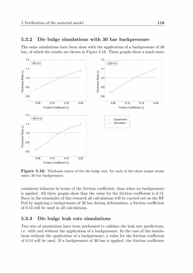
5 Verification of the material model 118
5.3.2 Die bulge simulations with 30 bar backpressure
The same simulations have been done with the application of a backpressure of 30bar, of which the results are shown in Figure 5.16. These graphs show a much more
0.05 0.10 0.15 0.20
0.8
0.9
1.0
1.1
1.2
0.05 0.10 0.15 0.20
0.8
0.9
1.0
1.1
1.2
0.05 0.10 0.15 0.20
0.8
0.9
1.0
1.1
1.2
18E-4 /s
12E-4 /s6E-4 /s
ExperimentSimulation
Friction Coefficient [-]
Th
ickn
ess R
atio
[-]
Friction Coefficient [-]
Th
ickn
ess R
atio
[-]
Friction Coefficient [-]
Th
ickn
ess R
atio
[-]
Figure 5.16: Thickness ratios of the die bulge test, for each of the three target strainrates; 30 bar backpressure.
consistent behavior in terms of the friction coefficient, than when no backpressureis applied. All three graphs show that the value for the friction coefficient is 0.13.Since in the remainder of this research all calculations will be carried out on the RFFoil by applying a backpressure of 30 bar during deformation, a friction coefficientof 0.13 will be used in all calculations.
5.3.3 Die bulge leak rate simulations
Two sets of simulations have been performed to validate the leak rate predictions,i.e. with and without the application of a backpressure. In the case of the simula-tions without the application of a backpressure, a value for the friction coefficientof 0.14 will be used. If a backpressure of 30 bar is applied, the friction coefficient
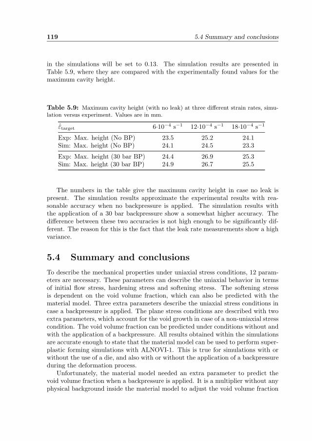
119 5.4 Summary and conclusions
in the simulations will be set to 0.13. The simulation results are presented inTable 5.9, where they are compared with the experimentally found values for themaximum cavity height.
Table 5.9: Maximum cavity height (with no leak) at three different strain rates, simu-lation versus experiment. Values are in mm.
˙εtarget 6·10−4 s−1 12·10−4 s−1 18·10−4 s−1
Exp: Max. height (No BP) 23.5 25.2 24.1Sim: Max. height (No BP) 24.1 24.5 23.3
Exp: Max. height (30 bar BP) 24.4 26.9 25.3Sim: Max. height (30 bar BP) 24.9 26.7 25.5
The numbers in the table give the maximum cavity height in case no leak ispresent. The simulation results approximate the experimental results with rea-sonable accuracy when no backpressure is applied. The simulation results withthe application of a 30 bar backpressure show a somewhat higher accuracy. Thedifference between these two accuracies is not high enough to be significantly dif-ferent. The reason for this is the fact that the leak rate measurements show a highvariance.
5.4 Summary and conclusions
To describe the mechanical properties under uniaxial stress conditions, 12 param-eters are necessary. These parameters can describe the uniaxial behavior in termsof initial flow stress, hardening stress and softening stress. The softening stressis dependent on the void volume fraction, which can also be predicted with thematerial model. Three extra parameters describe the uniaxial stress conditions incase a backpressure is applied. The plane stress conditions are described with twoextra parameters, which account for the void growth in case of a non-uniaxial stresscondition. The void volume fraction can be predicted under conditions without andwith the application of a backpressure. All results obtained within the simulationsare accurate enough to state that the material model can be used to perform super-plastic forming simulations with ALNOVI-1. This is true for simulations with orwithout the use of a die, and also with or without the application of a backpressureduring the deformation process.
Unfortunately, the material model needed an extra parameter to predict thevoid volume fraction when a backpressure is applied. It is a multiplier without anyphysical background inside the material model to adjust the void volume fraction
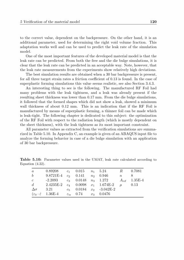
5 Verification of the material model 120
to the correct value, dependent on the backpressure. On the other hand, it is anadditional parameter, used for determining the right void volume fraction. Thisadaptation works well and can be used to predict the leak rate of the simulationmodel.
One of the most important features of the developed material model is that theleak rate can be predicted. From both the free and the die bulge simulations, it isclear that the leak rate can be predicted in an acceptable way. Note, however, thatthe leak rate measurements from the experiments show relatively high deviations.
The best simulation results are obtained when a 30 bar backpressure is present,for all three target strain rates a friction coefficient of 0.13 is found. In the case ofsuperplastic forming simulations this value seems realistic, see also Section 3.4.3.
An interesting thing to see is the following. The manufactured RF Foil hadmany problems with the leak tightness, and a leak was already present if theresulting sheet thickness was lower than 0.17 mm. From the die bulge simulations,it followed that the formed shapes which did not show a leak, showed a minimumwall thickness of about 0.12 mm. This is an indication that if the RF Foil ismanufactured by means of superplastic forming, a thinner foil can be made whichis leak-tight. The following chapter is dedicated to this subject: the optimizationof the RF Foil with respect to the radiation length (which is mostly dependent onthe sheet thickness), with the leak tightness as its most important constraint.
All parameter values as extracted from the verification simulations are summa-rized in Table 5.10. In Appendix C, an example is given of an ABAQUS input file toanalyze the forming behavior in case of a die bulge simulation with an applicationof 30 bar backpressure.
Table 5.10: Parameter values used in the UMAT, leak rate calculated according toEquation (4.22).
a 0.89208 c1 0.015 n1 5.24 R 0.7081b 9.8721E-4 c2 0.141 n2 0.946 n 8c -2.2093 c3 0.0148 n3 1.272 Aref 1.35E-4d 2.4235E-2 c4 0.0098 x1 1.674E-2 μ 0.13Δσ 3.21 c5 0.0184 x2 -3.042E-2(ε0 · ε 1.36E-4 εtr 0.74 x3 0.0476
6. Optimization of the RF Foil
In Chapter 1, the properties of the current RF Foil, to be used in the LHCb VeLodetector, are discussed. The current design is the product of a trial-and-errorprocedure, which resulted in an RF Foil that met the requirements. However, thisis believed not to be an optimal design. If the percentual radiation length of theRF Foil could be made smaller, then the measurement error of the detectors placedin the RF Box (to recall: The RF Foil is the top sheet of the RF Box) would besmaller. This reduction in radiation length, which means in general a reduction inthe resulting sheet thickness, is restricted to a set of requirements, also mentionedin Chapter 1.
In the optimization problem of the RF Foil, the percentual radiation length ischosen as the objective function. In simple terms, this is the probability that aparticle trajectory is measured incorrectly. This objective function must be mini-mized by finding optimal settings of the design variables while satisfying a set ofconstraints. Section 6.1 gives a general overview and some solution algorithms usedin optimization theory.
A program developed at the Twente University by M. Bonte, called OptForm,uses an optimization methodology that will be used in the RF Foil optimizationprocedure. One of the mathematical techniques that is used in the optimizationalgorithm is the Response Surface Methodology (RSM) [11, 58]. A description ofthe optimization strategy will be presented in Section 6.2.
In order to calculate the percentual radiation length (the objective function), aprocedure has been programmed which is based on the finite element model of thedeformed sheet. This radiation length is a direct result of the averaged traversedpath of a particle through the sheet, emerging from a fixed point. The calculationprocedure of the radiation length is described in Section 6.3.
The value of the objective function is determined by the settings of the designvariables. In order to have a limited number of design variables, the design ofthe current RF Foil has to be parameterized. The settings of the design variablesof this parameterized model determine the value of the objective function. Thisobjective function value must be determined by means of an FE calculation. Theparameterization of the RF Foil is covered in Section 6.4.
The ranges of the design variables are bounded, for instance, due to the fact
121
6 Optimization of the RF Foil 122
that the RF Box must contain a well-defined set of silicon detectors. Impossible orlimited combinations of design variable settings result in a set of explicit constraints.More complex defined constraints, such as the leak rate or the mechanical stiffness,are called implicit constraints. The value of these constraints must be determinedby means of FE analyses. The constraints on the RF Foil are described in Section6.5.
All FE simulations to be carried out on the RF Foil to determine the value of theresponses are computationally expensive if the whole RF Foil (or a quarter becauseof double symmetry) has to be analyzed for each design. Therefore, a simplifiedmodel is used which represents the whole RF Foil. Analyzing this simplified modelwill save a considerable amount of simulation time. The results of the simulationson this simplified model will be translated to corresponding results for the wholeRF Foil. The translation procedure is discussed together with the discussion of thedesign variables and the constraints in Section 6.4 and 6.5.
The objective function, design variables and constraints are used as an inputfor OptForm. This program is used to help in developing an optimized RF Foil.This is the subject of Section 6.6.
6.1 Optimization theory: a brief description
This section presents a short introduction to optimization theory, in so far applica-ble to the optimization problem concerning the RF Foil. This means that a singleobjective function is sufficient to deal with. The value of this function is determinedby the value of the design variables, subject to implicit or explicit constraints.
6.1.1 Description of the optimization problem
Figure 6.1 shows an example of an optimization problem in a graph, where twodesign variables x1 and x2 determine the value of the objective function f . In thearea which is bounded by the five constraints g1 to g5, the minimum value of theobjective function is found to be equal to fopt. This is the case if the two designvariables are equal to x∗
1 and x∗2.
The procedure to find the optimal values for the design variables must in manycases be determined numerically. An optimization algorithm has to determine inan iterative way where the optimum is situated. Figure 6.2 depicts the generaloptimization procedure to reach a satisfactory minimum value of the objectivefunction. Starting from an initial design, an optimization algorithm should improvethe design until a minimum value for the objective function is found. In that case,the resulting design can be considered optimal.
Three questions can be asked:
• how do you choose an initial design? If the design is a technological innova-tion, a solution for this question is hard to find, since there is no experience
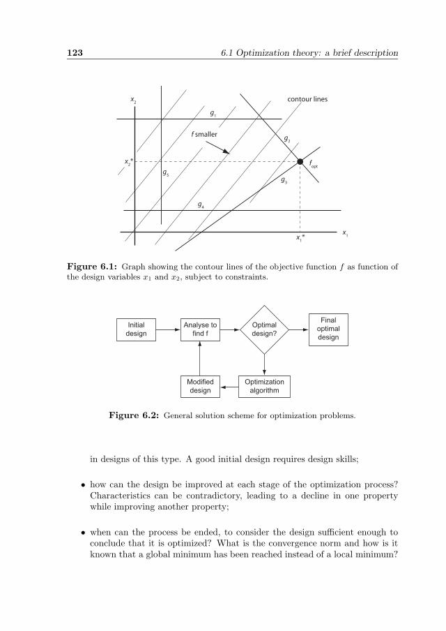
123 6.1 Optimization theory: a brief description
x1
x2
g1
g2
g3
g4
g5
f smaller
contour lines
fopt
x1*
x2*
Figure 6.1: Graph showing the contour lines of the objective function f as function ofthe design variables x1 and x2, subject to constraints.
Initial
design
Analyse to
find f
Final
optimal
design
Optimization
algorithm
Modified
design
Optimal
design?
Figure 6.2: General solution scheme for optimization problems.
in designs of this type. A good initial design requires design skills;
• how can the design be improved at each stage of the optimization process?Characteristics can be contradictory, leading to a decline in one propertywhile improving another property;
• when can the process be ended, to consider the design sufficient enough toconclude that it is optimized? What is the convergence norm and how is itknown that a global minimum has been reached instead of a local minimum?
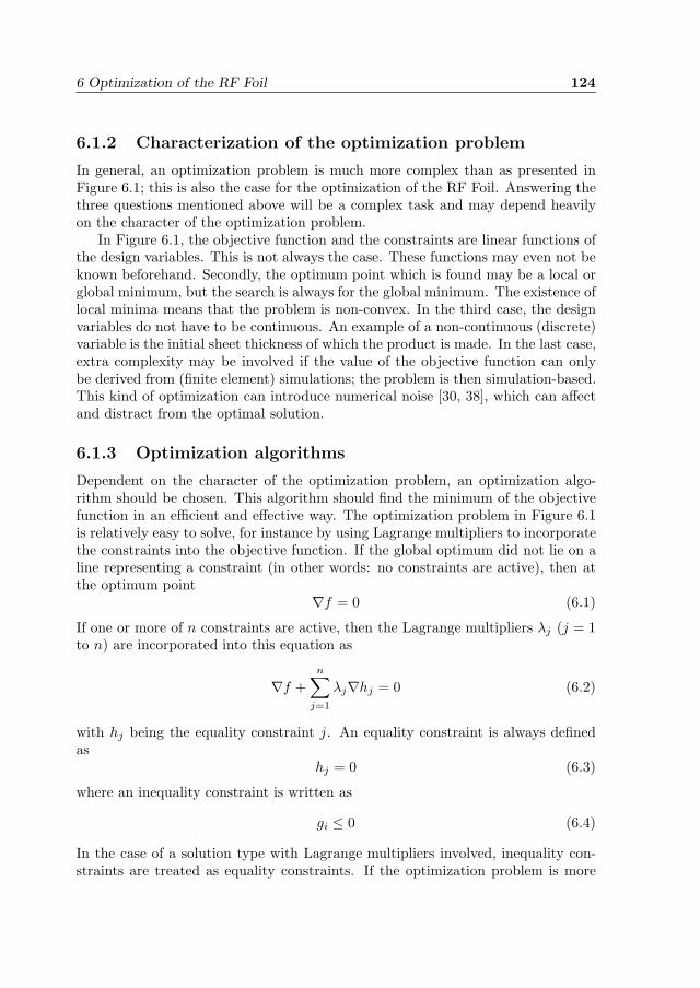
6 Optimization of the RF Foil 124
6.1.2 Characterization of the optimization problem
In general, an optimization problem is much more complex than as presented inFigure 6.1; this is also the case for the optimization of the RF Foil. Answering thethree questions mentioned above will be a complex task and may depend heavilyon the character of the optimization problem.
In Figure 6.1, the objective function and the constraints are linear functions ofthe design variables. This is not always the case. These functions may even not beknown beforehand. Secondly, the optimum point which is found may be a local orglobal minimum, but the search is always for the global minimum. The existence oflocal minima means that the problem is non-convex. In the third case, the designvariables do not have to be continuous. An example of a non-continuous (discrete)variable is the initial sheet thickness of which the product is made. In the last case,extra complexity may be involved if the value of the objective function can onlybe derived from (finite element) simulations; the problem is then simulation-based.This kind of optimization can introduce numerical noise [30, 38], which can affectand distract from the optimal solution.
6.1.3 Optimization algorithms
Dependent on the character of the optimization problem, an optimization algo-rithm should be chosen. This algorithm should find the minimum of the objectivefunction in an efficient and effective way. The optimization problem in Figure 6.1is relatively easy to solve, for instance by using Lagrange multipliers to incorporatethe constraints into the objective function. If the global optimum did not lie on aline representing a constraint (in other words: no constraints are active), then atthe optimum point
∇f = 0 (6.1)
If one or more of n constraints are active, then the Lagrange multipliers λj (j = 1to n) are incorporated into this equation as
∇f +n∑
j=1
λj∇hj = 0 (6.2)
with hj being the equality constraint j. An equality constraint is always definedas
hj = 0 (6.3)
where an inequality constraint is written as
gi ≤ 0 (6.4)
In the case of a solution type with Lagrange multipliers involved, inequality con-straints are treated as equality constraints. If the optimization problem is more
125 6.1 Optimization theory: a brief description
complex, several other algorithms are available to solve this problem. A few arementioned in [1, 77], and briefly described below.
Method of Conjugate Directions This method is based on the method ofSteepest Descent, where in a point defined by a set of design variables not onlythe objective function is determined, but also the derivative of this function withrespect to the design variables. The method of Steepest Descent gives a searchdirection for the improved design. This method does not converge very fast, theMethod of Conjugate Directions results in faster convergence. Here, not only thefirst derivatives are used, but also the second derivatives (Hessian). This givesbetter information about the search direction for the improved design.
This method works very well if the objective function is quadratically dependenton the design variables, but this method can quickly lose its accuracy if higher orderdependencies are present. This method is a line search method, where the searchdirection is determined first, after which the search distance is determined.
Trust Region methods Around a point representing a design, a quadraticmodel is built of the objective function. This quadratic model is believed to beaccurate enough within a region, called the Trust Region. Within this region, thequadratic model is minimized. At this new minimized point (i.e. the new design),the objective function value is evaluated and compared with the value accordingto the quadratic model. The deviation between these two numbers determines theaccuracy of the quadratic model and the Trust Region size in the next iteration.
In the Trust Region method, the search distance is determined first, after whichthe search direction is calculated. So, this is contrary to the line search method.The main drawback of the Trust Region Method is if the quadratic model is notadequate enough, many iterations may be necessary to obtain considerably smallersubspaces.
Genetic algorithms Genetic algorithms are based on the principle of survivalof the fittest. It is an evolutionary algorithm where there is not one initial design,but a population of initial designs. All the members of this population have theirown value for the objective function. The members of this population are calledthe first generation. In the second generation, also a set of designs, for each of thenew designs (’children’) two parents are chosen. The smaller the objective functionof a member of the first generation, the higher the chance that it will become aparent for the second generation.
This method is inspired by the evolution theory, and can be extended withcharacteristics from this theory, as mutations and cross-overs. Each next generationwill generally consist of fitter members than the previous generation. The maindrawback of this method is that many objective function evaluations are necessaryin each generation to derive the members of the next generation.
6 Optimization of the RF Foil 126
Metamodeling techniques These statistical optimization methods can be usedfor very complex optimization problems. They are sequential in nature, that meansthat a fixed sequence of steps has to be taken to improve the design in order to findthe optimal design with the lowest value of the objective function. The first step isa screening step to explore the bounds of the design space. This step is also used todetermine which design variables have the highest impact on the objective functionvalue. In the second step, a so-called Design Of Experiments (DOE) is established,consisting of a set of well-defined designs within the design space. After evaluatingthe objective function values of these designs, a series of expressions can be fittedthrough these points (designs). Statistical tools are used to test the validity ofthe expressions. The minimum in the expression with the highest quality of fitis searched for (or more minima if there are local minima), and a new DOE maybe established in a smaller region. One of the mathematical tools to describe ametamodel is the Response Surface Methodology (RSM).
This method requires a considerable amount of objective function evaluations,so it is of crucial importance that an effective DOE is made. The nature of RSM isthat this amount of evaluations can give much information on the way the objectivebehaves under a variation in the design variables. A major disadvantage arises ifthe equations to fit the data are far from reality.
The main reasons to choose this method in this project are
• a metamodeling techniques is a relatively effective method to distinguishbetween local and global minima;
• metamodeling techniques are effective methods for complex optimizationproblems where the value of the objective function is not an analytical func-tion, or if this function is not known;
• with the application of e.g. genetic algorithms, the aspect ’luck’ plays a role.This is far less likely if a mathematical tool such as RSM is used.
The next section describes more elaborately the theory of RSM.
6.2 Optimization strategy
Each set of design variables results in one value for the objective function, inResponse Surface Methodology (RSM) [11, 58] also called response. The RSMcreates a number of designs for which the response is evaluated. The whole set ofresponses can be graphically depicted, for instance if only two design variables areinfluencing the response. Fig 6.3 shows an example of the response y as functionof two variables x1 and x2. A predetermined space defined by upper and lowerlimits on x1 and x2 is explored in a series of points. A surface function will then befitted through the obtained response values (objective function and constraints),
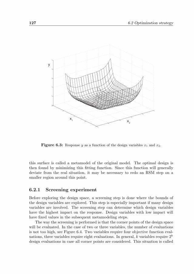
127 6.2 Optimization strategy
x2
x1
y
Figure 6.3: Response y as a function of the design variables x1 and x2.
this surface is called a metamodel of the original model. The optimal design isthen found by minimizing this fitting function. Since this function will generallydeviate from the real situation, it may be necessary to redo an RSM step on asmaller region around this point.
6.2.1 Screening experiment
Before exploring the design space, a screening step is done where the bounds ofthe design variables are explored. This step is especially important if many designvariables are involved. The screening step can determine which design variableshave the highest impact on the response. Design variables with low impact willhave fixed values in the subsequent metamodeling steps.
The way the screening is performed is that the corner points of the design spacewill be evaluated. In the case of two or three variables, the number of evaluationsis not too high, see Figure 6.4. Two variables require four objective function eval-uations, three variables require eight evaluations. In general, k variables require 2k
design evaluations in case all corner points are considered. This situation is called
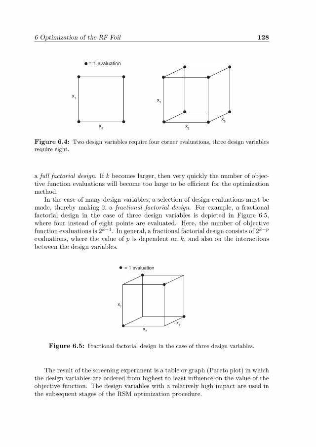
6 Optimization of the RF Foil 128
x1
x2
x1
x2
x3
= 1 evaluation
Figure 6.4: Two design variables require four corner evaluations, three design variablesrequire eight.
a full factorial design. If k becomes larger, then very quickly the number of objec-tive function evaluations will become too large to be efficient for the optimizationmethod.
In the case of many design variables, a selection of design evaluations must bemade, thereby making it a fractional factorial design. For example, a fractionalfactorial design in the case of three design variables is depicted in Figure 6.5,where four instead of eight points are evaluated. Here, the number of objectivefunction evaluations is 2k−1. In general, a fractional factorial design consists of 2k−p
evaluations, where the value of p is dependent on k, and also on the interactionsbetween the design variables.
x1
x2
x3
= 1 evaluation
Figure 6.5: Fractional factorial design in the case of three design variables.
The result of the screening experiment is a table or graph (Pareto plot) in whichthe design variables are ordered from highest to least influence on the value of theobjective function. The design variables with a relatively high impact are used inthe subsequent stages of the RSM optimization procedure.
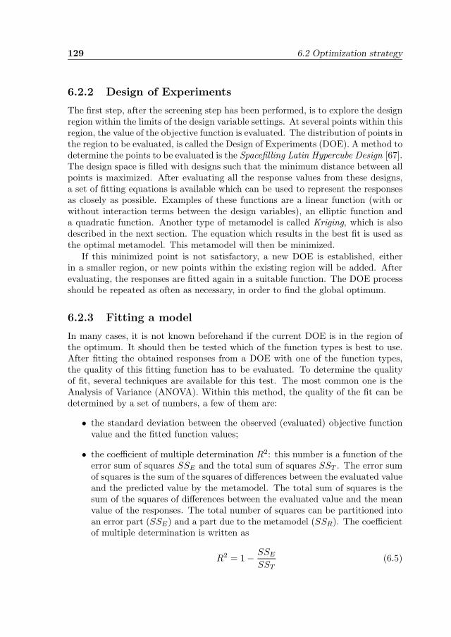
129 6.2 Optimization strategy
6.2.2 Design of Experiments
The first step, after the screening step has been performed, is to explore the designregion within the limits of the design variable settings. At several points within thisregion, the value of the objective function is evaluated. The distribution of points inthe region to be evaluated, is called the Design of Experiments (DOE). A method todetermine the points to be evaluated is the Spacefilling Latin Hypercube Design [67].The design space is filled with designs such that the minimum distance between allpoints is maximized. After evaluating all the response values from these designs,a set of fitting equations is available which can be used to represent the responsesas closely as possible. Examples of these functions are a linear function (with orwithout interaction terms between the design variables), an elliptic function anda quadratic function. Another type of metamodel is called Kriging, which is alsodescribed in the next section. The equation which results in the best fit is used asthe optimal metamodel. This metamodel will then be minimized.
If this minimized point is not satisfactory, a new DOE is established, eitherin a smaller region, or new points within the existing region will be added. Afterevaluating, the responses are fitted again in a suitable function. The DOE processshould be repeated as often as necessary, in order to find the global optimum.
6.2.3 Fitting a model
In many cases, it is not known beforehand if the current DOE is in the region ofthe optimum. It should then be tested which of the function types is best to use.After fitting the obtained responses from a DOE with one of the function types,the quality of this fitting function has to be evaluated. To determine the qualityof fit, several techniques are available for this test. The most common one is theAnalysis of Variance (ANOVA). Within this method, the quality of the fit can bedetermined by a set of numbers, a few of them are:
• the standard deviation between the observed (evaluated) objective functionvalue and the fitted function values;
• the coefficient of multiple determination R2: this number is a function of theerror sum of squares SSE and the total sum of squares SST . The error sumof squares is the sum of the squares of differences between the evaluated valueand the predicted value by the metamodel. The total sum of squares is thesum of the squares of differences between the evaluated value and the meanvalue of the responses. The total number of squares can be partitioned intoan error part (SSE) and a part due to the metamodel (SSR). The coefficientof multiple determination is written as
R2 = 1 − SSE
SST(6.5)
6 Optimization of the RF Foil 130
The closer this value to 1, the better the fit;
• because the coefficient of multiple determination increases when more termsin the metamodel are added, this value is not always a good measure. There-fore an adjusted value is defined, which does not necessarily increase if thenumber of terms is increased, this is called R2
adj. It is even possible that thisvalue decreases if unnecessary terms are added. This value is defined by
R2adj = 1 − n − 1
n − p(1 − R2) (6.6)
where n is the total number of observations and p is the number of modelparameters (degrees of freedom) for the function type to be used. The de-nominator in Equation (6.6) decreases with the number of model parameters,the term (1 − R2) increases with the number of model parameters;
• the RMSE (Root Mean Square Error) value: this is a value which is depen-dent on SSE and is defined as
RMSE =
√SSE
n − k − 1(6.7)
where k is the number of regression variables. The RMSE should be as lowas possible, indicating that the squared sum of errors is low, combined witha low number of regression parameters.
Kriging A function fit like a linear or a quadratic equation always shows an error,not only in the unknown points, but also in the known points where the objectivefunction values have been evaluated. Kriging interpolation is a technique wherethe fitted function goes through the known points, so the error in these points iszero. At unknown values in between the known values for the objective function,the value f∗ is estimated as a function of (all n) known values as
f∗ =n∑
i=1
λifi (6.8)
where λi is a weight factor for the known value fi, the sum of all these weight factorsis equal to 1. In theory, all n function values are taken into account but this cantake too much effort if n is large. Therefore, a limited number of values of pointsin the vicinity of the point in consideration is taken into account. Figure 6.6 showsthe difference between an RSM (in this case quadratic) and a Kriging interpolationfunction. Also, a gray colored confidence interval is shown for the Kriging procedurefor the intermediate points. This can give insight in the phenomenon whether alocal or the global minimum is situated between two known points. In the case of
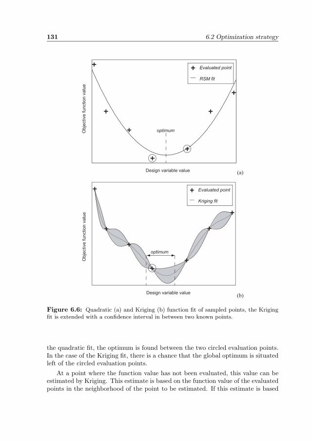
131 6.2 Optimization strategy
Design variable value
Ob
jective
fu
nctio
n v
alu
e
Design variable value
Ob
jective
fu
nctio
n v
alu
e
Evaluated point
RSM fit
Evaluated point
Kriging fit
(a)
(b)
optimum
optimum
Figure 6.6: Quadratic (a) and Kriging (b) function fit of sampled points, the Krigingfit is extended with a confidence interval in between two known points.
the quadratic fit, the optimum is found between the two circled evaluation points.In the case of the Kriging fit, there is a chance that the global optimum is situatedleft of the circled evaluation points.
At a point where the function value has not been evaluated, this value can beestimated by Kriging. This estimate is based on the function value of the evaluatedpoints in the neighborhood of the point to be estimated. If this estimate is based
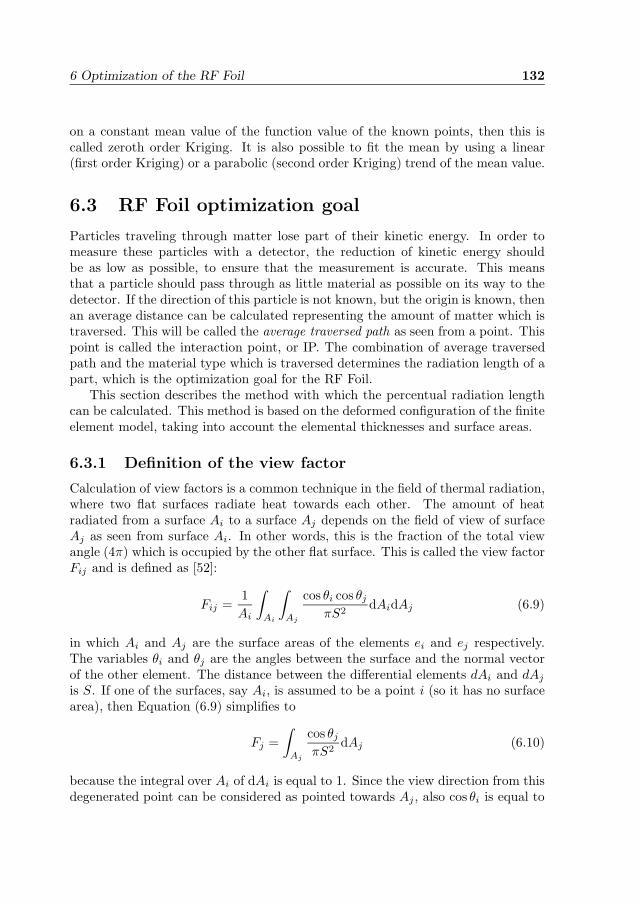
6 Optimization of the RF Foil 132
on a constant mean value of the function value of the known points, then this iscalled zeroth order Kriging. It is also possible to fit the mean by using a linear(first order Kriging) or a parabolic (second order Kriging) trend of the mean value.
6.3 RF Foil optimization goal
Particles traveling through matter lose part of their kinetic energy. In order tomeasure these particles with a detector, the reduction of kinetic energy shouldbe as low as possible, to ensure that the measurement is accurate. This meansthat a particle should pass through as little material as possible on its way to thedetector. If the direction of this particle is not known, but the origin is known, thenan average distance can be calculated representing the amount of matter which istraversed. This will be called the average traversed path as seen from a point. Thispoint is called the interaction point, or IP. The combination of average traversedpath and the material type which is traversed determines the radiation length of apart, which is the optimization goal for the RF Foil.
This section describes the method with which the percentual radiation lengthcan be calculated. This method is based on the deformed configuration of the finiteelement model, taking into account the elemental thicknesses and surface areas.
6.3.1 Definition of the view factor
Calculation of view factors is a common technique in the field of thermal radiation,where two flat surfaces radiate heat towards each other. The amount of heatradiated from a surface Ai to a surface Aj depends on the field of view of surfaceAj as seen from surface Ai. In other words, this is the fraction of the total viewangle (4π) which is occupied by the other flat surface. This is called the view factorFij and is defined as [52]:
Fij =1Ai
∫Ai
∫Aj
cos θi cos θj
πS2dAidAj (6.9)
in which Ai and Aj are the surface areas of the elements ei and ej respectively.The variables θi and θj are the angles between the surface and the normal vectorof the other element. The distance between the differential elements dAi and dAj
is S. If one of the surfaces, say Ai, is assumed to be a point i (so it has no surfacearea), then Equation (6.9) simplifies to
Fj =∫
Aj
cos θj
πS2dAj (6.10)
because the integral over Ai of dAi is equal to 1. Since the view direction from thisdegenerated point can be considered as pointed towards Aj , also cos θi is equal to

133 6.3 RF Foil optimization goal
1. If Aj is a small enough surface with respect to the distance S to this point i,for instance if this surface is a finite element far enough from i, then the integralover Aj of dAj is equal to its surface area Aj , so:
Fj =Aj cos θj
πS2(6.11)
The distance S should represent the average distance from point i to the surfaceAj . Taking the midpoint of Aj can give inaccurate results, this can be seen if thenormal of the element is pointed towards i. The midpoint is the closest point, thisgives a systematic error in the distance calculation. A better method is to calculatean average distance based on the midpoint and the four corner points (in the caseof quadrilateral elements) as
S =
∑4j=1(d
ej + 4de
m)8
(6.12)
where dej is the distance from point i to the corner point j of element e and de
m isthe distance from point i to the midpoint of element e.
6.3.2 Calculation of the averaged traversed path
The average traversed path t is dependent on the view factor and on the thicknessof the traversed element. Figure 6.7 shows a particle emerging from the interactionpoint IP, crossing element e. The picture shows a 2-dimensional situation. Thetraversed path through the element is tθ. This path length is dependent on theorientation φ of the element with respect to IP and the angle θe. If the traversed
IP
particle track
φ
α θe
t
tθ
Figure 6.7: Particle crossing element e, the traversed path is tθ.
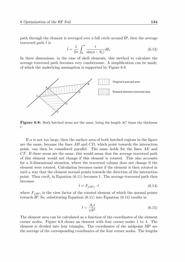
6 Optimization of the RF Foil 134
path through the element is averaged over a full circle around IP, then the averagetraversed path t is
t =12π
∫ α
0
t
sin(φ − θe)dθe (6.13)
In three dimensions, in the case of shell elements, this method to calculate theaverage traversed path becomes very cumbersome. A simplification can be made,of which the underlying assumption is supported by Figure 6.8.
Original traversed area
Rotated element traversed area
A
F
E
D
B
C
Figure 6.8: Both hatched areas are the same, being the length AC times the thicknesst.
If α is not too large, then the surface area of both hatched regions in the figureare the same, because the lines AB and CD, which point towards the interactionpoint, can then be considered parallel. The same holds for the lines AE andCF . If these areas are the same, this would mean that the average traversed pathof this element would not change if this element is rotated. This also accountsfor a 3-dimensional situation, where the traversed volume does not change if theelement were rotated. Calculation becomes easier if the element is then rotated insuch a way that the element normal points towards the direction of the interactionpoint. Then cos θj in Equation (6.11) becomes 1. The average traversed path thenbecomes
t = Fj(IP) · t (6.14)
where Fj(IP) is the view factor of the rotated element of which the normal pointstowards IP. So, substituting Equation (6.11) into Equation (6.14) results in
t =Ajt
πS2(6.15)
The element area can be calculated as a function of the coordinates of the elementcorner nodes. Figure 6.9 shows an element with four corner nodes 1 to 4. Theelement is divided into four triangles. The coordinates of the midpoint MP arethe average of the corresponding coordinates of the four corner nodes. The lengths
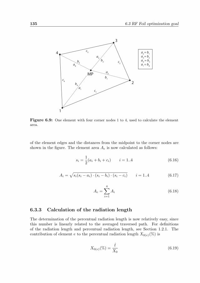
135 6.3 RF Foil optimization goal
1
2
3
4
MP
a1
b1
c1
a2
b2 c
2
a3
b3
c3
a4
b4
c4
a2 = b
1
a3 = b
2
a4 = b
3
a1 = b
4
Figure 6.9: One element with four corner nodes 1 to 4, used to calculate the elementarea.
of the element edges and the distances from the midpoint to the corner nodes areshown in the figure. The element area Ae is now calculated as follows:
si =12(ai + bi + ci) i = 1..4 (6.16)
Ai =√
si(si − ai) · (si − bi) · (si − ci) i = 1..4 (6.17)
Ae =4∑
i=1
Ai (6.18)
6.3.3 Calculation of the radiation length
The determination of the percentual radiation length is now relatively easy, sincethis number is linearly related to the averaged traversed path. For definitionsof the radiation length and percentual radiation length, see Section 1.2.1. Thecontribution of element e to the percentual radiation length X0(e)(%) is
X0(e)(%) =t
X0(6.19)
6 Optimization of the RF Foil 136
where X0 is the material radiation length, which is 89 mm for aluminum. Theoverall percentual radiation length of the deformed structure is
X0(%) =#elements∑
e=1
X0(e)(%) (6.20)
The value of X0(%) is the number which has to be minimized. In other words: theobjective function is Fobj = X0(%).
6.4 RF Foil design variables
Since the design of the RF Box has been merely a process of trial and error, thedimensioning of this box is not suitable for parameterization. There are too manygeometric entities to make the RF Box an efficient design to be used in an op-timization procedure. This section describes a way to parameterize the RF Box,in particular the RF Foil, to reduce the number of design variables. In Chapter1, it was explained that the RF Foil is the top sheet of the RF Box. The maincharacteristics of the RF Box must be maintained, in order to fulfill its main func-tions (containing the detectors, minimizing wake field suppression). In this section,the parameterization is described step by step, thereby producing a list of designvariables to be used in the optimization procedure.
6.4.1 Dimensioning of the RF Foil
The box, especially the RF Foil, should consist of a set of parameters which mainlycharacterize the geometry. The dimensioning of the box must be such that it cancontain the silicon detectors. Two rows of these detectors, each in its own RF Box,should overlap when two boxes are situated correctly with respect to each other.An assembly of two of these boxes should leave a free channel for the acceleratorbeam to pass through.
Figure 6.10 shows how the geometry can be parameterized, a quarter of thesimplified foil has been displayed, due to double symmetry of the foil. Also, forsimulation efficiency reasons, not the whole length of the foil is modeled, but onlya model which is comparable to the one which was shown in Figure 1.5. Twodimensions in the figure are not a variable. One fixed dimension is the pitchfrom detector to detector, which is 30 mm. The other fixed dimension is due tothe silicon detector dimensions. The dimensions as shown in the figure have thefollowing functions and limits:
• The dimension H1 is the corrugation height. The minimum height is deter-mined by the positioning of the silicon sensors. This height is the same asin the current design of the RF Foil, i.e. 10 mm. The maximum corrugation
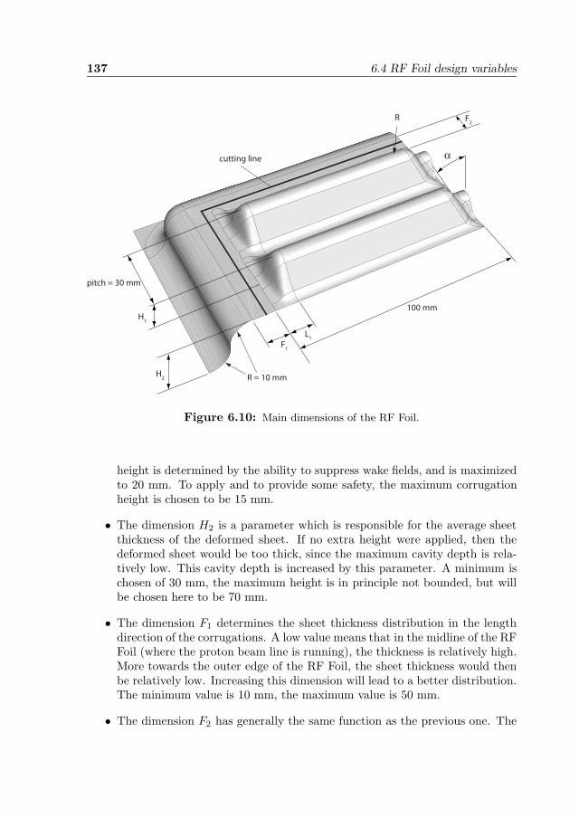
137 6.4 RF Foil design variables
pitch = 30 mm
H1
H2
R
F1
L1
α
F2
100 mm
cutting line
R = 10 mm
Figure 6.10: Main dimensions of the RF Foil.
height is determined by the ability to suppress wake fields, and is maximizedto 20 mm. To apply and to provide some safety, the maximum corrugationheight is chosen to be 15 mm.
• The dimension H2 is a parameter which is responsible for the average sheetthickness of the deformed sheet. If no extra height were applied, then thedeformed sheet would be too thick, since the maximum cavity depth is rela-tively low. This cavity depth is increased by this parameter. A minimum ischosen of 30 mm, the maximum height is in principle not bounded, but willbe chosen here to be 70 mm.
• The dimension F1 determines the sheet thickness distribution in the lengthdirection of the corrugations. A low value means that in the midline of the RFFoil (where the proton beam line is running), the thickness is relatively high.More towards the outer edge of the RF Foil, the sheet thickness would thenbe relatively low. Increasing this dimension will lead to a better distribution.The minimum value is 10 mm, the maximum value is 50 mm.
• The dimension F2 has generally the same function as the previous one. The
6 Optimization of the RF Foil 138
difference is that this dimension mainly takes care of the thickness distribu-tion between the separate corrugations. Especially the thickness in the firstcorrugation is determined by this dimension. Just as with F1, the range ofthis dimension is 10 to 50 mm.
• The dimension α has a more local function. It is the draft angle at the endcapside at the position of the beam line. This dimension has an influence on thelocal thickness in the top end of the corrugations. The minimum angle is 10o,the maximum value is 30o. Making this angle larger will result in missing toomuch detection space.
• The dimension L1 has the same function as α, but then on the other endcapside of the corrugations. This dimension ranges from 10 to 15 mm, keepingin mind the geometry of the detecting silicon sensors.
• The dimension R is the radius of the long side of the corrugations. Since thepitch between the corrugations is fixed at 30 mm, this dimension is not onlya fillet radius, but it also has an effect on the draft angle on the side walls ofthe corrugations. The radius R ranges between 4 and 6 mm.
The model shown in Figure 6.10 has to be cut along the bold lines to result in thepart that will contribute to the RF Foil. So, the dimensions H2, F1 and F2 areonly used to obtain a well-defined thickness distribution within the area boundedby these bold lines. The dimensions of the trimmed area are 105 x 65 mm.
6.4.2 Radiation length of the simplified model
The model shown in Figure 6.10 shows a simplified version of the full RF Foil. Allcalculations concerning the optimization of the RF Foil will be carried out withthis simplified model. The results in terms of the radiation length of the simplifiedmodel should be translated into a radiation length of the full RF Foil. This isdone by determining a multiplication factor. The radiation length of the RF Foilis then calculated by multiplying the radiation length of the simplified model bythis factor.
The radiation length of the simplified model is only determined for the partthat falls within the area that contributes to the RF Foil (105 x 65 mm). The fullRF Foil has 23 instead of four corrugations, so the total surface area is (23/4) timeslarger than the surface area of the simplified model. This does not mean that theradiation length is (23/4) times larger for the full RF Foil, since a large part of thisfoil is situated relatively far away from the interaction point. This means that forequal surface areas, the view factor at these higher distances is lower, and thus theaverage traversed path.
An analytical solution cannot be found for this complex structure. The radi-ation lengths have therefore been calculated numerically. Both a set of simplified
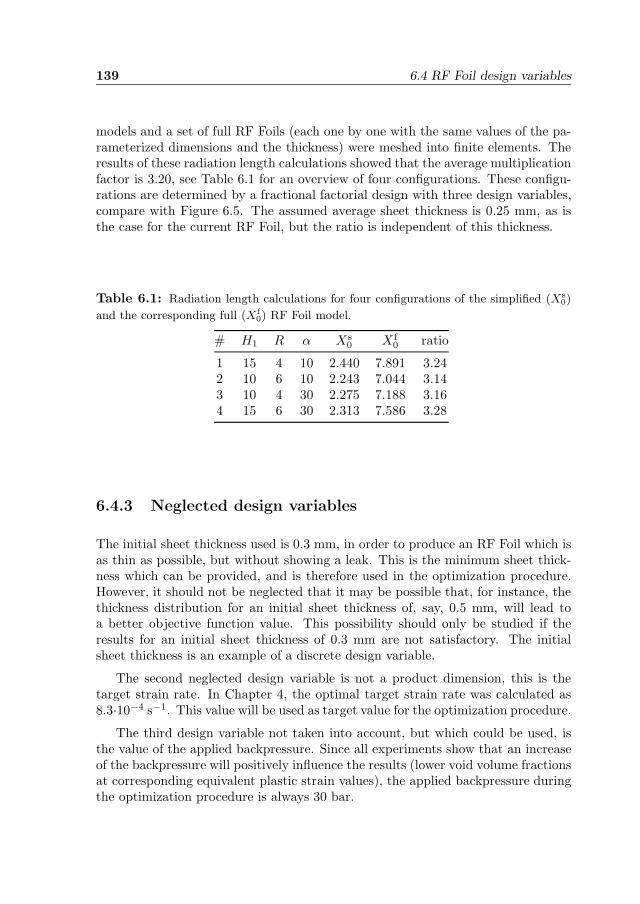
139 6.4 RF Foil design variables
models and a set of full RF Foils (each one by one with the same values of the pa-rameterized dimensions and the thickness) were meshed into finite elements. Theresults of these radiation length calculations showed that the average multiplicationfactor is 3.20, see Table 6.1 for an overview of four configurations. These configu-rations are determined by a fractional factorial design with three design variables,compare with Figure 6.5. The assumed average sheet thickness is 0.25 mm, as isthe case for the current RF Foil, but the ratio is independent of this thickness.
Table 6.1: Radiation length calculations for four configurations of the simplified (Xs0)
and the corresponding full (Xf0) RF Foil model.
# H1 R α Xs0 X f
0 ratio
1 15 4 10 2.440 7.891 3.242 10 6 10 2.243 7.044 3.143 10 4 30 2.275 7.188 3.164 15 6 30 2.313 7.586 3.28
6.4.3 Neglected design variables
The initial sheet thickness used is 0.3 mm, in order to produce an RF Foil which isas thin as possible, but without showing a leak. This is the minimum sheet thick-ness which can be provided, and is therefore used in the optimization procedure.However, it should not be neglected that it may be possible that, for instance, thethickness distribution for an initial sheet thickness of, say, 0.5 mm, will lead toa better objective function value. This possibility should only be studied if theresults for an initial sheet thickness of 0.3 mm are not satisfactory. The initialsheet thickness is an example of a discrete design variable.
The second neglected design variable is not a product dimension, this is thetarget strain rate. In Chapter 4, the optimal target strain rate was calculated as8.3·10−4 s−1. This value will be used as target value for the optimization procedure.
The third design variable not taken into account, but which could be used, isthe value of the applied backpressure. Since all experiments show that an increaseof the backpressure will positively influence the results (lower void volume fractionsat corresponding equivalent plastic strain values), the applied backpressure duringthe optimization procedure is always 30 bar.
6 Optimization of the RF Foil 140
6.5 Constraints on the RF Foil
In Section 1.5, the requirements on the RF Foil were described. In total, fiverequirements were presented which are acting as constraints on the design of theRF Foil. These are the constraints concerning:
• the leak tightness of the formed sheet, as a maximum value of the overall leakrate;
• a sufficient wake field suppression. It was already concluded that this con-straint is incorporated into the dimensioning of the parameterized model, soit will not be discussed again in this section.;
• the maximum displacement as a result of a 2 mbar overpressure;
• the maximum stress as a result of a 6 mbar overpressure;
• the first natural frequency of the RF Foil.
These constraints, and the impact on the design variables, are described in thissection.
6.5.1 Leak rate constraint
The requirement on the current RF Foil is that for an overpressure of 25 mbar He,the maximum allowable value for the leak rate is 1 · 10−8 mbar·l/s. From Equation(4.21), it follows that the leak rate is proportional to the overpressure Δp. All thespecimens formed during the bulge experiments were leak tested at an overpressureof 1 bar He (i.e. atmospheric pressure). The leak rate implementation accordingto Equation (4.22) is referenced to this 1 bar overpressure. This means that themaximum allowable leak rate at 1 bar overpressure is then (1 bar/25 mbar)·1 ·10−8
mbar·l/s = 4 · 10−7 mbar·l/s.The simplified model is about six times smaller than the full RF Foil. This
means that about one sixth of this leak rate is allowable in the simplified versionof the foil. Therefore, the maximum leak rate in the simplified model will beconstrained to 7 ·10−8 mbar·l/s.
6.5.2 Mechanical constraints
Just as with the leak rate and the radiation length, the mechanical constraints alsohave to be translated from the full RF Foil to the simplified model. This has beendone the same way as was carried out with the radiation length calculations. Fora set of dimensions for the parameterized model, calculations have been done onthe simplified model and the full RF Foil model. The material properties used arethose of AA5083 at room temperature, since this is the temperature at operating
141 6.6 Optimization results
conditions. Under this condition, ALNOVI-1 has a Young’s Modulus of 69 GPa andthe density is 2700 kg/m3. The maximum allowable stress in the material beforefailure is 160 MPa. The calculations resulted in factors to be used as multiplicationon the values calculated for the simplified model.
• the displacement is assumed to be the result of elastic deformation, the max-imum allowable displacement is 1 mm. The deformations in both the sim-plified model and the full RF Foil model have been calculated in differentcombinations of the design variable parameters. An average multiplicationfactor of 5.22 is found. This means that the maximum allowable displacementin the simplified model with a 2 mbar pressure acting on it is 0.192 mm.
• The maximum stress in the structure may not exceed the yield limit. Thismeans that in the full RF Foil, an equivalent stress of 160 MPa may not beexceeded. The same procedure has been followed as with the calculation ofthe deformation multiplication factor. This led to an average multiplicationfactor on the stress of 6.0. This means that in the simplified model, the stressmay not exceed 27 MPa under a pressure load of 6 mbar.
• Also, the ratio of the first natural frequencies were calculated between thesimplified and the full RF Foil model. This led to a multiplication factor of0.52, the first natural frequency of the simplified model is almost twice ashigh. The minimum allowable natural frequency of the full RF Foil is 50 Hz.This means that the first natural frequency of the simplified model should beat least 96 Hz.
6.6 Optimization results
The optimization problem now can be formulated as:
• minimization of the objective function, which is the percentual radiationlength;
• minimize this function by finding an optimal combination of seven designvariables: H1, H2, F1, F2, α, L1 and R.
• the optimization problem is subject to four constraints, concerning leak tight-ness after the forming process, elastic deformation caused by overpressure,stress limit caused by overpressure and the first natural frequency.
In this section, the results of the optimization procedure are presented. For thisprocedure, OptForm has been used in the main part. The results of the screeningDesign of Experiments were used to determine the design variables which havethe highest influence on the value of the objective function and/or the constraints.With this information, a Design of Experiments considering the remaining design
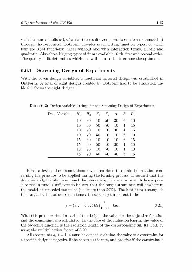
6 Optimization of the RF Foil 142
variables was established, of which the results were used to create a metamodel fitthrough the responses. OptForm provides seven fitting function types, of whichfour are RSM functions: linear without and with interaction terms, elliptic andquadratic. Also three Kriging types of fit are available: 0-th, first and second order.The quality of fit determines which one will be used to determine the optimum.
6.6.1 Screening Design of Experiments
With the seven design variables, a fractional factorial design was established inOptForm. A total of eight designs created by OptForm had to be evaluated, Ta-ble 6.2 shows the eight designs.
Table 6.2: Design variable settings for the Screening Design of Experiments.
Des. Variable H1 H2 F1 F2 α R L1
10 30 10 50 30 6 1010 30 50 50 10 4 1510 70 10 10 30 4 1510 70 50 10 10 6 1015 30 10 10 10 6 1515 30 50 10 30 4 1015 70 10 50 10 4 1015 70 50 50 30 6 15
First, a few of these simulations have been done to obtain information con-cerning the pressure to be applied during the forming process. It seemed that thedimension H2 mainly determined the pressure application in time. A linear pres-sure rise in time is sufficient to be sure that the target strain rate will nowhere inthe model be exceeded too much (i.e. more than 20%). The best fit to accomplishthis target by the pressure p in time t (in seconds) turned out to be
p = (3.2 − 0.025H2)t
1500bar (6.21)
With this pressure rise, for each of the designs the value for the objective functionand the constraints are calculated. In the case of the radiation length, the value ofthe objective function is the radiation length of the corresponding full RF Foil, byusing the multiplication factor of 3.20.
All constraints gi, i = 1..4 must be defined such that the value of a constraint fora specific design is negative if the constraint is met, and positive if the constraint is
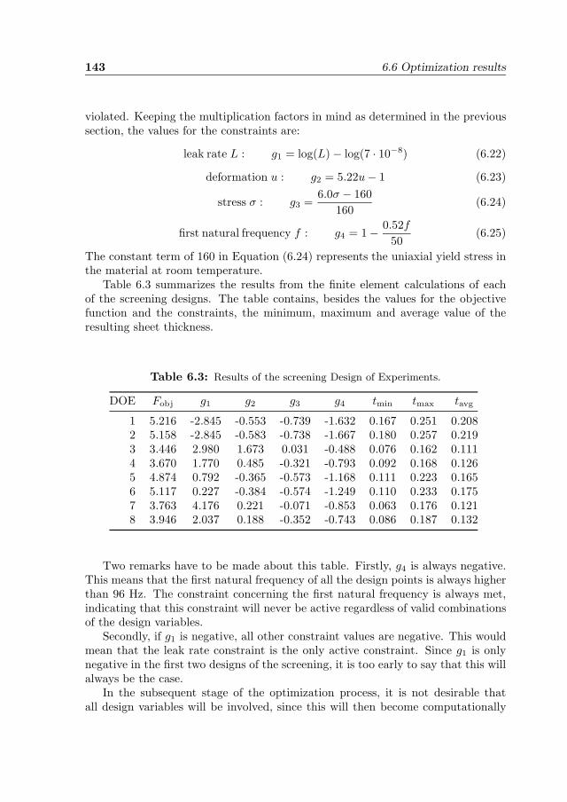
143 6.6 Optimization results
violated. Keeping the multiplication factors in mind as determined in the previoussection, the values for the constraints are:
leak rate L : g1 = log(L) − log(7 · 10−8) (6.22)
deformation u : g2 = 5.22u− 1 (6.23)
stress σ : g3 =6.0σ − 160
160(6.24)
first natural frequency f : g4 = 1 − 0.52f
50(6.25)
The constant term of 160 in Equation (6.24) represents the uniaxial yield stress inthe material at room temperature.
Table 6.3 summarizes the results from the finite element calculations of eachof the screening designs. The table contains, besides the values for the objectivefunction and the constraints, the minimum, maximum and average value of theresulting sheet thickness.
Table 6.3: Results of the screening Design of Experiments.
DOE Fobj g1 g2 g3 g4 tmin tmax tavg
1 5.216 -2.845 -0.553 -0.739 -1.632 0.167 0.251 0.2082 5.158 -2.845 -0.583 -0.738 -1.667 0.180 0.257 0.2193 3.446 2.980 1.673 0.031 -0.488 0.076 0.162 0.1114 3.670 1.770 0.485 -0.321 -0.793 0.092 0.168 0.1265 4.874 0.792 -0.365 -0.573 -1.168 0.111 0.223 0.1656 5.117 0.227 -0.384 -0.574 -1.249 0.110 0.233 0.1757 3.763 4.176 0.221 -0.071 -0.853 0.063 0.176 0.1218 3.946 2.037 0.188 -0.352 -0.743 0.086 0.187 0.132
Two remarks have to be made about this table. Firstly, g4 is always negative.This means that the first natural frequency of all the design points is always higherthan 96 Hz. The constraint concerning the first natural frequency is always met,indicating that this constraint will never be active regardless of valid combinationsof the design variables.
Secondly, if g1 is negative, all other constraint values are negative. This wouldmean that the leak rate constraint is the only active constraint. Since g1 is onlynegative in the first two designs of the screening, it is too early to say that this willalways be the case.
In the subsequent stage of the optimization process, it is not desirable thatall design variables will be involved, since this will then become computationally
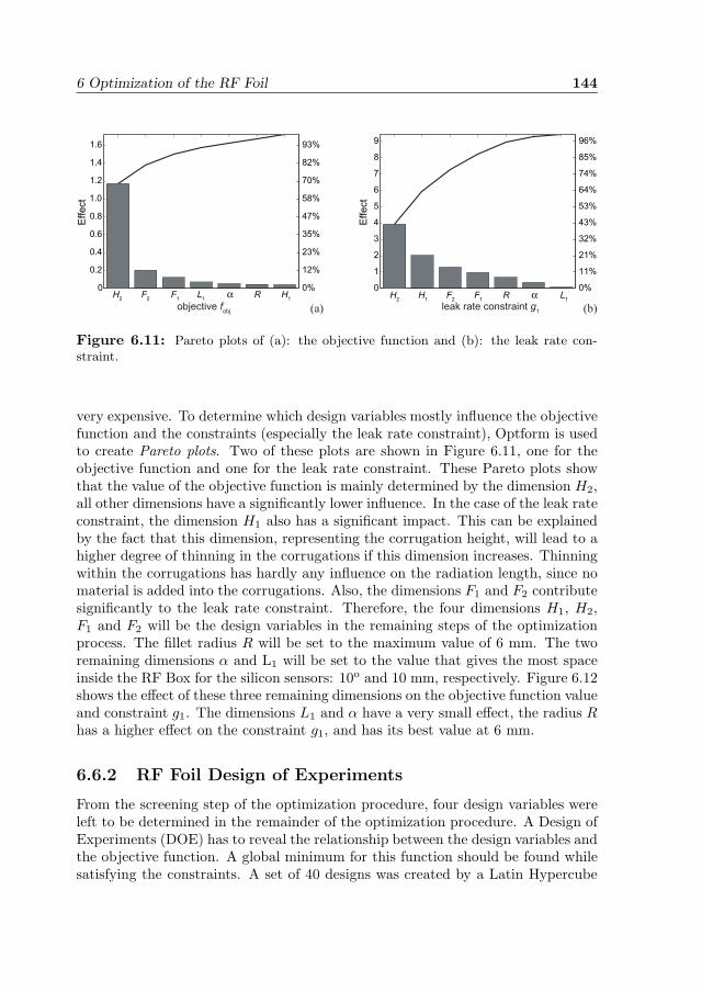
6 Optimization of the RF Foil 144
H2
F2 F
1 L
1 α R H
1
0
0.2
0.4
0.6
0.8
1.0
1.2
1.4
1.6
Effect
0%
12%
23%
35%
47%
58%
70%
82%
93%
H2 H
1 F
2 F
1 R α L
1
0
1
2
3
4
5
6
7
8
9
Effect
0%
11%
21%
32%
43%
53%
64%
74%
85%
96%
objective fobj
leak rate constraint g1(a) (b)
Figure 6.11: Pareto plots of (a): the objective function and (b): the leak rate con-straint.
very expensive. To determine which design variables mostly influence the objectivefunction and the constraints (especially the leak rate constraint), Optform is usedto create Pareto plots. Two of these plots are shown in Figure 6.11, one for theobjective function and one for the leak rate constraint. These Pareto plots showthat the value of the objective function is mainly determined by the dimension H2,all other dimensions have a significantly lower influence. In the case of the leak rateconstraint, the dimension H1 also has a significant impact. This can be explainedby the fact that this dimension, representing the corrugation height, will lead to ahigher degree of thinning in the corrugations if this dimension increases. Thinningwithin the corrugations has hardly any influence on the radiation length, since nomaterial is added into the corrugations. Also, the dimensions F1 and F2 contributesignificantly to the leak rate constraint. Therefore, the four dimensions H1, H2,F1 and F2 will be the design variables in the remaining steps of the optimizationprocess. The fillet radius R will be set to the maximum value of 6 mm. The tworemaining dimensions α and L1 will be set to the value that gives the most spaceinside the RF Box for the silicon sensors: 10o and 10 mm, respectively. Figure 6.12shows the effect of these three remaining dimensions on the objective function valueand constraint g1. The dimensions L1 and α have a very small effect, the radius Rhas a higher effect on the constraint g1, and has its best value at 6 mm.
6.6.2 RF Foil Design of Experiments
From the screening step of the optimization procedure, four design variables wereleft to be determined in the remainder of the optimization procedure. A Design ofExperiments (DOE) has to reveal the relationship between the design variables andthe objective function. A global minimum for this function should be found whilesatisfying the constraints. A set of 40 designs was created by a Latin Hypercube
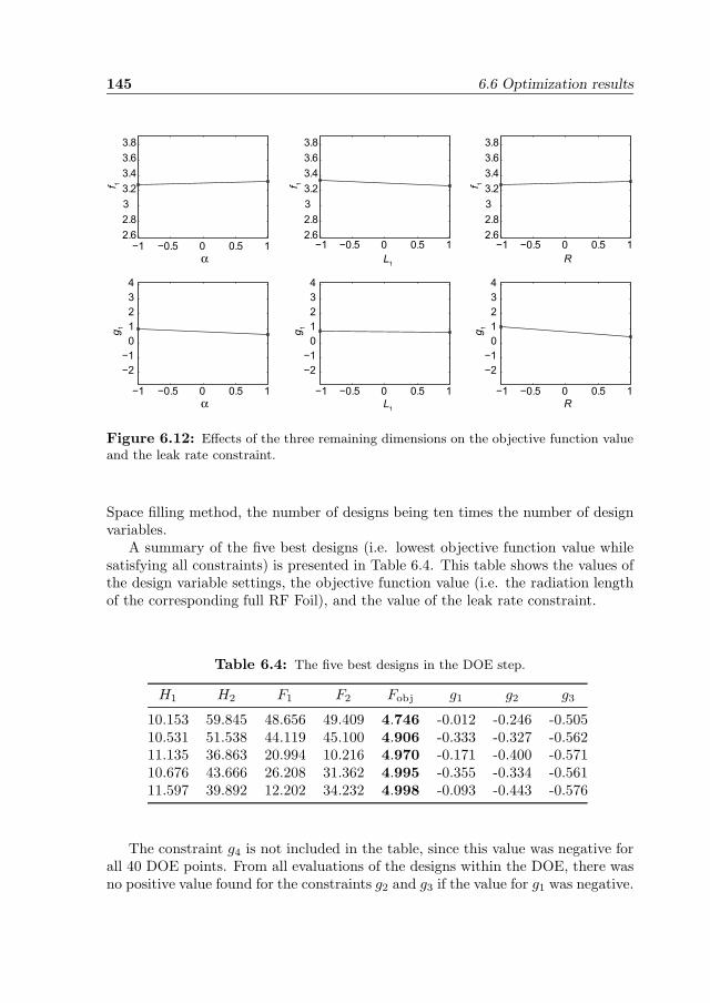
145 6.6 Optimization results
−1 −0.5 0 0.5 12.6
2.8
3
3.2
3.4
3.6
3.8
α
f 1
−1 −0.5 0 0.5 12.6
2.8
3
3.2
3.4
3.6
3.8
L1
f 1
−1 −0.5 0 0.5 12.6
2.8
3
3.2
3.4
3.6
3.8
R
f 1
−1 −0.5 0 0.5 1
−2
−1
0
1
2
3
4
α
g 1
−1 −0.5 0 0.5 1
−2
−1
0
1
2
3
4
L1
g 1
−1 −0.5 0 0.5 1
−2
−1
0
1
2
3
4
R
g 1
Figure 6.12: Effects of the three remaining dimensions on the objective function valueand the leak rate constraint.
Space filling method, the number of designs being ten times the number of designvariables.
A summary of the five best designs (i.e. lowest objective function value whilesatisfying all constraints) is presented in Table 6.4. This table shows the values ofthe design variable settings, the objective function value (i.e. the radiation lengthof the corresponding full RF Foil), and the value of the leak rate constraint.
Table 6.4: The five best designs in the DOE step.
H1 H2 F1 F2 Fobj g1 g2 g3
10.153 59.845 48.656 49.409 4.746 -0.012 -0.246 -0.50510.531 51.538 44.119 45.100 4.906 -0.333 -0.327 -0.56211.135 36.863 20.994 10.216 4.970 -0.171 -0.400 -0.57110.676 43.666 26.208 31.362 4.995 -0.355 -0.334 -0.56111.597 39.892 12.202 34.232 4.998 -0.093 -0.443 -0.576
The constraint g4 is not included in the table, since this value was negative forall 40 DOE points. From all evaluations of the designs within the DOE, there wasno positive value found for the constraints g2 and g3 if the value for g1 was negative.
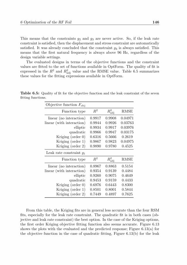
6 Optimization of the RF Foil 146
This means that the constraints g2 and g3 are never active. So, if the leak rateconstraint is satisfied, then the displacement and stress constraint are automaticallysatisfied. It was already concluded that the constraint g4 is always satisfied. Thismeans that the first natural frequency is always above 96 Hz, regardless of thedesign variable settings.
The evaluated designs in terms of the objective functions and the constraintvalues are fitted to the set of functions available in OptForm. The quality of fit isexpressed in the R2 and R2
adj value and the RMSE value. Table 6.5 summarizesthese values for the fitting expressions available in OptForm.
Table 6.5: Quality of fit for the objective function and the leak constraint of the sevenfitting functions.
Objective function Fobj
Function type R2 R2adj RMSE
linear (no interaction) 0.9917 0.9908 0.04971linear (with interaction) 0.9944 0.9926 0.03763
elliptic 0.9934 0.9917 0.03976quadratic 0.9966 0.9947 0.03175
Kriging (order 0) 0.6316 0.5666 0.2619Kriging (order 1) 0.9867 0.9823 0.04975Kriging (order 2) 0.9890 0.9780 0.4525
Leak rate constraint g1
Function type R2 R2adj RMSE
linear (no interaction) 0.8967 0.8863 0.5154linear (with interaction) 0.9354 0.9139 0.4484
elliptic 0.9260 0.9075 0.4649quadratic 0.9453 0.9159 0.4433
Kriging (order 0) 0.6976 0.6443 0.8300Kriging (order 1) 0.8501 0.8001 0.5844Kriging (order 2) 0.7449 0.4897 0.7625
From this table, the Kriging fits are in general less accurate than the four RSMfits, especially for the leak rate constraint. The quadratic fit is in both cases (ob-jective and leak rate constraint) the best option. In the case of the Kriging options,the first order Kriging objective fitting function also seems accurate. Figure 6.13shows the plots with the evaluated and the predicted response; Figure 6.13(a) forthe objective function in the case of quadratic fitting, Figure 6.13(b) for the leak
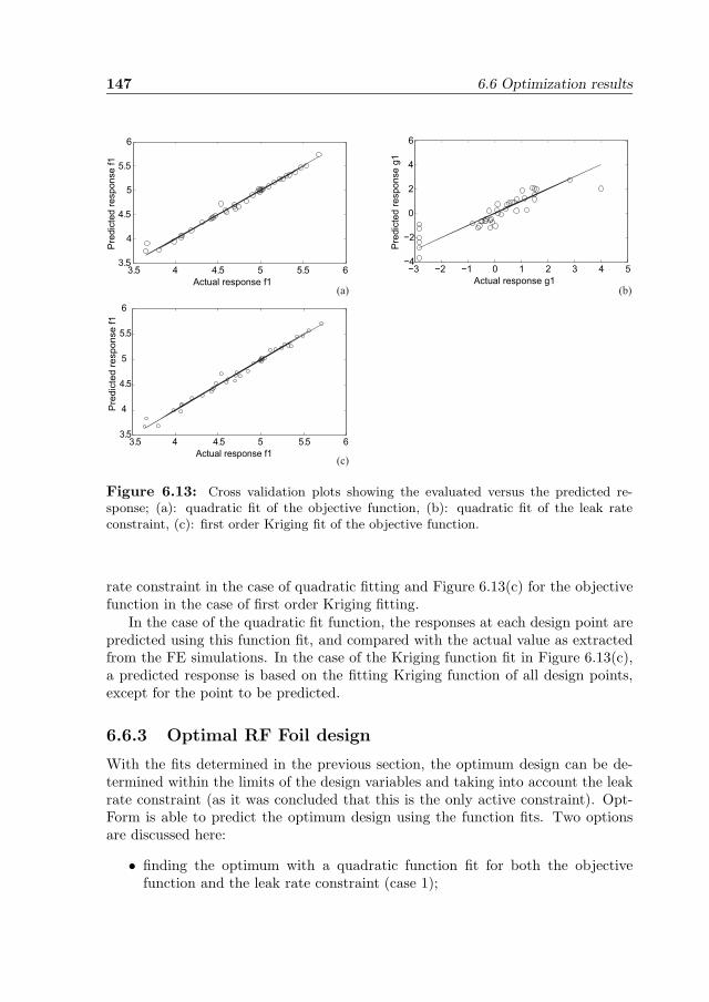
147 6.6 Optimization results
3.5 4 4.5 5 5.5 63.5
4
4.5
5
5.5
6
Actual response f1
Pre
dic
ted r
esponse f1
−3 −2 −1 0 1 2 3 4 5−4
−2
0
2
4
6
Actual response g1
Pre
dic
ted r
esponse g
1
3.5 4 4.5 5 5.5 63.5
4
4.5
5
5.5
6
Actual response f1
Pre
dic
ted
re
sp
on
se
f1
(a)
(c)
(b)
Figure 6.13: Cross validation plots showing the evaluated versus the predicted re-sponse; (a): quadratic fit of the objective function, (b): quadratic fit of the leak rateconstraint, (c): first order Kriging fit of the objective function.
rate constraint in the case of quadratic fitting and Figure 6.13(c) for the objectivefunction in the case of first order Kriging fitting.
In the case of the quadratic fit function, the responses at each design point arepredicted using this function fit, and compared with the actual value as extractedfrom the FE simulations. In the case of the Kriging function fit in Figure 6.13(c),a predicted response is based on the fitting Kriging function of all design points,except for the point to be predicted.
6.6.3 Optimal RF Foil design
With the fits determined in the previous section, the optimum design can be de-termined within the limits of the design variables and taking into account the leakrate constraint (as it was concluded that this is the only active constraint). Opt-Form is able to predict the optimum design using the function fits. Two optionsare discussed here:
• finding the optimum with a quadratic function fit for both the objectivefunction and the leak rate constraint (case 1);
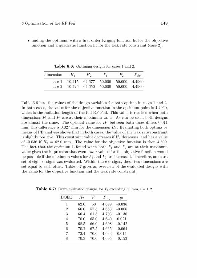
6 Optimization of the RF Foil 148
• finding the optimum with a first order Kriging function fit for the objectivefunction and a quadratic function fit for the leak rate constraint (case 2).
Table 6.6: Optimum designs for cases 1 and 2.
dimension H1 H2 F1 F2 Fobj
case 1 10.415 64.677 50.000 50.000 4.4960case 2 10.426 64.650 50.000 50.000 4.4960
Table 6.6 lists the values of the design variables for both optima in cases 1 and 2.In both cases, the value for the objective function in the optimum point is 4.4960,which is the radiation length of the full RF Foil. This value is reached when bothdimensions F1 and F2 are at their maximum value. As can be seen, both designsare almost the same. The optimal value for H1 between both cases differs 0.011mm, this difference is 0.027 mm for the dimension H2. Evaluating both optima bymeans of FE analyses shows that in both cases, the value of the leak rate constraintis slightly positive. This constraint value decreases if H2 decreases, and has a valueof -0.036 if H2 = 62.0 mm. The value for the objective function is then 4.699.The fact that the optimum is found when both F1 and F2 are at their maximumvalue gives the impression that even lower values for the objective function wouldbe possible if the maximum values for F1 and F2 are increased. Therefore, an extraset of eight designs was evaluated. Within these designs, these two dimensions areset equal to each other. Table 6.7 gives an overview of the evaluated designs withthe value for the objective function and the leak rate constraint.
Table 6.7: Extra evaluated designs for Fi exceeding 50 mm, i = 1, 2.
DOE# H2 Fi Fobj g1
1 62.0 50 4.699 -0.0362 66.0 57.5 4.663 -0.0063 66.4 61.5 4.703 -0.1364 70.0 65.0 4.640 0.0215 68.5 66.0 4.698 -0.1426 70.2 67.5 4.665 -0.0647 72.4 70.0 4.633 0.0148 70.3 70.0 4.695 -0.153
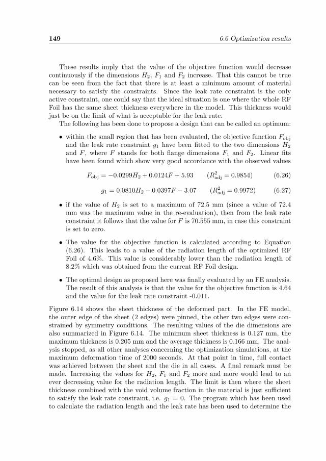
149 6.6 Optimization results
These results imply that the value of the objective function would decreasecontinuously if the dimensions H2, F1 and F2 increase. That this cannot be truecan be seen from the fact that there is at least a minimum amount of materialnecessary to satisfy the constraints. Since the leak rate constraint is the onlyactive constraint, one could say that the ideal situation is one where the whole RFFoil has the same sheet thickness everywhere in the model. This thickness wouldjust be on the limit of what is acceptable for the leak rate.
The following has been done to propose a design that can be called an optimum:
• within the small region that has been evaluated, the objective function Fobj
and the leak rate constraint g1 have been fitted to the two dimensions H2
and F , where F stands for both flange dimensions F1 and F2. Linear fitshave been found which show very good accordance with the observed values
Fobj = −0.0299H2 + 0.0124F + 5.93 (R2adj = 0.9854) (6.26)
g1 = 0.0810H2 − 0.0397F − 3.07 (R2adj = 0.9972) (6.27)
• if the value of H2 is set to a maximum of 72.5 mm (since a value of 72.4mm was the maximum value in the re-evaluation), then from the leak rateconstraint it follows that the value for F is 70.555 mm, in case this constraintis set to zero.
• The value for the objective function is calculated according to Equation(6.26). This leads to a value of the radiation length of the optimized RFFoil of 4.6%. This value is considerably lower than the radiation length of8.2% which was obtained from the current RF Foil design.
• The optimal design as proposed here was finally evaluated by an FE analysis.The result of this analysis is that the value for the objective function is 4.64and the value for the leak rate constraint -0.011.
Figure 6.14 shows the sheet thickness of the deformed part. In the FE model,the outer edge of the sheet (2 edges) were pinned, the other two edges were con-strained by symmetry conditions. The resulting values of the die dimensions arealso summarized in Figure 6.14. The minimum sheet thickness is 0.127 mm, themaximum thickness is 0.205 mm and the average thickness is 0.166 mm. The anal-ysis stopped, as all other analyses concerning the optimization simulations, at themaximum deformation time of 2000 seconds. At that point in time, full contactwas achieved between the sheet and the die in all cases. A final remark must bemade. Increasing the values for H2, F1 and F2 more and more would lead to anever decreasing value for the radiation length. The limit is then where the sheetthickness combined with the void volume fraction in the material is just sufficientto satisfy the leak rate constraint, i.e. g1 = 0. The program which has been usedto calculate the radiation length and the leak rate has been used to determine the
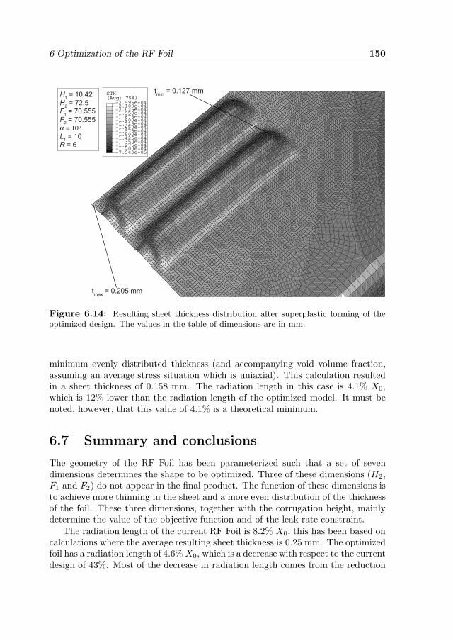
6 Optimization of the RF Foil 150
(Avg: 75%)STH
+1.200e−04+1.275e−04+1.350e−04+1.425e−04+1.500e−04+1.575e−04+1.650e−04+1.725e−04+1.800e−04+1.875e−04+1.950e−04+2.025e−04+2.100e−04
+7.943e−05
+2.996e−04
tmin
= 0.127 mm
tmax
= 0.205 mm
H1 = 10.42
H2 = 72.5
F1 = 70.555
F2 = 70.555
α = 10ο
L1 = 10
R = 6
Figure 6.14: Resulting sheet thickness distribution after superplastic forming of theoptimized design. The values in the table of dimensions are in mm.
minimum evenly distributed thickness (and accompanying void volume fraction,assuming an average stress situation which is uniaxial). This calculation resultedin a sheet thickness of 0.158 mm. The radiation length in this case is 4.1% X0,which is 12% lower than the radiation length of the optimized model. It must benoted, however, that this value of 4.1% is a theoretical minimum.
6.7 Summary and conclusions
The geometry of the RF Foil has been parameterized such that a set of sevendimensions determines the shape to be optimized. Three of these dimensions (H2,F1 and F2) do not appear in the final product. The function of these dimensions isto achieve more thinning in the sheet and a more even distribution of the thicknessof the foil. These three dimensions, together with the corrugation height, mainlydetermine the value of the objective function and of the leak rate constraint.
The radiation length of the current RF Foil is 8.2% X0, this has been based oncalculations where the average resulting sheet thickness is 0.25 mm. The optimizedfoil has a radiation length of 4.6% X0, which is a decrease with respect to the currentdesign of 43%. Most of the decrease in radiation length comes from the reduction

151 6.7 Summary and conclusions
in average sheet thickness, which was reduced from 0.25 to 0.166 mm.From the total set of constraints (leak rate, wake field suppression, mechanical),
the leak rate constraint g1 is the only active constraint. If this constraint is satisfied,then all other constraints are satisfied. The wake field suppression was alreadysatisfied by limiting the corrugation height H1.
Increasing the dimensions H2, F1 and F2 will lead to a decrease in the radiationlength. There is, of course, a limit which is an ideal situation if the sheet were tohave a uniformly distributed thickness. The lower limit on the radiation length isin this case 4.1% X0. The sheet thickness should then be 0.158 mm everywhere inthe model. A radiation length of 4.6% X0 can be called an excellent solution, sincethis is not much higher than the theoretical minimum (13% higher).

6 Optimization of the RF Foil 152
7. Conclusions andrecommendations
This chapter describes the conclusions and recommendations of this research. Thegoal of the project, i.e. reducing the radiation length of the current RF Foil, hasbeen achieved. Three major stages to achieve this goal are distinguished: materialexperiments, material modeling and geometric optimization.
Material experiments Two types of experiments have been performed: tensileexperiments and bulge experiments. The tensile experiments revealed the uniaxialproperties, while the bulge experiments revealed the plane stress properties, theleak rate behavior and the friction between the sheet and the die.
Tensile experiments were performed where two parameters could be influenced:the temperature and the cross head velocity. The temperature was a continuousvariable, the optimal temperature for superplasticity was found to be 520 oC. Atthis temperature, the maximum elongation was reached at all tested drawing ve-locities. This drawing velocity was however not a continuous variable. From thevelocities at which the specimens were tested, an optimal plastic strain rate of8.3·10−4 s−1 was finally found. This would correspond to a drawing velocity of 1.4mm/min.
The bulge experiments were performed by using a dedicated design for thispurpose. The results of these experiments in terms of bulge height were highlyreproducible, due to the program written in LabVIEW to control the temperatureand separate pressures within the experimental setup. During the bulge experi-ments, it was possible to apply a hydrostatic pressure (backpressure) during theforming process. This backpressure had a beneficial effect on the maximum plasticstrain that could be reached and on the leak rate.
Material modeling The uniaxial tests could not be performed with the appli-cation of a backpressure, and at a drawing velocity corresponding to the optimalsuperplastic strain rate for ALNOVI-1. It was, however, possible to develop a ma-terial model which describes the mechanical behavior accurately enough. Since oneof the most important features of the model is the leak rate prediction, and since
153

7 Conclusions and recommendations 154
this leak rate shows a relatively high variance, further refinement would not in-crease the predictability of the leak rate. Therefore, the developed material modelis considered accurate enough to predict the mechanical behavior of ALNOVI-1.
This does not mean that the mechanical behavior is predicted in the mostefficient way. Because of the high strain rate sensitivity, the material behavessomewhere between a solid and a fluid. It was chosen here to use a material modelbased on solid mechanics, which led to satisfactory results.
Geometrical optimization The current geometry of the RF Foil has been pa-rameterized and optimized with respect to radiation length. The optimized proce-dure revealed that the leak rate constraint was the only active constraint. This ledto a design with an average thickness of 0.166 mm. This is well below the averagethickness of the current RF Foil, which means that the optimization procedurewas successful. This is not far above the theoretical value of the minimum averagethickness (with respect to the leak rate) of 0.158 mm.
The goal of this research was to reduce the radiation length of the RF Foil,while making it possible to predict the leak rate of a deformed sheet by numericalanalysis. This goal was achieved by developing a material model which describesthe mechanical behavior including a leak rate prediction in an accurate way. Thismaterial model was used to employ an optimization strategy in order to minimizethe radiation length of the current RF Foil. This radiation length decreased from8.2% X0 to 4.6% X0, the leak rate constraint was met in this case. This is aconsiderable improvement with respect to the current RF Foil.
Other topological solutions may be possible which may lead to even lower ra-diation lengths. If the design will cover most of the view angle as seen from theinteraction point, optimization can be reached in two ways:
• trying to find a procedure which will lead to even lower wall thicknesses with-out introducing leak. In the case of Superplastic Forming, and as mentionedearlier, higher backpressures may be applied, leading to lower void volumefractions at the same equivalent plastic strain values;
• designing a shape such that the average number of crossings through thewalls will be reduced. With the current design, a particle may travel manytimes through the material until a detector is hit. This is especially the casefor particles traveling almost parallel to the beam line. The radiation lengthmay then be decreased by developing a design where these particles will hitfewer walls before hitting a detector.
Recommendations for future work Four recommendations are given herefor future research, in order to investigate whether a further improvement of theradiation length is possible.
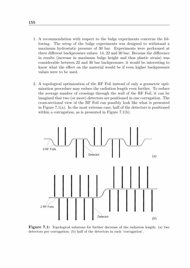
155
1. A recommendation with respect to the bulge experiments concerns the fol-lowing. The setup of the bulge experiments was designed to withstand amaximum hydrostatic pressure of 30 bar. Experiments were performed atthree different backpressure values: 14, 22 and 30 bar. Because the differencein results (increase in maximum bulge height and thus plastic strain) wasconsiderable between 22 and 30 bar backpressure, it would be interesting toknow what the effect on the material would be if even higher backpressurevalues were to be used.
2. A topological optimization of the RF Foil instead of only a geometric opti-mization procedure may reduce the radiation length even further. To reducethe average number of crossings through the wall of the RF Foil, it can beimagined that two (or more) detectors are positioned in one corrugation. Thecross-sectional view of the RF Foil can possibly look like what is presentedin Figure 7.1(a). In the most extreme case, half of the detectors is positionedwithin a corrugation, as is presented in Figure 7.1(b).
Detector
2 RF Foils
Detector
2 RF Foils
(a)
(b)
Figure 7.1: Topological solutions for further decrease of the radiation length: (a) twodetectors per corrugation; (b) half of the detectors in each ’corrugation’.
7 Conclusions and recommendations 156
With this topology, the maximum number of crossings will be decreased sig-nificantly. With this geometry, however, the elastic stiffness decreases withrespect to the current geometry, because the stiffening corrugations have dis-appeared. But since the constraint concerning the elastic stiffness was neveractive, it is worthwhile taking a look at this solution.
3. This research only focused on the manufacturing of the RF Foil by means ofSuperplastic Forming. This forming process is an attractive process, becausethe number of products to be made is very low (2 pieces). Also, the plasticstrains which can be reached are very high and so a large amount of thinningcan be reached. It may be possible to produce these foils in a different manner,by a new method like incremental forming. Especially the latter possibilitycan be investigated in the future as an alternative manufacturing method.
4. A problem with severe thinning in superplastic materials is the growth andcoalescence of voids, and therefore gas leak. The material leaks before itfails in terms of fracture. The question is whether leaks can be mended, forinstance by filling the voids with a secondary material. It is known that themetal gallium can diffuse to voids under certain conditions [80].
A. Control scheme of the bulgeexperiments
A software program was written in LabVIEW to control an entire bulge test. Thisappendix describes the procedure followed by this piece of software, which waswritten at Nikhef. A sheet was positioned inside the experimental setup, on top ofthe Bottom Container. After positioning this setup in the oven and closing the ovendoor, the software program was started. Below is a description of the steps whichwere followed. The abbreviations V1 to V7 correspond with the labels depicted inFigure 3.9.
• When the program starts, the temperature will be constantly monitored whilethe setup heats up. The temperature at which the sheet should be deformedis 520 oC. If the thermocouple readout shows a value of 420 oC, the heaterband injects extra power to the setup to accelerate the temperature rise. Thisheater band is controlled by a PID, which takes care that the target temper-ature will not be exceeded. During this step, V6 ad V7 are opened while allother valves are closed. With V6 open, there will be no pressure differencebetween the Top and Bottom Container. With V7 open, the pressure in theTop and Bottom Container is the same as the atmospheric pressure. If thetarget temperature has been reached, a waiting time of five minutes is appliedto be sure that the whole setup has reached this target temperature.
• The Pressure Bag will be filled with gas until a pressure is reached which is10 bar above the entered backpressure value. This is done by opening andclosing V5. In this way, the aluminum sheet will be clamped on its outerboundary in the stainless steel setup.
• A backpressure will be applied to the Top and Bottom Container by openingV1 and V3. At the beginning of this step, V7 will be closed. To ensure thatno pressure difference will develop between the Top and Bottom Container,V6 stays open.
• The forming pressure is applied by closing V1 and V6 at the beginning ofthis step and by keeping V3 open. Since the forming pressure has to be
157
A Control scheme of the bulge experiments 158
applied very slowly, V3 and V4 work together in order to approximate asclosely as possible the target pressure in time. During the forming process,the volume of the Top Container decreases, because the sheet is deformedupwards. Because the backpressure should not change, V2 is opened to relieveany overpressure.
• If the time limit has been reached, the forming pressure will be released byclosing all valves and then opening V6. This equalizes the pressure betweenthe Top and Bottom Container. This will temporarily increase the backpres-sure a small amount, but this will not affect the outcome of the experiment,since this time span is very small, and there is no forming pressure left. Inthis step, the band heater will be shut off.
• With V6 opened, the backpressure will be released two seconds later, byopening V7. Once atmospheric pressure has been reached, the test is finished.
• A leak detection module has been built inside the program. If, during theforming stage, the sheet should fail by local fracture, then it will becomemore and more difficult to maintain the target forming pressure, since thehole actually takes over the function of an opened valve V6. The backpressurewill increase, so V2 is opened constantly. V3 has to stay opened in order totry to maintain the pressure difference. These two valves are adjusted suchthat a hole in the sheet leads to a non-reversible pressure difference drop, thisdrop will be detected by the program. The software will then stop the testby closing all valves, except V6 and V7.
The pressure in the Pressure Bag has to be released manually after the programstops running. The furnace can then be opened and the formed sheet can be takenout of the Top Container by cooling the sheet with pressurized air. The sheet willdetach from the Top Container since the shrinkage of the sheet is higher due to thehigher thermal expansion coefficient of aluminum with respect to stainless steel.Besides this process, some safety has also been built into the program. If thepressure in one of the pressure vessels exceeds a predefined limit value, then theexperiment is stopped immediately, by opening the valves V6 and V7, and closingall other valves. This will release all the gas which is trapped at that momentin the experiment. In the case of a computer crash or a power failure, all valveswill immediately return to their default, closed, position. Pressures will then notincrease anymore; they have to be released manually.
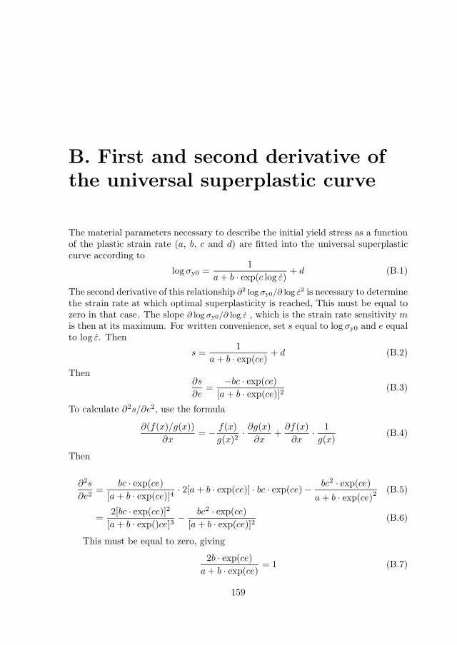
B. First and second derivative ofthe universal superplastic curve
The material parameters necessary to describe the initial yield stress as a functionof the plastic strain rate (a, b, c and d) are fitted into the universal superplasticcurve according to
log σy0 =1
a + b · exp(c log ε)+ d (B.1)
The second derivative of this relationship ∂2 log σy0/∂ log ε2 is necessary to determinethe strain rate at which optimal superplasticity is reached, This must be equal tozero in that case. The slope ∂ log σy0/∂ log ε , which is the strain rate sensitivity mis then at its maximum. For written convenience, set s equal to log σy0 and e equalto log ε. Then
s =1
a + b · exp(ce)+ d (B.2)
Then∂s
∂e=
−bc · exp(ce)[a + b · exp(ce)]2
(B.3)
To calculate ∂2s/∂e2, use the formula
∂(f(x)/g(x))∂x
= − f(x)g(x)2
· ∂g(x)∂x
+∂f(x)
∂x· 1g(x)
(B.4)
Then
∂2s
∂e2=
bc · exp(ce)[a + b · exp(ce)]4
· 2[a + b · exp(ce)] · bc · exp(ce) − bc2 · exp(ce)a + b · exp(ce)2
(B.5)
=2[bc · exp(ce)]2
[a + b · exp()ce]3− bc2 · exp(ce)
[a + b · exp(ce)]2(B.6)
This must be equal to zero, giving
2b · exp(ce)a + b · exp(ce)
= 1 (B.7)
159

B First and second derivative of the universal superplastic curve 160
Working out this equation eventually gives for log ε:
log ε =1c
ln(a
b) (B.8)
By substituting this value in the equation for the first derivative, it is found thatthe strain rate sensitivity m at this point is
mopt =−c
4a(B.9)
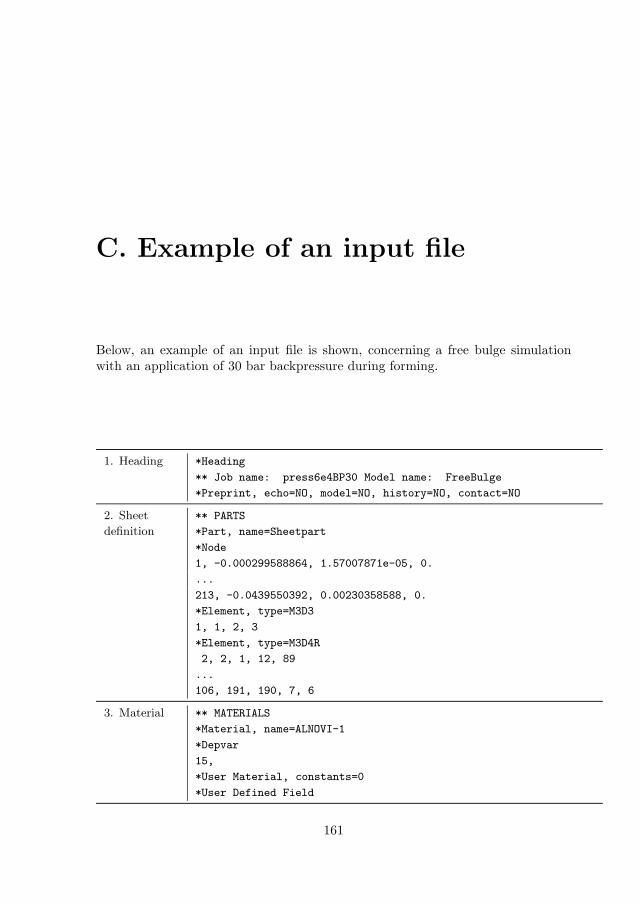
C. Example of an input file
Below, an example of an input file is shown, concerning a free bulge simulationwith an application of 30 bar backpressure during forming.
1. Heading *Heading
** Job name: press6e4BP30 Model name: FreeBulge
*Preprint, echo=NO, model=NO, history=NO, contact=NO
2. Sheet ** PARTS
definition *Part, name=Sheetpart
*Node
1, -0.000299588864, 1.57007871e-05, 0.
...
213, -0.0439550392, 0.00230358588, 0.
*Element, type=M3D3
1, 1, 2, 3
*Element, type=M3D4R
2, 2, 1, 12, 89
...
106, 191, 190, 7, 6
3. Material ** MATERIALS
*Material, name=ALNOVI-1
*Depvar
15,
*User Material, constants=0
*User Defined Field
161
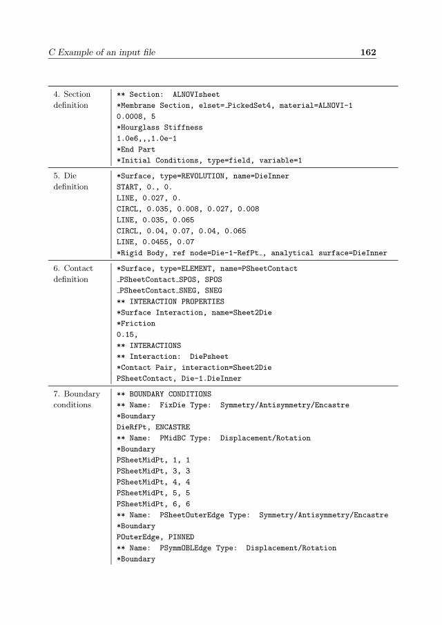
C Example of an input file 162
4. Section ** Section: ALNOVIsheet
definition *Membrane Section, elset= PickedSet4, material=ALNOVI-1
0.0008, 5
*Hourglass Stiffness
1.0e6,,,1.0e-1
*End Part
*Initial Conditions, type=field, variable=1
5. Die *Surface, type=REVOLUTION, name=DieInner
definition START, 0., 0.
LINE, 0.027, 0.
CIRCL, 0.035, 0.008, 0.027, 0.008
LINE, 0.035, 0.065
CIRCL, 0.04, 0.07, 0.04, 0.065
LINE, 0.0455, 0.07
*Rigid Body, ref node=Die-1-RefPt , analytical surface=DieInner
6. Contact *Surface, type=ELEMENT, name=PSheetContact
definition PSheetContact SPOS, SPOS
PSheetContact SNEG, SNEG
** INTERACTION PROPERTIES
*Surface Interaction, name=Sheet2Die
*Friction
0.15,
** INTERACTIONS
** Interaction: DiePsheet
*Contact Pair, interaction=Sheet2Die
PSheetContact, Die-1.DieInner
7. Boundary ** BOUNDARY CONDITIONS
conditions ** Name: FixDie Type: Symmetry/Antisymmetry/Encastre
*Boundary
DieRfPt, ENCASTRE
** Name: PMidBC Type: Displacement/Rotation
*Boundary
PSheetMidPt, 1, 1
PSheetMidPt, 3, 3
PSheetMidPt, 4, 4
PSheetMidPt, 5, 5
PSheetMidPt, 6, 6
** Name: PSheetOuterEdge Type: Symmetry/Antisymmetry/Encastre
*Boundary
POuterEdge, PINNED
** Name: PSymmOBLEdge Type: Displacement/Rotation
*Boundary
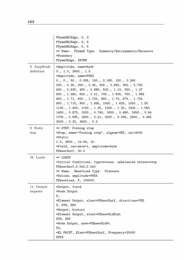
163
PSymmOBLEdge, 3, 3
PSymmOBLEdge, 4, 4
PSymmOBLEdge, 5, 5
** Name: PSymmZ Type: Symmetry/Antisymmetry/Encastre
*Boundary
PSymmZEdge, ZSYMM
8. Amplitude *Amplitude, name=hydr
definition 0., 1.0, 3600., 1.0
*Amplitude, name=P6E4
0., 0., 50., 0.095, 100., 0.165, 150., 0.245
200., 0.35, 250., 0.45, 300., 0.565, 350., 0.705
400., 0.835, 450., 0.985, 500., 1.13, 550., 1.27
600., 1.395, 650., 1.51, 700., 1.605, 750., 1.665
800., 1.71, 825., 1.725, 850., 1.73, 875., 1.725
900., 1.715, 950., 1.685, 1000., 1.625, 1050., 1.55
1100., 1.455, 1150., 1.35, 1200., 1.25, 1300., 1.055
1400., 0.875, 1500., 0.745, 1600., 0.665, 1650., 0.64
1700., 0.585, 1800., 0.51, 2000., 0.435, 2400., 0.365
3000., 0.32, 3600., 0.3
9. Static ** STEP: Forming step
step *Step, name="Forming step", nlgeom=YES, inc=2000
*Static
1.0, 3600., 1e-04, 10.
*Field, variable=1, amplitude=hydr
PSheetSurf, 30.0
10. Loads ** LOADS
*Initial Conditions, type=stress, unbalanced stress=step
PSheetSurf,5.0e3,5.0e3
** Name: SheetLoad Type: Pressure
*Dsload, amplitude=P6E4
PSheetLoad, P, 100000.
11. Output *Output, field
requests *Node Output
U,
*Element Output, elset=PSheetSurf, directions=YES
S, STH, SDV
*Output, history
*Element Output, elset=PSheetMidElmt
STH, SDV
*Node Output, nset=PSheetMidPt
U2,
*EL PRINT, Elset=PSheetSurf, Frequency=20000
SDV9

C Example of an input file 164
1. Model header, including job name and model name.
2. Definition of the sheet geometry in terms of 213 nodes, 106 four-noded quadri-lateral, reduced integration, membrane elements and one three-noded trian-gular membrane element.
3. Material definition, where the user defined material ALNOVI-1 is called.There are 15 state variables defined, the user defined field is meant to definea field where the backpressure can be stored.
4. Section definition: a 0.8 mm thin membrane section with hourglass stiffnesscontrol. The initial conditions are the backpressure values on all the elements.
5. The die is an analytical rigid, which is defined by a set of lines and circleswhich are revolved to obtain a 3-dimensional geometry. A reference point isdefined to which boundary conditions can be applied later.
6. Contact is established by defining contact surfaces. A friction coefficient of0.15 has been applied.
7. The die is fixed in all displacements and rotations. The outer edge of thesheet has been pinned (fixed in all translations). One of the side edges of thesheet has symmetry boundary conditions with respect to the global Z axis.The other side on the edge has symmetry boundary conditions with respectto an oblique, user defined, coordinate system.
8. Two amplitudes must be defined. One is called hydr and is a multiplicationfactor for the hydrostatic pressure. The other amplitude, called P6E4, definesthe forming pressure as a function of time.
9. A static step has been defined, with an initial increment size of 1 second,a maximum increment size of 10 seconds and a minimum increment size of1.0E-4 seconds. The total forming time is 3600 seconds, the backpressure hasbeen set to 30 bar.
10. Before the forming load is applied, an in-plane stress is necessary to preventinitial ill-conditioning due to the fact that membrane elements have beenused. A pressure load of 100000 Pa (= 1 bar), multiplied with the formingpressure amplitude, has been applied.
11. The field output is in terms of the displacements, the stress, the sheet thick-ness and the state variables. The requested history output concerns the dis-placement of the midpoint of the sheet as a function of time. State variable9 (the void volume fraction) has been written, only in the last increment, forall elements to the results file.

Acknowledgments
This chapter provides the only opportunity for me in this thesis to violate somerules that apply to writing scientific reports. Whereas in scientific writing it is notallowed to use personal pronouns like ’I’, ’you’, ’he’ or ’she’, in these three pages, Iwill almost only use them. Also, storytelling is not considered to be scientific, forinstance ’and then ... happened’. However, I am going to tell you a story now.
It all started in the spring of 2004. Then the idea of starting a PhD researchproject came up during a so-called POP meeting (Persoonlijk OntwikkelingsProfielor Personal Development Profile), and it was suggested by the Nikhef HR managerTeus van Egdom. He advised me to discuss the idea with Frank Linde as coor-dinator of the ATLAS project in order to get his opinion and his suggestions forsubjects to study. He supported the idea, and later that year, when Frank becamethe director of Nikhef, he gave me the freedom to choose a subject myself as longas there was a relation with one of the running projects at Nikhef at the time. Intalking to several people, around five topics were suggested. The idea of simulatingthe deformation process of the RF Foil and trying to understand and predict theleak rate of a formed RF Foil came from Rob Klopping and this became the basisof my research project. Frank agreed and on the first day of his directorship hetraveled to the University of Twente in Enschede for a meeting with professor HanHuetink. Han readily agreed to be my supervisor of this PhD research and heappointed a very motivated young staff member of his faculty to be my daily tutorand assistant supervisor, Timo Meinders. Teus, Frank and Rob, thank you verymuch for giving me the opportunity to start this PhD research. Han and Timo,thank you very much for all your support and expertise during the five years thatI spent on the thesis. It has always been a great pleasure to visit you and theuniversity. I particularly enjoyed your ’Twente’ sense of humor and the relaxedatmosphere that goes along with it.
Since Enschede is too far away to work on a daily basis, the home base formy work remained Amsterdam. Bob van Eijk was the supervisor at Nikhef and Ithank you for all the good tips you provided when I needed them. It was also atNikhef where the majority of the mechanical experiments were done. The bulgeexperiments consumed a major part of the five-year period and it was very inspiring
165

ACKNOWLEDGMENTS 166
to experience that our own design of the bulge test setup worked perfectly fine rightfrom the beginning, without any major problems. I said ’our design’ on purposebecause I could not have realized it without the help of Berend Munneke, whohelped with his expertise and who really put a lot of effort in the design. Henot only helped with designing but he was also of great help in the experimentsthemselves, where he spent many hours in assisting and never seemed to be tired topress another series of bulges. Berend, thank you very much for your enthusiasm,contribution and support.
With respect to the bulge experiments, a few more people must be mentioned.The most difficult part of the experimental setup was the manufacturing of thestainless steel pressure vessels which had to be placed inside the furnace. JoopRovekamp did the major part of the manufacturing and I thank you very muchfor your time and patience and for thinking along with regard to certain detailsof the design. Martijn Woldman, a student of Twente University got interestedin Nikhef and my project in particular. He saved me a lot of time by assistingin the experiments. Thank you Martijn for your help. An important part of theexperiments was measuring the leak tightness of the bulges and in order to be ableto do that correctly, they had to be cleaned thoroughly when they came out of theexperiment. And with thoroughly, I really mean thoroughly. With the great helpand experience of Peter Thobe we managed to have all the molecules that had toleave the bulge surface, to leave indeed. Thank you Peter for helping and sharingyour experience.
But before even the bulge experiments could start, the results of the tensileexperiments had to be known. These experiments were done at the University ofGroningen where I got the opportunity to perform the tests at the faculty of Jefde Hosson. He was willing to let me do the tensile tests in one of his labs and heasked two people to help me with the start up: Antony Kazantzis and ZhenguoChen. As real scientists, they did not stop there but also thought along in orderto carry out the experiments in the best way. Jef, Antony and Zhenguo, thankyou very much for offering me your facilities, knowledge and help. And finally, ofcourse, at the very basis of all material experiments, the material itself with whichthe tests are performed is essential. I therefore like to thank Kumi Kawase of thecompany Furukawa Sky Aluminium in Japan for sending me a considerable amountof ALNOVI-1 free of charge.
Then the writing of the PhD thesis itself. This is a constant process of adding,removing and changing text and figures. The comments and suggestions made bythe reading committee proved to be very helpful and led to the draft thesis. BesidesHan and Timo I should thank Jan-Harmen Wiebenga for the critical review on thechapters I wrote. I would also like to thank Semih Perdahcıoglu for reading Chapter4, and Marcel Merk for the remarks on the physics side of the thesis (Chapter 1).Finally, thanks to Vivien Cook for proofreading all chapters (except this one!) andreviewing the thesis on English spelling and grammar. The draft thesis could then

167 ACKNOWLEDGMENTS
be turned into the final thesis, of which this book is proof. It was finalized thanksto some last, extra remarks of the examiners. Besides the people I already thankedfor all their help, I would also like to thank Richard Wood from Swansea Universityin Wales and Remko Akkerman in this context, for their willingness to take placein the examination committee.
And now it is time to change to Dutch.Behalve de inhoudelijke en administratieve hulp, is er ook heel veel steun en inter-esse geweest van familie en vrienden. In die twee termen zit overigens een groteoverlap. Om de familie en een groot deel van de vriendenkring te noemen, maak ikgebruik van de term ’grootfamilie’ waarin iedereen zit die zich aangesproken voeltdoor de achternaam Snippe, van der Veen, Moens, Hammecher, Hooman, Bessel-ing, Berendsen, Streppel en Ribeiro. Allen hebben zeer grote interesse getoondin hetgeen ik deed, en een veelgehoorde vraag was of ik het nog een keer wildeuitleggen. Dat deed ik graag.
Maar ik wil er natuurlijk een aantal mensen uitlichten. Ten eerste wil ik mijnzus Solveg en haar vriend Rene bedanken voor de gastvrijheid en gezelligheid dieik genoten heb in de tijd dat ik materiaalexperimenten deed op de universiteit vanGroningen. Natuurlijk hebben we elkaar in die vijf jaar veel vaker gezien, maarjullie huis was een geweldige plek om te verblijven in die periodes.
Vele anderen hielpen bij het verzetten van de zinnen door nachtelijke drink-en spelletjessessies op geregelde tijden (Tineke en Willem, Bas en Carlos). Zinnenwerden ook verzet door het spelen van muziek, dit heeft een extra impuls gekregentoen ik als basgitarist werd opgenomen in de band die, tijdens het ter perse gaanvan dit proefschrift, nog steeds naamloos door het leven gaat.
Lest best Vier mensen wil ik graag onder dit kopje scharen, twee daarvan zijnal eerder genoemd. Aangezien zij naast alle hulp en interesse de zware taak vanparanimf op zich hebben willen nemen, mogen ze nog een keer genoemd: BerendMunneke en Carlos Ribeiro, dank jullie wel voor het willen vervullen van deze taak!Eerder heb ik al de mensen genoemd zonder wie ik nooit aan een promotie hadkunnen werken, maar er missen er nog twee: mijn vriendin Dorien en onze zoonJasper. Dankzij hun begrip en medewerking heb ik de vele extra uren die ik aanmijn promotie heb moeten besteden ook zonder probleem kunnen besteden. Ik hebvan hen veel interesse en steun mogen ervaren en Dorien heeft door de jaren heenook veel geholpen met het corrigeren van mijn teksten in het Engels en is mededaardoor ook aardig op de hoogte van de hoofdlijnen van mijn onderzoek. Allebeisuperveel bedankt en een dikke kus!

ACKNOWLEDGMENTS 168

Bibliography
[1] J. Arora. Introduction to Optimum Design. Elsevier Academic Press, 2ndedition, 2004.
[2] M. Ashby and R. Verrall. Diffusion-accommodated flow and superplasticity.Acta Metallurgica, 21:149–163, 1973.
[3] D. Bae and A. Ghosh. Grain size and temperature dependence of superplasticdeformation in an Al-Mg alloy under isostructural condition. Acta Materialia,48:1207–1228, 2000.
[4] D. Bae and A. Ghosh. Cavity growth during superplastic flow in an Al-Mgalloy: I. Experimental study. Acta Materialia, 50:993–1009, 2002.
[5] D. Bae and A. Ghosh. Cavity growth in a superplastic Al-Mg alloy: II. Animproved plasticity based model. Acta Materialia, 50:1011–29, 2002.
[6] N. v. Bakel. The silicon vertex detector for LHCb: interaction with the LHCbeams and the design of a radiation hard front-end chip. PhD thesis, VrijeUniversiteit Amsterdam, 2004.
[7] N. v. Bakel, J. v. d. Brand, and M. Ferro-Luzzi. A first study of wake fieldsin the LHCb vertex detector. Technical report, NIKHEF, 1999. LHCb note99-041/VELO.
[8] N. v. Bakel, J. v. d. Brand, and M. Ferro-Luzzi. Wake fields in the LHCbvertex detector: alternative designs for the wake field suppressor. Technicalreport, VU Amsterdam, 1999. lhcb-99-044.
[9] F. Barlat, J. Brem, J. Yoon, K. Chung, D. R.E., D. Lege, S.-H. Pourboghrat,and E. Choi. Plane stress yield function for aluminum alloy sheets - part 1:theory. International Journal of Plasticity, 19:1297–1319, 2003.
[10] J. Bonet, A. Gil, R. Wood, R. Said, and R. Curtis. Simulating superplasticforming. Computer Methods in Applied Mechanics and Engineering, 195:6580–603, 2006.
169
BIBLIOGRAPHY 170
[11] M. Bonte. Optimisation Strategies for Metal Forming Processes. PhD thesis,Twente University, 2007.
[12] A. v. d. Boogaard. Thermally Enhanced Forming of Aluminium Sheets: Mod-elling and Experiments. PhD thesis, Twente University, 2002.
[13] L. Carrino, G. Giuliano, and N. Ucciardello. Analysis of void growth in super-plastic materials. Journal of Materials Processing Technology, 155:1273–1279,2004.
[14] CERN. LHCb VeLo Technical Design Report. Technical Report 2001-011,CERN, 2001.
[15] N. Chandra. Constitutive behavior of superplastic materials. Intl. Journal ofNon-Linear Mechanics, 37:461–484, 2002.
[16] Y. Chen, K. Kibble, R. Hall, and X. Huang. Numerical analysis of superplasticblow forming of Ti-6Al-4V alloys. Materials and Design, 22:679–685, 2001.
[17] Z. Chen and T. P.F. A study of post-form static and fatigue properties ofsuperplastic 7475-SPF and 5083-SPF aluminium alloys. Journal of MaterialsProcessing Technology, 148:204–219, 2004.
[18] Z. Chen and P. Thomson. Friction against superplastic aluminium alloys.Wear, 201:227–232, 1996.
[19] A. Chezan and J. De Hosson. Superplastic behavior of coarse-grained alu-minum alloys. Materials Science and Engineering A, 410-411:120–123, 2005.
[20] A. Chokshi and A. Mukherjee. The influence of hydrostatic pressure on grainboundary sliding in superplasticity: implications for cavitation. MaterialsScience and Engineering A, 171:47–54, 1993.
[21] R. Cleveland, A. Ghosh, and J. Bradley. Comparison of superplastic behaviorin two 5083 aluminum alloys. Materials Science and Engineering A, 351:228–236, 2003.
[22] G. Cornfield and R. Johnson. The forming of superplastic sheet metal. Inter-national Journal of Mechanical Sciences, 12:479–490, 1970.
[23] T. Courtney. Mechanical Behavior of Materials. Mc Graw-Hill, 1990.
[24] F. Dunne and N. Petrinic. Introduction to Computational Plasticity. OXFORDUniversity Press, 2005.
[25] Furukawa Sky Aluminium Ltd. Superplastic 5083 aluminium alloy sheetALNOVI-1 was approved by airbus. Furukawa Review 26, 2004.
171 BIBLIOGRAPHY
[26] F. Giordano, A. Natale, and M. Calvagni. Numerical Simulation of the SuperPlastic Forming Process of the EFA - 2000 Under Carriage Door. TechnicalReport 2001-117, Alenia Aerospazio, 2001.
[27] D. Groom et al. Particle physics booklet. Springer, Particle Data Group, 2000.
[28] J. Hedworth and M. Stowell. The Measurement of Strain-Rate Sensitivity inSuperplastic Alloys. Journal of Materials Science, 6:1061–1069, 1971.
[29] R. Hierck. Optimisation of the LHCb detector. PhD thesis, Vrije UniversiteitAmsterdam, 2003.
[30] R. Hino, A. Sasaki, F. Yoshida, and V. Totopov. A new algorithm for reduc-tion of number of press-forming stages in forging processes using numericaloptimization and fe simulation. International Journal of Mechanical Sciences,50:974–983, 2008.
[31] M. Hojjati, M. Zoorabadi, and S. Hosseinipour. Optimization of superplastichydroforming process of aluminium alloy 5083. Journal of Materials ProcessingTechnology, 205:482–488, 2008.
[32] W. Hosford. Yield locus of randomly oriented fcc metals according to theBishop-Hill theory. Metallurgical Transactions, 4:1416–1417, 1973.
[33] W. Hosford. Comments on anisotropic yield criteria. International Journal ofMechanical Sciences, 27:423–427, 1985.
[34] J. Huetink et al. Mechanics of Forming Processes. Graduate School Engineer-ing Mechanics, 2003.
[35] J. Huetink and T. Meinders. Solid Mechanics II: Plasticity. Universiteit-Twente, 2005.
[36] M. Jain, M. Chaturvedi, N. Richards, and N. Goel. Strain rate sensitivityeffects with forming characteristics of superplastic Ti6Al4V. Materials Scienceand Engineering A, 138(2):205–211, 1991.
[37] O. Kaibyshev. Fundamental aspects of superplastic deformation. MaterialsScience and Engineering A, 324:96–102, 2002.
[38] F. v. Keulen, R. Haftka, and N. Kim. Review of options for structural designsensitivity analysis. part 1: Linear systems. Computer Methods in AppliesMechanics and Engineering, 194:3213–3243, 2005.
[39] M. Khaleel, H. Zbib, and E. Nyberg. Constitutive modeling of deformationand damage in superplastic materials. Intl. Journal of Plasticity, 17:277–296,2001.
BIBLIOGRAPHY 172
[40] M. Kraan. http://www.nikhef.nl/pub/departments/mt/projects/lhcb-vertex/.Nikhef, 2010.
[41] G. Krallics and J. Lenard. An examination of the accumulative roll-bondingprocess. Journal of Materials Processing Technology, 152(2):154–161, 2004.
[42] M. Lagos and H. Luque. Two-phase theory for the superplastic flow. Interna-tional Journal of Plasticity, 17:369–386, 2001.
[43] T. Langdon. The mechanical properties of superplastic material. Metallurgicaland Materials Transactions A, 13(5):689–701, 1982.
[44] T. Langdon. Creep at low stresses: an evaluation of diffusion creep and Harper-Dorn creep as viable creep mechanisms. Metallurgical and Materials Transac-tions A, 33:249–259, 2002.
[45] D. Lassance, F. Scheyvaerts, and T. Pardoen. Growth and coalescenceof penny-shaped voids in metallic alloys. Engineering Fracture Mechanics,73:1009–1034, 2006.
[46] H. Lee, J. Yoon, C. Park, Y. Ko, D. Shin, and C. Lee. A study on diffusionbonding of superplastic Ti-6Al-4V ELI grade. Journal of Materials ProcessingTechnology, 187-188:526–529, 2007.
[47] S. Lee, J. Yoon, and D. Yang. A stress integration algorithm for plane stresselastoplasticity and its applications to explicit finite element analysis of sheetmetal forming processes. Computers & Structures, 66:301–311, 1998.
[48] G. Li, M. Tan, and K. Liew. Three-dimensional modeling and simulation ofsuperplastic forming. Journal of Materials Processing Technology, 150:76–83,2004.
[49] J. Libby and T. Ruf. The material distribution in a realistic VELO design.Technical report, CERN, 2001. LHCb 2001-019 VELO.
[50] J. Lin and T. Dean. Modelling of microstructure evolution in hot forming usingunified constitutive equations. Journal of Materials Processing Technology,167:354–362, 2005.
[51] S. Luckey Jr., P. Friedman, and K. Weinmann. Correlation of finite elementanalysis to superplastic forming experiments. Journal of Materials ProcessingTechnology, 194:30–37, 2007.
[52] J. MacFarlane. VISRAD- a 3-D view factor code and design tool for high-energy density physics experiments. Journal of Quantitative Spectroscopy &Radiative Transfer, 81:287–300, 2003.

173 BIBLIOGRAPHY
[53] R. Mahidhara and A. Mukherjee. Mechanisms of cavity growth in a fine-grained 7475 al superplastic alloy. Materials and Design, 16(6):343–348, 1995.
[54] K. Mattiasson and M. Sigvant. An evaluation of some recent yield criteriafor industrial simulations of sheet forming processes. International Journal ofMechanical Sciences, 2007.
[55] M. Meier. The Hall-Petch relationship. Department of Chemical Engineeringand Materials Science, University of California, Davis, September 2004.
[56] F. Mohamed. The role of boundaries during superplastic deformaton. Surfaceand Interface Analysis, 31:532–546, 2001.
[57] F. Mohamed. The role of impurities during creep and superplasticity at verylow stresses. Metallurgical and Materials Transactions A, 33(2):261–278, 2002.
[58] R. Myers and D. Montgomery. Response Surface Methodology: Process andProduct Optimization Using Designed Experiments. Wiley, 2nd edition, 2002.
[59] T. Naka, Y. Nakayama, T. Uemori, R. Hino, and F. Yoshida. Effects on tem-perature on yield locus for 5083 aluminium alloy sheet. Journal of MaterialsProcessing Technology, 140:494–499, 2003.
[60] A. Needleman. An analysis of ductile rupture in notched bars. J. Mech. Phys.Solids, 32(6):461–490, 1984.
[61] K. Padmanabhan. On the evaluation of the activation energy for superplasticflow. Journal of Materials Science, 16(2):531–533, 1981.
[62] K. Padmanabhan, R. Vasin, and F. Enikeev. Superplastic Flow: Phenomenol-ogy and Mechanics. Springer, 2001.
[63] R. Peerlings. Plasticity of porous materials. EM Graduate Course Microme-chanics, Ch11, 2004.
[64] J. Pilling. Superplasticity in Crystalline Solids, from http://home.comcast.net/∼brandihampson/sp/index.html. Technical report, Michigan Technologi-cal University.
[65] J. Pilling, N. Ridley, and M. Islam. On the modelling of diffusion bonding inmaterials: superplastic super alpha-2. Materials Science and Engineering A,205:72–78, 1996.
[66] A. Pye. Superplastic forming of aluminium alloys. Materials & Design,2(6):304–309, 1981.
BIBLIOGRAPHY 174
[67] N. Queipo, R. Haftka, W. Shyy, T. Goel, R. Vaidyanathan, and P. Tucker.Surrogate-based analysis and optimization. Progress in Aerospace Sciences,41:1–28, 2005.
[68] A. Ragab. Modeling the effect of cavitation on tensile failure of superplasticalloys. Materials Science and Engineering A, 454-455:614–622, 2007.
[69] N. Ridley, P. Bate, and B. Zhang. Material modelling data for superplas-tic forming optimisation. Materials Science and Engineering A, 410:100–104,2005.
[70] S. Semiatin, V. Seetharaman, et al. Cavitation during hot tension testing ofTi-6Al-4V. Materials Science and Engineering A, 256:92–110, 1998.
[71] V. Senthil Kumar, D. Viswanathan, and S. Natarajan. Theoretical predictionand FEM analysis of superplastic forming of AA7475 aluminium alloy in ahemispherical die. Journal of Materials Processing Technology, 173:247–251,2006.
[72] J. Simo and T. Hughes. Computational Inelasticity. Springer-Verlag, 1998.
[73] Simulia. ABAQUS Analysis User’s Manual. 2007.
[74] Simulia. ABAQUS Theory Manual. 2007.
[75] Simulia. ABAQUS User Subroutines and Parametric Studies. 2007.
[76] W. Soer, A. Chezan, and J. De Hosson. Deformation and reconstruction mech-anisms in coarse-grained superplastic almg alloys. Acta Materialia, 54:3827–3833, 2006.
[77] W. Swann. A survey of non-linear optimization techniques. FEBS Letters,2:S39–S55, 1969.
[78] C. Syn, M. O’Brien, D. Lesuer, and O. Sherby. An Analysis of Gas PressureForming of Superplastic AL 5083 Alloy. LIMAT-2001 Int’l Conference onLight Materials for Transportations Systems, (UCRL-JC-135190), May 2001.
[79] D. Tabor. Gases, liquids and solids. Cambridge, 2nd edition, 1985.
[80] W. Tsai, Y. Hwu, C. Chen, L. Chang, J. Je, H. Lin, and G. Margaritondo.Grain boundary imaging, gallium diffusion and the fracture behavior of Al-Zn Alloy - An in situ study. Nuclear Instruments and Methods in PhysicsResearch B, 199:457–463, 2003.
[81] R. Valiev and O. Kaibyshev. On the quantitative evaluation of superplasticflow mechanisms. Acta Metallurgica, 31(12):2121–2128, 1983.
175 BIBLIOGRAPHY
[82] R. Vasin, F. Enikeev, M. Mazurski, and O. Munirova. Mechanical modelling ofthe universal superplastic curve. Journal of Materials Science, 35:2455–2466,2000.
[83] R. Verma, A. Ghosh, S. Kim, and C. Kim. Grain refinement and superplas-ticity in 5083 Al. Materials Science and Engineering A, 191:143–150, 1995.
[84] W. Williams. Nuclear and Particle Physics. Oxford Science Publications,1997.
[85] H. Xing, C. Wang, et al. Recent developments in the mechanics of super-plasticity and its applications. Journal of Materials Processing Technology,151:196–202, 2004.
[86] J. Yoon, F. Barlat, R. Dick, K. Chung, and T. Kang. Plane stress yield functionfor aluminum alloy sheets - Part II: FE formulation and its implementation.International Journal of Plasticity, 20:495–522, 2004.
[87] J. Yoon, D. Yang, and K. Chung. Elasto-plastic finite element method basedon incremental deformation theory and continuum based shell elements forplanar anisotropic sheet materials. Comput. Methods Appl. Mech. Engrg.,174:23–56, 1999.
[88] H. Young and R. Freedman. University Physics. Addison Wesley, 9th edition,1996.