Design and Implementation of Soil Loss System Based on RUSLE

Design and Implementation of Soil Loss System Based on RUSLE

CHEN JINXING, YUE DEPENG*, SHANG SHU, MA MENGCHAO

Institute of GIS，RS ＆ GPS ,School of Forestry

Beijing Forestry University

Tsinghua East Road No. 35, Beijing, 100083, China

Email:[email protected]

Abstract:Soil erosion is a serious hazard that causes damages to environment and causes other problems. To

compute soil loss, a system that merges with geographic information system(gis) is developed. This program

uses the model of Revised Universal Soil Loss Equation (RUSLE).It is built on Microsoft.NET Framework 4,

combined with integrated secondary development tool ArcGIS Engnie 10.1.This program can compute the six

RUSLE factors, namely rainfall erosivityfactor,vegetation cover management factor, soil erodibility factor,

slope length factor, slope angle factor and conservation practice factor by inputting corresponding layers. The

system provides visualization interface and it is easy to use .We use the data of Beijing as an example for

application. The spatial distribution map of soil erosion is generated and it is classified into five levels, which

can monitor the distribution of soil erosion patterns. The results are in line with the soil erosion tendency. The

soil erosion map will facilitate the allocation of conservation resources and the enacting of relative regulations.

Key words:soil erosion, RUSLE, interpolation, slope length, ArcGIS Engnie, NDVI

1 Introduction

Soil erosion and degradation of land resources are

significant problems in a large number of

countries[1].It not only causes damage to cultivated

soils, but also affects water quality and is responsible

for sediment transport, causing many remote

problems such as mud floods[2]. Therefore, an

effective way of calculating soil erosion amount can

facilitate relevant management. There exist many

models and programs predicting and calculating soil

losses such as European soil Erosion

Models,EUROSEM/KINEROS,ANSWERS and

CREAMS. However, some of these models are too

sophisticated to use, some lack of sufficient

verification and some need data that are hard to

obtain. Fortunately, the Universal Soil Loss Equation,

simple and easy to use, has been extensively used all

over the world since it was developed by Wischmeier

and Smith in 1956.This equation was put forward

according to statistical analysis of erosion data from

a large number of plot studies under different

conditions[3]. Revised Universal Soil Loss Equation

(RUSLE) and modified Universal Soil Loss Equation

(MUSLE) has improved the algorithm and expanded

its application scopes.

Though some programs applicating the Universal

Soil Loss Equation has been developed, in case of

The Universal Soil loss Equation Computer Program

developed by Wisconsin-Madison[4] which requires

strict data forms and is difficult to manipulate.

Geographic information system has been integrated

with RUSLE to evaluate soil erosion. Many

commercial GIS products such as ArcGIS Desktop

and SuperMapDeskpro have been used in many

studies. Nevertheless, their applications are limited

for high cost, complex installation, too large memory

space and other factors[5].Due to these problems, we

develop a Soil Loss System based on revised

Universal Soil Loss Equation.

This program can display results as maps with

many pixels showing its spatial

distribution.In consideration of the applicability in

different regions and scales, easy acquisition

methods are used in the calculation of each factor.

RUSLE is integrated into the program and it use the

digitized data estimate soil erosion amount. It has

light graphic user interface and geographical spatial

data is easily utilized and in contact with users with

different professional knowledge. Spatial query is

realized by inputting corresponding search criteria.

WSEAS TRANSACTIONS on INFORMATION SCIENCE and APPLICATIONSChen Jinxing, Yue Depeng, Shang Shu, Ma Mengchao

E-ISSN: 2224-3402 204 Volume 11, 2014

Data management、data browse and results output are

also implemented in this program. User can wander

in the soil loss region and zoom in and out the

region.

2 System Design and development

2.1 System structure

The development of this program is built on

Microsoft.NET Framework 4. C# was used to

create the program under the platform of

Microsoft Visual studio 2010 by embedding

ArcGIS Engnie 10.1. And Microsoft.NET

Framework 4 is a technology that supports

building and running the generation of

applications and XML Web services. C♯ is a

simple object-oriented programming language

which can improve the efficiency of system

development. ESRI issued ArcGIS Engine 10.1

in 2012 which is the component of the packaged

ArcObjects. ArcGIS Engine contains GIS

components that allows developers to build

custom mapping applications. It is convenient to

develop applications by using ArcGIS Engnie

which saves time and cost. The programs

developed by ArcGIS Engine can run on client

computer after installing ArcGIS Engine

Runtime. Our program can be installed on

windows 8/7/xp. It requires Microsoft.NET

Framework 4 except for windows 8 which has

already got .NET Framework 4.

This system mainly consists of seven functions

including rainfall calculation, slope length

calculation, slope calculation, soil erodibility

acquisition, cover and management practices factor

calculation, support practice calculation and statistics,

as is shown in figure 1. System includes data layer,

plug-in layer and application layer. Personal

Geodatabase spatial data model is used in the

program and ArcSDE spatial data engine is used to

manage spatial data and attribute data in data layer

including raster data, vector data and tables. Plug-in

layer links the data in the database with user,

including data storage and data reading. Application

layer interacts with user and it can implicate basic

functions, render map, calculate soil loss and query

spatial data.

Fig. 1 The system architecture

2.2 Soil Erosion Model

Types of erosion generally take place in varied stages

of an erosion process, including raindrop erosion,

gully erosion, the deposition of soil particles and so

on[6].RUSLE considers these processes and the

factors that affect soil loss, which is expressed in the

following:

(1) P*C*S*L*K*RA =

A is annual soil loss (t ha-1

·a-1

); R is rainfall

erosivity factor (MJ mm ha-1

h1·a-1

); K is soil

erodibility factor (t ha-1

MJ-1

mm-1); L, S, C,P are

dimensionless factors respectively representing slope

length, slope angle, vegetation cover and

management practices and supporting practices

[7][8].

The data required by R includes rainfall records,

DEM,NDVI, soil map, land use map as is shown in

figure 2.After interpolation, rainfall of the region’s

envelop is produced, then mask it with the research

area’s extent and C factor will be created.

Topographic factors, slope angle and slope length,

are calculated from DEM by several steps.NDVI is

adopted to create C factor. Soil map and land use

map are vector maps which will be converted to

raster maps. At last multiply the six factors and the

soil loss map is created.


E-ISSN: 2224-3402 205 Volume 11, 2014

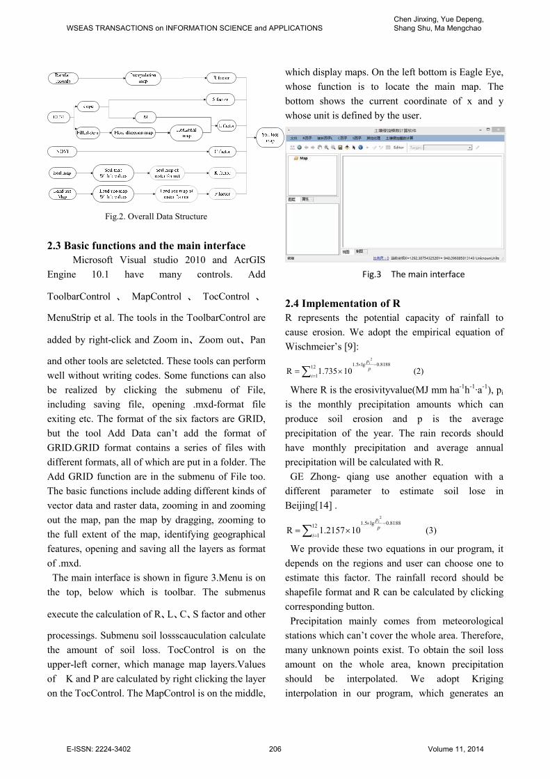
Fig.2. Overall Data Structure

2.3 Basic functions and the main interface

Microsoft Visual studio 2010 and AcrGIS

Engine 10.1 have many controls. Add

ToolbarControl 、 MapControl 、 TocControl 、

MenuStrip et al. The tools in the ToolbarControl are

added by right-click and Zoom in、Zoom out、Pan

and other tools are seletcted. These tools can perform

well without writing codes. Some functions can also

be realized by clicking the submenu of File,

including saving file, opening .mxd-format file

exiting etc. The format of the six factors are GRID,

but the tool Add Data can’t add the format of

GRID.GRID format contains a series of files with

different formats, all of which are put in a folder. The

Add GRID function are in the submenu of File too.

The basic functions include adding different kinds of

vector data and raster data, zooming in and zooming

out the map, pan the map by dragging, zooming to

the full extent of the map, identifying geographical

features, opening and saving all the layers as format

of .mxd.

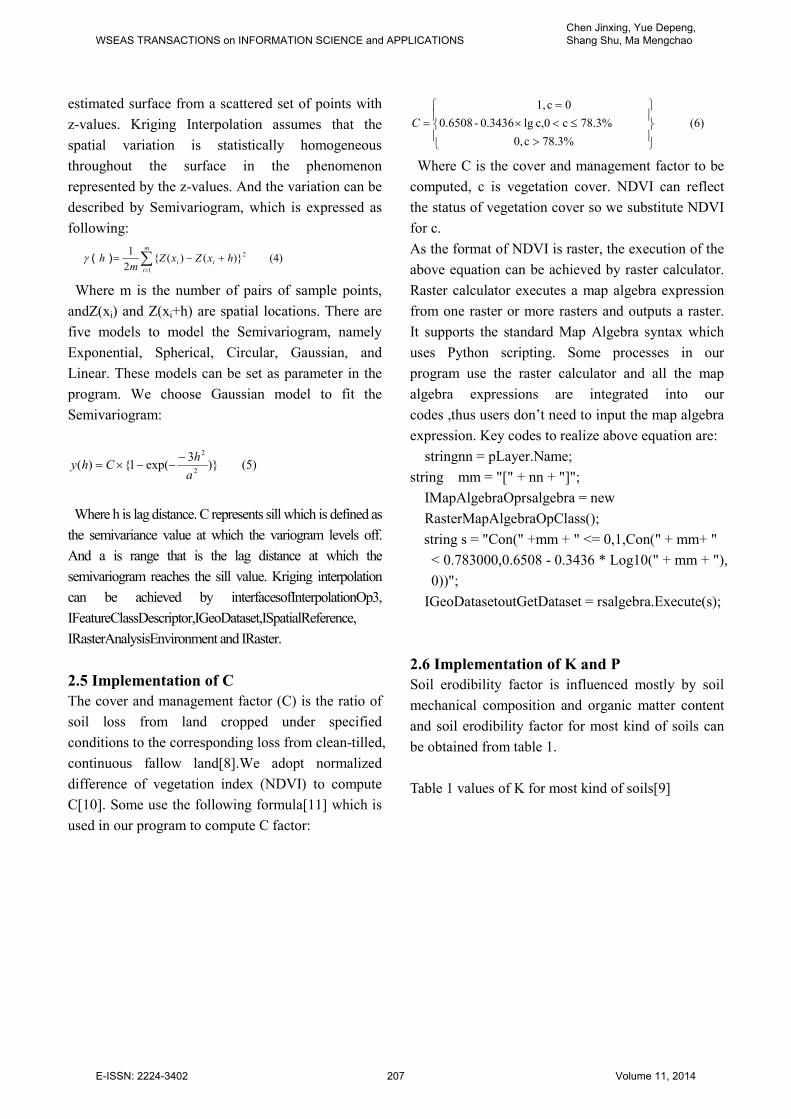
The main interface is shown in figure 3.Menu is on

the top, below which is toolbar. The submenus

execute the calculation of R、L、C、S factor and other

processings. Submenu soil lossscauculation calculate

the amount of soil loss. TocControl is on the

upper-left corner, which manage map layers.Values

of K and P are calculated by right clicking the layer

on the TocControl. The MapControl is on the middle,

which display maps. On the left bottom is Eagle Eye,

whose function is to locate the main map. The

bottom shows the current coordinate of x and y

whose unit is defined by the user.

Fig.3 The main interface

2.4 Implementation of R

R represents the potential capacity of rainfall to

cause erosion. We adopt the empirical equation of

Wischmeier’s [9]:

(2) 10735.1R12

1

8188.0lg5.1

2

∑ =

−×

×=i

p

pi

Where R is the erosivityvalue(MJ mm ha

-1h

-1·a

-1), pi

is the monthly precipitation amounts which can

produce soil erosion and p is the average

precipitation of the year. The rain records should

have monthly precipitation and average annual

precipitation will be calculated with R.

GE Zhong- qiang use another equation with a

different parameter to estimate soil lose in

Beijing[14] .

(3) 102157.1R12

1

8188.0lg5.1

2

∑ =

−×

×=i

p

pi

We provide these two equations in our program, it

depends on the regions and user can choose one to

estimate this factor. The rainfall record should be

shapefile format and R can be calculated by clicking

corresponding button.

Precipitation mainly comes from meteorological

stations which can’t cover the whole area. Therefore,

many unknown points exist. To obtain the soil loss

amount on the whole area, known precipitation

should be interpolated. We adopt Kriging

interpolation in our program, which generates an


E-ISSN: 2224-3402 206 Volume 11, 2014

estimated surface from a scattered set of points with

z-values. Kriging Interpolation assumes that the

spatial variation is statistically homogeneous

throughout the surface in the phenomenon

represented by the z-values. And the variation can be

described by Semivariogram, which is expressed as

following:

(4) )}()({2

1 2

1

hxZxZm

h i

m

i

i +−= ∑=

）（γ

Where m is the number of pairs of sample points,

andZ(xi) and Z(xi+h) are spatial locations. There are

five models to model the Semivariogram, namely

Exponential, Spherical, Circular, Gaussian, and

Linear. These models can be set as parameter in the

program. We choose Gaussian model to fit the

Semivariogram:

(5) )}3

exp(1{)(2

2

a

hChy

−−−×=

Where h is lag distance. C represents sill which is defined as

the semivariance value at which the variogram levels off.

And a is range that is the lag distance at which the

semivariogram reaches the sill value. Kriging interpolation

can be achieved by interfacesofInterpolationOp3,

IFeatureClassDescriptor,IGeoDataset,ISpatialReference,

IRasterAnalysisEnvironment and IRaster.

2.5 Implementation of C

The cover and management factor (C) is the ratio of

soil loss from land cropped under specified

conditions to the corresponding loss from clean-tilled,

continuous fallow land[8].We adopt normalized

difference of vegetation index (NDVI) to compute

C[10]. Some use the following formula[11] which is

used in our program to compute C factor:

(6)

78.3%c0,

78.3%cc,0 lg0.3436-0.6508

0c1,

>

≤<×

=

=C

Where C is the cover and management factor to be

computed, c is vegetation cover. NDVI can reflect

the status of vegetation cover so we substitute NDVI

for c.

As the format of NDVI is raster, the execution of the

above equation can be achieved by raster calculator.

Raster calculator executes a map algebra expression

from one raster or more rasters and outputs a raster.

It supports the standard Map Algebra syntax which

uses Python scripting. Some processes in our

program use the raster calculator and all the map

algebra expressions are integrated into our

codes ,thus users don’t need to input the map algebra

expression. Key codes to realize above equation are:

stringnn = pLayer.Name;

string mm = "[" + nn + "]";

IMapAlgebraOprsalgebra = new

RasterMapAlgebraOpClass();

string s = "Con(" +mm + " <= 0,1,Con(" + mm+ "

< 0.783000,0.6508 - 0.3436 * Log10(" + mm + "),

0))";

IGeoDatasetoutGetDataset = rsalgebra.Execute(s);

2.6 Implementation of K and P

Soil erodibility factor is influenced mostly by soil

mechanical composition and organic matter content

and soil erodibility factor for most kind of soils can

be obtained from table 1.

Table 1 values of K for most kind of soils[9]


E-ISSN: 2224-3402 207 Volume 11, 2014

Supporting practice factor(P) is calculated using

land use map. P is assigned a value according to the

land use type. The processing of P is similar to K.

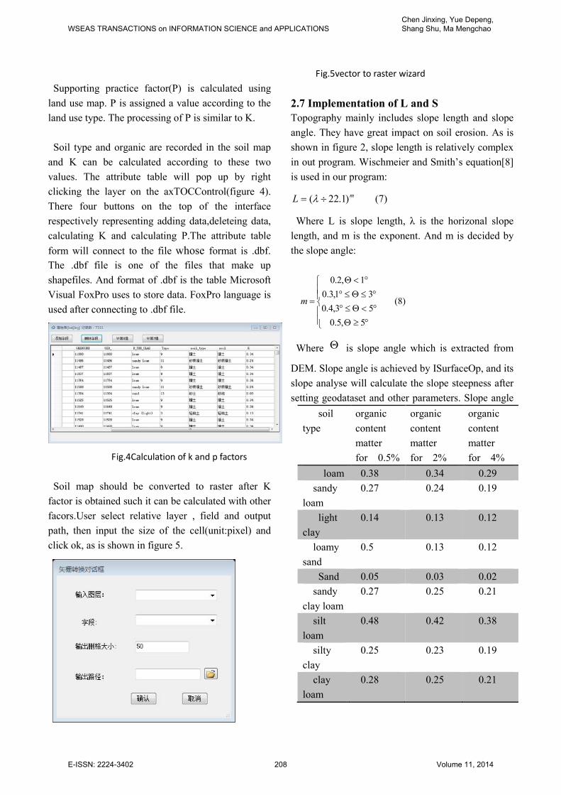
Soil type and organic are recorded in the soil map

and K can be calculated according to these two

values. The attribute table will pop up by right

clicking the layer on the axTOCControl(figure 4).

There four buttons on the top of the interface

respectively representing adding data,deleteing data,

calculating K and calculating P.The attribute table

form will connect to the file whose format is .dbf.

The .dbf file is one of the files that make up

shapefiles. And format of .dbf is the table Microsoft

Visual FoxPro uses to store data. FoxPro language is

used after connecting to .dbf file.

Fig.4Calculation of k and p factors

Soil map should be converted to raster after K

factor is obtained such it can be calculated with other

facors.User select relative layer , field and output

path, then input the size of the cell(unit:pixel) and

click ok, as is shown in figure 5.

Fig.5vector to raster wizard

2.7 Implementation of L and S

Topography mainly includes slope length and slope

angle. They have great impact on soil erosion. As is

shown in figure 2, slope length is relatively complex

in out program. Wischmeier and Smith’s equation[8]

is used in our program:

(7) )1.22(m

L ÷= λ

Where L is slope length, λ is the horizonal slope

length, and m is the exponent. And m is decided by

the slope angle:

(8)

5,5.0

53,4.0

31,3.0

1,2.0

°≥Θ

°<Θ≤°

°≤Θ≤°

°<Θ

=m

Where Θ is slope angle which is extracted from

DEM. Slope angle is achieved by ISurfaceOp, and its

slope analyse will calculate the slope steepness after

setting geodataset and other parameters. Slope angle

soil

type

organic

content

matter

for 0.5%

organic

content

matter

for 2%

organic

content

matter

for 4%

loam 0.38 0.34 0.29

sandy

loam

0.27 0.24 0.19

light

clay

0.14 0.13 0.12

loamy

sand

0.5 0.13 0.12

Sand 0.05 0.03 0.02

sandy

clay loam

0.27 0.25 0.21

silt

loam

0.48 0.42 0.38

silty

clay

0.25 0.23 0.19

clay

loam

0.28 0.25 0.21


E-ISSN: 2224-3402 208 Volume 11, 2014

factor(S) is obtained from the slope angle Θ ,and the

formula proposed by by McCool and Liu[12][13]:

(9)

10,96.0sin9.21

105,5.0sin8.16

5,036.0sin8.10

S

°≥Θ−Θ×

°<Θ≤°−Θ×

°<Θ+Θ×

=

This formula is executed by using raster calculator

in our program, which is similar to the computation

of C.

Wischmeier and Smith defined slope length as the

distance from the point of origin of overland flow to

the point where the slope decreases sufficiently for

deposition to occur[8]. Slope length can be divided

into many subsections and is calculated as follows:

(10) ,

,,

00∫=

jj

jj

yx

yxkyx dxλλ

Where jj yx ,λis the slope length at point (xj,yj), (x0,y0)

is the original point of overland flow, kλ is the

slope length at each grid alone the flow direction.

As shown in figure 2, the DEM is filled first.

Depressions exists in the DEM, which will block the

flow. After the DEM is filled ,the water will flow

fluently, which is shown in figure 6. A depression is

the lowest cell in the grid. The method of fill in the

interface of IHydrologyOp2 will execute this

function.

Fig.6 Fill the depression

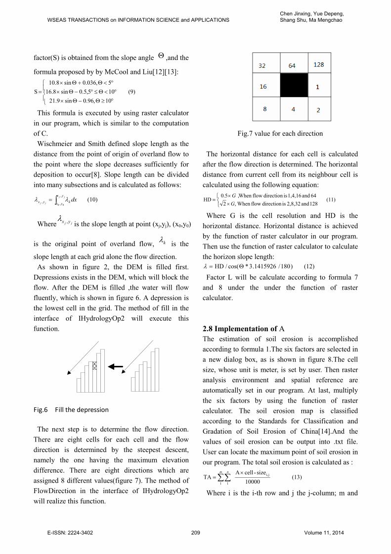
The next step is to determine the flow direction.

There are eight cells for each cell and the flow

direction is determined by the steepest descent,

namely the one having the maximum elevation

difference. There are eight directions which are

assigned 8 different values(figure 7). The method of

FlowDirection in the interface of IHydrologyOp2

will realize this function.

Fig.7 value for each direction

The horizontal distance for each cell is calculated

after the flow direction is determined. The horizontal

distance from current cell from its neighbour cell is

calculated using the following equation:

(11) 128 and 2,8,32 isdirection flow When ,2

64 and 1,4,16 isdirection flow When 5.0HD

×

×=

G

G，

Where G is the cell resolution and HD is the

horizontal distance. Horizontal distance is achieved

by the function of raster calculator in our program.

Then use the function of raster calculator to calculate

the horizon slope length:

(12) )180/1415926.3*cos(/HD Θ=λ

Factor L will be calculate according to formula 7

and 8 under the under the function of raster

calculator.

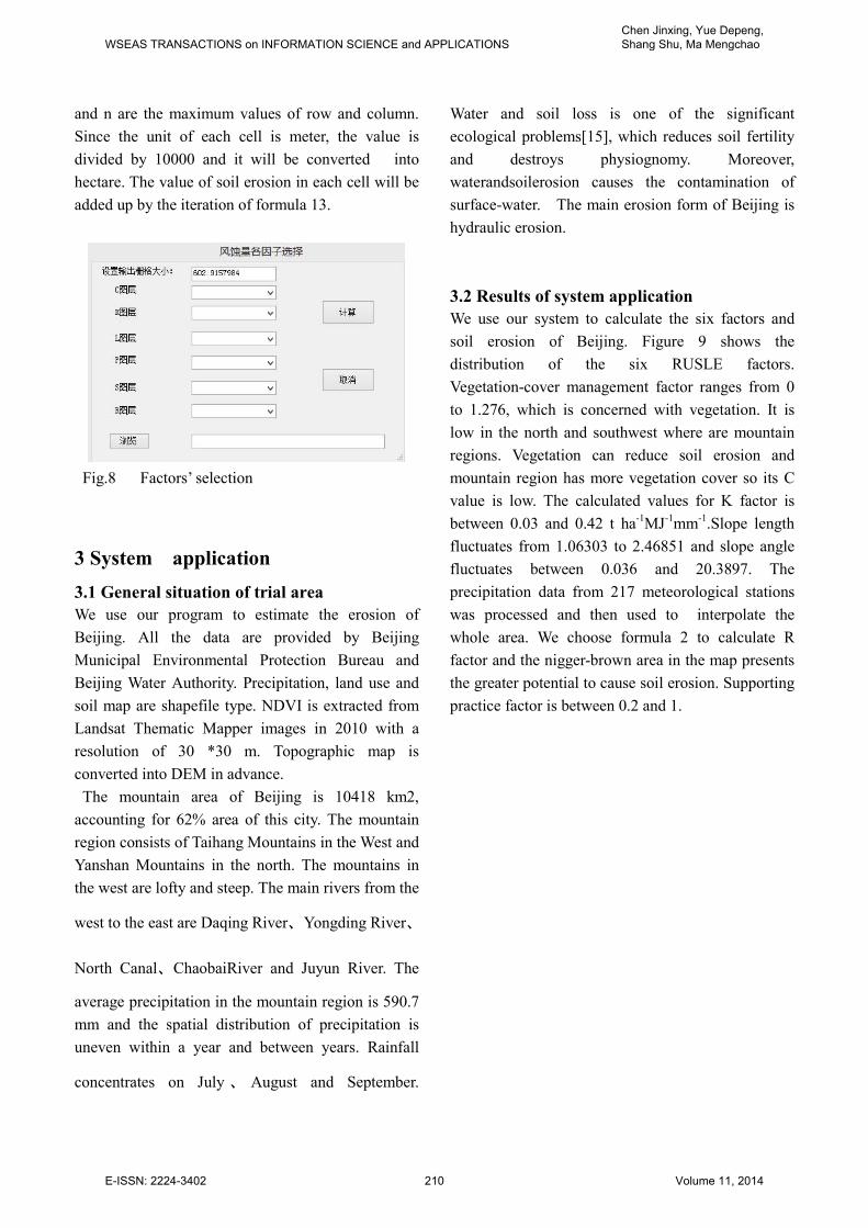
2.8 Implementation of A

The estimation of soil erosion is accomplished

according to formula 1.The six factors are selected in

a new dialog box, as is shown in figure 8.The cell

size, whose unit is meter, is set by user. Then raster

analysis environment and spatial reference are

automatically set in our program. At last, multiply

the six factors by using the function of raster

calculator. The soil erosion map is classified

according to the Standards for Classification and

Gradation of Soil Erosion of China[14].And the

values of soil erosion can be output into .txt file.

User can locate the maximum point of soil erosion in

our program. The total soil erosion is calculated as :

(13) 10000

size-cellATA

1

ji,

1

∑∑×

=m n

Where i is the i-th row and j the j-column; m and


E-ISSN: 2224-3402 209 Volume 11, 2014

and n are the maximum values of row and column.

Since the unit of each cell is meter, the value is

divided by 10000 and it will be converted into

hectare. The value of soil erosion in each cell will be

added up by the iteration of formula 13.

Fig.8 Factors’ selection

3 System application

3.1 General situation of trial area

We use our program to estimate the erosion of

Beijing. All the data are provided by Beijing

Municipal Environmental Protection Bureau and

Beijing Water Authority. Precipitation, land use and

soil map are shapefile type. NDVI is extracted from

Landsat Thematic Mapper images in 2010 with a

resolution of 30 *30 m. Topographic map is

converted into DEM in advance.

The mountain area of Beijing is 10418 km2,

accounting for 62% area of this city. The mountain

region consists of Taihang Mountains in the West and

Yanshan Mountains in the north. The mountains in

the west are lofty and steep. The main rivers from the

west to the east are Daqing River、Yongding River、

North Canal、ChaobaiRiver and Juyun River. The

average precipitation in the mountain region is 590.7

mm and the spatial distribution of precipitation is

uneven within a year and between years. Rainfall

concentrates on July 、 August and September.

Water and soil loss is one of the significant

ecological problems[15], which reduces soil fertility

and destroys physiognomy. Moreover,

waterandsoilerosion causes the contamination of

surface-water. The main erosion form of Beijing is

hydraulic erosion.

3.2 Results of system application

We use our system to calculate the six factors and

soil erosion of Beijing. Figure 9 shows the

distribution of the six RUSLE factors.

Vegetation-cover management factor ranges from 0

to 1.276, which is concerned with vegetation. It is

low in the north and southwest where are mountain

regions. Vegetation can reduce soil erosion and

mountain region has more vegetation cover so its C

value is low. The calculated values for K factor is

between 0.03 and 0.42 t ha-1

MJ-1

mm-1

.Slope length

fluctuates from 1.06303 to 2.46851 and slope angle

fluctuates between 0.036 and 20.3897. The

precipitation data from 217 meteorological stations

was processed and then used to interpolate the

whole area. We choose formula 2 to calculate R

factor and the nigger-brown area in the map presents

the greater potential to cause soil erosion. Supporting

practice factor is between 0.2 and 1.


E-ISSN: 2224-3402 210 Volume 11, 2014

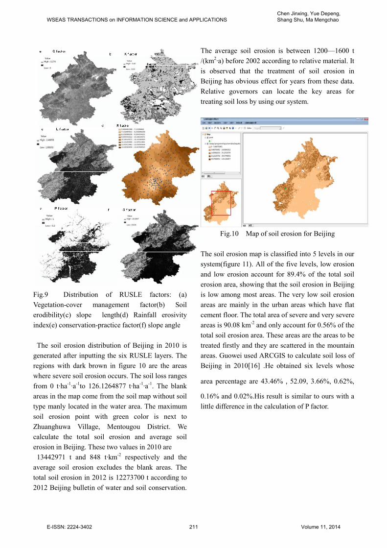
Fig.9 Distribution of RUSLE factors: (a)

Vegetation-cover management factor(b) Soil

erodibility(c) slope length(d) Rainfall erosivity

index(e) conservation-practice factor(f) slope angle

The soil erosion distribution of Beijing in 2010 is

generated after inputting the six RUSLE layers. The

regions with dark brown in figure 10 are the areas

where severe soil erosion occurs. The soil loss ranges

from 0 t·ha-1

·a-1

to 126.1264877 t·ha-1

·a-1

. The blank

areas in the map come from the soil map without soil

type manly located in the water area. The maximum

soil erosion point with green color is next to

Zhuanghuwa Village, Mentougou District. We

calculate the total soil erosion and average soil

erosion in Beijing. These two values in 2010 are

13442971 t and 848 t·km-2

respectively and the

average soil erosion excludes the blank areas. The

total soil erosion in 2012 is 12273700 t according to

2012 Beijing bulletin of water and soil conservation.

The average soil erosion is between 1200—1600 t

/(km2·a) before 2002 according to relative material. It

is observed that the treatment of soil erosion in

Beijing has obvious effect for years from these data.

Relative governors can locate the key areas for

treating soil loss by using our system.

Fig.10 Map of soil erosion for Beijing

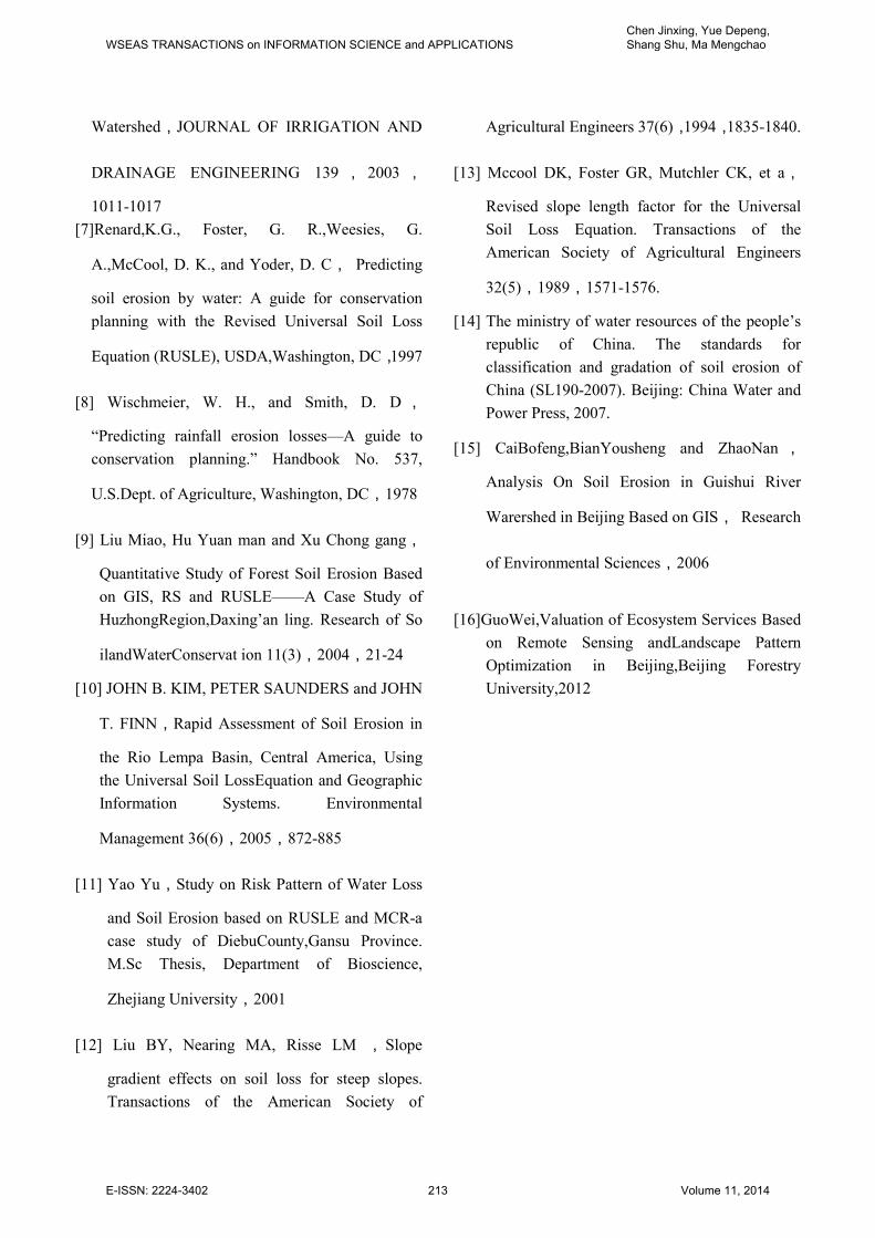
The soil erosion map is classified into 5 levels in our

system(figure 11). All of the five levels, low erosion

and low erosion account for 89.4% of the total soil

erosion area, showing that the soil erosion in Beijing

is low among most areas. The very low soil erosion

areas are mainly in the urban areas which have flat

cement floor. The total area of severe and very severe

areas is 90.08 km-2

and only account for 0.56% of the

total soil erosion area. These areas are the areas to be

treated firstly and they are scattered in the mountain

areas. Guowei used ARCGIS to calculate soil loss of

Beijing in 2010[16] .He obtained six levels whose

area percentage are 43.46%，52.09, 3.66%, 0.62%,

0.16% and 0.02%.His result is similar to ours with a

little difference in the calculation of P factor.


E-ISSN: 2224-3402 211 Volume 11, 2014

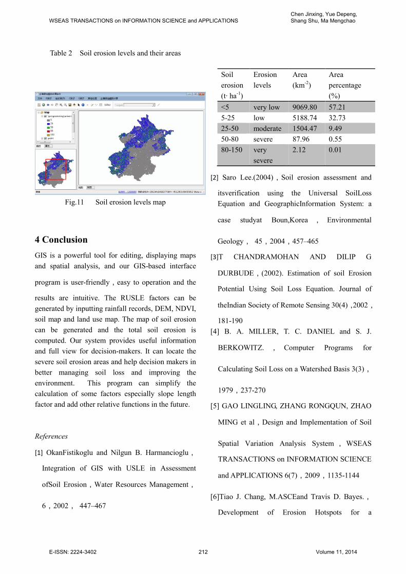
Table 2 Soil erosion levels and their areas

Fig.11 Soil erosion levels map

4 Conclusion

GIS is a powerful tool for editing, displaying maps

and spatial analysis, and our GIS-based interface

program is user-friendly，easy to operation and the

results are intuitive. The RUSLE factors can be

generated by inputting rainfall records, DEM, NDVI,

soil map and land use map. The map of soil erosion

can be generated and the total soil erosion is

computed. Our system provides useful information

and full view for decision-makers. It can locate the

severe soil erosion areas and help decision makers in

better managing soil loss and improving the

environment. This program can simplify the

calculation of some factors especially slope length

factor and add other relative functions in the future.

References

[1] OkanFistikoglu and Nilgun B. Harmancioglu，

Integration of GIS with USLE in Assessment

ofSoil Erosion，Water Resources Management，

6，2002， 447–467

[2] Saro Lee.(2004)，Soil erosion assessment and

itsverification using the Universal SoilLoss

Equation and GeographicInformation System: a

case studyat Boun,Korea ， Environmental

Geology， 45，2004，457–465

[3]T CHANDRAMOHAN AND DILIP G

DURBUDE，(2002). Estimation of soil Erosion

Potential Using Soil Loss Equation. Journal of

theIndian Society of Remote Sensing 30(4)，2002，

181-190

[4] B. A. MILLER, T. C. DANIEL and S. J.

BERKOWITZ. ， Computer Programs for

Calculating Soil Loss on a Watershed Basis 3(3)，

1979，237-270

[5] GAO LINGLING, ZHANG RONGQUN, ZHAO

MING et al，Design and Implementation of Soil

Spatial Variation Analysis System ， WSEAS

TRANSACTIONS on INFORMATION SCIENCE

and APPLICATIONS 6(7)，2009，1135-1144

[6]Tiao J. Chang, M.ASCEand Travis D. Bayes.，

Development of Erosion Hotspots for a

Soil

erosion

(t· ha-1

)

Erosion

levels

Area

(km-2

)

Area

percentage

(%)

<5 very low 9069.80 57.21

5-25 low 5188.74 32.73

25-50 moderate 1504.47 9.49

50-80 severe 87.96 0.55

80-150 very

severe

2.12 0.01


E-ISSN: 2224-3402 212 Volume 11, 2014

Watershed，JOURNAL OF IRRIGATION AND

DRAINAGE ENGINEERING 139 ， 2003 ，

1011-1017

[7]Renard,K.G., Foster, G. R.,Weesies, G.

A.,McCool, D. K., and Yoder, D. C， Predicting

soil erosion by water: A guide for conservation

planning with the Revised Universal Soil Loss

Equation (RUSLE), USDA,Washington, DC，1997

[8] Wischmeier, W. H., and Smith, D. D ，

“Predicting rainfall erosion losses—A guide to

conservation planning.” Handbook No. 537,

U.S.Dept. of Agriculture, Washington, DC，1978

[9] Liu Miao, Hu Yuan man and Xu Chong gang，

Quantitative Study of Forest Soil Erosion Based

on GIS, RS and RUSLE——A Case Study of

HuzhongRegion,Daxing’an ling. Research of So

ilandWaterConservat ion 11(3)，2004，21-24

[10] JOHN B. KIM, PETER SAUNDERS and JOHN

T. FINN，Rapid Assessment of Soil Erosion in

the Rio Lempa Basin, Central America, Using

the Universal Soil LossEquation and Geographic

Information Systems. Environmental

Management 36(6)，2005，872-885

[11] Yao Yu，Study on Risk Pattern of Water Loss

and Soil Erosion based on RUSLE and MCR-a

case study of DiebuCounty,Gansu Province.

M.Sc Thesis, Department of Bioscience,

Zhejiang University，2001

[12] Liu BY, Nearing MA, Risse LM ， Slope

gradient effects on soil loss for steep slopes.

Transactions of the American Society of

Agricultural Engineers 37(6)，1994，1835-1840.

[13] Mccool DK, Foster GR, Mutchler CK, et a，

Revised slope length factor for the Universal

Soil Loss Equation. Transactions of the

American Society of Agricultural Engineers

32(5)，1989，1571-1576.

[14] The ministry of water resources of the people’s

republic of China. The standards for

classification and gradation of soil erosion of

China (SL190-2007). Beijing: China Water and

Power Press, 2007.

[15] CaiBofeng,BianYousheng and ZhaoNan ，

Analysis On Soil Erosion in Guishui River

Warershed in Beijing Based on GIS， Research

of Environmental Sciences，2006

[16]GuoWei,Valuation of Ecosystem Services Based

on Remote Sensing andLandscape Pattern

Optimization in Beijing,Beijing Forestry

University,2012


E-ISSN: 2224-3402 213 Volume 11, 2014

Documents

Design and Implementation of Soil Loss System Based on RUSLE