sustainability

Article

Comparison of RUSLE and MMF Soil Loss Models andEvaluation of Catchment Scale Best Management Practices for aMountainous Watershed in India

Susanta Das 1 , Proloy Deb 2,* , Pradip Kumar Bora 3 and Prafull Katre 4

�����������������

Citation: Das, S.; Deb, P.; Bora, P.K.;

Katre, P. Comparison of RUSLE and

MMF Soil Loss Models and

Evaluation of Catchment Scale Best

Management Practices for a

Mountainous Watershed in India.

Sustainability 2021, 13, 232. https://

doi.org/10.3390/su13010232

Received: 19 September 2020

Accepted: 16 December 2020

Published: 29 December 2020

Publisher’s Note: MDPI stays neu-

tral with regard to jurisdictional claims

in published maps and institutional

affiliations.

Copyright: © 2020 by the authors. Li-

censee MDPI, Basel, Switzerland. This

article is an open access article distributed

under the terms and conditions of the

Creative Commons Attribution (CC BY)

license (https://creativecommons.org/

licenses/by/4.0/).

1 Department of Soil and Water Engineering, Punjab Agricultural University, Ludhiana, Punjab 141004, India;susanta-swe@pau.edu

2 Centre for Complex Hydrosystems Research, Department of Civil, Construction andEnvironmental Engineering, The University of Alabama, Tuscaloosa, AL 35487, USA

3 College of Post Graduate Studies, Central Agricultural University, Umiam, Meghalaya 793103, India;pradip66@gmail.com

4 Department of Soil and Water Engineering, Swami Vivekanand College of AgriculturalEngineering & Technology, Indira Gandhi Krishi Vishwavidyalaya, Raipur, Chhattisgarh 492012, India;prafullkatre@rediffmail.com

* Correspondence: pdeb1@ua.edu

Abstract: Soil erosion from arable lands removes the top fertile soil layer (comprised of humus/organicmatter) and therefore requires fertilizer application which affects the overall sustainability. Hence,determination of soil erosion from arable lands is crucial to planning conservation measures. A mod-eling approach is a suitable alternative to estimate soil loss in ungauged catchments. Soil erosionprimarily depends on soil texture, structure, infiltration, topography, land uses, and other erosiveforces like water and wind. By analyzing these parameters, coupled with geospatial tools, modelscan estimate storm wise and annual average soil losses. In this study, a hilly watershed calledNongpoh was considered with the objective of prioritizing critical erosion hazard areas withinthe micro-catchment based on average annual soil loss and land use and land cover and makingappropriate management plans for the prioritized areas. Two soil erosion models namely RevisedUniversal Soil Loss Equation (RUSLE) and Modified Morgan–Morgan–Finney (MMF) models wereused to estimate soil loss with the input parameters extracted from satellite information and auto-matic weather stations. The RUSLE and MMF models showed similar results in estimating soil loss,except the MMF model estimated 7.74% less soil loss than the RUSLE model from the watershed.The results also indicated that the study area is under severe erosion class, whereas agricultural land,open forest area, and scrubland were prioritized most erosion prone areas within the watershed.Based on prioritization, best management plans were developed at catchment scale for reducing soilloss. These findings and the methodology employed can be widely used in mountainous to hillywatersheds around the world for identifying best management practices (BMP).

Keywords: soil erosion; LULC; RUSLE; MMF; prioritization and management plan

1. Introduction

Soil loss resulting from erosion is a universal issue which affects agricultural produc-tion and natural resources [1,2]. Degradation of soil physical properties by soil erosioncan affect the crop growth and yield by reducing the root depth, available water, and nu-trient reserves, and also by affecting soil organic carbon, phosphorus, potassium, nitrogencontents, and pH [3]. It also carries soil-laden water downstream, which can produceheavy deposits of sediment that prevent the smooth flow of rivers and streams and caneventually lead to floods [2]. Soil erosion occurs when soil particles are carried off bywater or wind and deposited elsewhere. Water erosion begins once rain or irrigation waterdetaches soil particles. Once there is an excessive amount of water on the soil surface,

Sustainability 2021, 13, 232. https://doi.org/10.3390/su13010232 https://www.mdpi.com/journal/sustainability

Sustainability 2021, 13, 232 2 of 22

it fills surface depressions and begins to flow with enough speed; this surface runoffcarries away the loose soil.

The erosion process is influenced by numerous factors, primarily anthropogenic,such as urbanization and mining, and by natural causes, such as flash floods, and rain-storms [2,4,5]. The estimation of these factors is crucial to grasp the individual impact ofthe factors and establish the crucial sub-watershed in order for proper management andconservation measures to be planned to mitigate erosion [6]. As soil erosion is a continuousprocess and is non-linear in nature, the assessment of its environmental impact is ambigu-ous. In order to address this non-linearity, several complex biophysical developments(in terms of modeling) have been done. However, it is still uncertain how and where thesoil erosion occurs [7]. Additionally, soil erosion is proportional to population growth,overuse of natural resources, degraded land, and poor water management plans [8–10].A prerequisite of soil conservation is the reversal of land desertion and the enhancementof agricultural production, the provision of food sanctuary, and sustainability, therebyrequiring identification of critical erosion prone areas. In addition to soil degradation,other difficulties caused by soil erosion include removal of soil nutrients, decline of cropyields, reduction of soil fertility, and contamination of surface and groundwater suppliesby fertilizer nutrients, sediment, and insecticide residues [4].

Numerous methods are available for quantifying soil erosion. These methods aregenerally physical or experimental/laboratory scale models [11,12]. The Water Erosion Pre-diction Project (WEPP) [13], the European Soil Erosion Model (EUROSEM) [6], and the Lim-burg Soil Erosion Model (LISEM) [14] have mainly used physical-based models. Since thesemethods are based on actual procedures, they require a large number of input parameterswith comprehensive computation. Therefore, simulation of these for a particular area re-quires data on the observed sediment loss which are not available for ungauged watershedsand in many developing and less developed countries [15]. On the other hand, empiricalmodels such as Universal Soil Loss Equation (USLE) [16], Modified Morgan–Morgan–Finney (MMF) [17], and Revised Universal Soil Loss Equation (RUSLE) [18] provide analternative to relate the soil loss to several physical components which are relatively easyto calculate/estimate.

Unlike USLE which inherits a number of limitations including point scale soil lossestimation and mainly targeted for agricultural lands, RUSLE has the advantage of inte-grating remote sensing (RS) and geographic information systems (GIS) to assess the risk ofpotential soil erosion at a spatial scale [19,20]. This empirical approach is widely acceptedby the soil erosion community due to its simplicity and limited data requirement [4,21–25].GIS information layers as well as, rainfall erosivity (R), soil erodibility (K), slope lengthand gradient (LS), crop management (C), and conservation practice (P) factors can be inte-grated within the ArcGIS platform to evaluate the collaborative influence on the averageannual soil loss.

Similarly, the MMF model is another model like RUSLE, which is aimed at makingmuch use of the physically based concept provided by Meyer and Wischmeier (1969) [26]as compared to the USLE [16,27]. The modified MMF model separates the eroding methodinto two sections: the water phase and the sediment phase. The water phase determinesthe energy of rain offered to detach soil particles from the soil mass and carried with thesurface runoff. The erosion phase regulates the rate of soil particle detachment by rain andrunoff and is determined in conjunction with the transport capability of runoff [17,28–30].This model is highly sensitive to the annual rain and soil parameters, once erosion istransport-limited [17]. Mapping of soil erodibility at a spatial scale is possible by integratingRS and GIS techniques with RUSLE and MMF models, which can be further used inidentifying the potential risk of soil erosion at a larger geographical extent. The formulationof correct soil management for property development needs a precise inventory and ratingof vulnerable areas. These data are incredibly helpful within the higher cognitive processcontext to avoid land degradation in erosion risk areas, or, as an alternative, to suggestconservation measures to reduce the soil loss if developments continue.

Sustainability 2021, 13, 232 3 of 22

Given the difference in the model structures and their inherent limitations, it is criticalto identify which soil loss model is more suitable for mountainous catchments in India.Therefore, in this study, a peri-urban watershed in high rainfall areas of Meghalaya, which isclose to Nongpoh, district headquarters of Ri-Bhoi district, was taken for estimating erosion.The farmers are found to extend their cultivations in many other places within the studywatershed. Even some crops like rice, pineapple, and tomato cultivation have been startedin the foot hills areas of the watershed. As the study area is a peri-urban watershed witha high degree of slope and the site usually receives a high amount of rainfall, there isclearly pressure on the natural resources of watershed. Given the high slope aided withhigh rainfall combined with anthropogenic activities, the study area (and also the entireMeghalaya state) is losing the fertile topsoil layer contributing to the deterioration of soilhealth from an agricultural perspective [31,32]. Hence it has become paramount to quantifythe soil loss and make the best management plan for maintaining the sustainability ofthe land and improving the agricultural production in the study area. Both RUSLE andMMF models were used for estimating soil erosion and identifying the erosion prone areaswith the following objectives: (1) to prioritize the critical erosion hazard areas within themicro-catchment based on average annual soil loss, land use, and land cover, and (2) tomake the appropriate management plans for the prioritized area. The findings of this studywill aid in developing best management practice plans for the watershed for maintainingoverall agricultural sustainability by improving soil health and reducing the application offertilizers/manures for enhanced crop yields.

2. Materials and Methods2.1. Description of the Study Area

The study area is a micro-catchment situated at Nongpoh of Ri-Bhoi district, Megha-laya. The study area lies between 25◦54′0” to 25◦55′05” N latitude and 91◦52′54.7” to91◦54′17.7” E longitude and it covers an area of 268 ha (2.68 km2). The study area fallsunder a humid subtropical climate. The area receives a mean annual rainfall of about2700 mm, 77% of which is received from July to September [33]. The study area has anaverage elevation of 469–760 m above the mean sea level (MSL). The relief is moderateto steeply sloping and the drainage condition varies from well drained in upland areasto poorly drained in low lying areas. The location of the study area is shown in Figure 1.Additionally, Table 1 illustrates the mean monthly and average annual precipitation at fourdifferent rain gauges near the micro-catchment. The average precipitation values werederived for a period of 9 years, i.e., 2010–2019. Figure 2 showcases the severity of soilerosion in the study catchment.

The Nongpoh micro-catchment is classified into seven slope classes i.e., flat (0–3%),undulating (3–8%), moderately slope (8–15%), hilly 105 ◦C for 24 h and then samples wereweighted, (15–30%), moderately steep slope (30–45%), steep slope (45–60%), and very steepslope (>60%) as per the recommendations of Lee and Silalahi et al. [34,35]. The slope mapof Nongpoh micro-catchment is displayed in Figure 3a. Additionally, Figure 3b displaysthe hypsometric map of the study area. It can be seen that the contours representing higherelevation (ranging from 540 to 760) are more dominant in the edges of the catchment.

Sustainability 2021, 13, 232 4 of 22Sustainability 2020, 12, x FOR PEER REVIEW 4 of 22

Figure 1. (a) India, (b) Meghalaya, (c) Ri-Bhoi District, and (d) Nongpoh micro-catchment.

Table 1. Mean monthly and average annual rainfall (mm) of stations in the study area.

Month Byrnihat (mm) Nongpoh (mm) Umsining (mm) NESAC * (mm)

January 6.91 16.91 18.75 16.33

February 12.16 20.16 20.25 25.21

March 45.78 48.79 42.25 59.25

April 134.62 126.55 51.75 98.60

May 244.35 204.00 239.25 428.60

June 547.80 580.80 527.75 430.20

July 581.49 615.35 575.75 572.20

August 528.62 548.62 455.25 510.25

September 418.25 413.25 396.25 492.25

October 136.73 146.73 149.50 170.50

November 12.43 14.42 13.25 37.33

December 10.72 19.21 18.50 14.67

Yearly 2679.86 2754.80 2508.50 2855.39

* NESAC stands for North-Eastern Space Applications Centre.

(a) (b)

Figure 1. (a) India, (b) Meghalaya, (c) Ri-Bhoi District, and (d) Nongpoh micro-catchment.

Table 1. Mean monthly and average annual rainfall (mm) of stations in the study area.

Month Byrnihat (mm) Nongpoh (mm) Umsining (mm) NESAC * (mm)

January 6.91 16.91 18.75 16.33February 12.16 20.16 20.25 25.21

March 45.78 48.79 42.25 59.25April 134.62 126.55 51.75 98.60May 244.35 204.00 239.25 428.60June 547.80 580.80 527.75 430.20July 581.49 615.35 575.75 572.20

August 528.62 548.62 455.25 510.25September 418.25 413.25 396.25 492.25

October 136.73 146.73 149.50 170.50November 12.43 14.42 13.25 37.33December 10.72 19.21 18.50 14.67

Yearly 2679.86 2754.80 2508.50 2855.39* NESAC stands for North-Eastern Space Applications Centre.

Sustainability 2020, 12, x FOR PEER REVIEW 4 of 22

Figure 1. (a) India, (b) Meghalaya, (c) Ri-Bhoi District, and (d) Nongpoh micro-catchment.

Table 1. Mean monthly and average annual rainfall (mm) of stations in the study area.

Month Byrnihat (mm) Nongpoh (mm) Umsining (mm) NESAC * (mm)

January 6.91 16.91 18.75 16.33

February 12.16 20.16 20.25 25.21

March 45.78 48.79 42.25 59.25

April 134.62 126.55 51.75 98.60

May 244.35 204.00 239.25 428.60

June 547.80 580.80 527.75 430.20

July 581.49 615.35 575.75 572.20

August 528.62 548.62 455.25 510.25

September 418.25 413.25 396.25 492.25

October 136.73 146.73 149.50 170.50

November 12.43 14.42 13.25 37.33

December 10.72 19.21 18.50 14.67

Yearly 2679.86 2754.80 2508.50 2855.39

* NESAC stands for North-Eastern Space Applications Centre.

(a) (b)

Figure 2. Cont.

Sustainability 2021, 13, 232 5 of 22

Sustainability 2020, 12, x FOR PEER REVIEW 5 of 22

Figure 2. Severity of soil erosion in (a) open forest; (b) dense forest; (c) settlement; and (d) agriculture land use classes at

the study catchment.

Figure 3. (a) Slope map and (b) hypsometric map of the study area.

The observed soil loss data were obtained for the years 2010–2019 from an ongoing

research project of College of Post Graduate Studies (CPGS), Central Agricultural

University, Meghalaya, India. After each rainstorm, depth of runoff data were collected

at the catchment outlet and, using a measuring cylinder of one liter of water samples,

were taken for determination of soil loss. Post-collection of the samples, they were

filtered through filter paper of 42 no. grade and the soil was separated from the water.

Thereby, the soil was kept in an oven at 105 °C for 24 h and then samples were weighed.

The methodological flowchart is given in Figure 4. First, the digital elevation model

(DEM) having a spatial resolution of 2.5 m derived from CARTOSAT-1 (downloaded

from Bhuvan, https://bhuvan-app3.nrsc.gov.in/data/download/) was used in identifying

the slope and catchment delineation. Additionally, the land use land covers (LULC) for

the catchment was derived from the satellite image of Linear Imaging Self-Scanning

(c) (d)

Figure 2. Severity of soil erosion in (a) open forest; (b) dense forest; (c) settlement; and (d) agriculture land use classes at thestudy catchment.

Sustainability 2020, 12, x FOR PEER REVIEW 5 of 22

Figure 2. Severity of soil erosion in (a) open forest; (b) dense forest; (c) settlement; and (d) agriculture land use classes at

the study catchment.

Figure 3. (a) Slope map and (b) hypsometric map of the study area.

The observed soil loss data were obtained for the years 2010–2019 from an ongoing

research project of College of Post Graduate Studies (CPGS), Central Agricultural

University, Meghalaya, India. After each rainstorm, depth of runoff data were collected

at the catchment outlet and, using a measuring cylinder of one liter of water samples,

were taken for determination of soil loss. Post-collection of the samples, they were

filtered through filter paper of 42 no. grade and the soil was separated from the water.

Thereby, the soil was kept in an oven at 105 °C for 24 h and then samples were weighed.

The methodological flowchart is given in Figure 4. First, the digital elevation model

(DEM) having a spatial resolution of 2.5 m derived from CARTOSAT-1 (downloaded

from Bhuvan, https://bhuvan-app3.nrsc.gov.in/data/download/) was used in identifying

the slope and catchment delineation. Additionally, the land use land covers (LULC) for

the catchment was derived from the satellite image of Linear Imaging Self-Scanning

(c) (d)

Figure 3. (a) Slope map and (b) hypsometric map of the study area.

The observed soil loss data were obtained for the years 2010–2019 from an ongoingresearch project of College of Post Graduate Studies (CPGS), Central Agricultural Univer-sity, Meghalaya, India. After each rainstorm, depth of runoff data were collected at thecatchment outlet and, using a measuring cylinder of one liter of water samples, were takenfor determination of soil loss. Post-collection of the samples, they were filtered throughfilter paper of 42 no. grade and the soil was separated from the water. Thereby, the soilwas kept in an oven at 105 ◦C for 24 h and then samples were weighed.

The methodological flowchart is given in Figure 4. First, the digital elevation model(DEM) having a spatial resolution of 2.5 m derived from CARTOSAT-1 (downloaded fromBhuvan, https://bhuvan-app3.nrsc.gov.in/data/download/) was used in identifying theslope and catchment delineation. Additionally, the land use land covers (LULC) for thecatchment was derived from the satellite image of Linear Imaging Self-Scanning SystemIV (LISS-IV) for the year 2015. With the identified characteristics of the catchment and the

Sustainability 2021, 13, 232 6 of 22

RUSLE and MMF model parameters derived within the catchment, the rate of soil loss forthe years 2010 to 2019 year was calculated, which was further used in the model calibrationand validation. Moreover, based on the estimated rate of soil erosion, the prioritizedmicro-catchments were chosen, and using ArcGIS 10.2, several best management practicesfor reducing soil loss at the micro-catchment were conducted.

Sustainability 2020, 12, x FOR PEER REVIEW 6 of 22

System IV (LISS-IV) for the year 2015. With the identified characteristics of the catchment

and the RUSLE and MMF model parameters derived within the catchment, the rate of

soil loss for the years 2010 to 2019 year was calculated, which was further used in the

model calibration and validation. Moreover, based on the estimated rate of soil erosion,

the prioritized micro-catchments were chosen, and using ArcGIS 10.2, several best

management practices for reducing soil loss at the micro-catchment were conducted.

Figure 4. Methodological flowchart of the study.

2.2. Land Use Land Cover

Based on tonal and color variation in the satellite imagery (LISS-IV, 8-12-2015) and

ground-truthing (supervised classification), the major LULC classes were identified. The

spatial distribution of LULC categories, such as contour bunding, agriculture, dense

forest, open forest, settlement, scrubland, terrace farming, upland paddy field,

waterbody, etc., is prepared by 1:5000 scales. The land use land cover map of Nongpoh is

shown in Figure 5. The data on the statistics of the LULC categories identified in

Nongpoh micro-catchment are presented in Table 2.

Table 2. Land use land cover (LULC) classes of the study area.

LULC Area (ha) Area (%)

Contour bunding 4.20 1.57

Agriculture 44.29 16.52

Dense forest 78.80 29.39

Open forest 55.15 20.57

Settlement 49.37 18.41

Scrubland 26.48 9.88

Terrace farming 0.19 0.07

Figure 4. Methodological flowchart of the study.

2.2. Land Use Land Cover

Based on tonal and color variation in the satellite imagery (LISS-IV, 8-12-2015) andground-truthing (supervised classification), the major LULC classes were identified. The spa-tial distribution of LULC categories, such as contour bunding, agriculture, dense forest,open forest, settlement, scrubland, terrace farming, upland paddy field, waterbody, etc.,is prepared by 1:5000 scales. The land use land cover map of Nongpoh is shown in Figure 5.The data on the statistics of the LULC categories identified in Nongpoh micro-catchmentare presented in Table 2.

Table 2. Land use land cover (LULC) classes of the study area.

LULC Area (ha) Area (%)

Contour bunding 4.20 1.57Agriculture 44.29 16.52Dense forest 78.80 29.39Open forest 55.15 20.57Settlement 49.37 18.41Scrubland 26.48 9.88

Terrace farming 0.19 0.07Upland paddy field 8.86 3.30

Water body 0.81 0.30Total 268.15 100.00

Sustainability 2021, 13, 232 7 of 22

Sustainability 2020, 12, x FOR PEER REVIEW 7 of 22

Upland paddy field 8.86 3.30

Water body 0.81 0.30

Total 268.15 100.00

Figure 5. LULC of the study area.

2.3. Estimation of Soil Loss

2.3.1. Revised Universal Soil Loss Equation (RUSLE)

RUSLE is the method that is the most widely used approach in estimating long-term

rates of inter-rill and rill erosion from field or farm size units subject to different

management practices. The underlying assumption in RUSLE is that the detachment and

deposition are controlled by sediment content in the runoff. The equation has following

form, Equation (1).

A = R × K × LS × C × P (1)

where A = average annual soil loss (t h−1 yr−1), R = rainfall and runoff erosivity (MJ mm

ha−1 h−1 yr−1), K = soil erodibility factor, LS = topographic factor, C = crop management

factor, and P = supporting conservation practice factor.

Rainfall and Runoff Erosivity (R)

Rainfall plays a significant role in the process of soil erosion and sedimentation, and

this ultimately contributes to water erosion including splash, sheet, rill, and gully

erosion, triggered by water flow. The erosive force of rainfall which causes soil erosion is

known as rainfall erosivity factor (R). The data of monthly rainfall (shown in Table 2) and

annual rainfall are used for the calculation of R factor using Equation (2) [17,36]. The

spatial variability of R is calculated in ArcGIS 10.2 domain using a spatial interpolation

tool for the study area.

R = ∑ 1.735 × 10(1.5 log10(

pi2

P− 0.08188))

121

(2)

Figure 5. LULC of the study area.

2.3. Estimation of Soil Loss2.3.1. Revised Universal Soil Loss Equation (RUSLE)

RUSLE is the method that is the most widely used approach in estimating long-term rates of inter-rill and rill erosion from field or farm size units subject to differentmanagement practices. The underlying assumption in RUSLE is that the detachment anddeposition are controlled by sediment content in the runoff. The equation has followingform, Equation (1).

A = R × K × LS × C × P (1)

where A = average annual soil loss (t h−1 yr−1), R = rainfall and runoff erosivity(MJ mm ha−1 h−1 yr−1), K = soil erodibility factor, LS = topographic factor, C = cropmanagement factor, and P = supporting conservation practice factor.

Rainfall and Runoff Erosivity (R)

Rainfall plays a significant role in the process of soil erosion and sedimentation,and this ultimately contributes to water erosion including splash, sheet, rill, and gullyerosion, triggered by water flow. The erosive force of rainfall which causes soil erosion isknown as rainfall erosivity factor (R). The data of monthly rainfall (shown in Table 2) andannual rainfall are used for the calculation of R factor using Equation (2) [17,36]. The spatialvariability of R is calculated in ArcGIS 10.2 domain using a spatial interpolation tool forthe study area.

R =12

∑1

1.735 × 10(1.5 log10 (pi

2

P − 0.08188)) (2)

where pi = monthly rainfall (mm) and P = annual rainfall (mm), and R = Rainfall and runofferosivity (MJ mm ha−1 h−1 yr−1).

Sustainability 2021, 13, 232 8 of 22

Soil Erodibility Factor (K)

Soil erodibility factor (K) is influenced by the geological characteristics, such as parentmaterial, texture, structure, organic matter content, and porosity of the soil. As silt isthe primary particle responsible for soil erosion, erodibility tends to decrease with thedecrease of silt particle in the soil, irrespective of % content of sand and clay [33–37].For the calculation of K factor of the study area, the soil physical properties analysesequation [38] was adopted. In this method, physical properties of soil such as soil texture,soil structure, soil permeability, and soil organic matter are used to calculate the K factor [33].Other researchers also used this equation [33,36,37,39,40]. The soil sample was collectedfrom the 50 different places of the watershed to calculate the physical properties of thesoil. The laboratory analysis was done for all the parameters following the procedure ofDeb et al. [40], and then this point value was taken in the ArcGIS domain. The K factorwas calculated by using raster calculator, spatial interpolation (kriging) technique, and wascalculated as in Equation (3).

K = 27.66×M1.14 × 10−8 × (12− a) + 0.0043× (b− 2) + 0.0033× (c− 3) (3)

where K = soil erodibility factor, M = (silt (%) + very fine sand (%) × (100-clay%)),a = organic matter (%), b = soil structure, and c = soil permeability (1—rapid, 2—moderateto rapid, 3—moderate, 4—moderate to slow, 5—slow, and 6—very slow].

Topographic Factor (LS)

The LS factor represents the ratio of soil loss on a given slope length and steepnessto soil loss from a slope that has a length of 22.1 m and steepness of 9%, where all otherconditions are the same [35]. The LS factor is not an absolute value, instead is referenced tounity at 22.1 m slope length and 9% steepness, and hence provides significant informationon the susceptibility of the terrain to soil erosion. The LS factor was computed [16,35] usingthe Equation (4).

LS =

(λ

22.13

)m×

(0.065 + 0.045 S + 0.0065 S2

)(4)

where λ = slope length (m), S = angle of slope (%), m is the constant dependent on thevalue of the slope gradient; 0.5 if the slope angle is greater than 5%, 0.4 on slopes of 3% to5%, 0.3 on slopes of 1 to 3%, and 0.2 on slopes less than 1%.

Crop Management Factor (C)

The crop management factor (C) is used to determine the relative effectiveness of soiland crop management systems in terms of preventing soil loss and it mainly depends onvegetation canopy. The C factor was calculated using the normalized difference vegetationindex (NDVI) suggested by van der Knijff et al. [41] and is given in Equation (5).

C = exp[α

NDVI(β−NDVI)

](5)

where α and β are unitless parameters that determine the shape of the curve relating toNDVI and the C factor. Van der Knijff et al. [41] found that this scaling approach gavebetter results than assuming a linear relationship, and the values of 2 and 1 were selectedfor the parameters α and β, respectively.

Conservation Practice (P)

P factor reflects the effects of practices that reduce the amount and rate of water runoffand ultimately reduce the amount of erosion. The most important supporting practices arecontour tillage, strip-cropping on the contour, and terrace systems. The P value ranges from0 to 1, where 0 represents a very good manmade erosion resistance facility and 1 represents

Sustainability 2021, 13, 232 9 of 22

no manmade erosion resistance facility [34]. The spatial variability of input parameters ofRUSLE model was calculated in ArcGIS 10.2 domain using spatial interpolation and rastercalculator tool.

2.3.2. Modified Morgan–Morgan–Finney (MMF) Model

The Morgan–Morgan–Finney (MMF) model [26] was developed to predict soil lossfrom field-sized slopes. This model is flexible, simple, and also needs less data than otherphysically based soil erosion models [38]. The Modified MMF model separates the soilerosion process into two phases: the water phase and the sediment phase [17,28]. The waterphase determines the energy of rain offered to detach soil particles from the soil mass andcarried with the surface runoff. In the erosion phase, rates of soil particle detachment byrainfall and runoff were determined and also the transport capacity (TC) by runoff wascalculated [28]. TC was determined by using the slope steepness, volume of overland flow,and the cover management factor (C). Improvements were made in modified MMF in thesimulation of soil detachability due to precipitation, which considers leaf drainage and fallfrom the plant canopy.

Water Phase

Calculation of different variables within the water phase were completed using Equa-tions (6)–(14). Equations (6)–(11) were used to calculate the kinetic energy associated withrainfall within the micro-catchment, whereas, Equations (12)–(14) were used to estimatethe runoff at the micro-catchment outlet. The mean yearly rainfall was used to estimatethe kinetic energy of raindrop splash and overland flow for detachment of soil particle.The total energy of rainfall was estimated by applying the intensity of rainfall and kineticenergy relationship proposed by Wischmeier and Smith (1978) [27].

ER = R (1 − A) (6)

where R = mean annual rainfall (mm), ER = effective rainfall (mm), and A = proportion(between 0 and 1) of the rainfall intercepted by the vegetation or crop cover.

LD = ER ×CC (7)

where LD = leaf drainage (mm) and CC = proportion of canopy cover (between 0 and 1).

DT = ER − LD (8)

where DT = direct through fall (mm).

KE(DT) = DT (11.9 + 8.7 log I) (9)

where I = rainfall intensity (mm/hr) and KE(DT) = kinetic energy of the direct throughfall (J m−2).

KE(LD) = LD {(15.8 − PH0.5) − 5.87} (10)

where KE(LD) = kinetic energy of the leaf drainage (J m−2) and PH = height of the plantcanopy (m).

KE = KE(DT) + KE(LD) (11)

where KE = kinetic energy of the rainfall (J m−2).Runoff occurs when the daily precipitation exceeds the soil moisture storage capacity

and indicates the moisture storage ability of the soil-crop system.

Q = R exp(−Rc/Ro) (12)

Sustainability 2021, 13, 232 10 of 22

where Q = volume of overland flow (mm), Rc = storage capacity of soil moisture (mm),and Ro = ratio between yearly rainfall and the number of rainy days.

RC = 1000 MS BD EHD (Et/Eo)0.5 (13)

where MS = moisture content at field capacity or 1/3 bar tension, BD = bulk density ofthe topsoil layer (Mg m−3), EHD = effective hydrological depth of soil (m), Et = actualevapotranspiration (mm), and E0 = potential evapotranspiration (mm).

RO = R/Rn (14)

where Rn = number of rainy days.

Sediment Phase

Soil erosion is primarily caused by the soil particle detachment from soil mass dueto splashing or raindrops impact, and the soil particle being moved by the overland flow.The soil detachment caused by splash is a function of rainfall energy, soil erodibility, and therainfall intercepted by vegetation. Rainfall energy on the surface of the ground decreasesexponentially with the increase of interception rate [42,43]. The model compares theexpected splash detachment rate with the overland transport efficiency, which equals thesoil erosion rate to less than two values, therefore showing if the detachment is a restrictivefactor. The soil transport capacity of the overland flow or runoff was established withthe overland flow rate, slope, and crop management [17,28]. The calculations of differentparameters in the sediment phase were completed using Equations (15)–(19).

The detachment rate by splash is mainly influenced by the soil erodibility (K) and wascalculated to be the weight of soil particles detached from the soil mass per unit of rainfallenergy. This is calculated by using Equation (15).

F = K × KE × 10−3 (15)

where F = annual rate of soil particle detachment by raindrop impact (kg m−2), K = soilerodibility factor, and KE = kinetic energy of rainfall.

Transport capacity of the overland flow is influenced by the slope factor, volume ofthe overland flow, and the ground cover management (GC) factor. The slope factor andground cover management factor were calculated from the satellite images in ArcGIS10.2 domain.

H = Z × Q1.5 sin S × (1−GC) × 10−3 (16)

where H = annual rate of soil particle detachment by runoff (kg m−2) and GC = ground cover (%).

Z = 1/(0.5 COH) (17)

where Z is constant for runoff detachment, dependent on soil cohesion, and COH =cohesion of soil in kPa.

J = F + Z (18)

where J = annual rate of total soil particle detachment (kg m−2).

TC = C × Q2 sin S × 10−3 (19)

where TC = annual transport capacity of overland flow (kg m-2), C = crop cover factor,and S = slope steepness in degree.

The MMF model compared the rate of predicted splash detachment with the transportcapacity by runoff or overland flow, and the lower value of both approaches was usedas the rate of soil erosion [16,25]. The spatial variations over the area of all the MMFparameters were calculated with the help of ArcGIS 10.2 tools.

Sustainability 2021, 13, 232 11 of 22

2.4. Calibration and Validation

The calibration and validation for both the models (RUSLE and MMF) were donefor the years of 2010 to 2015 and 2016 to 2019 soil erosion data, respectively. The RUSLEcalibration was done by taking the parameters like R, K, LS, C and P data from year2010−2015 in spatial domain using ArcGIS. Values of all the parameters except C werenot much changing for the calibration periods. We observed that as the land use of mainlyagricultural activity changes, then the value of C factor also changed. Then, the C factorwas calibrated manually by altering the α and β parameters using the trial-and-errorapproach with the starting values of 2 and 1 for α and β, respectively, as suggested byvan der Knijff et al. [41]. Similarly, the calibration parameter for the MMF model was plantheight (PH), which varies with land use type, and therefore for each land use classificationthe parameter value PH was optimized. The optimal value of PH was also identified in asimilar approach as that of α and β parameters for RUSLE model. Following identificationof the optimal values of the model parameters, the model was simulated for the validationperiod to evaluate the model performance relative to the observed soil loss at the micro-catchment outlet.

2.5. Preparation of Best Management Plan (BMP) or Alternative Land Use Land Covers (ALULC)

The best management plan (BMP) or alternative land use land covers (ALULCs) wasprepared for the prioritized areas by considering the high soil erosion rate (>40 t/ha/yr)areas within the micro-catchment, existing LULC, and slope (%). In this study, the condi-tions for different LULCs such as, if there is an open forest and agricultural land whichhave a slope of 0–8% and contribute to high soil erosion, then the suggestion was donefor graded/contour bunding in the area. Similarly, for the agricultural and scrublandareas having a slope within the range of 8–33% and being observed to contribute to highsoil erosion, then the recommendation was done for terracing. Likewise, for the areashaving agriculture, open forest, and scrubland with a slope more than 33% and contribut-ing to high soil erosion, afforestation was advised. Finally, for only agricultural areashaving a slope of 0–8% and contributing to low soil erosion, intensive agriculture was sug-gested. These ALULCs were determined based on the suggestions of Srivastava et al. [44].These suggested ALULCs were then plotted in ArcGIS environment to demonstrate aspatial map for robust planning to combat soil erosion. It is to be noted that these ALULCswere only suggested for the above-mentioned LULC classes, and the dense forest andsettlement LULCs were not considered. Moreover, the output of the RUSLE approach wasused in recommending the ALULC.

3. Results

The results obtained from field data, laboratory analyses, and analyses of models forprediction of soil loss at the micro-catchment of Nongpoh are presented.

3.1. Calibration and Validation of RUSLE and MMF Models

As mentioned earlier, the RUSLE and MMF models were calibrated and validatedagainst six years (2010–2015) and four years (2016–2019) of observed annual soil erosiondata, respectively. During the calibration of RUSLE model, the simulated and observedaverage annual soil erosion was found to be 59.91 and 58.22 t/ha/yr respectively. The cali-bration parameters α and β of the RUSLE model were found to be 2.06 and 0.97 with thestandard deviation of 0.17 and 0.08, respectively. Similarly, during the validation period ofthe RUSLE model, the average simulated and observed annual soil erosion were noted tobe 59.97 and 61.93 t/ha/yr, respectively. As the calibration parameter for the MMF model isplant height, the mean plant height results for the different land use pattern are presentedin Figure 6. Clearly, the average plant height for agriculture (which is generally paddy)was 0.97 m; dense forest corresponded to the subtropical forests with an average heightof 23.54 m. Mean plant height for upland paddy field was found to be 0.92 m (Figure 6).These optimal values were identified based on literature to match the observed annual

Sustainability 2021, 13, 232 12 of 22

soil loss. During calibration and validation of the MMF model, the average simulatedannual soil erosion was observed to be 54.05 t/ha/yr and 55.30 t/ha/yr, respectively.Figure 7 displays the scatter plot of the observed against the simulated soil loss by RUSLEand MMF models during calibration and validation. From the figure, it is clear the bothmodels simulate the soil loss in good agreement corresponding to the observed soil loss.

Sustainability 2020, 12, x FOR PEER REVIEW 12 of 22

Figure 6. Average plant height (PH), calibration parameter for Morgan–Morgan–Finney (MMF)

model.

Figure 7. Observed vs. simulated soil loss during calibration of (a) Revised Universal Soil Loss

Equation (RUSLE) and (b) MMF models, and validation of (c) RUSLE and (d) MMF models at

Nongpoh micro-catchment.

Figure 6. Average plant height (PH), calibration parameter for Morgan–Morgan–Finney (MMF) model.

Sustainability 2020, 12, x FOR PEER REVIEW 12 of 22

Figure 6. Average plant height (PH), calibration parameter for Morgan–Morgan–Finney (MMF)

model.

Figure 7. Observed vs. simulated soil loss during calibration of (a) Revised Universal Soil Loss

Equation (RUSLE) and (b) MMF models, and validation of (c) RUSLE and (d) MMF models at

Nongpoh micro-catchment.

Figure 7. Observed vs. simulated soil loss during calibration of (a) Revised Universal Soil LossEquation (RUSLE) and (b) MMF models, and validation of (c) RUSLE and (d) MMF models atNongpoh micro-catchment.

Sustainability 2021, 13, 232 13 of 22

The model calibration and validation statistics are provided in Table 3. The modelsimulation results are represented by Nash–Sutcliffe efficiency (NSE), mean absolute error(MAE), and root mean square error (RMSE). The results indicate that during both calibrationand validation, the RUSLE model outperformed the MMF model. This was demonstratedby the higher values obtained for NSE, and lower values of MAE and RMSE noted forRUSLE relative to MMF model (Table 3). Nevertheless, given the values are within theideal range of the observed values (as suggested by Moriasi et al. 2007) [44], both modelsare well calibrated.

Table 3. RUSLE and MMF model calibration and validation statistics.

Calibration/Validation Model NSE MAE (t/ha/yr) RMSE (t/ha/yr)

CalibrationRUSLE 0.82 1.68 2.29

MMF 0.77 4.17 4.42

ValidationRUSLE 0.73 0.95 1.51

MMF 0.71 3.69 3.85

The following sections discuss the average RUSLE and MMF model variables duringthe calibration and validation process.

3.2. RUSLE Model Analysis

In this study, the RUSLE model, which has six input parameters, was used. For cal-culating the different input parameters, the meteorological data, soil data, satellite images(LISS-IV), and DEM were used. The values of different input parameters are discussed below.

From the analysis, it was observed that the study area comprises of high R fac-tor values, lying between 8545.02 to 8782.42 MJ mm ha−1 h−1 yr−1 with an average of8782.42 MJ mm ha−1 h−1 yr−1. These high R values are due to high rainfall received in thestudy area which directly influences the soil erosion. The R factor was calculated from thepoint rainfall and then it was interpolated for the entire study watershed. The average Rfactor during its calibration and its spatial variability is shown in Figure 8a. Similarly, the Kvalue is mainly influenced by the soil physical parameters and it is generally found to behigh for the mountainous watersheds [33,36,37]. The present study also demonstrated thesame with higher K factor values within the catchment ranging from 0.12 to 0.23 with anaverage value of 0.18 (Figure 8b).

The spatial distribution of LS factor is also shown in Figure 8c and it ranged between0 and 106.24, with an average of 6.05 across the study area. Similarly, the C factor of thestudy area ranged from 0 to 1, whereas the dense forest area reflects much lower C valuesranging from 0 to 0.12. Similarly, for agricultural land, C values ranged from 0.35 to 0.54.The highest C value was obtained in the areas of wasteland and settlement which rangedfrom 0.54 to 1, as shown in Figure 8d.

Soil conservation practices (P) were much lower in the study area except for somesporadic bunding and terracing in the agricultural land. The P value was 0.5 in contourbunding and upland paddy field areas and 0.6 in terrace farming areas, rest were taken as 1.

From the analysis of RUSLE model, it was found that the mean annual soil loss inthe study area ranged from 0 to 1348.08 t ha−1 yr−1 with an average of 59.94 t ha−1 yr−1,which is also falling under severe erosion risk [42,44–46]. From the analysis, it was observedthat the agricultural land had the highest soil erosion rate of all the portions of the studyarea. Figure 9a,b represents the kinetic energy dissipated by raindrop and depth of overlandflow respectively. Similarly, Figure 10a,b demonstrates the total soil detachment rate andtransport capacity of runoff at the study catchment respective. Additionally, the spatialdistribution of soil erosion is shown in Figure 11.

Sustainability 2021, 13, 232 14 of 22

Sustainability 2020, 12, x FOR PEER REVIEW 14 of 22

Figure 8. RUSLE (R, K, LS, and C) factors derived for the study area. Note: (a) rainfall runoff erosivity factor, (b) soil

erodibility factor, (c) topographic factor and (d) cover management factor.

Figure 9. (a) Kinetic energy by raindrop and (b) depth of overland flow.

Figure 8. RUSLE (R, K, LS, and C) factors derived for the study area. Note: (a) rainfall runoff erosivity factor, (b) soilerodibility factor, (c) topographic factor and (d) cover management factor.

Sustainability 2020, 12, x FOR PEER REVIEW 14 of 22

Figure 8. RUSLE (R, K, LS, and C) factors derived for the study area. Note: (a) rainfall runoff erosivity factor, (b) soil

erodibility factor, (c) topographic factor and (d) cover management factor.

Figure 9. (a) Kinetic energy by raindrop and (b) depth of overland flow. Figure 9. (a) Kinetic energy by raindrop and (b) depth of overland flow.

Sustainability 2021, 13, 232 15 of 22

Sustainability 2020, 12, x FOR PEER REVIEW 15 of 22

Figure 10. (a) Total soil detachment rate and (b) transport capacity by runoff or overland flow.

Figure 11. Soil loss estimated by (a) RUSLE and (b) MMF models.

3.3. MMF Model

Figure 10. (a) Total soil detachment rate and (b) transport capacity by runoff or overland flow.

Sustainability 2020, 12, x FOR PEER REVIEW 15 of 22

Figure 10. (a) Total soil detachment rate and (b) transport capacity by runoff or overland flow.

Figure 11. Soil loss estimated by (a) RUSLE and (b) MMF models.

3.3. MMF Model

Figure 11. Soil loss estimated by (a) RUSLE and (b) MMF models.

Sustainability 2021, 13, 232 16 of 22

3.3. MMF Model

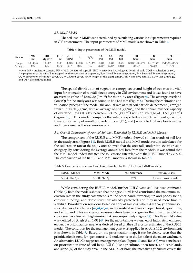
The soil loss in MMF was determined by calculating various input parameters requiredin GIS environment. The input parameters of MMF models are shown in Table 4.

Table 4. Input parameters of the MMF model.

Factors MS(m)

BD(Mg m−3)

EHD(m)

COH(KPa) A Et/Eo

CC(%)

GC(%)

PH(m)

ER(mm)

LD(mm)

DT(mm)

Range 0.08–0.45 1.2–1.7 7–15 0–105 0–0.35 0.05–0.9 0–70 0–70 0–25 1718.71–2645.71 0–1851.77 2645.41–515.62Average 0.25 1.32 11.57 70.59 0.25 0.5 36.87 36.87 23.88 1838.08 676.62 1165.60

where MS = moisture content, BD = bulk density of topsoil, EHD = effective hydrological depth of soil, COH = cohesion of soil,A = proportion of the rainfall intercepted by the vegetation or crop cover, Et = Actual Evapotranspiration, E0 = Potential Evapotranspiration,CC = proportion of canopy cover, GC = Ground cover, PH = height of the plant canopy, ER = effective rainfall, LD = leaf drainage,and DT = direct through fall.

The spatial distribution of vegetation canopy cover and height of tree was the vitalinput for estimation of rainfall kinetic energy in GIS environment and it was found to havean average value of 40402.80 (J m−2) for the study area (Figure 9). The average overlandflow (Q) for the study area was found to be 64.66 mm (Figure 8). During the calibration andvalidation process of the model, the annual rate of total soil particle detachment (J) rangedfrom 5.15–15.50 (kg/m2) with an average of 5.53 (kg/m2), and the annual transport capacityof overland flow (TC) lay between 0–35.72 (kg/m2) with an average of 11.50 (kg/m2)(Figure 10). This model compares the rate of expected splash detachment (J) with atransport capacity of runoff or overland flow (TC), and J was noted to have lower valuesand it was used as the soil erosion rate.

3.4. Overall Comparison of Annual Soil Loss Estimated by RUSLE and MMF Models

The comparison of the RUSLE and MMF models showed similar trends of soil lossin the study area (Figure 11). Both RUSLE model and MMF model results calculated forthe soil erosion rate at the study area showed that the area falls under the severe erosioncategory. By considering the average annual soil loss from the models, it was found thatthe MMF model underestimated the soil erosion rate relative to the RUSLE model by 7.72%.The comparison of the RUSLE and MMF models is shown in Table 5.

Table 5. Comparison of annual soil loss estimated by the RUSLE and MMF models.

RUSLE Model MMF Model % Difference Erosion Class

59.94 t/ha/yr 55.30 t/ha/yr 7.74 Severe erosion risk

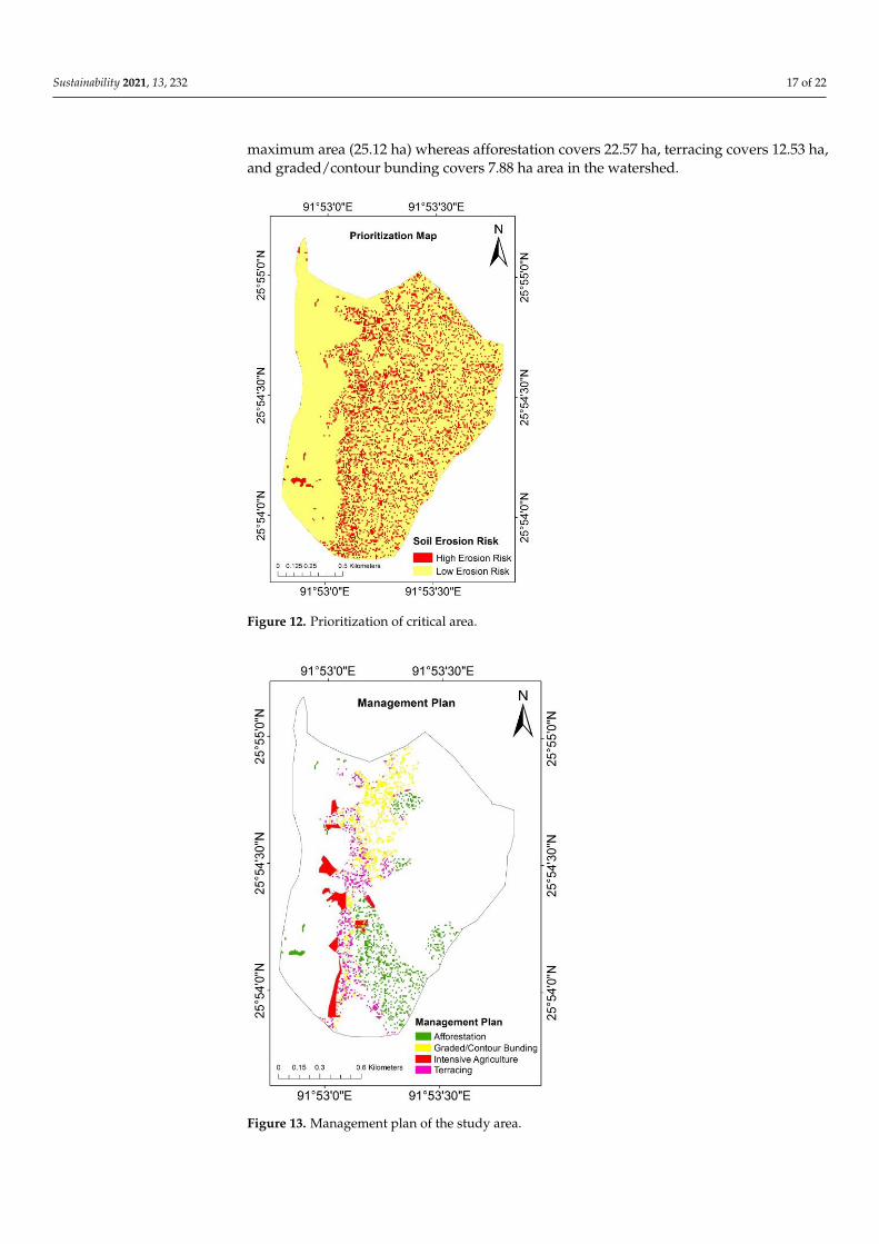
While considering the RUSLE model, further LULC wise soil loss was estimated(Table 6). Both the models showed that the agricultural land contributed the maximum soilerosion rate in the study catchment. On the other hand, terracing, upland paddy fields,contour bunding, and dense forest are already protected, and they need more time tostabilize. Prioritization was done based on annual soil loss, where 40 t/ha/yr annual soilwas taken as a benchmark [42,44,46,47] in the unsterilized areas of open forest, agriculture,and scrubland. This implies soil erosion values lesser and greater than this threshold areconsidered as a low and high erosion risk area respectively (Figure 12). This threshold valuewas defined by Singh et al. 1992 [47] for the mountainous watershed of India. As mentionedearlier, the prioritization map was derived based on the soil erosion estimates of the RUSLEmodel. The condition for the management plan was applied in ArcGIS 10.2 environment;it is shown in Table 7. Based on the prioritization map, it can be clearly seen that theprioritization is none for open forests and settlements on the left side of the micro-catchment.An alternative LULC/suggested management plan (Figure 13 and Table 8) was done basedon prioritization (rate of soil loss), LULC (like agriculture, open forest, and scrubland),and slope (%) of the study area. In the ALULC or BMP, the intensive agriculture covers the

Sustainability 2021, 13, 232 17 of 22

maximum area (25.12 ha) whereas afforestation covers 22.57 ha, terracing covers 12.53 ha,and graded/contour bunding covers 7.88 ha area in the watershed.

Sustainability 2020, 12, x FOR PEER REVIEW 17 of 22

Figure 12. Prioritization of critical area.

Figure 13. Management plan of the study area.

Figure 12. Prioritization of critical area.

Sustainability 2020, 12, x FOR PEER REVIEW 17 of 22

Figure 12. Prioritization of critical area.

Figure 13. Management plan of the study area. Figure 13. Management plan of the study area.

Sustainability 2021, 13, 232 18 of 22

Table 6. LULC wise soil loss estimated at the study area.

LULC AverageSoil Loss (t/ha/yr) Erosion Area (ha) Total Area (ha) % Area

Agriculture 79.10 23.83 44.29 53.80Dense forest 53.76 26.45 78.8 33.57Open forest 46.39 23.45 55.15 42.52Scrubland 62.67 19.26 49.37 39.01Terracing 0.00 0.00 0.19 0.00

Upland paddy field 15.50 3.00 8.86 33.86Contour bunding 0.00 0.00 4.20 0.00

Table 7. Condition for management plan.

Soil Loss (t ha−1 yr-−1) >40 >40 >40 <40

% slope 0–8 8–33 >33 0–8

LULCAgriculture Agriculture Agriculture AgricultureOpen forest Open ForestScrubland Scrubland Scrubland

Management plan Graded/contour bunding Terracing Afforestation Intensive agriculture

Table 8. Management plan of the prioritized area.

Management Plan

LULC Graded/ContourBunding (ha) Afforestation (ha) Intensive

Agriculture (ha) Terracing (ha) Total Area (ha)

Agriculture 7.50 - 25.12 4.19 36.81Open Forest 0.04 10.26 - - 10.31Scrubland 0.34 12.31 - 8.34 20.99

Total Area (ha) 7.88 22.57 25.12 12.53 68.01

4. Discussion

The study area is situated in mountainous regions of India which faces a major problemof soil erosion as is presented in this study. This problem occurs due to high and erraticrainfall [48,49], higher value of soil erodibility, slope length, and crop management factor(as identified in this study). Additionally, little to no conservation practices (terracing andcontouring) have been employed in the study area which has led to the high soil erosion.As the watershed is mountainous with a steep slope, it inherits a high slope length factorand consequently high overland flow with high velocity. Slope length is the primary factorinfluencing soil erosion [50,51] and its impact is complex [52]. As the slope length increases,this leads to the high overland flow and results in the increase in soil erosion and sedimentyield in the study area. High rainfall erosivity (R) was found in the study. A higher R valueindicates higher kinetic energy of rainfall and surface runoff, which contributes to highersoil erosion [53]. Moreover, the high soil erodibility factor (K) directly increased the rate ofsoil erosion [33,37,54]. The predicted soil erosion for the study area was close to the otherstudies in India and other countries’ hilly watersheds [54–56]. Soil erosion leads to loss ofsoil nutrients and a decrease in soil fertility that should give significant attention duringthe construction of the conservation management plan [57]. Based on soil loss and landuse, the watershed is prioritized for conservation measures. The management plan for soilconservation and watershed development by reducing soil loss was made based on theslope, LULC, and soil loss classes. High soil erosion was found from the agricultural landand the management plans were prepared accordingly. For this, a change in the existingagricultural cultivation system should be done with intensive agriculture, contour bunding,and terracing. The conservation structures restrict soil erosion by reducing the overland

Sustainability 2021, 13, 232 19 of 22

flow. The contour bunding and terracing reduce the slope length and also increase theinfiltration capacity of the soil.

Prior to the comparison of the RUSLE and MMF models, both models were calibrated(2010–2015) and validated (2016–2019) against observed soil loss (measured at the catch-ment outlet). The model parameters were adjusted manually during model calibration.Two model parameters (α and β) and one model parameter (plant height) were usedin model calibration for the RUSLE and MMF models, respectively. While α and β pa-rameters relate NDVI and the C factor, they are sensitive to land use type. Throughoutthe study catchment, α and β parameters varied with an average value of 2.06 and 0.97,respectively. Similarly, the plant height parameter in MMF model varied spatially dueto different land use types across the catchment. As displayed in Figure 5, the calibratedvalues for different land use types ranged from 0 (for water body) to 23.54 (dense forest).These calibrated values (both RUSLE and MMF model parameters) were used in modelvalidation for the year 2016–2019, where the model simulated soil erosion was comparedagainst the observed soil loss. The results demonstrated NSE, MAE and RMSE valuesof 0.73, 0.95 t/ha/yr, 1.51 t/ha/yr, and 0.71, 3.69 t/ha/yr, 3.85 t/ha/yr for RUSLE andMMF models, respectively, during model validation (Table 3). These results indicate thatboth models are well in agreement with the observed soil loss in the study catchment withminor superior performance observed for the RUSLE model.

With regards to the BMP strategies to combat the soil erosion within the micro-catchment, RUSLE method was used to identify the prioritization areas within the catch-ment. The prioritization plot (Figure 12) displays the priority areas are more dominantin the right-hand side of the catchment which is predominantly dense forest, scrubland,agriculture, contour bunding, and upland paddy field types of LULC. The suggestedmanagement plan (Figure 13) showcases that afforestation is mainly suggested for the openforest LULC, contour bunding is recommended for agricultural LULC within steep slopes,and terracing is suggested for both agricultural lands as well as scrublands (dependingon slopes). Table 7 displays the total area under agricultural LULC suggested for contourbunding and terracing are 7.50 ha and 4.19 ha, respectively. Similarly, for open forest LULC,contour bunding and afforestation are suggested for 0.04 ha and 10.26 ha, respectively.On the other hand, for scrubland LULC, 0.34 ha, 12.31 ha, and 8.34 ha land area are sug-gested for contour bunding, afforestation, and terracing, respectively. This indicates that asignificant area is under severe erosion in case of scrubland which requires afforestation.Nevertheless, proper management practices are paramount in the study micro-catchmentfor reducing soil loss irrespective of the LULC.

A similar study was done using RUSLE model at West Bengal, India [58] for alike landuse class of this study and found an increase in the rate of erosion with increasing areas indense forests (134 t/ ha/yr, 55 km2), degraded forests (169 t/ha/yr, 137 km2), and settlementareas (30 t/ ha/yr, 105 km2), which is closely in line with our results. Furthermore, severalother studies at different geographic domains (mountainous and plain) of India such as in theUrmodi river watershed at Maharashtra, India with an area of 70.22 km2, found areas to beunder very severe erosion risk (>80 t/ha/yr) [59]. In another watershed (Konar river basin),using RUSLE, the soil loss was found to be in the very high category of 5–40 t/ha/yr [60].Synonymously, studies on similar slope and land use catchments in countries like Sri Lanka,Malaysia, and Rwanda also revealed high rate of soil erosion [55,61,62]. Moreover, in Rwanda,91% of the study area comprised of slope more than 15◦ and the average soil loss wasin the range of 31–41 t/ha/yr [55], which is consistent with this study since 60% of thearea is comprised of high slope (>25◦) and falls under severe erosion classes (>40 t/ha/yr).The present study enabled us to prioritize the different segments of watershed based onsoil erosion risk. This will help in proper land uses and planning conservation practices inthe future extension of agricultural activities. The alternate land uses for the watershed areexpected to be followed by the farming communities to achieve sustainability in agriculturalproductions. The results from the study will help in understanding the erosion risk ofwatershed vis-à-vis land uses so that the same can be extrapolated to other watersheds with

Sustainability 2021, 13, 232 20 of 22

similar landforms, soil, and land use. These findings from other studies are in line with thefindings of this study, which indicates the wide applicability of these soil erosion models inlarger catchment sizes. This study on the other hand indicates the applicability for smallersized catchment as well for evaluating BMPs.

5. Conclusions

The average annual soil erosion estimated with RUSLE was found to be 59.94 t/ha/yr,whereas the MMF model estimated soil loss as 55.30 t/ha/yr. Since there was an absolutedifference of only 7.74%, the estimates made by both the models can be considered at par.At this range of soil loss, the watershed can be classified as a severely eroded catchmentand it needs suitable land use management plans to combat the severe soil erosion. The soilerosion was found to be highest in the agriculture dominated area (79.10 t/ha/yr), followedby scrubland (62.67 t/ha/yr). Under the alternative management plan, considering thethreshold of 40 t/ha/yr, intensive agriculture is suggested only in those areas havinga slope less than 8%. Within the study watershed, 68.01 ha area is prioritized for soilconservation measures to reduce the erosion potential under proposed alternative landuses. The results from the study will help in understanding the erosion risk of watershedvis-à-vis land uses so that the same can be extrapolated to other watersheds with similarlandforms, soil, and land uses. These findings will aid in implementing robust BMPs in thehilly and mountainous regions in the world.

Author Contributions: S.D. conducted the study with suggestions from P.K.B. and S.D.; P.K.B.and P.D. wrote the original and the revised manuscript; and P.K. reviewed and commented on theoriginal draft of the manuscript. All authors have read and agreed to the published version ofthe manuscript.

Funding: This research received no external funding.

Institutional Review Board Statement: The study was the partial fulfilment of Post Graduate (PG)degree work of Susanta Das and it was approved by the Indira Gandhi Krishi Vishwavidyalayaresearch committee in 2017.

Informed Consent Statement: Not applicable.

Data Availability Statement: The data presented in this study are available on request from thecorresponding author. The data are not publicly available since they are collected by the first authorof this paper.

Acknowledgments: The authors would like to acknowledge Er Ranjit Das of North Eastern SpaceApplications Centre (NESAC), Umiam, Meghalaya, India and M.P. Tripathi of Indira Gandhi KrishiVishwavidyalaya, Raipur, Chhattisgarh, India for their assistance and suggestions while conductingthe study.

Conflicts of Interest: The authors declare no conflict of interest.

References1. Ighodaro, I.D.; Lategan, F.S.; Yusuf, S.F.G. The impact of soil erosion on agricultural potential and performance of Sheshegu

community farmers in the Eastern Cape of South Africa. J. Agric. Sci. 2013, 5, 140–147. [CrossRef]2. Koirala, P.; Thakuri, S.; Joshi, S.; Chauhan, R. Estimation of Soil Erosion in Nepal Using a RUSLE Modelling and Geospatial Tool.

Geoscience 2019, 9, 147. [CrossRef]3. Lal, R.; Singh, B.R. Effects of Soil Degradation on Crop Productivity in East Africa. J. Sustain. Agric. 1998, 13, 15–36. [CrossRef]4. Hategekimana, Y.; Allam, M.; Meng, O.; Nie, Y.; Mohamed, E. Quantification of Soil Losses along the Coastal Protected Areas in

Kenya. Land 2020, 9, 137. [CrossRef]5. Claessens, L.; Van Breuge, P.; Notenbaert, A.; Herrero, M.; Van De Steeg, J. Mapping potential soil erosion in East Africa using the

Universal Soil Loss Equation and secondary data. IAHS-AISH Publ. 2008, 325, 398–407.6. Ganasri, B.P.; Ramesh, H. Assessment of soil erosion by RUSLE model using remote sensing and GIS—A case study of Nethravathi

Basin. Geosci. Front. 2016, 7, 953–961. [CrossRef]7. Sujatha, E.; Sridhar, V. Spatial Prediction of Erosion Risk of a Small Mountainous Watershed Using RUSLE: A Case-Study of the

Palar Sub-Watershed in Kodaikanal, South India. Water 2018, 10, 1608. [CrossRef]8. Reichmann, O.; Chen, Y.; Iggy, L.M. Spatial model assessment of P transport from soils to waterways in an Eastern Mediterranean

Watershed. Water 2013, 5, 262–279. [CrossRef]

Sustainability 2021, 13, 232 21 of 22

9. Ozsahin, E.; Duru, U.; Eroglu, I. Land use and land cover changes (LULCC), a key to understand soil erosion intensities in theMaritsa Basin. Water 2018, 10, 335. [CrossRef]

10. Deb, P.; Kiem, A.S.; Willgoose, G. A linked surface water-groundwater modelling approach to more realistically simulaterainfall-runoff non-stationarity in semi-arid rgions. J. Hydrol. 2019, 575, 273–291. [CrossRef]

11. Chandra, S.; Manisa, P. Application of RUSLE model for soil loss estimation of Jaipanda watershed, West Bengal. Spat. Inf. Res.2017, 25, 399–409.

12. Woldemariam, G.; Iguala, A.; Tekalign, S.; Reddy, R. Spatial Modeling of Soil Erosion Risk and Its Implication for ConservationPlanning: The Case of the Gobele Watershed, East Hararghe Zone, Ethiopia. Land 2018, 7, 25. [CrossRef]

13. Reitsma, K.D.; Dunn, B.H.; Mishra, U.; Clay, S.A.; DeSutter, T.; Clay, D.E. Land-use change impact on soil sustainability in aclimate and vegetation transition zone. Agron. J. 2015, 107, 2363–2372. [CrossRef]

14. Perez-Molina, E.; Sliuzas, R.; Flacke, J.; Jetten, V. Developing a cellular automata model of urban growth to inform spatial policyfor flood mitigation: A case study in Kampala, Uganda. Comput. Environ. Urban Syst. 2017, 65, 53–65. [CrossRef]

15. Pelacani, S.; Marker, M.; Rodolfi, G. Simulation of soil erosion and deposition in a changing land use: A modelling approach toimplement the support practice factor. Geomorphology 2008, 99, 329–340. [CrossRef]

16. Wischmeier, W.H.; Smith, D.D. Predicting Rainfall Erosion Losses from Cropland East of the Rocky Mountains; U. S. Dept. of Agric. AH,282.U.S.; Government Printing Office: Washington, DC, USA, 1965.

17. Morgan, R.P.C.; Morgan, D.D.V.; Finney, H.J. A predictive model for the assessment of erosion risk. J. Agric. Eng. Res. 1984,30, 245–253. [CrossRef]

18. Renard, K.G.; Foster, G.R.; Weesies, G.A.; Porter, J.P. RUSLE: Revised universal soil loss equation. J. Soil Water Conserv. 1991,46, 30–33.

19. Mendoza-ponce, A.; Corona-núñez, R.; Kraxner, F.; Leduc, S.; Patrizio, P. Identifying effects of land use cover changes and climatechange on terrestrial ecosystems and carbon stocks in Mexico. Glob. Environ. Chang. 2018, 53, 12–23. [CrossRef]

20. Alphan, H.; Derse, M.A. Change detection in Southern Turkey using normalized di_erence vegetation index (NDVI). J. Environ.Eng. Landsc. Manag. 2013, 21, 12–18. [CrossRef]

21. Moran-Tejeda, E.; Zabalza, J.; Rahman, K.; Gago-Silva, A.; López-Moreno, J.I.; Vicente-Serrano, S.; Lehmann, A.; Tague, C.L.;Beniston, M. Hydrological impacts of climate and land-use changes in a mountain watershed: Uncertainty estimation based onmodel comparison. ECO Hydrol. 2014, 8, 1396–1416. [CrossRef]

22. Taye, G.; Vanmaercke, M.; Poesen, J.; Van Wesemael, B.; Tesfaye, S.; Teka, D.; Nyssen, J.; Deckers, J.; Haregeweyn, N. DeterminingRUSLE P- and C-factors for stone bunds and trenches in rangeland and cropland, North Ethiopia. L. Degrad. Dev. 2018,29, 812–824. [CrossRef]

23. Zeng, C.; Wang, S.; Bai, X.; Li, Y.; Tian, Y.; Li, Y.; Wu, L.; Luo, G. Soil erosion evolution and spatial correlation analysis in a typicalkarst geomorphology using RUSLE with GIS. Solid Earth 2017, 8, 721–736. [CrossRef]

24. Lazzari, M.; Gioia, D.; Piccarreta, M.; Danese, M.; Lanorte, A. Sediment yield and erosion rate estimation in the mountaincatchments of the Camastra artificial reservoir (Southern Italy): A comparison between different empirical methods. Catena 2015,127, 323–339. [CrossRef]

25. Dimotta, A.; Lazzari, M.; Cozzi, M.; Romano, S. Soil Erosion Modelling on Arable Lands and Soil Types in Basilicata, Southern Italy;Gervasi, O., Ed.; ICCSA 2017, Part V, Lecture Notes in Computer Science LNCS; Springer: Cham, Switzerland, 2017; Volume 10408,pp. 57–72.

26. Meyer, L.; Wischmeier, W. Mathematical simulation of the process of soil erosion by water. Trans. ASAE 1969, 12, 754–758.27. Wischmeier, W.H.; Smith, D.D. Predicting Rainfall Erosion Losses—A Guide to Conservation Planning; AH-537; U.S. Department of

Agriculture: Beltsville, MD, USA, 1978.28. Morgan, R.P.C. Soil Erosion and Conservation, 3rd edition. Eur. J. Soil Sci. 2005, 56, 681–687.29. Ghosh, S.; Guchhait, S.K. Soil loss estimation through USLE and MMF methods in the Lateritic Tracts of Eastern Plateau Fringe of

Rajmahal Traps, India. Ethiop. J. Environ. Stud. Manag. 2012, 5, 529–541. [CrossRef]30. Deb, P.; Kiem, A.S. Evaluation of rainfall-runoff model performance under non-stationary hydroclimatic conditions. Hydrol. Sci. J.

2020, 65, 1667–1684. [CrossRef]31. Behera, R.N.; Nayak, D.K.; Andersen, P.; Måren, I.E. From jhum to broom: Agricultural land-use change and food security

implications on the Meghalaya Plateau, India. Ambio 2015, 45, 63–77. [CrossRef]32. Saha, R.; Chaudhary, R.S.; Somasundaram, J. Soil Health Management under Hill Agroecosystem of North East India.

Appl. Environ. Soil Sci. 2012, 2012, 696174. [CrossRef]33. Das, S.; Bora, P.K.; Katre, P. Determining and Mapping of Soil Erodibility Index for Nongpoh Watershed. Indian J. Hill Farming

2019, 32, 27–33.34. Lee, S. Geological application of geographic information system. Korea Inst. Geosci. Min. Resour. 2014, 9, 109–118.35. Silalahi, F.E.S.; Pamela, A.Y.; Hidayat, F. Landslide susceptibility assessment using frequency ratio model in Bogor, West Java,

Indonesia. Geosci. Lett. 2019, 6, 10. [CrossRef]36. Olaniya, M.; Bora, P.K.; Das, S.; Chanu, P.H. Soil erodibility indices under different land uses in Ri-Bhoi district of Meghalaya

(India). Sci. Rep. 2020, 10, 14986. [CrossRef] [PubMed]37. Das, S.; Sarkar, R.; Bora, P.K. Comparative study of estimation of soil erodibility factor for the lower Transact of Ranikhola

watershed of east Sikkim. J. Plant Develop. Sci. 2018, 10, 317–322.

Sustainability 2021, 13, 232 22 of 22

38. Wischmeier, W.H.; Johnson, C.B.; Cross, B.V. A soil erodibility nomograph for farm-land and construction sites. J. Soil Water Conserv.1971, 26, 189–193.

39. Deb, P.; Debnath, P.; Denis, A.F.; Lepcha, O.T. Variability of soil physicochemical properties at different agroecological zones ofHimalayan region: Sikkim, India. Env. Dev. Sustain. 2019, 21, 2321–2339. [CrossRef]

40. Polykretis, C.; Alexakis, D.D.; Grillakis, M.G.; Manoudakis, S. Assessment of intra-annual and inter-annual variabilities of soilerosion in Crete Island (Greece) by incorporating the dynamic “Nature” of R and C-Factors in RUSLE modeling. Remote Sens.2020, 12, 2439. [CrossRef]

41. Van der Knijff, J.M.; Jones, R.J.A.; Montanarella, L. Soil Erosion Risk Assessment in Europe; EUR 19044 EN; Office for OfficialPublications of the European Communities: Luxembourg, 2000; p. 34.

42. Mondal, A.; Khare, D.; Kundu, S. A comparative study of soil erosion modelling by MMF, USLE and RUSLE. J. Geocarto Int. 2018,33, 89–103. [CrossRef]

43. Dabral, P.P.; Baithuri, N.; Pandey, A. Soil erosion assessment in a hilly catchment of North Eastern India using USLE, GIS andremote sensing. Water Resour. Manag. 2008, 22, 1783–1798. [CrossRef]

44. Srivastava, R.K.; Sharma, H.C.; Raina, A.K. Suitability of soil and water conservation measures for watershed management usinggeographical information system. J. Soil Water Conserv. 2010, 9, 148–153.

45. Moriasi, D.N.; Arnold, J.G.; Van Liew, M.W.; Bingner, R.L.; Harmel, R.D.; Veith, T.L. Model Evaluation Guidelines for SystematicQuantification of Accuracy in Watershed Simulations. Trans. ASABE 2007, 50, 885–900. [CrossRef]

46. Pandey, A.; Mathur, A.; Mishra, S.K.; Mal, B.C. Soil erosion modeling of a Himalayan watershed using RS and GIS.Environ. Earth Sci. 2009, 59, 399–410. [CrossRef]

47. Singh, G.; Babu, R.; Narain, P.; Bhushan, L.S.; Abrol, I.P. Soil erosion rates in India. J. Soil Soil Water Conserv. 1992, 47, 97–99.48. Yadav, S.; Deb, P.; Kumar, S.; Pandey, V.; Pandey, P.K. Trends in major and minor meteorological variables and their influence on

reference evapotranspiration for mid Himalayan region at east Sikkim, India. J. Mt. Sci. 2016, 13, 302–315. [CrossRef]49. Marak, J.D.; Sarma, A.K.; Bhattacharjya, R.K. Innovative trend analysis of spatial and temporal rainfall variations in Umiam and

Umatru watersheds in Meghalaya, India. Theor. Appl. Climatol. 2020, 142, 1397–1412. [CrossRef]50. Wilkinson, M.T.; Humphreys, G.S. Slope aspect, slope length and slope inclination controls of shallow soils vegetated by

sclerophyllous heath—Links to long-term landscape evolution. Geomorphology 2006, 76, 347–362. [CrossRef]51. Liu, B.Y.; Nearing, M.A.; Shi, P.J.; Jia, Z.W. Slope length effects on soil loss for steep slopes. Soil Sci. Soc. Am. J. 2000, 64, 1759–1763.

[CrossRef]52. Han, Z.; Zhong, S.; Ni, J.; Shi, Z.; Wei, C. Define the Slope Length of Newly Reconstructed Gentle-Slope Lands in Hilly

Mountainous Regions. Sci. Rep. 2019, 9, 4676. [CrossRef]53. Balasubramani, K.; Gomathi, M.; Bhaskaran, G.; Kumaraswamy, K. GIS-based spatial multi-criteria approach for characterization

and prioritization of micro-watersheds: A case study of semi-arid watershed, South India. Appl. Geomat. 2019, 11, 289–307.[CrossRef]

54. Pal, S.C.; Chakrabortty, R. Simulating the Impact of Climate Change on Soil Erosion in Sub-Tropical Monsoon DominatedWatershed Based on RUSLE, SCS Runoff and MIROC5 Climatic Model. Adv. Space Res. 2019, 64, 352–377. [CrossRef]

55. Dissanayake, D.; Morimoto, T.; Ranagalage, M. Accessing the soil erosion rate based on RUSLE model for sustainable land usemanagement: A case study of the Kotmale watershed, Sri Lanka. Modeling Earth Syst. Environ. 2018, 5, 291–306. [CrossRef]

56. Ostovari, Y.; Moosavi, A.A.; Pourghasemi, H.R. Soil loss tolerance in calcareous soils of a semi-arid region: Its evaluation,prediction, and influential parameters. Land Degrad. Develop. 2020, 31, 2156–2167. [CrossRef]

57. Shen, Z.Y.; Gong, Y.W.; Li, Y.H.; Liu, R.M. Analysis and modeling of soil conservation measures in the Three Gorges ReservoirArea in China. Catena 2010, 81, 104–112. [CrossRef]

58. Bhattacharya, R.K.; Das Chatterjee, N.; Das, K. Land use and land cover change and its resultant erosion susceptible level:An appraisal using RUSLE and Logistic Regression in a tropical plateau basin of West Bengal, India. Environ. Dev. Sustain.2020, 1–36. [CrossRef]

59. Bagwan, W.A.; Gavali, R.S. Delineating changes in soil erosion risk zones using RUSLE model based on confusion matrix for theUrmodi river watershed, Maharashtra, India. Modeling Earth Syst. Environ. 2020, 1–14. [CrossRef]

60. Rajbanshi, J.; Bhattacharya, S. Assessment of soil erosion, sediment yield and basin specific controlling factors using RUSLE-SDRand PLSR approach in Konar river basin, India. J. Hydrol. 2020, 587, 124935. [CrossRef]

61. Islam, M.R.; Jaafar, W.Z.W.; Hin, L.S.; Osman, N.; Karim, M.R. Development of an erosion model for Langat River Basin, Malaysia,adapting GIS and RS in RUSLE. Appl. Water Sci. 2020, 10, 1–11. [CrossRef]

62. Byizigiro, R.V.; Rwanyiziri, G.; Mugabowindekwe, M.; Kagoyire, C.; Biryabarema, M. Estimation of Soil Erosion Using RUSLEModel and GIS: The Case of Satinskyi Catchment, Western Rwanda. Rwanda J. Eng. Sci. Technol. Environ. 2020, 3. [CrossRef]