Design and Implementation of Path Trackers for Ackermann

Design and Implementation of Path Trackersfor Ackermann Drive based Vehicles

Adarsh Patnaik*a Manthan Patel*a Vibhakar Mohta*a Het Shah*a Shubh Agrawal*a Aditya Rathore*b

Ritwik Malik*c Debashish Chakravartyc Ranjan Bhattacharyaa

Abstract—This article is an overview of the variousliterature on path tracking methods and their implemen-tation in simulation and realistic operating environments.The scope of this study includes analysis, implementation,tuning, and comparison of some selected path trackingmethods commonly used in practice for trajectory trackingin autonomous vehicles. Many of these methods are appli-cable at low speed due to the linear assumption for thesystem model, and hence, some methods are also includedthat consider non-linearities present in lateral vehicledynamics during high-speed navigation. The performanceevaluation and comparison of tracking methods are carriedout on realistic simulations and a dedicated instrumentedpassenger car, Mahindra e2o, to get a performance ideaof all the methods in realistic operating conditions anddevelop tuning methodologies for each of the methods. Ithas been observed that our model predictive control-basedapproach is able to perform better compared to the othersin medium velocity ranges.Keywords: Path Tracking, Control Systems, State-SpaceModel, State Estimation, Autonomous Navigation.

I. INTRODUCTION

In past years, the development in the area of au-tonomous vehicles has been stupendous through techno-logical advances made in the areas of communication,computing, sensors, and electronic devices along withadvanced processing algorithms. In this section, wediscuss the importance and literature review of imple-menting an autonomous system module, path tracker,that is necessary for accurate and safe manoeuvring ofan autonomous vehicle. It is required for the properfunctioning of modules like collision avoidance, lateraland longitudinal motion control.

Precise path following by a car-like robot is only pos-sible if it is able to follow the desired steering angle anddesired velocity at each time step during the traversal.A club of all such vehicle controllers is scientificallytermed as path trackers. The expected goal of a pathtracking algorithm is to generate actuator commandsthat minimize the cross-track error or simply the lateral

* Denotes Equal Contributiona Department of Mechanical Engineering, IIT Kharagpurb Department of Electrical Engineering, IIT Kharagpurc Department of Mining Engineering, IIT Kharagpur

distance between the vehicle’s center point and the geo-metric path estimated by the motion planner. Apart fromthis, it is also expected that the controller minimizes thedifference between the vehicle’s orientation and path’sheading while also limiting the rate of steering input foroverall lateral stability and smooth driving experience.Path tracking controllers have been existing since theadvent of autonomous vehicles and recent developmentshave made them very extensive and robust to systemassumptions.

For each of the controller presented in this work,its theory with system model is discussed first beforeimplementation of the controller itself. To ease com-parison based study, we limit the performance tuningparameters and analyze the performance of trackers onfour different types of courses. Rest of this work isdivided as follows. Section III describes the experimentalsetup used for simulation, various courses designed foranalysis and computational platform used for carryingout the experiments. Path tracking algorithm, in general,can be defined as a combination of two control systems,i.e., lateral control and longitudinal control of the vehi-cle. Section IV presents the development of longitudinalcontrol of the vehicle, which is a pre-requisite for lateralcontrol to perform at its best. This section introducestwo types of velocity controller commonly found inindustry, i.e., PID and Adaptive PID controller, and theircomparison before selecting one as the base longitudinalcontroller for our lateral control study. Section V thenpresents the complete study of lateral control startingfrom introduction to different vehicle driver models,then discusses the synthesis of commonly found lateralcontrol theory in practice before finally discussing theiranalysis and head-to-head performance comparison. Theexperiments carried out in sections IV, and V is carriedwithin a computer simulation for quick prototyping ofthe complete control system framework before using thesame framework on our real passenger car. Section VIthen presents some of the pre-requisite experimentationneeded on the passenger car and finally discusses theresults of complete path tracking implementation. Ul-timately, section VII concludes the presented work, inbrief, its importance and illustrates how commonly usedprimitive control techniques are used successfully. It also

arX

iv:2

012.

0297

8v1

[cs

.RO

] 5

Dec

202

0

discusses the need for developing more advanced pathtracking theories as autonomous vehicles are moving to-wards high-speed operations and complicated objectives.

II. LITERATURE REVIEW

The importance of path tracking systems has alreadybeen discussed in the previous section. Two importantsurvey papers [1], [2] have been published so far thatdiscusses the merits and demerits of various controllersdeveloped in this domain. [1] has classified the pathtracking systems into three approaches viz. Geomet-ric model-based, Kinematic model-based, and Dynamicmodel-based approaches. The geometric model revolvesaround tracking capability only by involving geometryof the vehicle(s) and path(s). Though this method seemsnaive, it was a core component of winning team’svehicle in DARPA grand challenge in the year 2004[3]. The kinematic model discussed in this work derivesan approximate kinematic bicycle model equivalent tothe car, on which controllers were developed. Further,a dynamic model for the vehicle is also developedfor incorporating the vehicle dynamics for enhancedprecision tracking in high-speed navigation. [2] havediscussed motion planning along with the path controlapproaches adjunctly as they mention that both of thesefields to be closely related. They have divided the pathtracking systems based on control objective, either pathstabilization or trajectory stabilization. Similar to thekinematic model approximation, this work has explaineddifferent approaches separately as path stabilization us-ing the kinematic model and trajectory stabilization usingthe kinematic model. This study has also discussedthe application of predictive control approaches andparameter varying controllers as modern techniques totackle the path tracking problem.

One of the most famous geometric model controller,the pure pursuit algorithm [4] was originally developedas a process for calculating the local path to get a robotback to the global path. Terragator, a six-wheeled skidsteered robot used for outdoor vision experiments wasthe first application of this method. Modeling and controlfor a three wheeled mobile robot has been presented in[5]. Some of the studies, like the one done by [6] alreadyhave pointed out the problem with this tracker. Thatis, it faces problems like corner-cutting and significantsteady-state error if an appropriate look-ahead distanceis not selected, especially at higher speeds(greater than30 kmph). Another famous geometric model, Stanleymethod [3], is known to perform better than pure pur-suit by avoiding corner-cutting and reducing steady-state error. It estimates the steering angle based on anonlinear control law that considers the heading errorof vehicle with respect to the path as well as the cross-track error that is measured from the front axle of the

vehicle to the path. It is further shown that it has ahigher tendency for oscillation and is not as robustto discontinuity in the path as compared to the purepursuit method. In the past, researchers have also comeup with a modified version of these geometric modelslike [6], [7], [8], [9] that focused on eradicating thecons of the mentioned methods. Feedback methods arealso a plausible replacement to the geometric modelsas they are more robust to external disturbances andinitial errors. An interesting method for controlling thekinematic model of non-holonomic systems (car-likerobot) is discussed in [10]. This study derived a kine-matic model of a car-like robot along with the feedbackcontrol law, which can also be easily extended to control’n’ trailers attached to the system. However, at higherspeeds, this model too gives significant cross track erroras it neglects the vehicle’s lateral dynamics. At this level,the vehicle dynamics are considerably sophisticated, andhigh fidelity models are quite nonlinear, time-taking andvary with changing environments. Their negligence invehicle system modeling leads to increased cross-trackerror in high-speed navigation. This has been very wellinvestigated in the studies made by [11], [12]. Theyhave also devised an Linear Quadratic Regulator(LQR)method that utilizes the inclusion of the lateral dynamicsinto the state-space model and gives fairly better resultsthan the geometric and kinematic models. However,these methods include an approximate linearized vehicledynamics and thus leaves a scope of improvement.Model predictive control [13] is known to be a generalcontrol design methodology which can be easily ex-tended to path tracking problem. Intuitively, the approachis to resolve the motion planning problem over a shortperiod horizon, then take a small time frame windowof the output open-loop control, and apply it to thevehicle system. Like discussed in the previous section,the availability of high-end computational devices hasmade the computation of predictive control algorithmfeasible in real-time and comfortable for use on-boardvehicle. Some variations of model predictive controlframework that are found in past literature include a)Unconstrained Model Predictive Control (MPC) withKinematic Models [14], b) Path Tracking Controllers[15], c) Trajectory Tracking Controllers [16].

III. SIMULATION SETUP AND VEHICLE PLATFORM

This work is focused towards implementation andperformance evaluation of different path trackers, andhence, a typical experimental setup is necessary to min-imize any error/bias induced by variation in hardwaresetup or software framework. Sufficient time was spenton choosing these platforms that are compliant withthe academic literature and are also commonly used inindustry to confirm for their usage reliability.

2

A. MATLAB for Plant and Controller analysis

Before implementing any of the path trackers, it isbest to undertake some analysis on the model for itsstability check and system behavior. We chose MATLABControl Toolbox for the analysis of the models due toit’s accurate results and it’s easy interface. We wereable to specify the path tracking controller as a transferfunction, state-space, or frequency-response model. Thetoolbox also helped in tuning the SISO and MIMOcompensators, like the PID based tracker and LQR basedtracker. Validation of the design by verifying overshoot,settling time, rise time, and phase margins was alsoquick using this platform. Since we were not able tofind any satisfactory resources using which, we couldassemble the controller model defined in MATLAB witha car or could model the car-environment interaction, thisplatform remained useful only for mathematical analysisand observations.

B. Simulation world setup

(a) Simulation’s planned urbanscenario

(b) Simulation’s vehicle for con-ducting experiments

Fig. 1: OSRF Car Simulator screenshot

Before testing the algorithms on some hardware, itis preferred to test in a simulation environment. Wechose Gazebo with the Robot Operating System (ROS)as backend as it is widely used as a simulation stackin the robotics research community. There exist variouspackages pre-compiled that control the robots so thatwe focus towards only the module of our interest, in ourcase, path tracking. For our purpose, we were able tofind a simulation world that included a car and urbanenvironment, just enough to satisfy the requirements.This simulation software released by OSRF realisticallymodels various parameters of the car and its interactionwith the surrounding environment quite similar to thereal-world scenario. Figure 1 is a screenshot of car_demoanimation. The controller programs were implementedusing Python and C++ language, and they communicatewith this simulator at a high rate with a visualizationwindow that helps in investigating their performances.

All the demonstrated experiments viz. analysis usingMATLAB and controller performance in the simulationworld were carried out on an Intel Core i5 @1.7 GHz x2 machine loaded with 8 GB RAM and Ge-Force 820MGPU running Ubuntu 16.04 OS.

All of the trackers were to be tested on some pre-determined paths. Rather than having them tested on arandom driving course, they were validated against somespecific geometry of paths to provide insights into theirrelative advantages and disadvantages in an organizedmanner. Figure 2 shows a pictorial representation of thedefined courses.

(a) Straight line course (b) Circular course

(c) Lane shift course (d) Sinusoidal course

Fig. 2: Courses used for validating path tracking capa-bilities

1) Straight line course: This is the most straight-forward course for the vehicle to follow. This coursebasically validates if the vehicle can maneuver a givenpath without much attention given to tuning of parame-ters. Once the vehicle is fine-tuned, the maneuver on astraight-line path can give expectation value of minimalcross-track, settling time, and peak cross-track error. Thistrack was performed with constant velocities of 10 kmph,20 kmph and 35 kmph indicating slow, medium, andhigh-speed scenarios respectively.

2) Lane shift course: The lane shift course is ascenario in which the vehicle is expected to perform asimple lane change procedure. This course is a standardtest for a vehicle undergoing lane change on a highwayor a collision avoidance scenario. It is also chosen todemonstrate the tracking capability as well as responseto an instantaneous, continuous section. Maneuvers onthis course were also carried at constant velocities of10 kmph, 20 kmph and 35 kmph similar to the cruisecontrol of the vehicle on a highway.

3) Circular course: This course consists of a circularpath of a constant radius (higher than the vehicle’s mini-mum turning radius). It can be related to a roundabout inan urban driving scenario near the square. Interestingly,this course can provide valuable insight into the control

3

of vehicle like the steady-state characteristics whilemaneuvering a constant non-zero curvature path likethis. Experiments on this course were carried at constantvelocities of 10 kmph, 20 kmph and 35 kmph like theprevious courses.

4) Sinusoidal course: This course consists of a si-nusoidal curve-shaped path, which is usually difficultto encounter in an urban driving scenario. The mainhighlight of this course is continuously varying curvaturethat changes in both magnitude and sign over the pathlength. It is expected that a controller’s response to thistype of continuous variance provides an insight into itsrobustness and responsiveness. Maneuvers on this coursewere performed at constant velocities of 10 kmph, 20kmph and 35 kmph like the previous courses.

C. Passenger car setup for laboratory-scale deployment

Fig. 3: Vehicle Instrumentation

While the simulator’s physics engine tries its bestto simulate the interaction between the car and theenvironment, there will always be some noisy processesand unmodelled vehicle dynamics. Also, we are able toobserve non-linear mapping which is usually consideredlinear in simulation world like the mapping betweensteering column to actual steering angle, the mappingbetween throttle to vehicle’s acceleration and effect ofunequal loading on the vehicle tires. Hence, we alsoprepare to test out some of the controllers on a dedicatedinstrumented passenger car in real world scenario. Weemployed the passenger car "Mahindra e2o", with CANbased drive by wire system installed for the tests. It ispossible to input steering commands and throttle valueto this vehicle electronically via the CAN bus, whichmakes it easier to use for research purposes. However,a separate driver is needed that allows conversion ofcommands from the USB port of the in-vehicle computerto the CAN bus. We assume it to be predesigned as thedetails of this device driver is not within the scope ofthis study.

For accurate localization and control signal generation,the test vehicle was equipped with various sensors andcomputation unit. All of the software-based workflowswere performed using an Intel core Xeon @1.7GHz

x 8 machine loaded with 32GB RAM and operatingUbuntu 16.04. IMU, GPS, and rotary encoders providednecessary data for vehicle’s localization whereas KvaserCAN module helped in communicating actuation signalsto the vehicle system. Figure 3 shows overall setup ofdifferent instrumentation.

D. Vehicle LocalizationAccurate localization of the vehicle is necessary to cal-

culate the deviation of the path followed by the vehiclefrom the predetermined path. We resorted to localizationusing the standard method of fusing wheel encoder datawith the IMU data. For this, we utilized the popularrobot_localization package under the ROS frameworkthat internally used an Extended Kalman Filter (EKF) forstate estimation. EKF uses Gaussian noise assumptionfor input sensor signals that improve its ability to dealwith uncertainty while estimating vehicle state. In thiswork, EKF was used to estimate X, Y (current position),and θ (current orientation) given the planar movementassumption of vehicle. After having assembled the rearwheels with rotary encoders and the CG of the vehiclewith IMU, we were able to localize the vehicle usingEKF for sufficiently long distance accurately.

To verify the precise nature of vehicle localizationusing EKF, we carried out a loop closure test forsufficiently long distances. A small orientation or dis-placement error at any point along the loop can showsignificant deviation from the initial position at the endof the test. Figure 4 shows the path trail calculated usingEKF where the change in position error approximates 1.2m for a total traversed the length of 235 m.

Fig. 4: Loop closure given the path traced by vehicle

IV. LONGITUDINAL CONTROL OF VEHICLE

As previously stated, path tracking is a problem ma-jorly focused on lateral control. However, the longitudi-nal velocity does hold importance when a particular pathtracking algorithm uses a velocity term for computingsteering angle. Hence, for completeness, we demonstratethe velocity control capability of the simulated vehicleand realistic vehicle.

4

A. Controller Synthesis

Following methods are chosen based on their simplic-ity and industry-wide acceptance as a control method.The theoretical basis is presented with simplificationusing necessary assumptions.

1) PID Control: Proportional-Integral-DerivativeController (PID Controller) is one of the most popularcontrol loop feedback mechanism for implementingcruise control of a vehicle. For our case, we consideredthe process variable as velocity and the manipulatedvariable as throttle (for both simulated vehicle andrealistic vehicle). Thus, according to PID control theory,the error term e(t), that is a difference between thesetpoint and process variable, controls the throttle ofvehicle proportionally. Figure 5 shows the controllerimplemented for our purpose.

Fig. 5: Illustration of PID velocity controller

Here,a(t) be the throttle input to vehiclev(t) be measured velocity or current velocityr(t) be reference or set pointe(t) be the error signalKp, Ki Kd be the proportional, integral and derivative

gain constants respectivelyFollowing equation was embedded into program forvelocity control,

a(t) = Kpe(t) +Ki

∫e(t)dt+Kde(t) (1)

However, the above equation was converted to discreteform for actual use.

a(t) = Kpe(t)+Ki

t∑0

e(t)+Kde(t)− e(t−∆t)

∆t(2)

where ∆t is the sampling interval used for discretization.• Rise time < 100 ms• Steady-state error < 2%• Overshoot < 10%2) Adaptive PID Control: PID control performs best

when the experimental operating conditions are close tothe tuning operating conditions. Deviations like changein total mass, the slope of the terrain, terrain-wheelinteraction, etc. could make the controller a sub-optimal

performer. These kinds of problems ought to occur inreal-life application of the cruise control. Therefore, thePID constants need to change as a change in operatingconditions occur. We resorted to adaptive PID controllaw, wherein, the constants similar to the ones definedin the previous section can change depending upon theresponse of the controller. One of the popular methodsfor such a self-tuning controller is the MIT rule [17].However, with this method, the system is known to getunstable with time-varying and noisy inputs. Finally, weimplemented a technique that modifies the MIT rule andreduces the risk of instability. Following equations formthe set of rules as explained in the work [18].Here,em(t) be the filter version (low pass first order filer

in this case) of error signal e(t)D(t) be the derivative of error signal e(t)Dm(t) be the derivative of filtered error signal em(t)

Then, the modification in PID constants can be given as,

Kp(k + 1) = Kp(k) + γp|e(k)− em(k)| (3)

Ki(k + 1) = Ki(k) + γiem(k) (4)

Kd(k + 1) = Kd(k) + γd|D(k)−Dm(k)| (5)

where γ is the learning rate for the K constants.

B. Simulation Results and DiscussionMethods described in section IV-A were implemented

in our dedicated simulation environment. The parameterswere tuned as per the desired specifications having adecent response behavior for path tracking purpose.Firstly, the trial-and-error method of tuning was carriedout to observe the extent of tuning and error with sucha manual method. In this method, the PID constantsare initialized with some value for which we observethe response and improvise these values by repetitivelychanging the constant values until a desired sweet spotis reached. With a couple of observations, it becameintuitive to tune the parameters as we observe that eachof the constants Kp, Ki, Kd correspond to responsecharacteristics namely rise time, steady-state error andvalue oscillations respectively. With that intuition, thedescribed simple PID controller was tuned for unit stepresponse for which is shown in Figure 6 (a). The samePID constants were then used for modified MIT-ruleadaptive PID controller along with its learning parameterfixed to a nominal value of 0.1 each. This helped usobserve the effect of using a learning parameter inconjunction with a simple PID controller’s constantsthat characterizes an adaptive controller. Figure 6 (b)shows the unit step response for Adaptive PID controllerutilizing modified MIT rule.

Tuning PID constants manually using the trial-and-error method is tedious and doesn’t guarantee to settle

5

(a) Unit step response of simplePID controller

(b) Unit step response of Adap-tive PID controller

Fig. 6: Unit step responses after manually tuning thecontrollers

to the expected desired specification. It truly dependson the person’s experience tuning the controller andrequires much practice to meet the specifications. Itcan be observed that having learning parameters as anadaptive PID controller does improve over the simplePID controller, though it can be expected to give muchbetter response if PID constants are tuned appropriately.

1) Plant Modelling: Another method that can be usedto tune PID constants is through modeling the plant byutilizing the mapping between input throttle to outputvelocity of the vehicle. For this purpose, we used MAT-LAB’s control toolbox that included the functionalityof fitting a model given a mapping. After a thoroughreview of existing practices used in industry, it was foundthat two types of input waveforms are majorly used toidentify plant model. One is square wave input while theother is sinusoidal wave input. We went ahead with theusage of both the waveforms and observed which oneperforms better.

a) Square wave input: Using the gazebo simulationplatform for the car, we scheduled a square wave inputthrottle to the vehicle and collected the actual velocitysimultaneously. Figure 7 (a) shows the mapping betweenthe throttle and observed the actual velocity of thevehicle. This was further processed in MATLAB’s PIDtuner using a state-space model of order 2 for modelidentification. Table I shows the PID constants obtained.

Having calculated the gain values, we tested it outon our simulation car with a given velocity reference tofollow. Figure 7 (b) shows the performance of a tunedsimple PID controller along with the throttle input tofollow the velocity reference.

b) Sinusoidal wave input: Similarly, we scheduleda sinusoidal wave input throttle to the vehicle andcollected the actual velocity simultaneously. Figure 8 (a)shows the mapping between the throttle and observed theactual velocity of the vehicle. This was further processedin MATLAB’s PID tuner using a state-space model oforder 2 for model identification. Table I shows the PIDconstants obtained.

Having calculated the gain values, we tested it out

TABLE I: Gain values estimated using MATLAB’s PIDtuner

Waveform Kp Ki Kd

Square wave 0.63359 0.00015 26.31990Sinusoidal wave 2.236 0.00186 49.35450

on our simulation car with a given velocity reference tofollow. Figure 8 (b) shows the performance of a tunedsimple PID controller along with the throttle input tofollow the velocity reference.As evident from Figure 7 (b) and Figure 8 (b), referencevelocity do get followed with a decent accuracy for bothset of gain values but the throttle values requirementdiffer. Much fluctuation was observed in throttle valuewith gain values calculated using sinusoidal wave, andtherefore it doesn’t suit to practical implementation.Throttle actuators in a vehicle have certain response timeand sensitivity, and with such a fluctuating throttle valueit can damage the actuator, while also giving a differentresponse than expected. Therefore, we went ahead withusing square wave for estimating the gain values forfurther experiments.Gain values calculated for simple PID controller (squarewave) was also then incorporated into MIT rule adaptivecontroller with setting learning parameter values as γ =0.1. Figure 8(c) shows the performance of this controllerthat is found to be better than a simple PID controller.

2) Performance comparison: Autonomous vehiclescan be utilized for different purposes like public trans-portation, goods supply, or recreation. There is a definitepossibility that these vehicles are subjected to change inweight during any of these purposes. This can be consid-ered a system change. Another change the vehicle canwitness is a change in the driving surface that can affectthe friction coefficient between tire and road surface.This can be considered as environmental change. A sim-ple PID controller is known to have resilience/robustnessproperty absent with respect to system or environmentchange. To verify this, we manipulated the weight of thetest simulation car by 180 kg (weight of 3 passengers)and plotted the velocity control result. Figure 9 shows theperformance comparison of simple PID Controller beforeand after the weight change. It can be observed that afterthe weight addition, the Controller’s rise time changesby an observable amount while the settling time changessignificantly. This can be problematic for path tracking ina real-world scenario if the vehicles are tested within thesame conditions only before deploying it in actual usecase scenarios. Class of adaptive controllers specificallycame into existence to resolve the issue of system changegiven the Controller is tuned to a specific condition. Wecarried out the same test for the described adaptive PID

6

(a) Velocity response of vehicle to throttle input as square wave (b) Performance of simple PID controller using estimated gainvalues

Fig. 7: Parameter tuning using plant model identification

(a) Velocity response of vehicle to throttleinput as sinusoidal wave

(b) Performance of simple PID controller usingestimated gain values

(c) Performance of Adaptive PID controllerusing estimated gain values

Fig. 8: Parameter tuning using plant model identification

(a) Unit step response beforeweight addition

(b) Unit step response afterweight addition

Fig. 9: Performance comparison of simple PID controllerwith vehicle weight change

controller using MIT rule in the simulation environment.Figure 10 shows the performance comparison of thisadaptive controller before and after the weight change.For adaptive PID controller, it can be observed that thechange in rise time and settling time is much lowerthan that of the simple PID controller. This verifiesthe fact that adaptive controllers are better than stan-dard controllers like PID in terms of robustness and

(a) Unit step response beforeweight addition

(b) Unit step response afterweight addition

Fig. 10: Performance comparison of modified MIT-ruleadaptive PID controller with vehicle weight change

resilience. Hence, for all our path tracking algorithmsfurther described, we used modified MIT-rule adaptivePID controller as a longitudinal velocity controller forthe vehicle in our work.

V. LATERAL CONTROL OF VEHICLE

As previously stated, path tracking is a problemmajorly focused on lateral control than longitudinal

7

control. Hence, we separately tackled this problem afterachieving the necessary performance on the longitudinalvelocity control. From the literature review, it was shownthat modeling of the vehicle holds critical importance be-fore defining the controller itself. The following sectiondescribes various vehicle models taken into considera-tion.

A. Vehicle Modelling

(a) Geometric Bicycle Model (b) Kinematic Bicycle Model

Fig. 11

Different path tracking algorithms rely on variousvehicle models depending upon the level of involvementof lateral dynamics into the equation of motion. Werederive these models here, only to an extent, that isrequired by the presented path tracking methods in thesubsequent section.

1) Geometric Vehicle Model: Bicycle model approxi-mation is a popular method to handle ackermann steeringvehicles. Since we are considering only the geometri-cal aspects here, this kind of assumption which mayviolate some vehicle dynamics can be considered as agood enough approximation. The model assumes a twowheeler approximation to the vehicle assuming it to besymmetric about the central longitudinal axis. Anotherassumption is that the vehicle navigates in a plane sothat we can neglect three-dimensional entities which aremuch difficult to operate with. Figure 11(a) shows resultof above mentioned approximations and assumptions.Here,δ be the steering angleR be the turning radiusL be the wheel base

tan(δ) =L

R(6)

2) Kinematic Vehicle Model: For some path trackingmodels directed towards better performance thangeometry-based path trackers, kinematics of the vehicleis included. In order to get the vehicle back to path athigher speeds, a low steering angle suffices whereas,for lower speeds, it is required to steer hard towardsthe path. This explains the importance of involvingkinematics for vehicle modeling. Figure 11(b) shows

the variable assignments for model derivation.

Here,vx be the longitudinal velocityθ be the heading of the vehicle(x, y) be the real axle position

Intuitively from the Figure 11(b), we can write theexpressions,

R =vx

θ(7)

vxtan(δ)

L=vxR

(8)

tan(δ) =L

R(9)

Considering the bicycle model in the x-y plane with vxas rear-wheel axle velocity or longitudinal velocity and(x, y) its instantaneous position, we can write

x = vxcos(θ) (10)

y = vxsin(θ) (11)

It is beneficial to write these equations in a condensedstate-space model format for an easy practical imple-mentation of control laws,

xy

δ

θ

=

cos(θ)sin(θ)

0tan(δ)L

v +

0010

δ (12)

where δ and v are the angular velocity of steered wheeland longitudinal velocity respectively.

3) Dynamic Vehicle Model: Forces between thewheels of the vehicle and the road surface play a signif-icant role in path tracking capabilities at a higher speed.Hence, it becomes important to derive vehicle model byalso considering newton’s law of motion. Given that thepath tracking problem is a problem in lateral control,the lateral forces acting on the vehicle must be thedominating forces. Like the previous sub-sections, weassume the longitudinal velocity is controlled separately.Figure 12(a) shows different forces acting on the car.Here,Ffx, Ffy be the forces acting on front wheelFrx, Fry be the forces acting on the rear wheelvx, vy be the longitudinal and lateral velocity respec-

tivelyIz be the moment of inertia about CG of vehicleωz be the angular velocity of the vehicle in the x-y

plane

8

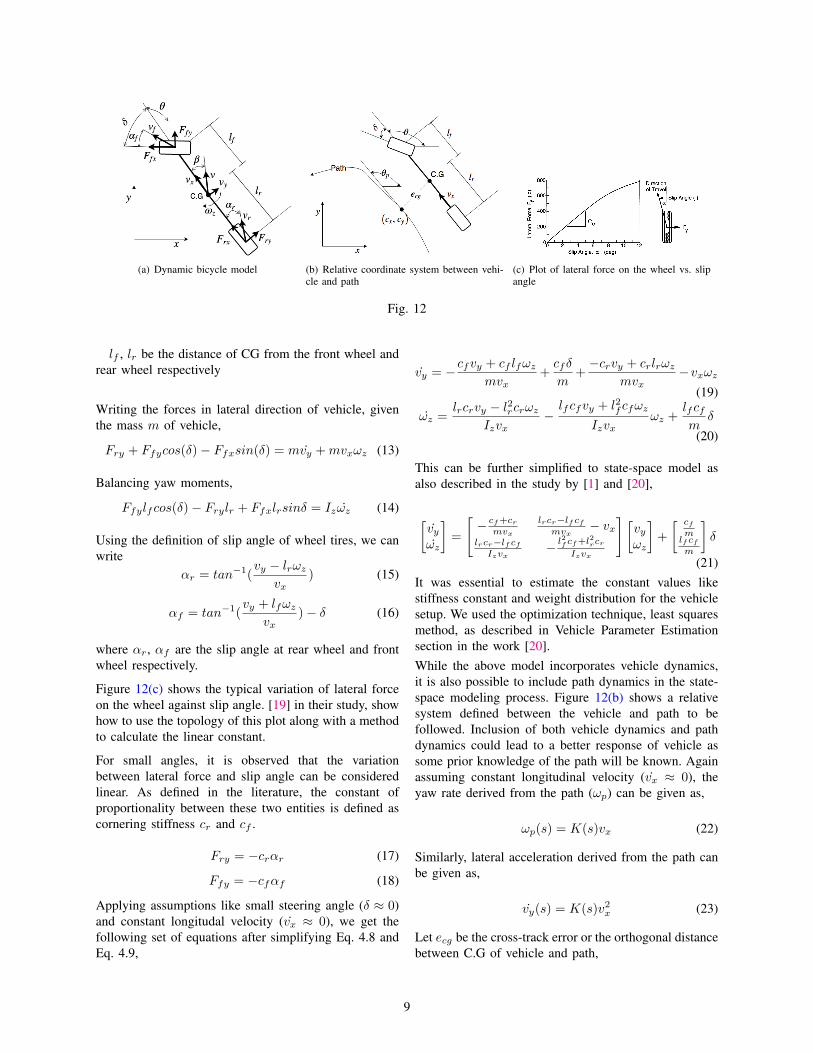
(a) Dynamic bicycle model (b) Relative coordinate system between vehi-cle and path

(c) Plot of lateral force on the wheel vs. slipangle

Fig. 12

lf , lr be the distance of CG from the front wheel andrear wheel respectively

Writing the forces in lateral direction of vehicle, giventhe mass m of vehicle,

Fry + Ffycos(δ)− Ffxsin(δ) = mvy +mvxωz (13)

Balancing yaw moments,

Ffylfcos(δ)− Frylr + Ffxlrsinδ = Izωz (14)

Using the definition of slip angle of wheel tires, we canwrite

αr = tan−1(vy − lrωz

vx) (15)

αf = tan−1(vy + lfωz

vx)− δ (16)

where αr, αf are the slip angle at rear wheel and frontwheel respectively.

Figure 12(c) shows the typical variation of lateral forceon the wheel against slip angle. [19] in their study, showhow to use the topology of this plot along with a methodto calculate the linear constant.

For small angles, it is observed that the variationbetween lateral force and slip angle can be consideredlinear. As defined in the literature, the constant ofproportionality between these two entities is defined ascornering stiffness cr and cf .

Fry = −crαr (17)

Ffy = −cfαf (18)

Applying assumptions like small steering angle (δ ≈ 0)and constant longitudal velocity (vx ≈ 0), we get thefollowing set of equations after simplifying Eq. 4.8 andEq. 4.9,

vy = −cfvy + cf lfωzmvx

+cfδ

m+−crvy + crlrωz

mvx−vxωz

(19)

ωz =lrcrvy − l2rcrωz

Izvx−lfcfvy + l2fcfωz

Izvxωz +

lfcfm

δ

(20)

This can be further simplified to state-space model asalso described in the study by [1] and [20],

[vyωz

]=

[− cf+crmvx

lrcr−lf cfmvx

− vxlrcr−lf cfIzvx

− l2f cf+l

2rcr

Izvx

] [vyωz

]+

[ cfmlf cfm

]δ

(21)It was essential to estimate the constant values likestiffness constant and weight distribution for the vehiclesetup. We used the optimization technique, least squaresmethod, as described in Vehicle Parameter Estimationsection in the work [20].While the above model incorporates vehicle dynamics,it is also possible to include path dynamics in the state-space modeling process. Figure 12(b) shows a relativesystem defined between the vehicle and path to befollowed. Inclusion of both vehicle dynamics and pathdynamics could lead to a better response of vehicle assome prior knowledge of the path will be known. Againassuming constant longitudinal velocity (vx ≈ 0), theyaw rate derived from the path (ωp) can be given as,

ωp(s) = K(s)vx (22)

Similarly, lateral acceleration derived from the path canbe given as,

vy(s) = K(s)v2x (23)

Let ecg be the cross-track error or the orthogonal distancebetween C.G of vehicle and path,

9

ecg = vy + vxsin(θe) (24)

where θe = θ − θp. After plugging (ecg , θp) into Eq.4.14 and Eq. 4.15, we get,

ecg =− cf + crmvx

ecg +cf + crm

θe +lrcr − lfcf

mvxθe

+lrcr − lfcf

mvxωp − vxωp +

cfmδ

(25)

θe =lrcr − lfcf

Izvxecg +

lfcf − lrcrIz

θe

−l2fcf + l2rcr

Izvx(θe + ωp) +

lfcfm

δ − ωp(26)

Using the above equations, we can form the state-spacemodel as,

ecgecgθeθe

=

0 1 0 0

0 − cf+crmvx

cf+crm

lrcr−lf cfmvx

0 0 0 1

0lrcr−lf cfIzvx

lf cf−lrcrIz

− l2f cf+l

2rcr

Izvx

ecgecgθeθe

+

0cfm0lf cfIz

δ +

0

lrcr−lf cfmvx

− vx0

− l2f cf+l

2rcr

Izvx

ωp(27)

B. Controller Synthesis

The presented controllers have been widely researchedin the past decade after the rise of autonomous vehicletechnology. Their implementation remains complicatedfor industrial and real-world utilization. Following sub-sections present them in a simplified manner for thepurpose of analysis and quick implementation.

(a) Geometry for pure pursuit (b) Geometry for stanley method

Fig. 13

1) Pure Pursuit: Pure Pursuit method is based on thegeometric model of the vehicle we defined previouslyin vehicle modeling section. This model is known to

approximate the tracking capability of the vehicle rea-sonably well at low speeds and up to moderate steeringangles. In this method, the goal point on the path to befollowed is determined by the look-ahead distance fromthe rear axle of the vehicle. Then, a circular arc thatconnects the rear axle of the vehicle and the goal pointis determined. Figure 13(a) shows the construction ofthese geometrical entities.Here,α be the angle between vehicle’s heading and look

ahead distance vectorR be the radius of curvature of the pathld be the look-ahead distance

Applying the sine law,

ldsin(2α)

=R

sin(π2 − α)

ld2sin(α)cos(α)

=R

cos(α)

ldsin(α)

= 2R

Curvature K can be defined as,

K =1

R=

2sin(α)

ld

We had already shown steering angle relation withturning radius as,

δ = tan−1(L

R) = tan−1(KL)

After combining the above equations, we get,

δ = tan−1

(2Leldl2d

)(28)

where eld is the lateral distance between the headingvector of the vehicle and goal point of the path.Implementing this controller involved tuning of the pa-rameter ld, i.e., look ahead distance. It was simple toconclude that for the overall stability of the vehicle ifthe longitudinal velocity of the vehicle is higher, thelook-ahead distance needs to be larger, and similarly, forlower longitudinal velocity the look-ahead distance willbe smaller. Thus, it was necessary to express look-aheaddistance as a function of velocity; for our purpose, wechose a linear function. So the final equation we usedfor tracking controller was,

δ = tan−1

(2Leldkv2x(t)

)(29)

where k is a tuning parameter.

10

Before implementing this control law on a simulatedvehicle or passenger car, we validated the model’s con-vergence using MATLAB. Figure 14(a) shows the quickreduction in cross-track error with time, thus allowingus to move ahead with this controller.

2) Stanley Method: This method comes from therobot system Stanley [3] that won the DARPA GrandChallenge. This method defines the steering control lawas a non-linear function of the cross-track error efa(taken from front axle here), that is, the distance betweenthe front axle of the vehicle and the nearest point on thepath. Intuitively, the law consists of two terms, one thathelps vehicle align to the heading of nearest path point(cx, cy) and the other that reduce the cross-track error.From Figure 13(b), we can write the control law as,

θe = θ − θp

Combining the two terms as per the definition,

δ(t) = θe(t) + tan−1

(kefavx(t)

)(30)

Comparing the above law with pure pursuit, there isan additional term, θe, that makes all the difference.Intuitively, this term adds more stability as it tries tocorrect the heading. Hence, it was expected that thismethod performs better than the pure pursuit for our setof experiments.

Convergence test for Stanley Controller shows decentresults as shown in 14(b)

3) PID Control: We defined the control law verysimilar to the previously derived PID velocity control.For this control, we assigned the process variable ascross-track error ecg , that is, the distance between theC.G of the vehicle and nearest path point. Similarly,the manipulated variable was assigned as the steeringangle input δ. Reference signal was considered constantof value 0, as for the path tracking capability we neededthe cross-track error to converge.Here,δ(t) be the steering angle input to vehicleecg be measured cross track errorr(t) be reference or set pointe(t) be the error signalKp, Ki Kd be the proportional, integral and derivative

constants respectively

Following equation was embedded into path trackingprogram,

δ(t) = Kpe(t) +Ki

∫e(t)dt+Kde(t) (31)

However, the above equation was converted to discreteform for actual use

δ(t) = Kpe(t) +Ki

t∑0

e(t) +Kde(t)− e(t−∆t)

∆t

(32)where ∆t is the sampling interval used for discretization.We tuned the PID constant values for low cross-trackerror and different desired specification than previouslydefined. They were,

• Steady-state error < 2%• Overshoot < 10%• settling time < 2 s

PID controller showed a very quick convergence time14(c) as compared to other methods as it can be tunedto be more aggressive while maintaining stability.

4) Linear Quadratic Regulator: LQR Control is oneof the most popular controller practiced in the fieldof optimal control theory. This controller is concernedwith operating a dynamic system (which in our case,the vehicle is) at minimum cost. The cost function isgenerally defined as a function of a property of thesystem that is targeted for attenuation. Similar to a PIDcontroller or pole placement method, the true essence ofapplying this method is to find an optimal gain matrix.Here, the optimality refers to the situation where thegains are not too high to saturate the signal input to theactuator or too low to be vulnerable to instability. Themethod involves no tuning parameters except the weightsassociated with minimizing the cost function.

We utilized the dynamic model of the vehicle aspreviously defined for implementation of LQR method.Eq. 4.25 can be written in the standard form of linearstate space equation as,

x = Ax+Bδ + Cωp (33)

where, A is the state transition matrix, B is the inputmatrix, and C is the residual matrix

A =

0 1 0 0

0 − cf+crmvx

cf+crm

lrcr−lf cfmvx

0 0 0 1

0lrcr−lf cfIzvx

lf cf−lrcrIz

− l2f cf+l

2rcr

Izvx

B =

0cfm0lf cfIz

C =

0

lrcr−lf cfmvx

− vx0

− l2f cf+l

2rcr

Izvx

All other variables hold the same terminology as definedin vehicle modeling section.And we defined the cost function as per the standard inliterature as,

11

J =

∫xTQsx+

∫uTQuu (34)

where Qs is the state cost matrix, and Qu is the inputcost matrix.

For linear systems like x = Ax + Bu it suffices todefine the feedback law as u = −Gx. However, weneeded a feedforward term in addition to the feedbackterm to cancel out the residual term in the Eq. 4.31. So,we defined the feedback law as,

δ = −Gx+ δff (35)

The study made by [1] includes a procedure to obtainthe appropriate expression for feedforward term forcanceling such residual terms. Using the same method,the final state-space model can be obtained as

x = (A−BG)x (36)

The above system is defined in continuous time domain.It was necessary to convert it to discrete time domainfor actual implementation. For example, a simple systemlike x = Ax + Bu in discrete form can be presentedas x[n + 1] = Adx + Bdu. Here, the continuoustime domain matrices (A and B) are discretized usingzero-order hold method to matrices Ad and Bd.

After following similar procedure as of continuous timedomain, we get the ultimate expression for embeddinginto our program,

x[n+ 1] = (Ad −BdG)x (37)

And the steering angle to update the vehicle position,

δ = −Gx+L

R(38)

where δff = LR is the calculated feedforward term.

The tuning parameters used for this controller were,

Qs =

q1 0 0 00 q2 0 00 0 q3 00 0 0 q4

where we defined q2 = q3 = q4 = 0, implying that thecross track error ecg is only being weighted towards thecontrol effort.and Qu was chosen as,

Qu = 1

to neglect the scaling between Qu and Qs.

The convergence test for LQR shows the importanceof the feed forward term as we observe a steady statecrosstrack error developing with the simple LQR con-troller without feed forward term.

5) Model Predictive Control: Model Predictive Con-trol (MPC) is another optimal control algorithm pro-ficient with multivariable systems where manipulatedvariables and outputs are subjected to specific constraintsin an optimized fashion. MPC follows a prolongedsuccess in process industries and therefore is rapidlyaccepted by the community in domains such as auto-motive, aerospace, city resources planning, and financialengineering. MPC can be considered to be a variantof LQR control strategy with additional features likeconstraints on manipulated variables (input to a plant)and optimization over N future steps instead of infinity.Recently, an increase has been observed in employingMPC for tasks of robot navigation [21], [22], [23]. Theworks which used MPC for steering control tasks inautonomous driving include [24], [25]. While the focusin [24] was on the inclusion of actuator dynamics andits effect in overtaking and lane change maneuvres, [25]focused on the task of following a reference trajectorysimilar to our case.

The name suggests the manner in which the controloutput is computed. At the present time t, the behavior ofthe system over the horizon N is considered. The modelpredicts the state over the horizon using control outputs.The cost function is thereafter minimized, satisfying thegiven constraints and control output for the next N stepsare calculated. Only the first computed predicted outputis used. At the time t+ 1, the computations are repeatedwith the horizon shifted by a one-time interval. Themathematical formulation can be given as,

U∗t (x(t)) := argmin

N−1∑k=0

q(xt+k, ut+k) (39)

subjected to,

xt = x(t) (40a)xt+k+1 = Axt+k +But+k (40b)xt+kεX (40c)ut+kεU (40d)Ut = {ut, ut+1, ..., ut+N−1} (40e)

The formulation uses prediction model 40b to estimatepossible state for N iterations. Equations 40c and 40ddefine the state and input constraints respectively. Forour purpose, the model is defined based on kinematicbicycle model as for other methods described in previoussubsections. This includes state of six parameters as x−yposition, θ orientation, vx longitudinal velocity, cte crosstrack error and ψ orientation error.

12

0 1 2 3 4 5

−0.2

−0.1

0

0.1

0.2

0.3

0.4

0.5

0.6

Time (in sec)

Cross track error (in m)

Pure Pursuit Convergence

Cross track error

Reference

(a) Pure Pursuit’s convergence of cross track error with time

0 2 4 6 8 10

−0.2

−0.1

0

0.1

0.2

0.3

0.4

0.5

0.6

Time (in sec)


Stanley Method Convergence

Cross track error

Reference

(b) Stanley Method’s convergence of cross track error with time

0 2 4 6 8 10

−0.2

−0.1

0

0.1

0.2

0.3

0.4

0.5

0.6

Time (in sec)


Simple PID Convergence

Cross track error

Reference

(c) PID controller’s convergence of cross track error with time

0 2 4 6 8 10

−0.2

−0.1

0

0.1

0.2

0.3

0.4

0.5

0.6

Time (in sec)


LQR Convergence

Cross Tracker Error

Reference

(d) LQR controller’s convergence of cross track error with time

Fig. 14

Model is defined as,

xt+1 = xt + vxcos(θt) ∗ dt

yt+1 = yt + vxsin(θt) ∗ dt

θt+1 = θt +vxLδt ∗ dt

vt+1 = vx

ctet+1 = f(xt)− yt + (vxsin(ψt) ∗ dt)

ψt+1 = θt − θp + (vxLδt ∗ dt)

While the model is non-linear, the control method isstill called linear MPC as the resulting cost functionis convex. The distinction between Non-Linear MPCand MPC does not reside in the fact that the model ofthe system is linear or non-linear, but the fact that theresulting cost function is convex or non-convex.

The cost function is defined such that it minimizes theerror in position, orientation along with penalizing moreuse and a sudden change of steering. The cost functionis calculated over the horizon of N time intervals. Allthe terms are weighted by their respective constants.Our work uses the IPOPT library for optimizing thecost function. It is an implementation of the primal-dual point-integral algorithm with a filter line-search

method for non-linear programming [26]. The furtherexplanation of the optimization process is beyond thescope of this work.

J =

N∑t=1

(wcte‖ctet‖2 + wψ‖ψt‖2) +

N−1∑t=1

wδ‖δt‖2

+

N∑t=2

‖δt − δt−1‖2

(41)

C. Simulation Results and Discussion

After the successful demonstration of control lawsconvergence in MATLAB, we went ahead with usingthe same laws for validating the results in a simulationenvironment. The results are in correspondence with theexperimental setup defined in Chapter 2 for simulation.

1) Pure Pursuit: Since the Pure pursuit method as-sumes a circular trajectory between the current positionand the target point at a specific look ahead distance, themethod was highly path specific. Initially, the look-aheaddistance was taken to be a product of the longitudinalvelocity and a constant. But when the results wereobserved, the parameter which was tuned for a specificvelocity didn’t work well for the other velocities. So after

13

(a) Straight course with velocity 10 kmph (b) Straight course with velocity 25 kmph (c) Straight course with velocity 35 kmph

(d) Circular course with velocity 10 kmph (e) Circular course with velocity 25 kmph (f) Circular course with velocity 35 kmph

(g) Lane change course with velocity 10 kmph (h) Lane change course with velocity 25 kmph (i) Lane Change course with velocity 35 kmph

(j) Sinusoidal course with velocity 10 kmph (k) Sinusoidal course with velocity 25 kmph (l) Sinusoidal course with velocity 35 kmph

Fig. 15: Pure Pursuit method’s plots for cross track error vs. distance travelled on straight course(a,b,c), circularcourse(d,e,f), lane change course(g,h,i) and sinusoidal course(j,k,l)

a lot of observations, it was concluded that the look-ahead distance should be,

Ld = k ∗ vx + d

The introduction of a fixed constant d led to a signif-

icant improvement in the results. To find the value of kand d, observations were made on the cross-track erroron various paths and velocities for a fixed parameterwhich was to be tuned. After finding this parameterfor different velocities, linear regression was appliedto get a relation between the look-ahead distance and

14





Fig. 16: Stanley method’s plots for cross track error vs. distance travelled on straight course(a,b,c), circularcourse(d,e,f), lane change course(g,h,i) and sinusoidal course(j,k,l)

longitudinal velocity.

The value of fixed constant d was found out bytrial-and-error, and the cross-track error was plotted fordifferent paths and velocities by varying the value of k.Intuitively, it was thought that with an increase in thevalue of look-ahead distance, the car would take longer

time to converge to the path, and hence the cross-trackerror would be more significant for the initial phase, anda steady-state error may be observed. By reducing thevalue of k, the tracking would become more aggressive.Reducing it beyond a particular value would lead tooscillations of the car about the path, and the car would

15

not be able to return back to the path.On a straight course as observed from Figure 15 (a)

(b) (c), there was a steady-state error of around 0.1m.Much change in results was not obtained by varyingthe value of k, and the error remained similar for allthe values. This was due to the fact that the methodcalculated an infinite radius curve between the currentposition and the point at a look-ahead distance. Theradius of curvature would remain infinity irrespectiveof the look-ahead distance due to the straight path andhence the controller would give an almost zero degreesteering angle. For a constant radius circular path asobserved from Figure 15 (d) (e) (f), the results werealmost similar for low velocities irrespective of the valueof k within a certain range. However, at higher velocities,a significant change was observed by varying the valuesof k. For high speeds, the higher values of k led to avery high steady-state error ( 0.5m) as compared to thatat lesser values of k where the error was around 0.2m.

The sinusoidal path contained all types of features,including varying radius of curvature. Thus, if the carwas correctly tuned for the sinusoidal path, it workedwith decent performance on all the other paths as well.Specific features were observed in the cross-track errorvs. distance along the path plot. The cross-track errorjumped to a higher value when the car approached themaxima and minima of the curve, whereas the errorwas less in magnitude during the remaining path. Theeffect of k was clearly visible for higher speeds as thecross-track error shooted to 0.5m at the maxima andminima of the curve. Since the pure pursuit controllerassumes a circular path between two points, it didn’tperform satisfactorily on a lane switching curve. Theresults were oscillatory, and errors were peaking up to0.5m for high speeds. By increasing the value of k,oscillations were attenuated but increasing it beyond aspecific value skipped the lane switching curve leadingto a significant amount of error.

Thus, overall, the pure-pursuit algorithm is a goodand computationally inexpensive geometrical method forpath tracking. It works satisfactorily for low speed andsimple curves but fails on higher speeds and complexcurves. Moreover, the tuning parameters were observedto be weakly path-dependent as well.

2) Stanley Method: The Stanley controller containstwo terms whose sum is used to calculate the steeringangle. The first term is used to make the steering wheelparallel to the tangent to the closest point on the path,whereas the second term is used to steer the car inwardstowards the path. The first term is the difference betweenthe heading of the vehicle and the heading of the path,whereas the second term is dependent on the cross-trackerror needs to be tuned. It was observed that the valueof the second term has some relation with velocity, but

its contribution is very less, so we have not made theterm velocity dependent for the simple reason of easytuning. Since the testing of the vehicle was done below35 kmph, the contribution has been ignored. Intuitively, itcan be thought that the more the velocity of the vehicle,the less should be the extra steering angle towards thepath; otherwise, it can lead to overshoot from the path.Thus, the velocity contribution if accounted for shouldbe added in the denominator of the second term. Figure16 shows the performance of this controller with tuningachieved within our capacity.

Tuning of the constant k was done for the sinusoidalpath as it contained varying radius of curvature. With theincrease in the value of k, the second term magnitudedecreased, and the vehicle was less responsive, and ittook more time to converge to the path. On decreasingthe value of k below a certain optimum number, theoscillations caused by it were visible. Thus, by trialand error method, the constant k was found out, andthe results were plotted for three different values of k.The cross-track error plot was similar to the sinusoidalwaveform. It reached maximum value corresponding tothe maxima of the sine wave. Moreover, the magnitudeof error was less than 0.5 m in all the cases. Thecontroller worked fairly for this path. For the circularpath of a constant radius, a steady-state error of around0.3-0.4 m was observed. To reduce this steady stateconstant error, the value of k was reduced, but it lead tooscillations, and thus, the error could not be minimizedfurther. Hence, the controller didn’t work well for sucha constant radius curve. On a straight path, the resultswere quite good with the error remaining zero in almostall cases. The minor oscillations were also not observed.The lane change path was tracked quite well below 35kmph. The effect of change in the value of k was clearlyvisible in this case. The maximum error for k = 5 wasmore significant than the maximum error for k = 3. Themaximum error remained below 0.5m.

Comparing the Stanley method with pure pursuit andPID, the controller worked comparatively better at highervelocities. Not much change was observed in the trackingresults with the change in velocity except for the lanechange case. Thus, this controller is better out of thethree for high-speed velocities. It was also found to bepath-dependent up to some extent.

3) PID Control: The PID steering method applieda simple PID feedback controller to the steering errorw.r.t the path. It was observed that the gains Ki andKd didn’t have a significant effect on a cross-track errorwhile the Kp gain had a noticeable impact. Hence, wefixed the gains Ki and Kd to a nominal value and onlyvaried Kp (manifested as k in legend) for further tuningobservations.

For the straight path, as observed in Figure 17 (a)

16





Fig. 17: PID method’s plots for cross track error vs. distance travelled on straight course(a,b,c), circular course(d,e,f),lane change course(g,h,i) and sinusoidal course(j,k,l)

(b) (c), the cross-track error kept oscillating within therange ±0.1 m at a lower speed. These oscillationsincreased with both an increase in speed and gain value.A low steady-state error was observed similar to the Purepursuit method with the help of gain Ki, but the vehicleunderwent small oscillations as it couldn’t steer small-

angle appropriately. For the circular path, the cross-trackerror was within a range of 0.3 m for tuned gains.Unusually, for a low value of Kp the cross-track errorboomed for all the speed ranges.

For the sinusoidal path, the error was within 0.25 mfor tuned constants. However, for a slightly lower Kp

17





Fig. 18: LQR controller’s plots for cross track error vs. distance travelled on straight course(a,b,c), circularcourse(d,e,f), lane change course(g,h,i) and sinusoidal course(j,k,l)

the error boomed to 0.8 m. As seen earlier, higher Kp

became unstable at higher speeds. This is again due tothe fact that the system overcompensated for a smallerror which leads to a resonating kind of error curve.For the lane change path, the performance profile wassimilar for all the 3 tried Kp values with only change in

the max error of this profile. However, for high speed, thetracking method failed to converge any of the gain Kp

values. This is due to the rapid change in the curvatureof the lane change path, which at high speed cannot betracked using a simple PID steering controller.

The results were highly parameter specific, and proper

18

tuning was required to achieve low average cross-trackerror and convergent tracking of the path. With a smallchange in parameters, the cross-track error varied by anoticeable margin. The tuning of parameters was alsoa trial-and-error process, and unlike other PID systemsnot intuitive for this purpose. Overall, we can label thePID steering method as a simple error reducing feedbackcontroller, which is only useful to use at low speeds forrelatively simple paths (no sharp changes in curvature).The tuning of gains is a tedious and non-intuitive processand often fails at different speeds.

4) Linear Quadratic Regulator: The LQR methodconsiders a linearized model for the vehicle and calcu-lates the optimal input for the system at any particularinstant. It guarantees asymptotic stability by finding thesolution to the Discrete Algebraic Ricatti Equation andusing the solution to find the optimal control action. Weweight the respective errors to decide the aggressivenessof the control action to minimize the respective error.From our synthesis described in the previous section,we keep parameter k = q1 as the only significant tun-ing parameter for simulation analysis. Figure 18 showsthe simulation results obtained on different courses byutilizing this controller. Other parameters that influencedthe controller were:

• The max iteration for the iterative solution ofDARE.

• The sampling time for the discrete-time model.• The tolerance for the iterative solution.While handling curves in the path tracking problem

the LQR controller had a decent performance in smoothpaths like on the circular course at normal velocitiesbut handling paths with quick changes in curvatureand higher velocities got difficult as at boundary pointsthe optimal control action shoots up beyond saturationand possibly due to non-linear dynamics dominatingat that time. That is, sudden changes in the path cur-vature brought about a perturbation that delayed theconvergence of the vehicle further. In addition to his,it was observed that the controller well handled constantcurvature paths at all velocities.

On paths with a change in concavity i.e., sinusoidalcourse, the controller didn’t track the path with minimalerror but at least presented robustness with varyingvelocity. With the incorporation of a velocity term withinthe state matrix of this controller, it performed robustlywith varying velocity for most of the courses tested.Overall, this controller, in its vanilla form performswell for low varying velocities on different courses andtherefore needs some modifications as discussed in theliterature for improving its performance on high speedand complex courses.

5) Model Predictive Controller: The Model Predic-tive Controller uses a predictive method where an inter-

nal model predicts the future states of the system andbased on the prediction it generates an optimal controlaction that minimizes a quadratic objective functionwhile satisfying certain constraints. This method helpsus to generate optimal control for the system withconstraints. For reference tracking, the method is verysuitable, considering the robustness and performance ofthe controller. We use an interior point optimizer libraryfor the optimization process in our case.

Parameters for MPC:• Objective function weights for respective error

terms.• Constraints for the control and state variables.• Predicted model for the system.• Prediction horizon.The basic strategy of tuning the MPC controller de-

pends on the optimizer used and the way it works. First,we need to set the constraints for the state and controlvariables, and then we need to change the weights forthe objective functions. Similar to the LQR controller,we can set the other weights to be zero initially and giveweight to just the cross-track error or randomly initializethe weights for other parameters. Once we know that theweights give an optimal control action, then we can workon fine-tuning. Figure 19 shows the performance of thiscontroller using the stated tuning strategy.

When running MPC on paths with abrupt changes inthe radius of curvature, we saw the benefit of having acontroller that predicts the future changes and optimizesthe control actions according to the changes. The con-troller outputs actions that can ensure continuous andsmooth tracking performance. However, on increasingthe prediction horizon, the performance is more affecteddue to more considerable computation time as well as amore significant effect of the future changes to currentcontrol action. An overall observation while using MPCcontroller was its robustness as the performance did notvary a lot with a change in paths as well as velocities.Being computationally heavy is the only demerit thatwas observed for the controller.

VI. EXPERIMENTS ON VEHICLE PLATFORM

After having implemented the path trackers on thesimulation world platform, we tested the same programson the dedicated passenger car used as a real-worldvehicle. Use of ROS came handy as it needed only afew changes to migrate the program from the simulationworld and to make them work for an actual passengercar.

A. Longitudinal Control

Similar to plant modeling for simulation world, wecollected the response data from the instrumented vehiclefor tuning the velocity control. Figure 20 shows the

19

(a) Lane change course with velocity 10 kmph (b) Lane change course with velocity 25 kmph (c) Lane Change course with velocity 35kmph

(d) Sinusoidal course with velocity 10 kmph (e) Sinusoidal course with velocity 25 kmph (f) Sinusoidal course with velocity 35 kmph

Fig. 19: Model predictive controller’s plots for cross track error vs. distance travelled on lane change course andsinusoidal course

response data on square wave throttle input for Mahindrae2o vehicle.

Fig. 20: Velocity response of vehicle to square wavethrottle input

The data obtained was very different than observedon the simulation platform. The acceleration and de-celeration of this vehicle have a different rate and alsonon-linear with the throttle. This made tuning the PIDcontroller manually much more difficult and estimatinggains using plant modeling was indeed a convenient wayout. MATLAB’s control toolbox gives the freedom toselect an appropriate rise time while estimating the gainvalue. We first considered a responsive controller by

setting the rise time to a low value. Figure 21(a) showsthe step response for vehicle’s velocity control using theestimated gain values with low rise time.

As observed, the response is significantly oscillating,which was not appropriate for path tracking purpose.With this aggressiveness, the rider comfort is also elim-inated, leave alone the steady-state error. Hence, weconsidered using a conservative rise time while tuningthe controller for better steady-state error and ridercomforts at the price of rise time. Figure 21(b) showsthe step response for vehicle’s velocity control using theestimated gain values with conservative rise time.

For the path tracking purpose on this vehicle platform,we restricted our experiments to vehicle velocity of 10kmph as per the availability of field-testing space. Wefirst tested the simple PID controller with the newlyestimated gain values for its performance on this veloc-ity. Figure 22(a) shows the performance of simple PIDcontroller for a trapezium reference profile.

As observed, the actual velocity did reach the max-imum velocity set point of 10 kmph using the steadilyincreasing reference input. This way of reaching the setpoint of 10 Kmph or higher velocity was found to besmoother and comfortable than directly giving 10 Kmphas a step reference. It is also noticed that the actualvelocity has two features, one being high-frequencyoscillations and the other being low-frequency oscil-

20

(a) Low rise time (b) Conservative rise time

Fig. 21: Unit Step Response

(a) Simple PID (b) Adaptive PID

Fig. 22: Performance of PID controller on Mahindra e2o

lations. The high-frequency oscillations are attributeddue to the presence of noise during actual velocitymeasurement and estimation. While the low-frequencyoscillation is attributed due to the bumpy surface on ourfield-testing space. This uneven surface perturbated theactual velocity during the experimentations and thereforecan be expected to be eliminated on road surfaces inan urban driving scenario. It should be noted that theseperturbations lowered the overall performance of thecontroller for tracking the velocity reference profile.

Further, the vehicle was tested with the presentedadaptive PID controller with the same velocity referenceprofile. Like discussed in simulation analysis of velocitycontrollers, we used the same gain values along with anominal gamma. Figure 22(b) shows the performanceof adaptive PID controller for the previous velocityreference profile. This controller performed better asit can be observed that the actual velocity profile iscloser to the reference profile. Also, the low-frequency

oscillations are seen to be dampened with the presence ofan adaptive nature. Overall, the adaptive PID controllerdid perform better; however, setting a nominal gammavalue doesn’t guarantee its performance under variousother conditions that remained untested.

B. Lateral ControlAfter having the velocity controller tuned, the vehicle

was tested with lateral control. A sample performance isshown using the Pure pursuit method with a maximumvehicle speed of 10 Kmph. Figure 23 shows the perfor-mance of pure pursuit path tracker on different coursesin terms of cross-track error.

As observed, even at such a low speed, the controllerfailed to reduce the cross-track error to zero. One ofthe primary reason is that the steering column fails todeliver the small input steering angle accurately, whichis required for path tracker to reduce the cross-trackerror to zero. The tire-ground interface provides enoughfriction that the execution of small steering angles by the

21

(a) Straight course (b) Lane change course (c) Circular course (d) Sinusoidal course

Fig. 23: Cross track error for pure pursuit tracker on different courses

(a) Straight course (b) Lane change course (c) Circular course (d) Sinusoidal course

Fig. 24: Cross track error for PID tracker on different courses

steering column fails that lets the error accumulate. Thiskind of observation was possible only after conductingexperiments on a real-world platform, which, on theother hand, was absent in the simulation world.

From experience of tuning the parameters for purepursuit on simulation, it was possible to relate the perfor-mance of the instrumented vehicle’s tracking capabilitywith the tuning parameter k. Figure 23 shows the tunedperformance that we were able to achieve. It is possibleto obtain better performance if more time can be spenton tuning the controller; however, for the scope ofthis work, it was only necessary to show the tuning(implementation) study.

Unlike the Pure pursuit tuning process, the PID con-troller was not observed to be very intuitive to be tuned.Figure 24 shows the performance of a tuned controllerthat we were able to achieve. This scenario is quitesimilar to the difficulties faced while tuning the PIDcontroller for simulation. Though in theory, it is knownthe importance of gains Kp, Ki & Kd as part of thetuning process; however, they were hardly found to bemimicked on our simulation and real-world data. More-over, its tuning was found to be much more involvingthan pure pursuit that was tuned with little effort. Hence,the PID steering law cannot be recommended for pathtracking purpose in general.

VII. CONCLUSIONS

This work presents some methods in the path trackingdomain for resolving the complex problem of accuratevehicle navigation. We first developed the experimental

setup required for simulation world performance eval-uation and later for real-world platform performanceevaluation. Development of a simulation world platformfor path tracking implementation eased the process ofdeveloping an individual tracker algorithm and allowedquick debugging of the complete workflow before it wasimplemented on the passenger car. Use of ROS as amiddleware framework for both simulation world vehicleand real-world vehicle ensured a smooth transition of thecodebase to our workstation for real-world experiments.Simulation world platform also allowed fast tuning ofcontrol algorithms, observations from which were usedto tune the same control algorithm on passenger car effi-ciently. The platform for the development of real-worldscenario was chosen as Mahindra e2o vehicle that isan all-electric CAN controlled vehicle. This vehicle wasequipped with various sensors like INS, wheel encoders,and also with a workstation as a controller’s computationunit. This instrumented passenger car platform allowedrobust experimental validation in different operating con-ditions, some of which cannot be accurately modeled ona simulation platform. Experiments were performed onthis vehicle with courses and velocity profile similar tothe ones mentioned in the simulation world subsection.This helped in observing and quantifying the deviationof a real-world physical system from a simulated worldone.

Since the path tracking problem comprises longitu-dinal control and lateral control, we developed themindependently. First, the longitudinal velocity controlwas developed as it is the pre-requisite to accurate

22

performance of lateral control. Using PID as a velocitycontroller was useful as it performed quite optimally onsimulation world data. Though the manually tuned con-troller wasn’t on par with industry grade performance,after having the plant modeled, a significant increasein performance was observed. Plant modeling was mosteffective using unit step response that was modified tosquare wave input for consensus calculation. Sinusoidalwave input also did model plant well; however, thesteering angle calculation using that model comprised ofhigh-frequency oscillations. This won’t be effective on areal-world platform as there exists a degree of latency be-tween calculation and performing the computed throttle.Hence, the plant modeled using sinusoidal wave inputwas ruled out. We verified the claim that adaptive PIDimproved performance over the simple PID method as itutilized learning gain values at every time step. AdaptivePID method also showed some resilience to changein vehicle mass that will be a frequently encounteredscenario in a real-world application.

The lateral control methods implemented in our workso far comprised of a geometric model and linearizeddynamic vehicle model. We rederived known methodslike Pure pursuit, Stanley, PID, LQR, and MPC forour use case and proved its convergence on MATLAB.Further, we used a computer simulator to demonstratethe working of our implementations of different pathtracking methods and also produced some plots forevaluating the performance for each of these methods.All of the controllers were tested on predetermined pathslike a straight line, circular course, lane shift course,and sinusoidal course. Rather than having them testedon a random driving course, they were validated againstspecific geometry of paths to provide insights to theirrelative advantages and disadvantages in an organizedmanner. A very detailed model can be cumbersome toobtain and use; thus, the tracking methods described inthis study made use of vehicle models that approximatevehicle motion. The simplifications, linearization, andsmall steering angle assumption of these models varied,which also led to the existence of a minimal cross-trackerror. From our simulation study, we concluded that upto medium level vehicle speed with an urban drivingscenario involving simpler paths, geometric methods ofpure pursuit and Stanley could be utilized. PID steeringmethod is not recommended in a real-world applica-tion specifically due to high sensitivity to gain values.LQR in its vanilla form gave descent performance onsimulation world data, but at times can go haywire ifthe calculations are not restricted to some limits. Thisproblem is solved in MPC, and therefore it performedwell under all scenarios even in its simplest form ofimplementation. This method is highly recommendedfor real-world application, the only difficulty being the

estimation of vehicle-specific parameters like the LQRmethod.

Implementation of path trackers on an instrumentedvehicle became easy after prototyping the controllersin the simulation world. Standardized development onROS made it possible to directly utilize the programsdeveloped for the simulation world for the instrumentedvehicle with some minor changes. Experience of tuningthe controller from a simulation vehicle also madeit easy to tune the vehicle platform. For longitudinalvelocity control, inaccuracies arose due to latencybetween the calculation of throttle value and its actualachievement. Moreover, the test arena available forexperimentation was an unleveled ground that usually isnot encountered in an urban driving scenario. Overall,the velocity controller was able to set the actual velocityto reference velocity as required for the appropriateperformance of the lateral control. Implementation ofpure pursuit and PID controller both were exactly thesame as used for gazebo vehicle. Tuning of pure pursuitwas as simple as in the simulation world, and a decentperformance was obtained that can be utilized for anurban driving scenario. Tuning of PID controller wastedious and time taking because of its unintuitive naturewhile steering towards path direction. This controller,therefore, is not recommended towards steering control,however, can be used for velocity control. Problems likereaction time of executing steering angle precisely andinability to execute small steering angle changes leadto deviation of real-world performance from simulationworld performance. Also, some of the unmodelleddynamics like steering column inertia and tire-roadinterface friction lead to performance degradation.These factors tend to affect more to the performanceof controllers at higher vehicle speed that was notexperimented within our study.The number and types of methods discussed in thisstudy yet are quite limited when compared to theexistence of massive literature on path trackers. Wewish to evaluate some more methods to bring acomparison based performance evaluation on a largescale. Also, the methods implemented in this studywere limited to vehicle velocity of 10 Kmph, 20 Kmph,and 35 Kmph. We wish to conduct experiments onmuch higher speeds like 45 Kmph + to get a significantamount of differences between these methods. Also, wewish to evaluate the path tracking capabilities on othercourses like an eight-figure shaped course, U-turn, andlong driving scenario for thorough analysis. Clearly,it was observed that MPC has a lot of scope to bethe ultimate path tracker algorithm for autonomousvehicles as per the simulation data. However, thebiggest challenge posed while implementing MPC forreal-time applications was the enormous computational

23

cost associated with optimization. For non-linearmodels, linearization of the model poses as anotheradditional challenge. Reducing these computationalcosts is an active topic in ongoing research. Availabilityof an accurate model is another major challenge. Theproposed solutions to this challenge include usingIterative or Learning MPC, which correctly learns thesystem model and/or modifies the cost function.

*Conflict of interest-none declared

REFERENCES

[1] J. M. Snider, et al., Automatic steering methods for autonomousautomobile path tracking, PhD Dissertation, Robotics Institute,Pittsburgh, PA, Tech. Rep. CMU-RITR-09-08.

[2] B. Paden, M. Cáp, S. Z. Yong, D. Yershov, E. Frazzoli, A surveyof motion planning and control techniques for self-driving urbanvehicles, IEEE Transactions on intelligent vehicles 1 (1) (2016)33–55.

[3] S. Thrun, M. Montemerlo, H. Dahlkamp, D. Stavens, A. Aron,J. Diebel, P. Fong, J. Gale, M. Halpenny, G. Hoffmann, et al.,Stanley: The robot that won the darpa grand challenge, Journalof field Robotics 23 (9) (2006) 661–692.

[4] R. C. Coulter, Implementation of the pure pursuit path trackingalgorithm, Tech. rep., Carnegie-Mellon UNIV Pittsburgh PARobotics INST (1992).

[5] A. Pandey, S. Jha, D. Chakravarty, Modeling and control ofan autonomous three wheeled mobile robot with front steer, in:2017 First IEEE International Conference on Robotic Computing(IRC), IEEE, 2017, pp. 136–142.

[6] H. Andersen, Z. J. Chong, Y. H. Eng, S. Pendleton, M. H. Ang,Geometric path tracking algorithm for autonomous driving inpedestrian environment, in: Advanced Intelligent Mechatronics(AIM), 2016 IEEE International Conference on, IEEE, 2016, pp.1669–1674.

[7] H. Ohta, N. Akai, E. Takeuchi, S. Kato, M. Edahiro, Pure pursuitrevisited: Field testing of autonomous vehicles in urban areas, in:Cyber-Physical Systems, Networks, and Applications (CPSNA),2016 IEEE 4th International Conference on, IEEE, 2016, pp. 7–12.

[8] N. H. Amer, K. Hudha, H. Zamzuri, V. R. Aparow, A. F. Z.Abidin, Z. A. Kadir, M. Murrad, Adaptive modified stanleycontroller with fuzzy supervisory system for trajectory trackingof an autonomous armoured vehicle, Robotics and AutonomousSystems 105 (2018) 94–111.

[9] A. Ollero, A. García-Cerezo, J. Martinez, Fuzzy supervisory pathtracking of mobile reports, Control Engineering Practice 2 (2)(1994) 313–319.

[10] A. De Luca, G. Oriolo, C. Samson, Feedback control of anonholonomic car-like robot, in: Robot motion planning andcontrol, Springer, 1998, pp. 171–253.

[11] N. Tavan, M. Tavan, R. Hosseini, An optimal integrated longi-tudinal and lateral dynamic controller development for vehiclepath tracking, Latin American Journal of Solids and Structures12 (6) (2015) 1006–1023.

[12] X. Heng, D. Cabecinhas, R. Cunha, C. Silvestre, X. Qingsong,A trajectory tracking lqr controller for a quadrotor: Design andexperimental evaluation, in: TENCON 2015-2015 IEEE Region10 Conference, IEEE, 2015, pp. 1–7.

[13] C. E. Garcia, D. M. Prett, M. Morari, Model predictive control:theory and practice—a survey, Automatica 25 (3) (1989) 335–348.

[14] A. Ollero, O. Amidi, Predictive path tracking of mobile robots.application to the cmu navlab, in: Proceedings of 5th Interna-tional Conference on Advanced Robotics, Robots in UnstructuredEnvironments, ICAR, Vol. 91, 1991, pp. 1081–1086.

[15] E. Kim, J. Kim, M. Sunwoo, Model predictive control strategyfor smooth path tracking of autonomous vehicles with steeringactuator dynamics, International Journal of Automotive Technol-ogy 15 (7) (2014) 1155–1164.

[16] P. Falcone, F. Borrelli, J. Asgari, H. E. Tseng, D. Hrovat,Predictive active steering control for autonomous vehicle systems,IEEE Transactions on control systems technology 15 (3) (2007)566–580.

[17] S. Sastry, M. Bodson, Adaptive control: stability, convergenceand robustness, Courier Corporation, 2011.

[18] L. Alonso, J. Perez-Oria, B. M. Al-Hadithi, A. Jimenez, Self-tuning pid controller for autonomous car tracking in urban traffic,in: System Theory, Control and Computing (ICSTCC), 2013 17thInternational Conference, IEEE, 2013, pp. 15–20.

[19] M. Doumiati, A. Victorino, A. Charara, D. Lechner, A methodto estimate the lateral tire force and the sideslip angle of a ve-hicle: Experimental validation, in: American Control Conference(ACC), 2010, IEEE, 2010, pp. 6936–6942.

[20] J. Ryu, State and parameter estimation for vehicle dynamicscontrol using gps., PhD Dissertation, Dynamics Design Lab,Stanford University, Stanford, CA 94305-2203.

[21] W. Schwarting, J. Alonso-Mora, L. Pauli, S. Karaman, D. Rus,Parallel autonomy in automated vehicles: Safe motion generationwith minimal intervention, in: 2017 IEEE International Con-ference on Robotics and Automation (ICRA), IEEE, 2017, pp.1928–1935.

[22] D. Kim, J. Kang, K. Yi, Control strategy for high-speed au-tonomous driving in structured road, in: 2011 14th InternationalIEEE Conference on Intelligent Transportation Systems (ITSC),IEEE, 2011, pp. 186–191.

[23] C. Katrakazas, M. Quddus, W.-H. Chen, L. Deka, Real-timemotion planning methods for autonomous on-road driving: State-of-the-art and future research directions, Transportation ResearchPart C: Emerging Technologies 60 (2015) 416–442.

[24] M. Babu, R. R. Theerthala, A. K. Singh, B. Gopalakrishnan,K. M. Kirshna, Model predictive control for autonomous drivingconsidering actuator dynamics, arXiv preprint arXiv:1803.03478.

[25] F. Borrelli, P. Falcone, T. Keviczky, J. Asgari, D. Hrovat, Mpc-based approach to active steering for autonomous vehicle sys-tems, International Journal of Vehicle Autonomous Systems 3 (2)(2005) 265–291.

[26] A. Wachter, L. T. Biegler, On the implementation of an interior-point filter line-search algorithm for large-scale nonlinear pro-gramming, Mathematical programming 106 (1) (2006) 25–57.

24

Documents

Design and Implementation of Path Trackers for Ackermann