Embed Size (px)
Citation preview

Design and Implementation of High Efficiency,
High Power Density Front-End Converter for
High Voltage Capacitor Charger
by
Yonghan Kang
Thesis submitted to the Faculty of the Virginia Polytechnic Institute and State University
in partial fulfillment of the requirements for the degree of
Master of Science in
Electrical Engineering
Dr. Fred C. Lee, Chairman
Dr. J. D. van Wyk
Dr. Fred Wang
April 15, 2005
Blacksburg, Virginia
Key Words: Capacitor charger, front-end converter, high power density, amorphous
core
Copyright 2005, Yonghan Kang

ii
Design and Implementation of High Efficiency, High
Power Density Front-End Converter for High Voltage
Capacitor Charger
Yonghan Kang
(ABSTRACT)
Pulse power system has been widely used for medical, industrial and military
applications. The operational principle of the pulse power system is that the energy
from the input source is stored in the capacitor bank or superconducting inductive
device through a dc-dc converter. Then, when a discharging signal exists, the stored
energy is released to the load through pulse forming network (PFN) generating high
peak power pulse up to gigawatts within several tens of or hundreds of
microseconds.
The pulse power system originally was developed for the defense application.
After the format of the voltage compression and voltage addition stages for the
short-pulse high power acceleration had been established, it has been evolved to be
common. Then, its application has been extended for food processing, medical
equipment sterilization and wastewater treatment since many present environmental
problems have been known in the early 70’s or even earlier. In addition, the pulse
power system is newly spotlighted due to the recent world events. The application
examples are to treat anthrax-contaminated mail and to make use of accelerators to
produce high power X-rays for security screening.

iii
Furthermore, the pulse power system has been applied for the tactical weapon
system such as electrothermal-chemical (ETC) gun, coilgun and active armor
system. Because the pulse power system applied for the tactical weapon system has
the potential to be integrated in the military vehicle, a compact lightweight pulse
power system is strongly required for the future weapon system.
In this thesis, a distributed power system (DPS) for the capacitor charger is
introduced for the application of the active armor system. A design methodology is
also presented for the front-end converter to achieve the high power density as well
as the high efficiency. Design parameters are identified, and their impact on the
design result is studied. Finally, the optimal operating point is determined based on
the loss comparison between different operating points.
In order to further improve the power density utilizing the unique operation
mode i.e. pulse power operation, transformer with an amorphous-based core is
designed and the result is compared with that using ferrite-based core. A 5 kW
prototype converter is built up and the experimentation is performed to verify the
design.

iv
In memory of
elder brother Seonghan

v
Acknowledgements
With my heartfelt gratitude, I would like to thank my advisor, Dr. Fred C. Lee
for his guidance, encouragement and continuous support throughout my studies
here. Although I fell behind his expectation, he was still ready to help and
encourage me. He is such a Great Mountain that nobody can easily climb or go
through. However, his severe challenging let me reflect myself and find my real
problems. It was priceless experience and lesson that only Dr. Lee’s student can
enjoy. I am sure that the rigorous research attitude I learned from him will benefit
every aspect in my life.
I am also very grateful to my committee members, Dr. J. D. van Wyk and Dr.
Fred Wang, for their valuable suggestions and help.
It has been a great pleasure to work with so many talented, creative, helpful
colleagues in the Center for Power Electronics Systems (CPES). Especially, I want
to express my special thanks to my mentors, Dr. Ming Xu and Dr. Wei Dong. They
have showed really good friendship with a full of encouragement and help. In turn,
it is natural that my thanks go to my colleagues in ARL project team for their
friendship, support, discussion and encouragement: Mr. Chuanyun Wang, Mr. Bing
Lu, Mr. Yang Qiu, Ms. Juanjuan Sun, Dr. Francisco Canales, Dr. Peter Barbosa, Dr.
Bo Yang, Mr. Wei Shen, Mr. Xigen Zhou, Mr. Honggang Sheng, Mr. Dianbo Fu,
Mr. Bryan Charboneau, Mr. Hongfang Wang, Dr. Xu Yang and Miss Ning Zhu.
I am also indebted to other colleagues. Their friendship has provided enjoyable
atmosphere: Dr. Jinghai Zhou, Ms. Li Ma, Dr. Yuancheng Ren, Mr. Yu Meng, Mr.
Doug Sterk, Mr. Ching-Shan Leu, Miss. Yan Jiang, Dr. Gary Yao, Mr. Yan Dong,
Mr. Arthur Ball, Ms. Qian Liu, Ms. Huiyu Zhu, Miss Jinghong Guo, Mr. Shuo
Wang, Mr. Sebastian Rosado, Dr. Lingyin Zhao and Dr. Rengang Chen.

vi
I would like to acknowledge CPES staffs, Ms. Trish Rose, Ms. Linda
Gallagher, Ms. Marianne Hawthorne, Mr. Robert Martin, Ms. Teresa Shaw, Ms.
Elizabeth Tranter, Ms. Anne Craig, Mr. Jamie Evans, Mr. Dan Huff, Ms. Michelle
Czamanske and Mr. David Fuller.
Many Korean fellows made my life in Blacksburg more enjoyable. I
especially thank Mr. Kisun Lee, Mr. Jounghu Park, Mr. Keun-Soo Ha, Mr.
Hongsun Lim, Mr. Unghee Lee, Mr. Kye-Hun Lee, Mr. Sung-Yeul Park, Mr. Hae-
Soo Kim and Mr. Dae-Woong Kim. Also, I appreciate Korean visiting scholars and
their family for their help and concern: Dr. Mango Kim, Dr. Seong-Jeub Jeon, Dr.
Juwon Baek.
Finally but not least, my sincere and heartfelt appreciation goes to my family
for their endless and unconditional love. My parents let me pursue my graduate
study in US although they were in the deep sorrow by losing their first son. Dad
and Mom! I can not forget your love forever. I also would like to thank my sister
Mijung Kang and brother-in-law Youngmook Choi for their help and
encouragement.
I have not been good husband and father after I came here with my wife and
first son. I have to spend most of my time in the Lab. After I got second son, the
situation was not chagned. I am really grateful to my wife, Misun Kim, and two
sons, Heechan and Youngchan, for their love and bright smiles that made me
encouraged and much happier than anything else.

Table of Contents
vii
Table of Contents
Acknowledgements ..........................................................................................................v
Table of Contents.......................................................................................................... vii
List of Figures .................................................................................................................ix
List of Tables................................................................................................................. xii
Chapter 1 : Introduction............................................................................................1
1.1 Background ......................................................................................................... 1
1.2 System Specifications and Challenges................................................................ 5
Chapter 2 : Literature Survey for Front-end Converter......................................10
2.1 Non-isolated Topologies ................................................................................... 10
2.2 Isolated Topologies ........................................................................................... 14
Chapter 3 : Power Stage Design of Active Clamp Full-bridge Boost Converter27
3.1 Design variables and their impact ..................................................................... 27
3.2 Selection of turns-ratio Tn ............................................................................... 30
3.3 Duty cycle constraints ....................................................................................... 32
3.4 Clamp capacitor voltage CV ............................................................................. 33
3.5 Volt-seconds of input inductor and transformer ............................................... 36
3.6 Zero voltage switching (ZVS) range................................................................. 38
3.7 Selection of design variables based on the loss estimation............................... 42
3.8 Design considerations of transformer ............................................................... 46
3.9 Transformer design using ferrite core ............................................................... 49
3.10 Experimentation using 1st prototype converter ................................................. 59

Table of Contents
viii
Chapter 4 : Transformer Design using Amorphous Core....................................62
4.1 Transformer size reduction by use of amorphous core ..................................... 62
Chapter 5 : Summary and Future Work ...............................................................68
Reference ........................................................................................................................71
Appendix ........................................................................................................................78
A. MatLab Code for Calculation of Conduction and Switching Losses..................... 78
Vita..................................................................................................................................84

List of Figures
ix
List of Figures
Fig. 1.1. Typical pulsed power system diagram................................................................1
Fig. 1.2. Conceptual diagram of coilgun system. ..............................................................3
Fig. 1.3. Distributed power system for capacitor charger. ................................................5
Fig. 1.4. Output current profile of front-end converter. ....................................................8
Fig. 2.1. Cascaded boost converter..................................................................................11
Fig. 2.2. The three-level boost converter.........................................................................12
Fig. 2.3. Cascaded three-level boost converter................................................................14
Fig. 2.4. (a) Isolated full-bridge boost converter and (b) its critical waveforms.............15
Fig. 2.5. Active clamp full-bridge boost converter. ........................................................17
Fig. 2.6. Full-bridge ZCS boost converter.......................................................................19
Fig. 2.7. Dual current-fed converter. ...............................................................................20
Fig. 2.8. LCC resonant converter. ...................................................................................22
Fig. 2.9. Loss comparison between two candidates. (a) Cascaded boost converter. (b)
Active clamp full-bridge boost converter. ................................................................24
Fig. 2.10. Component list to calculate the loss for (a) cascaded boost converter and (b)
active clamp full-bridge boost converter. .................................................................25
Fig. 3.1. (a) Active clamp full-bridge boost converter and (b) its critical waveforms....28
Fig. 3.2. Voltage conversion ratio over the function of duty cycle and turns-ratio.........32
Fig. 3.3. Operable duty cycle area over the function of series inductance and ...............34
Fig. 3.4 (a) Clamp capacitor voltage over the function of the series inductance and the
switching frequency and (b) comparison of on-resistance of MOSFET over the
function of the breakdown voltage. ..........................................................................35
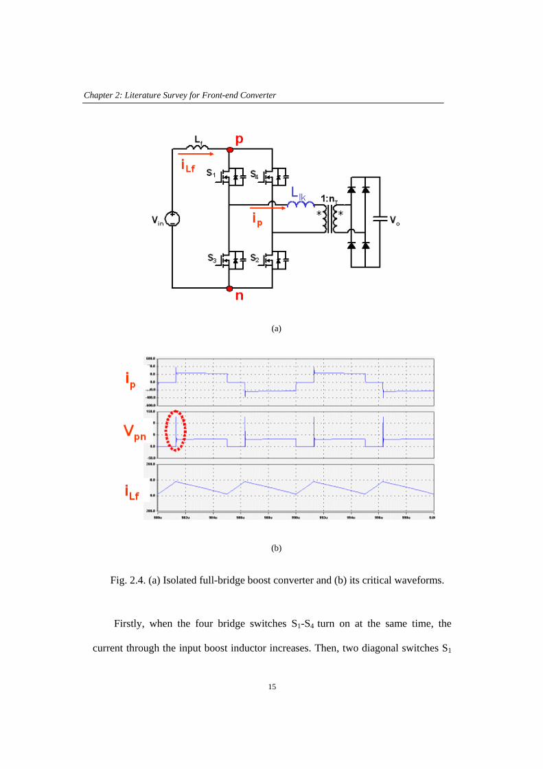
Fig. 3.5. Volt-second of input inductor over the function of the series inductance and
the switching frequency............................................................................................37
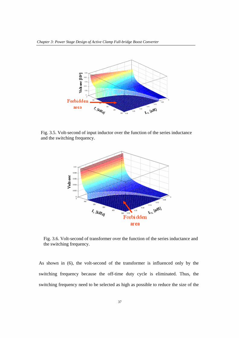
Fig. 3.6. Volt-second of transformer over the function of the series inductance and the
switching frequency..................................................................................................37

List of Figures
x
Fig. 3.7. (a) Switching transition between the turn-off of clamp switch and the turn-on
of all bridge switches and (b) the corresponding waveforms. ..................................39
Fig. 3.8. System structure and output current profile of the front-end converter............40
Fig. 3.9. ZVS range over the function of the series inductance and the switching
frequency. .................................................................................................................41
Fig. 3.10. Flow chart for the calculation of the primary-side loss...................................43
Fig. 3.11. Conduction loss of primary-side switches. .....................................................45
Fig. 3.12. Switching loss of primary-side switches.........................................................45
Fig. 3.13. Total loss of primary-side switches over the function of series inductance and
switching frequency..................................................................................................46
Fig. 3.14. Planar transformer structure. (a) Stand-alone structure. (b) Integrated
structure. The green rectangular box denotes PCB board. .......................................49
Fig. 3.15. Flow chart for transformer design...................................................................50
Fig. 3.16. E64/10/50 planar core from Ferroxcube and its dimensions. .........................50
Fig. 3.17. Two-winding example. (a) Flux distirbution. (b) Relationship between
magneto motive force F( )χ and magnetic field intensity H( )χ ...........................51
Fig. 3.18. Proximity effect of non-interleaved winding structure. ..................................53
Fig. 3.19. Three winding structures with different MMF profile. The red rectangular
box is primary winding, the blue rectangular box denotes secondary winding and
the green rectangular box represents the insulator of FR4. ......................................55
Fig. 3.20. 1-D thermal model for transformer. ................................................................57
Fig. 3.21. Transformer design results using ferrite core (a) when E64 core is used and
(b) when half-sized core is used. ..............................................................................58
Fig. 3.22 (a) 1st prototype converter and (b) its power stage parameters. .......................60
Fig. 3.23 (a) Experimental waveforms of the prototype converter where the upper most
waveform is the drain-to-source voltage of a bridge switch [50V/div], the
secondary waveform is the secondary current of the transformer [50A/div], the third
waveform is the output voltage [200V/div], and the lowest waveform is the output
current [5A/div]. Time [4µs/div]. (b) ZVS waveforms where the first line is the gate

List of Figures
xi
signal [20V/div] and the secondary line is the drain-to-source voltage of a bridge
switch. Time [0.4µs/div]...........................................................................................61
Fig. 3.24 Measured efficiency when input voltage is 24 V.............................................61
Fig. 4.1. Comparison of core loss density (a) when the peak flux density is 0.1 T and (b)
when the switching frequency is 100 kHz. The red line is for amorphous alloy J, the
pink line is for PowerLite, and the blue line is for High Flux Powder.....................64
Fig. 4.2. Comparison between ferrite 3F3 core and amorphous J alloy core. (a) Core
size comparison. (b) Loss and temperature comparison...........................................65
Fig. 4.3. 2nd prototype converter using amorphous core. ................................................66
Fig. 4.4. Experimental waveforms of 2nd prototype converter under the full load
condition (a) when the input voltage is 24 V and (b) when the input voltage is 30 V.
The pink line is the gate signal of one of four bridge switches [20V/div], the red
line is the drain-to-source voltage [50V/div], the green line is the current through
the secondary side of the transformer [20A/div] and the blue line is the output
voltage [500V/div]. Time [4µsec/div]. .....................................................................66

List of Tables
xii
List of Tables
Table 1.1 System specifications. .......................................................................................6
Table 2.1 Comparison between two candidates. .............................................................25
Table 3.1 MOSFETs used in the loss calculation and their characteristics....................43
Table 3.2. Maxwell 2D simulation results.......................................................................55
Table 4.1. Magnetic materials for transformer. ...............................................................63

Chapter 1: Introduction
1
Chapter 1 : Introduction
1.1 Background
Pulsed power is a suitable technology for driving electrical loads requiring
very large power pulses within short bursts. Figure 1.1 shows the typical pulsed
power system which consists of two main parts: One is the low power area and the
other is high power output stage. A battery and/or a generator work as primary
energy source, and its energy is transferred to the energy storage equipment by a
step-up dc-dc converter. The converter deals with relatively low average power
during the charging period. The energy from the energy source is stored in
capacitor bank or superconducting inductive device based on the applications. Then,
when a discharging signal exists, the stored energy is released to the load through
the pulse forming network, which determines the discharging period and power
pulse waveform, generating ultra high peak power up to gigawatts during very short
period in the range of micro- and millisecond.
Fig. 1.1. Typical pulsed power system diagram.

Chapter 1: Introduction
2
The pulsed power system has a wide spectrum of the applications in the
medical, industrial and military areas [A1-A23]. The simple example would be an
X-ray generator in the medical application where the X-ray is used for medical
diagnosis. In general, the X-ray generator is required to properly control the X-ray
penetration capability and beam quality such that the contrast, brightness and
resolution of X-ray images are good enough for medical diagnosis. In addition, the
volume and the weight are the important aspects in the applications such as X-ray
scanner, C-arm X-ray systems and portable X-ray machines [A1, A21].
Other examples can be found in the industrial applications: food irradiation,
radioactive and sewage waste treatment, surface hardening of steels, alloys and
semiconductors, surface cleaning, surface polishing, and so on [A4]. Among these
applications, many efforts have been exerted for the environmental applications
since many present environmental problems have been known in the early 70’s or
even earlier. After irradiation sources have been shown capable of destroying toxic
compounds now being identified as hazardous by-products of our industrial society,
many experiments have quantified the radiation necessary to kill bacteria harmful
to human being, such as e. coli and salmonella. Furthermore, the efforts are being
extended to material fabrication, chemical production, food pasteurization, medical
product sterilization, or as a treatment method for waste effluents that pollute the air,
ground soils, or ground water [A5-A7].

Chapter 1: Introduction
3
In addition to the previous medical and industrial applications, the pulsed
power system also has been applied to the military equipment. As a matter of fact,
the pulsed power system was developed for defense applications, and then the
format of the pulse compression and voltage addition stages for the short-pulse high
average power acceleration has been evolved to be common [A5]. Recently the
pulsed power system is being applied for new military applications such as electric
launchers, electrothermal-chemical (ETC) gun, coilgun, and active armor system.
Especially, ETC gun, coilgun and active armor system represent an advanced
weapon technology.
Figure 1.2 shows the conceptual capacitive-driven coilgun system. As shown
in Fig. 1.2, the conventional cannon can be used for the coilgun system with the
additional coil around it. In order to achieve the high speed in the muzzle, the
induction coilguns use magnetic coupling to drive current in the armature without
requiring direct electrical contact between barrel and projectile. Each of the barrel
coil shown in Fig. 1.2 is energized by its own capacitor bank. To create the moving
Fig. 1.2. Conceptual diagram of coilgun system.

Chapter 1: Introduction
4
magnetic wave in the barrel that is near-synchronous with the location of the
armature, a real-time detector locates the projectile and then the gun’s firing system
generates the trigger signal to close the switches of the capacitor banks of the
individual coils. The sequential discharge of current into successive coils ideally
creates a boundary condition of magnetic field for the armature that is near-constant,
allowing the armature to be magnetized with near-dc currents. These induced
currents penetrate more deeply into the conductor resulting in less localized heating
at the conductor surface than if higher frequency field variation occurred [A8-A11].
On the other hand, ETC gun also uses a conventional gun tube and combustion
chamber for the acceleration of a projectile. However, the system differs from
typical cannon weaponry in that it relies on the discharge of electrical energy stored
in the capacitor bank through an insulating capillary tube forming electrical plasma,
which is injected into the gun chamber to ignite and control the combustion of
propellant. Then, the discharge of electrical energy forms an arc that generates a hot,
high-pressure, low molecular-weight plasma source. The high temperature plasma
in the interior of the capillary causes ablation and vaporization of surrounding
insulation which is enveloped by hot gaseous material that sustains the original
plasma arc. The energetic plasma is then injected into a bed of chemical propellant
in the gun combustion chamber. The input plasma is utilized to first ignite the
propellant and then to drive as well as control the combustion process of the gun
[A12-A15].

Chapter 1: Introduction
5
Comparing to the pure electrical gun systems, coilgun and ETC gun
technology requires much less electric energy. Thus future pulsed power supply
systems for the applications have the potential to be integrated into a combat
vehicle. For mobile application such as the combat vehicle, the manufacture of
compact, light-weight and high efficient pulses power system is strongly required
due to the limited space of the military vehicle [A16, A17]
1.2 System Specifications and Challenges
Figure 1.3 shows a distributed power system (DPS) for a capacitor charger.
The capacitor charger is employed for an active armor system for future military
vehicle such as tank, armed vehicle and so on.
A battery powers the input of Fig. 1.3 and its operating voltage ranges from 24
V to 30 V. In addition, the front-end converter regulates the intermediate bus
voltage to 600 V whereas the load converter charges the output capacitor bank to 10
Fig. 1.3. Distributed power system for capacitor charger.

Chapter 1: Introduction
6
kV and then the output voltage is maintained by the trickle charging until a
discharging signal is applied. Five load converters charge the respective capacitor
bank and the capacitor banks can be connected in parallel to release the large
amount of the energy to the load at the same time or each capacitor bank would be
separately discharged according to the load requirement.
The capacitor charging system is assumed to be distributed around the
military vehicle: the front-end converter is placed at the inside of the vehicle such
that the front-end converter operates under 27℃ of the ambient temperature. The
temperature is maintained by a forced cooling method. On the other hand, the load
Table 1.1 System specifications.
Input voltage 24 V – 30 V
Intermediate bus voltage 600 V
Capacitor bank charging voltage 10 kV
Charging time 8 sec -10 sec
Total charging energy 20kJ
Power density > 50 W/in3 for each converter
System efficiency > 85 %

Chapter 1: Introduction
7
converter is equipped at the outside of the vehicle and operates under 49℃ of the
ambient temperature. The natural convective cooling method is applied for the load
converter. The detailed specifications are summarized in Table 1.1.
In order to clarify the operation and the design issues of the front-end
converter, firstly the operation of the load converter has to be explained. During the
charging period within 8 seconds to 10 seconds, the load converter operates under
the hybrid charging mode: Initially the load converter works under the constant
current charging mode to avoid the initial high current stress and this mode lasts
about 2 seconds. After that period, the load converter operates under the constant
power charging mode to reduce the charging power at the end of the charging
[A28]. Based on the operation of the load converter, the output current profile of
the front-end converter can be plotted as shown in Fig. 1.4. During two seconds, the
output current of the front-end converter increases because the charging power
increases. Then, until the charging ends, the output current of the front-end
converter remains constant due to the constant power operation of the load
converter. Hence it is clearly shown in Fig. 1.4 that the front-end converter has to
handle the full load current during the most period of the charging.
Except for the aforementioned, the design issues for the front-end converter
are summarized as follows:
1. In order to achieve 85 % of the system efficiency, the efficiency of each
converter should be higher than 92 %;

Chapter 1: Introduction
8
Fig. 1.4. Output current profile of front-end converter.
2. According to the specifications, the power density of the front-end converter
should be higher than 50 W/in3. The requirement of the power density is the
most stringent factor because the capacitor charging system will be
implemented in the inside of a military vehicle. The charging system can not
be voluminous due to the limitation of the available space in the military
vehicle.
3. High voltage conversion ratio ranging from 20 to 25 is also important factor
in the design stage because it would have influence on the selection of the
topology.
To cope with the challenges, Chapter 2 provides how to select the topology for
the specific application. The non-isolated converter and the isolated converter are
surveyed in the viewpoint of power density and efficiency, and then two converters
from each type converter are compared to select the best one.
Chapter 3 covers the design of the power stage of the selected topology. In this
chapter, the design parameters are identified and their impact on the operation

Chapter 1: Introduction
9
condition is studied. Based on the study, the optimal operating point is determined
in terms of the smallest total loss and the corresponding power stage parameters are
selected.
Also, Chapter 3 deals with the transformer design using the ferrite core. The
unique characteristic of the pulse power operation is utilized to shrink the size of
the transformer.
Chapter 4 is dedicated to the design of the transformer utilizing an amorphous-
based magnetic core to further reduce the size of the transformer. The comparison
between the ferrite-based transformer and the amorphous-based transformer is
given to emphasize the significant reduction of the transformer size.
Finally, Chapter 5 includes the summary and the future work.

Chapter 2: Literature Survey for Front-end Converter
10
Chapter 2 : Literature Survey for Front-end Converter
Because the system specifications do not require the isolation between the
input side and the output side of the front-end converter, the use of the transformer-
based converter would not be best solution unless there is study on the effect of the
isolated converter to the power density. Hence, several non-isolated and isolated
topologies are dealt with in the chapter. In order to select the best topology, the
advantages and the limitations of each converter are carefully taken into account.
Finally, two converters from non-isolated and isolated topologies are compared to
determine the best one.
2.1 Non-isolated Topologies
The single boost converter has been reported to be applicable in this
application [B1]. According to the system specifications, the converter has to step
up 24 V or 30 V of the input voltage to 600 V of the regulated intermediate bus
voltage where the DC voltage gain becomes 20 to 25. In order to provide such a
large DC gain, the conventional boost converter has to operate under quite large
duty cycle over 0.95. Also, considering the large input current the boost converter
needs to work in the continuous conduction mode (CCM) to reduce the current
stress of the main switch and the output rectifier. For the main switch and the
output rectifier, at least 1000 V rating MOSFET and diode should be used to block

Chapter 2: Literature Survey for Front-end Converter
11
600 V of the intermediate bus voltage. Under this operating condition, the boost
converter will experience sever reverse recovery problem in the output rectifier and
the main switch, which hurts the efficiency due to the increased switching loss. In
addition, the conduction loss of the main switch would be very large because the
high voltage rating device has normally large on-resistance. What is worst, the
output rectifier would not function properly due to the very short turn-on period and
in turn the output voltage would not increase to 600 V because of the conduction
loss and the large duty cycle [B2]. When no soft switching technique is applied to
the conventional boost converter, the switching frequency is generally limited to
around several kHz to reduce the switching loss. Accordingly, the size of the
passive components such as input inductor and output capacitor will be bulky,
causing power density to be reduced.
In order to avoid some aforementioned problems, Reference [B3] proposed a
cascaded boost converter as shown in Fig. 2.1, where the intermediate bus voltage
Fig. 2.1. Cascaded boost converter.

Chapter 2: Literature Survey for Front-end Converter
12
is established between two stages and two series connected converters share the
large voltage ratio. As shown in Fig. 2.1, this structure can solve the large duty
cycle problem. Also, the lower voltage rating MOSFET and diode can be placed in
the first stage converter resulting in the reduced conduction loss and reverse
recovery related loss. However, the reverse recovery problem still exists in the
secondary stage converter which prevents the switching frequency from being
increased. As a result, the passive component volume will be increased. In addition,
the total efficiency would be lower because the power processing occurs two times
in the cascaded converters. The control scheme also would be complex.
A non-isolated multilevel boost converter would be another option for the
front-end converter [B4-B8]. The three-level boost converter shown in Fig. 2.2 has
been successfully employed for power factor correction (PFC) circuit [B6-B8]. By
using a three-level structure, the converter can obtain some advantages over the
conventional boost converter. Firstly, the voltage stresses of the switches and the
rectifiers become half of the output voltage. Hence the low voltage rating MOSFET
Fig. 2.2. The three-level boost converter

Chapter 2: Literature Survey for Front-end Converter
13
and diode can be utilized to reduce the conduction loss. At the same time, the
reverse recovery related loss can be reduced when the low voltage rating diode is
applied for the rectifier. Furthermore, the current ripple frequency through the input
inductor becomes two times higher than the switching frequency, which enables the
size of the input inductor to be shrunk. Therefore, the power density and efficiency
of the converter will be improved although the number of the active components is
increased. However, the converter will still experience the large voltage conversion
ratio problem.
In order to solve the large voltage conversion ratio problem as well as to
maintain the advantages of the three-level boost converter, a cascaded three-level
boost converter can be introduced as shown in Fig. 2.3. With this cascaded structure,
the intermediate bus voltage VO1 is set to a voltage much lower than 600 V of the
output voltage VO. Hence the switches S1 and S2 as well as the output rectifier D1
and D2 in the first stage see a much lower voltage stress, which makes a low voltage
rating MOSFET and diode used for the switches and the rectifiers in the first stage.
The conduction loss and the reverse recovery related loss can be minimized. In
addition, the switches S3 and S4 and the rectifiers D3 and D4 in the secondary stage
experience a low current stress comparing to the single three-level boost converter,
which also would be helpful to reduce the conduction loss in the secondary side.
Furthermore, the size of the inductors L1 and L2 is much reduced since the current
ripple frequency through the inductors is two times higher than the switching
frequency, thus reducing the volt-second of the inductors.

Chapter 2: Literature Survey for Front-end Converter
14
Fig. 2.3. Cascaded three-level boost converter.
Taking the aforementioned advantages into account, the cascaded three-level
boost converter is selected for the candidate of the non-isolated converters. This
converter will be compared with another candidate of the isolated converters to
select the best topology for the front-end converter.
2.2 Isolated Topologies
This subsection covers the isolated converters for the front-end converter. The
isolated converter is basically derived from the boost converter although there are
converters which can not be classified into the boost converter.
Figure 2.4 shows the basic isolated bridge-type boost converter. In the
conventional boost converter, a transformer is introduced between the main switch
and the output rectifier. Then, the single switch is replaced with the full-bridge
configuration. Also, the secondary side of the transformer has the full-wave
rectifier configuration in place of the single output rectifier.
Chapter 2: Literature Survey for Front-end Converter
15
(a)
(b)
Fig. 2.4. (a) Isolated full-bridge boost converter and (b) its critical waveforms.
Firstly, when the four bridge switches S1-S4 turn on at the same time, the
current through the input boost inductor increases. Then, two diagonal switches S1

Chapter 2: Literature Survey for Front-end Converter
16
and S2 or S3 and S4 of the bridge switches are turned off and, in turn, a voltage is
exerted into the primary side of the transformer. The reflected voltage into the
secondary side of the transformer causes the two diagonal diodes D1 and D2 or D3
and D4, to turn on, and the secondary-side current of the transformer flows to the
load.
When the isolated boost converter is used, the large duty cycle operation can
be avoided by adjusting the turns-ratio of the transformer. Also, the voltage stress
of the bridge switches is reduced comparing with that of the non-isolated boost
converter. A low voltage rating MOSFET can be placed in the primary-side bridge
to reduce the conduction loss. In addition, the size of the input inductor can be
reduced because the current ripple frequency through the input inductor is two
times higher than the switching frequency, thus resulting in the reduction of volt-
second of the input inductor..
However, when the converter operates in the way explained in the above, the
bridge switches experience large switching since the switches turn on and turn off
under the hard switching condition. In addition, sine the current through the output
rectifier works in the continuous conduction mode (CCM), the output rectifier
would experience the excessive reverse recovery related loss due to the poor
reverse recovery characteristic of the high voltage rating diode. Furthermore, the
voltage VPN across the primary-side bridge sees the voltage spike as shown in Fig.
2.4 (b) due to the leakage inductance of the transformer when two diagonal

Chapter 2: Literature Survey for Front-end Converter
17
Fig. 2.5. Active clamp full-bridge boost converter.
switches turns off, which would offset the reduced voltage stress of the bridge
switches.
In order to solve the aforementioned problems, Reference [B9] proposed an
active clamp full-bridge boost converter as shown in Fig. 2.5. The active clamp
full-bridge boost converter basically has the same configuration as the isolated
boost converter in Fig. 2.4 except for the active clamp branch which features the
different operation comparing with the isolated boost converter.
Firstly, when all bridge switches S1-S4 turn on, the current through the input
inductor Lin increases. Then, two diagonal switches S1 and S2 or S3 and S4 turn off
and the clamp switch SC turns on with a small dead time. In this instant, the current
through the input inductor tries to go to the clamp switch instead of flowing through
the bridge switches since there is no initial current in the leakage inductance of the
transformer. As a result, the clamp capacitor CC is charged by the triangle current
determined by the current through the input inductor. During the turn-off period of

Chapter 2: Literature Survey for Front-end Converter
18
two diagonal switches, the current through the primary-side bridge switches starts
increasing from zero current to two times larger current than the average input
inductor current. The current is reflected into the secondary-side of the transformer
and flows to the load.
By this unique operation, the current through the secondary-side rectifier
works in the discontinuous conduction mode (DCM), resulting in the minimized
reverse recovery related loss. All the switches in the primary side can achieve the
zero voltage switching (ZVS) operation during the switching transition, which
reduces the switching loss in the primary side. In addition, the voltage VPN across
the primary-side bridge is clamped by the active clamp branch causing the voltage
stress to be minimized.
Figure 2.6 shows a full-bridge zero current switching (ZCS) boost converter
[B10] where each switch in the primary side has a serially connected diode to block
a reverse current through the body diode of the switch. Each switch in the primary
side can operate under the ZCS condition with constant frequency phase-shift
PWM control, resulting in the low switching loss. In addition, the current through
the output rectifier naturally commutates and thus the reverse recovery related loss
can be minimized.
The current through the resonant inductor Lr is clamped by the input inductor
current and the voltage across the resonant capacitor Cr is limited by the reflected

Chapter 2: Literature Survey for Front-end Converter
19
Fig. 2.6. Full-bridge ZCS boost converter.
output voltage. During the freewheeling period, the voltage across the resonant
capacitor changes its polarity by the resonance between Lr and Cr while the current
through the resonant inductor goes to the zero in a resonant fashion, enabling the
current through the output rectifier to naturally commutate. The leakage inductance
and the parasitic capacitance of the transformer can be incorporated into the
resonant inductor and the resonant capacitor.
However, the full-bridge ZCS boost converter experiences the large
conduction loss due to the serially connected diode in the primary side because the
forward voltage drop of the diode is much larger than the on-resistance of
MOSFET used as the bridge switch. Furthermore, the circulating energy would be
increased due to the large freewheeling period, which will increase the conduction
loss in the primary side.

Chapter 2: Literature Survey for Front-end Converter
20
Fig. 2.7. Dual current-fed converter.
Figure 2.7 shows the dual current-fed converter presented in [B11]. The input
inductor is separated into two branches and the switches S1 and S2 operate
complementally with a small dead time: when the switch S1 turns off, the switch S2
turns on, and vice versa. When the switch S1 turns on, the current through the
inductor L1 increases while the other current through the inductor L2 decreases. At
the same time, the current through the inductor L2 flows into the secondary side of
the transformer. As shown in Fig. 2.7, the inductors located in the primary side
have the half of the input current, and the primary side of the transformer also
carries the half of the input current. Thus, the copper losses of the inductor and the
transformer can be much reduced. As a result, the size of the inductor and the
transformer can be reduced due to the smaller current through them.
However, the switches in the primary side operate under the hard switching
condition, resulting in the large switching loss. Furthermore, the output rectifier

Chapter 2: Literature Survey for Front-end Converter
21
will experience the large reverse recovery related loss, which also increases the
switching loss.
By now, several PWM converters are surveyed for the front-end converter.
Another topology which can be applied for the front-end converter would be
resonant-type converter. The resonant converter has been widely employed for the
high voltage application because the converter can easily achieve the ZVS or the
ZCS and can absorb the parasitics presented by the high voltage transformer [B12-
B23].
The front-end converter has widely varying load condition: During the
discharging of the output capacitor bank, the whole system goes to the shut-down
mode. When there is another charging signal, the system start charging the
capacitor bank again. In this instant, the front-end converter sees an initial zero
output voltage. When the charging ends, the load converter in the system operates
under the trickling charging mode. Thus, the front-end converter will have a very
light load during the most period of the trickle charging.
Taking the operation of the front-end converter into account, the series
resonant converter is not good for the front-end converter because it is hard for the
series resonant converter to regulate the output voltage at the very light load
condition. In addition, the series resonant tank can not effectively absorb the
prasitics of the high voltage transformer. The parallel resonant converter is also not

Chapter 2: Literature Survey for Front-end Converter
22
Fig. 2.8. LCC resonant converter.
proper for the front-end converter because it is difficult for the parallel resonant
converter to regulate the output voltage under the short circuit condition although
the parallel resonant tank can absorb the parasitics of the high voltage transformer.
Another promising topology is the LCC or series-parallel resonant converter
shown in Fig. 2.8 [B20-B23]. The LCC resonant converter can fully absorb the
parasitics presented by the high voltage transformer. Also, the converter can work
well under the very light load condition as well as the short circuit condition.
Furthermore, the reverse recovery related loss can be minimized since the current
through the output rectifier commutates naturally.
However, the series capacitor CS in the primary side has to handle very large
current, requiring many capacitors connected in parallel to reduce the conduction
loss caused by its equivalent series resistance (ESR). This bulky capacitor would
deteriorate the power density. Also, the primary-side conduction loss will be larger

Chapter 2: Literature Survey for Front-end Converter
23
comparing with its PWM counterpart because the current through the primary-side
switches flows in the sinusoidal fashion resulting in the larger RMS current than
that of the square waveform current.
In summary, several PWM converters and resonant converters are considered
for the front-end converter. Their advantages and the shortcomings are addressed in
the loss and the power density viewpoints. Among the several converters, the
cascaded three-level boost converter in Fig. 2.3 and the active clamp full-bridge
boost converter in Fig. 2.5 are selected as the candidates for the front-end converter.
Figure 2.9 shows the loss comparison between two candidates. Firstly, the loss
of the cascaded three-level boost converter is calculated over the intermediate bus
voltage VO1. For the first stage, three different MOSFETs are used according to the
intermediate bus voltage. The voltage stress is set to 60 % of the rating voltage of
MOSFET. Hence, when the voltage stress is higher than 60 % of the rating voltage
of MOSFET, a higher rating voltage MOSFET is used to calculate the loss. Six
MOSFETs are placed in parallel for the first stage and the secondary stage switches
while one diode is used for each rectifier. After calculating the loss for each stage,
the total loss is obtained by combining each stage loss as shown in Fig. 2.9 (a).
The total loss of the active clamp full-bridge boost converter is also calculated
by the similar way. Primary-side loss and secondary-side loss are calculated over
the clamp voltage VC. Then, the total loss is combined together as shown in Fig. 2.9
(b). Six MOSFETs are connected in parallel for the bridge switch whereas four

Chapter 2: Literature Survey for Front-end Converter
24
(a)
(b)
Fig. 2.9. Loss comparison between two candidates. (a) Cascaded boost converter. (b) Active clamp full-bridge boost converter.

Chapter 2: Literature Survey for Front-end Converter
25
(a) (b)
Fig. 2.10. Component list to calculate the loss for (a) cascaded boost converter and (b) active clamp full-bridge boost converter.
Table 2.1 Comparison between two candidates.
Cascaded three-level boost converter
Active clamp full-bridge boost converter
Pre-charging circuit Yes Yes
Switching loss Large Small
Conduction loss Small Small
Natural commutation of output rectifier No Yes
Magnetic component size Small Small
MOSFETs are placed in parallel for the clamp switch. In addition, one diode is used
for each secondary-side rectifier. The components used for the calculation are listed
in Fig. 2.10.
As shown in Fig. 2.9, each converter shows the lowest loss when 75 V rating

Chapter 2: Literature Survey for Front-end Converter
26
MOSFET is used. In addition, the active clamp full-bridge boost converter has lower
total loss than that of the cascaded three-level boost converter although more
MOSFETs are used. Thus, the active clamp full-bridge boost converter is adopted for
the front-end converter. The comparison between two candidates is summarized in
Table 2.1.

Chapter 3: Power Stage Design of Active Clamp Full-bridge Boost Converter
27
Chapter 3 : Power Stage Design of Active Clamp Full-bridge Boost Converter
In the previous chapter, several PWM converters and resonant converters were
considered for the front-end converter and finally the active clamp full-bridge boost
converter (ACFBC) was selected as the best topology for the specific application.
This chapter deals with the design of the power stage of the converter. Firstly, the
design variables are identified and their impact on the operation condition is studied.
Then, the total loss is calculated over the function of the design variables and the
power stage parameters are selected for the lowest loss.
Also, the transformer design is presented using ferrite core. A difference to the
conventional transformer design is explained. A 5 kW prototype converter is
developed and the experimentation result is given to verify the design.
3.1 Design variables and their impact
According to the system specifications, the front-end converter must have
higher efficiency over 92 %. In addition, the power density of the front-end
converter should be higher than 50 W/in3. In order to satisfy these requirements, the
total loss should be as small as possible whereas the switching frequency has to be
selected as high as possible to reduce the size of the passive components. Figure 3.1
shows the active clamp full-bridge boost converter and its critical waveforms.

Chapter 3: Power Stage Design of Active Clamp Full-bridge Boost Converter
28
(a)
(b)
Fig. 3.1. (a) Active clamp full-bridge boost converter and (b) its critical waveforms.

Chapter 3: Power Stage Design of Active Clamp Full-bridge Boost Converter
29
When all the bridge switches are turned on, the input inductor current LfI
start increasing. During this period, the bridge switches in each leg share the input
inductor current. When two diagonal switches among the four bridge switches are
turned off, the clamp switch is turned on with a small dead time. In this instant, the
current LfI through the input inductor initially flows through the clamp switch and
charges the clamp capacitor in stead of going to the bridge switches because the
series inductance KL has no initial current at the instant and accordingly resists the
current through it to be abruptly changed. Thus, the current PI through the series
inductance increases from zero current to two times higher current than the average
input inductor current as shown in Fig. 3.1 (b).
In order to identify the design variables, firstly, the voltage conversion ratio of
the ACFBC is derived based on the operation of the converter. The voltage
conversion ratio is presented in (1).
O
in
2
K
2T
L
Ts
nL f
n
V 1 2MV (1 D ) 16
1 1R
(1 D )
= =−
+ +⎛ ⎞⎜ ⎟ −⎜ ⎟⎝ ⎠
(1)
From (1), it is shown that the voltage conversion ratio is influenced by the load
resistance LR as well as duty cycle D , which can be found in a converter operating
in DCM. Also, transformer turns-ratio Tn , series inductance KL , and switching

Chapter 3: Power Stage Design of Active Clamp Full-bridge Boost Converter
30
frequency Sf will have an effect on the voltage conversion ratio. Since the load
condition, input voltage range and output voltage are already defined by the
specification, the design variables are easily identified as turns-ratio, series
inductance and switching frequency. The design variables will determine the
magnitude of clamp voltage CV via the duty cycle and ZVS range as will be
explained late. In addition, the clamp voltage dictates the voltage stress of the
primary-side switches and will, in turn, influence on the conduction loss and the
switching loss. The ZVS range will also have effect on the switching loss.
Therefore, the design goal is to find the best combination of design variables
to achieve the high efficiency as well as the high switching frequency.
3.2 Selection of turns-ratio Tn
In this subsection, an extreme turns-ratio is assumed in order to clearly show
its effect on the voltage stress of the primary switches and the current stress of the
secondary rectifier.
When the transformer turns-ratio is assumed as 1 under the condition that the
input voltage is 24 V, the output voltage is 600 V and the efficiency is 92%, the
input inductor has to handle about 226 A of the average current. In this case, the
output rectifier has to carry two times higher peak current than the input inductor,
resulting in the large current stress in the secondary side. On the other hand, the
output voltage of 600 V is directly reflected into the primary side and accordingly

Chapter 3: Power Stage Design of Active Clamp Full-bridge Boost Converter
31
the voltage stress of the primary-side switches is also increased. Considering this
extreme example, the turns-ratio should be selected as large as possible to reduce
the voltage stress of the primary switches and the current stress of the secondary
diode.
Figure 3.2 illustrates the voltage conversion ratio over the function of the duty
cycle and the turns-ratio. The dotted line represents that the turns-ratio is 20; the
solid line denotes that the turns-ratio is 18; and the dash-dotted line is that the turns-
ratio is 16. Also, the red line is for no load condition whereas the blue line is for the
full load condition. The equation (1) can be simplified to (2) under no load
condition:
iT
O
n
V 1M @ RLV (1 D )
n= ≈ = ∞−
(2)
Under the no load condition, the voltage conversion ratio is only determined by the
turns-ratio and the duty cycle. Hence, when the turns-ratio is selected to a value, the
corresponding duty cycle is directly determined or vice versa.
As shown in Fig. 3.2, the minimum duty cycle is reduced as the turns-ratio is
increased. In general, the proper operation of PWM IC with the lower duty cycle
than 0.1 is not guaranteed. Also, when the zero of the duty cycle is allowed and
then the output voltage is higher than 600 V by somehow at no load condition, the
output voltage becomes out of the control. Thus, in order to secure the proper
operation of the converter the minimum duty cycle minD is selected as 0.1 and

Chapter 3: Power Stage Design of Active Clamp Full-bridge Boost Converter
32
Fig. 3.2. Voltage conversion ratio over the function of duty cycle and turns-ratio.
accordingly the turns-ratio is determined as Tn =18. Using the selected turns-ratio,
the duty cycle becomes 0.28 under the low line, no load condition.
Since the turns-ratio among the three design variables has been determined in
the subsection, the complexity of the design of the power stage is reduced. From
now on, the effects of the remaining two variables such as the series inductance KL
and the switching frequency Sf are considered on the duty cycle, clamp capacitor
voltage, volt-second of input inductor and transformer, and ZVS range.
3.3 Duty cycle constraints
From the voltage conversion ratio in (1), it can be easily realized that only the
series inductance and the switching frequency have influence on the duty cycle

Chapter 3: Power Stage Design of Active Clamp Full-bridge Boost Converter
33
after the turns-ratio is determined. In addition, the duty cycle has to be higher than
0.1 which is selected for the proper operation of the converter, and at the same time
the duty cycle should be lower than 1:
in sK To
o L i
T
n
V 4 V0.1 1
n n1
fV
LD
R V≤ = − + < (3)
Based on the constraint in (3), the duty cycle range for the proper operation of the
converter is illustrated in Fig. 3.3 where the converter can not operate in the
forbidden area because the duty cycle is higher than 1. Hence, the relationship
between the series inductance and the switching frequency is established: When the
switching frequency is selected as high as possible, the series inductance should be
as small as possible for the converter to work in the permitted area.
3.4 Clamp capacitor voltage CV
The clamp capacitor voltage is exerted to the input inductor when the two of
the bridge switches are turned off and the clamp switch CS is turned on. Hence the
clamp capacitor voltage is derived using the volt-second balance of the input
inductor as follows.
inC
K s
VV
1 D( L , f )=
− (4)
As shown in (4), the clamp capacitor voltage is also the function of series
inductance and switching frequency which have influence on the clamp voltage via

Chapter 3: Power Stage Design of Active Clamp Full-bridge Boost Converter
34
Fig. 3.3. Operable duty cycle area over the function of series inductance and
switching frequency.
the duty cycle. Therefore, the clamp capacitor voltage also has the operable area as
shown in Fig. 3.4 (a) where the duty cycle is located within the constraint of (3).
When a combination of the series inductance and the switching frequency is
selected close to the boundary between the operable area and the forbidden area, the
clamp capacitor voltage abruptly increases resulting in the higher voltage stress of
the primary-side switches as shown in Fig. 3.4 (a). In general, a high voltage-rating
MOSFET has the larger on-resistance comparing with the low voltage-rating
MOSFET. The comparison of the one-resistances between the different voltage
rating MOSFETs is given in Fig. 3.4 (b). As shown in Fig. 3.4 (b), the on-resistance
almost doubles as the voltage rating is increased. Furthermore, when 200 V rating
MOSFET is used, the on-resistance is four times higher than that of 150 V rating
MOSFET. Thus, the clamp capacitor voltage should be selected as low as possible
to reduce the conduction loss of the primary-side switches.

Chapter 3: Power Stage Design of Active Clamp Full-bridge Boost Converter
35
(a)
0.007050.0144
0.028
0.12
0
0.02
0.04
0.06
0.08
0.1
0.12
0.14
75 100 150 200BVDSS [V]
MOSFET
RDS(on)
[Ω]
0.007050.0144
0.028
0.12
0
0.02
0.04
0.06
0.08
0.1
0.12
0.14
75 100 150 200BVDSS [V]
MOSFET
RDS(on)
[Ω]
(b)
Fig. 3.4 (a) Clamp capacitor voltage over the function of the series inductance and the switching frequency and (b) comparison of on-resistance of MOSFET over the function of the breakdown voltage.

Chapter 3: Power Stage Design of Active Clamp Full-bridge Boost Converter
36
3.5 Volt-seconds of input inductor and transformer
Figures 3.5 and 3.6 shows the volt-seconds of the input inductor and the
transformer. During the turn-on period of all the bridge switches, the input voltage
is applied to the input inductor. Thus, the volt-second of the input inductor is
expressed as follows:
Sin K S in K S
S
T 1Volt sec V D( L , f ) V D( L , f )2 2 f
− = ⋅ = ⋅ (5)
As shown in (5), the volt-second of the input inductor is influenced by the series
inductance and the switching frequency via the duty cycle. In order to reduce the
size of the input inductor, the volt-second should be as small as possible. As shown
in Fig. 3.5, the switching frequency has to be increased and at the same time the
series inductance should be selected as small as possible to reduce the volt-second.
The volt-second also has the forbidden area where the duty cycle is out of the
constraints of (3).
On the other hand, the volt-second of the transformer can be determined
during the turn-off period of the two switches among all the bridge switches. At this
period, the clamp capacitor voltage works as the input voltage for the transformer.
Hence the volt-second of the transformer is represented as follows:
[ ] [ ] [ ]S in sC in
S
T V T 1Volt sec V 1 D 1 D V2 1 D 2 2 f
− = − = − =−
(6)
Chapter 3: Power Stage Design of Active Clamp Full-bridge Boost Converter
37
Fig. 3.5. Volt-second of input inductor over the function of the series inductance and the switching frequency.
Fig. 3.6. Volt-second of transformer over the function of the series inductance and the switching frequency.
As shown in (6), the volt-second of the transformer is influenced only by the
switching frequency because the off-time duty cycle is eliminated. Thus, the
switching frequency need to be selected as high as possible to reduce the size of the

Chapter 3: Power Stage Design of Active Clamp Full-bridge Boost Converter
38
transformer as shown in Fig. 3.6 since the series inductance does not have effect on
the volt-second of the transformer.
3.6 Zero voltage switching (ZVS) range
Figure 3.7 shows the switching transition period when the clamp switch turns off
and all the bridge switches turn on. In order to secure the ZVS operation of the two
bridge switches which was in the turn-off status during the previous period, the
energy stored in the series inductance should be large enough to discharge the output
capacitance 3C and 4C of the two bridge switches and the intrawinding capacitance
TrC of the transformer, and also to charge the output capacitance ScC of the clamp
switch. At the same time, some energy in the series inductance is to be transferred to
the load during this period. Hence, the minimum magnitude of the series inductance
to achieve ZVS operation can be derived considering the energy stored in the series
inductance and the energy to be needed to charge and discharge the total capacitance
as well as to be transferred to the load.
2 2 2Lf Lf eq O O
XK C
S
1 1 1( 2ID
L Vf
) ( I ) C V I2 2 2 2
⎡ ⎤− > +⎣ ⎦ (7)
where eqC denotes the equivalent capacitance of two output capacitances of the
bridge switches, the output capacitance of the clamp switch and the intrawinding
capacitance of the transformer. The ZVS operation should be achieved before the
current through the series inductance drops to half of its peak current as shown in

Chapter 3: Power Stage Design of Active Clamp Full-bridge Boost Converter
39
ip
Sc
S2
S1 S4
CcS3
LLK
Vin
1:nT
* *
Lf
Load
P
N
C1 C4
C2C3
Csc
CTr CoVo
+
-
+
-Vc
ic
iinLK
ip
Sc
S2
S1 S4
CcS3
LLK
Vin
1:nT
* *
Lf
Load
P
N
C1 C4
C2C3
Csc
CTr CoVo
+
-
+
-Vc
ic
iinLK
(a)
(b)
Fig. 3.7. (a) Switching transition between the turn-off of clamp switch and the turn-on of all bridge switches and (b) the corresponding waveforms.

Chapter 3: Power Stage Design of Active Clamp Full-bridge Boost Converter
40
Fig. 3.8. System structure and output current profile of the front-end converter.
Fig. 3.7 (b) because the current through the series inductance can not charge and
discharge the equivalent capacitance when the current is lower than the average
input current. The period when the ZVS operation should be finished is expressed
by XD and the switching frequency Sf in (7).
Figure 3.8 shows the system structure and the output current profile of the front-
end converter while the system is charging the output capacitive bank. As shown in
Fig. 3.8, the front-end converter has to handle the full load current during the most
charging period. Thus, the ZVS range is selected to the period when the output
current is higher than 80 % of the full load current. Using this selection and (7), the
ZVS range is plotted as shown in Fig. 3.9 over the function of the series inductance
and the switching frequency. For instance, if the switching frequency is selected to
500 kHz, the maximum series inductance has to be lower than 0.05 µH because the
clamp capacitor voltage is abruptly increased when the series inductance is chosen
higher than 0.05 µH. As a result, much more energy than the energy in the series

Chapter 3: Power Stage Design of Active Clamp Full-bridge Boost Converter
41
Fig. 3.9. ZVS range over the function of the series inductance and the switching frequency.
inductance is stored in the equivalent capacitance, which causes the converter to be
difficult to achieve the ZVS operation. However, the maximum series inductance is
reciprocally increased as shown in Fig. 3.9 as the switching frequency is reduced.
Taking into account the effect of the series inductance and the switching
frequency on the operation condition such as the duty cycle, the clamp capacitor
voltage, volt-seconds of the input inductor and the transformer, and the ZVS range,
it should be remarked that the switching frequency can not be selected too high due
to the limitation of ZVS range and also can not be too low because of the
constraints of efficiency and power density. In order to choose the proper switching
frequency to satisfy the requirements, a methodology should be built up: One way
is to calculate the loss over the function of the switching frequency and the series

Chapter 3: Power Stage Design of Active Clamp Full-bridge Boost Converter
42
inductance, and then the switching frequency and the series inductance to satisfy
the requirements are chosen.
3.7 Selection of design variables based on the loss estimation
In the previous subsections, the impact of the design variables such as the series
inductance and the switching frequency is studied on the duty cycle, the clamp
capacitor voltage, the volt-seconds of the input inductor and the transformer, and the
ZVS range. This subsection will cover the selection of the design variables. Firstly,
the conduction loss and the switching loss are estimated over the function of the
switching frequency and the series inductance, and then the specific values of the
design variables are determined with regard to the lowest loss.
Considering the circuit configuration of the secondary side in Fig. 3.1, the output
current flows through two diagonal output diodes during the turn-off period, and its
average current during the turn-off period is the same as the output current. Hence,
when CSD10120 from Cree, which is a 1.2 kV rating schottky SiC diode and its
maximum forward voltage drop is 3 V, is chosen for the output rectifier, the total loss
of four diodes is calculated as 50 W. Accordingly, the primary-side loss should be
much lower than 385 W to achieve the higher efficiency over 92%.
Figure 3.10 shows the flow chart to calculate the primary-side conduction loss
and the switching loss. The maximum series inductance is set to 0.3 µH and the
maximum switching frequency is 500 kHz. The turns-ratio of the transformer is fixed

Chapter 3: Power Stage Design of Active Clamp Full-bridge Boost Converter
43
Table 3.1 MOSFETs used in the loss calculation and their characteristics.
Clamp capacitor voltage
Vc < 52V 52V≤Vc<70V 70V≤Vc<100V 100V≤Vc<140V
Part name FDP047A08A0 FDP3632 FDP2532 FQP34N20
MOSFET BVDSS 75V 100V 150V 200V
RDS(on)@100℃ 7.05mΩ 14.4 mΩ 28 mΩ 120 mΩ
Qg 92nC 84nC 82nC 60nC
COSS 1nF 0.82nF 0.615nF 0.43nF
Fig. 3.10. Flow chart for the calculation of the primary-side loss.

Chapter 3: Power Stage Design of Active Clamp Full-bridge Boost Converter
44
to 18 which were determined based on the voltage stress of the primary-side switch
and the current stress of the secondary-side diode. The voltage stress of the
primary-side switches is kept to 50 % to 70 % of the rating voltage of MOSFET.
Hence, when the clamp capacitor voltage is increased over the predetermined
voltage stress, a higher rating voltage MOSFET is used to calculate the loss as
shown in Fig. 3.10. The MOSFETs used in the calculation and their characteristics
are summarized in Table 3.1. From Table 3.1, it is clearly seen that the on-
resistance is drastically shot up when a slightly higher rating voltage MOSFET is
used. Figures 3.11 and 3.12 show the conduction loss and the switching loss
calculated using the flow chart. It should be remarked that when the series
inductance is very small, the conduction loss of the primary-side switches is almost
similar to each other regardless of the switching frequency as shown in Fig. 3.11.
However, although the series inductance is very small, the switching loss is very
different over the switching frequency resulting in the much higher switching loss
than the conduction loss at the same series inductance. From Figs. 3.11 and 3.12, it
could be concluded that the switching frequency over 300 kHz can not be chosen
because the sum of the conduction loss and the switching loss is much larger than
385 W of the limitation.
Figure 3.13 shows the total loss of the primary-side switches. When the
switching frequency is 100 kHz and also the series inductance ranges over 0.035
µH to 0.065 µH, the total loss becomes lowest. Based on the loss estimation in Fig.
3.13, the switching frequency is determined to 100 kHz and the series inductance is

Chapter 3: Power Stage Design of Active Clamp Full-bridge Boost Converter
45
Fig. 3.11. Conduction loss of primary-side switches.
Fig. 3.12. Switching loss of primary-side switches.

Chapter 3: Power Stage Design of Active Clamp Full-bridge Boost Converter
46
Fig. 3.13. Total loss of primary-side switches over the function of series inductance and switching frequency.
chosen as 0.05 µH in order to allow the reasonable amount of loss to the magnetic
components such as the input inductor and the transformer.
3.8 Design considerations of transformer
Based on the specifications and the design results of the power stage, the
design inputs of the transformer are summarized as follows:
Power rating: 5 kW;
Switching frequency: 100 kHz;
Maximum input voltage: 30 V;

Chapter 3: Power Stage Design of Active Clamp Full-bridge Boost Converter
47
Maximum primary-side and secondary-side RMS currents: 239.6 A &
13.3A;
Turns-ratio: 1: 18;
Ambient temperature: 27 ℃;
∆TMAX (core surface to ambient): 53 ℃.
The maximum temperature of FR4 is recommended to around 105 ℃. In
addition, 100 is ℃ generally set for the smallest core loss although the core Curie
temperature is much higher than 100 ℃. Hence, the maximum core surface
temperature is selected to 80 ℃ taking the inner temperature of the core into
account. Before we start designing the transformer using the design inputs, several
design issues are considered to reduce the potential risk.
Firstly, for the ZVS operation of the converter as shown previously, some
amount of series inductance is necessary. Furthermore, the series inductance can be
comprised of only leakage inductance of the transformer or the combination of the
leakage inductance and an external inductor. If a large leakage inductance is
allowed in the transformer, it would cause EMI problem by the large uncoupled
flux. Also, the large leakage inductance will lead to the lower coupling efficiency
and in turn larger turns than the designed value should be placed to compensate the
lower coupling efficiency, which would increase the winding loss. Thus, the

Chapter 3: Power Stage Design of Active Clamp Full-bridge Boost Converter
48
leakage inductance is kept as small as possible and an external inductor is inserted
to provide the desired series inductance.
Secondly, planar transformer structure is considered due to the following
characteristics [C1, C2]:
1. Small leakage inductance can be achieved due to the good coupling
between the primary side and the secondary side;
2. Wider surface area can provide excellent thermal characteristics;
3. Low profile structure is easily achieved;
4. Owing to the good repeat ability of the properties, every assembly could
have the same characteristics.
Therefore, the transformer is constructed using the planar core, and the external
inductor whose inductance is 0.046 µH is implemented with MPP toroidal core
(MPP 55932) from Magnetics.
Thirdly, when the converter operates under the full load condition, the primary
RMS current of the transformer is 239.6 A. Hence the external inductor is placed
into the secondary side of the transformer to avoid the high current connection, thus
reducing the larger winding loss. In addition, the primary and the secondary
windings of the transformer are implemented utilizing the multilayer PCB board to
eliminate the large current junction point as shown in Fig. 3.14 (b).

Chapter 3: Power Stage Design of Active Clamp Full-bridge Boost Converter
49
(a)
(b)
Fig. 3.14. Planar transformer structure. (a) Stand-alone structure. (b) Integrated structure. The green rectangular box denotes PCB board.
3.9 Transformer design using ferrite core
Based on the previous considerations, the transformer is designed following
the flow chart shown in Fig. 3.15. In order to reduce the winding loss, 1 turn and 18
turns are chosen for the primary winding and the secondary winding, respectively.
The resultant core and its size are illustrated in Fig. 3.16, whose material is ferrite
3F3 from Ferroxcube. The cross-sectional area of the core is 5.19 cm2 and the
corresponding peak flux density peakB is 0.14 T.
Next, the leakage inductance and the proximity effect are considered to
determine the winding structure. Figure 3.17 (a) shows the typical flux distribution
generated within a two-winding transformer where the core has large
permeability oµ µ>> . The primary winding consists of eight turns of wire arranged

Chapter 3: Power Stage Design of Active Clamp Full-bridge Boost Converter
50
Fig. 3.15. Flow chart for transformer design.
Fig. 3.16. E64/10/50 planar core from Ferroxcube and its dimensions.
in two layers and each turn carries current i( t ) in the indicated direction. The
secondary winding is identical to the primary winding, except that the current
polarity is reversed. Within the transformer, a relatively large mutual flux is present,

Chapter 3: Power Stage Design of Active Clamp Full-bridge Boost Converter
51
(a)
(b)
Fig. 3.17. Two-winding example. (a) Flux distirbution. (b) Relationship between magneto motive force F( )χ and magnetic field intensity H( )χ [B2].

Chapter 3: Power Stage Design of Active Clamp Full-bridge Boost Converter
52
which magnetizes the core. In addition, leakage flux is present, which does not
completely link both windings. Owing to the symmetry of the winding geometry,
the leakage flux runs approximately vertically through the windings. Since the core
has large permeability, the magneto motive force (MMF) F( )χ induced in the
core by this flux is negligible. Hence the total MMF around the path is dominated
by the MMF across the core window as shown in Fig. 3.17 (b). Also, Ampere’s
Law indicates that the net current enclosed by the path is equal to the MMF across
the insulation layer of FR4 between two winding layers. Thus, the MMF across the
core window will be increased according to the number of the layer. Because the
magnetic field intensity H( )χ is proportional to the MMF F( )χ and the leakage
inductance is expressed by the function of the square of H( )χ as shown in (8) and
(9), the leakage inductance will increase abruptly if the windings of the primary
side and the secondary side are not sandwiched or interleaved [B2, C3-C7].
wF( ) H( ) lχ χ= ⋅ (8)
lkL ∝ 2H( )χ (9)
On the other hand, Fig. 3.18 shows the proximity effect between the stacked
winding layers. The primary winding consists of three series-connected turns of
copper foil with the thickness of h δ>> where δ is skin depth, and each turn
carries net current i( t ) . Under this situation, the high frequency current i( t ) flows

Chapter 3: Power Stage Design of Active Clamp Full-bridge Boost Converter
53
Fig. 3.18. Proximity effect of non-interleaved winding structure [B2].
on the right surface of primary layer 1. Then, the high frequency current induces a
copper loss in layer 1, which can be calculated as follows:
ac dchR Rδ
= (10)
21 acP I R= (11)
The proximity effect induces a current in the adjacent (left-side) surface of
primary layer 2 and the current tends to oppose the flux generated by the current of
layer 1. Since layers 1 and 2 are connected in series, they have to conduct the same

Chapter 3: Power Stage Design of Active Clamp Full-bridge Boost Converter
54
net current i( t ) . As a result, a current 2i( t )+ must flow on the right-side surface of
layer 2. Thus, the total copper loss in primary layer 2 is expressed as follows:
2 22 ac ac 1 1 1P I R ( 2I ) R P 4P 5P= + = + = . (12)
The copper loss in the second layer is five times larger than the copper loss in the first
layer. By the same phenomenon, the copper loss in the third layer becomes thirteen
times as large as the copper loss in the first layer [B2]. Hence, in order to minimize
the proximity effect it is necessary that the thickness should be close to the skin depth
δ , and the primary winding and the secondary winding are to be sandwiched or
interleaved as well [C3-C7].
Based on the above considerations, three winding structures for the
transformer are shown in Fig. 3.19. The total winding layers are 12 and the copper
thickness of each layer is 4 oz/ft2 which are smaller than the skin depth of 6.8 oz/ft2
at 100 kHz. The 6 layers among 12 layers are allotted for the primary winding and
the other 6 layers are used for the secondary winding, respectively. The 6 layers for
the primary winding are connected in parallel to reduce the winding loss and each
layer has one turn whereas the other 6 layers for the secondary winding are
connected in series and each layer consists of three turns to achieve 18 turns of the
secondary winding. The current density of the primary winding and the secondary
winding is 16 A/mm2.
As shown in Fig. 3. 19, Case I and Case II show the same peak magnitude of

Chapter 3: Power Stage Design of Active Clamp Full-bridge Boost Converter
55
pI6
P-S-P-S-P-S-P-S-P-S-P-S
Case I p2I6
MMF
pI6
P-S-P-S-P-S-P-S-P-S-P-S
Case I p2I6
MMF
Case II
P-S-S-P-P-S-S-P-P-S-S-P
pI6
p2I6
− pI6
MMF
Case II
P-S-S-P-P-S-S-P-P-S-S-P
pI6
p2I6
− pI6
MMF
Case III
P-P-S-S-P-P-S-S-P-P-S-S
pI6
p2I6
MMF
Case III
P-P-S-S-P-P-S-S-P-P-S-S
pI6
p2I6
MMF
Fig. 3.19. Three winding structures with different MMF profile. The red rectangular box is primary winding, the blue rectangular box denotes secondary winding and the green rectangular box represents the insulator of FR4.
Table 3.2. Maxwell 2D simulation results.
MMF while Case III has the largest MMF profile among the tree cases which will
result in the largest leakage inductance.
Table 3.2 shows the simulation results using the Maxwell 2-D simulator
(PEMag) from Ansoft. The simulated ac resistances are not much different between

Chapter 3: Power Stage Design of Active Clamp Full-bridge Boost Converter
56
three cases although Case I shows the smallest ac resistance. On the other hand,
Case III has the largest leakage inductance due to the largest MMF profile as
expected. Accordingly, Case I is determined as the winding structure for the
transformer.
After the core and the winding structure are determined, a thermal model is needed
to estimate the temperature rise of the transformer. Prior to developing the thermal
model, it should be kept in mind that the temperature would display a transient
characteristic, not steady state characteristic because of the pulse power operation
of the system. Thus, a thermal capacitance must be included in the thermal model
unlike the steady state thermal model. Figure 3.20 shows a 1-D thermal model
using an analogy to the electric circuit, which is applied for the core and the
winding, respectively. In Fig. 3.20, ambT is the ambient temperature, which is
27 ℃ by the specifications, and it is expressed by a voltage ambV in the electric
circuit. In addition, lossP denotes the core loss or the winding loss and is
represented by a current source. In the electric circuit of Fig. 3.20, the resistors
denote the thermal resistances of the core, the copper and the insulation material
(FR4). The thermal resistance is the function of the thermal conductivity (W/m℃)
of a material, the area (m2) and the length (m) through which the heat goes. On the
other hand, the capacitors represent the thermal capacitances of the core, the copper
and the insulation material and are the function of the volume (m3), the material
density (kg/m3) and the specific heat (J/kg℃) [C8-C17].

Chapter 3: Power Stage Design of Active Clamp Full-bridge Boost Converter
57
Fig. 3.20. 1-D thermal model for transformer.
Figure 3.21 illustrates the calculated core and winding losses and also the
simulated core and winding temperatures. Figure 3.21 (a) shows the result of the
first design where the core loss is much lower than the winding loss. Furthermore,
the core temperature and the winding temperature are lower than the maximum
allowable temperature. Thus, the length of the core is cut to the half as shown in Fig.
3. 21 (b) to reduce the size of the transformer, which results in two times as large as
the peak flux density. Accordingly, the core loss is increased over two times larger
than the core loss in Fig. 3.21 (a) due to the increased peak flux density. However,
the winding loss is a little bit reduced because the length of the winding is
shortened. Comparing two cases, the total transformer loss is not changed: the loss
of the first case is 121.3 W and the loss of the second case is 121.9 W. Although the
peak flux density is doubled and then reaches almost the saturation flux density
satB , the core temperature and the winding temperature are still lower than the

Chapter 3: Power Stage Design of Active Clamp Full-bridge Boost Converter
58
E 64
W
l
E 64
W
l
12.6W
108.7W
30℃
67.5℃
0
20
40
60
80
100
120
0.14
Core lossWinding lossCore temperatureWinding temperature
Bpeak [T]
12.6W
108.7W
30℃
67.5℃
0
20
40
60
80
100
120
0.14
Core lossWinding lossCore temperatureWinding temperature
Bpeak [T]
(a)
Half of E 64
Wl/2
Half of E 64
Wl/2
31.8W
90.1W
36.6℃
68.4℃
0
10
20
30
40
50
60
70
80
90
100
0.28
Core lossWinding lossCore temperatureWinding temperature
Bpeak [T]
31.8W
90.1W
36.6℃
68.4℃
0
10
20
30
40
50
60
70
80
90
100
0.28
Core lossWinding lossCore temperatureWinding temperature
Bpeak [T]
(b)
Fig. 3.21. Transformer design results using ferrite core (a) when E64 core is used and (b) when half-sized core is used.
maximum allowable temperature. Considering the temperature, there would be
possibility to further reduce the size of the transformer. However, taking the core
saturation into account, the size of the transformer could not be reduced any more
when the ferrite core is used.

Chapter 3: Power Stage Design of Active Clamp Full-bridge Boost Converter
59
3.10 Experimentation using 1st prototype converter
Figure 3.22 shows a 5 kW rating prototype converter and its power stage
parameters. The operating duty cycle ranges 0.1 to 0.41, and the maximum clamp
capacitor voltage is 41 V. Six MOSFETs are used in parallel for each bridge switch
whereas three MOSFETs are placed in parallel for the clamp switch. The achieved
power density is 45 W/in3.
Figure 3.23 shows the experimental waveforms under the condition that the
input voltage is 24 V and the output power is 5.1 kW. As shown in Fig. 3.23 (a), the
drain-to-source voltage of a bridge switch has a small voltage spike due to the
parasitics existing in the current path. The secondary-side current of the transformer
exhibits the DCM operation which causes the natural commutation of the current
through the output rectifier and helps the reverse recovery loss reduced. Figure 3.23
(b) shows the ZVS operation of a bridge switch. The efficiency is measured over
the different load condition when the input voltage is 24 V as shown in Fig. 3. 24.
The maximum efficiency is 91.9 % at 3.3 kW, and the full load efficiency is 91.3 %.

Chapter 3: Power Stage Design of Active Clamp Full-bridge Boost Converter
60
(a)
80% ~ full load
ZVS Range(@Vin=24V)
0.05μHLk
FDP047AN08A0(75V, 80A, 7.05mΩ)
MOSFET for primary switches
45 W / in3Power density of 1st prototype converter
1:18Turns Ratio (Np:Ns)
41VVc_max
0.1 ~ 0.41Duty Cycle
100kHzSwitching Frequency
80% ~ full load
ZVS Range(@Vin=24V)
0.05μHLk
FDP047AN08A0(75V, 80A, 7.05mΩ)
MOSFET for primary switches
45 W / in3Power density of 1st prototype converter
1:18Turns Ratio (Np:Ns)
41VVc_max
0.1 ~ 0.41Duty Cycle
100kHzSwitching Frequency
(b)
Fig. 3.22 (a) 1st prototype converter and (b) its power stage parameters.

Chapter 3: Power Stage Design of Active Clamp Full-bridge Boost Converter
61
(a) (b)
Fig. 3.23 (a) Experimental waveforms of the prototype converter where the upper most waveform is the drain-to-source voltage of a bridge switch [50V/div], the secondary waveform is the secondary current of the transformer [50A/div], the third waveform is the output voltage [200V/div], and the lowest waveform is the output current [5A/div]. Time [4µs/div]. (b) ZVS waveforms where the first line is the gate signal [20V/div] and the secondary line is the drain-to-source voltage of a bridge switch. Time [0.4µs/div].
Fig. 3.24 Measured efficiency when input voltage is 24 V.

Chapter 4: Transformer Design using Amorphous Core
62
Chapter 4 : Transformer Design using Amorphous Core
The previous chapter showed the selection of the power stage parameters, the
transformer design using the ferrite core, and the experimental results of the 1st
prototype converter. The achieved power density was 45 W/in3 which does not
satisfy the power density requirement. Thus, this chapter will focus on the
transformer design utilizing amorphous core to further enhance the power density.
In general, amorphous based core is not used to designing the high frequency
transformer due to its higher core loss density than that of the ferrite. However, this
chapter will show a new amorphous based core, which has much lower core loss
density comparing with other amorphous based cores, and its successful adoption to
the high frequency transformer.
4.1 Transformer size reduction by use of amorphous core
As aforementioned, the size of the transformer could not be reduced further
when the ferrite core is used because its saturation flux density is low and thus the
design result in Chapter 3 reached almost the limitation. Hence several different
magnetic materials are surveyed for the transformer as shown in Table 4.1. All
materials except for ferrite have higher saturation flux density over 1.4 T and also
their Curie temperatures are much higher than that of Ferrite. However, the initial
permeability is much lower than the initial permeability of ferrite except for

Chapter 4: Transformer Design using Amorphous Core
63
Table 4.1. Magnetic materials for transformer.
amorphous alloy J from Magnetics. In order to select the material suitable for
the transformer, the core loss density of each material is compared with that of
ferrite. Figure 4.1 shows the comparison of core loss density where the core loss
density of each material is normalized by the core loss density of ferrite. As shown
in Fig. 4. 1 (a) where the peak flux density is fixed to 0.1 T, the amorphous alloy J
shows the lowest core loss density among the three materials, and also its core loss
density is slightly higher than that of ferrite at the higher frequencies over 100 kHz.
In addition, when the switching frequency is set to 100 kHz, the core loss density of
the amorphous alloy J is lower than that of ferrite at the higher peak flux density
over 0.3 T as shown in Fig. 4.1 (b) which is more desirable to reduce the size of the
transformer by increasing the peak flux density. As a result, the amorphous alloy J
from Magnetics is employed for the transformer.

Chapter 4: Transformer Design using Amorphous Core
64
(a)
(b)
Fig. 4.1. Comparison of core loss density (a) when the peak flux density is 0.1 T and (b) when the switching frequency is 100 kHz. The red line is for amorphous alloy J, the pink line is for PowerLite, and the blue line is for High Flux Powder.
Figure 4.2 shows the comparison between the customized amorphous core and
the ferrite core. When the amorphous core is used, the peak flux density is
increased to 0.7 T. Accordingly, the length of the amorphous core is reduced to
20 % of E64 core although the height of the core is increased due to the

Chapter 4: Transformer Design using Amorphous Core
65
Ferrite (E64 core) Ferrite (Half size of E64 core) Amorphous alloy J
(a)
(b)
Fig. 4.2. Comparison between ferrite 3F3 core and amorphous J alloy core. (a) Core size comparison. (b) Loss and temperature comparison.
manufacturing difficulty of the amorphous core as shown in Fig. 4.2 (a). Also, the
volume of the amorphous core shrinks to 44 % of the volume of ferrite E64 core.
On the other hand, when the amorphous core is used, the core loss and the
winding loss are getting close to each other as the peak flux density increases as
shown in Fig. 4.2 (b), which will give the smallest total loss over the function of the
peak flux density. In addition, the temperatures of the core and the winding become

Chapter 4: Transformer Design using Amorphous Core
66
Fig. 4.3. 2nd prototype converter using amorphous core.
(a) (b)
Fig. 4.4. Experimental waveforms of 2nd prototype converter under the full load condition (a) when the input voltage is 24 V and (b) when the input voltage is 30 V. The pink line is the gate signal of one of four bridge switches [20V/div], the red line is the drain-to-source voltage [50V/div], the green line is the current through the secondary side of the transformer [20A/div] and the blue line is the output voltage [500V/div]. Time [4µsec/div].

Chapter 4: Transformer Design using Amorphous Core
67
close to each other as the losses converge. Comparing with the design result using
the ferrite core, the amorphous-based transformer shows a little bit higher total loss
than that of the ferrite-based transformer as shown in Fig. 4.2 (b). However, the
increase of the total loss is negligible. Figure 4.3 illustrates the 2nd prototype
converter utilizing the amorphous core. Its foot print is 6.72 × 5.29 in2, and the
power density is 49.7 W/in3 which satisfies the requirement. The core surface
temperature was measured under high line, full load condition, and it ranged
between 64 ℃ and 68 ℃ which are slightly higher than the simulation result.
Figure 4.4 shows the experimental waveforms of the 2nd prototype converter under
the full load condition. The output voltage was well regulated to 600 V. Also, the
drain-to-source voltage of the bridge switch and the current through the secondary
side of the transformer show that the converter works properly.

Chapter 5: Summary and Future Work
68
Chapter 5 : Summary and Future Work
Capacitor charging system has been widely used for the commercial, medical
and military applications. Recently, its technology has been taken attention again
due to the World events and the concerns about the environmental problems as well.
Furthermore, the capacitor charging system is being actively studied for the future
tactical weapon system. In this thesis, the specific application for the tactical armor
system was introduced, and its specifications were given. Also, the distributed
power system (DPS) for the capacitor charger was presented.
In order to satisfy the requirements to the front-end converter in the DPS,
several non-isolated and isolated converters were surveyed to find the suitable
topology. As a result, active clamp full-bridge boost converter was adopted for the
front-end converter because it has small conduction loss and switching loss. In
addition, the size of the magnetic components is small, and the converter operates
under ZVS condition.
Three design variables were identified for the design of the power stage of the
active clamp full-bridge boost converter and their impact on the design results were
investigated in term of conduction loss and switching loss. Finally, the optimal
values of the power stage parameters were determined for the smallest total loss.

Chapter 5: Summary and Future Work
69
The design result showed that the power density was a little bit smaller than
the requirement. Hence, in order to further improve the power density of the
converter, the thermal characteristic of the transformer was investigated under the
unique pulse power operation. As a result, it was found that the temperatures of the
core and the winding did not go to the steady state when the conventional design
step was applied for the transformer. Accordingly, the peak flux density was
increased to shrink the core size and the winding length. However, the size
reduction of the transformer was limited due to the lower saturation flux density of
the ferrite material.
Hence several different magnetic materials, which have the higher saturation
flux density, were surveyed, and then amorphous alloy J from Magnetics was
selected for the transformer. The transformer design result using the amorphous
core showed that the total transformer volume was shrunk to 44 % of the volume of
the ferrite-based transformer, keeping the total transformer loss to be almost same.
As a result, 49.7 W/in3 of the power density was achieved, which fully satisfies the
power density requirement. In addition, the converter operation was verified using
5 kW prototype converter.
The future work could include the integration of the series inductor and the
transformer. In the thesis, the series inductor and the transformer were implemented
using the different magnetic material and core. Although this approach met the
power density requirement, the size of the toroidal core for the series inductance

Chapter 5: Summary and Future Work
70
became comparable to that of the transformer when the size of the transformer was
reduced by using the amorphous core. Hence if the two magnetic components are
integrated together, the total size could be more shrunk. In addition, the total core
loss would be decreased when the two functions are implemented in one core.
Secondly, the small signal modeling of the active clamp full-bridge boost
converter can be also included for the future work. For this specific application,
there is no strict requirement to the fast transient response of the output voltage
because of the relatively slow charging profile ranging 5 seconds to 10 seconds.
However, some applications need very fast charging which has to be finished
within several micro seconds. Under this situation, the front-end converter will see
a very fast changing load and in turn need a high crossover frequency of loop gain
to avoid the larger overshoot or undershoot of the output voltage. For designing the
high crossover frequency of the loop gain, the small-signal modeling of the power
stage of the converter is prerequisite. After getting the small-signal model of the
power stage, feedback compensator can be designed for the voltage-mode control
or the current-mode control.

References
71
Reference
A. Pulse power and capacitor charging power systems, and their applications
[A1] M.A. Kempkes, J.A. Casey, M.P.J. Gaudreau, T.A. Hawkey and I.S. Roth, “Solid-state modulators for commercial pulsed power systems,” Proc. of Power Modulator Symposium, pp. 689-693, 2002.
[A2] M. Gundersen, J. Dickens and W. Nunnally, “Compact, portable pulsed power: physics and applications,” Proc. of Pulsed Power Conference, pp.9-12, 2003.
[A3] M. Buttram, “Some future directions for repetitive pulsed power,” IEEE Trans. on Plasma Science, vol. 30, no. 1, pp. 262-266, Feb. 2002.
[A4] M. Kristiansen, “Pulsed power applications,” Proc. of Pulsed Power Conference, pp. 6-10, 1993.
[A5] E. L. Neau, “Environmental and Industrial Applications of Pulsed Power Systems,” IEEE Trans. on Plasma Science. vol. 22, no. 1, pp. 2-10, Feb. 1994.
[A6] Xiangxiao Qiu, Laura Tuhela, and Q. Howard Zhang, “Application of Pulsed Power Technology in Non-Thermal Food Processing and System Optimization,” Proc. of Pulsed Power Conference, pp.85-90, 1997.
[A7] B. M. Penetrante, “Pollution Control Applications of Pulsed Power Technology,” Proc. of Pulsed Power Conference, pp.1-5, 1993.
[A8] Paul R. Berning, Charles R. Hummer, and Clinton E. Hollandsworth, “a Coilgun-Based Plate Launch System,” IEEE Trans. on Magnetics, vol. 35, no.1, pp. 136-141, Jan.1999.
[A9] Katsumi Masugata, “Hyper Velocity Acceleration by a Pulsed Coilgun using Traveling Magnetic Field,” IEEE Trans. on Magnetics, vol. 33, no. 6, pp.4434-4438, Nov. 1997.
[A10] Ronald J. Kaye, “Operational Requirements and Issues for Coilgun Electromagnetic Launchers,” IEEE Trans. on Magnetics, vol. 41, no. 1, pp.194-199, Jan. 2005.

References
72
[A11] Seong-Whan Kim, Hyun-Kyo Jung, and Song-Yop Hahn, “an Optimal Deisgn of Capacitor-Driven Coilgun,” IEEE Trans. on Magnetics, vol. 30, no. 2, pp.207-211, March 1994.
[A12] Yun-Sik Jin, et al. “Design and Performance of a 300 kJ Pulsed Power Module for ETC Application,” IEEE Trans. on Magnetics, vol. 37, no. 1, pp.165-168, Jan. 2001.
[A13] Gary L. Katulka, William F. Oberle, and Gloria P. Wren, “Pulsed-Power and High Energy Plasma Simulations for Application to Electrothermal-chemical Guns,” IEEE Trans. on Magnetics, vol. 33, no. 1, pp. 299-304, Jan. 1997.
[A14] Holger G. Wisken, Frank Podeyn, Thomas H. G. G. Weise, Jörg Dorn, and Dirk Westerholt, “Light Activated Semiconductors for ETC Pulsed Power Applications,“ IEEE Trans. on Magnetics, vol. 37, no. 1, pp.403-405, Jan. 2001.
[A15] W. Weck, J. Biebach, P. Ehrhart, A. Muller, and G. Reiner, “Power Supply System for ETC Type Launchers,” Proc. of Pulsed Power Conference, pp.369-372, 1999.
[A16] John A. Gaudet, et al. “Research Issues in Developing Compact Pulsed Power for High Peak Power Applications on Mobile Platforms,” Proc. of the IEEE, vol. 92, no. 7, pp.1145-1165, July 2004.
[A17] J. Biebach, P. Ehrhart, A. Müller, G. Reiner, and W. Weck, “Compact Modular Power Supplies for Superconducting Inductive Storage and for Capacitor Charging,” IEEE Trans. on Magnetics, Vol. 37, No. 1, pp. 353-357, Jan. 2001.
[A18] B.E. Strickland, M. Garbi, F. Cathell, S. Eckhouse and M. Nelms, “2 kJ/s, 25 kV high frequency capacitor charging power supply using MOSFET switches,” Proc. of Power Modulator Symposium, pp. 531-534, 1990.
[A19] R.M. Nelms and J.E. Schatz, “A capacitor charging power supply utilizing a Ward converter,” IEEE Trans. on Industrial Electronics, vol. 39, no. 5, pp. 421-428, Oct. 1992.
[A20] G. J. Rohwein, R. N. Lawson and M. C. Clark, “A compact 200kV pulse transformer system,” Proc. of Pulsed Power Conference, pp. 968-970, 1991.
[A21] Y.S. Jin, H.S. Lee, J.S. Kim, Y.B. Kim and G.H. Rim, “Compact 200kJ pulse power system with a simple crowbar circuit,” Proc. of Pulsed Power Conference, pp. 1239 – 1242, 2003.
[A22] M. Giesselmann and T. Heeren, “Rapid capacitor charger,” Proc. of Power Modulator Symposium, pp. 146-149, 2002.

References
73
[A23] M. Giesselmann and E. Kristiansen, “Compact Design of a 30 kV rapid capacitor charger,” Proc. of Pulsed Power Plasma Science, pp. 640-643, 2001.
[A24] H. Pollock, “High efficiency, high frequency power supplies for capacitor and battery charging” IEE Proc. of Power Electronics for Demanding Applications, pp. 901-910, 1999.
[A25] B.E.F. Cathell, S. Pronko, S. Eckhouse and N. Nelms, “8 kJ/s high frequency capacitor charging power supply using parallel inverters,” Proc. OF Pulsed Power Conference, pp. 245-248, 1995.
[A26] T. F. Wu, and J. C. Hung, “a PDM controlled Series Resonant Multi-level Converter Applied for X-ray Generators,” Proc. of IEEE Power Electronics Specialist Conference, pp. 1177-1182, 1999.
[A27] M. Souda, F. Endo, C. Yamazaki, K. Okamura, and K. Fukushima, “Development of High Power Capacitor Charging Power Supply For Pulsed Power Applications,” Proc. of Pulsed Power Conference, pp.1414-1416, 1999.
[A28] Yang Qui, Bing Lu, Bo Yang, Dianbo Fu, Lee, F. C., Canales, F. Gean, R., and Tipton W. C., “a High-frequency High-efficiency Three-level LCC Converter for High-voltage Charging Applications,” Proc. of IEEE Power Electronics Specialist Conference, pp.4100-4106, 2004.
B. Topologies for front-end dc-dc converter
[B1] P.K. Bhadani, “Capacitor-charging power supply for laser pulsers using a boost converter,” Rev. Sci. Instrum., pp. 605-607, 1989.
[B2] Robert W. Erickson, and Dragan Maksimovic, “Fundamentals of Power Electronics,” 2nd ed. Kluwer Academic Publishers, 2001.
[B3] L. Huber and M. M. Jovanovic, “A design approach for server power supplies for networking,” Proc. of IEEE Applied Power Electronics Conference, pp. 1163-1169, 2000.
[B4] B. Axelrod, Y. Berkovich and A. Ioinovici, “Transformerless DC-DC converters with a very high DC line-to-load voltage ratio,” Proc. of IEEE Int. Sym. on Circuits and Systems (ISCAS), pp. 435-438, 2003
[B5] O. Abutbul, A. Gherlitz, Y. Berkovich and A. Ioinovici, “Boost converter with high voltage gain using a switched capacitor circuit,” Proc. of ISCAS, pp. 296-299, 2003.

References
74
[B6] H. Wu and X. He, “Single phase three-level power factor correction circuit with passive lossless snubber,” IEEE Trans. on Power Electronics, vol.17, pp. 946-953, Nov. 2002.
[B7] B. Lin, Y. Hou and H. Chiang, “Implementation of a three-level rectifier for power factor correction,” IEEE Trans. on Power Electronics, vol.15, pp. 891-900, Sept. 2000.
[B8] M.T. Zhang, Y. Jiang, F.C. Lee and M.M. Jovanovic, “Single-phase three-level boost power factor correction converter,” Proc. of IEEE Applied Power Electronics Conference, pp. 434-439, 1995.
[B9] Kunrong Wang, Lizhi Zhu, Dayu Qu, hardus Odendaal, Jason Lai and Fred C. Lee, “Design, Implementation and Experimental Results of Bi-directional Full-bridge DC/DC Converter with Unified Soft-switching Scheme and Soft-starting Capability,” Proc. of IEEE Power Electronics Specialists Conference, pp.1058-1063, 2000.
[B10] Iannello, C. Luo, S, and batarseh, I., “Full-bridge ZCS PWM Converter for High-voltage High-power Applications,” Trans. on Aerospace and Electronic Systems, vol. 38, no. 2, pp.515-526, April 2002.
[B11] Wolfs, P. J., “a Current-sourced DC-DC Converter Derived via the Duality Principle from the Half-bridge Converter,” Trans. on Industrial Electronics, vol. 40, no. 1, pp.139-144, Feb. 1993.
[B12] R. Oruganti, J. Yang, and F.C. Lee, “Implementation of Optimal Trajectory Control of Series Resonant Converters,” Proc. of Power Electronics Specialist Conference, 1987.
[B13] A.K.S. Bhat, “Analysis and Design of a Modified Series Resonant Converter,” IEEE Trans. on Power Electronics, pp. 423-430, 1993.
[B14] J.T. Yang and F.C. Lee, “Computer Aided Design and Analysis of Series Resonant Converters,” Proc. IEEE IAS, 1987.
[B15] R. Oruganti, J. Yang, and F.C. Lee, “State Plane Analysis of Parallel Resonant Converters,” Proc. of Power Electronics Specialist Conference, 1985.
[B16] R. Liu, I. Batarseh, C.Q. Lee, “Comparison of Capacitively and Inductively Coupled Parallel Resonant Converters,” IEEE Trans. on Power Electronics, vol.8, pp. 445-454, 1993.

References
75
[B17] Y.G. Kang, A.K. Upadhyay, D. Stephens, “Analysis and Design of a Half Bridge Parallel Resonant Converter Operating Above Resonance,” Proc. IEEE IAS, pp. 827-836, 1998.
[B18] Robert L. Steigerwald, “A Comparison of Half Bridge Resonant Converter Topologies,” IEEE Trans. on Power Electronics, pp. 174-182, 1988.
[B19] R. Oruganti and F.C. Lee, “Resonant Power Processors, Part 2: Methods of Control,” IEEE Trans. on Industrial Application, 1985.
[B20] Shyh-Shin Liang, and Ying-Yu Tzou, “DSP Control of a Resonant Switching High-voltage Power Supply for X-ray Generators,” Proc. of Power Electronics and Drive Systems, pp.522-526, 2001.
[B21] M. Zaki, A. Bonsall, I. Batarseh, “Performance Characteristics for the Series Parallel Resonant Converter,” Proc. Southcon, pp.573-577, 1994.
[B22] A.K.S. Bhat, “Analysis, Optimization and Design of a Series Parallel Resonant Converter,” Proc. of Applied Power Electronics Conference, pp. 155-164, 1990.
[B23] A.K.S. Bhat, “Analysis and Design of a Series Parallel Resonant Converter with Capacitive Output Filter,” Proc. IEEE IAS, 1990, pp. 1308-1314.
[B24] B.J. Baliga, “Power semiconductor device figure of merit for high-frequency applications,” IEEE Electron Device Letters, pp. 455–457, 1989.
[B25] I. Kim; S. Matsumoto, T. Sakai and T. Yachi, “New power device figure of merit for high-frequency applications,” Proc. of Power Semiconductor Devices and ICs, pp. 309-314, 1995.
[B26] C. Rexer, Fairchild Semiconductor, “Advancements in power semiconductor solutions,” IEEE Applied Power Electronic Conference, Special Presentation Sessions, 2004.
C. Others
[C1] Ali I. Maswood and Lim Keng Song, “Design Aspects of Planar and Conventional SMPS Transformer: A Cost Benefit Analysis,” IEEE Trans. on Industrial Electronics, vol. 50, no. 3, pp.571-577, June 2003.
[C2] Application Note, “Design of Planar Power Transformer,” http://www.ferroxcube.com/
[C3] Ning Dai, “Modeling, Analysis and Design of High-frequency, High-density, Low-profile Transformers,” Dissertation, Virginia Tech, June, 1996.

References
76
[C4] R. Prieto, J. A. Cobos, O. Garcia, and J. Uceda, “Interleaving Techniques in Magnetic Components,” In Proceedings of the IEEE Applied Power Electronics Conference, 1997, pp.931-936.
[C5] Dirk van der Linde, Corlex A. M. Boon and J. Ben Klaassens, “Design of a High-Frequency Planar Power Transformer in Multilayer Technology,” IEEE Trans. on Industrial Electronics, Vol. 38, No. 2, April 1991, pp. 135-141.
[C6] Waseem A. Roshen, Robert L. Steigerwald, Richard J. Charles, William G. Earls, Gleen S. Claydon, and Chester F. Saj, “High-Frequency, High-Density MHz Magnetic Components for Low Profile Converters,” IEEE Trans. on Industry Applications, Vol. 3, No. 4, July/Aug. 1995, pp.869-878.
[C7] R. Prieto, J. A. Cobos, O. Garcia, P. Alou, and J. Uceda, “Taking Into Account All the Parasitic effects in the Design of Magnetic Components,” In Proceedings of the IEEE Applied Power Electronics Conference, 1998, pp.400-406.
[C8] Peter R. Wilson, J. Neil Ross and Andrew D. Brown, “Simulation of Magnetic Component Models in Electric Circuits Including Dynamic Thermal Effects,” IEEE Trans. on Power Electronics, Vol.17, No. 1, pp.55-65, Jan. 2002.
[C9] W. H. Tang, Q. H. Wu and Z. J. Richardson, “Equivalent heat circuit based power transformer thermal model,” IEE Proceedings of Electrical Power Application, Vol.149, No.2, pp.87-92, March 2002.
[C10] Joao C. S. Fagundes, Adalberto J. Batista and Philippe Viarouge, “Thermal Modeling of Pot Core Magnetic Components Used in High Frequency Static Converters,” IEEE Trans. on Magnetics, Vol.33, No.2, pp.1710-1713, March 1997.
[C11] Astrid Lewalter and Bernd Ackermann, “A Thermal Model for Planar Transformers,” In Proceedings of the IEEE Power Electronics and Drive Systems Conference, 2001, pp.669-673.
[C12] W.H. Tang, Q.H. Wu and Z.J. Richardson, “A Simplified Transformer Thermal Model Based on Thermal-Electric Analogy,” IEEE Trans. on Power Delivery, 2004, pp. 1112–1119.
[C13] G. Swift, T.S. Molinski and W. Lehn, “A fundamental approach to transformer thermal modeling. I. Theory and equivalent circuit,” IEEE Trans. on Power Delivery, 2001, pp. 171-175.

References
77
[C14] G. Swift and T.S. Molinski, “A fundamental approach to transformer thermal modeling. II. Field verification,” IEEE Trans. on Power Delivery, 2001, pp. 176-180.
[C15] P.E. Bagnoli, C. Casarosa, M. Ciampi, E. Dallago, “Thermal resistance analysis by induced transient (TRAIT) method for power electronic devices thermal characterization. I. Fundamentals and theory,” IEEE Trans. on Power Electronics, 1998, pp. 1208-1219.
[C16] L.-T Yeh and R.C. Chu, “Thermal Management of Microelectronic Equipment,” Textbook, New York: ASME Press, 2002.
[C17] F.P. Incropera and D.P. DeWitt, “Fundamentals of heat and mass transfer,” Textbook, New York: John Wiley & Sons, Inc., 2002.

Appendices
78
Appendix
A. MatLab Code for Calculation of Conduction and Switching Losses
The MatLab code shows one example to calculate the conduction loss and
switching loss generated in the primary-side switches when the switching frequency
is 100 kHz.
clear all; close all
%%%%%%%%%%%%%%%%%%%%%%%%%%%%%%%
% This is to calcualte the total loss of primary switches %
% including the clamp switch and the bridge switches %
% over series inductance and the switching frequency. %
%%%%%%%%%%%%%%%%%%%%%%%%%%%%%%%
u = 10^-9;
k = 1000;
Vo = 600;
Vin1 = 24;
nT=18;
RL=72;
IL1=Vo^2/(Vin1*RL);
fs1=100000;
Rdson_1=0.00705/6; % On-resistance of MOSFET
Rdson_2=0.0144/6;
Rdson_3=0.028/6;
Rdson_4=0.12/6;

Appendices
79
Rdson_11=0.00705/3;
Rdson_22=0.0144/3;
Rdson_33=0.028/3;
Rdson_44=0.12/3;
Qg1=9.2*10^-8; % Total gate charge of MOSFET
Qg2=8.4*10^-8;
Qg3=8.2*10^-8;
Qg4=6.0*10^-8;
Coss1=1.0*10^-9; % Output capacitance of MOSFET
Coss2=8.2*10^-10;
Coss3=6.15*10^-10;
Coss4=4.3*10^-10;
Vsp1=5.5; % Plateau voltage of each MOSFET
Vsp2=5.5;
Vsp3=4.5;
Vsp4=6.5;
Rdrive=1; % Gate drive resistor
Vdd=12; % Supply voltage for gate drive
%%%%%%%%%%%%%%%%%%%%%%%%%%%%%%%%%%%%%%%%%%%
%% The equivalent switching frequency of the clamp switch is 2fs because the clamp %
%% switch works two times within the switching period Ts while the equivalent %
%% switching frequency of the bridge switch is fs. %
%% In addition, it is assumed that three MOSFETs are used in parallel for the clamp %

Appendices
80
%% switch and six MOSFETs are placed in parallel for each bridge switch. %
%% Plus, each MOSFET in parallel for each switch shares the same amount of %
%% current through the switch. %
%%%%%%%%%%%%%%%%%%%%%%%%%%%%%%%%%%%%%%%%%%
i_max=200;
%%%%%%%%%%%%%%%%%%%%%%%%%%%%%%%%%%%%%%%%%%%
for i=1:i_max
x(i)=3*u + i*297*u/i_max; %%% ==> Lk
Dx11(i)=(4*nT*Vo*fs1*x(i))/(Vin1*RL); % Freewhleeing period of series inductance current
D11(i)=1-(nT*Vin1)/Vo+(4*nT*x(i)*fs1*Vo)/(Vin1*RL); % Duty cycle when Vin=24 ;
UD11(i)=IL1^2/3*Dx11(i)/2;
UD12(i)=(IL1/2)^2*(D11(i)-Dx11(i))/2;
UD13(i)=(2*IL1)^2/3*(1-D11(i))/2;
UD14(i)=(1/3)*((3*IL1/2)^2+(3*IL1/2)*(IL1/2)+(IL1/2)^2)*Dx11(i)/2;
UD15(i)=(IL1/2)^2*(D11(i)-Dx11(i))/2;
IrmsBr11(i)=sqrt(UD11(i)+UD12(i)+UD13(i)+UD14(i)+UD15(i));
IrmsT11(i)=4*IrmsBr11(i); % RMS current of four bridge switches
IrmsSC1(i)=sqrt((1/3)*4*IL1^2*(1-D11(i))); % RMS current of clamp switch
Vc11(i)=Vin1/(1-D11(i)); % clamp voltage
if (Vc11(i) > 0) & (Vc11(i) < 52)
Psw11B(i)=0.5*Vc11(i)*((2*IL1)/6)*fs1*Qg1*Rdrive/Vsp1+Qg1*Vdd*fs1+0.5*Coss1*Vc11(i)^2*fs1; %% Switching loss of one MOSFET for each bridge switch
Psw11C(i)=0.5*Vc11(i)*((IL1)/3)*(2*fs1)*Qg1*Rdrive/Vsp1+Qg1*Vdd*(2*fs1)+0.5*Coss1*Vc11(i)^2*(2*fs1); %% Switching loss of one MOSFET for clamp switch
Psw116B_4(i)=6*Psw11B(i)*4; %% Total switching loss of four bridge switches

Appendices
81
Psw113C(i)=3*Psw11C(i)*1; %% Total switching loss of the clamp switch
Psw11T(i)=Psw116B_4(i)+Psw113C(i); %% Total switching loss of the primary switches
PcondT11(i)=4*IrmsBr11(i)^2*Rdson_1+IrmsSC1(i)^2*Rdson_11; %% Total conduction
loss of the primary switches
Ptotal11(i)=Psw11T(i)+PcondT11(i); %% Total loss of the primary-side switches
elseif (Vc11(i) >= 52) & (Vc11(i) < 70)
Psw11B(i)=0.5*Vc11(i)*((2*IL1)/6)*fs1*Qg2*Rdrive/Vsp2+Qg2*Vdd*fs1+0.5*Coss2*Vc11(i)^2*fs1;%% Switching loss of one MOSFET for each bridge switch
Psw11C(i)=0.5*Vc11(i)*((IL1)/3)*(2*fs1)*Qg2*Rdrive/Vsp2+Qg2*Vdd*(2*fs1)+0.5*Coss2*Vc11(i)^2*(2*fs1); %% Switching loss of one MOSFET for clamp switch
Psw116B_4(i)=6*Psw11B(i)*4; %% Total switching loss of the bridge switches
Psw113C(i)=3*Psw11C(i)*1; %% Total switching loss of the clamp switch
Psw11T(i)=Psw116B_4(i)+Psw113C(i); %% Total switching loss of the primary switches
PcondT11(i)=4*IrmsBr11(i)^2*Rdson_2+IrmsSC1(i)^2*Rdson_22;
Ptotal11(i)=Psw11T(i)+PcondT11(i); %% Total loss of the primary-side switches
elseif (Vc11(i) >= 70) & (Vc11(i) < 100)
Psw11B(i)=0.5*Vc11(i)*((2*IL1)/6)*fs1*Qg3*Rdrive/Vsp3+Qg3*Vdd*fs1+0.5*Coss3*Vc11(i)^2*fs1; %% Switching loss of one MOSFET for each bridge switch
Psw11C(i)=0.5*Vc11(i)*((IL1)/3)*(2*fs1)*Qg3*Rdrive/Vsp3+Qg3*Vdd*(2*fs1)+0.5*Coss3*Vc11(i)^2*(2*fs1); %% Switching loss of one MOSFET for clamp switch
Psw116B_4(i)=6*Psw11B(i)*4; %% Total switching loss of the bridge switches
Psw113C(i)=3*Psw11C(i)*1; %% Total switching loss of the clamp switch
Psw11T(i)=Psw116B_4(i)+Psw113C(i); %% Total switching loss of the primary switches
PcondT11(i)=4*IrmsBr11(i)^2*Rdson_3+IrmsSC1(i)^2*Rdson_33;
Ptotal11(i)=Psw11T(i)+PcondT11(i); %% Total loss of the primary-side switches

Appendices
82
elseif ( Vc11(i) >= 100) & (Vc11(i) <= 140)
Psw11B(i)=0.5*Vc11(i)*((2*IL1)/6)*fs1*Qg4*Rdrive/Vsp4+Qg4*Vdd*fs1+0.5*Coss4*Vc11(i)^2*fs1; %% Switching loss of one MOSFET for each bridge switch
Psw11C(i)=0.5*Vc11(i)*((IL1)/3)*(2*fs1)*Qg4*Rdrive/Vsp4+Qg4*Vdd*(2*fs1)+0.5*Coss4*Vc11(i)^2*(2*fs1); %% Switching loss of one MOSFET for clamp switch
Psw116B_4(i)=6*Psw11B(i)*4; %% Total switching loss of the bridge switches
Psw113C(i)=3*Psw11C(i)*1; %% Total switching loss of the clamp switch
Psw11T(i)=Psw116B_4(i)+Psw113C(i); %% Total switching loss of the primary switches
PcondT11(i)=4*IrmsBr11(i)^2*Rdson_4+IrmsSC1(i)^2*Rdson_44;
Ptotal11(i)=Psw11T(i)+PcondT11(i); %% Total loss of the primary-side switches
else
Psw11B(i)=0.5*Vc11(i)*((2*IL1)/6)*fs1*Qg4*Rdrive/Vsp4+Qg4*Vdd*fs1+0.5*Coss4*Vc11(i)^2*fs1; %% Switching loss of one MOSFET for each bridge switch
Psw11C(i)=0.5*Vc11(i)*((IL1)/3)*(2*fs1)*Qg4*Rdrive/Vsp4+Qg4*Vdd*(2*fs1)+0.5*Coss4*Vc11(i)^2*(2*fs1); %% Switching loss of one MOSFET for clamp switch
Psw116B_4(i)=6*Psw11B(i)*4; %% Total switching loss of the bridge switches
Psw113C(i)=3*Psw11C(i)*1; %% Total switching loss of the clamp switch
Psw11T(i)=Psw116B_4(i)+Psw113C(i); %% Total switching loss of the primary switches
PcondT11(i)=4*IrmsBr11(i)^2*Rdson_4+IrmsSC1(i)^2*Rdson_44;
Ptotal11(i)=Psw11T(i)+PcondT11(i); %% Total loss of the primary-side switches
end
if (Vc11(i) > 140)
break;
end
if (D11(i) >= 1)
break;

Appendices
83
end
end
%%%%%%%%%%%%%%%%%%%%%%%%%%%%%%%%%%%
figure(1)
plot(x,Ptotal11, 'color','red','LineWidth',3);
xlabel('Lk');
ylabel('total loss of primary side');
hold;

Vita
84
Vita
The author, Yonghan Kang, was born in Daegu, Republic of Korea in 1970. He
received the Bachelor of Science degree in Electrical Engineering from Kyungpook
National Unniversity, Daegu, Korea in 1994.
Since he joined the Center for Power Electronics Systems (CPES) at August
2002, he has been working towards the Master of Science degree as a research
assistant. His research interests include high voltage, high power density capacitor
charger, high frequency power conversion, power factor correction (PFC) circuit, and
small-signal modeling and control of high frequency dc-dc converter.