Design and Application of Thrust Manoeuvres in a

MASTER THESIS EXTENDED ABSTRACT, INSTITUTO SUPERIOR TECNICO, NOVEMBER 2019 1

Design and Application of Thrust Manoeuvres in aConstrained Spacecraft Rendezvous Context Using

Optimal Control TechniquesAfonso Botelho, Instituto Superior Tecnico

Abstract—The design of a model predictive control (MPC)algorithm for performing orbital rendezvous manoeuvres inelliptical orbits is addressed. The MPC algorithm computes atrajectory between an initial and desired states, minimizing fueland taking into account limited thrust authority and passivecollision safety. The MPC prediction model is based on theYamanaka-Ankersen equations with Ankersen’s zero-order holdparticular solution.

Finite-Horizon MPC is the standard formulation for thisapplication, allowing for generating fuel-optimal trajectories vialinear programming given a pre-defined manoeuvre duration.We extend it by presenting two new approaches for formulatingpassive collision avoidance constraints, which are naturally non-convex, as linear constraints. We also contribute with two newrobustness techniques which improve the controller performancein the presence of disturbances while maintaining the computa-tional complexity.

I. INTRODUCTION

ORBITAL rendezvous is a highly useful procedure inwhich two separate spacecraft meet at the same orbit,

therefore approximately matching their orbital velocity andposition [1]. Rendezvous missions have been performed suc-cessfully hundreds of times for multiple purposes and usingdifferent control strategies. In this context, we consider inthis work the use of Model Predictive Control (MPC) [2]for performing rendezvous manoeuvres, which is a widelysuccessful optimal control strategy that naturally considers thesystem dynamics and can handle various different operationalconstraints, such as fuel consumption minimization, limitedthrust authority, and passive collision safety. The use of MPCfor this purpose can grant more autonomy to the spacecraftand increase the optimality of the approach trajectories, whencompared to the traditional techniques.

The literature for MPC applied to rendezvous is now quiteconsiderable, and this remains an active area of research.Despite this, MPC has been tested in real spaceflight onlyonce, to the best of the author’s knowledge, by the PRISMAmission [3]. The main difficulty with the use of MPC for areal rendezvous mission is that it requires a considerable onlinecomputational effort, which can prove challenging given thetypically limited computing power available onboard. Further-more, there is not yet a standard approach for robustness in

Part of this work was funded by project HARMONY, Distributed OptimalControl for Cyber-Physical Systems Applications through POR-Lisboa underLISBOA-01-0145–FEDER-031411 and by FCT through INESC-ID plurianualfunds under contract UID/CEC/50021/2019.

Deimos Engenharia provided the working framework for Afonso Botelho.

face of all disturbances present in a rendezvous mission whichis both feasible to implement in real-time and maintains goodoperational performance, and thus more research into this topicis required.

An onboard automatic control system for a rendezvousmission contains three sub-systems tasked with the executionof thrust manoeuvres: guidance, navigation and control (GNC)[1]. Model Predictive Control can simultaneously handle bothguidance and control functions, while navigation is not con-sidered in this work. Furthermore, because the translationaland attitude control are typically decoupled in rendezvousoperations, only translational control is dealt with.

The motivation for this work is the PROBA-3 mission byESA, scheduled for launch in 2021, in which two satelliteswill be launched together into a highly elliptical Earth orbit totest new formation flying technologies. A secondary objectiveof this mission is to perform a rendezvous experiment (RVX),which is led by DEIMOS [4]. Thus, this work was motivatedas a feasibility study for DEIMOS in the use of MPC for theguidance and control systems in the PROBA-3 RVX.

We present a new method for formulating passive safetyconstraints with online linear programming, relying on offlinenon-linear optimization. A variation of this technique whichrelies purely on iterative linear optimization is also presented.Finally, we contribute with new robustness techniques, withthe use of a terminal quadratic controller for a more accu-rate and robust final braking manoeuvre, and the dynamicrelaxation of the terminal constraint in order to avoid theovercorrection of disturbances and waste of fuel.

In Section II, we first cover general MPC theory with linearsystem models. The relative orbital dynamics between twosatellites, which are crucial to understand for the design ofa rendezvous mission, are covered in Section III, present-ing the linearised model which is later used as the MPCprediction model. Section IV applies the MPC frameworkto the rendezvous problem and our main contributions arepresented. Finally, Section V presents rendezvous simulationsusing MPC.

II. MODEL PREDICTIVE CONTROL

Model Predictive Control is a Control design method basedon iterative online optimization [2]. The strategy is to obtaina control decision by solving an optimization problem whichfactors in future states of the system in a finite horizon,predicted using a discrete system model. This approach isillustrate in Fig. 1.


Fig. 1. Illustration of the Model Predictive Control strategy.

At each time step, the problem is solved with the mostrecent state measurement or estimate as the initial conditionfor the prediction, and a control strategy for future steps withinthe prediction horizon is obtained. The first control value inthe obtained sequence is executed, and the problem is solvedagain in the next time step, with an updated state and withthe prediction horizon shifted forward. For this reason, thismethod is also known as Moving/Receding Horizon Control.

Since MPC is formulated as an optimization problem, itallows for the inclusion of control and state constraints. Thisis a powerful tool and one of the major advantages of MPC inrespect to other control methods, since it allows to limit thecontrol action and to model complex state restrictions, such assafety constraints. Also, MPC naturally considers the systemdynamics and can easily handle multivariate systems. On theother hand, because the optimization problem must be solvedonline, it requires a great computational effort which limitsthe use of MPC for systems with very fast dynamics or withreduced computation power.

A. General Formulation

A discrete-time system, with state variables x and input u,is described by the difference equation

x+ = f(x, u), (1)

where x+ is the system state at the next time step and f(x, u)is the system model.

At a time-instant t, MPC solves the following open-loopoptimal control problem

minu0,...,uN−1x0,...,xN

N−1∑i=0

l(xi, ui) + Vf (xN ) (2a)

s.t. x0 = xt, (2b)

x+ = f(x, u), (2c)xk ∈ Xk, k = 0, . . . , N, (2d)uk ∈ Uk, k = 0, . . . , N − 1, (2e)

where x and u are the predictions of x and u, N is thelength of the prediction horizon, and l(· , ·) and Vf (·) are costfunctions. The minimization is subject to (”s.t.”) constraints(2b-e). The constraint in (2b) sets the initial condition for theprediction, and the state and control predictions are subjectto the system model in constraint (2c). The sets X and U in

(2d) and (2e) represent constraints on the state and controlvariables, respectively. Solving this open-loop problem yieldsan optimal control sequence u∗, of which only the first isapplied, meaning that ut = u∗t . The problem is then solvedagain at the next time-step, at t + 1, with the updated statemeasurement/estimate xt+1 that is the response to the appliedcontrol, thus closing the control loop.

B. Linear-Quadratic MPC

If the MPC prediction model in (2c) is linear, it can insteadbe described by the state-space model

x+ = Ax+Bu. (3)

The use of a linear prediction model instead of a nonlinear onegrants a computational advantage, since the latter results in anon-linear optimization constraint that makes the optimizationprocess harder. On the other hand, nonlinear models canmore realistically describe the system, allowing for better statepredictions and operating the system closer to the boundaryof the admissible operating region [7].

A common and effective cost for the MPC optimizationproblem is the quadratic function, where the cost functionsbecome

l(x, u) = x>Qx+ u>Ru,

Vf (x) = x>Qfx,(4)

where Q and Qf are the state and terminal state cost matrices,which are positive semi-definite, and R is the positive definiteinput cost matrix. These cost matrices are used to tune thecontroller: increasing the elements in R relative to Q and Qf

increases the penalization of the control variable in the costfunction, and so the optimal solution will have limited actuatoraction.

Although the quadratic function is most commonly used,other cost functions are available. In particular, the use of the`1-norm is advantageous since it results in a sparser controlprofile, which is desirable in applications with limited fuelsuch as orbital rendezvous. On the other hand, the quadraticcost presents better robustness.

C. Reference Tracking

To control the system to a reference set point xref insteadof to the origin, the tracking error must penalized. With thequadratic function, the cost functions become

l(x, u) = (x− xref )>Q(x− xref ) + u>Ru

Vf (x) = (x− xref )>Qf (x− xref ).(5)

Another method for reference tracking is through the use of aterminal state hard-constraint, as will be shown in Section IV.

D. Optimization Methods

Since the computational complexity is the greatest limitationfor MPC, the method for optimization is greatly important. Foroptimal control problems which are convex and lack inequalityconstraints, analytical optimization is possible via solving theKarush-Kuhn-Tucker (KKT) [8] conditions, which becomes a


very fast approach. In the presence of inequality constraints,analytical optimization easily becomes infeasible since thesearch for the solution grows exponentially with the numberof constraints.

Typically, numerical optimization algorithms [9] are uti-lized instead. In a real-time MPC context, a fast and robustalgorithm is desirable, while accuracy may be less valued.Furthermore, it is also advantageous that the algorithm hasgood early termination properties, in case the optimization hasto be interrupted due to real-time constraints, and that it canbe warmstarted with the solution of previous optimizations,which can be exploited given the iterative nature of MPC. Thecomputational complexity depends on the type of optimizationproblem, i.e. linear, quadratic, nonlinear, which in turn dependson the prediction model and constraints used. It also dependson the length of the prediction horizon, which defines thenumber of control decisions. For linear system models, thecomplexity can be reduced by eliminating the state as anoptimization variable, by writing it as a function of the initialcondition and the control decisions via the prediction model.Alternatively, some algorithms specific for MPC optimization,for example [10], exploit the structure between the control andstate variables, allowing for even faster optimization.

A different optimization approach is Dynamic Programming(DP), where the optimization problem is solved recursively andexplicitly as a function of the initial condition. This is desirablebecause it allows for performing most of the computationoffline, while the online work simply becomes applying thesolution to the current state. However, the (DP) approach doesnot handle inequality constraints well, and these render thesolution intractable.

An equivalent explicit solution approach which yields asimpler result is Explicit MPC [11], where the optimal controlproblem is solved with multi-parametric programming. Thisyields a piecewise solution which is a look-up table of controllaws, each valid in a different set of the state-space known ascritical region. In the specific case of linear-quadratic MPC,the control laws become affine and the critical regions areconvex polytopes. In general, however, the number of criticalregions grows exponentially with the number of inequalityconstraints, which makes the use of Explicit MPC infeasiblefor anything but small problems, although several complexityreduction techniques exist.

III. RELATIVE ORBITAL DYNAMICS

Relative orbital dynamics refers to the relative motion oftwo satellites orbiting the same body, and it is imperative toconsider them in order to successfully accomplish rendezvousmissions. Typically in these missions, one of the satellites isin free motion, designated target spacecraft, while the other,chaser, performs the thrust manoeuvres to close their relativepositions. In this context, it is convenient to consider relativepositions and velocities, centred at one of the spacecraft, ratherthan absolute coordinates centred in the massive body.

Denoting a position vector as r with magnitude r, therelative position of the satellites is given by s = rc−rt, wherethe subscripts c and t are associated to the chaser and target

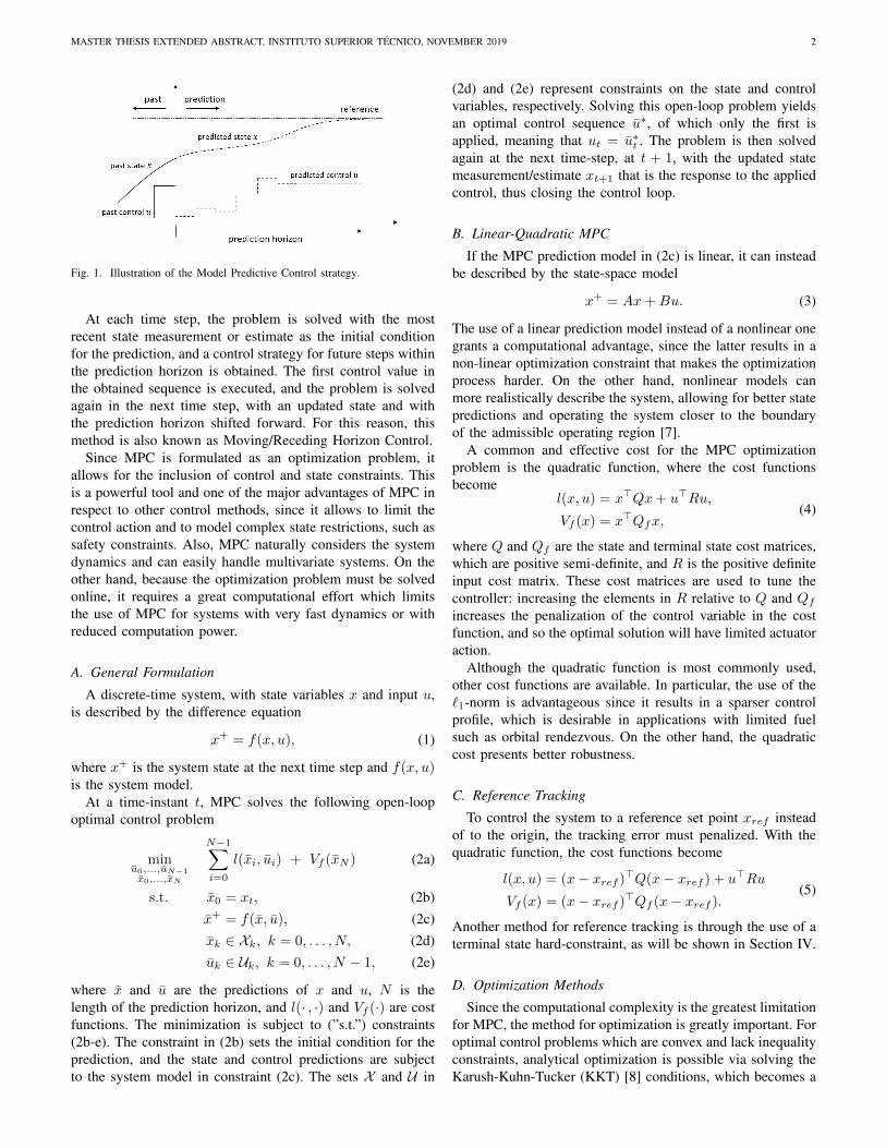
Fig. 2. The target local orbital frame (Flo).

spacecraft, respectively. Assuming an uniform gravitationalfield and that the the satellite masses are negligible, the relativemotion between the satellites is easily derived from Newton’slaw of gravitation and second law of motion, yielding

s = µ

(rtr3t

− rcr3c

)+

F

mc, (6)

where µ is the standard gravitational parameter, F is the forceapplied by the chaser thrusters, and mc is the chaser mass.Unlike in the case of only one unperturbed satellite, thisproblem has no closed-form solution and must be solvednumerically or approximated with a linearisation.

A. Target Local Orbital Frame

When the distance between the two spacecraft is small, itis convenient to consider the non-inertial target local orbitalframe, illustrated in Fig. 2, where θ is the true anomalyof the target spacecraft. This frame is also known as local-vertical/local-horizontal frame (LVLH), given that it is centredin the position of the target spacecraft.

Axis xlo is in the general direction of the velocity vector,although it is not always aligned with it, and is commonlyknown as V-bar. Axis ylo is orthogonal to the orbital plane,in the opposite direction of the angular momentum, and isalso known as H-bar. The axis zlo, known as R-bar, is alwaysdirected at the center of mass of the central body. For thisreason, the frame rotates with the orbital angular velocity ω,and thus is non-inertial.

B. Approximate Equations of Relative Motion

To make use of the nonlinear relative dynamics in (6), alinearisation is performed around the target position rt [1].Furthermore, the relative position is converted to the LVLHframe, yielding the linearised equations of relative motion(LERM)

x− ω2x− 2ωz − ωz + kω32x =

Fx

mc, (7a)

y + kω32 y =

Fy

mc, (7b)

z − ω2z + 2ωx+ ωx− 2kω32 z =

Fz

mc, (7c)

where (x, y, z) is chaser position relative to the target in theLVLH frame, F = [Fx, Fy, Fz]>, and k is the constant k =µ/h

32 , with h as the magnitude of the target orbit specific

angular momentum.


The LERM equations are linear with respect to relativeposition, velocity and acceleration, although they are not sowith respect to the orbital angular velocity ω. Because thisparameter is time-varying for elliptical orbits, in general theequations are linear and time-varying, and thus a solutionis not trivial. A special case emerges for a circular targetorbit, where the orbital angular velocity becomes constantwith time and thus the dynamics become time-invariant. Inthis case, the LERM equations become the well-known Hillequations, and their solution, known as the Clohessy-Wiltshireequations, is trivial. Finally, notice that the motion in H-bar,which is referred to as out-of-plane motion, is decoupledfrom that in V-bar and R-bar, designated in-plane motion.This simplifies the problem, since the two can be solved andanalysed independently. However, note that this is directly dueto the linearisation, and that in the nonlinear dynamics the twoare in fact coupled.

C. Simplification of the General Equations

To solve the LERM equations in the general elliptic orbitcase, a change of the independent variable from time t tothe true anomaly θ is employed. Furthermore, a coordinatetransformation is also applied

s = ρ(θ)s, (8)

where s is the relative position vector in the new coordinatesystem and ρ(θ) is a time-variant auxiliary function definedas

ρ(θ) = 1 + e cos(θ), (9)

where e is the orbit eccentricity. Denoting the derivative of swith respect to the true anomaly θ as s′, the transformationfor velocity is

s′ = −e sin(θ)s +1

k2ρ(θ)s. (10)

Applying these transformations, the LERM equations sim-plify to

x′′ − 2z′ =Fx

mck4ρ3, (11a)

y′′ + y =Fy

mck4ρ3, (11b)

z′′ − 3

ρz + 2x′ =

Fx

mck4ρ3, (11c)

which are known as the Tschauner–Hempel equations and canbe more easily solved.

D. Homogeneous Solution

For the homogeneous solution of the Tschauner–Hempelequations (F = 0), we consider the Yamanaka-Ankersen equa-tions [5]. Given initial conditions x0 = [x0, y0, z0, x

′0, y′0, z′0]>

for an initial true anomaly θ0, the homogeneous solutionbecomes

xh(θ) = φ(θ)φ−1(θ0)x0, (12)

where φ(θ) is a transition matrix not presented here for brevity.

E. Particular Solution

We will consider Ankersen’s particular solution [6], whichassumes a constant force during the sampling period andthus results in a zero-order hold (ZOH) discretization. Theparticular solution thus becomes

xp(θ) = Γ(θ0, θ)F, (13)

where input matrix Γ(θ0, θ) is also not presented here.

F. State-Space Model

Representing the coordinate transformations in (8) and (10)with the transformation matrix Λ(θ) and the inverse trans-formation with Λ−1(θ), we get the state-space model in theoriginal coordinates

xk+1 = Ak+1k xk +Bk+1

k uk, (14)

with the input vector u = F, and such that the system at adiscrete time k has true anomaly θ0 and at time k+ 1 the trueanomaly θ. Matrix Ak+1

k is the state transition matrix fromtime k to k + 1

Ak+1k = Λ−1(θ)φ(θ)φ−1(θ0)Λ(θ0), (15)

while Bk+1k is the input matrix, which becomes

Bk+1k = Λ−1(θ)Γ(θ0, θ). (16)

Given two arbitrary positions and a transfer duration, theYamanaka-Ankersen state transition matrix Ak+1

k can be usedto generate two-impulse manoeuvres, by solving for the initialand final changes in velocity required, designated ∆V ’s.These manoeuvres are often used to generate trajectories intraditional rendezvous guidance techniques.

IV. RENDEZVOUS WITH MPC

In traditional rendezvous mission design, guidance trajec-tories are designed offline, and so manoeuvres are performedin open-loop, often times with punctual mid-course correctionboosts determined online from the trajectory deviation. In thiscontext, an increasing amount of research has been dedicatedto applying Model Predictive Control (MPC) to the rendezvousproblem [12], in order to perform these thrust manoeuvresonline and in full closed-loop.

A. Relative Dynamics Sampling

The relative dynamics are time-varying for elliptical orbits,which presents a difficulty for the sampling of the MPCprediction horizon. For example, in the conditions of thePROBA-3 mission, the orbital velocity is nearly ten timesgreater at perigee than at apogee, which also translates to thevelocity of the relative motion. Because in MPC there is alimited amount of samples, associated with the length of theprediction horizon, these must be allocated appropriately alongthe orbit in order to get the best performance, since the pointat which the thrust is applied is important for the optimalityof the trajectory.

If the dynamics are sampled with constant time intervals,the samples will concentrate on apogee because the orbital


velocity is greater there, which is opposite to what is desiredsince the dynamics are faster on perigee. Thus, in this workwe sample the dynamics with constant eccentric anomaly in-tervals, which results in longer time intervals between samplesat apogee than at perigee, in way that samples are uniformlydistributed in space.

B. Fixed-Horizon MPC

The receding-horizon strategy which is standard for MPCis not appropriate for the rendezvous scenario. The fact thatthe prediction horizon slides forward every sample means thesystem can never commit to one specific trajectory, whichprohibits achieving a fuel-optimal closed-loop trajectory. Thus,the standard approach is to decrement the prediction horizonevery sample, such that its edge is always at the same time-instant, and thus known as Fixed-Horizon MPC (FH-MPC)[13].

To achieve a fuel-optimal formulation, the cost functionmust also be chosen appropriately. First, no intermediatecost l(· , ·) is used for the state variables, thus allowing thecontroller to better plan ahead since it is not penalized fornot being on the reference state while halfway through themanoeuvre. Also, for the input variable cost, the `1-norm isused. Because the absolute value of the thrust is proportionalto the fuel consumption, this cost function allows for thedirect minimization of the fuel required for the manoeuvre.On the other hand, the use of the `1-norm does not allow fora computationally efficient optimization.

To simplify the cost function, the input matrix in theprediction model can be extended, such that input forces aresplit into its positive and negative components F = F+−F−.This increases the number of optimization variables, whichis disadvantageous, but now each input variable can onlytake positive values, which makes its absolute value equal toitself, thus turning the `1-norm into a linear cost function. Tosimplify the problem further, the terminal state cost Vf (·) isremoved and replaced with a terminal state constraint, whichallows for the cost function to become completely linear. Thus,the standard FH-MPC formulation, as first presented in [13],becomes

minu0,...,uN−1x0,...,xN

N−1∑i=0

∆ti1>ui (17a)

s.t. x0 = xt, (17b)


k uk, (17c)0 ≤ uk ≤ umax, k = 0, . . . , N − 1, (17d)xN = xref , (17e)

which is a linear program (LP) and can be solved veryefficiently. Notice that in (17a) the input variables are weightedwith the time intervals between samples ∆t, which is im-portant to maintain the cost function proportional to the fuelrequired, since a ZOH discretization is used and the systemis not sampled with constant time intervals. Furthermore, theconstraint in (17d) limits the control to the maximum thrustumax, and also lower-bounds it with zero in order to maintainthe integrity of the input variable split. Finally, constraint (17e)

is the terminal state constraint, where xref is the referencestate. This constraint sets the manoeuvre duration, which isdefined by the prediction horizon N at the first iteration, andthus must be defined prior to the optimization.

C. Variable-Horizon MPC

It is also desirable to optimize the manoeuvre durationas well as fuel consumption, which is performed by addingthe prediction horizon N as an integer optimization variable,in what is known as Variable-Horizon MPC (VH-MPC).However, this makes the terminal constraint (17e) nonlinear,turning the problem intro a mixed-integer nonlinear program,which is computationally expensive to solve.

A method for transforming the problem into a mixed-integerlinear program (MILP) presented in [13] requires two binaryoptimization variables per time-instant. Variable vk is 1 if themanoeuvre is completed exactly at instant k, while pk is 1while the manoeuvre is not completed and 0 afterwards. TheVH-MPC MILP formulation then becomes

minu0,...,uNmax−1x0,...,xNmax

p0,...,pNmax∈{0,1}v1,...,vNmax∈{0,1}

γ

Nmax∑i=0

pi +

Nmax−1∑i=0

∆ti1>ui (18a)

s.t. x0 = xt, (18b)


k uk, (18c)0 ≤ uk ≤ umax, (18d)− (1− vk)h ≤ xk − xref ≤ (1− vk)h,

(18e)pk+1 = pk − vk+1, (18f)pNmax = 0, (18g)Nmax∑k=1

vk = 1. (18h)

where the new term in the cost function is proportional toN , and thus γ is a parameter used to tune the trade-offbetween fuel consumption and manoeuvre duration, whileNmax defines the maximum manoeuvre duration possible.Constraint (18e) is the new terminal state constraint, whereh is a large enough number; at the instant the manoeuvreis completed, vk is 1 and thus the terminal state constraint isactive, otherwise vk is 0 and the constraint is loose. Constraints(18f) and (18h) maintain the integrity of the binary variables,while (18g) forces the manoeuvre to be completed at least bythe end of the maximum prediction horizon.

The computational load for this formulation is greater thanfor the FH-MPC, since MILP problems are harder to solve.Thus, in a real-time scenario, it is preferable to predetermineoffline the manoeuvre duration and use the FH-MPC formu-lation instead. However determining the manoeuvre durationoffline can be performed in an optimal way by using theVH-MPC formulation. The optimal transfer time may changeslightly along the way due to disturbances, but the time de-termined offline can still be expected to remain approximatelyoptimal.


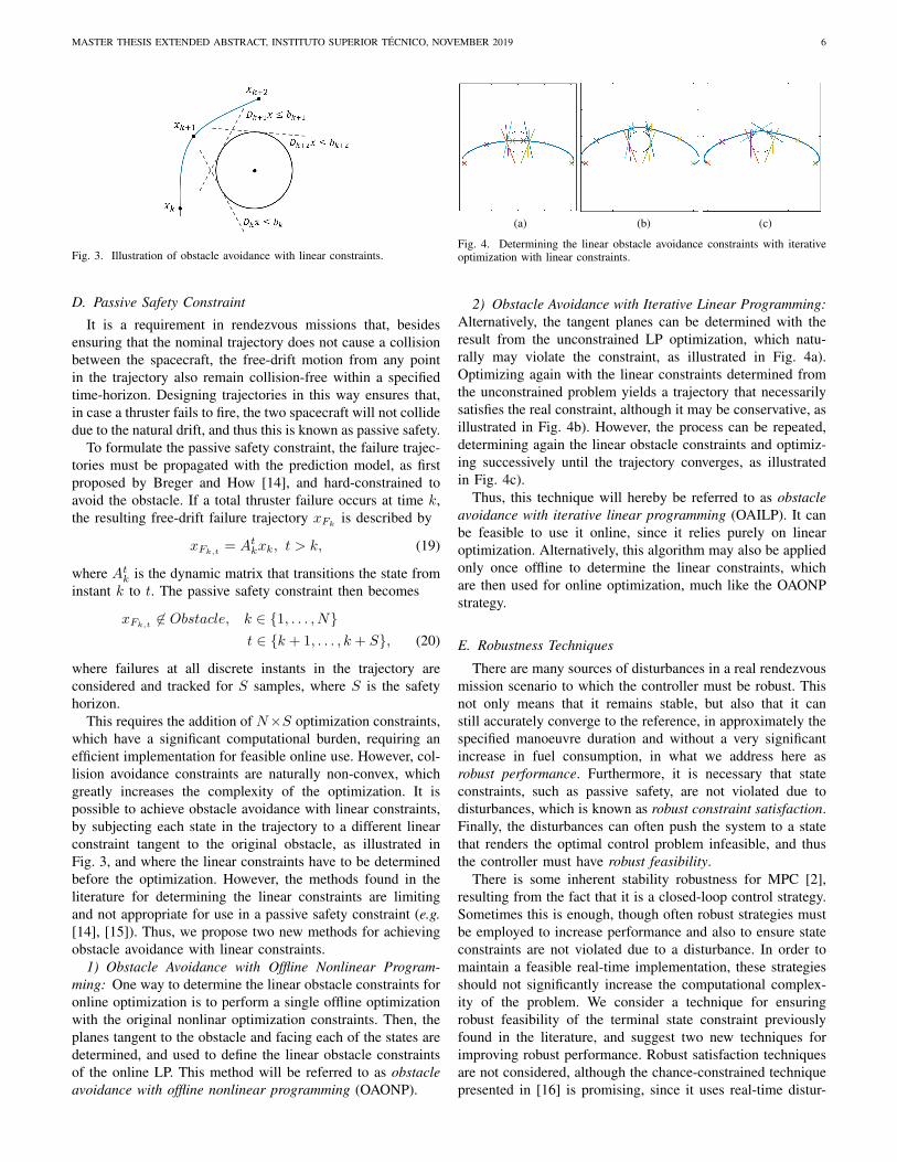
Fig. 3. Illustration of obstacle avoidance with linear constraints.

D. Passive Safety Constraint

It is a requirement in rendezvous missions that, besidesensuring that the nominal trajectory does not cause a collisionbetween the spacecraft, the free-drift motion from any pointin the trajectory also remain collision-free within a specifiedtime-horizon. Designing trajectories in this way ensures that,in case a thruster fails to fire, the two spacecraft will not collidedue to the natural drift, and thus this is known as passive safety.

To formulate the passive safety constraint, the failure trajec-tories must be propagated with the prediction model, as firstproposed by Breger and How [14], and hard-constrained toavoid the obstacle. If a total thruster failure occurs at time k,the resulting free-drift failure trajectory xFk

is described by

xFk,t= At

kxk, t > k, (19)

where Atk is the dynamic matrix that transitions the state from

instant k to t. The passive safety constraint then becomes

xFk,t6∈ Obstacle, k ∈ {1, . . . , N}

t ∈ {k + 1, . . . , k + S}, (20)

where failures at all discrete instants in the trajectory areconsidered and tracked for S samples, where S is the safetyhorizon.

This requires the addition of N×S optimization constraints,which have a significant computational burden, requiring anefficient implementation for feasible online use. However, col-lision avoidance constraints are naturally non-convex, whichgreatly increases the complexity of the optimization. It ispossible to achieve obstacle avoidance with linear constraints,by subjecting each state in the trajectory to a different linearconstraint tangent to the original obstacle, as illustrated inFig. 3, and where the linear constraints have to be determinedbefore the optimization. However, the methods found in theliterature for determining the linear constraints are limitingand not appropriate for use in a passive safety constraint (e.g.[14], [15]). Thus, we propose two new methods for achievingobstacle avoidance with linear constraints.

1) Obstacle Avoidance with Offline Nonlinear Program-ming: One way to determine the linear obstacle constraints foronline optimization is to perform a single offline optimizationwith the original nonlinar optimization constraints. Then, theplanes tangent to the obstacle and facing each of the states aredetermined, and used to define the linear obstacle constraintsof the online LP. This method will be referred to as obstacleavoidance with offline nonlinear programming (OAONP).

(a) (b) (c)

Fig. 4. Determining the linear obstacle avoidance constraints with iterativeoptimization with linear constraints.

2) Obstacle Avoidance with Iterative Linear Programming:Alternatively, the tangent planes can be determined with theresult from the unconstrained LP optimization, which natu-rally may violate the constraint, as illustrated in Fig. 4a).Optimizing again with the linear constraints determined fromthe unconstrained problem yields a trajectory that necessarilysatisfies the real constraint, although it may be conservative, asillustrated in Fig. 4b). However, the process can be repeated,determining again the linear obstacle constraints and optimiz-ing successively until the trajectory converges, as illustratedin Fig. 4c).

Thus, this technique will hereby be referred to as obstacleavoidance with iterative linear programming (OAILP). It canbe feasible to use it online, since it relies purely on linearoptimization. Alternatively, this algorithm may also be appliedonly once offline to determine the linear constraints, whichare then used for online optimization, much like the OAONPstrategy.

E. Robustness Techniques

There are many sources of disturbances in a real rendezvousmission scenario to which the controller must be robust. Thisnot only means that it remains stable, but also that it canstill accurately converge to the reference, in approximately thespecified manoeuvre duration and without a very significantincrease in fuel consumption, in what we address here asrobust performance. Furthermore, it is necessary that stateconstraints, such as passive safety, are not violated due todisturbances, which is known as robust constraint satisfaction.Finally, the disturbances can often push the system to a statethat renders the optimal control problem infeasible, and thusthe controller must have robust feasibility.

There is some inherent stability robustness for MPC [2],resulting from the fact that it is a closed-loop control strategy.Sometimes this is enough, though often robust strategies mustbe employed to increase performance and also to ensure stateconstraints are not violated due to a disturbance. In order tomaintain a feasible real-time implementation, these strategiesshould not significantly increase the computational complex-ity of the problem. We consider a technique for ensuringrobust feasibility of the terminal state constraint previouslyfound in the literature, and suggest two new techniques forimproving robust performance. Robust satisfaction techniquesare not considered, although the chance-constrained techniquepresented in [16] is promising, since it uses real-time distur-


bance estimation for constraint-tightening and maintains theoptimization problem as an LP.

1) Feasible Terminal Box: When the prediction horizonbecomes short, as it does with the FH strategy, disturbancescan push the system to a state from which the referenceis not reachable in the remaining steps, given the systemdynamics and other control and state constraints. This rendersthe terminal state constraint and the optimization probleminfeasible, which should be avoided at all costs in a real-timeapplication.

This can be minimized by relaxing the terminal stateconstraint into an inequality, thus introducing the concept ofterminal box. The terminal constraint (17e) then becomes

−δ ≤ xN − xref ≤ δ, (21)

where δ ∈ R6 defines the bounds for the box. However,improving the guarantee of feasibility requires increasing thesize of the terminal box, which in turn this worsens theaccuracy of the controller. Furthermore, there is no guaranteethat the chosen dimensions for the terminal box will alwaysensure the existence of a solution for all possible scenarios.

To improve this approach, the box bounds δ can be in-cluded as optimization variables, as first suggested in [17],which maintains the constraint linear. Furthermore, the newoptimization variables are included in the cost function

V (·) =

N−1∑i=0

∆ti1>ui +

6∑j=1

hjδj , (22)

where hj is large enough as to ensure the controller onlyrelaxes the terminal constraint to ensure feasibility and notto save fuel. Thus, this feasible terminal box will always havethe minimum size that guarantees feasibility.

2) Dynamic Terminal Box: The terminal state constraintforces the controller to set the fate state exactly on thereference at every iteration. In the presence of stochasticdisturbances, however, this may cause an overcorrection ofthe trajectory and results in the waste of propellant. This maybe minimized by loosening the terminal box, allowing thecontroller to perform fewer corrections, although at the costof decreased manoeuvre accuracy.

Thus, we propose the inclusion of a time-varying bound εtto the terminal box constraint

−δ − εt ≤ xN − xref ≤ δ + εt, (23)

where t is the time instant at which the optimization problemis being solved. The bound εt is decreased with time, suchthat it reduces the controller overcorrection but still maintainsaccuracy as it approaches the reference. This technique is notmutually exclusive with the feasible terminal box method.

3) Terminal Quadratic Controller: The sparse thrust profileof the FH-MPC formulation is not appropriate for executingaccurate manoeuvres in the presence of disturbances, sincecrucial ∆V ’s are performed in one sample only, while plan-ning under imperfect state information and with imperfectexecution of the ∆V . Thus the final braking thrust at the endof manoeuvres for cancelling the remaining relative velocity

tends to not be very precise, resulting in a poor manoeuvreaccuracy.

Therefore, we propose the use of a linear-quadratic MPCcontroller, such as that in (5), to substitute the final sampleof the FH-MPC and perform the final breaking thrust. Theterminal controller has a prediction horizon NT that has thesame timespan as the last sample of the nominal controller andis decremented in the same FH strategy, in order to maintainthe manoeuvre duration initially specified. Furthermore, aterminal state cost is used instead of the terminal constraint,and the intermediate state cost is zero. The non-sparse thrustprofile resulting from the use of the quadratic cost and theincreased control decisions result in a more accurate brakingmanoeuvre.

V. EXPERIMENTS AND RESULTS

This section features several rendezvous simulations withthe techniques presented. Simulations are performed for Earthsatellites, with the perigee height and chaser mass for thePROBA-3 RVX of 600 km and 211 kg, respectively. The orbiteccentricity e simulated is either 0, for experiments in circularorbits, or with the PROBA-3 eccentricity of 0.8111. The initialtrue anomaly θ0 is indicated for elliptical orbit experiments,and is irrelevant for circular orbits. The orbital orientationparameters are disregarded, since a uniform gravitational is as-sumed. For circular orbits, the sampling period Ts is presented,while for elliptical orbits the sampling eccentric anomaly Es

is shown. Finally, the fuel expenditure is analysed via the total∆V applied by the chaser thrusters, which have a max thrustof 1 N in each direction.

The MPC optimization problem is solved with theMATLAB Optimization Toolbox, where function linprog isused for linear programming for the FH-MPC formulation,function intlinprog is used to solve the MILP in the VH-MPCformulation, and fmincon is used for solving the nonlinearprogram that arises in the OAONP technique. Because these al-gorithms do not take advantage of the MPC problem structure,the state-substitution technique briefly mentioned in SectionII-D is utilized. The worst-case computation times tmax forsolving the optimization problem is presented, solving with a4th Generation 2.4GHz Intel-i7 Processor.

A. FH-MPC

Applying the FH-MPC controller to a V-bar transfer sce-nario with an initial prediction horizon of just over one orbitalperiod yields the result from Fig. 5, where the manoeuvre isperformed with only two V-bar thrust actions. This resemblesthe ideal V-bar transfer with two horizontal impulses [1], forwhich the required ∆V exactly matches that obtained in thisexperiment. Thus, this validates the fuel-optimality of the FH-MPC formulation. The computation time was 7.97 ms in theworst case, which is very small comparing to the samplingtime.

Considering an elliptical orbit and including the H-bardimension, we simulate a manoeuvre from the PROBA-3RVX, which starts approximately at apogee and ends nearperigee. The ∆V required to perform this manoeuvre with the


(a) (b)

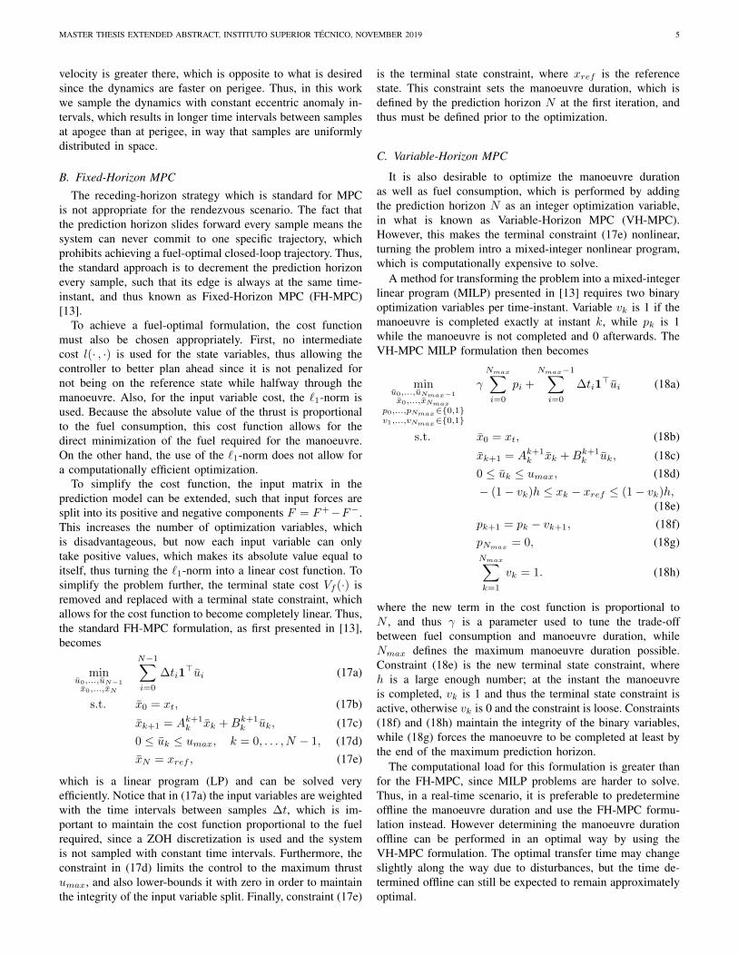
Fig. 5. V-bar transfer manoeuvre in one orbital period with FH-MPC. (a)Trajectory (b) State and control variables. Simulation parameters: N = 21,Ts = 290 s. Results: ∆V = 3.45 mm/s, tmax = 7.97 ms.

(a) (b)

Fig. 6. Manoeuvre from the PROBA-3 RVX with FH-MPC. (a) Trajectory(b) State and control variables. Simulation parameters: N = 100, Es =1.70 deg, θ0 = 179 deg. Results: ∆V = 407.4 mm/s, tmax = 9.52 ms.

traditional two-impulse transfer is 481 mm/s, while FH-MPCyields a manoeuvre with 407 mm/s, thus requiring only 85%of the fuel that would typically be expended. This is possibledue to the fact that the traditional two-impulse manoeuvresare constrained to one thrust action at beginning and anotherat end of the manoeuvre, while MPC may take intermediatecontrol decisions. Thus, via the intermediate thrust actionseen in H-bar toward the end, a more efficient manoeuvre ispossible, which further shows the fuel-optimality of the FH-MPC formulation. Finally, notice that despite the fact that thethe prediction horizon was increased by almost five times,the worst-case computation time only increased by 19.4%,thus demonstrating the benefit of formulating the optimizationproblem as a linear program.

B. VH-MPC

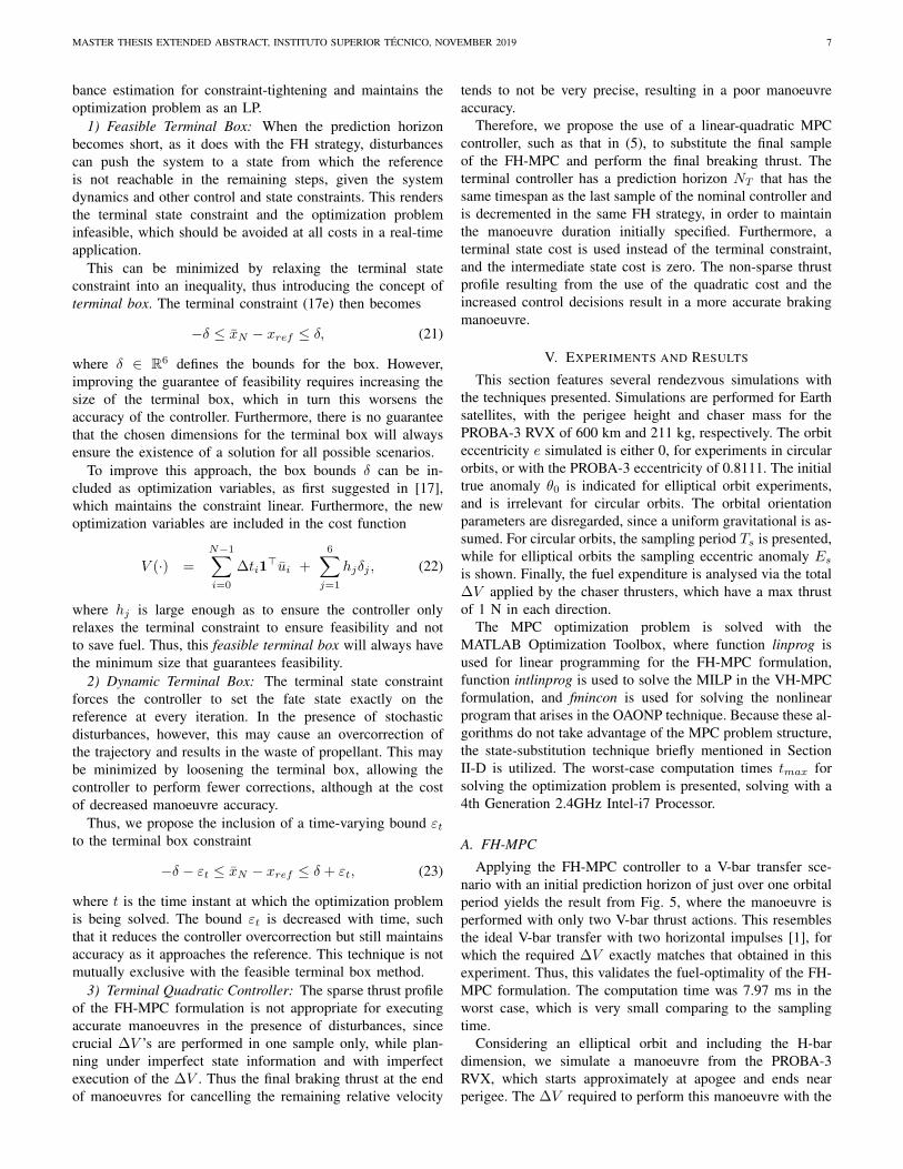
Applying now the VH-MPC formulation to the previousPROBA-3 manoeuvre with a maximum transfer time of oneorbital period yields the result from Fig. 7. Parameter γ isset to zero in order to only minimize the required fuel. Theoptimal transfer time obtained is 41% of an orbital period,yielding a ∆V of 48.16 mm/s, which is only 11.8% as thatrequired for the half-orbit transfer in Fig. 6, thus validating theVH-MPC formulation. However, a transfer time of one orbitalperiod would actually have been even more efficient, and iswithin the maximum duration specified. The reason VH-MPCdid not yield that solution is that the ∆V is not a convexfunction of the transfer time, and the algorithm used to solvethe MILP does not optimize globally, and thus it converges tothis local minimum.

(a) (b)

Fig. 7. Manoeuvre from the PROBA-3 RVX with VH-MPC. (a) Trajectory(b) State and control variables. Simulation parameters: Nmax = 100, γ = 0,Es = 3.6 deg, θ0 = 179 deg. Results: N = 41, ∆V = 48.16 mm/s,tmax = 710 ms.

(a) (b)

Fig. 8. V-bar transfer manoeuvre in one orbital period with FH-MPC andpassive safety constraint with OAONP. (a) Trajectory (b) State and controlvariables. Controller parameters: N = 30, Ts = 193 s, S = 30. Simulationresults: ∆V = 1.62 mm/s, tmax = 21.7 ms, toffline = 1.31 s.

Finally, notice that the worst-case computation time requiredto solve the MILP is significantly greater than that of the LPin the FH-MPC formulation. Therefore, it may be infeasible touse the VH-MPC formulation online, especially with the in-clusion of the computationally heavy passive safety constraint.

C. Passive Safety

Considering passive safety, Fig. 8 presents the same typeof V-bar transfer manoeuvre presented previously in Fig. 5with the inclusion of this constraint with a one-orbit safetyhorizon, formulated with the OAONP technique. Without it, athruster failure in the final burn would result in a violation ofthe target safety region, defined here as a 2 metre circle, afterless than an orbit. With the passive safety constraint, someextra actuation at the end of the manoeuvre ensures that thefailure trajectories stop at the edge of the safety region exactlyafter one orbital period.

This comes at the cost of a 17% increase in fuel with respectto the non-passively safe trajectory. Furthermore, the computa-tion time for optimizing with the nonlinear constraints is 1.31s. However, the OAONP technique allows for this optimizationto be performed just once offline, and the online computationtime, although having increased due to the addition of 900linear optimization constraints, remains 2 orders of magnitudesmaller than this.

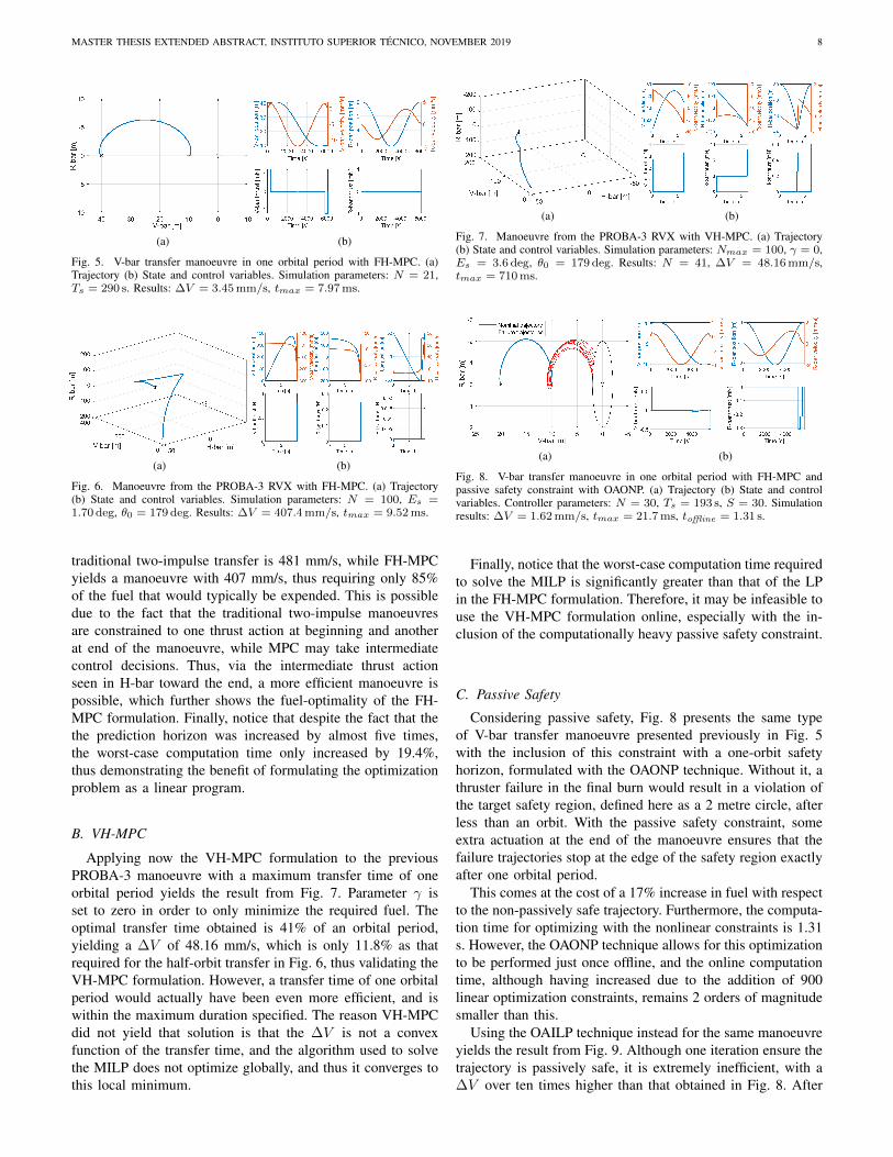
Using the OAILP technique instead for the same manoeuvreyields the result from Fig. 9. Although one iteration ensure thetrajectory is passively safe, it is extremely inefficient, with a∆V over ten times higher than that obtained in Fig. 8. After


(a) (b) (c)

Fig. 9. V-bar transfer manoeuvre in one orbital period with FH-MPC and pas-sive safety constraint with OAILP. (a) One iteration, ∆V = 20.76 mm/s (b)Two iterations, ∆V = 2.039 mm/s (c) Three iterations, ∆V = 1.62 mm/s.Controller parameters: N = 30, Ts = 193 s, S = 30. Simulation results:tmax = 17.8 ms, toffline = 212.4 ms.

two iterations the result improves drastically, although the ∆Vis still above the optimal trajectory. With three iterations theresult almost exactly matches that with the previous method,and the ∆V is also approximately the same. Similarly to theOAONP strategy, the OAILP algorithm was run only onceoffline, and the computation time is significantly less than theformer.

The satisfaction of non-convex obstacle avoidance constraintvia purely linear constraints is promising and desirable, al-though there currently is no guarantee that the trajectory con-verges to a local minimum of the original nonlinear problem,which warrants further research.

D. Robustness Experiments

So far simulations have been performed with the samelinearised model used for the MPC prediction model, andthus there are no modelling errors. Simulating the PROBA-3manoeuvre with the real nonlinear dynamics yields the resultfrom Fig. 10. The trajectory is slightly different from thatobtained in Fig. 6, with some extra actuation at the end ofthe manoeuvre in an attempt to correct the disturbance thatresults in an increase of the ∆V of 22%. Furthermore, thefeasible terminal box technique from Section IV-E1 is applied,having no significant increase in computational time, otherwisethe last iteration would become infeasible and the manoeuvreincomplete. There is also a residual deviation of the final statefrom the reference in position epos and velocity evel, dueto the loosening of the terminal constraint and the imperfectprecision model. While increasing the number of samples inthe prediction horizon decreases this error and the ∆V , suchan approach is not effective in the presence of stochasticdisturbances.

We now consider an additive Gaussian error to the statereceived by the controller with a standard deviation of 10cm for position and 1 mm/s for velocity, thus modellingnavigation errors. Also, an error in thrust magnitude with astandard deviation of 10% and in orientation of 0.5 deg ineach direction is applied, modelling thruster errors. Finally,control commands under 1 mN are ignored in order to modelthe minimum thrust possible via pulse-width modulation of theon/off thrusters. Because the conditions are now stochastic, 20simulations are performed and the results averaged. In theseconditions yields the result from Fig. 11.

(a) (b)

Fig. 10. Manoeuvre from the PROBA-3 RVX with FH-MPC with feasibleterminal box and simulated with the nonlinear dynamics. (a) Trajectory(b) State and control variables. Simulation parameters: N = 100, Es =1.70 deg, θ0 = 179 deg. Results: ∆V = 497.5 mm/s, tmax = 10.1 ms,epos = 25.44 cm, evel = 4.746mm/s.

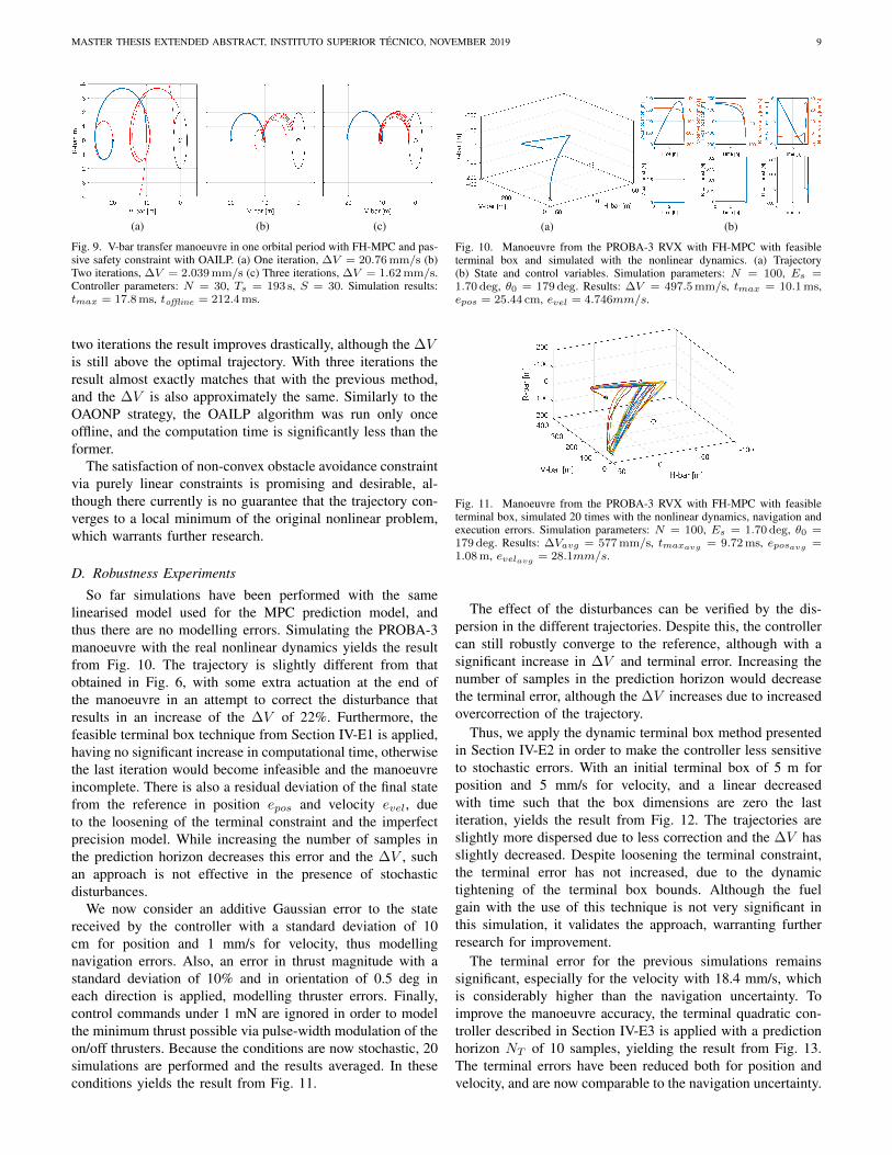
Fig. 11. Manoeuvre from the PROBA-3 RVX with FH-MPC with feasibleterminal box, simulated 20 times with the nonlinear dynamics, navigation andexecution errors. Simulation parameters: N = 100, Es = 1.70 deg, θ0 =179 deg. Results: ∆Vavg = 577 mm/s, tmaxavg = 9.72 ms, eposavg =1.08 m, evelavg = 28.1mm/s.

The effect of the disturbances can be verified by the dis-persion in the different trajectories. Despite this, the controllercan still robustly converge to the reference, although with asignificant increase in ∆V and terminal error. Increasing thenumber of samples in the prediction horizon would decreasethe terminal error, although the ∆V increases due to increasedovercorrection of the trajectory.

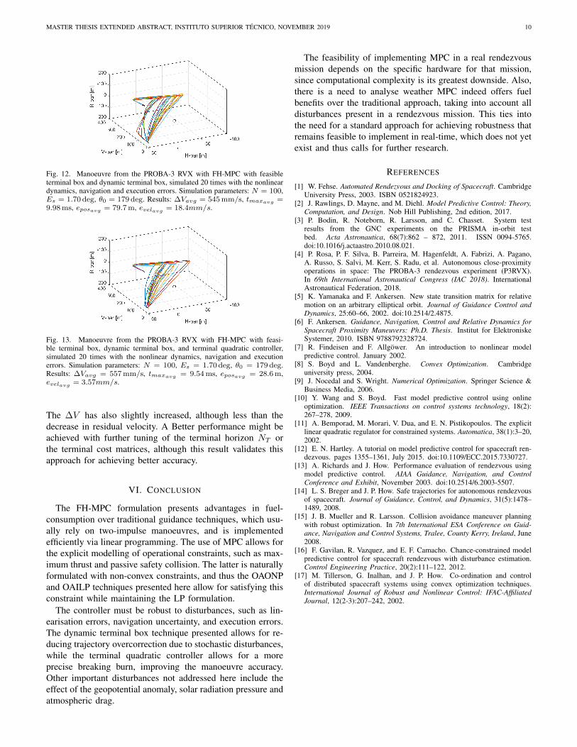
Thus, we apply the dynamic terminal box method presentedin Section IV-E2 in order to make the controller less sensitiveto stochastic errors. With an initial terminal box of 5 m forposition and 5 mm/s for velocity, and a linear decreasedwith time such that the box dimensions are zero the lastiteration, yields the result from Fig. 12. The trajectories areslightly more dispersed due to less correction and the ∆V hasslightly decreased. Despite loosening the terminal constraint,the terminal error has not increased, due to the dynamictightening of the terminal box bounds. Although the fuelgain with the use of this technique is not very significant inthis simulation, it validates the approach, warranting furtherresearch for improvement.

The terminal error for the previous simulations remainssignificant, especially for the velocity with 18.4 mm/s, whichis considerably higher than the navigation uncertainty. Toimprove the manoeuvre accuracy, the terminal quadratic con-troller described in Section IV-E3 is applied with a predictionhorizon NT of 10 samples, yielding the result from Fig. 13.The terminal errors have been reduced both for position andvelocity, and are now comparable to the navigation uncertainty.


Fig. 12. Manoeuvre from the PROBA-3 RVX with FH-MPC with feasibleterminal box and dynamic terminal box, simulated 20 times with the nonlineardynamics, navigation and execution errors. Simulation parameters: N = 100,Es = 1.70 deg, θ0 = 179 deg. Results: ∆Vavg = 545 mm/s, tmaxavg =9.98 ms, eposavg = 79.7 m, evelavg = 18.4mm/s.

Fig. 13. Manoeuvre from the PROBA-3 RVX with FH-MPC with feasi-ble terminal box, dynamic terminal box, and terminal quadratic controller,simulated 20 times with the nonlinear dynamics, navigation and executionerrors. Simulation parameters: N = 100, Es = 1.70 deg, θ0 = 179 deg.Results: ∆Vavg = 557 mm/s, tmaxavg = 9.54 ms, eposavg = 28.6 m,evelavg = 3.57mm/s.

The ∆V has also slightly increased, although less than thedecrease in residual velocity. A Better performance might beachieved with further tuning of the terminal horizon NT orthe terminal cost matrices, although this result validates thisapproach for achieving better accuracy.

VI. CONCLUSION

The FH-MPC formulation presents advantages in fuel-consumption over traditional guidance techniques, which usu-ally rely on two-impulse manoeuvres, and is implementedefficiently via linear programming. The use of MPC allows forthe explicit modelling of operational constraints, such as max-imum thrust and passive safety collision. The latter is naturallyformulated with non-convex constraints, and thus the OAONPand OAILP techniques presented here allow for satisfying thisconstraint while maintaining the LP formulation.

The controller must be robust to disturbances, such as lin-earisation errors, navigation uncertainty, and execution errors.The dynamic terminal box technique presented allows for re-ducing trajectory overcorrection due to stochastic disturbances,while the terminal quadratic controller allows for a moreprecise breaking burn, improving the manoeuvre accuracy.Other important disturbances not addressed here include theeffect of the geopotential anomaly, solar radiation pressure andatmospheric drag.

The feasibility of implementing MPC in a real rendezvousmission depends on the specific hardware for that mission,since computational complexity is its greatest downside. Also,there is a need to analyse weather MPC indeed offers fuelbenefits over the traditional approach, taking into account alldisturbances present in a rendezvous mission. This ties intothe need for a standard approach for achieving robustness thatremains feasible to implement in real-time, which does not yetexist and thus calls for further research.

REFERENCES

[1] W. Fehse. Automated Rendezvous and Docking of Spacecraft. CambridgeUniversity Press, 2003. ISBN 0521824923.

[2] J. Rawlings, D. Mayne, and M. Diehl. Model Predictive Control: Theory,Computation, and Design. Nob Hill Publishing, 2nd edition, 2017.

[3] P. Bodin, R. Noteborn, R. Larsson, and C. Chasset. System testresults from the GNC experiments on the PRISMA in-orbit testbed. Acta Astronautica, 68(7):862 – 872, 2011. ISSN 0094-5765.doi:10.1016/j.actaastro.2010.08.021.

[4] P. Rosa, P. F. Silva, B. Parreira, M. Hagenfeldt, A. Fabrizi, A. Pagano,A. Russo, S. Salvi, M. Kerr, S. Radu, et al. Autonomous close-proximityoperations in space: The PROBA-3 rendezvous experiment (P3RVX).In 69th International Astronautical Congress (IAC 2018). InternationalAstronautical Federation, 2018.

[5] K. Yamanaka and F. Ankersen. New state transition matrix for relativemotion on an arbitrary elliptical orbit. Journal of Guidance Control andDynamics, 25:60–66, 2002. doi:10.2514/2.4875.

[6] F. Ankersen. Guidance, Navigation, Control and Relative Dynamics forSpacecraft Proximity Maneuvers: Ph.D. Thesis. Institut for ElektroniskeSystemer, 2010. ISBN 9788792328724.

[7] R. Findeisen and F. Allgower. An introduction to nonlinear modelpredictive control. January 2002.

[8] S. Boyd and L. Vandenberghe. Convex Optimization. Cambridgeuniversity press, 2004.

[9] J. Nocedal and S. Wright. Numerical Optimization. Springer Science &Business Media, 2006.

[10] Y. Wang and S. Boyd. Fast model predictive control using onlineoptimization. IEEE Transactions on control systems technology, 18(2):267–278, 2009.

[11] A. Bemporad, M. Morari, V. Dua, and E. N. Pistikopoulos. The explicitlinear quadratic regulator for constrained systems. Automatica, 38(1):3–20,2002.

[12] E. N. Hartley. A tutorial on model predictive control for spacecraft ren-dezvous. pages 1355–1361, July 2015. doi:10.1109/ECC.2015.7330727.

[13] A. Richards and J. How. Performance evaluation of rendezvous usingmodel predictive control. AIAA Guidance, Navigation, and ControlConference and Exhibit, November 2003. doi:10.2514/6.2003-5507.

[14] L. S. Breger and J. P. How. Safe trajectories for autonomous rendezvousof spacecraft. Journal of Guidance, Control, and Dynamics, 31(5):1478–1489, 2008.

[15] J. B. Mueller and R. Larsson. Collision avoidance maneuver planningwith robust optimization. In 7th International ESA Conference on Guid-ance, Navigation and Control Systems, Tralee, County Kerry, Ireland, June2008.

[16] F. Gavilan, R. Vazquez, and E. F. Camacho. Chance-constrained modelpredictive control for spacecraft rendezvous with disturbance estimation.Control Engineering Practice, 20(2):111–122, 2012.

[17] M. Tillerson, G. Inalhan, and J. P. How. Co-ordination and controlof distributed spacecraft systems using convex optimization techniques.International Journal of Robust and Nonlinear Control: IFAC-AffiliatedJournal, 12(2-3):207–242, 2002.

Documents

Design and Application of Thrust Manoeuvres in a