Embed Size (px)
Citation preview
Faculty of EngineeringDepartment of Electrical Energy, Systems and Automation
Head of Department: Prof. dr. ir. Jan Melkebeek
Design and Advanced Control of a
Process with Variable Time Delay
Steven HimpeVincent Theunynck
Promoter: Prof. dr. ir. Robin De KeyserThesis guide: ir. Mihaela Sbarciog
Master’s thesis submitted to obtain the degree of Civil Engineer in Mechanics andElectrotechnics
Academic Year 2005-2006

i
Permission to loan
The authors give permission to make this thesis available for consultation and to copy partsfor personal use. Any other use is covered by the restrictions of copyright, specially withrespect to the obligation to mention the source explicitly while quoting results or conclusionsfrom this thesis.
Steven Himpe Vincent Theunynck 1 June 2006
Preface
One year ago, the word ‘thesis’ still had something mythical, but now, here it is. For monthswe have been shaping it, questioning it and fostering it. Today, we are proud of it.
It was a pleasure to work on this subject as it challenged us on various fields. From thecontrol engineering point of view, since variable time delay problems are not easily addressedwith today’s most common controllers. From the practical point of view, as the process hadto be designed and realized. And, finally, from the personal point of view, since it took a lotof effort and perseverance to take the thesis to what it is now. Practice never lies.
We aimed to shape and structure this thesis to lead you along the different phases we walkedthrough, the numerous problems and challenges we experienced, and the solutions we con-trived. At the same time we hope to contribute our mite to the research on and improvementof controllers for processes with variable time delay.
Despite our enthusiasm, the final realization would not have been possible without the helpof a few persons, to whom we owe our thanks:our promoter, Prof. dr. ir. R. De Keyser, for giving the opportunity to do research on suchan interesting subject, for his proposals and suggestions to solve the more difficult problemswe experienced;our thesis guide, ir. Mihaela Sbarciog for her daily guidance, her effort, her support and herenthusiasm, for providing us with the tools we desperately needed, for the useful tips she gaveus and for the correction of the text;and Prof. dr. S. Cristea, for her interest in our thesis.
We also have to thank a lot of other people who made a contribution in one or another way.In particular our special thanks to Mr. Pascal Ghyselbrecht for helping us with the designand the selection of appropriate devices, for his crucial tips and for guiding us through thepractical implementation; and to Mr. Marc Deboeck from Lameco NV for his patience evenafter numerous phone calls, for his support in the search for a suitable pump and for hisspecial effort to make it affordable.
And finally, to our parents, our family and our friends: thanks a lot for your support !
ii
Survey
Design and Advanced Control of a Process with Variable Time Delay
bySteven Himpe and Vincent Theunynck
Master’s thesis submitted to obtain the degree of Civil Engineer in Mechanics andElectrotechnics, option Control Engineering and Automation
Academic Year 2005-2006
University of GhentFaculty of Engineering
Promoter: Prof. dr. ir. Robin De KeyserThesis Guide: ir. Mihaela Sbarciog
Summary
In this thesis a test setup for a process with variable time delay is designed and implemented.The process under consideration is a heating tank whose water temperature has to be con-trolled. A constant heat input is provided by a heater which causes the water to warm up.The actual control is done via an adjustable inflow of cold tap water while an equal outflowof hot water is removed from the tank in order to have a constant volume. The variabletime delay is obtained by measuring the temperature in the outlet tube, at a certain distancefrom the tank instead of in the tank itself. After the construction of the plant, an advancedcontroller of the MPC-type (Model Based Predictive Control) is programmed.The first part of this thesis discusses the design and implementation of the setup. The secondpart handles the advanced controller and research is done on how to adjust the MPC-controllerto deal with the variable time delay problem.
Keywords: Variable time delay, non-linear process, Model Based Predictive Control (MPC),Non-linear Extended Prediction Self-Adaptive Control (NEPSAC), Smith predictor, PI-controller
iii

Extended abstract
(English and Dutch version)
iv
Design and Advanced Control of a Processwith Variable Time Delay
Steven Himpe, Vincent Theunynck
Supervisor(s): Prof. dr. ir. R. De Keyser
Abstract—This article handles on one hand the design and implementa-tion of a setup to create a process with variable time delay, and on the otherhand an advanced control strategy for it, using a model predictive control(MPC) approach developed at Ghent University: EPSAC (Extended Pre-diction Self-Adaptive Control).
Keywords—variable time delay, MPC, EPSAC, Smith predictor
I. INTRODUCTION
VARIABLE time delay processes pose a challenging prob-lem in control engineering. A time delay of the order of the
time constant of the system, combined with a variation of it, re-quires an inventive control strategy to fullfil certain performancerequirements. As there are many practical problems involvingvariable time delay in industry (e.g. steel rolling processes orpaper manufacturing), it would be interesting to have an exper-imental setup with variable time delay, to test and develop newcontrol strategies on it.
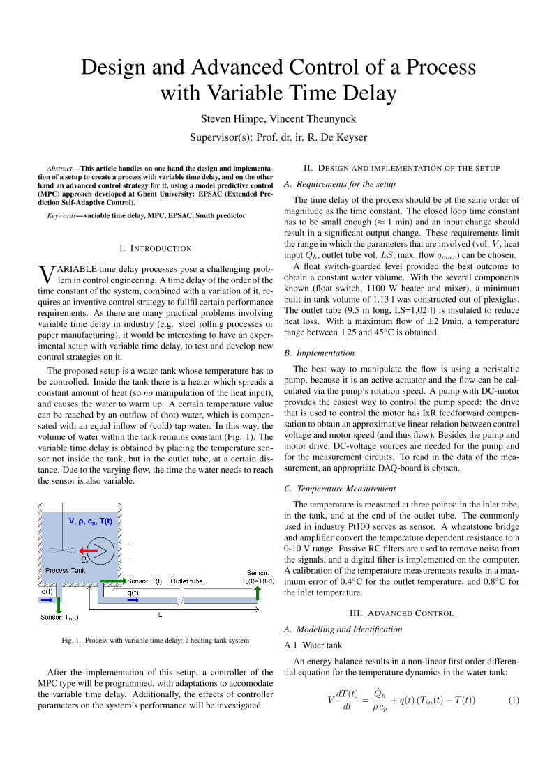
The proposed setup is a water tank whose temperature has tobe controlled. Inside the tank there is a heater which spreads aconstant amount of heat (so no manipulation of the heat input),and causes the water to warm up. A certain temperature valuecan be reached by an outflow of (hot) water, which is compen-sated with an equal inflow of (cold) tap water. In this way, thevolume of water within the tank remains constant (Fig. 1). Thevariable time delay is obtained by placing the temperature sen-sor not inside the tank, but in the outlet tube, at a certain dis-tance. Due to the varying flow, the time the water needs to reachthe sensor is also variable.
Fig. 1. Process with variable time delay: a heating tank system
After the implementation of this setup, a controller of theMPC type will be programmed, with adaptations to accomodatethe variable time delay. Additionally, the effects of controllerparameters on the system’s performance will be investigated.
II. DESIGN AND IMPLEMENTATION OF THE SETUP
A. Requirements for the setup
The time delay of the process should be of the same order ofmagnitude as the time constant. The closed loop time constanthas to be small enough (≈ 1 min) and an input change shouldresult in a significant output change. These requirements limitthe range in which the parameters that are involved (vol. V , heatinput Qh, outlet tube vol. LS, max. flow qmax) can be chosen.
A float switch-guarded level provided the best outcome toobtain a constant water volume. With the several componentsknown (float switch, 1100 W heater and mixer), a minimumbuilt-in tank volume of 1.13 l was constructed out of plexiglas.The outlet tube (9.5 m long, LS=1.02 l) is insulated to reduceheat loss. With a maximum flow of ±2 l/min, a temperaturerange between ±25 and 45C is obtained.
B. Implementation
The best way to manipulate the flow is using a peristalticpump, because it is an active actuator and the flow can be cal-culated via the pump’s rotation speed. A pump with DC-motorprovides the easiest way to control the pump speed: the drivethat is used to control the motor has IxR feedforward compen-sation to obtain an approximative linear relation between controlvoltage and motor speed (and thus flow). Besides the pump andmotor drive, DC-voltage sources are needed for the pump andfor the measurement circuits. To read in the data of the mea-surement, an appropriate DAQ-board is chosen.
C. Temperature Measurement
The temperature is measured at three points: in the inlet tube,in the tank, and at the end of the outlet tube. The commonlyused in industry Pt100 serves as sensor. A wheatstone bridgeand amplifier convert the temperature dependent resistance to a0-10 V range. Passive RC filters are used to remove noise fromthe signals, and a digital filter is implemented on the computer.A calibration of the temperature measurements results in a max-imum error of 0.4C for the outlet temperature, and 0.8C forthe inlet temperature.
III. ADVANCED CONTROL
A. Modelling and Identification
A.1 Water tank
An energy balance results in a non-linear first order differen-tial equation for the temperature dynamics in the water tank:
VdT (t)
dt=
Qh
ρ cp+ q(t) (Tin(t)− T (t)) (1)
Discretization of this equation with respect to the sampling pe-riod Ts provides a good model to predict the tank temperature.
A.2 Outlet tube
A theoretic approach leads to a model that is too complex tobe used in the controller, therefore it is assumed that the outlettube can be approximated by a first order transfer function
K
RCs + 1(2)
with gain K and time constant RC (combination of thermal re-sistance and capacitance). Due to the insulation there is almostno heat loss, resulting in a gain of ±0.99. Via graphical iden-tification the time constant RC is estimated as 29 sec. Withthis simple model, acceptable results are obtained, although notideal.
A.3 Variable time delay
The flows of the past are stored in the computer and used tocalculate the actual time delay d via
t∫t−d
q(τ) dτ = LS (3)
The obtained result is adjusted to incorporate the reaction timeof the sensors.
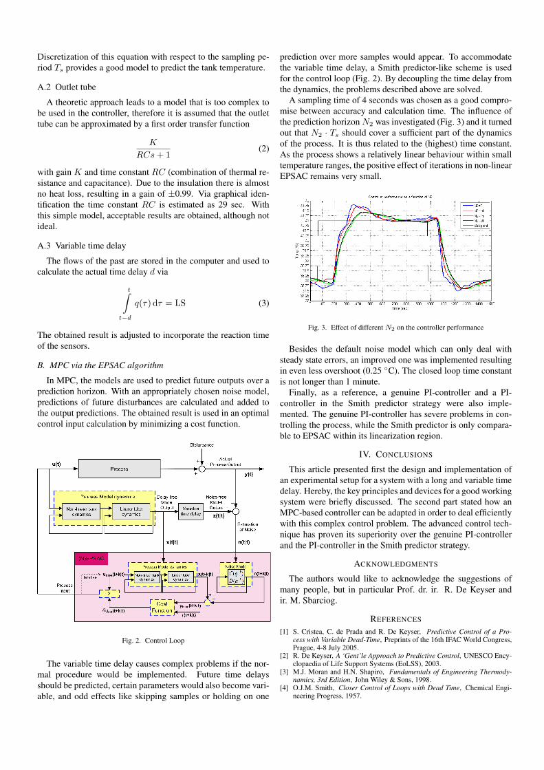
B. MPC via the EPSAC algorithm
In MPC, the models are used to predict future outputs over aprediction horizon. With an appropriately chosen noise model,predictions of future disturbances are calculated and added tothe output predictions. The obtained result is used in an optimalcontrol input calculation by minimizing a cost function.
Fig. 2. Control Loop
The variable time delay causes complex problems if the nor-mal procedure would be implemented. Future time delaysshould be predicted, certain parameters would also become vari-able, and odd effects like skipping samples or holding on one
prediction over more samples would appear. To accommodatethe variable time delay, a Smith predictor-like scheme is usedfor the control loop (Fig. 2). By decoupling the time delay fromthe dynamics, the problems described above are solved.
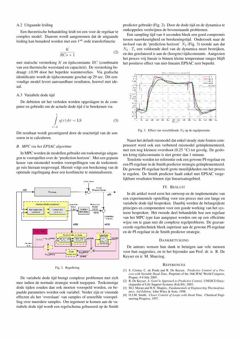
A sampling time of 4 seconds was chosen as a good compro-mise between accuracy and calculation time. The influence ofthe prediction horizon N2 was investigated (Fig. 3) and it turnedout that N2 · Ts should cover a sufficient part of the dynamicsof the process. It is thus related to the (highest) time constant.As the process shows a relatively linear behaviour within smalltemperature ranges, the positive effect of iterations in non-linearEPSAC remains very small.
Fig. 3. Effect of different N2 on the controller performance
Besides the default noise model which can only deal withsteady state errors, an improved one was implemented resultingin even less overshoot (0.25 C). The closed loop time constantis not longer than 1 minute.
Finally, as a reference, a genuine PI-controller and a PI-controller in the Smith predictor strategy were also imple-mented. The genuine PI-controller has severe problems in con-trolling the process, while the Smith predictor is only compara-ble to EPSAC within its linearization region.
IV. CONCLUSIONS
This article presented first the design and implementation ofan experimental setup for a system with a long and variable timedelay. Hereby, the key principles and devices for a good workingsystem were briefly discussed. The second part stated how anMPC-based controller can be adapted in order to deal efficientlywith this complex control problem. The advanced control tech-nique has proven its superiority over the genuine PI-controllerand the PI-controller in the Smith predictor strategy.
ACKNOWLEDGMENTS
The authors would like to acknowledge the suggestions ofmany people, but in particular Prof. dr. ir. R. De Keyser andir. M. Sbarciog.
REFERENCES
[1] S. Cristea, C. de Prada and R. De Keyser, Predictive Control of a Pro-cess with Variable Dead-Time, Preprints of the 16th IFAC World Congress,Prague, 4-8 July 2005.
[2] R. De Keyser, A ‘Gent’le Approach to Predictive Control, UNESCO Ency-clopaedia of Life Support Systems (EoLSS), 2003.
[3] M.J. Moran and H.N. Shapiro, Fundamentals of Engineering Thermody-namics, 3rd Edition, John Wiley & Sons, 1998.
[4] O.J.M. Smith, Closer Control of Loops with Dead Time, Chemical Engi-neering Progress, 1957.
Ontwerp en Geavanceerde Regelingvan een Proces met Variable Dode Tijd
Steven Himpe, Vincent Theunynck
Supervisor(s): Prof. dr. ir. R. De Keyser
Abstract—Dit artikel behandelt enerzijds het ontwerp en de implemen-tatie van een testopstelling voor een proces met variabele dode tijd, en an-derzijds een geavanceerde regelstrategie ervoor, gebruik makend van een‘Model Predictive Control’ (MPC) methode ontwikkeld aan de UniversiteitGent: EPSAC (Extended Prediction Self-Adaptive Control).
Keywords—variabele dode tijd, MPC, EPSAC, Smith predictor
I. INLEIDING
PROCESSEN met een variabele dode tijd vormen een groteuitdaging in de regeltechniek. Een dode tijd van dezelf-
de grootteorde als de tijdsconstante van het systeem, gecombi-neerd met een variatie ervan, vergen een inventieve regelstrate-gie om te voldoen aan bepaalde performantie-eisen. Gezien devele praktische toepassingen in de industrie (walsprocessen ofpapierproductie bvb.) zou het interessant zijn om een experi-mentele opstelling met variabele dode tijd te bouwen om regel-strategieen op te testen en te ontwikkelen.
De opstelling bestaat uit een watertank waarvan de tempe-ratuur moet geregeld worden. In de tank bevindt zich een ver-warmer die zorgt voor een constante warmtetoevoer (deze wordtdus niet gemanipuleerd), waardoor het water wordt opgewarmd.Een zekere temperatuur kan worden bereikt door het warme wa-ter te laten wegstromen, en evenveel koud leidingwater te latenbinnenstromen. Op deze manier blijft het watervolume in detank constant (Fig. 1). De variabele dode tijd wordt verkregendoor de temperatuursensor niet in de tank, maar in de uitgaandeleiding op zekere afstand van de tank te plaatsen. Aangezien hetdebiet varieert, is de tijd die het water nodig heeft om naar desensor te stromen eveneens variabel.
Fig. 1. Proces met variable dode tijd: een verwarmingstank
Na de implementatie van deze opstelling wordt een regelaarvan het MPC-type geprogrammeerd, met aanpassingen om tege-moet te komen aan de variabele dode tijd. Daarbij zullen ook deeffecten van de regelparameters op de prestatie van het systeemonderzocht worden.
II. ONTWERP EN IMPLEMENTATIE VAN DE OPSTELLING
A. Vereisten voor de opstelling
De dode tijd van het proces moet van dezelfde grootteordezijn als de tijdsconstante. De gesloten kring tijdsconstante moetklein zijn (≈ 1 min) en een ingangsverandering moet resulterenin een voldoende uitgangsverandering. Deze vereisten limite-ren de keuze range van de betrokken parameters (tankvol. V ,warmtetoevoer Qh, leidingvol. LS, max. debiet qmax).
Een mechanische niveauregelaar bleek de beste uitkomst vooreen constant watervolume. Na keuze van de componenten (ni-veauregelaar, 1100 W verwarmer en mixer) werd een minimuminbouwvolume van 1.13 l gehaald voor de plexiglazen tank. Deuitgaande leiding (lengte 9.5 m, vol. 1.02 l) is geısoleerd omwarmteverliezen te reduceren. Met een maximaal debiet van 2l/min wordt een temperatuur range van ±25-45 C gehaald.
B. Implementatie
De beste manier om het debiet te manipuleren is via een pe-ristaltische pomp. Met deze actieve actuator kan het debiet be-rekend worden uit de rotatiesnelheid. Een pomp met DC-motoris het makkelijkst om de snelheid te regelen: de motordrive isvoorzien van IxR compensatie om benaderend een lineair ver-band te verkrijgen tussen regelspanning en motorsnelheid (endus debiet). Naast de pomp en drive zijn ook DC spannings-bronnen nodig voor de pomp en de meetcircuits. De meetdataworden ingelezen met een geschikt DAQ-bord.
C. Temperatuurmeting
De temperatuur wordt gemeten op drie plaatsen: in de in-gaande leiding, in de tank, en op het eind van de uitgaande lei-ding. De industrieel veelgebruikte Pt100 dient als sensor. Eenwheatstone bridge met versterker zet de temperatuursafhankelij-ke weerstand om in een 0-10 V range. Passieve RC filters ver-wijderen de ruis op de signalen. Een extra digitaal filter wordtin de pc geımplementeerd. Een calibratie van de temperatuur-meting resulteert in een maximale fout van 0.4C voor de uit-laattemperatuur, en 0.8C voor de inlaattemperatuur.
III. GEAVANCEERDE REGELING
A. Modellering en identificatie
A.1 Watertank
Een energiebalans resulteert in een niet-lineaire eerste ordedifferentiaalvergelijking voor de temperatuurdynamica:
VdT (t)
dt=
Qh
ρ cp+ q(t) (Tin(t)− T (t)) (1)
Discretisering van deze vergelijking met sampling periode Ts
leidt tot een goed model om de tanktemperatuur te voorspellen.
A.2 Uitgaande leiding
Een theoretische behandeling leidt tot een voor de regelaar tecomplex model. Daarom wordt aangenomen dat de uitgaandeleiding kan benaderd worden met een 1ste orde transferfunctie
K
RCs + 1(2)
met statische versterking K en tijdsconstante RC (combinatievan een thermische weerstand en capaciteit). De versterking be-draagt ±0.99 door het beperkte warmteverlies. Via grafischeidentificatie wordt de tijdsconstante geschat op 29 sec. Dit een-voudige model levert aanvaardbare resultaten, hoewel niet ide-aal.
A.3 Variabele dode tijd
De debieten uit het verleden worden opgeslagen in de com-puter en gebruikt om de actuele dode tijd d te berekenen via
t∫t−d
q(τ) dτ = LS (3)
Dit resultaat wordt gecorrigeerd door de reactietijd van de sen-soren in te calculeren.
B. MPC via het EPSAC algoritme
In MPC worden de modellen gebruikt om toekomstige uitgan-gen te voorspellen over de ‘prediction horizon’. Met een gepastekeuze van ruismodel worden voorspellingen van de toekomsti-ge ruis hieraan toegevoegd. Hieruit volgt een berekening van deoptimale regelingang door een kostfunctie te minimaliseren.
Fig. 2. Regelkring
De variabele dode tijd brengt complexe problemen met zichmee indien de normale strategie wordt toegepast. Toekomstigedode tijden zouden dan ook moeten voorspeld worden, en be-paalde parameters worden ook variabel. Verder zijn er vreemdeeffecten als het ‘overslaan’ van samples of eenzelfde voorspel-ling over meerdere samples. Om tegemoet te komen aan de va-riabele dode tijd wordt een regelschema gebaseerd op de Smith
predictor gebruikt (Fig. 2). Door de dode tijd en de dynamica teontkoppelen verdwijnen de bovenstaande problemen.
Een sampling tijd van 4 seconden bleek een goed compromistussen nauwkeurigheid en berekeningstijd. Onderzoek naar deinvloed van de ‘prediction horizon’ N2 (Fig. 3) toonde aan datN2 · Ts een voldoende deel van de dynamica moet bestrijken,en dus gerelateerd is aan de (hoogste) tijdsconstante. Aangezienhet proces vrij lineair is binnen kleine temperatuur ranges blijfthet positieve effect van niet-lineaire EPSAC zeer beperkt.
Fig. 3. Effect van verschillende N2 op de regelprestatie
Naast het default ruismodel dat enkel steady state fouten com-penseert werd ook een verbeterd ruismodel geımplementeerd,met een nog kleinere overshoot (0.25 C) tot gevolg. De geslo-ten kring tijdsconstante is niet groter dan 1 minuut.
Tenslotte werden ter referentie ook een gewone PI-regelaar eneen PI-regelaar in de Smith predictor strategie geımplementeerd.De gewone PI-regelaar heeft grote moeilijkheden om het proceste regelen. De Smith predictor haalt enkel met EPSAC verge-lijkbare resultaten binnen zijn linearisatiegebied.
IV. BESLUIT
In dit artikel werd eerst het ontwerp en de implementatie vaneen experimentele opstelling voor een proces met een lange envariabele dode tijd besproken. Daarbij werden de belangrijksteprincipes en componenten voor een goede werking van het sys-teem besproken. Het tweede deel behandelde hoe een regelaarvan het MPC type kan aangepast worden om op een efficientewijze om te gaan met dit complexe regelprobleem. De geavan-ceerde regeltechniek bleek superieur aan de gewone PI-regelaaren de PI-regelaar in de Smith predictor strategie.
DANKBETUIGING
De auteurs wensen hun dank te betuigen aan vele mensenvoor hun suggesties, en in het bijzonder aan Prof. dr. ir. R. DeKeyser en ir. M. Sbarciog.
REFERENCES
[1] S. Cristea, C. de Prada and R. De Keyser, Predictive Control of a Pro-cess with Variable Dead-Time, Preprints of the 16th IFAC World Congress,Prague, 4-8 July 2005.
[2] R. De Keyser, A ‘Gent’le Approach to Predictive Control, UNESCO Ency-clopaedia of Life Support Systems (EoLSS), 2003.
[3] M.J. Moran and H.N. Shapiro, Fundamentals of Engineering Thermodyna-mics, 3rd Edition, John Wiley & Sons, 1998.
[4] O.J.M. Smith, Closer Control of Loops with Dead Time, Chemical Engi-neering Progress, 1957.
Contents
Preface ii
Survey iii
Extended abstract iv
1 Introduction 1
I Design and Implementation 7
2 Requirements for the setup 82.1 Choice of parameters . . . . . . . . . . . . . . . . . . . . . . . . . . . . . . . . 8
2.1.1 Crucial design parameters . . . . . . . . . . . . . . . . . . . . . . . . . 82.1.2 Functional relations . . . . . . . . . . . . . . . . . . . . . . . . . . . . 92.1.3 Conclusion . . . . . . . . . . . . . . . . . . . . . . . . . . . . . . . . . 10
2.2 Design types for constant water volume . . . . . . . . . . . . . . . . . . . . . 122.2.1 Preliminaries . . . . . . . . . . . . . . . . . . . . . . . . . . . . . . . . 122.2.2 The pressurized tank . . . . . . . . . . . . . . . . . . . . . . . . . . . . 132.2.3 The communicating vessels . . . . . . . . . . . . . . . . . . . . . . . . 142.2.4 The relay-guarded level . . . . . . . . . . . . . . . . . . . . . . . . . . 142.2.5 The float switch-guarded level . . . . . . . . . . . . . . . . . . . . . . . 152.2.6 Conclusion . . . . . . . . . . . . . . . . . . . . . . . . . . . . . . . . . 16
2.3 Communicating Vessels . . . . . . . . . . . . . . . . . . . . . . . . . . . . . . 162.3.1 Theoretical approach . . . . . . . . . . . . . . . . . . . . . . . . . . . . 172.3.2 Results . . . . . . . . . . . . . . . . . . . . . . . . . . . . . . . . . . . 222.3.3 Conclusion . . . . . . . . . . . . . . . . . . . . . . . . . . . . . . . . . 23
2.4 Float switch-guarded level . . . . . . . . . . . . . . . . . . . . . . . . . . . . . 232.4.1 Theoretical approach . . . . . . . . . . . . . . . . . . . . . . . . . . . . 232.4.2 Conclusion . . . . . . . . . . . . . . . . . . . . . . . . . . . . . . . . . 27
3 Mechanical and electrical implementation 283.1 Flow Control . . . . . . . . . . . . . . . . . . . . . . . . . . . . . . . . . . . . 28
3.1.1 Types of actuators . . . . . . . . . . . . . . . . . . . . . . . . . . . . . 28
ix
CONTENTS x
3.1.2 Controlling the flow . . . . . . . . . . . . . . . . . . . . . . . . . . . . 293.2 DC-sources for the temperature measurement . . . . . . . . . . . . . . . . . . 313.3 Data acquisition . . . . . . . . . . . . . . . . . . . . . . . . . . . . . . . . . . 32
3.3.1 Requirements . . . . . . . . . . . . . . . . . . . . . . . . . . . . . . . . 323.3.2 Selection . . . . . . . . . . . . . . . . . . . . . . . . . . . . . . . . . . 33
3.4 Overview . . . . . . . . . . . . . . . . . . . . . . . . . . . . . . . . . . . . . . 343.4.1 Process tank . . . . . . . . . . . . . . . . . . . . . . . . . . . . . . . . 343.4.2 Electrical supply . . . . . . . . . . . . . . . . . . . . . . . . . . . . . . 353.4.3 Water circuit . . . . . . . . . . . . . . . . . . . . . . . . . . . . . . . . 37
4 Temperature Measurement 404.1 Choice of the sensor . . . . . . . . . . . . . . . . . . . . . . . . . . . . . . . . 40
4.1.1 Different types of sensors . . . . . . . . . . . . . . . . . . . . . . . . . 404.1.2 The Pt100 sensor . . . . . . . . . . . . . . . . . . . . . . . . . . . . . . 43
4.2 Measurement circuits . . . . . . . . . . . . . . . . . . . . . . . . . . . . . . . . 444.2.1 Preliminaries . . . . . . . . . . . . . . . . . . . . . . . . . . . . . . . . 444.2.2 Excitation via a fixed current source . . . . . . . . . . . . . . . . . . . 444.2.3 Excitation via the Wheatstone bridge . . . . . . . . . . . . . . . . . . 454.2.4 The differential amplifier circuit . . . . . . . . . . . . . . . . . . . . . 474.2.5 The instrumentation amplifier circuit . . . . . . . . . . . . . . . . . . . 494.2.6 Conclusions . . . . . . . . . . . . . . . . . . . . . . . . . . . . . . . . . 49
4.3 Noise analysis and filtering . . . . . . . . . . . . . . . . . . . . . . . . . . . . 514.4 Calibration . . . . . . . . . . . . . . . . . . . . . . . . . . . . . . . . . . . . . 55
II Advanced Control 59
5 Modelling and Identification 605.1 Preliminaries . . . . . . . . . . . . . . . . . . . . . . . . . . . . . . . . . . . . 605.2 Water tank . . . . . . . . . . . . . . . . . . . . . . . . . . . . . . . . . . . . . 605.3 Heat loss . . . . . . . . . . . . . . . . . . . . . . . . . . . . . . . . . . . . . . 62
5.3.1 Of the tank . . . . . . . . . . . . . . . . . . . . . . . . . . . . . . . . . 625.3.2 In the tube . . . . . . . . . . . . . . . . . . . . . . . . . . . . . . . . . 64
5.4 Outlet Tube . . . . . . . . . . . . . . . . . . . . . . . . . . . . . . . . . . . . . 675.4.1 Dynamics . . . . . . . . . . . . . . . . . . . . . . . . . . . . . . . . . . 675.4.2 Variable Time Delay . . . . . . . . . . . . . . . . . . . . . . . . . . . . 69
5.5 Identification . . . . . . . . . . . . . . . . . . . . . . . . . . . . . . . . . . . . 715.5.1 Water Tank . . . . . . . . . . . . . . . . . . . . . . . . . . . . . . . . . 725.5.2 Outlet Tube . . . . . . . . . . . . . . . . . . . . . . . . . . . . . . . . . 755.5.3 Variable Time Delay . . . . . . . . . . . . . . . . . . . . . . . . . . . . 76
CONTENTS xi
6 Controllers 786.1 Non-linear EPSAC controller . . . . . . . . . . . . . . . . . . . . . . . . . . . 79
6.1.1 General approach . . . . . . . . . . . . . . . . . . . . . . . . . . . . . . 796.1.2 Control loop layout . . . . . . . . . . . . . . . . . . . . . . . . . . . . . 816.1.3 Choice of Ts . . . . . . . . . . . . . . . . . . . . . . . . . . . . . . . . . 896.1.4 Influence of N2 . . . . . . . . . . . . . . . . . . . . . . . . . . . . . . . 896.1.5 Influence of Ni . . . . . . . . . . . . . . . . . . . . . . . . . . . . . . . 916.1.6 Noise model . . . . . . . . . . . . . . . . . . . . . . . . . . . . . . . . . 96
6.2 Genuine PI-controller and Smith predictor . . . . . . . . . . . . . . . . . . . . 996.2.1 PI-controller . . . . . . . . . . . . . . . . . . . . . . . . . . . . . . . . 1006.2.2 PI-controller in the Smith predictor strategy . . . . . . . . . . . . . . 103
7 Conclusions 1087.1 The setup . . . . . . . . . . . . . . . . . . . . . . . . . . . . . . . . . . . . . . 1087.2 Advanced Control . . . . . . . . . . . . . . . . . . . . . . . . . . . . . . . . . 109
A GUIDE 112A.1 Introduction and Installation . . . . . . . . . . . . . . . . . . . . . . . . . . . 112A.2 Control structure . . . . . . . . . . . . . . . . . . . . . . . . . . . . . . . . . . 112A.3 Interfaces . . . . . . . . . . . . . . . . . . . . . . . . . . . . . . . . . . . . . . 113A.4 Precautions . . . . . . . . . . . . . . . . . . . . . . . . . . . . . . . . . . . . . 118
List of Figures 120
Bibliography 123
Chapter 1
Introduction
In control engineering, systems with time delay have always required extra effort to design anadequate controller. A delayed reaction to the applied inputs might cause a control outputwhich is too fierce, resulting in a high overshoot after the time delay has passed. The bestexample one could give to illustrate the difficulties in controlling such processes comes fromevery-day life: a person who wants to take a shower. The person will manipulate the hotwater tap in his attempt to reach the optimal temperature; however the effects of his controlactions will only be experienced after the water has flowed through the water tube (transportdelay), and touches his skin, which acts as a sensor. The person, who obviously wants toreach the optimal temperature as soon as possible, will therefore be inclined to turn the valvetoo fiercely, with too cold or too hot water as a result.
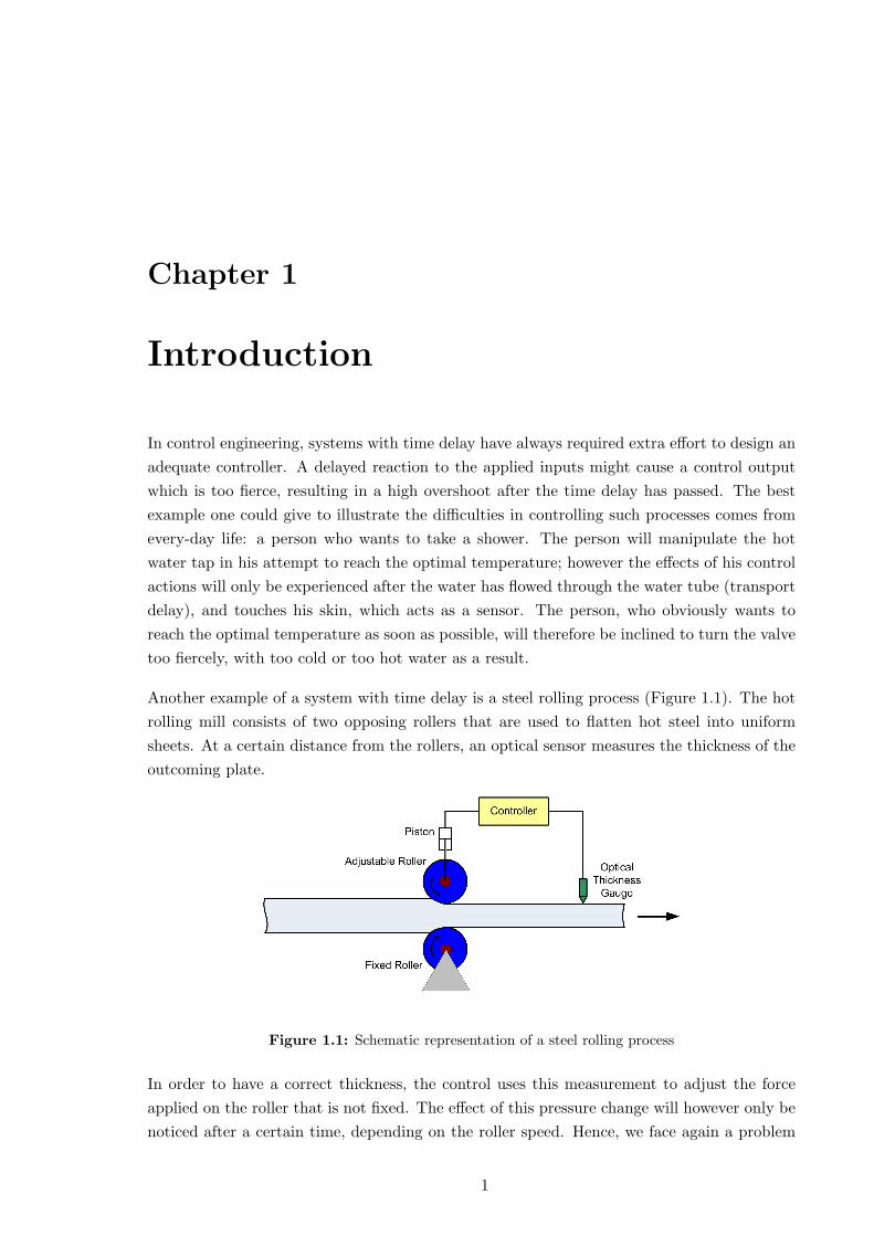
Another example of a system with time delay is a steel rolling process (Figure 1.1). The hotrolling mill consists of two opposing rollers that are used to flatten hot steel into uniformsheets. At a certain distance from the rollers, an optical sensor measures the thickness of theoutcoming plate.
Figure 1.1: Schematic representation of a steel rolling process
In order to have a correct thickness, the control uses this measurement to adjust the forceapplied on the roller that is not fixed. The effect of this pressure change will however only benoticed after a certain time, depending on the roller speed. Hence, we face again a problem
1
CHAPTER 1. INTRODUCTION 2
with time delay. Considering the high quality requirements of steel plates, there is a lot togain from an adequate control.
A last example is that of pharmacokinetics, a discipline in which the time course of the drugconcentration throughout the body, and its relation to the organism or system, is investigatedand modelled. When medicine is administered to a patient, it takes a certain time before anorgan experiences the influence of the drug, while that might be faster or slower for anotherorgan. It is obvious that the time delay is an extremely important factor here, for examplein the case of anaesthesia, where an error can have life-threatening consequences. Moreover,it is an extremely difficult parameter to model, since it might change from person to person,from organ to organ, and even be dependent on the moment.
Trends in controlling systems with time delay
Problems with time delay require in a sense a certain form of patience and/or knowledgeof the process. During years, many solutions have been postulated to achieve good controlperformances, amongst which the most important ones are:
• ‘De-tuning’ of a PID-controller:In this strategy the sensitivity of the PID-controller is being diminished. This is donemainly by reducing the integrator-action: the integrator is responsible for a continuousincrease of the controller output as long as there is a difference between setpoint andprocess output. This result is reinforced by the slow response due to the time delay. By‘de-tuning’, this influence is reduced, with a positive effect on the controlled process. Ina famous paper from 1942 [24], Ziegler and Nichols suggested that the best option is toreduce the integration constant by a factor of 1/d2, where d represents the time delayof the process. The proportional action should be reduced with a factor 1/d, while thedifferential action should not be changed.
• Smith predictor:In the Smith predictor control strategy [17] - proposed by Otto Smith in 1957 - thecontroller is provided with ‘foreknowledge’ of the time delay. First, one tries to developa mathematical model of the process, in which the dynamics are decoupled from thetime delay (Figure 1.2). Then the output of the model (with time delay) is compared tothe real process output in order to have an estimation of the noise. This noise is addedto the output of the model without time delay, the result is fed back and comparedto the actual setpoint. The error is then supplied to a simple controller (a PID forinstance), tuned as if there was no time delay at all.
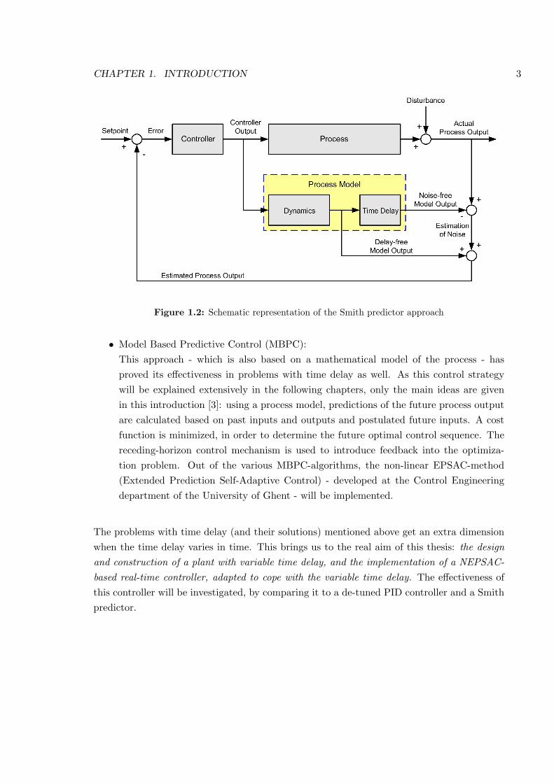
CHAPTER 1. INTRODUCTION 3
Figure 1.2: Schematic representation of the Smith predictor approach
• Model Based Predictive Control (MBPC):This approach - which is also based on a mathematical model of the process - hasproved its effectiveness in problems with time delay as well. As this control strategywill be explained extensively in the following chapters, only the main ideas are givenin this introduction [3]: using a process model, predictions of the future process outputare calculated based on past inputs and outputs and postulated future inputs. A costfunction is minimized, in order to determine the future optimal control sequence. Thereceding-horizon control mechanism is used to introduce feedback into the optimiza-tion problem. Out of the various MBPC-algorithms, the non-linear EPSAC-method(Extended Prediction Self-Adaptive Control) - developed at the Control Engineeringdepartment of the University of Ghent - will be implemented.
The problems with time delay (and their solutions) mentioned above get an extra dimensionwhen the time delay varies in time. This brings us to the real aim of this thesis: the designand construction of a plant with variable time delay, and the implementation of a NEPSAC-based real-time controller, adapted to cope with the variable time delay. The effectiveness ofthis controller will be investigated, by comparing it to a de-tuned PID controller and a Smithpredictor.
CHAPTER 1. INTRODUCTION 4
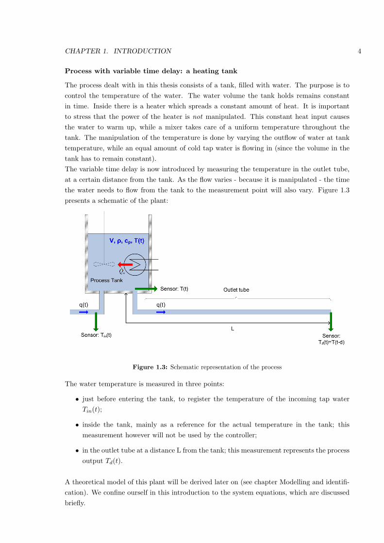
Process with variable time delay: a heating tank
The process dealt with in this thesis consists of a tank, filled with water. The purpose is tocontrol the temperature of the water. The water volume the tank holds remains constantin time. Inside there is a heater which spreads a constant amount of heat. It is importantto stress that the power of the heater is not manipulated. This constant heat input causesthe water to warm up, while a mixer takes care of a uniform temperature throughout thetank. The manipulation of the temperature is done by varying the outflow of water at tanktemperature, while an equal amount of cold tap water is flowing in (since the volume in thetank has to remain constant).The variable time delay is now introduced by measuring the temperature in the outlet tube,at a certain distance from the tank. As the flow varies - because it is manipulated - the timethe water needs to flow from the tank to the measurement point will also vary. Figure 1.3presents a schematic of the plant:
Figure 1.3: Schematic representation of the process
The water temperature is measured in three points:
• just before entering the tank, to register the temperature of the incoming tap waterTin(t);
• inside the tank, mainly as a reference for the actual temperature in the tank; thismeasurement however will not be used by the controller;
• in the outlet tube at a distance L from the tank; this measurement represents the processoutput Td(t).
A theoretical model of this plant will be derived later on (see chapter Modelling and identifi-cation). We confine ourself in this introduction to the system equations, which are discussedbriefly.
CHAPTER 1. INTRODUCTION 5
The temperature dynamics of the water in the tank satisfy the following non-linear first orderdifferential equation, which is obtained by applying an energy balance on the system:
VdT (t)
dt=
Qh
ρ cp+ q(t) (Tin(t)− T (t)) (1.1)
where
• V : the volume of water in the tank;
• T (t): the temperature of the water in the tank;
• Qh: the amount of heat coming from the heater (constant);
• ρ: the density of water;
• cp: the specific heat coefficient of water;
• q(t): the flow which enters/leaves the tank;
• Tin(t): the temperature of the incoming tap water.
The time constant of this process is defined as:
τ =V
q(t)(1.2)
By measuring the temperature in the outlet tube with length L and section S, a time delayd is introduced, hence the temperature at the measurement point (assuming no heat loss andno dynamics in the tube) can be written as:
Td(t) = T (t− d) (1.3)
where the variable time delay depends on the flows applied to the process. If the flow doesnot change (q(t)=constant), this time delay is given by:
d =LS
q(t)(1.4)
In order to increase the complexity of the process, which makes it more challenging from thecontrol point of view, the outlet tube should be designed in such a way that the time delayis approximately equal to the time constant of the process.
CHAPTER 1. INTRODUCTION 6
Content and structure of the thesis
Several subjects will be treated in this thesis. Roughly, the structure can be divided into twomain parts: first the Design and implementation of the entire setup, and second the Advancedcontrol of the process.
The first topic in Design and implementation handles the Requirements for the setup (Chap-ter 2). This chapter introduces conditions the design should fulfill as well as possible imple-mentation solutions. Functional relations between several important parameters are derived,where the parameters are chosen in such a way that the controlled temperature range ismaximized and setpoint changes within that region can be reached in a short time. Severaldesigns will be investigated and tested against feasibility, cost and effectiveness.
Next, the Mechanical and electrical implementation (Chapter 3) of the plant is discussed. Afirst section handles the way the flow is manipulated, discussing the type of actuators thatare needed and methods to efficiently control them. Further on, a brief word will be spent onthe measurements and the data acquisition. In the end, an overview of the whole setup willbe given.
As it is a crucial part for the success of the control, a separate chapter deals with the Tem-perature measurement (Chapter 4), discussing the type of sensors and requirements for themeasurement, the circuitry to convert it to a useful signal and the calibration of the circuits.
With the design and implementation of the plant done, we arrive at the part handling theAdvanced Control. In Modelling and identification (Chapter 5) theoretical models of the watertank, the heat loss, and the outlet tube will be derived. Afterwards the results will be testedagainst experimental data, to tune the models in the identification section.
Having obtained reliable models, Controllers (Chapter 6) can be designed in order to improvethe performance compared to the open loop response. In the first section the NEPSAC-algorithm will be explained, with the adjustments to deal with the variable time delay. Af-terwards, measurements are performed and the influence of several parameters is examined.In order to have a point of comparison, a genuine PID-controller, and a PID-controller in theSmith predictor strategy are also implemented in the last two sections.
In the last chapter the main results will be summarized and the final Conclusions of thisthesis will be drawn (Chapter 7).
Appendix A contains a GUIDE for the Graphical User Interface that is programmed tomanage the different controllers and perform experiments in an easy way. Instructions forthe correct use of the setup are also given.
Part I
Design and Implementation
7
Chapter 2
Requirements for the setup
2.1 Choice of parameters
2.1.1 Crucial design parameters
When the idea of the heating tank system was presented, three important demands were tobe satisfied:
1. A unit change in the input produces a significant change in the output.
2. The closed loop time constant equals roughly one minute.
3. The time constant of the tank is more or less equal to the transport delay1.
V
q≈ L
qS
(2.1)
The first two demands both require the process to be ‘sufficiently sensitive’. This means achange in the flow - which is the controlled variable - should result quite rapidly in a changeof the temperature. The third demand relates the volume of the tank to the volume of theoutlet tube: both volumes have to be approximately equal.
Intuitively, it is clear that only few parameters are determinant for the process dynamics.For instance, a high power heater will heat the water in the tank very fast, while applyinglarge flows to the process will cause a large temperature drop. The volume of the tank isalso important: taking it too large will result in modest changes in temperature. Hence thechoice of parameters Qh (the heat input), qmax (the maximum flow) and V (the controlledwater volume) influences the sensitivity of the process and, consequently, determines whetheror not the first two design requirements are met. Under these considerations, it is obviousthat for a good design a more detailed mathematical analysis is necessary.
1This equation assumes constant flow q. L denotes the length of the outlet tube while qS
is the velocity of
the outflow.
8
CHAPTER 2. REQUIREMENTS FOR THE SETUP 9
2.1.2 Functional relations
To derive functional relations between parameters Qh, qmax and V , we start from the equationdescribing the process dynamics:
VdT (t)
dt=
Qh
ρcp+ q(t)(Tin(t)− T (t)) (2.2)
As the flow q(t) will be the manipulated variable in our control problem, the sensitivity of theprocess must be interpreted as the net effect a change in the flow has on the tank temperature.Subsequently, the relationship between q(t) and
∣∣∣dT (t)dt
∣∣∣ has to be examined more closely.Assuming a tank temperature Tc - where c denotes the current operating point - the maximumtemperature drop is reached when applying the maximum flow (the incoming temperatureTin is considered to remain constant):(
dT (t)dt
)min
=Qh
ρcpV+
qmax
V(Tin − Tc) (2.3)
while zero flow accounts for maximum temperature increase:(dT (t)
dt
)max
=Qh
ρcpV(2.4)
By defining a coefficient ξ, the maximum cooling rate (2.3) can be related to the maximumheating rate (2.4) at the current operating point:
ξ = −
(dT (t)
dt
)min(
dT (t)dt
)max
= −Qh
ρcpV + qmax
V (Tin − Tc)Qh
ρcpV
(2.5)
This allows to determine an operating range of temperatures Tc - given by ξ ≈ 1 - wherewarming up or cooling down take about the same time. Consequently, temperatures withinthis range - above or below the current operating point Tc - can be reached in limited time.This is important considering the limited closed loop time constant. Simplifying (2.5) a linearrelation between ξ and Tc appears:
Tc =Qh
ρcpqmax(1 + ξ) + Tin (2.6)
The central operating point is defined as the temperature at which maximum cooling rate (2.3)and maximum heating rate (2.4) have equal absolute values, expressed by ξ = 1. It corre-sponds to the steady state temperature Tcc:
Tcc = Tin +Qh
ρcpqmax
2
(2.7)
Thus, the heating power Qh and the maximum flow qmax both determine the position ofthe central operating point and the slope of the linear characteristic describing the operatingrange. It is interesting from the control point of view to maximize this range. On one hand,this means maximizing the slope of the linear characteristic, while on the other hand the
CHAPTER 2. REQUIREMENTS FOR THE SETUP 10
central operating point must be lowered to reduce ambient heat loss. The choice of qmax
comes with yet another requirement, that of the minimum time delay.
dmin =L
qmax
S
(2.8)
It is clear that a small maximum flow will result in huge time delays. However, these time de-lays have to be limited taking into account the second requirement (closed loop time constantof approximately one minute). As a result, a restriction for qmax applies:
LS
1 min<< qmax (2.9)
This formula, together with formulas (2.1), (2.6) and (2.7) provides functional relations be-tween the process’s crucial parameters: the choice of the heat input Qh appears to be depen-dent on the choice of qmax, which is in turn related to the volume of the outlet tube LS andtherefore dependent on the volume of the tank V .
2.1.3 Conclusion
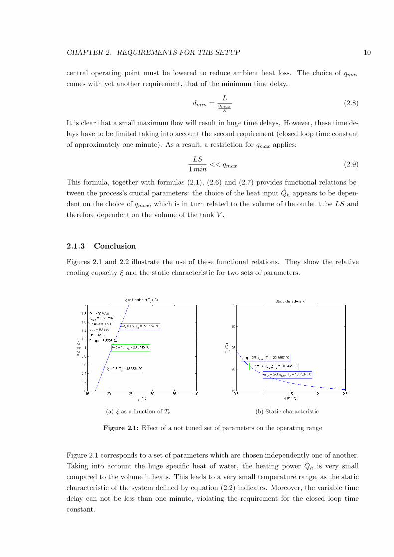
Figures 2.1 and 2.2 illustrate the use of these functional relations. They show the relativecooling capacity ξ and the static characteristic for two sets of parameters.
(a) ξ as a function of Tc (b) Static characteristic
Figure 2.1: Effect of a not tuned set of parameters on the operating range
Figure 2.1 corresponds to a set of parameters which are chosen independently one of another.Taking into account the huge specific heat of water, the heating power Qh is very smallcompared to the volume it heats. This leads to a very small temperature range, as the staticcharacteristic of the system defined by equation (2.2) indicates. Moreover, the variable timedelay can not be less than one minute, violating the requirement for the closed loop timeconstant.
CHAPTER 2. REQUIREMENTS FOR THE SETUP 11
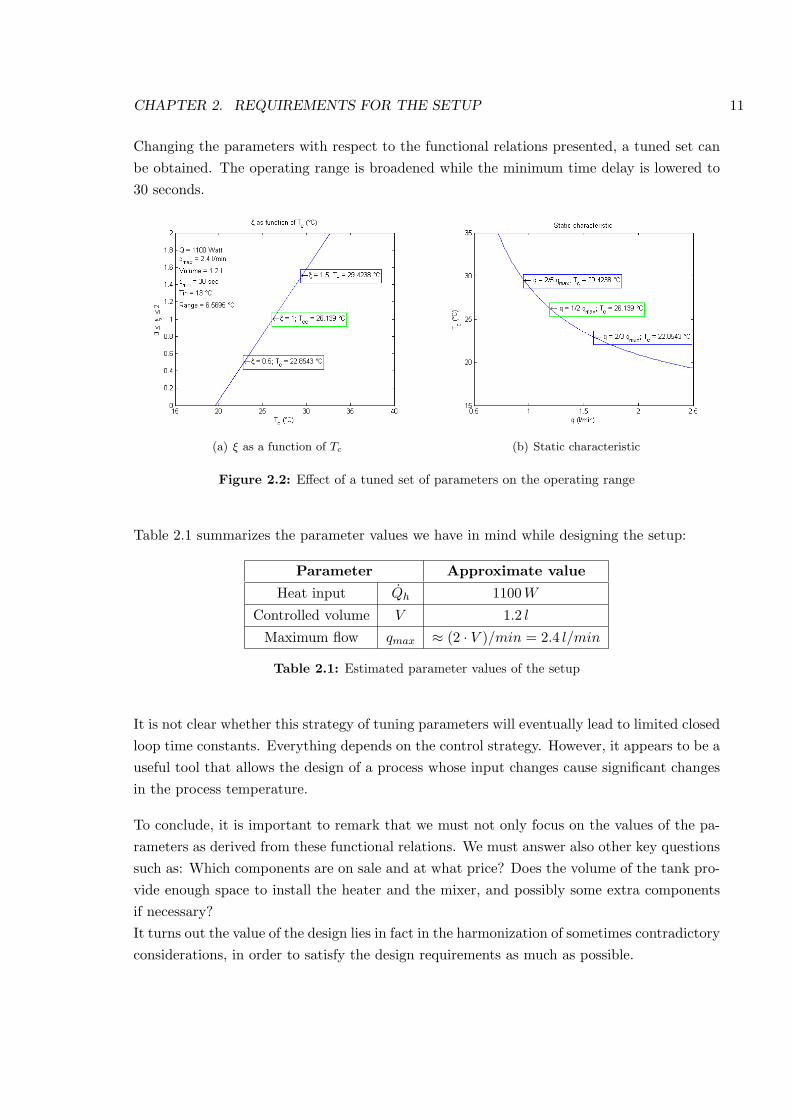
Changing the parameters with respect to the functional relations presented, a tuned set canbe obtained. The operating range is broadened while the minimum time delay is lowered to30 seconds.
(a) ξ as a function of Tc (b) Static characteristic
Figure 2.2: Effect of a tuned set of parameters on the operating range
Table 2.1 summarizes the parameter values we have in mind while designing the setup:
Parameter Approximate value
Heat input Qh 1100 W
Controlled volume V 1.2 l
Maximum flow qmax ≈ (2 · V )/min = 2.4 l/min
Table 2.1: Estimated parameter values of the setup
It is not clear whether this strategy of tuning parameters will eventually lead to limited closedloop time constants. Everything depends on the control strategy. However, it appears to be auseful tool that allows the design of a process whose input changes cause significant changesin the process temperature.
To conclude, it is important to remark that we must not only focus on the values of the pa-rameters as derived from these functional relations. We must answer also other key questionssuch as: Which components are on sale and at what price? Does the volume of the tank pro-vide enough space to install the heater and the mixer, and possibly some extra componentsif necessary?It turns out the value of the design lies in fact in the harmonization of sometimes contradictoryconsiderations, in order to satisfy the design requirements as much as possible.
CHAPTER 2. REQUIREMENTS FOR THE SETUP 12
2.2 Design types for constant water volume
2.2.1 Preliminaries
The previous section treated the design from a control point of view. Functional relationsbetween several parameters were presented in order to maximize the operating range. Froma practical point of view however, an important assumption has been made: the volume ofwater is constant, irrespective of the amount of water flowing into or out of the tank. This ofcourse strongly reduces the complexity of the process dynamics.
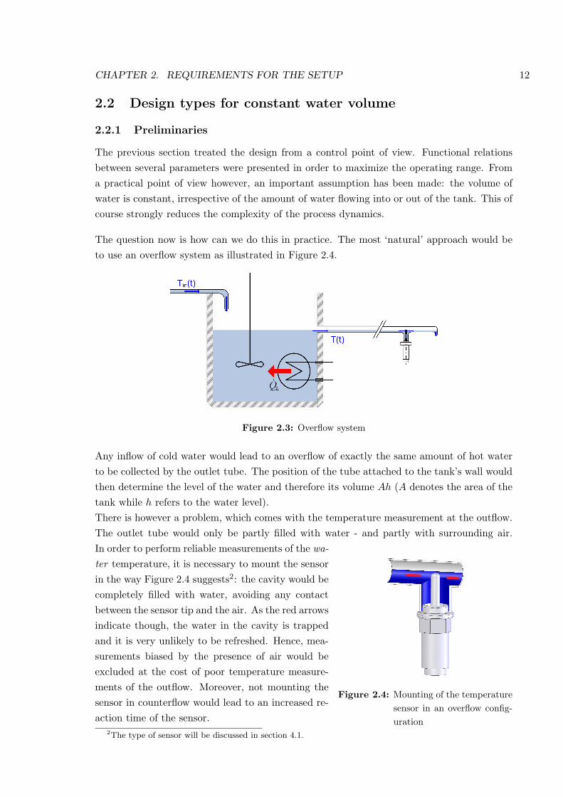
The question now is how can we do this in practice. The most ‘natural’ approach would beto use an overflow system as illustrated in Figure 2.4.
Figure 2.3: Overflow system
Any inflow of cold water would lead to an overflow of exactly the same amount of hot waterto be collected by the outlet tube. The position of the tube attached to the tank’s wall wouldthen determine the level of the water and therefore its volume Ah (A denotes the area of thetank while h refers to the water level).There is however a problem, which comes with the temperature measurement at the outflow.The outlet tube would only be partly filled with water - and partly with surrounding air.
Figure 2.4: Mounting of the temperaturesensor in an overflow config-uration
In order to perform reliable measurements of the wa-ter temperature, it is necessary to mount the sensorin the way Figure 2.4 suggests2: the cavity would becompletely filled with water, avoiding any contactbetween the sensor tip and the air. As the red arrowsindicate though, the water in the cavity is trappedand it is very unlikely to be refreshed. Hence, mea-surements biased by the presence of air would beexcluded at the cost of poor temperature measure-ments of the outflow. Moreover, not mounting thesensor in counterflow would lead to an increased re-action time of the sensor.
2The type of sensor will be discussed in section 4.1.
CHAPTER 2. REQUIREMENTS FOR THE SETUP 13
In fact, the use of an overflowing tank appears to have serious consequences regarding thetemperature measurements. Therefore, it is necessary to think of other designs which combinetwo important issues:
• The water level is constant, irrespective of the amount of cold water flowing in.
• The outlet and inlet tubes are completely filled at all times.
The following sections deal with several designs that succeed to meet both requirements. Thecost and the feasibility of every design are, of course, of great importance. The ones thateventually fulfill all demands will be treated more in depth afterwards.
2.2.2 The pressurized tank
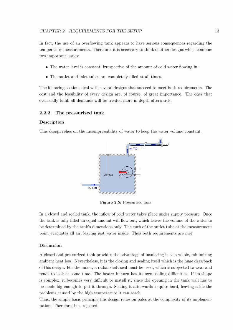
Description
This design relies on the incompressibility of water to keep the water volume constant.
Figure 2.5: Pressurized tank
In a closed and sealed tank, the inflow of cold water takes place under supply pressure. Oncethe tank is fully filled an equal amount will flow out, which leaves the volume of the water tobe determined by the tank’s dimensions only. The curb of the outlet tube at the measurementpoint evacuates all air, leaving just water inside. Thus both requirements are met.
Discussion
A closed and pressurized tank provides the advantage of insulating it as a whole, minimizingambient heat loss. Nevertheless, it is the closing and sealing itself which is the huge drawbackof this design. For the mixer, a radial shaft seal must be used, which is subjected to wear andtends to leak at some time. The heater in turn has its own sealing difficulties. If its shapeis complex, it becomes very difficult to install it, since the opening in the tank wall has tobe made big enough to put it through. Sealing it afterwards is quite hard, leaving aside theproblems caused by the high temperature it can reach.Thus, the simple basic principle this design relies on pales at the complexity of its implemen-tation. Therefore, it is rejected.
CHAPTER 2. REQUIREMENTS FOR THE SETUP 14
2.2.3 The communicating vessels
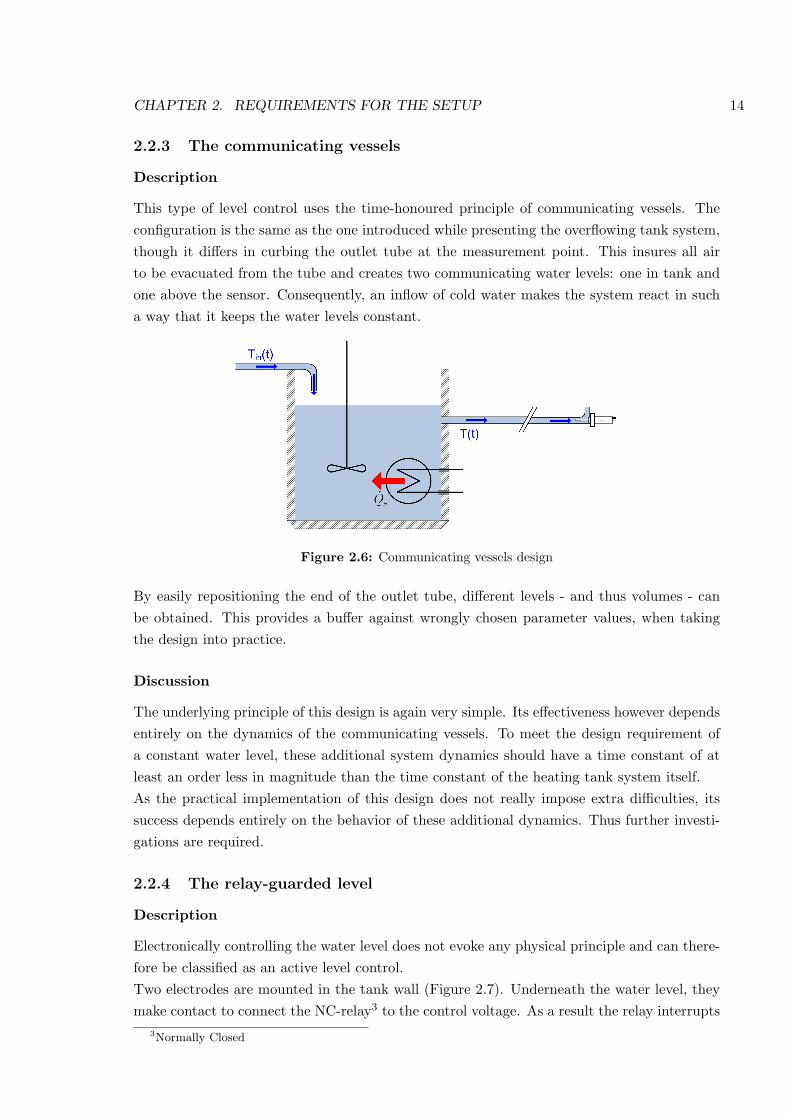
Description
This type of level control uses the time-honoured principle of communicating vessels. Theconfiguration is the same as the one introduced while presenting the overflowing tank system,though it differs in curbing the outlet tube at the measurement point. This insures all airto be evacuated from the tube and creates two communicating water levels: one in tank andone above the sensor. Consequently, an inflow of cold water makes the system react in sucha way that it keeps the water levels constant.
Figure 2.6: Communicating vessels design
By easily repositioning the end of the outlet tube, different levels - and thus volumes - canbe obtained. This provides a buffer against wrongly chosen parameter values, when takingthe design into practice.
Discussion
The underlying principle of this design is again very simple. Its effectiveness however dependsentirely on the dynamics of the communicating vessels. To meet the design requirement ofa constant water level, these additional system dynamics should have a time constant of atleast an order less in magnitude than the time constant of the heating tank system itself.As the practical implementation of this design does not really impose extra difficulties, itssuccess depends entirely on the behavior of these additional dynamics. Thus further investi-gations are required.
2.2.4 The relay-guarded level
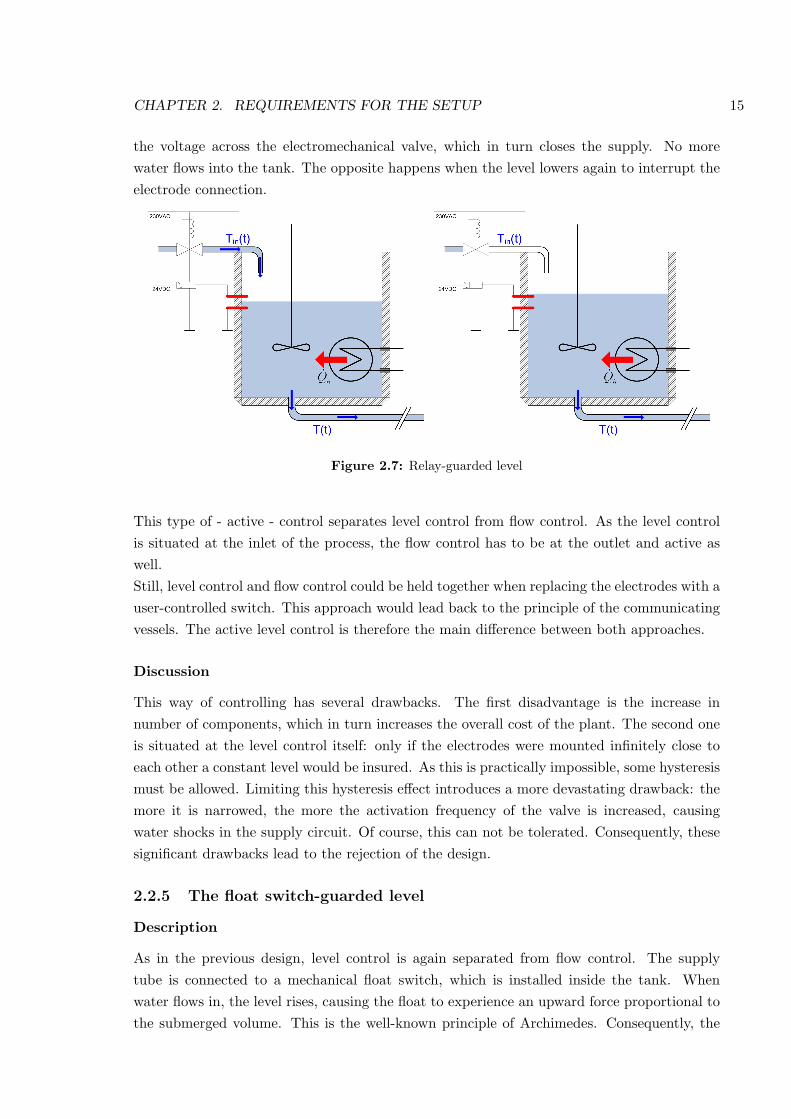
Description
Electronically controlling the water level does not evoke any physical principle and can there-fore be classified as an active level control.Two electrodes are mounted in the tank wall (Figure 2.7). Underneath the water level, theymake contact to connect the NC-relay3 to the control voltage. As a result the relay interrupts
3Normally Closed
CHAPTER 2. REQUIREMENTS FOR THE SETUP 15
the voltage across the electromechanical valve, which in turn closes the supply. No morewater flows into the tank. The opposite happens when the level lowers again to interrupt theelectrode connection.
Figure 2.7: Relay-guarded level
This type of - active - control separates level control from flow control. As the level controlis situated at the inlet of the process, the flow control has to be at the outlet and active aswell.Still, level control and flow control could be held together when replacing the electrodes with auser-controlled switch. This approach would lead back to the principle of the communicatingvessels. The active level control is therefore the main difference between both approaches.
Discussion
This way of controlling has several drawbacks. The first disadvantage is the increase innumber of components, which in turn increases the overall cost of the plant. The second oneis situated at the level control itself: only if the electrodes were mounted infinitely close toeach other a constant level would be insured. As this is practically impossible, some hysteresismust be allowed. Limiting this hysteresis effect introduces a more devastating drawback: themore it is narrowed, the more the activation frequency of the valve is increased, causingwater shocks in the supply circuit. Of course, this can not be tolerated. Consequently, thesesignificant drawbacks lead to the rejection of the design.
2.2.5 The float switch-guarded level
Description
As in the previous design, level control is again separated from flow control. The supplytube is connected to a mechanical float switch, which is installed inside the tank. Whenwater flows in, the level rises, causing the float to experience an upward force proportional tothe submerged volume. This is the well-known principle of Archimedes. Consequently, the
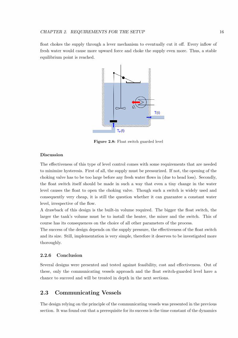
CHAPTER 2. REQUIREMENTS FOR THE SETUP 16
float chokes the supply through a lever mechanism to eventually cut it off. Every inflow offresh water would cause more upward force and choke the supply even more. Thus, a stableequilibrium point is reached.
Figure 2.8: Float switch guarded level
Discussion
The effectiveness of this type of level control comes with some requirements that are neededto minimize hysteresis. First of all, the supply must be pressurized. If not, the opening of thechoking valve has to be too large before any fresh water flows in (due to head loss). Secondly,the float switch itself should be made in such a way that even a tiny change in the waterlevel causes the float to open the choking valve. Though such a switch is widely used andconsequently very cheap, it is still the question whether it can guarantee a constant waterlevel, irrespective of the flow.A drawback of this design is the built-in volume required. The bigger the float switch, thelarger the tank’s volume must be to install the heater, the mixer and the switch. This ofcourse has its consequences on the choice of all other parameters of the process.The success of the design depends on the supply pressure, the effectiveness of the float switchand its size. Still, implementation is very simple, therefore it deserves to be investigated morethoroughly.
2.2.6 Conclusion
Several designs were presented and tested against feasibility, cost and effectiveness. Out ofthese, only the communicating vessels approach and the float switch-guarded level have achance to succeed and will be treated in depth in the next sections.
2.3 Communicating Vessels
The design relying on the principle of the communicating vessels was presented in the previoussection. It was found out that a prerequisite for its success is the time constant of the dynamics
CHAPTER 2. REQUIREMENTS FOR THE SETUP 17
introduced. When this time constant would not be negligible compared to the time constantof the heating system itself, the dynamics of the communicating vessels would intervene,violating the design constraint of constant water level.A theoretical model has to be derived in order to establish the relationship between the timeconstants. The analytical results will be compared to results obtained experimentally. Thenconclusions regarding this design can be drawn.
2.3.1 Theoretical approach
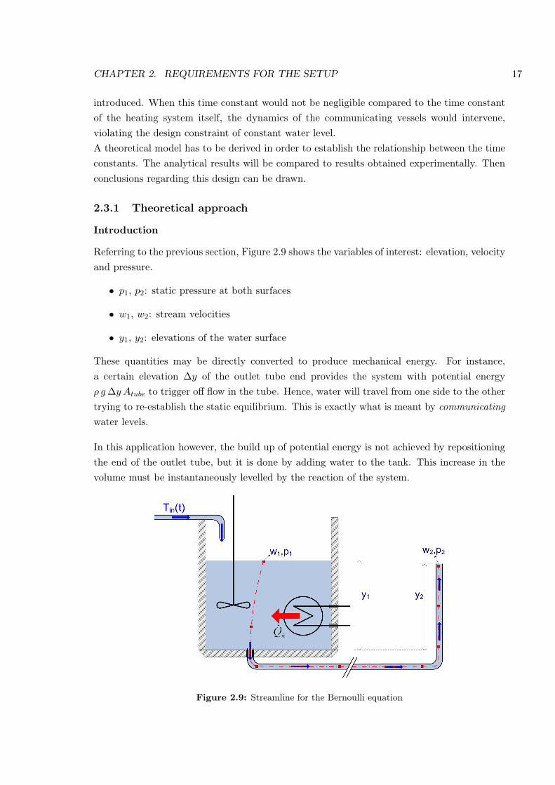
Introduction
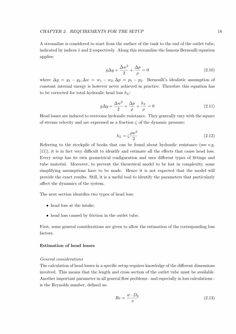
Referring to the previous section, Figure 2.9 shows the variables of interest: elevation, velocityand pressure.
• p1, p2: static pressure at both surfaces
• w1, w2: stream velocities
• y1, y2: elevations of the water surface
These quantities may be directly converted to produce mechanical energy. For instance,a certain elevation ∆y of the outlet tube end provides the system with potential energyρ g ∆y Atube to trigger off flow in the tube. Hence, water will travel from one side to the othertrying to re-establish the static equilibrium. This is exactly what is meant by communicatingwater levels.
In this application however, the build up of potential energy is not achieved by repositioningthe end of the outlet tube, but it is done by adding water to the tank. This increase in thevolume must be instantaneously levelled by the reaction of the system.
Figure 2.9: Streamline for the Bernoulli equation
CHAPTER 2. REQUIREMENTS FOR THE SETUP 18
A streamline is considered to start from the surface of the tank to the end of the outlet tube,indicated by indices 1 and 2 respectively. Along this streamline the famous Bernoulli equationapplies:
g∆y +∆w2
2+
∆p
ρ= 0 (2.10)
where ∆y = y1 − y2,∆w = w1 − w2,∆p = p1 − p2. Bernoulli’s idealistic assumption ofconstant internal energy is however never achieved in practice. Therefore this equation hasto be corrected for total hydraulic head loss hL:
g∆y +∆w2
2+
∆p
ρ+
hL
ρ= 0 (2.11)
Head losses are induced to overcome hydraulic resistance. They generally vary with the squareof stream velocity and are expressed as a fraction ζ of the dynamic pressure:
hL = ζρw2
2(2.12)
Referring to the stockpile of books that can be found about hydraulic resistance (see e.g.[11]), it is in fact very difficult to identify and estimate all the effects that cause head loss.Every setup has its own geometrical configuration and uses different types of fittings andtube material. Moreover, to prevent the theoretical model to be lost in complexity, somesimplifying assumptions have to be made. Hence it is not expected that the model willprovide the exact results. Still, it is a useful tool to identify the parameters that particularlyaffect the dynamics of the system.
The next section identifies two types of head loss:
• head loss at the intake;
• head loss caused by friction in the outlet tube.
First, some general considerations are given to allow the estimation of the corresponding lossfactors.
Estimation of head losses
General considerationsThe calculation of head losses in a specific setup requires knowledge of the different dimensionsinvolved. This means that the length and cross section of the outlet tube must be available.Another important parameter in all general flow problems - and especially in loss calculations -is the Reynolds number, defined as:
Re =w ·Dh
ν(2.13)
CHAPTER 2. REQUIREMENTS FOR THE SETUP 19
The hydraulic diameter Dh is for circular tubes - as in this case - equal to the tube diameter4.ν denotes the dynamic viscosity of water and w the stream velocity [23].At this stage, the dimensions of the outlet tube are themselves parameters of the problem:they must be chosen in such a way that they minimize the hydraulic resistance. Yet, fromprevious section it is known that head losses decrease with the square of the stream velocity.Furthermore, the hydraulic resistance of a tube varies proportionally with its length. Thisleads to the choice of a short tube with large cross sectional area.It is however important to point out that the tube diameter cannot be increased unbounded.In fact this diameter should not be larger than 20 mm, which counts as a practical limit whenit comes down to flexibility. Even this extreme value leads to a long tube. For instance, acontrolled volume of one liter already needs 3.2 m of tube. Thus, it is recommended to windthe tube in a helical coil, irrespective of its dimensions.
Another important issue is the roughness of the tube. This depends on the type of materialand its manufacturing. As plastic tubes will be used in this setup, which are smooth enough,the roughness effect can be ignored.
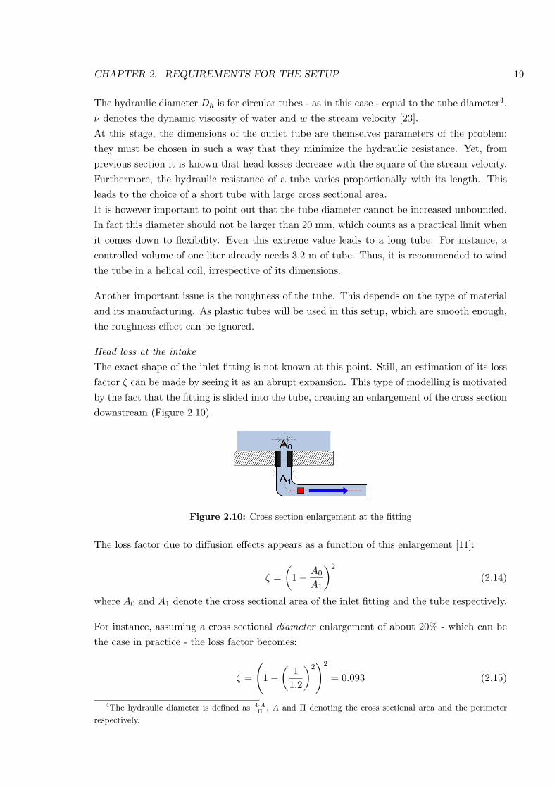
Head loss at the intakeThe exact shape of the inlet fitting is not known at this point. Still, an estimation of its lossfactor ζ can be made by seeing it as an abrupt expansion. This type of modelling is motivatedby the fact that the fitting is slided into the tube, creating an enlargement of the cross sectiondownstream (Figure 2.10).
Figure 2.10: Cross section enlargement at the fitting
The loss factor due to diffusion effects appears as a function of this enlargement [11]:
ζ =(
1− A0
A1
)2
(2.14)
where A0 and A1 denote the cross sectional area of the inlet fitting and the tube respectively.
For instance, assuming a cross sectional diameter enlargement of about 20% - which can bethe case in practice - the loss factor becomes:
ζ =
(1−
(1
1.2
)2)2
= 0.093 (2.15)
4The hydraulic diameter is defined as 4·AΠ
, A and Π denoting the cross sectional area and the perimeter
respectively.
CHAPTER 2. REQUIREMENTS FOR THE SETUP 20
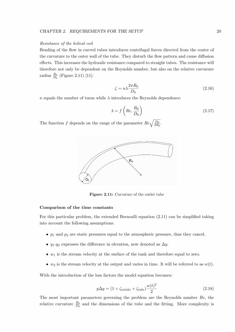
Resistance of the helical coilBending of the flow in curved tubes introduces centrifugal forces directed from the center ofthe curvature to the outer wall of the tube. They disturb the flow pattern and cause diffusioneffects. This increases the hydraulic resistance compared to straight tubes. The resistance willtherefore not only be dependent on the Reynolds number, but also on the relative curvatureradius R0
D0(Figure 2.11) [11]:
ζ = nλ2πR0
Dh(2.16)
n equals the number of turns while λ introduces the Reynolds dependence:
λ = f
(Re,
R0
D0
)(2.17)
The function f depends on the range of the parameter Re√
D02R0
.
Figure 2.11: Curvature of the outlet tube
Comparison of the time constants
For this particular problem, the extended Bernoulli equation (2.11) can be simplified takinginto account the following assumptions:
• p1 and p2 are static pressures equal to the atmospheric pressure, thus they cancel.
• y1-y2 expresses the difference in elevation, now denoted as ∆y.
• w1 is the stream velocity at the surface of the tank and therefore equal to zero.
• w2 is the stream velocity at the output and varies in time. It will be referred to as w(t).
With the introduction of the loss factors the model equation becomes:
g∆y = (1 + ζintake + ζtube)w(t)2
2(2.18)
The most important parameters governing the problem are the Reynolds number Re, therelative curvature R0
D0and the dimensions of the tube and the fitting. More complexity is
CHAPTER 2. REQUIREMENTS FOR THE SETUP 21
introduced as the Reynolds number depends on the stream velocity, which in turn varies withthe relative elevation ∆y. This grade of complexity precludes a general analytic treatment ofthe problem. Nevertheless, with an estimation of the orders of most important parameters,useful conclusions about the behavior of the system can be drawn.An experiment is considered, in which water is added to the tank at a constant rate. Thegoverning parameters and the estimation of their order of magnitude (denoted by Θ) are givennext:
• D0 ≈ Θ(0.02 m) with R0 ≈ 5D0. This results in√
D02R0
≈ 0.32.
• w ≈ Θ(0.1 msec) and D0 lead to Re ≈ Θ(2 · 103)
• L ≈ Θ(3m) is the estimated order of the tube length
• The number of turns n is, with these orders of R0 and L, approximative 5.
With these orders, the parameter Re√
D02R0
≈ Θ(600) leads to a loss factor ζ of the helicaltube [11]:
ζtube = nλ2πR0
D0= n
(2
Re0.65
(D0
2R0
)0.175)
2πR0
D0(2.19)
λ varies with the stream velocity w due to its Reynolds dependence. These variations arehowever small, thus λ is taken constant and equal to 0.01. This leads to ζtube ≈ 1.5. Forthe head loss at the intake, equation (2.15) calculates ζintake = 0.093 for a cross sectionaldiameter enlargement of 20%.
Taking into account these losses, equation (2.18) simplifies to:
g∆y = 2.6w(t)2
2(2.20)
Furthermore, the law of mass conservation applies to the tank which acts as a capacitor:
Atankd∆y
dt= qin − qout or
d∆y
dt=
qin
Atank− Atube
Atankw(t) (2.21)
Differentiating equation (2.20), and substituting d∆ydt into (2.21), a non-linear first order
differential equation appears:
qin
Atank− Atube
Atankw(t) = 2.6
w(t)g
dw(t)dt
(2.22)
Linearizing this equation around w0 allows an estimation of the time constant of the system:
2.6w0
g
dδw(t)dt
− Atube
Atankδw(t) = 0 or τ =
2.6w0
g AtubeAtank
(2.23)
Different parameters affect the magnitude of this time constant and consequently determinethe reaction time of the system.
CHAPTER 2. REQUIREMENTS FOR THE SETUP 22
The time constant is:
• proportional to the overall head loss, which was expected intuitively.
• proportional to the area of the tank. This is expected too because a large area requiresmore inflow in order to build up static pressure ρg∆y.
• inverse proportional to the area of the tube. This parameter also causes a reduction inhead loss of the helical tube.
For example, a cross sectional tank diameter of ten times the diameter of the inlet tube, leadsto a time constant τ = 2.7 sec when w0 = 0.1 m
sec . Comparing this time constant to the oneof the heating tank system5, we obtain
τcmv
τhts≈ τcmv
Vqout
=τcmv
LSw0S
=2.7
3/0.1= 9% (2.24)
This ratio indicates that both time constants have a different order of magnitude.
2.3.2 Results
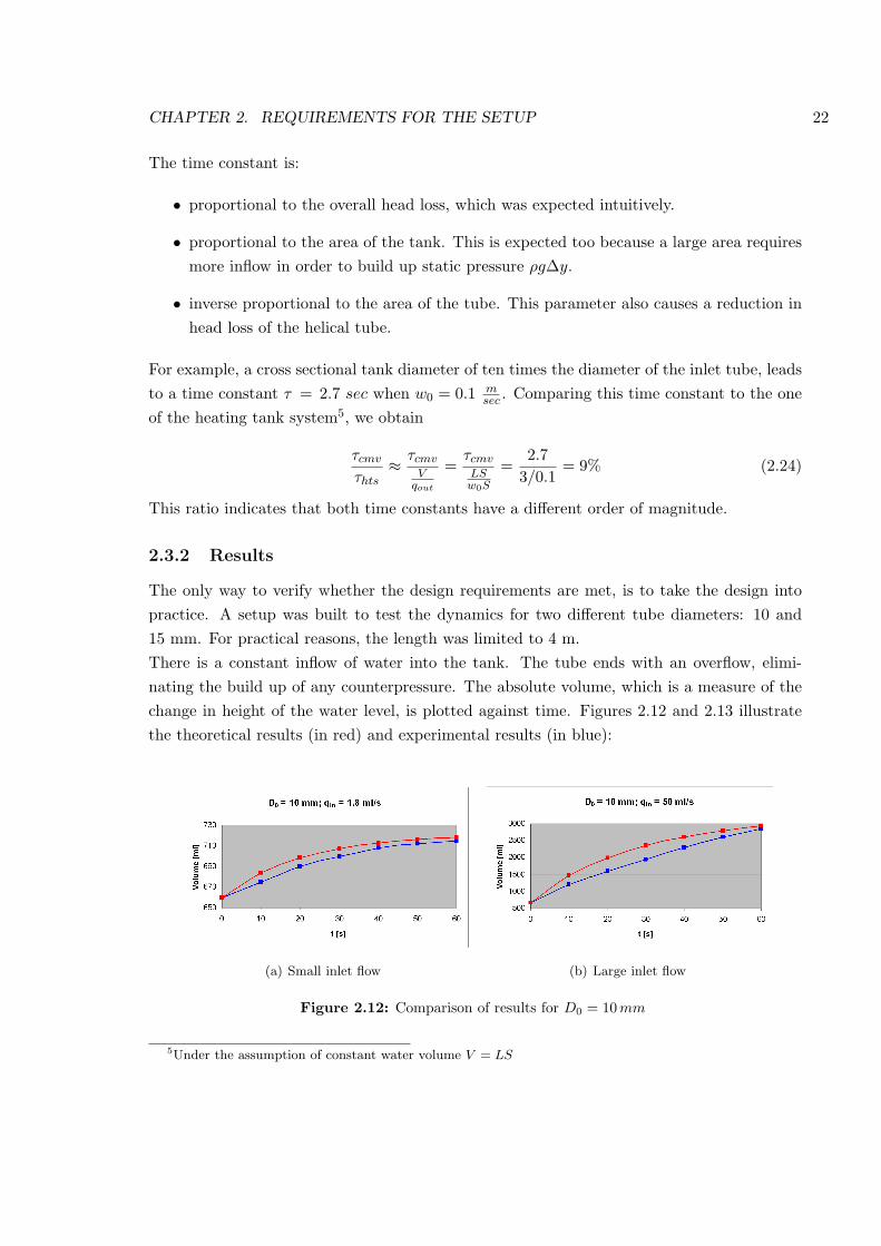
The only way to verify whether the design requirements are met, is to take the design intopractice. A setup was built to test the dynamics for two different tube diameters: 10 and15 mm. For practical reasons, the length was limited to 4 m.There is a constant inflow of water into the tank. The tube ends with an overflow, elimi-nating the build up of any counterpressure. The absolute volume, which is a measure of thechange in height of the water level, is plotted against time. Figures 2.12 and 2.13 illustratethe theoretical results (in red) and experimental results (in blue):
(a) Small inlet flow (b) Large inlet flow
Figure 2.12: Comparison of results for D0 = 10 mm
5Under the assumption of constant water volume V = LS
CHAPTER 2. REQUIREMENTS FOR THE SETUP 23
(a) Small inlet flow (b) Large inlet flow
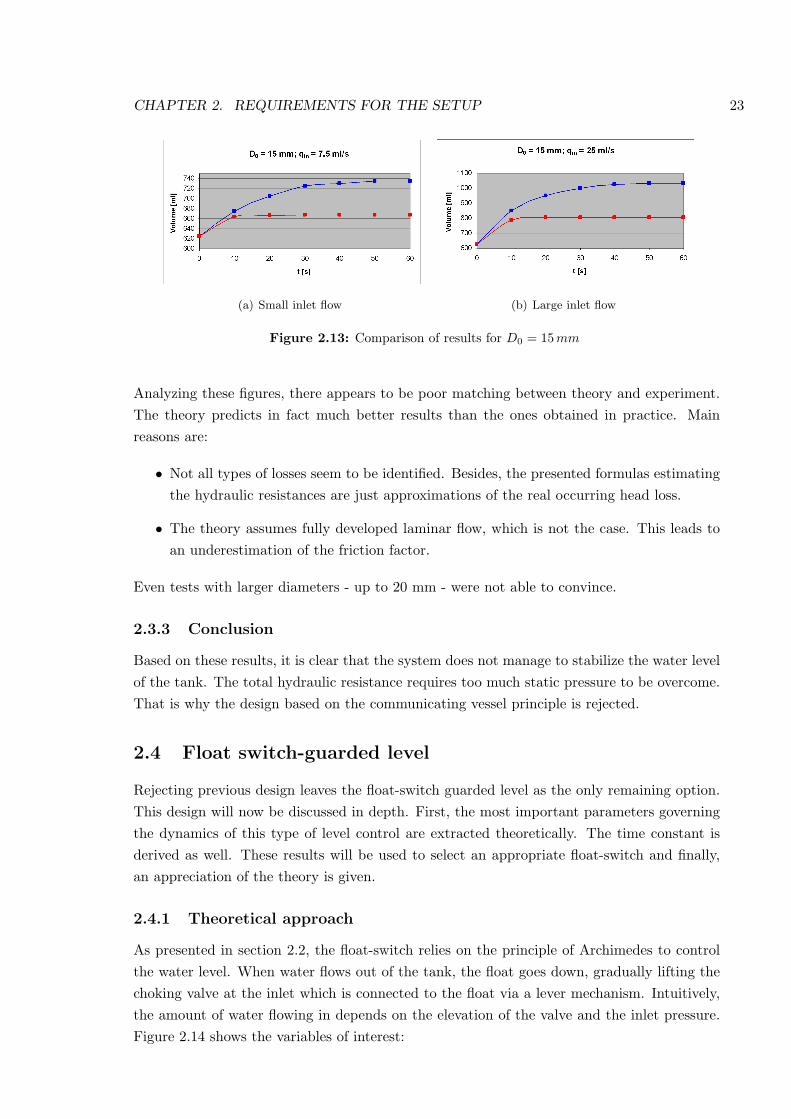
Figure 2.13: Comparison of results for D0 = 15 mm
Analyzing these figures, there appears to be poor matching between theory and experiment.The theory predicts in fact much better results than the ones obtained in practice. Mainreasons are:
• Not all types of losses seem to be identified. Besides, the presented formulas estimatingthe hydraulic resistances are just approximations of the real occurring head loss.
• The theory assumes fully developed laminar flow, which is not the case. This leads toan underestimation of the friction factor.
Even tests with larger diameters - up to 20 mm - were not able to convince.
2.3.3 Conclusion
Based on these results, it is clear that the system does not manage to stabilize the water levelof the tank. The total hydraulic resistance requires too much static pressure to be overcome.That is why the design based on the communicating vessel principle is rejected.
2.4 Float switch-guarded level
Rejecting previous design leaves the float-switch guarded level as the only remaining option.This design will now be discussed in depth. First, the most important parameters governingthe dynamics of this type of level control are extracted theoretically. The time constant isderived as well. These results will be used to select an appropriate float-switch and finally,an appreciation of the theory is given.
2.4.1 Theoretical approach
As presented in section 2.2, the float-switch relies on the principle of Archimedes to controlthe water level. When water flows out of the tank, the float goes down, gradually lifting thechoking valve at the inlet which is connected to the float via a lever mechanism. Intuitively,the amount of water flowing in depends on the elevation of the valve and the inlet pressure.Figure 2.14 shows the variables of interest:
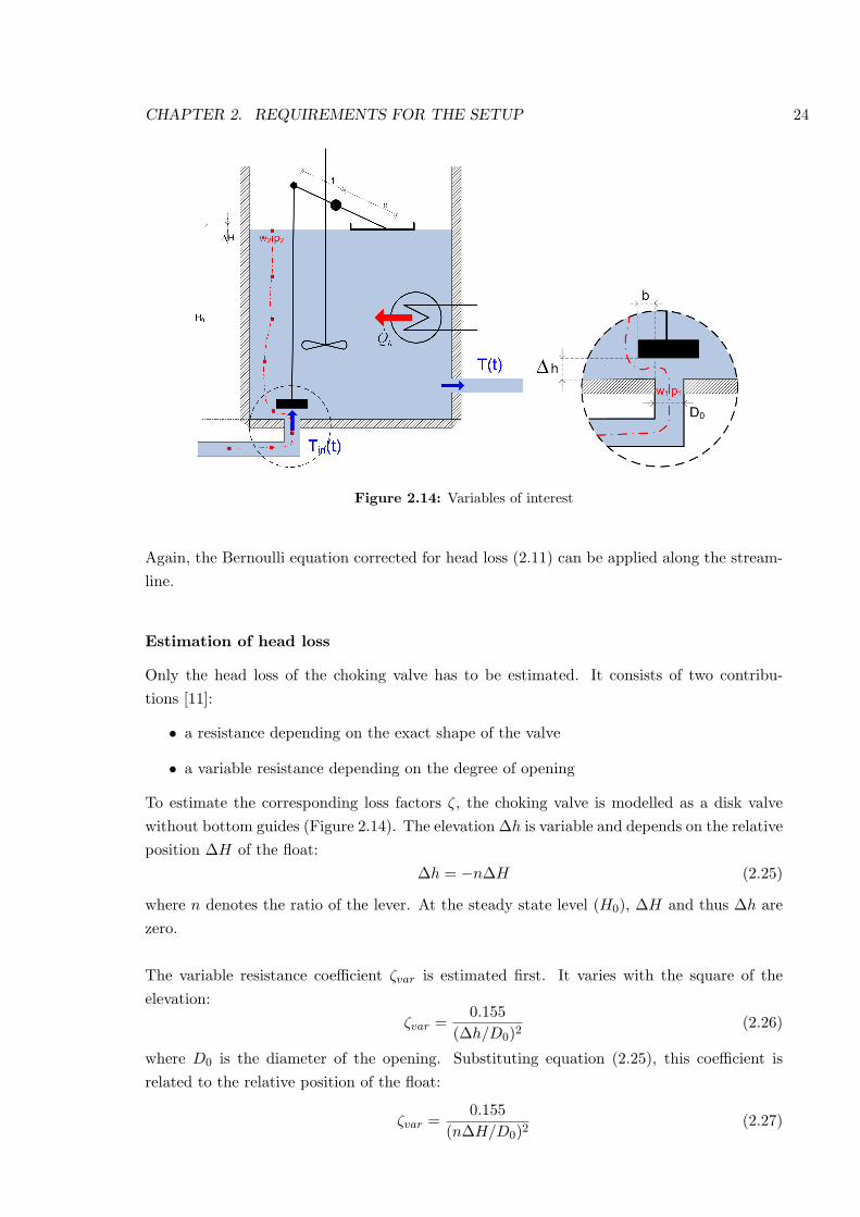
CHAPTER 2. REQUIREMENTS FOR THE SETUP 24
Figure 2.14: Variables of interest
Again, the Bernoulli equation corrected for head loss (2.11) can be applied along the stream-line.
Estimation of head loss
Only the head loss of the choking valve has to be estimated. It consists of two contribu-tions [11]:
• a resistance depending on the exact shape of the valve
• a variable resistance depending on the degree of opening
To estimate the corresponding loss factors ζ, the choking valve is modelled as a disk valvewithout bottom guides (Figure 2.14). The elevation ∆h is variable and depends on the relativeposition ∆H of the float:
∆h = −n∆H (2.25)
where n denotes the ratio of the lever. At the steady state level (H0), ∆H and thus ∆h arezero.
The variable resistance coefficient ζvar is estimated first. It varies with the square of theelevation:
ζvar =0.155
(∆h/D0)2(2.26)
where D0 is the diameter of the opening. Substituting equation (2.25), this coefficient isrelated to the relative position of the float:
ζvar =0.155
(n∆H/D0)2(2.27)
CHAPTER 2. REQUIREMENTS FOR THE SETUP 25
The parameters determining the shape-dependent resistance of the valve are the width of thetray flange b and the opening diameter D0:
ζfix = 0.55 + 4[(
b
D0
)− 0.1
](2.28)
With these estimations, the total head loss of the choking valve appears as a function of ∆H:
ζtot = ζfix + ζvar = 0.55 + 4[(
b
D0
)− 0.1
]+
0.155(n∆H/D0)2
(2.29)
Comparison of the time constants
The Bernoulli equation applied along the streamline illustrated in Figure 2.14 can be simplifiedconsidering:
• ∆p as the overpressure of the inflow
• ∆y = − (H0 + ∆H) as the oriented difference in height between the two end points ofthe streamline
• ∆w2 = w21 as the difference in dynamic pressure since w2 is approximately zero at the
surface of the tank. w1 varies in time and will be expressed as w(t).
Introducing the loss factor, we obtain:
∆p
ρ+
w(t)2
2= (ζfix + ζvar)
w(t)2
2+ g (H0 + ∆H)
or∆p
ρ= (ζfix + ζvar − 1)
w(t)2
2+ g (H0 + ∆H) (2.30)
Recalling equation (2.21), the change in the tank volume now becomes:
Atankd∆H
dt= (πD0∆h) w(t)− qout (2.31)
Solving equation (2.30) for w(t)6:
w(t) =
√2
ζtot − 1
(∆p
ρ− g (H0 + ∆H)
)(2.32)
and substituting it into (2.31), with (2.25) taken into account, a non-linear differential equa-tion results:
Atankd∆H
dt= − (πD0n∆H)
√2
ζtot − 1
(∆p
ρ− g (H0 + ∆H)
)− qout (2.33)
More complexity is introduced as ζtot also depends on ∆H, relationship given by equation(2.29). Nevertheless, to get an idea about the time constant of the system, some simplifyingassumptions are made:
6Under the assumption of ζtot > 1 which is certainly the case for small values of ∆H as equation (2.26)
indicates.
CHAPTER 2. REQUIREMENTS FOR THE SETUP 26
1. ∆p corresponds to the supply pressure of the water distribution system, typically ≈Θ(2.105 Pa). Hence, H0 + ∆H ≈ Θ(0.1 m) is small compared to ∆p/ρ
g ≈ Θ(20m).
2. Estimating the dimensions of the choking valve, ζfix (2.28) and ζvar (2.26) can becompared to each other, simplifying ζtot. The diameter of the opening is very small, evenD0 ≈ Θ(3mm) is probably an overestimation. Referring to (2.26), small fluctuationson the water level cause high loss factors ζvar. Therefore, taking ∆h ≈ D0
7 leads to anoverestimation of the loss factor ζvar. As this is a conservative approximation, it can bemade though.
Hence, the ∆H-dependence in ζtot disappears:
ζtot = ζfix + ζvar ≈ 0.55 + 4[(
b
D0
)− 0.1
]+
0.155n2
(2.34)
and (2.33) simplifies to a linear differential equation:
Atankd∆H
dt= − (πD0n∆H)
√(2
ζtot − 1∆p
ρ
)− qout (2.35)
whose time constant can be derived immediately:
τ =Atank
πD0n
√(2
ζtot−1∆pρ
) (2.36)
The most important parameters governing the dynamics are:
• The area of the tank. Reducing this area will intensify the sensitivity to level fluctua-tions, and thus leads to faster dynamics.
• The diameter of the opening. Given the elevation of the choking valve, more water willflow in when the diameter is large.
• The ratio of the lever mechanism. If n is large, even a small change in level will alreadylead to a significant lift of the valve.
• The supply pressure of the water distribution system, which is maybe the most impor-tant parameter. If the pressure is low, this will result in a large time constant due to thesmall amount of energy available to overcome head loss. Moreover, very low pressurecan even cause a permanent decrease of the water level when too much liquid flows outof the tank.
Except for the area of the tank, these parameters will also determine the steady state decreaseof the water level for a given outflow:
∆H∗ =−qout
πD0n
√(2
ζtot−1∆pρ
) (2.37)
To give an appreciation, it is interesting to look at some numerical values. Taking for instance:7If D0 = 3 mm and n = 3, the decrease ∆H of the water level is only 1 mm!
CHAPTER 2. REQUIREMENTS FOR THE SETUP 27
• D0 = 3 mm, b = 2 mm and n = 3 as characteristic dimensions of the float switch valveand lever mechanism
• ∆p = 2 bar as the supply pressure
• and Atank = 0.01 m2
the overall loss factor results from (2.34):
ζtot ≈ 0.55 + 4[(
23
)− 0.1
]+
0.15532
= 2.83
With this expression, the time constant is calculated as in (2.36):
τ =0.01
0.003 · 3π
√(2
2.83−12·105
103
) = 0.02 sec
which is extremely small, partly due to the chosen values, partly due to the assumption ofconstant head loss (independent of ∆H).Finally, assuming an outflow of 2l/min, the steady state decrease of the water level is:
∆H∗ =−2/60
0.003 · 3π
√(2
2.83−12·105
103
) = −0.08 mm
which is hardly visible.
2.4.2 Conclusion
Though these numeric values result from the simplified linear system, they indicate thatthe time constant and steady state level decrease can be very small in the real setup. Thetheoretical results show that only a few parameters are determinant for the success of thefloat-switch level control. Fortunately, we have found a level switch which has the rightcharacteristic dimensions. When the design was taken into practice, almost no fluctuationon the water level was visible, as predicted theoretically. Also, the setup is located on theground floor to profit maximally from the supply pressure.
Chapter 3
Mechanical and electrical
implementation
3.1 Flow Control
3.1.1 Types of actuators
To compare the performance of the three real-time controllers, it is important that the con-trolled actuator applies the desired flow accurately. This leaves the tank temperature only tobe manipulated by the control actions themselves and not by the arbitrariness of the device.Hence a good basis for comparison is created.
Generally, flow controlling devices can be split up into two categories:
1. Passive actuators: for this type of devices the flow does not depend only on actuatoractions, but also on external influences.
2. Active actuators: these type of devices force the liquid to flow, irrespective of theconfiguration of the setup.
The two types differ significantly in the accuracy they can achieve. Taking for instance anelectromagnetic valve as a common example in the first category, it is clear that the openingof the valve itself does not trigger off flow. It is the pressure difference however that providesthe energy needed to overcome hydraulic resistance. That is why an electromagnetic valveby itself can not impose a certain flow on the process.
An alternative solution is to switch from open loop to closed loop control. In this case, asensor registers the flow continuously to provide feedback for a controller. There are howevertwo major disadvantages of this approach. Firstly, most flow sensors are quite expensive anddo not work well for small inputs. Secondly, electromagnetic valves in general provide onlyON-OFF regulation. The reason lies in the electromagnetic principles the valve relies on.Hence in this case, only a relay controller can be used. This complicates flow measurementeven more. Taking into account all these considerations, valves seem not fit to be used forour purpose.
28
CHAPTER 3. MECHANICAL AND ELECTRICAL IMPLEMENTATION 29
Somewhere between active and passive actuators are the non-volumetric pumps. The relationbetween pump speed and flow still depends on the discharge head. That is why non-volumetricpumps are typically used in large flow applications and are not well suited for our application(small flows). A solution is the use of a choking valve at the outlet increasing the dischargehead and consequently influencing the static characteristic of the pump. However, this ar-tificial measure of dumping energy is in fact not very elegant from the engineering point ofview.
Another drawback comes with the speed regulation. In standard applications - for instancethe circulation pump of the central heating - these non-volumetric pumps are equipped with asingle phase electric motor, designed to operate at the network frequency. Compared to DC-motors, strategies for controlling this type of motors are less evident. Finally, non-volumetricpumps in combination with a choking valve can suffer from back flow when suddenly decreas-ing the speed. This is not desired either.
On the contrary, volumetric pumps belong to the category of active actuators and thereforeoffer a lot of advantages. Peristaltic pumps are the most widely used in practice (e.g. dosingapplications). Due to roller compression of the tube, a constant volume of liquid is transferredfrom the pump inlet to the outlet at every rotation, without the risk of backflow. This makesthe characteristic between flow and speed perfectly linear and only determined by volumetricproperties. Compared to membrane pumps, they do not have valves, thus no maintenance isrequired. All these advantages explain why in this application a peristaltic pump was chosen.For more information about pumps, we refer to [16] and [9].
3.1.2 Controlling the flow
With the linear relation between flow and speed, the problem of flow control shifts to speedcontrol. In this application a DC-motor is most suitable because it profits from high startingtorques and offers a simple relation between armature voltage and speed [13]:
V = RaIa + LadIa
dt+ Ea (3.1)
with
• V : the armature voltage;
• Ia: the current through the motor;
• Ra and La: the resistance and inductance of the armature respectively;
• Ea: the back emf generated in the armature.
For a permanent magnet DC-motor the flux φ remains constant, resulting in:
Ea = kφΩ = KΩ (3.2)
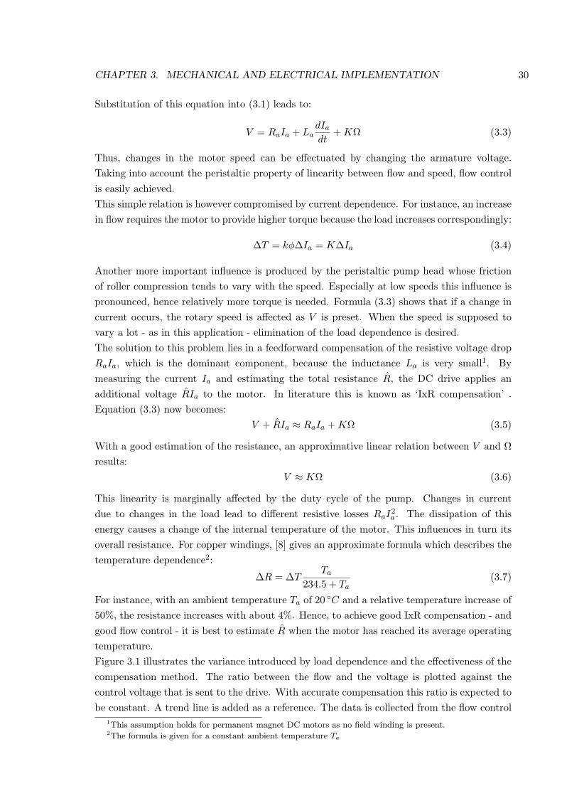
CHAPTER 3. MECHANICAL AND ELECTRICAL IMPLEMENTATION 30
Substitution of this equation into (3.1) leads to:
V = RaIa + LadIa
dt+ KΩ (3.3)
Thus, changes in the motor speed can be effectuated by changing the armature voltage.Taking into account the peristaltic property of linearity between flow and speed, flow controlis easily achieved.This simple relation is however compromised by current dependence. For instance, an increasein flow requires the motor to provide higher torque because the load increases correspondingly:
∆T = kφ∆Ia = K∆Ia (3.4)
Another more important influence is produced by the peristaltic pump head whose frictionof roller compression tends to vary with the speed. Especially at low speeds this influence ispronounced, hence relatively more torque is needed. Formula (3.3) shows that if a change incurrent occurs, the rotary speed is affected as V is preset. When the speed is supposed tovary a lot - as in this application - elimination of the load dependence is desired.The solution to this problem lies in a feedforward compensation of the resistive voltage dropRaIa, which is the dominant component, because the inductance La is very small1. Bymeasuring the current Ia and estimating the total resistance R, the DC drive applies anadditional voltage RIa to the motor. In literature this is known as ‘IxR compensation’ .Equation (3.3) now becomes:
V + RIa ≈ RaIa + KΩ (3.5)
With a good estimation of the resistance, an approximative linear relation between V and Ωresults:
V ≈ KΩ (3.6)
This linearity is marginally affected by the duty cycle of the pump. Changes in currentdue to changes in the load lead to different resistive losses RaI
2a . The dissipation of this
energy causes a change of the internal temperature of the motor. This influences in turn itsoverall resistance. For copper windings, [8] gives an approximate formula which describes thetemperature dependence2:
∆R = ∆TTa
234.5 + Ta(3.7)
For instance, with an ambient temperature Ta of 20 C and a relative temperature increase of50%, the resistance increases with about 4%. Hence, to achieve good IxR compensation - andgood flow control - it is best to estimate R when the motor has reached its average operatingtemperature.Figure 3.1 illustrates the variance introduced by load dependence and the effectiveness of thecompensation method. The ratio between the flow and the voltage is plotted against thecontrol voltage that is sent to the drive. With accurate compensation this ratio is expected tobe constant. A trend line is added as a reference. The data is collected from the flow control
1This assumption holds for permanent magnet DC motors as no field winding is present.2The formula is given for a constant ambient temperature Ta
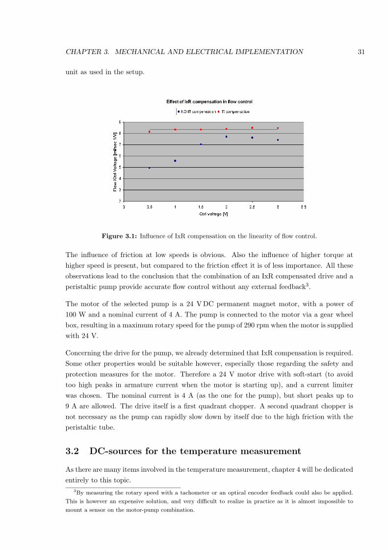
CHAPTER 3. MECHANICAL AND ELECTRICAL IMPLEMENTATION 31
unit as used in the setup.
Figure 3.1: Influence of IxR compensation on the linearity of flow control.
The influence of friction at low speeds is obvious. Also the influence of higher torque athigher speed is present, but compared to the friction effect it is of less importance. All theseobservations lead to the conclusion that the combination of an IxR compensated drive and aperistaltic pump provide accurate flow control without any external feedback3.
The motor of the selected pump is a 24 V DC permanent magnet motor, with a power of100 W and a nominal current of 4 A. The pump is connected to the motor via a gear wheelbox, resulting in a maximum rotary speed for the pump of 290 rpm when the motor is suppliedwith 24 V.
Concerning the drive for the pump, we already determined that IxR compensation is required.Some other properties would be suitable however, especially those regarding the safety andprotection measures for the motor. Therefore a 24 V motor drive with soft-start (to avoidtoo high peaks in armature current when the motor is starting up), and a current limiterwas chosen. The nominal current is 4 A (as the one for the pump), but short peaks up to9 A are allowed. The drive itself is a first quadrant chopper. A second quadrant chopper isnot necessary as the pump can rapidly slow down by itself due to the high friction with theperistaltic tube.
3.2 DC-sources for the temperature measurement
As there are many items involved in the temperature measurement, chapter 4 will be dedicatedentirely to this topic.
3By measuring the rotary speed with a tachometer or an optical encoder feedback could also be applied.
This is however an expensive solution, and very difficult to realize in practice as it is almost impossible to
mount a sensor on the motor-pump combination.
CHAPTER 3. MECHANICAL AND ELECTRICAL IMPLEMENTATION 32
For the measurement circuits, fixed DC-sources are required: +15 and -15 V to feed theoperational amplifiers (op amps), 5 V for the excitation of the sensor and 9 V for the mixer.In order to obtain these voltages, a 2x15 V AC print transformer is used. Thus, in amplitudevalues, the transformer supplies approximately +21 and -21 V AC (using the center tap asground). A rectifier bridge is used together with capacitors to smooth the ripple, resulting ina 19 V DC. This DC source is used to feed +15 V, -15 V, +5 V and +9 V voltage regulators,integrated circuits (ic) that supply a very stable DC voltage. Extra capacitors are added tothe output of the ic’s to insure even more stability (Figure 3.2).
Figure 3.2: DC-sources for temperature measurement
3.3 Data acquisition
3.3.1 Requirements
In the search for a data acquisition board (DAQ), attention must be payed to three issues.The most important one is that it should have enough input and outputs, analog as well asdigital. The second one concerns the maximum sampling rate that can be achieved, while thethird one regards the resolution.
In the setup, three temperature measurements have to be taken simultaneously. These arevoltages in the 0-10 V range, sampled by the DAQ-board and converted into a bit sequenceof a certain length, depending on the resolution. For instance, if the board has a 12-bitresolution, the minimum voltage difference it can distinguish is:
(∆V )min =10 V
212= 2.44 · 10−3 V (3.8)
corresponding to a temperature change of:
∆T = 50 C∆V
10 V= 0.0122 C (3.9)
This resolution outreaches the overall temperature accuracy by far, hence, a 12-bit DAQ-board is surely good enough for this application.
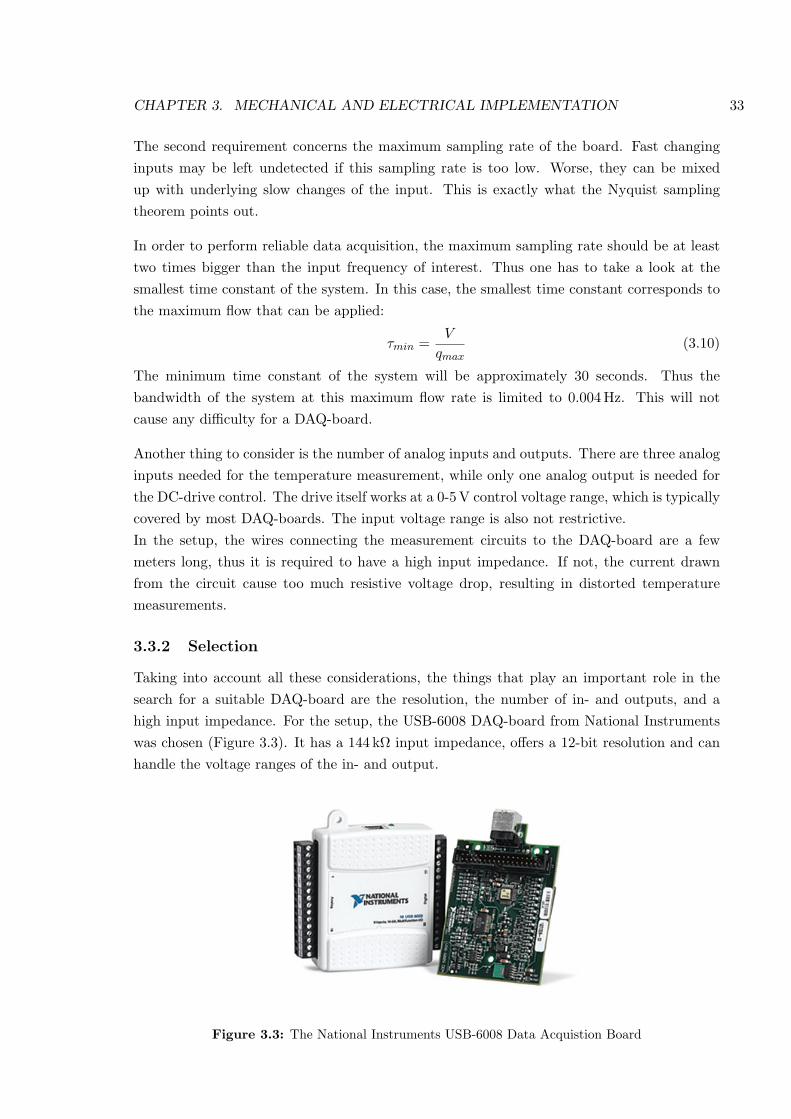
CHAPTER 3. MECHANICAL AND ELECTRICAL IMPLEMENTATION 33
The second requirement concerns the maximum sampling rate of the board. Fast changinginputs may be left undetected if this sampling rate is too low. Worse, they can be mixedup with underlying slow changes of the input. This is exactly what the Nyquist samplingtheorem points out.
In order to perform reliable data acquisition, the maximum sampling rate should be at leasttwo times bigger than the input frequency of interest. Thus one has to take a look at thesmallest time constant of the system. In this case, the smallest time constant corresponds tothe maximum flow that can be applied:
τmin =V
qmax(3.10)
The minimum time constant of the system will be approximately 30 seconds. Thus thebandwidth of the system at this maximum flow rate is limited to 0.004 Hz. This will notcause any difficulty for a DAQ-board.
Another thing to consider is the number of analog inputs and outputs. There are three analoginputs needed for the temperature measurement, while only one analog output is needed forthe DC-drive control. The drive itself works at a 0-5 V control voltage range, which is typicallycovered by most DAQ-boards. The input voltage range is also not restrictive.In the setup, the wires connecting the measurement circuits to the DAQ-board are a fewmeters long, thus it is required to have a high input impedance. If not, the current drawnfrom the circuit cause too much resistive voltage drop, resulting in distorted temperaturemeasurements.
3.3.2 Selection
Taking into account all these considerations, the things that play an important role in thesearch for a suitable DAQ-board are the resolution, the number of in- and outputs, and ahigh input impedance. For the setup, the USB-6008 DAQ-board from National Instrumentswas chosen (Figure 3.3). It has a 144 kΩ input impedance, offers a 12-bit resolution and canhandle the voltage ranges of the in- and output.
Figure 3.3: The National Instruments USB-6008 Data Acquistion Board
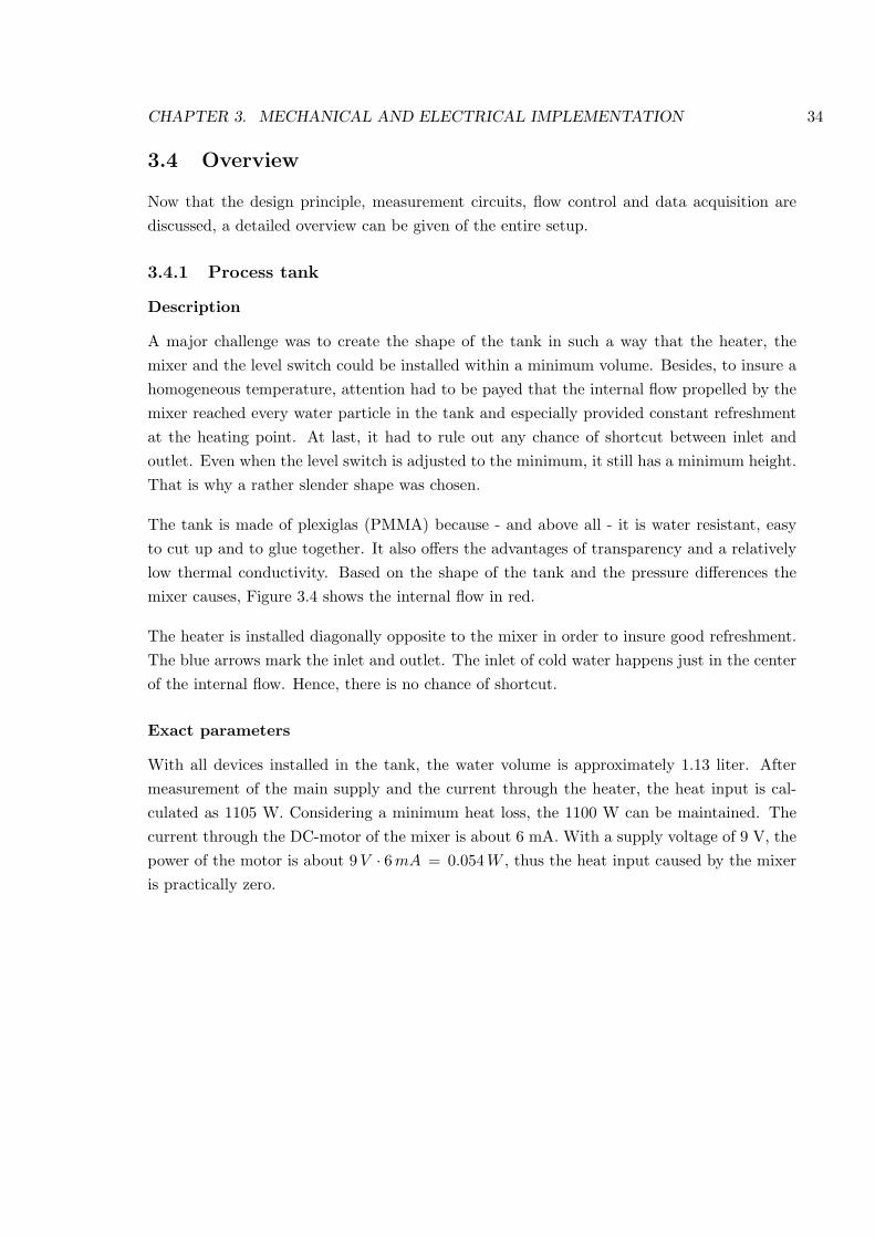
CHAPTER 3. MECHANICAL AND ELECTRICAL IMPLEMENTATION 34
3.4 Overview
Now that the design principle, measurement circuits, flow control and data acquisition arediscussed, a detailed overview can be given of the entire setup.
3.4.1 Process tank
Description
A major challenge was to create the shape of the tank in such a way that the heater, themixer and the level switch could be installed within a minimum volume. Besides, to insure ahomogeneous temperature, attention had to be payed that the internal flow propelled by themixer reached every water particle in the tank and especially provided constant refreshmentat the heating point. At last, it had to rule out any chance of shortcut between inlet andoutlet. Even when the level switch is adjusted to the minimum, it still has a minimum height.That is why a rather slender shape was chosen.
The tank is made of plexiglas (PMMA) because - and above all - it is water resistant, easyto cut up and to glue together. It also offers the advantages of transparency and a relativelylow thermal conductivity. Based on the shape of the tank and the pressure differences themixer causes, Figure 3.4 shows the internal flow in red.
The heater is installed diagonally opposite to the mixer in order to insure good refreshment.The blue arrows mark the inlet and outlet. The inlet of cold water happens just in the centerof the internal flow. Hence, there is no chance of shortcut.
Exact parameters
With all devices installed in the tank, the water volume is approximately 1.13 liter. Aftermeasurement of the main supply and the current through the heater, the heat input is cal-culated as 1105 W. Considering a minimum heat loss, the 1100 W can be maintained. Thecurrent through the DC-motor of the mixer is about 6 mA. With a supply voltage of 9 V, thepower of the motor is about 9V · 6 mA = 0.054 W , thus the heat input caused by the mixeris practically zero.
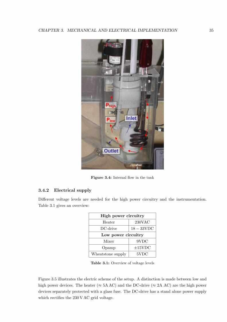
CHAPTER 3. MECHANICAL AND ELECTRICAL IMPLEMENTATION 35
Figure 3.4: Internal flow in the tank
3.4.2 Electrical supply
Different voltage levels are needed for the high power circuitry and the instrumentation.Table 3.1 gives an overview:
High power circuitry
Heater 230VAC
DC-drive 18− 33VDC
Low power circuitry
Mixer 9VDC
Opamp ±15VDC
Wheatstone supply 5VDC
Table 3.1: Overview of voltage levels
Figure 3.5 illustrates the electric scheme of the setup. A distinction is made between low andhigh power devices. The heater (≈ 5A AC) and the DC-drive (≈ 2A AC) are the high powerdevices separately protected with a glass fuse. The DC-drive has a stand alone power supplywhich rectifies the 230 V AC grid voltage.
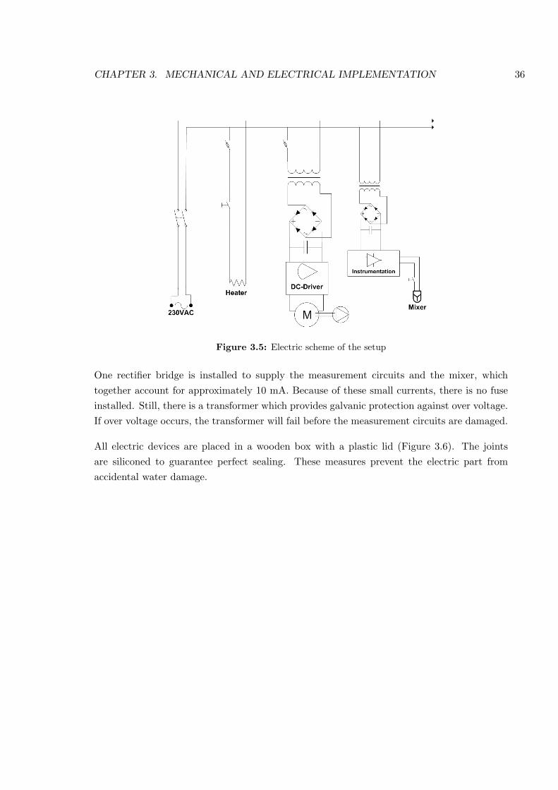
CHAPTER 3. MECHANICAL AND ELECTRICAL IMPLEMENTATION 36
Figure 3.5: Electric scheme of the setup
One rectifier bridge is installed to supply the measurement circuits and the mixer, whichtogether account for approximately 10 mA. Because of these small currents, there is no fuseinstalled. Still, there is a transformer which provides galvanic protection against over voltage.If over voltage occurs, the transformer will fail before the measurement circuits are damaged.
All electric devices are placed in a wooden box with a plastic lid (Figure 3.6). The jointsare siliconed to guarantee perfect sealing. These measures prevent the electric part fromaccidental water damage.
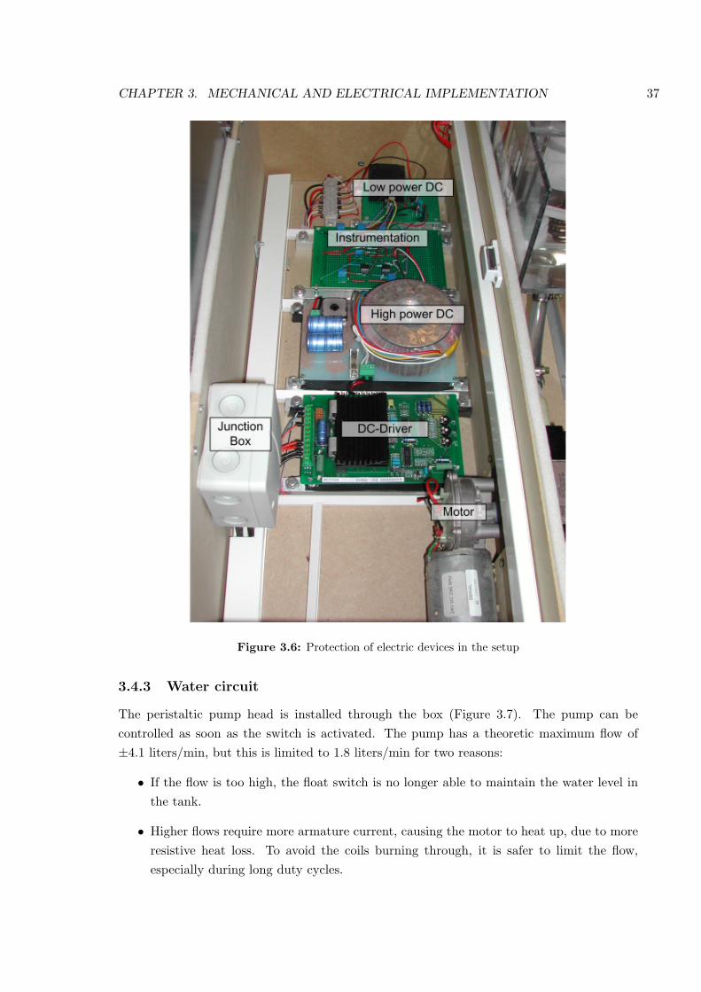
CHAPTER 3. MECHANICAL AND ELECTRICAL IMPLEMENTATION 37
Figure 3.6: Protection of electric devices in the setup
3.4.3 Water circuit
The peristaltic pump head is installed through the box (Figure 3.7). The pump can becontrolled as soon as the switch is activated. The pump has a theoretic maximum flow of±4.1 liters/min, but this is limited to 1.8 liters/min for two reasons:
• If the flow is too high, the float switch is no longer able to maintain the water level inthe tank.
• Higher flows require more armature current, causing the motor to heat up, due to moreresistive heat loss. To avoid the coils burning through, it is safer to limit the flow,especially during long duty cycles.
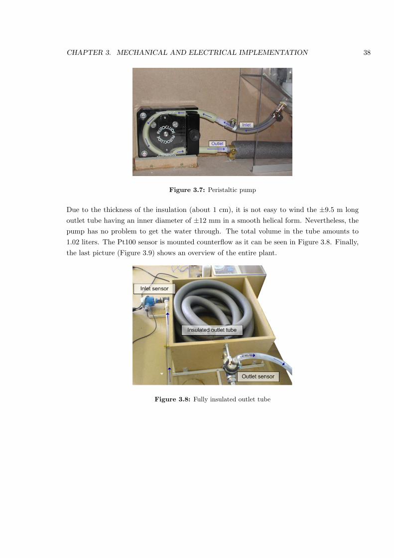
CHAPTER 3. MECHANICAL AND ELECTRICAL IMPLEMENTATION 38
Figure 3.7: Peristaltic pump
Due to the thickness of the insulation (about 1 cm), it is not easy to wind the ±9.5 m longoutlet tube having an inner diameter of ±12 mm in a smooth helical form. Nevertheless, thepump has no problem to get the water through. The total volume in the tube amounts to1.02 liters. The Pt100 sensor is mounted counterflow as it can be seen in Figure 3.8. Finally,the last picture (Figure 3.9) shows an overview of the entire plant.
Figure 3.8: Fully insulated outlet tube
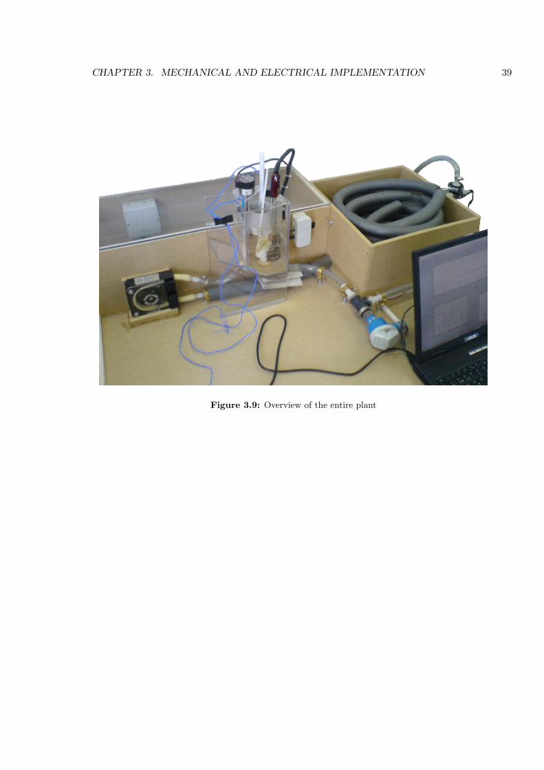
CHAPTER 3. MECHANICAL AND ELECTRICAL IMPLEMENTATION 39
Figure 3.9: Overview of the entire plant
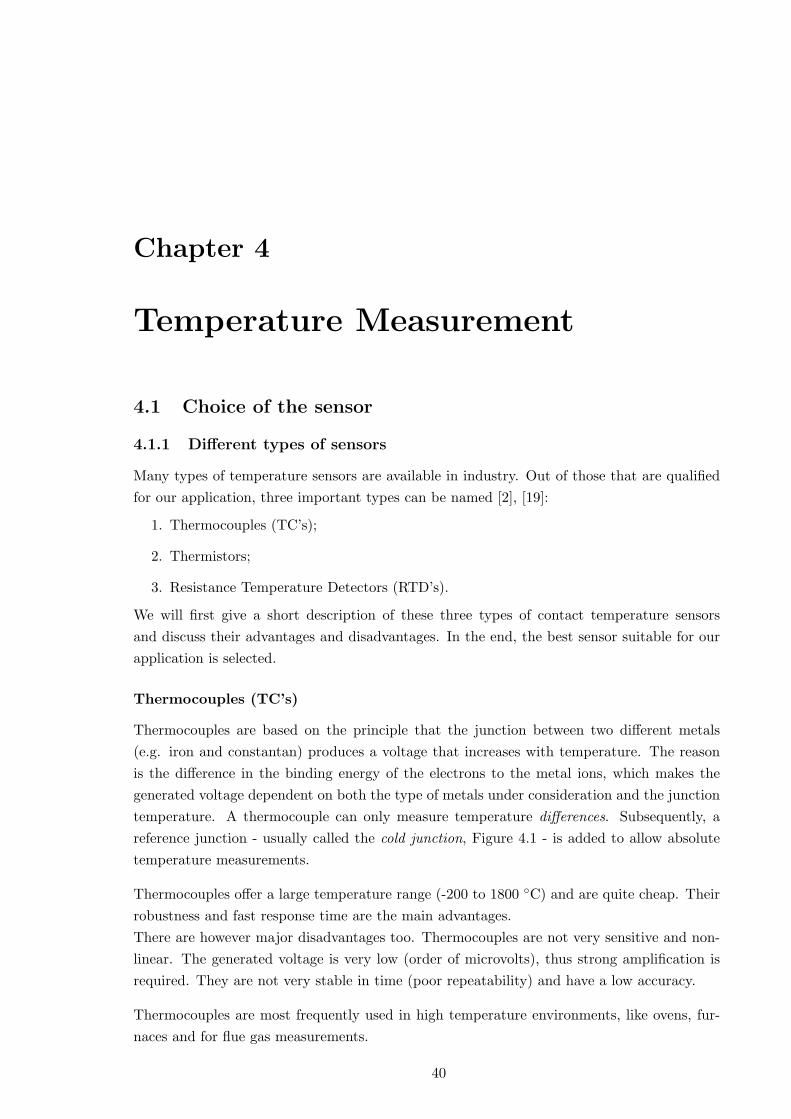
Chapter 4
Temperature Measurement
4.1 Choice of the sensor
4.1.1 Different types of sensors
Many types of temperature sensors are available in industry. Out of those that are qualifiedfor our application, three important types can be named [2], [19]:
1. Thermocouples (TC’s);
2. Thermistors;
3. Resistance Temperature Detectors (RTD’s).
We will first give a short description of these three types of contact temperature sensorsand discuss their advantages and disadvantages. In the end, the best sensor suitable for ourapplication is selected.
Thermocouples (TC’s)
Thermocouples are based on the principle that the junction between two different metals(e.g. iron and constantan) produces a voltage that increases with temperature. The reasonis the difference in the binding energy of the electrons to the metal ions, which makes thegenerated voltage dependent on both the type of metals under consideration and the junctiontemperature. A thermocouple can only measure temperature differences. Subsequently, areference junction - usually called the cold junction, Figure 4.1 - is added to allow absolutetemperature measurements.
Thermocouples offer a large temperature range (-200 to 1800 C) and are quite cheap. Theirrobustness and fast response time are the main advantages.There are however major disadvantages too. Thermocouples are not very sensitive and non-linear. The generated voltage is very low (order of microvolts), thus strong amplification isrequired. They are not very stable in time (poor repeatability) and have a low accuracy.
Thermocouples are most frequently used in high temperature environments, like ovens, fur-naces and for flue gas measurements.
40
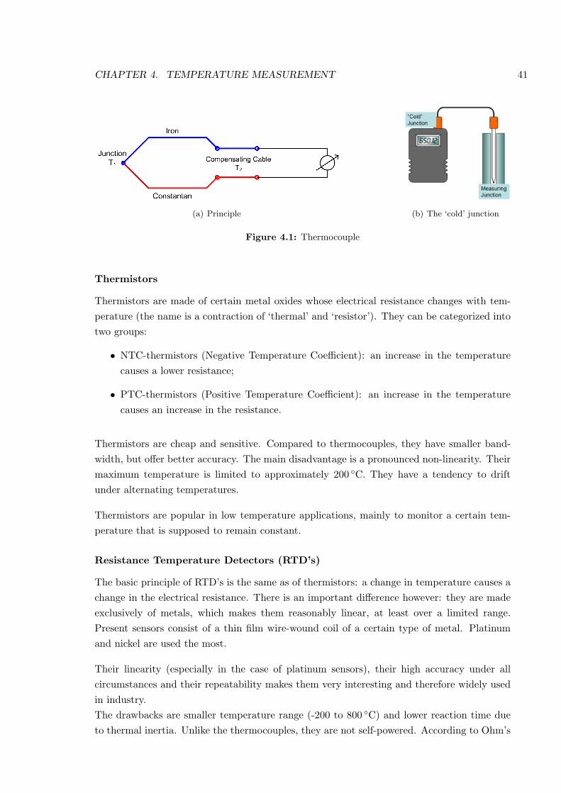
CHAPTER 4. TEMPERATURE MEASUREMENT 41
(a) Principle (b) The ‘cold’ junction
Figure 4.1: Thermocouple
Thermistors
Thermistors are made of certain metal oxides whose electrical resistance changes with tem-perature (the name is a contraction of ‘thermal’ and ‘resistor’). They can be categorized intotwo groups:
• NTC-thermistors (Negative Temperature Coefficient): an increase in the temperaturecauses a lower resistance;
• PTC-thermistors (Positive Temperature Coefficient): an increase in the temperaturecauses an increase in the resistance.
Thermistors are cheap and sensitive. Compared to thermocouples, they have smaller band-width, but offer better accuracy. The main disadvantage is a pronounced non-linearity. Theirmaximum temperature is limited to approximately 200 C. They have a tendency to driftunder alternating temperatures.
Thermistors are popular in low temperature applications, mainly to monitor a certain tem-perature that is supposed to remain constant.
Resistance Temperature Detectors (RTD’s)
The basic principle of RTD’s is the same as of thermistors: a change in temperature causes achange in the electrical resistance. There is an important difference however: they are madeexclusively of metals, which makes them reasonably linear, at least over a limited range.Present sensors consist of a thin film wire-wound coil of a certain type of metal. Platinumand nickel are used the most.
Their linearity (especially in the case of platinum sensors), their high accuracy under allcircumstances and their repeatability makes them very interesting and therefore widely usedin industry.The drawbacks are smaller temperature range (-200 to 800 C) and lower reaction time dueto thermal inertia. Unlike the thermocouples, they are not self-powered. According to Ohm’s
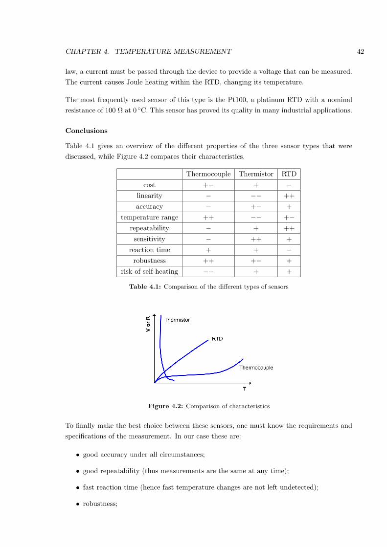
CHAPTER 4. TEMPERATURE MEASUREMENT 42
law, a current must be passed through the device to provide a voltage that can be measured.The current causes Joule heating within the RTD, changing its temperature.
The most frequently used sensor of this type is the Pt100, a platinum RTD with a nominalresistance of 100 Ω at 0 C. This sensor has proved its quality in many industrial applications.
Conclusions
Table 4.1 gives an overview of the different properties of the three sensor types that werediscussed, while Figure 4.2 compares their characteristics.
Thermocouple Thermistor RTD
cost +− + −linearity − −− ++
accuracy − +− +
temperature range ++ −− +−repeatability − + ++
sensitivity − ++ +
reaction time + + −robustness ++ +− +
risk of self-heating −− + +
Table 4.1: Comparison of the different types of sensors
Figure 4.2: Comparison of characteristics
To finally make the best choice between these sensors, one must know the requirements andspecifications of the measurement. In our case these are:
• good accuracy under all circumstances;
• good repeatability (thus measurements are the same at any time);
• fast reaction time (hence fast temperature changes are not left undetected);
• robustness;
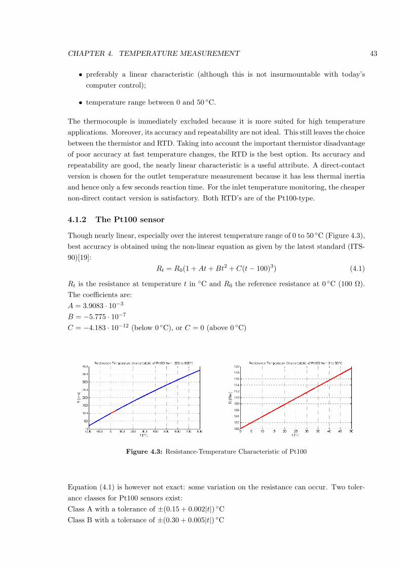
CHAPTER 4. TEMPERATURE MEASUREMENT 43
• preferably a linear characteristic (although this is not insurmountable with today’scomputer control);
• temperature range between 0 and 50 C.
The thermocouple is immediately excluded because it is more suited for high temperatureapplications. Moreover, its accuracy and repeatability are not ideal. This still leaves the choicebetween the thermistor and RTD. Taking into account the important thermistor disadvantageof poor accuracy at fast temperature changes, the RTD is the best option. Its accuracy andrepeatability are good, the nearly linear characteristic is a useful attribute. A direct-contactversion is chosen for the outlet temperature measurement because it has less thermal inertiaand hence only a few seconds reaction time. For the inlet temperature monitoring, the cheapernon-direct contact version is satisfactory. Both RTD’s are of the Pt100-type.
4.1.2 The Pt100 sensor
Though nearly linear, especially over the interest temperature range of 0 to 50 C (Figure 4.3),best accuracy is obtained using the non-linear equation as given by the latest standard (ITS-90)[19]:
Rt = R0(1 + At + Bt2 + C(t− 100)3) (4.1)
Rt is the resistance at temperature t in C and R0 the reference resistance at 0 C (100 Ω).The coefficients are:A = 3.9083 · 10−3
B = −5.775 · 10−7
C = −4.183 · 10−12 (below 0 C), or C = 0 (above 0 C)
Figure 4.3: Resistance-Temperature Characteristic of Pt100
Equation (4.1) is however not exact: some variation on the resistance can occur. Two toler-ance classes for Pt100 sensors exist:Class A with a tolerance of ±(0.15 + 0.002|t|) CClass B with a tolerance of ±(0.30 + 0.005|t|) C
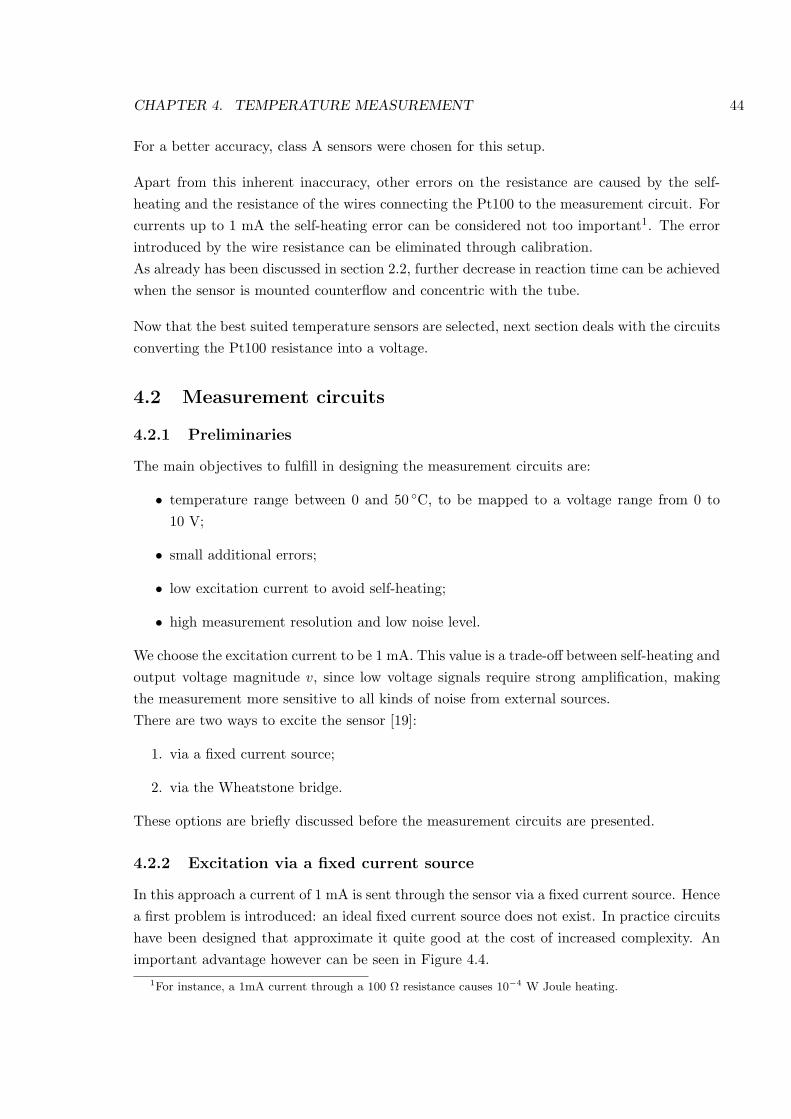
CHAPTER 4. TEMPERATURE MEASUREMENT 44
For a better accuracy, class A sensors were chosen for this setup.
Apart from this inherent inaccuracy, other errors on the resistance are caused by the self-heating and the resistance of the wires connecting the Pt100 to the measurement circuit. Forcurrents up to 1 mA the self-heating error can be considered not too important1. The errorintroduced by the wire resistance can be eliminated through calibration.As already has been discussed in section 2.2, further decrease in reaction time can be achievedwhen the sensor is mounted counterflow and concentric with the tube.
Now that the best suited temperature sensors are selected, next section deals with the circuitsconverting the Pt100 resistance into a voltage.
4.2 Measurement circuits
4.2.1 Preliminaries
The main objectives to fulfill in designing the measurement circuits are:
• temperature range between 0 and 50 C, to be mapped to a voltage range from 0 to10 V;
• small additional errors;
• low excitation current to avoid self-heating;
• high measurement resolution and low noise level.
We choose the excitation current to be 1 mA. This value is a trade-off between self-heating andoutput voltage magnitude v, since low voltage signals require strong amplification, makingthe measurement more sensitive to all kinds of noise from external sources.There are two ways to excite the sensor [19]:
1. via a fixed current source;
2. via the Wheatstone bridge.
These options are briefly discussed before the measurement circuits are presented.
4.2.2 Excitation via a fixed current source
In this approach a current of 1 mA is sent through the sensor via a fixed current source. Hencea first problem is introduced: an ideal fixed current source does not exist. In practice circuitshave been designed that approximate it quite good at the cost of increased complexity. Animportant advantage however can be seen in Figure 4.4.
1For instance, a 1mA current through a 100 Ω resistance causes 10−4 W Joule heating.
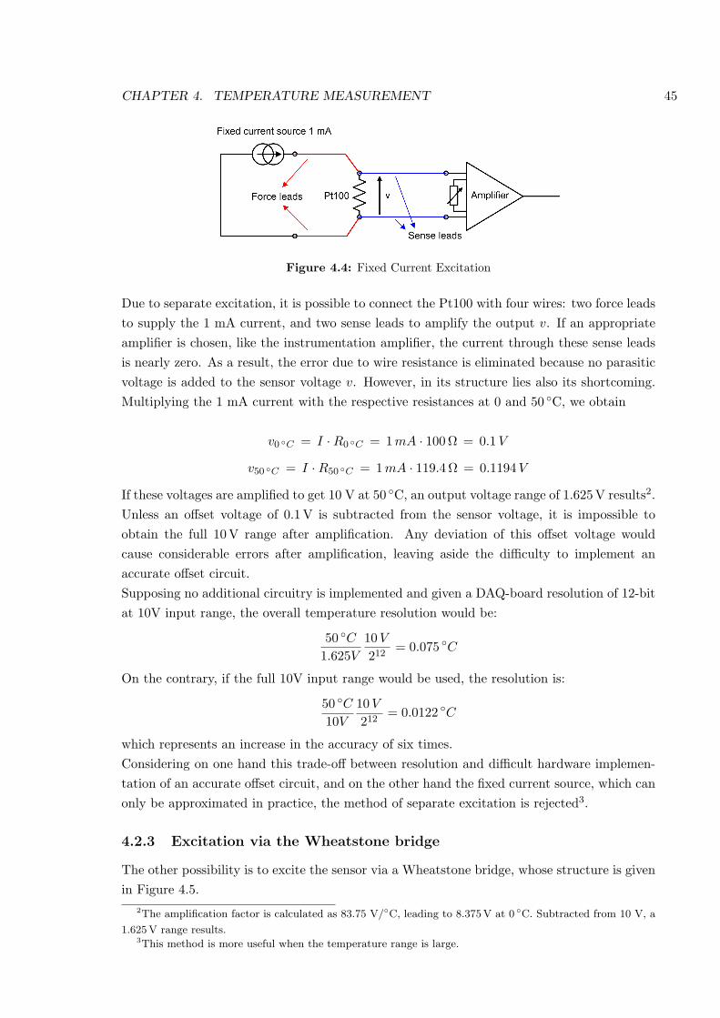
CHAPTER 4. TEMPERATURE MEASUREMENT 45
Figure 4.4: Fixed Current Excitation
Due to separate excitation, it is possible to connect the Pt100 with four wires: two force leadsto supply the 1 mA current, and two sense leads to amplify the output v. If an appropriateamplifier is chosen, like the instrumentation amplifier, the current through these sense leadsis nearly zero. As a result, the error due to wire resistance is eliminated because no parasiticvoltage is added to the sensor voltage v. However, in its structure lies also its shortcoming.Multiplying the 1 mA current with the respective resistances at 0 and 50 C, we obtain
v0 C = I ·R0 C = 1 mA · 100 Ω = 0.1 V
v50 C = I ·R50 C = 1 mA · 119.4 Ω = 0.1194 V
If these voltages are amplified to get 10 V at 50 C, an output voltage range of 1.625 V results2.Unless an offset voltage of 0.1V is subtracted from the sensor voltage, it is impossible toobtain the full 10 V range after amplification. Any deviation of this offset voltage wouldcause considerable errors after amplification, leaving aside the difficulty to implement anaccurate offset circuit.Supposing no additional circuitry is implemented and given a DAQ-board resolution of 12-bitat 10V input range, the overall temperature resolution would be:
50 C
1.625V
10 V
212= 0.075 C
On the contrary, if the full 10V input range would be used, the resolution is:
50 C
10V
10 V
212= 0.0122 C
which represents an increase in the accuracy of six times.Considering on one hand this trade-off between resolution and difficult hardware implemen-tation of an accurate offset circuit, and on the other hand the fixed current source, which canonly be approximated in practice, the method of separate excitation is rejected3.
4.2.3 Excitation via the Wheatstone bridge
The other possibility is to excite the sensor via a Wheatstone bridge, whose structure is givenin Figure 4.5.
2The amplification factor is calculated as 83.75 V/C, leading to 8.375V at 0 C. Subtracted from 10 V, a
1.625 V range results.3This method is more useful when the temperature range is large.
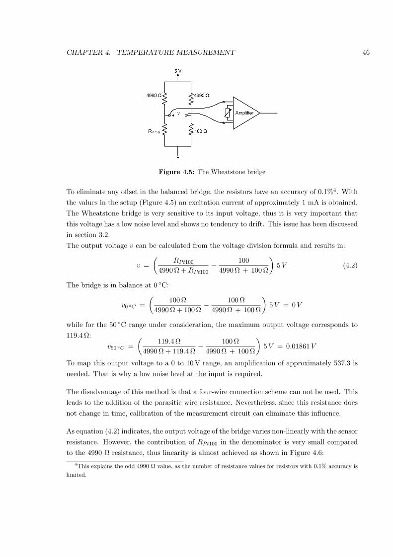
CHAPTER 4. TEMPERATURE MEASUREMENT 46
Figure 4.5: The Wheatstone bridge
To eliminate any offset in the balanced bridge, the resistors have an accuracy of 0.1%4. Withthe values in the setup (Figure 4.5) an excitation current of approximately 1 mA is obtained.The Wheatstone bridge is very sensitive to its input voltage, thus it is very important thatthis voltage has a low noise level and shows no tendency to drift. This issue has been discussedin section 3.2.The output voltage v can be calculated from the voltage division formula and results in:
v =(
RPt100
4990 Ω + RPt100− 100
4990 Ω + 100 Ω
)5 V (4.2)
The bridge is in balance at 0 C:
v0 C =(
100 Ω4990 Ω + 100 Ω
− 100 Ω4990 Ω + 100Ω
)5 V = 0 V
while for the 50 C range under consideration, the maximum output voltage corresponds to119.4 Ω:
v50 C =(
119.4 Ω4990 Ω + 119.4 Ω
− 100 Ω4990 Ω + 100Ω
)5 V = 0.01861 V
To map this output voltage to a 0 to 10V range, an amplification of approximately 537.3 isneeded. That is why a low noise level at the input is required.
The disadvantage of this method is that a four-wire connection scheme can not be used. Thisleads to the addition of the parasitic wire resistance. Nevertheless, since this resistance doesnot change in time, calibration of the measurement circuit can eliminate this influence.
As equation (4.2) indicates, the output voltage of the bridge varies non-linearly with the sensorresistance. However, the contribution of RPt100 in the denominator is very small comparedto the 4990 Ω resistance, thus linearity is almost achieved as shown in Figure 4.6:
4This explains the odd 4990 Ω value, as the number of resistance values for resistors with 0.1% accuracy is
limited.
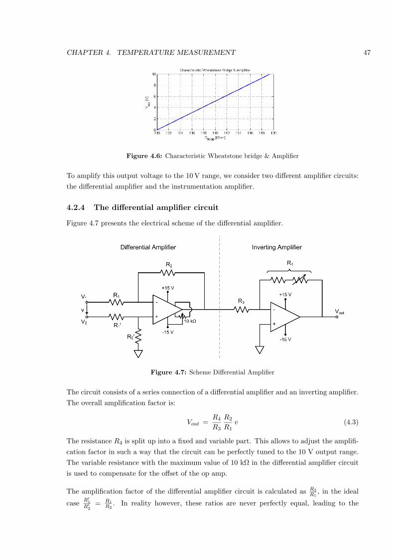
CHAPTER 4. TEMPERATURE MEASUREMENT 47
Figure 4.6: Characteristic Wheatstone bridge & Amplifier
To amplify this output voltage to the 10 V range, we consider two different amplifier circuits:the differential amplifier and the instrumentation amplifier.
4.2.4 The differential amplifier circuit
Figure 4.7 presents the electrical scheme of the differential amplifier.
Figure 4.7: Scheme Differential Amplifier
The circuit consists of a series connection of a differential amplifier and an inverting amplifier.The overall amplification factor is:
Vout =R4
R3
R2
R1v (4.3)
The resistance R4 is split up into a fixed and variable part. This allows to adjust the amplifi-cation factor in such a way that the circuit can be perfectly tuned to the 10 V output range.The variable resistance with the maximum value of 10 kΩ in the differential amplifier circuitis used to compensate for the offset of the op amp.
The amplification factor of the differential amplifier circuit is calculated as R2R1
, in the ideal
case R′1
R′2
= R1R2
. In reality however, these ratios are never perfectly equal, leading to the
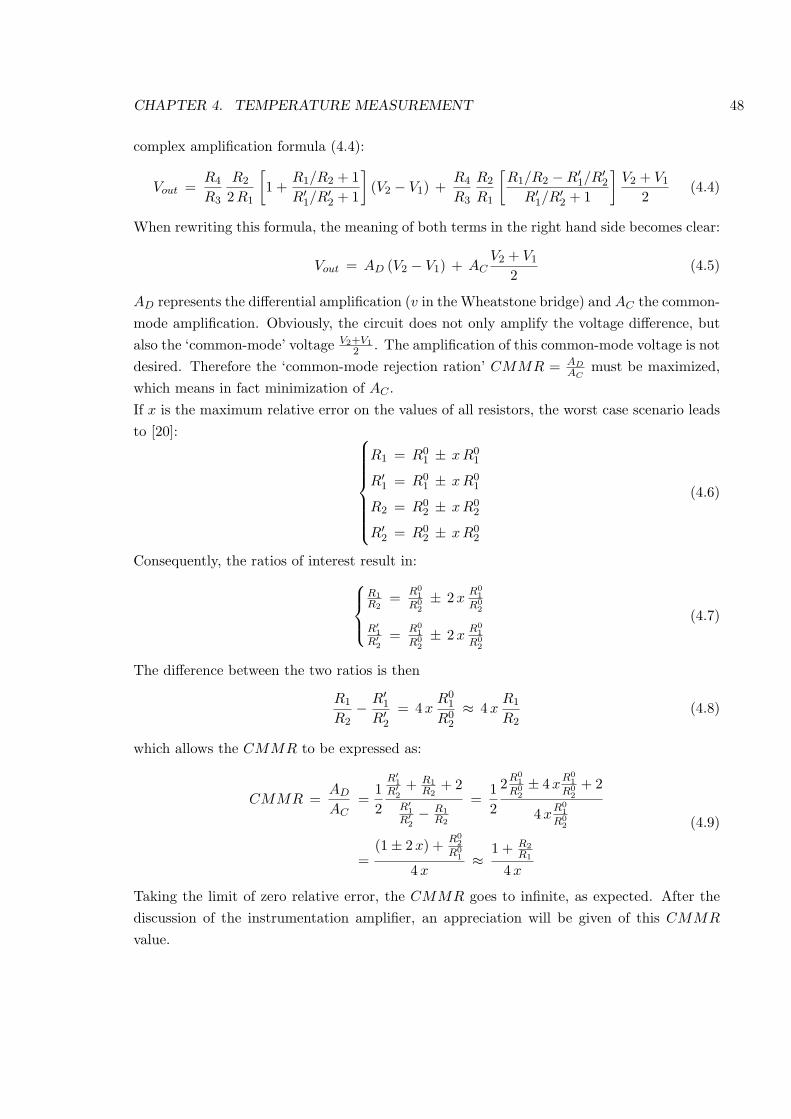
CHAPTER 4. TEMPERATURE MEASUREMENT 48
complex amplification formula (4.4):
Vout =R4
R3
R2
2 R1
[1 +
R1/R2 + 1R′
1/R′2 + 1
](V2 − V1) +
R4
R3
R2
R1
[R1/R2 −R′
1/R′2
R′1/R′
2 + 1
]V2 + V1
2(4.4)
When rewriting this formula, the meaning of both terms in the right hand side becomes clear:
Vout = AD (V2 − V1) + ACV2 + V1
2(4.5)
AD represents the differential amplification (v in the Wheatstone bridge) and AC the common-mode amplification. Obviously, the circuit does not only amplify the voltage difference, butalso the ‘common-mode’ voltage V2+V1
2 . The amplification of this common-mode voltage is notdesired. Therefore the ‘common-mode rejection ration’ CMMR = AD
ACmust be maximized,
which means in fact minimization of AC .If x is the maximum relative error on the values of all resistors, the worst case scenario leadsto [20]:
R1 = R01 ± xR0
1
R′1 = R0
1 ± xR01
R2 = R02 ± xR0
2
R′2 = R0
2 ± xR02
(4.6)
Consequently, the ratios of interest result in:R1R2
= R01
R02± 2 x
R01
R02
R′1
R′2
= R01
R02± 2 x
R01
R02
(4.7)
The difference between the two ratios is then
R1
R2− R′
1
R′2
= 4 xR0
1
R02
≈ 4 xR1
R2(4.8)
which allows the CMMR to be expressed as:
CMMR =AD
AC=
12
R′1
R′2
+ R1R2
+ 2R′
1R′
2− R1
R2
=12
2R01
R02± 4 x
R01
R02
+ 2
4 xR0
1
R02
=(1± 2 x) + R0
2
R01
4 x≈
1 + R2R1
4 x
(4.9)
Taking the limit of zero relative error, the CMMR goes to infinite, as expected. After thediscussion of the instrumentation amplifier, an appreciation will be given of this CMMR
value.
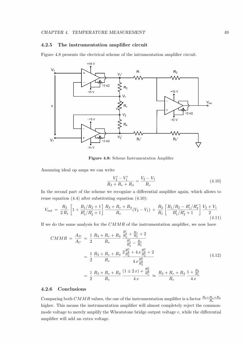
CHAPTER 4. TEMPERATURE MEASUREMENT 49
4.2.5 The instrumentation amplifier circuit
Figure 4.8 presents the electrical scheme of the intrumentation amplifier circuit.
Figure 4.8: Scheme Instrumentation Amplifier
Assuming ideal op amps we can write
V ′2 − V ′
1
R3 + Rv + R4=
V2 − V1
Rv(4.10)
In the second part of the scheme we recognize a differential amplifier again, which allows toreuse equation (4.4) after substituting equation (4.10):
Vout =R2
2 R1
[1 +
R1/R2 + 1R′
1/R′2 + 1
]R3 + Rv + R4
Rv(V2 − V1) +
R2
R1
[R1/R2 −R′
1/R′2
R′1/R′
2 + 1
]V2 + V1
2(4.11)
If we do the same analysis for the CMMR of the instrumentation amplifier, we now have
CMMR =AD
AC=
12
R3 + Rv + R4
Rv
R′1
R′2
+ R1R2
+ 2R′
1R′
2− R1
R2
=12
R3 + Rv + R4
Rv
2R01
R02
+ 4 xR0
1
R02
+ 2
4 xR0
1
R02
=12
R3 + Rv + R4
Rv
(1± 2 x) + R02
R01
4 x≈ R3 + Rv + R4
Rv
1 + R2R1
4 x
(4.12)
4.2.6 Conclusions
Comparing both CMMR values, the one of the instrumentation amplifier is a factor R3+Rv+R4Rv
higher. This means the instrumentation amplifier will almost completely reject the common-mode voltage to merely amplify the Wheatstone bridge output voltage v, while the differentialamplifier will add an extra voltage.
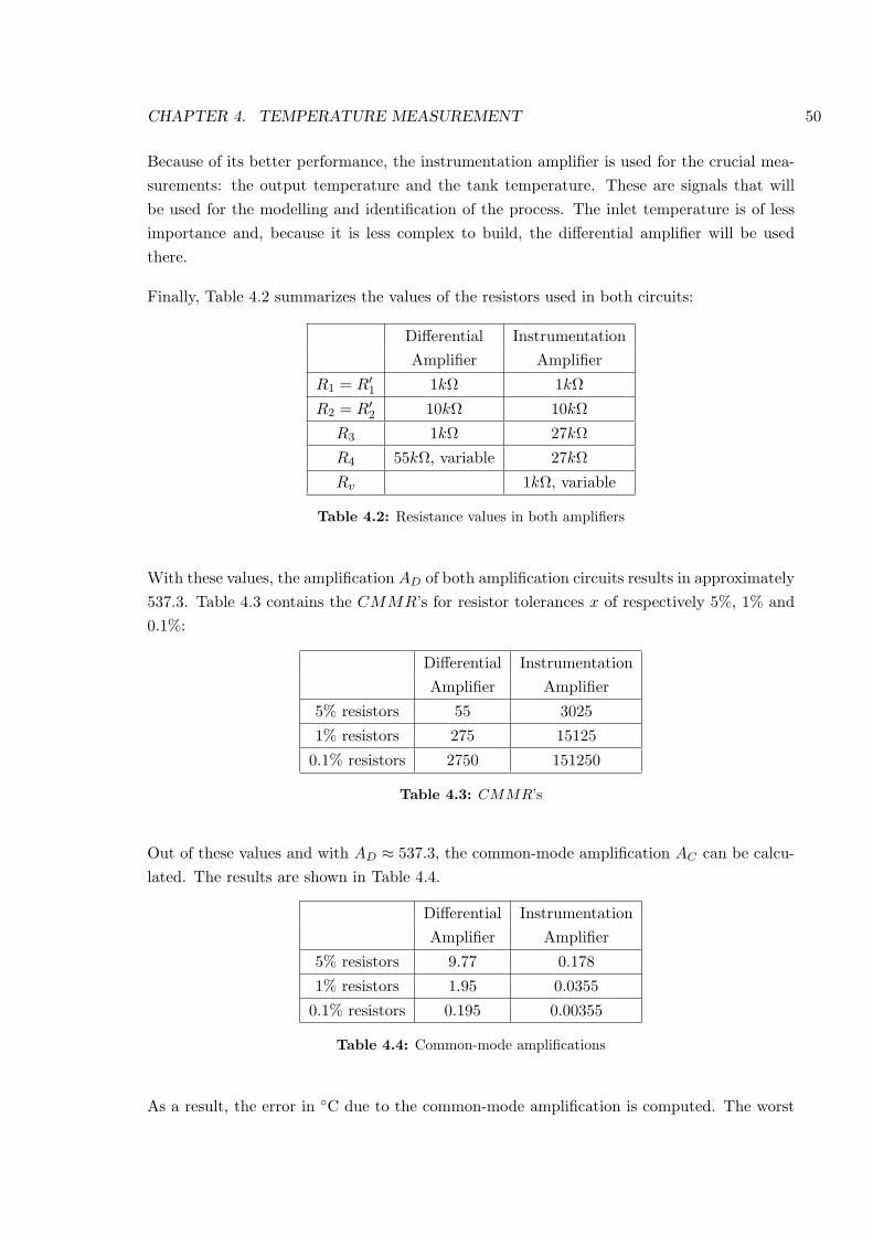
CHAPTER 4. TEMPERATURE MEASUREMENT 50
Because of its better performance, the instrumentation amplifier is used for the crucial mea-surements: the output temperature and the tank temperature. These are signals that willbe used for the modelling and identification of the process. The inlet temperature is of lessimportance and, because it is less complex to build, the differential amplifier will be usedthere.
Finally, Table 4.2 summarizes the values of the resistors used in both circuits:
Differential InstrumentationAmplifier Amplifier
R1 = R′1 1kΩ 1kΩ
R2 = R′2 10kΩ 10kΩ
R3 1kΩ 27kΩ
R4 55kΩ, variable 27kΩ
Rv 1kΩ, variable
Table 4.2: Resistance values in both amplifiers
With these values, the amplification AD of both amplification circuits results in approximately537.3. Table 4.3 contains the CMMR’s for resistor tolerances x of respectively 5%, 1% and0.1%:
Differential InstrumentationAmplifier Amplifier
5% resistors 55 3025
1% resistors 275 15125
0.1% resistors 2750 151250
Table 4.3: CMMR’s
Out of these values and with AD ≈ 537.3, the common-mode amplification AC can be calcu-lated. The results are shown in Table 4.4.
Differential InstrumentationAmplifier Amplifier
5% resistors 9.77 0.178
1% resistors 1.95 0.0355
0.1% resistors 0.195 0.00355
Table 4.4: Common-mode amplifications
As a result, the error in C due to the common-mode amplification is computed. The worst
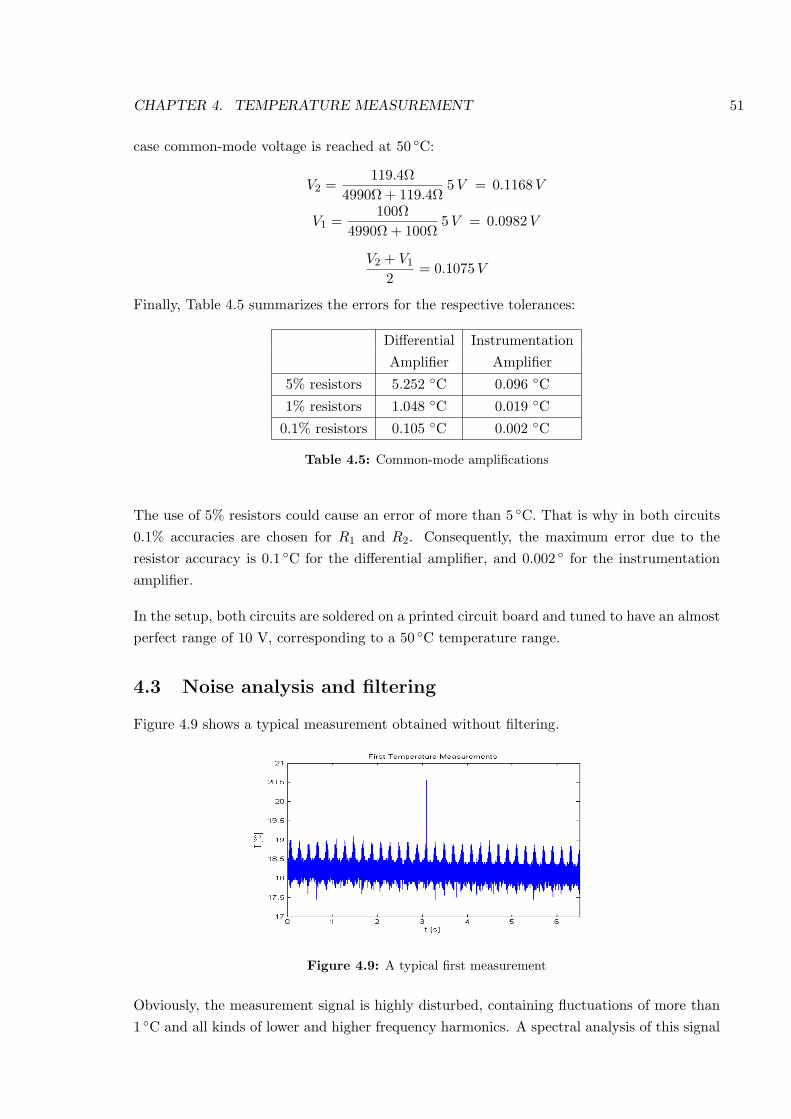
CHAPTER 4. TEMPERATURE MEASUREMENT 51
case common-mode voltage is reached at 50 C:
V2 =119.4Ω
4990Ω + 119.4Ω5 V = 0.1168 V
V1 =100Ω
4990Ω + 100Ω5 V = 0.0982 V
V2 + V1
2= 0.1075 V
Finally, Table 4.5 summarizes the errors for the respective tolerances:
Differential InstrumentationAmplifier Amplifier
5% resistors 5.252 C 0.096 C
1% resistors 1.048 C 0.019 C
0.1% resistors 0.105 C 0.002 C
Table 4.5: Common-mode amplifications
The use of 5% resistors could cause an error of more than 5 C. That is why in both circuits0.1% accuracies are chosen for R1 and R2. Consequently, the maximum error due to theresistor accuracy is 0.1 C for the differential amplifier, and 0.002 for the instrumentationamplifier.
In the setup, both circuits are soldered on a printed circuit board and tuned to have an almostperfect range of 10 V, corresponding to a 50 C temperature range.
4.3 Noise analysis and filtering
Figure 4.9 shows a typical measurement obtained without filtering.
Figure 4.9: A typical first measurement
Obviously, the measurement signal is highly disturbed, containing fluctuations of more than1 C and all kinds of lower and higher frequency harmonics. A spectral analysis of this signal
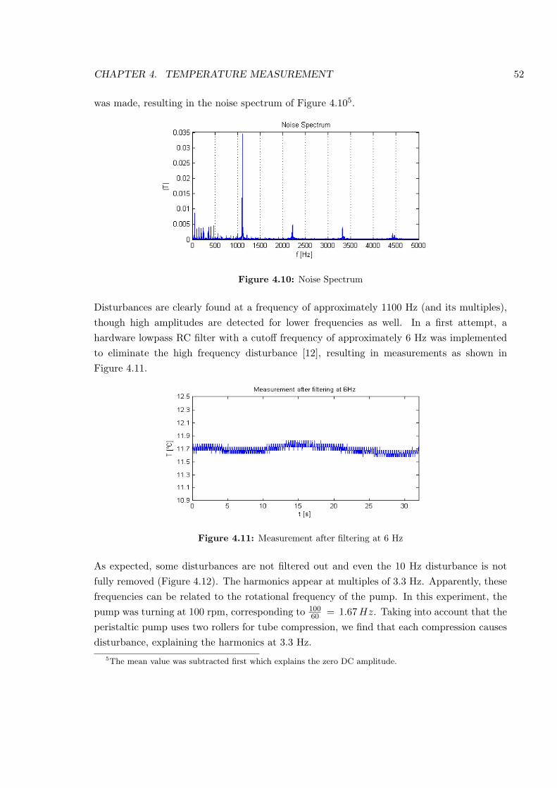
CHAPTER 4. TEMPERATURE MEASUREMENT 52
was made, resulting in the noise spectrum of Figure 4.105.
Figure 4.10: Noise Spectrum
Disturbances are clearly found at a frequency of approximately 1100 Hz (and its multiples),though high amplitudes are detected for lower frequencies as well. In a first attempt, ahardware lowpass RC filter with a cutoff frequency of approximately 6 Hz was implementedto eliminate the high frequency disturbance [12], resulting in measurements as shown inFigure 4.11.
Figure 4.11: Measurement after filtering at 6 Hz
As expected, some disturbances are not filtered out and even the 10 Hz disturbance is notfully removed (Figure 4.12). The harmonics appear at multiples of 3.3 Hz. Apparently, thesefrequencies can be related to the rotational frequency of the pump. In this experiment, thepump was turning at 100 rpm, corresponding to 100
60 = 1.67 Hz. Taking into account that theperistaltic pump uses two rollers for tube compression, we find that each compression causesdisturbance, explaining the harmonics at 3.3 Hz.
5The mean value was subtracted first which explains the zero DC amplitude.
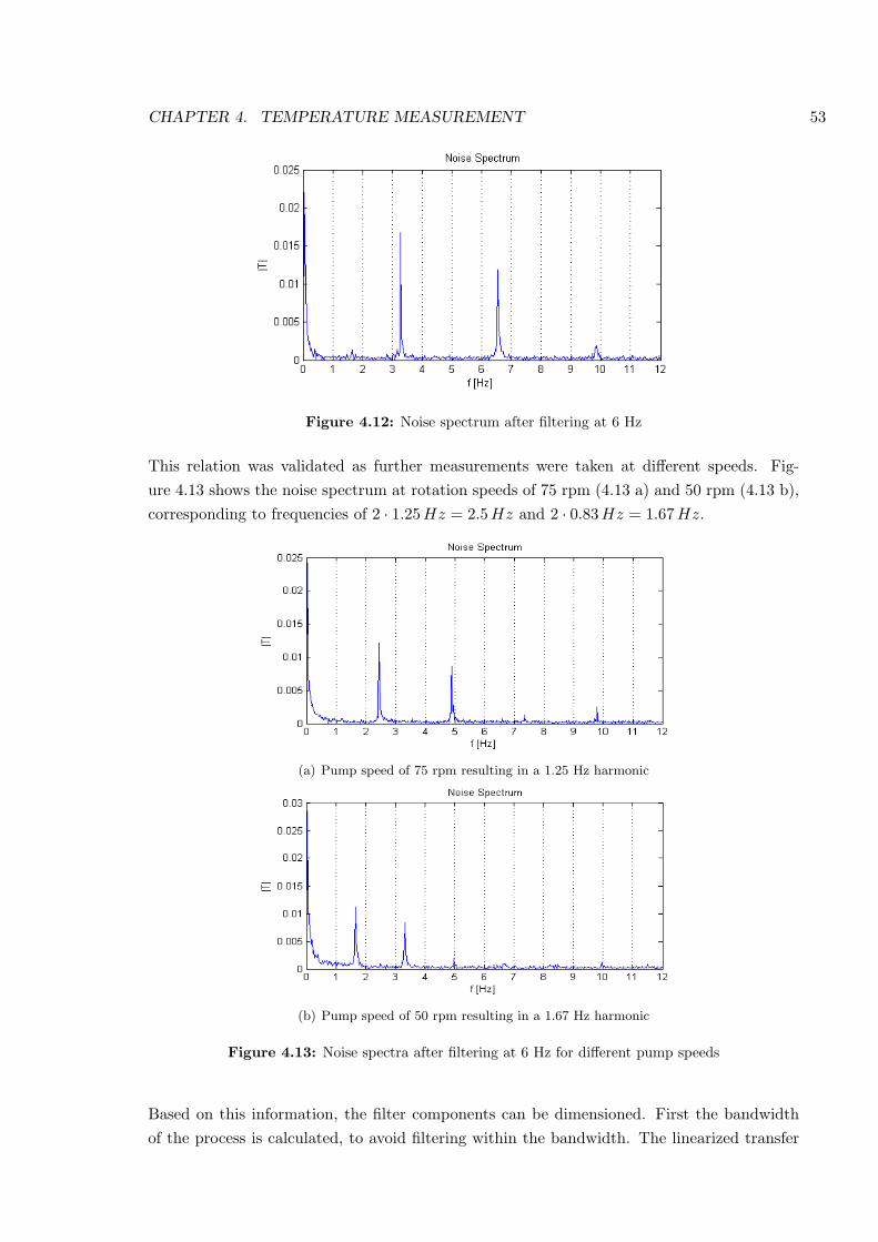
CHAPTER 4. TEMPERATURE MEASUREMENT 53
Figure 4.12: Noise spectrum after filtering at 6 Hz
This relation was validated as further measurements were taken at different speeds. Fig-ure 4.13 shows the noise spectrum at rotation speeds of 75 rpm (4.13 a) and 50 rpm (4.13 b),corresponding to frequencies of 2 · 1.25 Hz = 2.5 Hz and 2 · 0.83 Hz = 1.67 Hz.
(a) Pump speed of 75 rpm resulting in a 1.25 Hz harmonic
(b) Pump speed of 50 rpm resulting in a 1.67 Hz harmonic
Figure 4.13: Noise spectra after filtering at 6 Hz for different pump speeds
Based on this information, the filter components can be dimensioned. First the bandwidthof the process is calculated, to avoid filtering within the bandwidth. The linearized transfer
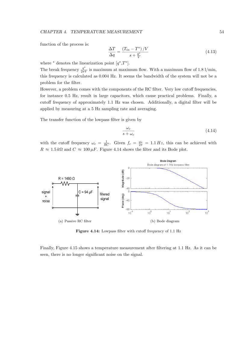
CHAPTER 4. TEMPERATURE MEASUREMENT 54
function of the process is:∆T
∆q=
(Tin − T ∗) /V
s + q∗
V
(4.13)
where ∗ denotes the linearization point [q∗,T ∗].The break frequency q∗
2πV is maximum at maximum flow. With a maximum flow of 1.8 l/min,this frequency is calculated as 0.004 Hz. It seems the bandwidth of the system will not be aproblem for the filter.However, a problem comes with the components of the RC filter. Very low cutoff frequencies,for instance 0.5 Hz, result in large capacitors, which cause practical problems. Finally, acutoff frequency of approximately 1.1 Hz was chosen. Additionally, a digital filter will beapplied by measuring at a 5 Hz sampling rate and averaging.
The transfer function of the lowpass filter is given by
ωc
s + ωc(4.14)
with the cutoff frequency ωc = 1RC . Given fc = ωc
2π = 1.1 Hz, this can be achieved withR ≈ 1.5 kΩ and C ≈ 100 µF . Figure 4.14 shows the filter and its Bode plot.
(a) Passive RC filter (b) Bode diagram
Figure 4.14: Lowpass filter with cutoff frequency of 1.1 Hz
Finally, Figure 4.15 shows a temperature measurement after filtering at 1.1 Hz. As it can beseen, there is no longer significant noise on the signal.
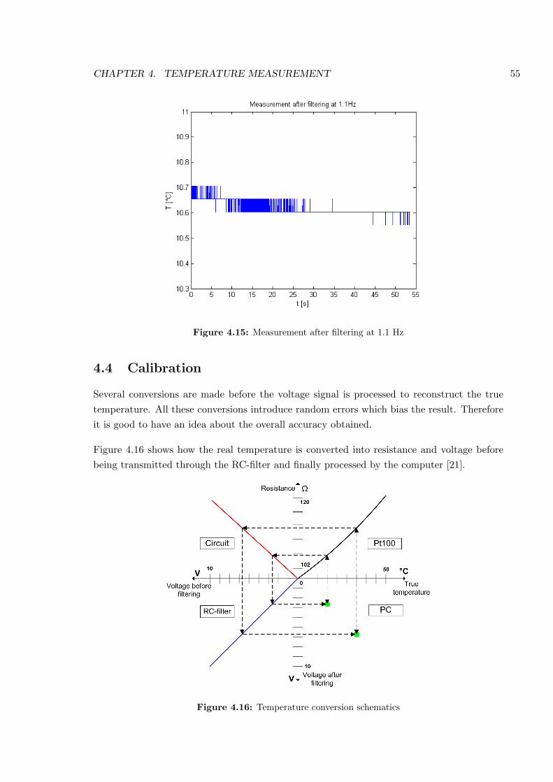
CHAPTER 4. TEMPERATURE MEASUREMENT 55
Figure 4.15: Measurement after filtering at 1.1 Hz
4.4 Calibration
Several conversions are made before the voltage signal is processed to reconstruct the truetemperature. All these conversions introduce random errors which bias the result. Thereforeit is good to have an idea about the overall accuracy obtained.
Figure 4.16 shows how the real temperature is converted into resistance and voltage beforebeing transmitted through the RC-filter and finally processed by the computer [21].
Figure 4.16: Temperature conversion schematics
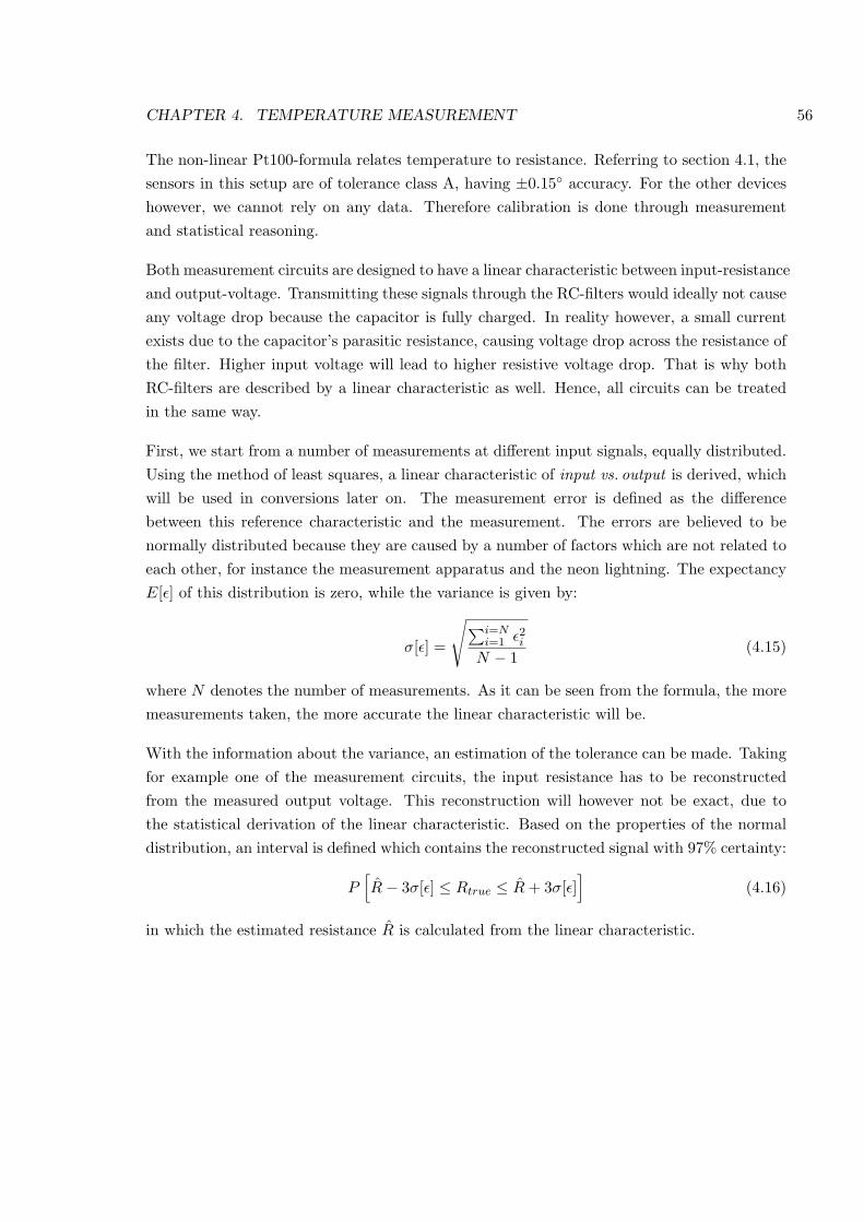
CHAPTER 4. TEMPERATURE MEASUREMENT 56
The non-linear Pt100-formula relates temperature to resistance. Referring to section 4.1, thesensors in this setup are of tolerance class A, having ±0.15 accuracy. For the other deviceshowever, we cannot rely on any data. Therefore calibration is done through measurementand statistical reasoning.
Both measurement circuits are designed to have a linear characteristic between input-resistanceand output-voltage. Transmitting these signals through the RC-filters would ideally not causeany voltage drop because the capacitor is fully charged. In reality however, a small currentexists due to the capacitor’s parasitic resistance, causing voltage drop across the resistance ofthe filter. Higher input voltage will lead to higher resistive voltage drop. That is why bothRC-filters are described by a linear characteristic as well. Hence, all circuits can be treatedin the same way.
First, we start from a number of measurements at different input signals, equally distributed.Using the method of least squares, a linear characteristic of input vs. output is derived, whichwill be used in conversions later on. The measurement error is defined as the differencebetween this reference characteristic and the measurement. The errors are believed to benormally distributed because they are caused by a number of factors which are not related toeach other, for instance the measurement apparatus and the neon lightning. The expectancyE[ε] of this distribution is zero, while the variance is given by:
σ[ε] =
√∑i=Ni=1 ε2i
N − 1(4.15)
where N denotes the number of measurements. As it can be seen from the formula, the moremeasurements taken, the more accurate the linear characteristic will be.
With the information about the variance, an estimation of the tolerance can be made. Takingfor example one of the measurement circuits, the input resistance has to be reconstructedfrom the measured output voltage. This reconstruction will however not be exact, due tothe statistical derivation of the linear characteristic. Based on the properties of the normaldistribution, an interval is defined which contains the reconstructed signal with 97% certainty:
P[R− 3σ[ε] ≤ Rtrue ≤ R + 3σ[ε]
](4.16)
in which the estimated resistance R is calculated from the linear characteristic.
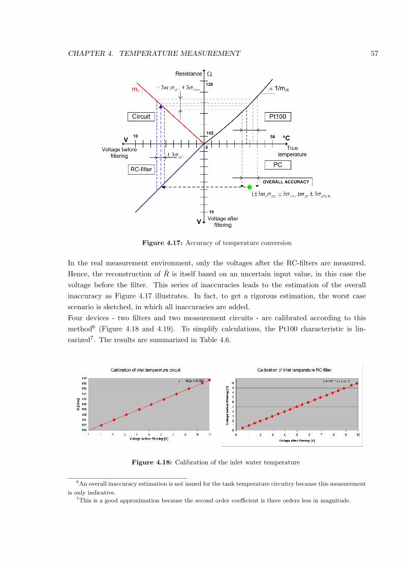
CHAPTER 4. TEMPERATURE MEASUREMENT 57
Figure 4.17: Accuracy of temperature conversion
In the real measurement environment, only the voltages after the RC-filters are measured.Hence, the reconstruction of R is itself based on an uncertain input value, in this case thevoltage before the filter. This series of inaccuracies leads to the estimation of the overallinaccuracy as Figure 4.17 illustrates. In fact, to get a rigorous estimation, the worst casescenario is sketched, in which all inaccuracies are added.Four devices - two filters and two measurement circuits - are calibrated according to thismethod6 (Figure 4.18 and 4.19). To simplify calculations, the Pt100 characteristic is lin-earized7. The results are summarized in Table 4.6.
Figure 4.18: Calibration of the inlet water temperature
6An overall inaccuracy estimation is not issued for the tank temperature circuitry because this measurement
is only indicative.7This is a good approximation because the second order coefficient is three orders less in magnitude.
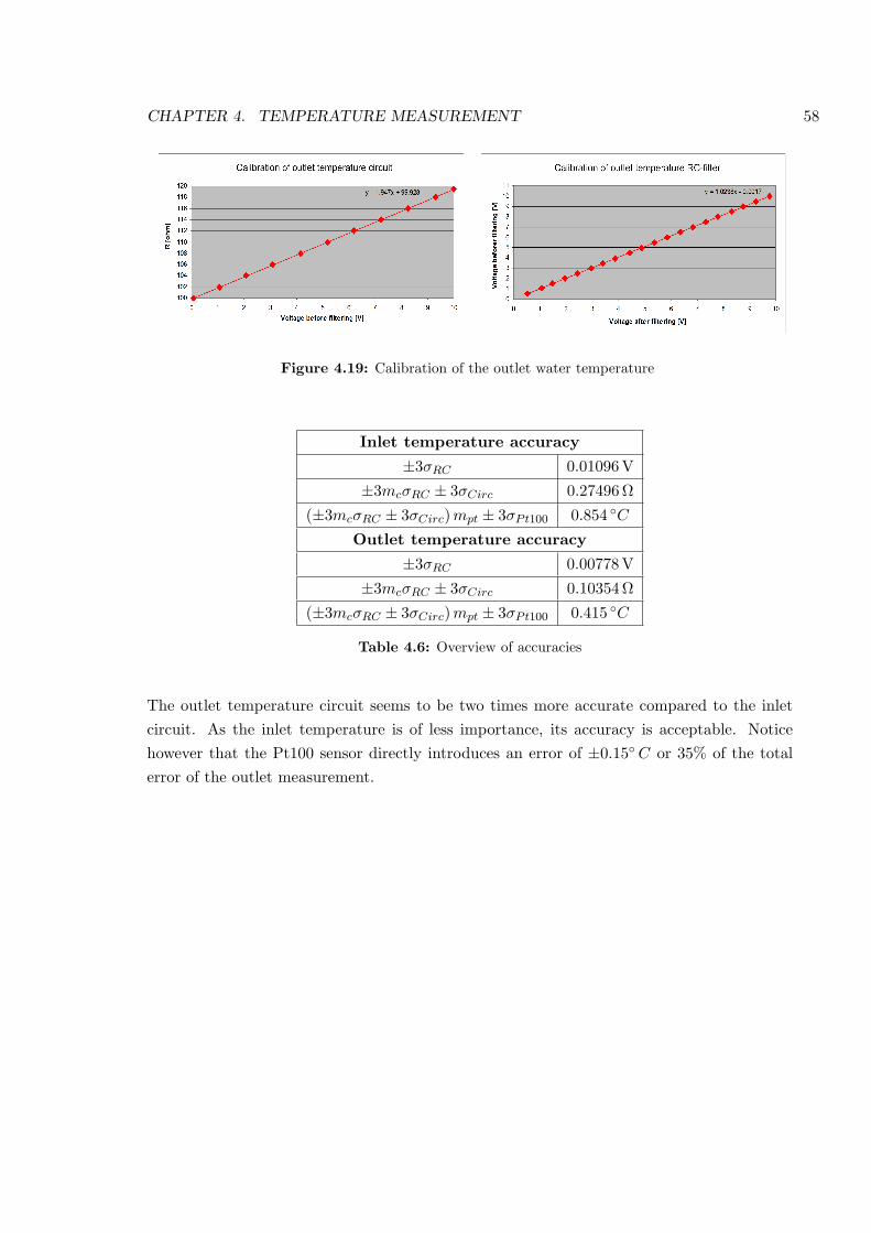
CHAPTER 4. TEMPERATURE MEASUREMENT 58
Figure 4.19: Calibration of the outlet water temperature
Inlet temperature accuracy
±3σRC 0.01096 V
±3mcσRC ± 3σCirc 0.27496 Ω
(±3mcσRC ± 3σCirc) mpt ± 3σPt100 0.854 C
Outlet temperature accuracy
±3σRC 0.00778 V
±3mcσRC ± 3σCirc 0.10354 Ω
(±3mcσRC ± 3σCirc) mpt ± 3σPt100 0.415 C
Table 4.6: Overview of accuracies
The outlet temperature circuit seems to be two times more accurate compared to the inletcircuit. As the inlet temperature is of less importance, its accuracy is acceptable. Noticehowever that the Pt100 sensor directly introduces an error of ±0.15 C or 35% of the totalerror of the outlet measurement.
Part II
Advanced Control
59
Chapter 5
Modelling and Identification
5.1 Preliminaries
In this chapter a model is derived for each part of the plant in a rigorous way. It is obvious thatthe success of this approach depends on the difficulty of the part under consideration. As aresult, we will sometimes be obliged to make some considerable simplifications or assumptionsin order to obtain a model that is useful for the predictive controller.
First the temperature dynamics of the water tank itself are discussed. These can be obtainedin a rather straightforward way using the energy balance. Next, the heat loss of the tank andthe outlet tube are investigated. Regarding these heat losses, mainly the results will be givenwhile the theory behind it will not be examined deeply, since this is of minor importance.Finally, a model of the outlet tube and the variable time delay will be derived. In the lastsection of this chapter, handling the identification, these theoretic results will be comparedto experimental data in order to check their accuracy and to see whether or not they needadjustment.
5.2 Water tank
A theoretical model of the water temperature dynamics can be derived departing from thefirst law for thermodynamic systems (energy balance, for more information on thermodynamicsystems, see [14]). As control volume the tank itself is considered (Figure 5.1). We recall thatin the tank there is a heater which is constantly turned on (thus no manipulation of the heatinput), while a mixer guarantees a uniform temperature in all the regions of the tank. Thewater level is kept constant by use of the mechanical float switch.
60
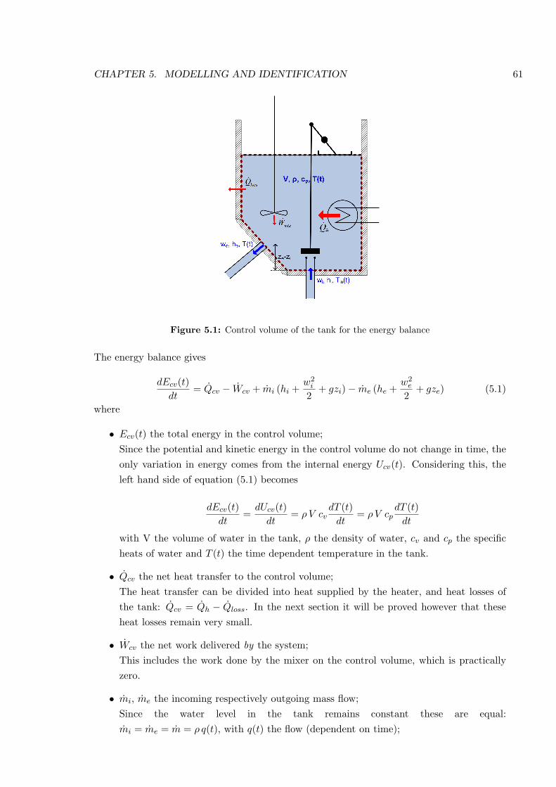
CHAPTER 5. MODELLING AND IDENTIFICATION 61
Figure 5.1: Control volume of the tank for the energy balance
The energy balance gives
dEcv(t)dt
= Qcv − Wcv + mi (hi +w2
i
2+ gzi)− me (he +
w2e
2+ gze) (5.1)
where
• Ecv(t) the total energy in the control volume;Since the potential and kinetic energy in the control volume do not change in time, theonly variation in energy comes from the internal energy Ucv(t). Considering this, theleft hand side of equation (5.1) becomes
dEcv(t)dt
=dUcv(t)
dt= ρ V cv
dT (t)dt
= ρ V cpdT (t)
dt
with V the volume of water in the tank, ρ the density of water, cv and cp the specificheats of water and T (t) the time dependent temperature in the tank.
• Qcv the net heat transfer to the control volume;The heat transfer can be divided into heat supplied by the heater, and heat losses ofthe tank: Qcv = Qh − Qloss. In the next section it will be proved however that theseheat losses remain very small.
• Wcv the net work delivered by the system;This includes the work done by the mixer on the control volume, which is practicallyzero.
• mi, me the incoming respectively outgoing mass flow;Since the water level in the tank remains constant these are equal:mi = me = m = ρ q(t), with q(t) the flow (dependent on time);
CHAPTER 5. MODELLING AND IDENTIFICATION 62
• hi, he the enthalpy of the incoming respectively outgoing water;This can be rewritten as
hi = cp Tin(t) en he = cp T (t)
• wi, we the velocity of the incoming respectively outgoing water;
• zi, ze the elevation of the inlet respectively outlet tube.
With the results described above, equation (5.1) becomes
ρ V cpdT (t)
dt= Qh + ρ q(t)
[cp (Tin(t)− T (t)) +
w2i − w2
e
2+ g (zi − ze)
](5.2)
Since the difference in velocity and elevation are negligible compared to the term containingthe specific heat, this expression can be simplified to
VdT (t)
dt=
Qh
ρ cp+ q(t) (Tin(t)− T (t)) (5.3)
This non-linear first order differential equation describes the temperature dynamics of thewater in the tank.
Since we are dealing with computer control, it is necessary to discretize equation (5.3) withrespect to the sampling period Ts. An important remark is that ‘t’ is used again, howeverit denotes the discrete time index now, and not the continuous time. After discretizing withrespect to Ts, equation (5.3) becomes
V
(T (t)− T (t− 1)
Ts
)=
Qh
ρ cp+ q(t− 1) (Tin(t− 1)− T (t− 1)) (5.4)
A few manipulations of equation (5.4) result in:
T (t)− T (t− 1) =Qh Ts
ρ V cp+
q(t− 1) Ts
V(Tin(t− 1)− T (t− 1)) (5.5)
T (t) = T (t− 1) +Ts
V
[Qh
ρ cp+ q(t− 1) (Tin(t− 1)− T (t− 1))
](5.6)
This expression represents the discrete time model of the water tank and will be validatedagainst experimental data.
5.3 Heat loss
5.3.1 Of the tank
The following heat losses should be considered [22],[23]:
• conduction through the walls of the tank;
• natural convection at the side and bottom of the tank walls, and at the water surface.
CHAPTER 5. MODELLING AND IDENTIFICATION 63
For simplicity we will consider the tank to have a rectangular shape. Note that this will nothave an important effect on the result. We will assume a worst case scenario of 40 C watertemperature, which will be approximately the maximum temperature for the system. Thetemperature of the surroundings is supposed to be 18 C. For each type of heat transfer wewill calculate the corresponding thermal resistance.
Conduction
The thermal resistance for conductive heat transfer through a straight wall is given by
Rconduction =∆x
k A(5.7)
with ∆x the thickness and A the area of the wall. For the tank, the walls are made of 5 mmthick plexiglass (PMMA) which has a thermal conductivity k of 0.18 W
m K . Each side wall hasan area of 0.0136 m2 resulting in a thermal resistance of:
Rcond,sidewall = 2.04K
W
For the floor wall (area 0.01 m2) we obtain:
Rcond,floor = 2.78K
W
Convection
The thermal resistance for convective heat transfer at a straight wall is given by
Rconvection =1
h A(5.8)
with h the convective heat coefficient. This parameter is calculated out of semi-empiric for-mulas that can be found in specialized literature [22]. Here, only the results are given:
Natural convection at a vertical wall: h = 5.91 Wm2 K
Natural convection at the bottom: h = 2.55 Wm2 K
Natural convection at the water surface: h = 5.70 Wm2 K
With these results we calculate the corresponding thermal resistances:
Rconv,sidewall = 12.43K
W
Rconv,floor = 39.23K
W
Rconv,surface = 17.55K
W
CHAPTER 5. MODELLING AND IDENTIFICATION 64
Total Heat loss
Once we have all thermal resistances, the respective heat losses can be calculated:
Qsidewall =Twater − Tsurrounding
Rcond,sidewall + Rconv,sidewall= 1.38 W
Qfloor =Twater − Tsurrounding
Rcond,floor + Rconv,floor= 0.48 W
Qsurface =Twater − Tsurrounding
Rconv,surface= 1.14 W
Hence, the total heat loss is obtained:
Qtotal = 4Qsidewall + Qfloor + Qsurface = 7.14 W
Although in this calculation heat loss due to radiation and evaporation are not taken intoaccount, it is clear that the heat loss will be small compared to the heat input of 1100 W.
5.3.2 In the tube
Heat loss without insulation of the tube
Here we identify conduction through and natural convection at the wall of the tube. Thetube is made of PVC, which has a thermal conductivity k of 0.15 W
m K . It is 9.5 m long, hasan inner diameter of 12 mm and a wall thickness of 2 mm. In all these calculations we willconsider the system in steady state, meaning a constant water temperature in the tank anda corresponding constant outflow q.
The thermal resistance for conduction through a circular tube is
Rconduction =ln(ro/ri)
2πkL(5.9)
with ro and ri the outer and inner radius of the tube, and L its length. Substituting the realvalues we obtain
Rconduction = 0.032K
W
After a number of calculations involving dimensionless units like Nusselt and Prandtl, theconvective heat coefficient is: h = 20.96 W
m2 K. Now, the thermal resistance for the convective
heat transfer can be estimated:
Rconvection =1
h 2πroL(5.10)
which results inRconvection = 0.10
K
W(5.11)
The overall heat loss results in
Q =Twater,avg − Tsurrounding
Rconduction + Rconvection= 137 W
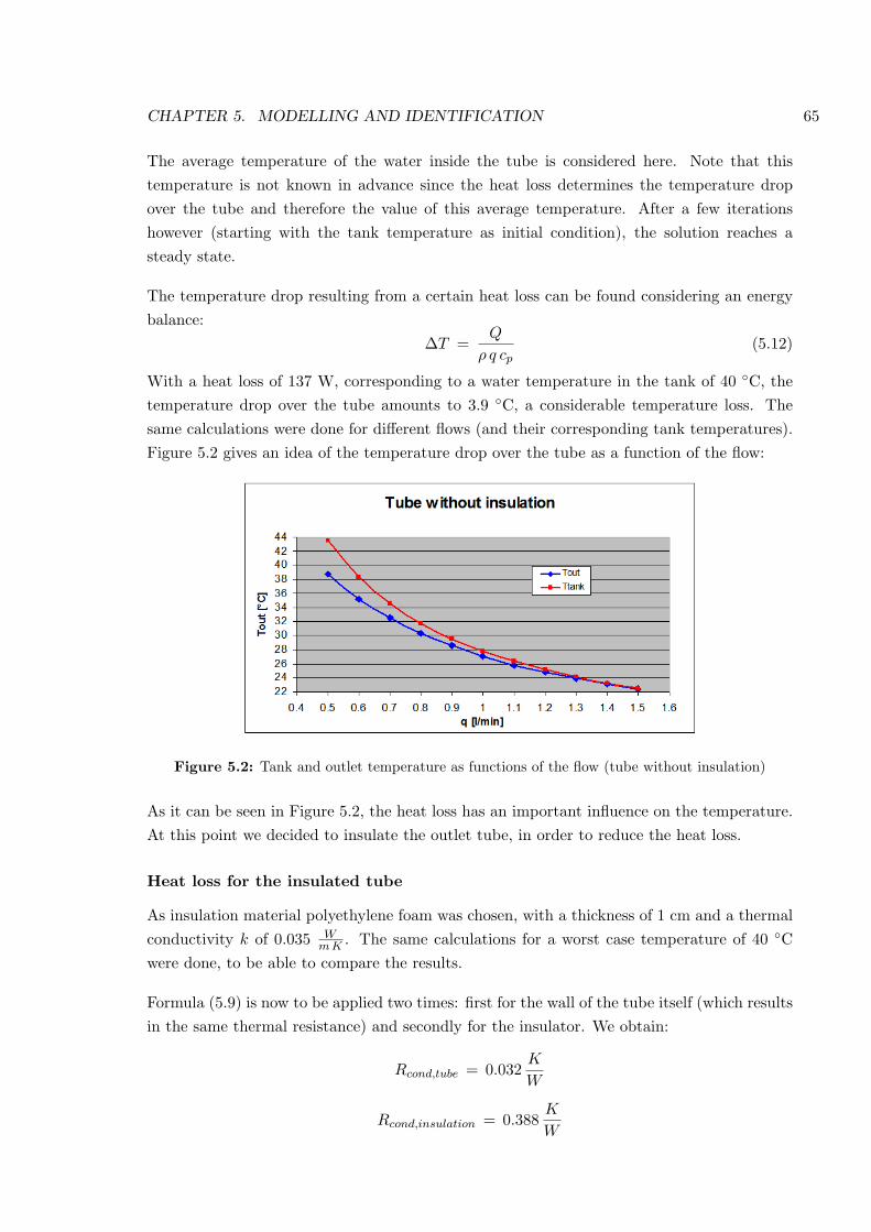
CHAPTER 5. MODELLING AND IDENTIFICATION 65
The average temperature of the water inside the tube is considered here. Note that thistemperature is not known in advance since the heat loss determines the temperature dropover the tube and therefore the value of this average temperature. After a few iterationshowever (starting with the tank temperature as initial condition), the solution reaches asteady state.
The temperature drop resulting from a certain heat loss can be found considering an energybalance:
∆T =Q
ρ q cp(5.12)
With a heat loss of 137 W, corresponding to a water temperature in the tank of 40 C, thetemperature drop over the tube amounts to 3.9 C, a considerable temperature loss. Thesame calculations were done for different flows (and their corresponding tank temperatures).Figure 5.2 gives an idea of the temperature drop over the tube as a function of the flow:
Figure 5.2: Tank and outlet temperature as functions of the flow (tube without insulation)
As it can be seen in Figure 5.2, the heat loss has an important influence on the temperature.At this point we decided to insulate the outlet tube, in order to reduce the heat loss.
Heat loss for the insulated tube
As insulation material polyethylene foam was chosen, with a thickness of 1 cm and a thermalconductivity k of 0.035 W
m K . The same calculations for a worst case temperature of 40 Cwere done, to be able to compare the results.
Formula (5.9) is now to be applied two times: first for the wall of the tube itself (which resultsin the same thermal resistance) and secondly for the insulator. We obtain:
Rcond,tube = 0.032K
W
Rcond,insulation = 0.388K
W
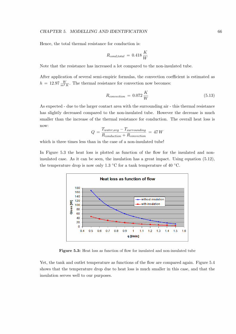
CHAPTER 5. MODELLING AND IDENTIFICATION 66
Hence, the total thermal resistance for conduction is:
Rcond,total = 0.418K
W
Note that the resistance has increased a lot compared to the non-insulated tube.
After application of several semi-empiric formulas, the convection coefficient is estimated ash = 12.97 W
m2 K. The thermal resistance for convection now becomes:
Rconvection = 0.072K
W(5.13)
As expected - due to the larger contact area with the surrounding air - this thermal resistancehas slightly decreased compared to the non-insulated tube. However the decrease is muchsmaller than the increase of the thermal resistance for conduction. The overall heat loss isnow:
Q =Twater,avg − Tsurrounding
Rconduction + Rconvection= 47 W
which is three times less than in the case of a non-insulated tube!
In Figure 5.3 the heat loss is plotted as function of the flow for the insulated and non-insulated case. As it can be seen, the insulation has a great impact. Using equation (5.12),the temperature drop is now only 1.3 C for a tank temperature of 40 C.
Figure 5.3: Heat loss as function of flow for insulated and non-insulated tube
Yet, the tank and outlet temperature as functions of the flow are compared again. Figure 5.4shows that the temperature drop due to heat loss is much smaller in this case, and that theinsulation serves well to our purposes.
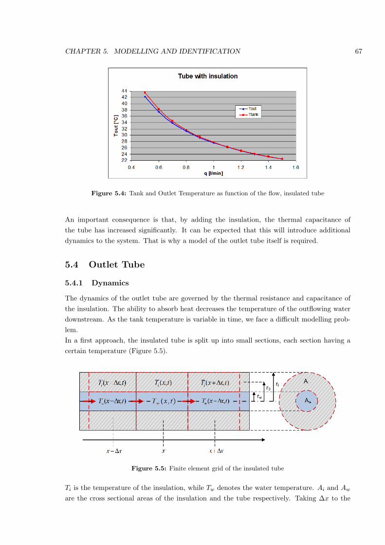
CHAPTER 5. MODELLING AND IDENTIFICATION 67
Figure 5.4: Tank and Outlet Temperature as function of the flow, insulated tube
An important consequence is that, by adding the insulation, the thermal capacitance ofthe tube has increased significantly. It can be expected that this will introduce additionaldynamics to the system. That is why a model of the outlet tube itself is required.
5.4 Outlet Tube
5.4.1 Dynamics
The dynamics of the outlet tube are governed by the thermal resistance and capacitance ofthe insulation. The ability to absorb heat decreases the temperature of the outflowing waterdownstream. As the tank temperature is variable in time, we face a difficult modelling prob-lem.In a first approach, the insulated tube is split up into small sections, each section having acertain temperature (Figure 5.5).
Figure 5.5: Finite element grid of the insulated tube
Ti is the temperature of the insulation, while Tw denotes the water temperature. Ai and Aw
are the cross sectional areas of the insulation and the tube respectively. Taking ∆x to the
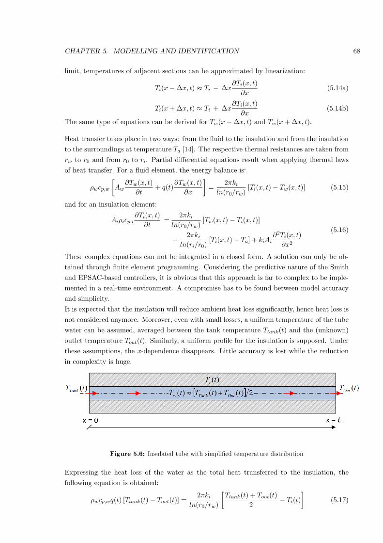
CHAPTER 5. MODELLING AND IDENTIFICATION 68
limit, temperatures of adjacent sections can be approximated by linearization:
Ti(x−∆x, t) ≈ Ti − ∆x∂Ti(x, t)
∂x(5.14a)
Ti(x + ∆x, t) ≈ Ti + ∆x∂Ti(x, t)
∂x(5.14b)
The same type of equations can be derived for Tw(x−∆x, t) and Tw(x + ∆x, t).
Heat transfer takes place in two ways: from the fluid to the insulation and from the insulationto the surroundings at temperature Ta [14]. The respective thermal resistances are taken fromrw to r0 and from r0 to ri. Partial differential equations result when applying thermal lawsof heat transfer. For a fluid element, the energy balance is:
ρwcp,w
[Aw
∂Tw(x, t)∂t
+ q(t)∂Tw(x, t)
∂x
]=
2πki
ln(r0/rw)[Ti(x, t)− Tw(x, t)] (5.15)
and for an insulation element:
Aiρicp,i∂Ti(x, t)
∂t=
2πki
ln(r0/rw)[Tw(x, t)− Ti(x, t)]
− 2πki
ln(ri/r0)[Ti(x, t)− Ta] + kiAi
∂2Ti(x, t)∂x2
(5.16)
These complex equations can not be integrated in a closed form. A solution can only be ob-tained through finite element programming. Considering the predictive nature of the Smithand EPSAC-based controllers, it is obvious that this approach is far to complex to be imple-mented in a real-time environment. A compromise has to be found between model accuracyand simplicity.It is expected that the insulation will reduce ambient heat loss significantly, hence heat loss isnot considered anymore. Moreover, even with small losses, a uniform temperature of the tubewater can be assumed, averaged between the tank temperature Ttank(t) and the (unknown)outlet temperature Tout(t). Similarly, a uniform profile for the insulation is supposed. Underthese assumptions, the x-dependence disappears. Little accuracy is lost while the reductionin complexity is huge.
Figure 5.6: Insulated tube with simplified temperature distribution
Expressing the heat loss of the water as the total heat transferred to the insulation, thefollowing equation is obtained:
ρwcp,wq(t) [Ttank(t)− Tout(t)] =2πki
ln(r0/rw)
[Ttank(t) + Tout(t)
2− Ti(t)
](5.17)
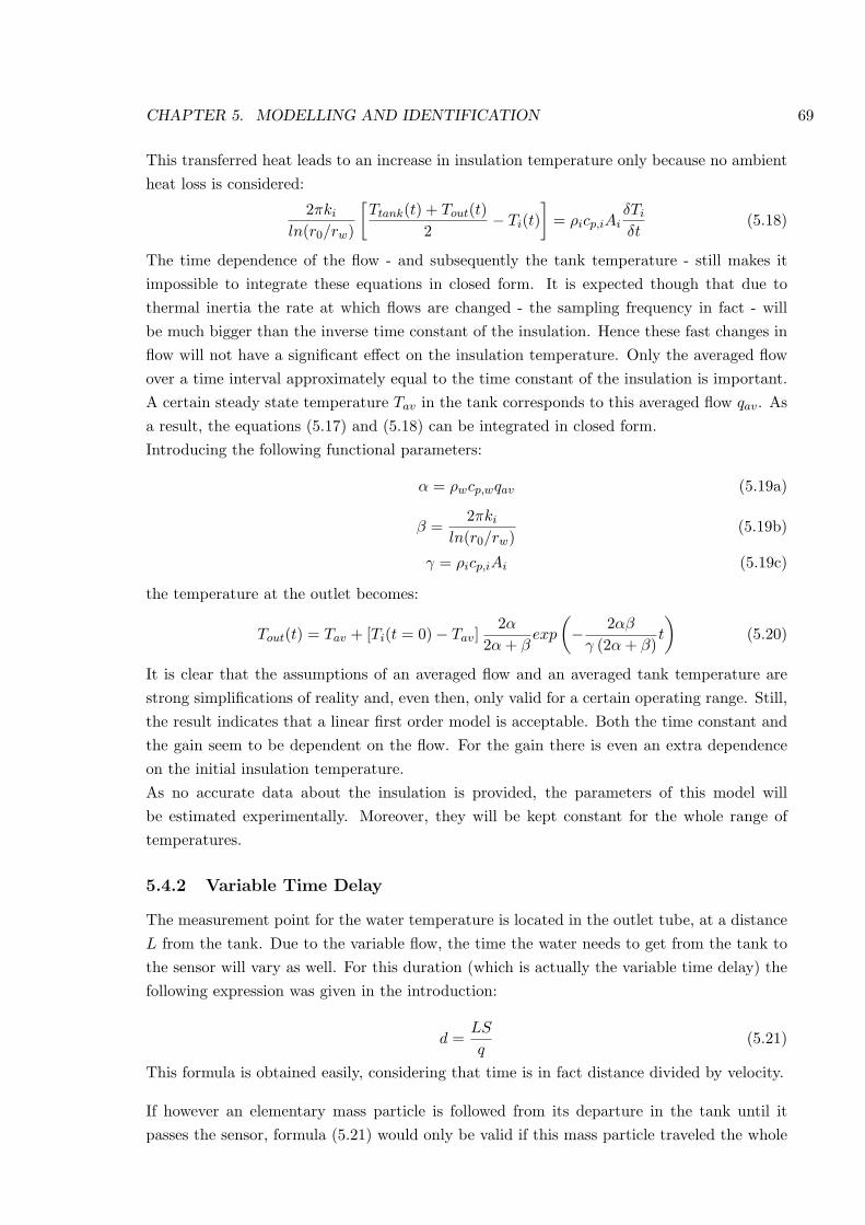
CHAPTER 5. MODELLING AND IDENTIFICATION 69
This transferred heat leads to an increase in insulation temperature only because no ambientheat loss is considered:
2πki
ln(r0/rw)
[Ttank(t) + Tout(t)
2− Ti(t)
]= ρicp,iAi
δTi
δt(5.18)
The time dependence of the flow - and subsequently the tank temperature - still makes itimpossible to integrate these equations in closed form. It is expected though that due tothermal inertia the rate at which flows are changed - the sampling frequency in fact - willbe much bigger than the inverse time constant of the insulation. Hence these fast changes inflow will not have a significant effect on the insulation temperature. Only the averaged flowover a time interval approximately equal to the time constant of the insulation is important.A certain steady state temperature Tav in the tank corresponds to this averaged flow qav. Asa result, the equations (5.17) and (5.18) can be integrated in closed form.Introducing the following functional parameters:
α = ρwcp,wqav (5.19a)
β =2πki
ln(r0/rw)(5.19b)
γ = ρicp,iAi (5.19c)
the temperature at the outlet becomes:
Tout(t) = Tav + [Ti(t = 0)− Tav]2α
2α + βexp
(− 2αβ
γ (2α + β)t
)(5.20)
It is clear that the assumptions of an averaged flow and an averaged tank temperature arestrong simplifications of reality and, even then, only valid for a certain operating range. Still,the result indicates that a linear first order model is acceptable. Both the time constant andthe gain seem to be dependent on the flow. For the gain there is even an extra dependenceon the initial insulation temperature.As no accurate data about the insulation is provided, the parameters of this model willbe estimated experimentally. Moreover, they will be kept constant for the whole range oftemperatures.
5.4.2 Variable Time Delay
The measurement point for the water temperature is located in the outlet tube, at a distanceL from the tank. Due to the variable flow, the time the water needs to get from the tank tothe sensor will vary as well. For this duration (which is actually the variable time delay) thefollowing expression was given in the introduction:
d =LS
q(5.21)
This formula is obtained easily, considering that time is in fact distance divided by velocity.
If however an elementary mass particle is followed from its departure in the tank until itpasses the sensor, formula (5.21) would only be valid if this mass particle traveled the whole
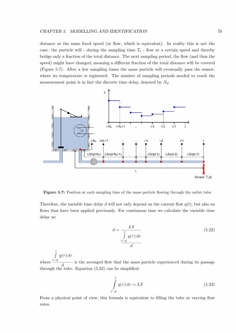
CHAPTER 5. MODELLING AND IDENTIFICATION 70
distance at the same fixed speed (or flow, which is equivalent). In reality this is not thecase: the particle will - during the sampling time Ts - flow at a certain speed and therebybridge only a fraction of the total distance. The next sampling period, the flow (and thus thespeed) might have changed, meaning a different fraction of the total distance will be covered(Figure 5.7). After a few sampling times the mass particle will eventually pass the sensor,where its temperature is registered. The number of sampling periods needed to reach themeasurement point is in fact the discrete time delay, denoted by Nd.
Figure 5.7: Position at each sampling time of the mass particle flowing through the outlet tube
Therefore, the variable time delay d will not only depend on the current flow q(t), but also onflows that have been applied previously. For continuous time we calculate the variable timedelay as:
d =LS
t∫t−d
q(τ) dτ
d
(5.22)
where
t∫t−d
q(τ) dτ
dis the averaged flow that the mass particle experienced during its passage
through the tube. Equation (5.22) can be simplified:
t∫t−d
q(τ) dτ = LS (5.23)
From a physical point of view, this formula is equivalent to filling the tube at varying flowrates.
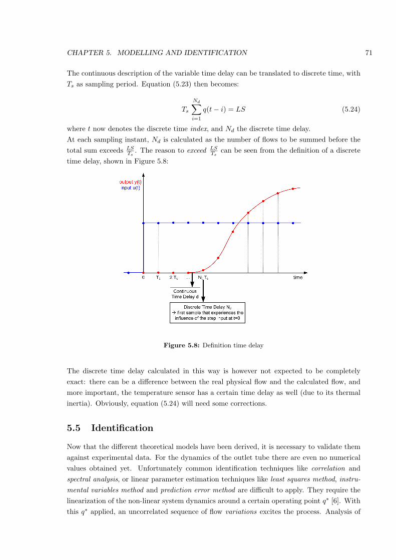
CHAPTER 5. MODELLING AND IDENTIFICATION 71
The continuous description of the variable time delay can be translated to discrete time, withTs as sampling period. Equation (5.23) then becomes:
Ts
Nd∑i=1
q(t− i) = LS (5.24)
where t now denotes the discrete time index, and Nd the discrete time delay.At each sampling instant, Nd is calculated as the number of flows to be summed before thetotal sum exceeds LS
Ts. The reason to exceed LS
Tscan be seen from the definition of a discrete
time delay, shown in Figure 5.8:
Figure 5.8: Definition time delay
The discrete time delay calculated in this way is however not expected to be completelyexact: there can be a difference between the real physical flow and the calculated flow, andmore important, the temperature sensor has a certain time delay as well (due to its thermalinertia). Obviously, equation (5.24) will need some corrections.
5.5 Identification
Now that the different theoretical models have been derived, it is necessary to validate themagainst experimental data. For the dynamics of the outlet tube there are even no numericalvalues obtained yet. Unfortunately common identification techniques like correlation andspectral analysis, or linear parameter estimation techniques like least squares method, instru-mental variables method and prediction error method are difficult to apply. They require thelinearization of the non-linear system dynamics around a certain operating point q∗ [6]. Withthis q∗ applied, an uncorrelated sequence of flow variations excites the process. Analysis of
CHAPTER 5. MODELLING AND IDENTIFICATION 72
the measured temperatures according to one of the previous estimation techniques, leads tothe estimation of parameters which are only valid for the linearization region. As a result,different parameter sets for different linearization regions are obtained. For slowly reactingsystems however - which is the case for thermodynamic processes - it is unlikely that thesesmall and relatively fast changes in input will result in useful temperature changes. Forthe outlet tube these methods would even be more difficult to apply as the input (the tanktemperature in this case) can only be indirectly manipulated.
It seems that the easiest way to perform the validation is to use graphical methods like stepresponses. Moreover, in relatively simple processes like this one, it is expected that thesegraphical methods will be sufficient to have an idea of the accuracy of the theoretical models.First the dynamics of the tank will be discussed, followed by the dynamics of the outlet tube,and - last but not least - the variable time delay.
5.5.1 Water Tank
Here the third measurement of the tank temperature (besides the tap water temperature andtube outlet temperature) finds its relevance. Simple step responses were performed, changingthe flow from a steady state value q1 to a new constant flow q2. The tank dynamics (5.3) arelinearized around q∗ = q2 and written as a transfer function:
Vd∆T (t)
dt= (Tin(t)− T ∗)∆q(t)− q∗∆T (t) (5.25)
(V s + q∗)∆T (s) = (Tin − T ∗)∆q(s) (5.26)
∆T (s)∆q(s)
=Tin − T ∗
V s + q∗(5.27)
∆T (s)∆q(s)
=(Tin − T ∗)/q∗
Vq∗ s + 1
(5.28)
where the steady state temperature T ∗ corresponds to the applied flow q∗, and ∆T and ∆q
are variations around the steady state values T ∗ and q∗. The static gain is given by
Tin − T ∗
q∗(5.29)
whileV
q∗(5.30)
defines the time constant. With ∆q just a step, the solution for this system is an exponentialof the form
Ttank(t) = Tinit + (Tfinal − Tinit)(1− e−t/τ
)(5.31)
with τ the time constant corresponding to q∗. The purpose now is to link the measurementsof the tank temperature to such a first order curve, by graphical identification. Thus, anexperimental time constant and gain are derived, as is shown in Figure 5.9.
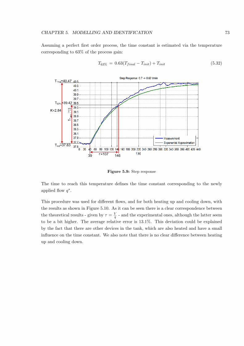
CHAPTER 5. MODELLING AND IDENTIFICATION 73
Assuming a perfect first order process, the time constant is estimated via the temperaturecorresponding to 63% of the process gain:
T63% = 0.63(Tfinal − Tinit) + Tinit (5.32)
Figure 5.9: Step response
The time to reach this temperature defines the time constant corresponding to the newlyapplied flow q∗.
This procedure was used for different flows, and for both heating up and cooling down, withthe results as shown in Figure 5.10. As it can be seen there is a clear correspondence betweenthe theoretical results - given by τ = V
q - and the experimental ones, although the latter seemto be a bit higher. The average relative error is 13.1%. This deviation could be explainedby the fact that there are other devices in the tank, which are also heated and have a smallinfluence on the time constant. We also note that there is no clear difference between heatingup and cooling down.
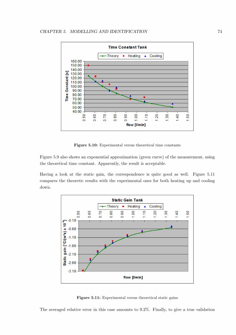
CHAPTER 5. MODELLING AND IDENTIFICATION 74
Figure 5.10: Experimental versus theoretical time constants
Figure 5.9 also shows an exponential approximation (green curve) of the measurement, usingthe theoretical time constant. Apparently, the result is acceptable.
Having a look at the static gain, the correspondence is quite good as well. Figure 5.11compares the theoretic results with the experimental ones for both heating up and coolingdown.
Figure 5.11: Experimental versus theoretical static gains
The averaged relative error in this case amounts to 9.2%. Finally, to give a true validation
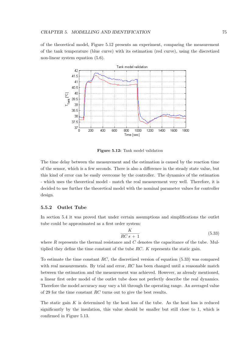
CHAPTER 5. MODELLING AND IDENTIFICATION 75
of the theoretical model, Figure 5.12 presents an experiment, comparing the measurementof the tank temperature (blue curve) with its estimation (red curve), using the discretizednon-linear system equation (5.6).
Figure 5.12: Tank model validation
The time delay between the measurement and the estimation is caused by the reaction timeof the sensor, which is a few seconds. There is also a difference in the steady state value, butthis kind of error can be easily overcome by the controller. The dynamics of the estimation- which uses the theoretical model - match the real measurement very well. Therefore, it isdecided to use further the theoretical model with the nominal parameter values for controllerdesign.
5.5.2 Outlet Tube
In section 5.4 it was proved that under certain assumptions and simplifications the outlettube could be approximated as a first order system:
K
RC s + 1(5.33)
where R represents the thermal resistance and C denotes the capacitance of the tube. Mul-tiplied they define the time constant of the tube RC. K represents the static gain.
To estimate the time constant RC, the discretized version of equation (5.33) was comparedwith real measurements. By trial and error, RC has been changed until a reasonable matchbetween the estimation and the measurement was achieved. However, as already mentioned,a linear first order model of the outlet tube does not perfectly describe the real dynamics.Therefore the model accuracy may vary a bit through the operating range. An averaged valueof 29 for the time constant RC turns out to give the best results.
The static gain K is determined by the heat loss of the tube. As the heat loss is reducedsignificantly by the insulation, this value should be smaller but still close to 1, which isconfirmed in Figure 5.13.
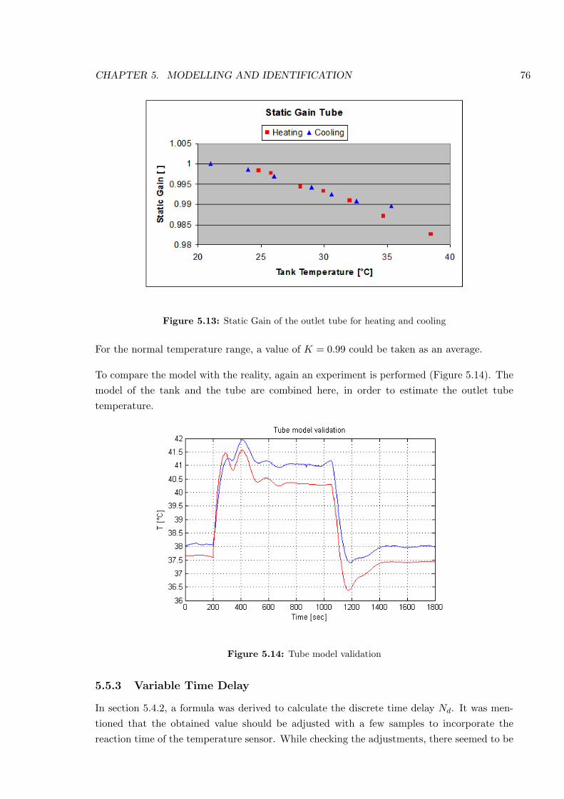
CHAPTER 5. MODELLING AND IDENTIFICATION 76
Figure 5.13: Static Gain of the outlet tube for heating and cooling
For the normal temperature range, a value of K = 0.99 could be taken as an average.
To compare the model with the reality, again an experiment is performed (Figure 5.14). Themodel of the tank and the tube are combined here, in order to estimate the outlet tubetemperature.
Figure 5.14: Tube model validation
5.5.3 Variable Time Delay
In section 5.4.2, a formula was derived to calculate the discrete time delay Nd. It was men-tioned that the obtained value should be adjusted with a few samples to incorporate thereaction time of the temperature sensor. While checking the adjustments, there seemed to be
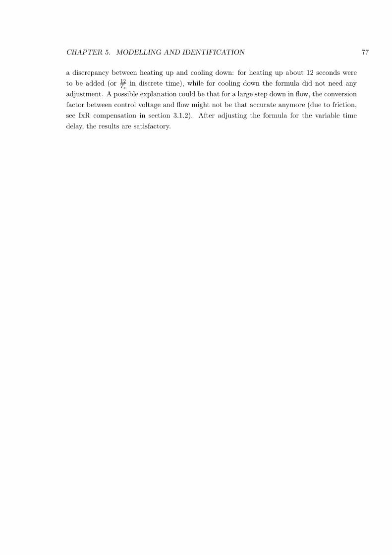
CHAPTER 5. MODELLING AND IDENTIFICATION 77
a discrepancy between heating up and cooling down: for heating up about 12 seconds wereto be added (or 12
Tsin discrete time), while for cooling down the formula did not need any
adjustment. A possible explanation could be that for a large step down in flow, the conversionfactor between control voltage and flow might not be that accurate anymore (due to friction,see IxR compensation in section 3.1.2). After adjusting the formula for the variable timedelay, the results are satisfactory.
Chapter 6
Controllers
The setup as it was designed and implemented in the previous chapters, could in fact bea scale model of a larger industrial application, which shares the problems of non-linearityand huge variable time delay. Such processes are very difficult to control with today’s mostcommon industrial controllers (PID’s). However, with all knowledge packed in process mod-els describing its dynamics, advanced control methods can be implemented. One of theseadvanced control methods uses on-line predictions of the future plant output to compute op-timal future control actions. This control methodology is known as Model Based PredictiveControl (MBPC, also called MPC).In fact, MBPC is a family of control methods that rely on intuitive and easy to understandprinciples. The various MBPC-algorithms differ in the type of model used for prediction andthe criterion they minimize [3]. One of the algorithms that have been used with success inpractice is EPSAC1 [7]. Its inherent dead time compensation and ability to handle non-linearprocess dynamics makes it particularly suited to control the heating tank system. Simulationresults for a similar system, which show the effectiveness of this control strategy can be foundin [5].
This chapter deals with the implementation of the EPSAC-strategy for our setup. Besidesthe difference in scale compared to the system presented in [5], our control problem is morecomplex:
• The tube introduces dynamics into the system.
• Real-life implementation always brings up difficulties that can not be experienced in asimulation environment.
The most important performance-oriented tuning parameters are presented and discussed2.1Non-Linear Extended Prediction Self-Adaptive Control2It is however not the purpose to go into a detailed description of the EPSAC-methodology. For a detailed
description of EPSAC, we refer to [7]. In this case, the controller will be gradually tuned to the process needs
through an analysis of the measured data.
78
CHAPTER 6. CONTROLLERS 79
6.1 Non-linear EPSAC controller
6.1.1 General approach
As in all MBPC-methods, non-linear EPSAC calculates the optimal control input based onpredictions of the output over a certain horizon, called the prediction horizon N2. This is awell known procedure which does not need any adaptation in order to control the heatingtank system with its variable time delay. Before the control loop layout and the influence oftuning parameters are presented, this procedure will be briefly discussed, though specificallyin the interest of the heating tank system.
The future process output, as it is seen by EPSAC, comes from two contributions:
y(t + k|t) = ybase(t + k|t) + yopt(t + k|t) k = 1..N2 (6.1)
1. [ybase(t + k|t), k = 1..N2] is the basic output which originates from several effects:
• past control inputs [u(t− 1), u(t− 2), u(t− 3), ...]. These inputs have been appliedto the process and hence, their effect on the output can be predicted based on theprocess model and its state [x(t− 1), x(t− 2), x(t− 3), ...]. Obviously, for a systemwith a large time delay, many past inputs will have to be taken into account.
• the basic future control scenario [ubase(t + k|t), k = 0..N2 − 1], which is a postu-lated input sequence. This is part of the optimal control scenario to be calculatedby EPSAC. The choice of ubase is irrelevant for linear systems: any choice will leadto the same optimized control input sequence. For non-linear systems though, agood ‘guess’ of ubase has to be made in order to reduce computation time.
• predicted disturbances [n(t + k|t), k = 1..N2]. These predictions are calculated viaa noise model which captures - ideally - all effects in the measured output y(t)that are not included in the process model itself. Out of these effects, the mostobvious are the modelling errors, measurement noise and random disturbances.A smart choice of the noise model can enhance the controller’s performance sig-nificantly since more information about the process is provided to the controller.However, deriving a good noise model is hard, precisely due to the random natureof the disturbances. Most of the time, a default noise model of the form 1
1−q−1 isimplemented. As this default model can only deal with steady state errors, effortwill be taken to derive a more accurate model. This must be seen as a part ofthe controller tuning as the improved noise model is only relevant for the processunder consideration.
2. [yopt(t + k|t), k = 1..N2] is the result of the future optimizing control actions[δu(t + k|t), k = 0..N2 − 1]. These optimizing control actions are the second part ofthe optimal control scenario, which is obtained by adding them to the a priori definedbasic input:
u(t + k|t) = ubase(t + k|t) + δuopt(t + k|t) k = 0..N2 − 1 (6.2)
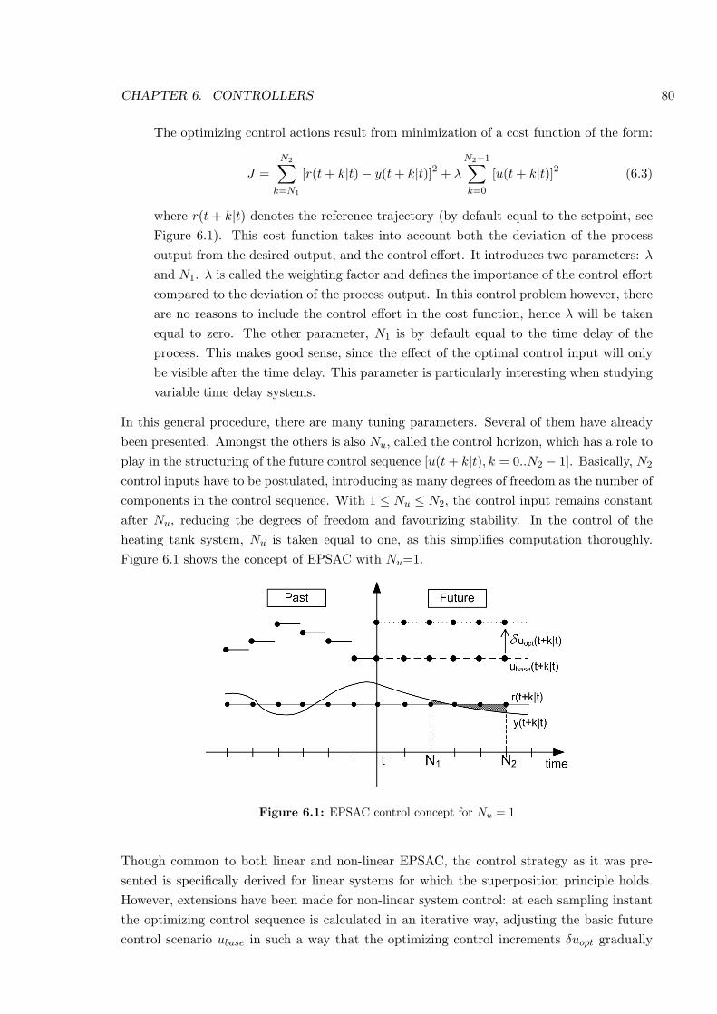
CHAPTER 6. CONTROLLERS 80
The optimizing control actions result from minimization of a cost function of the form:
J =N2∑
k=N1
[r(t + k|t)− y(t + k|t)]2 + λ
N2−1∑k=0
[u(t + k|t)]2 (6.3)
where r(t + k|t) denotes the reference trajectory (by default equal to the setpoint, seeFigure 6.1). This cost function takes into account both the deviation of the processoutput from the desired output, and the control effort. It introduces two parameters: λ
and N1. λ is called the weighting factor and defines the importance of the control effortcompared to the deviation of the process output. In this control problem however, thereare no reasons to include the control effort in the cost function, hence λ will be takenequal to zero. The other parameter, N1 is by default equal to the time delay of theprocess. This makes good sense, since the effect of the optimal control input will onlybe visible after the time delay. This parameter is particularly interesting when studyingvariable time delay systems.
In this general procedure, there are many tuning parameters. Several of them have alreadybeen presented. Amongst the others is also Nu, called the control horizon, which has a role toplay in the structuring of the future control sequence [u(t + k|t), k = 0..N2 − 1]. Basically, N2
control inputs have to be postulated, introducing as many degrees of freedom as the number ofcomponents in the control sequence. With 1 ≤ Nu ≤ N2, the control input remains constantafter Nu, reducing the degrees of freedom and favourizing stability. In the control of theheating tank system, Nu is taken equal to one, as this simplifies computation thoroughly.Figure 6.1 shows the concept of EPSAC with Nu=1.
Figure 6.1: EPSAC control concept for Nu = 1
Though common to both linear and non-linear EPSAC, the control strategy as it was pre-sented is specifically derived for linear systems for which the superposition principle holds.However, extensions have been made for non-linear system control: at each sampling instantthe optimizing control sequence is calculated in an iterative way, adjusting the basic futurecontrol scenario ubase in such a way that the optimizing control increments δuopt gradually
CHAPTER 6. CONTROLLERS 81
go to zero. In this way, the superposition principle is no longer involved and the basic con-trol scenario ubase converges to the optimal solution. To limit the number of iterations andhence the computation time, it is important to make a good initial ‘guess’ for the basic futurecontrol scenario. An effective choice for ubase is the previously applied optimal control input:ubase(t+k|t) ≡ u(t−1). This approach will also be implemented in the control of the heatingtank system. The number of iterations will be referred to as Ni.
As already mentioned, the optimal control actions are calculated by minimizing the costfunction (6.3), rewritten in matrix notations, with Y and R the future process output andthe reference trajectory respectively:
J =N2∑
k=N1
[r(t + k|t)− y(t + k|t)]2 = (R−Y)T (R−Y) (6.4)
In the specific case of Nu = 1, the sequence of optimizing control actions is simplified to[δu(t + k|t) ≡ δu(t|t)]. This can be seen as a step input with magnitude δu, applied at timet. Hence, yopt can be calculated as a step response.For non-linear systems the step responses at every iteration can be calculated in two ways:through simulation based on the non-linear process model, or through local linearization.This last calculation procedure is implemented in this case: every iteration, the process islinearized around ubase (which is in turn iteratively adapted) to extract its step coefficientsgk. As a result, yopt is calculated as:
yopt =
gN1
gN1+1
...
gN2
δu = G · δu (6.5)
Substituting this expression into equation (6.4), the cost function appears as a function of δu:
N2∑k=N1
[r(t + k|t)− y(t + k|t)]2 = ((R−Ybase)−G · δu)T ((R−Ybase)−G · δu) (6.6)
The minimum cost index is obtained for
δu =(GTG
)−1GT (R−Y) (6.7)
6.1.2 Control loop layout
For output prediction, two model configurations are possible: one is the parallel model, theother one is the series-parallel model. The first one can only be used for stable processes, whilethe second can also be used for unstable processes. Since the process under consideration isstable, the implementation of the parallel model as depicted in Figure 6.2 is used.
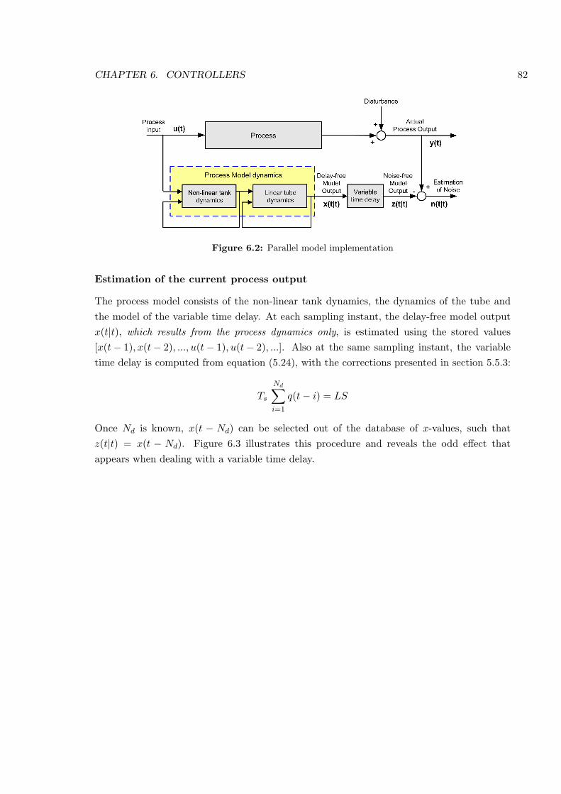
CHAPTER 6. CONTROLLERS 82
Figure 6.2: Parallel model implementation
Estimation of the current process output
The process model consists of the non-linear tank dynamics, the dynamics of the tube andthe model of the variable time delay. At each sampling instant, the delay-free model outputx(t|t), which results from the process dynamics only, is estimated using the stored values[x(t− 1), x(t− 2), ..., u(t− 1), u(t− 2), ...]. Also at the same sampling instant, the variabletime delay is computed from equation (5.24), with the corrections presented in section 5.5.3:
Ts
Nd∑i=1
q(t− i) = LS
Once Nd is known, x(t − Nd) can be selected out of the database of x-values, such thatz(t|t) = x(t − Nd). Figure 6.3 illustrates this procedure and reveals the odd effect thatappears when dealing with a variable time delay.
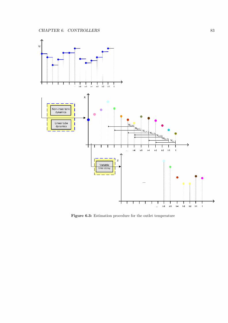
CHAPTER 6. CONTROLLERS 83
Figure 6.3: Estimation procedure for the outlet temperature
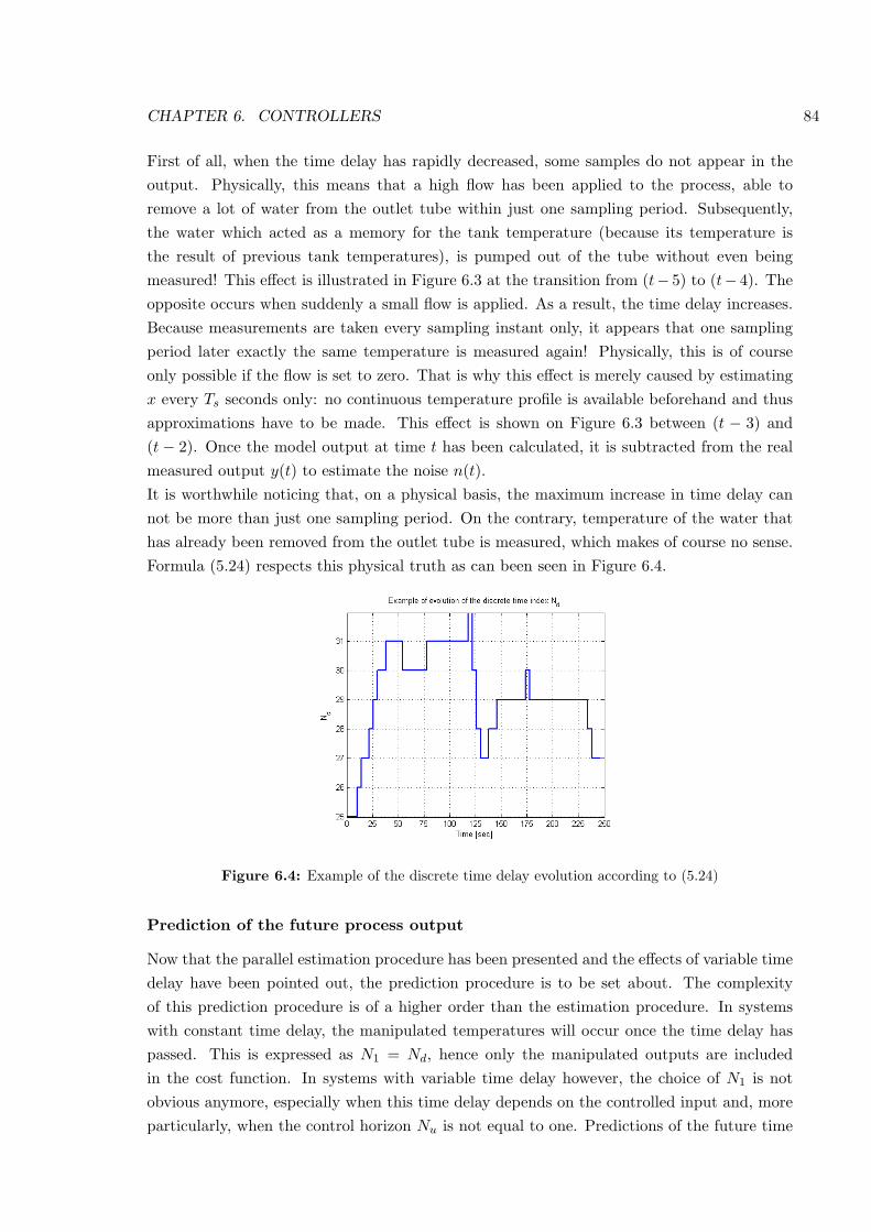
CHAPTER 6. CONTROLLERS 84
First of all, when the time delay has rapidly decreased, some samples do not appear in theoutput. Physically, this means that a high flow has been applied to the process, able toremove a lot of water from the outlet tube within just one sampling period. Subsequently,the water which acted as a memory for the tank temperature (because its temperature isthe result of previous tank temperatures), is pumped out of the tube without even beingmeasured! This effect is illustrated in Figure 6.3 at the transition from (t− 5) to (t− 4). Theopposite occurs when suddenly a small flow is applied. As a result, the time delay increases.Because measurements are taken every sampling instant only, it appears that one samplingperiod later exactly the same temperature is measured again! Physically, this is of courseonly possible if the flow is set to zero. That is why this effect is merely caused by estimatingx every Ts seconds only: no continuous temperature profile is available beforehand and thusapproximations have to be made. This effect is shown on Figure 6.3 between (t − 3) and(t− 2). Once the model output at time t has been calculated, it is subtracted from the realmeasured output y(t) to estimate the noise n(t).It is worthwhile noticing that, on a physical basis, the maximum increase in time delay cannot be more than just one sampling period. On the contrary, temperature of the water thathas already been removed from the outlet tube is measured, which makes of course no sense.Formula (5.24) respects this physical truth as can been seen in Figure 6.4.
Figure 6.4: Example of the discrete time delay evolution according to (5.24)
Prediction of the future process output
Now that the parallel estimation procedure has been presented and the effects of variable timedelay have been pointed out, the prediction procedure is to be set about. The complexityof this prediction procedure is of a higher order than the estimation procedure. In systemswith constant time delay, the manipulated temperatures will occur once the time delay haspassed. This is expressed as N1 = Nd, hence only the manipulated outputs are includedin the cost function. In systems with variable time delay however, the choice of N1 is notobvious anymore, especially when this time delay depends on the controlled input and, moreparticularly, when the control horizon Nu is not equal to one. Predictions of the future time
CHAPTER 6. CONTROLLERS 85
delay should be made in order to determine the temperature profile at the output to be ableto extract only that part which results from the future flows. Hence, it is not straightforwardwhat the value of N1 should be.In many practical applications however, the simplification of Nu = 1 has lead to amazinglygood results [7]. Therefore it is not expected that this assumption will significantly affect thecontroller’s performance. Additionally, in this case it would reduce complexity greatly. Thatis why only Nu = 1 will be considered3.
Basically, the prediction procedure goes in the same way as the estimation procedure. At eachsampling instant, predictions [x(t+k|t), k = 1..N2] are made, using the postulated future con-trol sequence qbase as input and the previously estimated values [x(t), x(t− 1), ...] as the cur-rent state of the system. Then, the variable time delay is computed to select the appropriatex((t + k) −Nd) as the prediction of the outlet temperature z(t + k|t). Only the predictions[z(t + k|t), k = N1..N2] are included in the cost function because they are manipulated byqbase. This procedure is illustrated in Figure 6.5.
This strategy is very time consuming due to the number of calculations involved. First of all,the states x(t+k|t) must be predicted; secondly, for each single state prediction the algorithmto calculate the variable time delay has to be called in order to obtain the future time delays;and thirdly, appropriate selections must be made to compose the future temperature profileat the output. Only a part of this profile is used, namely from N1 (which varies as well)to N2. Enough predictions must be included in the cost function to have a stable closedloop and reasonable performance (see section 6.1.4). Consequently, the prediction horizonN2 must be chosen with respect to N1, which makes it variable as well4. This in turn meansthat the number of predictions x(t + k|t) is not just a straightforward value. That is why theprediction procedure is far more complex than might be assumed initially. It requires a lot ofcalculations and is difficult to implement.
3Taking Nu = 1 means no degrees of freedom are left to optimize the control input with respect to its
constraints. Hence, the method of clipping is implemented after the EPSAC computation of the optimal
input.4For example, N2 = N1 + C where C denotes the number of samples in the cost function.
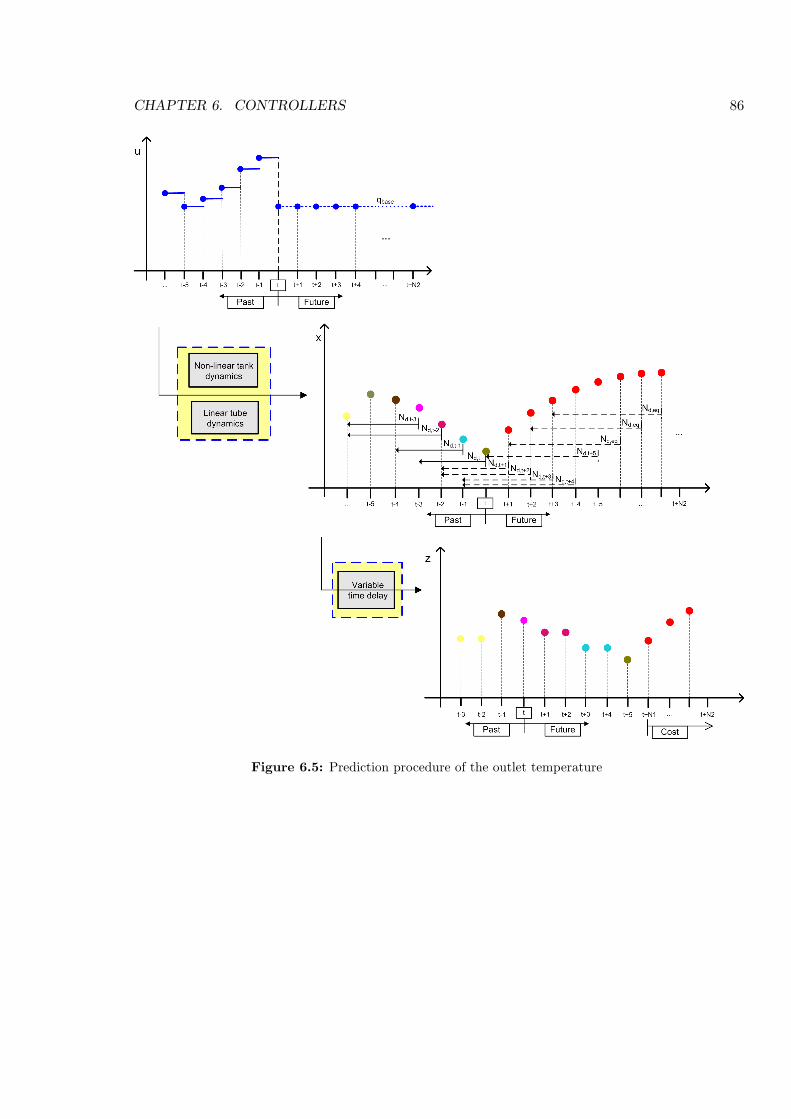
CHAPTER 6. CONTROLLERS 86
Figure 6.5: Prediction procedure of the outlet temperature
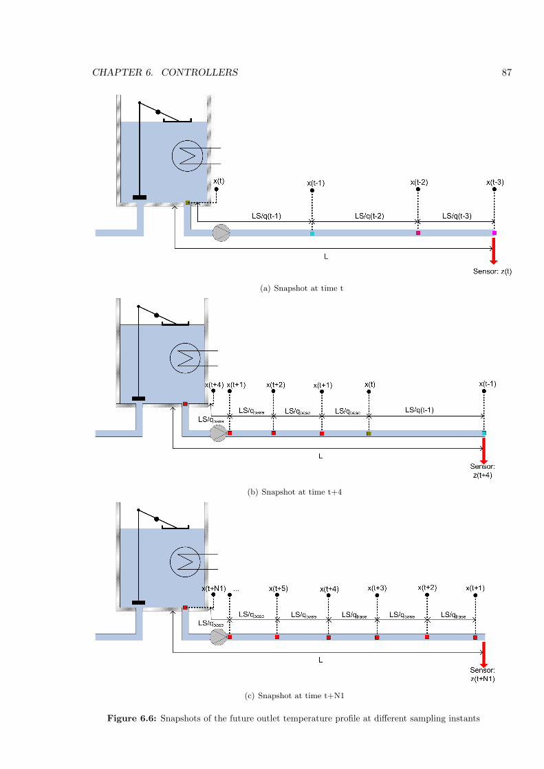
CHAPTER 6. CONTROLLERS 87
(a) Snapshot at time t
(b) Snapshot at time t+4
(c) Snapshot at time t+N1
Figure 6.6: Snapshots of the future outlet temperature profile at different sampling instants
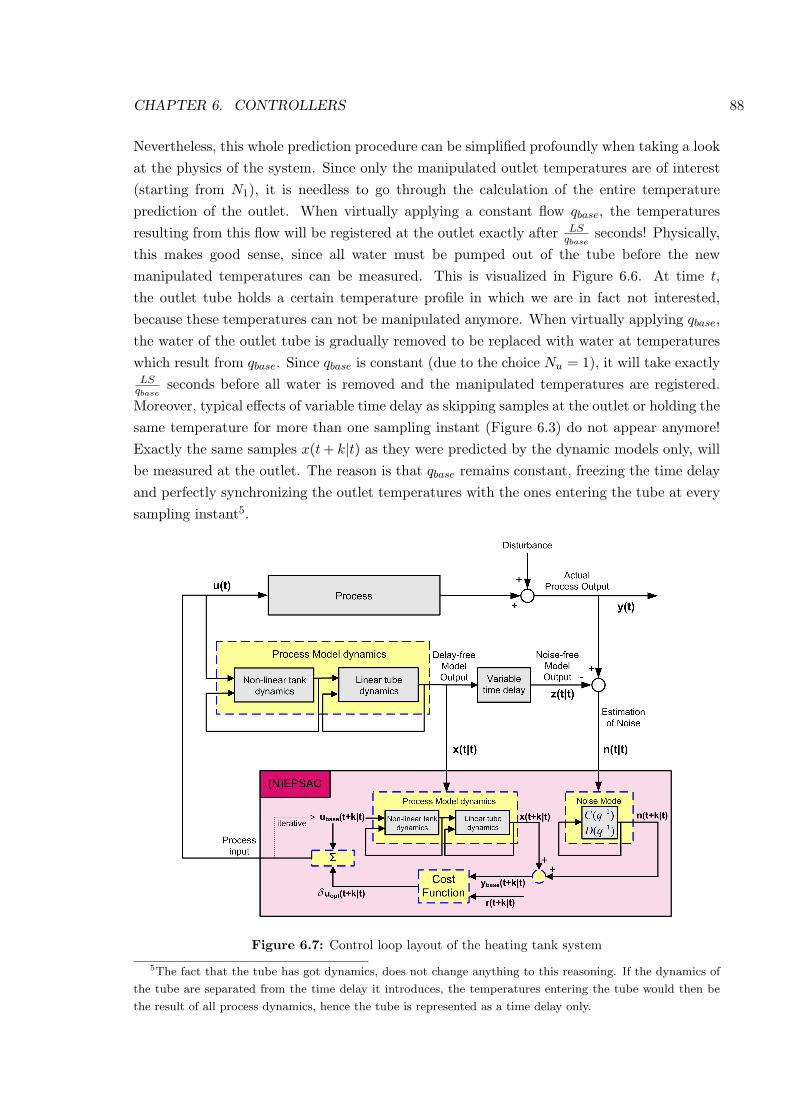
CHAPTER 6. CONTROLLERS 88
Nevertheless, this whole prediction procedure can be simplified profoundly when taking a lookat the physics of the system. Since only the manipulated outlet temperatures are of interest(starting from N1), it is needless to go through the calculation of the entire temperatureprediction of the outlet. When virtually applying a constant flow qbase, the temperaturesresulting from this flow will be registered at the outlet exactly after LS
qbaseseconds! Physically,
this makes good sense, since all water must be pumped out of the tube before the newmanipulated temperatures can be measured. This is visualized in Figure 6.6. At time t,the outlet tube holds a certain temperature profile in which we are in fact not interested,because these temperatures can not be manipulated anymore. When virtually applying qbase,the water of the outlet tube is gradually removed to be replaced with water at temperatureswhich result from qbase. Since qbase is constant (due to the choice Nu = 1), it will take exactlyLS
qbaseseconds before all water is removed and the manipulated temperatures are registered.
Moreover, typical effects of variable time delay as skipping samples at the outlet or holding thesame temperature for more than one sampling instant (Figure 6.3) do not appear anymore!Exactly the same samples x(t + k|t) as they were predicted by the dynamic models only, willbe measured at the outlet. The reason is that qbase remains constant, freezing the time delayand perfectly synchronizing the outlet temperatures with the ones entering the tube at everysampling instant5.
Figure 6.7: Control loop layout of the heating tank system
5The fact that the tube has got dynamics, does not change anything to this reasoning. If the dynamics of
the tube are separated from the time delay it introduces, the temperatures entering the tube would then be
the result of all process dynamics, hence the tube is represented as a time delay only.
CHAPTER 6. CONTROLLERS 89
Consequently, it is sufficient just to predict the temperatures resulting from the dynamics,without predicting the entire outlet temperature profile. It is important to stress however thateven though this profile is not calculated as such, the outlet temperature is still the controlledvariable! Going through the explicit procedure (as presented in Figure 6.3) would exactlylead to the same result, but would require much more effort and much more complexity tobe overcome. In this way, the prediction procedure is thoroughly simplified. N1 is no longervarying and obviously equal to one. Hence, N2 is also constant. The variable time delay modelis only used for noise computation. The non-linear EPSAC-structure as it is implemented forthe heating tank system is presented in Figure 6.7.
6.1.3 Choice of Ts
Before any computer control can be implemented, the sampling time Ts must be chosen. Sincethe measured signals are fed through lowpass filters having a cutoff frequency of 1.1 Hz, alias-ing will not occur if the sampling frequency is at least double, which is the Nyquist frequencyin this case. However, the bandwidth of the system - linearized around the maximum flow -is approximately 0.004 Hz, which is far less than the proposed sampling frequency. In ordernot to overload the computer needlessly, a choice has to be made without the risk of mixingup high frequency disturbances with the signals of interest. That is why the sampling rate ischosen equal to 5 Hz, so that no aliasing can occur. The higher frequency signals are filteredout through averaging over a certain period. This period is the sampling time Ts used tocontrol the system.
To determine Ts, there is a commonly accepted rule of thumb proposing the sampling timeto be approximately one tenth of the system time constant. In this case, the time constantis varying. A conservative choice for Ts would be the one resulting from the smallest timeconstant:
τmin =V
qmax=
1.13 l
1.8 l/min= 37.7 sec (6.8)
This means that Ts should be around 4 seconds. Still, there is an experimental part in thechoice of Ts as well. If Ts is chosen too large, it would limit the freedom of the controller torapidly adjust the input in order to get the temperature to the setpoint as fast as possible.Secondly, a large Ts leads to poor discretization of the non-linear model and consequently topoor estimations. On the other hand, taking Ts too small would probably make the controllertoo sensitive and increase the computer workload needlessly. After several experiments withdifferent sampling times, it turned out that the best choice would be to take Ts equal to4 seconds.
6.1.4 Influence of N2
The prediction horizon N2 determines the number of predictions made starting from timet + 1. Based on these predictions, the optimal control strategy is calculated to minimize thecost function. Even though there is no general rule for selecting N2 appropriately, its choiceis indeed of crucial importance for the controller’s performance.
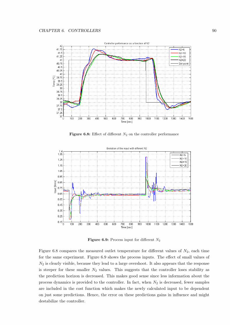
CHAPTER 6. CONTROLLERS 90
Figure 6.8: Effect of different N2 on the controller performance
Figure 6.9: Process input for different N2
Figure 6.8 compares the measured outlet temperature for different values of N2, each timefor the same experiment. Figure 6.9 shows the process inputs. The effect of small values ofN2 is clearly visible, because they lead to a large overshoot. It also appears that the responseis steeper for these smaller N2 values. This suggests that the controller loses stability asthe prediction horizon is decreased. This makes good sense since less information about theprocess dynamics is provided to the controller. In fact, when N2 is decreased, fewer samplesare included in the cost function which makes the newly calculated input to be dependenton just some predictions. Hence, the error on these predictions gains in influence and mightdestabilize the controller.
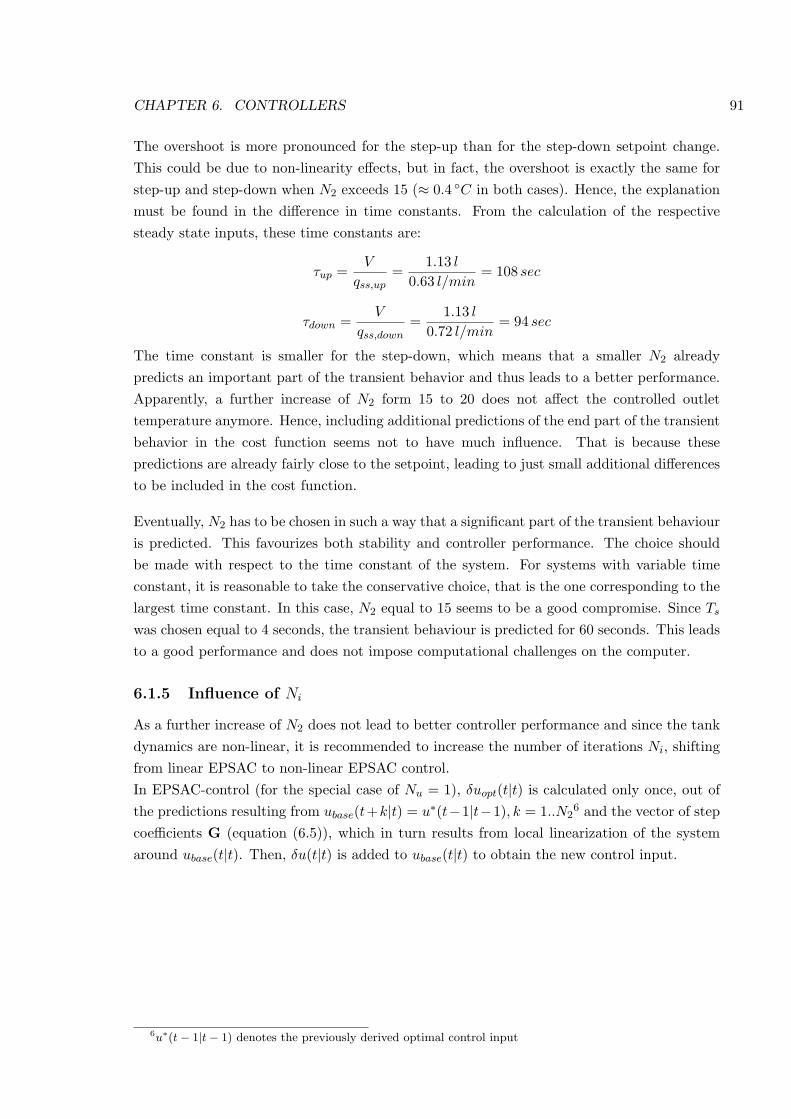
CHAPTER 6. CONTROLLERS 91
The overshoot is more pronounced for the step-up than for the step-down setpoint change.This could be due to non-linearity effects, but in fact, the overshoot is exactly the same forstep-up and step-down when N2 exceeds 15 (≈ 0.4 C in both cases). Hence, the explanationmust be found in the difference in time constants. From the calculation of the respectivesteady state inputs, these time constants are:
τup =V
qss,up=
1.13 l
0.63 l/min= 108 sec
τdown =V
qss,down=
1.13 l
0.72 l/min= 94 sec
The time constant is smaller for the step-down, which means that a smaller N2 alreadypredicts an important part of the transient behavior and thus leads to a better performance.Apparently, a further increase of N2 form 15 to 20 does not affect the controlled outlettemperature anymore. Hence, including additional predictions of the end part of the transientbehavior in the cost function seems not to have much influence. That is because thesepredictions are already fairly close to the setpoint, leading to just small additional differencesto be included in the cost function.
Eventually, N2 has to be chosen in such a way that a significant part of the transient behaviouris predicted. This favourizes both stability and controller performance. The choice shouldbe made with respect to the time constant of the system. For systems with variable timeconstant, it is reasonable to take the conservative choice, that is the one corresponding to thelargest time constant. In this case, N2 equal to 15 seems to be a good compromise. Since Ts
was chosen equal to 4 seconds, the transient behaviour is predicted for 60 seconds. This leadsto a good performance and does not impose computational challenges on the computer.
6.1.5 Influence of Ni
As a further increase of N2 does not lead to better controller performance and since the tankdynamics are non-linear, it is recommended to increase the number of iterations Ni, shiftingfrom linear EPSAC to non-linear EPSAC control.In EPSAC-control (for the special case of Nu = 1), δuopt(t|t) is calculated only once, out ofthe predictions resulting from ubase(t+k|t) = u∗(t−1|t−1), k = 1..N2
6 and the vector of stepcoefficients G (equation (6.5)), which in turn results from local linearization of the systemaround ubase(t|t). Then, δu(t|t) is added to ubase(t|t) to obtain the new control input.
6u∗(t − 1|t − 1) denotes the previously derived optimal control input
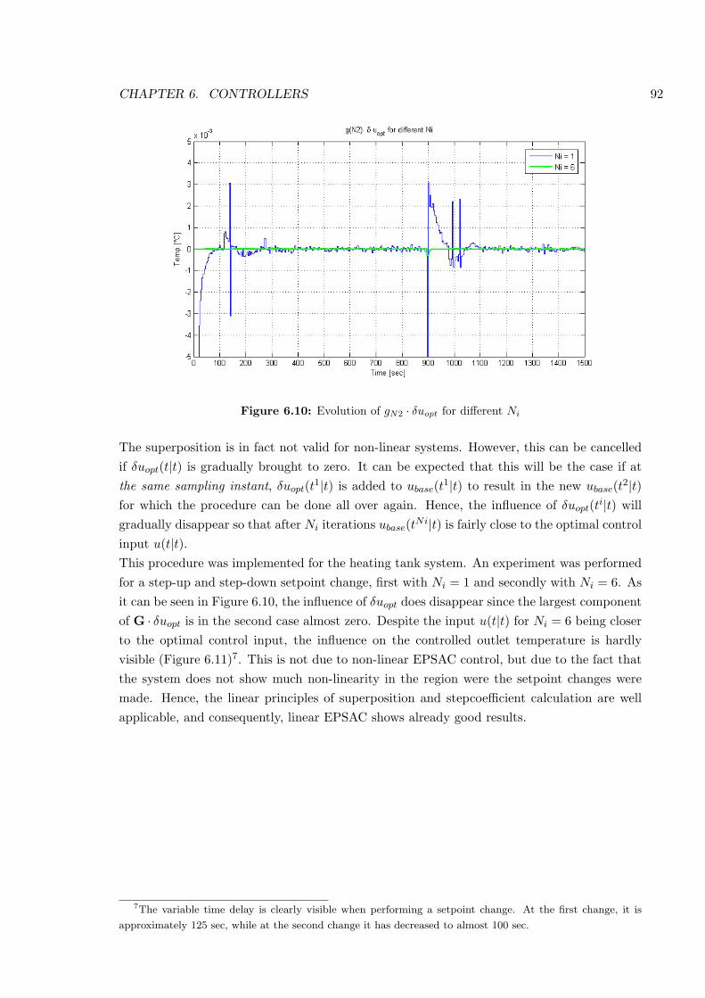
CHAPTER 6. CONTROLLERS 92
Figure 6.10: Evolution of gN2 · δuopt for different Ni
The superposition is in fact not valid for non-linear systems. However, this can be cancelledif δuopt(t|t) is gradually brought to zero. It can be expected that this will be the case if atthe same sampling instant, δuopt(t1|t) is added to ubase(t1|t) to result in the new ubase(t2|t)for which the procedure can be done all over again. Hence, the influence of δuopt(ti|t) willgradually disappear so that after Ni iterations ubase(tNi|t) is fairly close to the optimal controlinput u(t|t).This procedure was implemented for the heating tank system. An experiment was performedfor a step-up and step-down setpoint change, first with Ni = 1 and secondly with Ni = 6. Asit can be seen in Figure 6.10, the influence of δuopt does disappear since the largest componentof G · δuopt is in the second case almost zero. Despite the input u(t|t) for Ni = 6 being closerto the optimal control input, the influence on the controlled outlet temperature is hardlyvisible (Figure 6.11)7. This is not due to non-linear EPSAC control, but due to the fact thatthe system does not show much non-linearity in the region were the setpoint changes weremade. Hence, the linear principles of superposition and stepcoefficient calculation are wellapplicable, and consequently, linear EPSAC shows already good results.
7The variable time delay is clearly visible when performing a setpoint change. At the first change, it is
approximately 125 sec, while at the second change it has decreased to almost 100 sec.
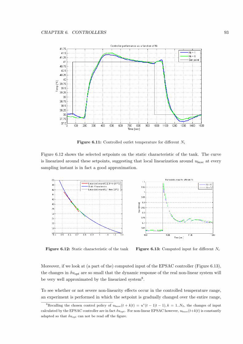
CHAPTER 6. CONTROLLERS 93
Figure 6.11: Controlled outlet temperature for different Ni
Figure 6.12 shows the selected setpoints on the static characteristic of the tank. The curveis linearized around these setpoints, suggesting that local linearization around ubase at everysampling instant is in fact a good approximation.
Figure 6.12: Static characteristic of the tank Figure 6.13: Computed input for different Ni
Moreover, if we look at (a part of the) computed input of the EPSAC controller (Figure 6.13),the changes in δuopt are so small that the dynamic response of the real non-linear system willbe very well approximated by the linearized system8.
To see whether or not severe non-linearity effects occur in the controlled temperature range,an experiment is performed in which the setpoint is gradually changed over the entire range,
8Recalling the chosen control policy of ubase(t + k|t) = u∗(t − 1|t − 1), k = 1..N2, the changes of input
calculated by the EPSAC controller are in fact δuopt. For non-linear EPSAC however, ubase(t+k|t) is constantly
adapted so that δuopt can not be read off the figure.
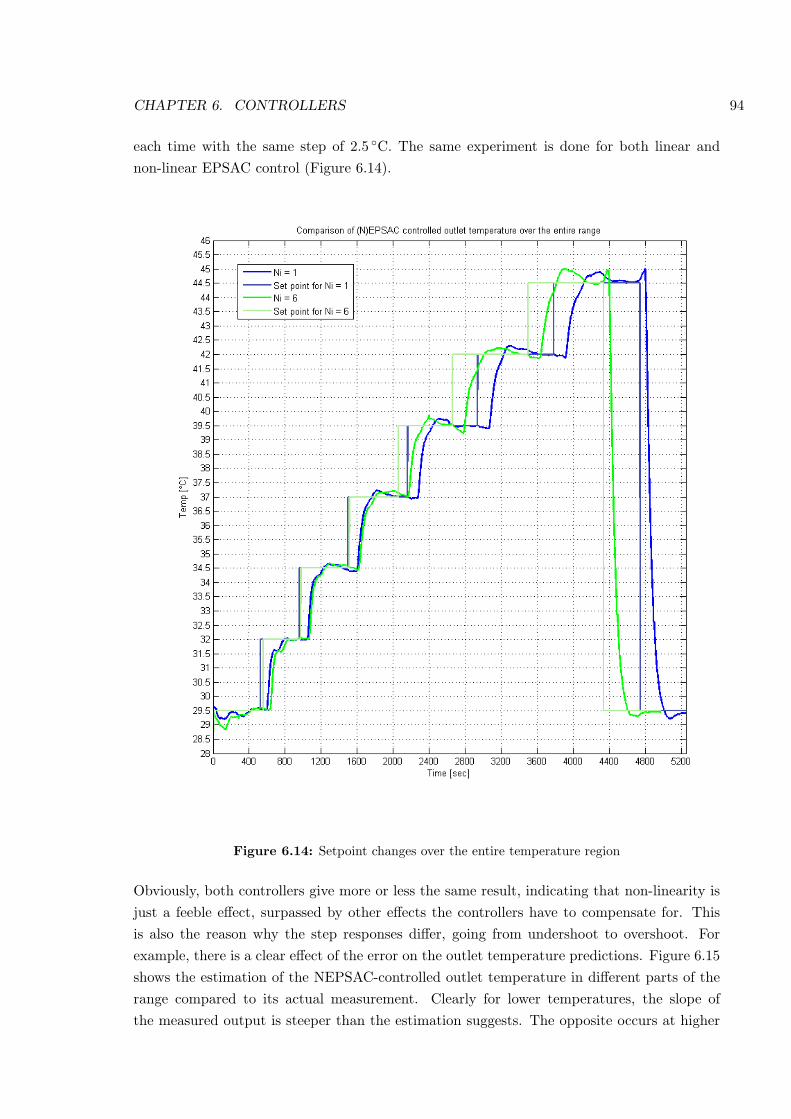
CHAPTER 6. CONTROLLERS 94
each time with the same step of 2.5 C. The same experiment is done for both linear andnon-linear EPSAC control (Figure 6.14).
Figure 6.14: Setpoint changes over the entire temperature region
Obviously, both controllers give more or less the same result, indicating that non-linearity isjust a feeble effect, surpassed by other effects the controllers have to compensate for. Thisis also the reason why the step responses differ, going from undershoot to overshoot. Forexample, there is a clear effect of the error on the outlet temperature predictions. Figure 6.15shows the estimation of the NEPSAC-controlled outlet temperature in different parts of therange compared to its actual measurement. Clearly for lower temperatures, the slope ofthe measured output is steeper than the estimation suggests. The opposite occurs at higher
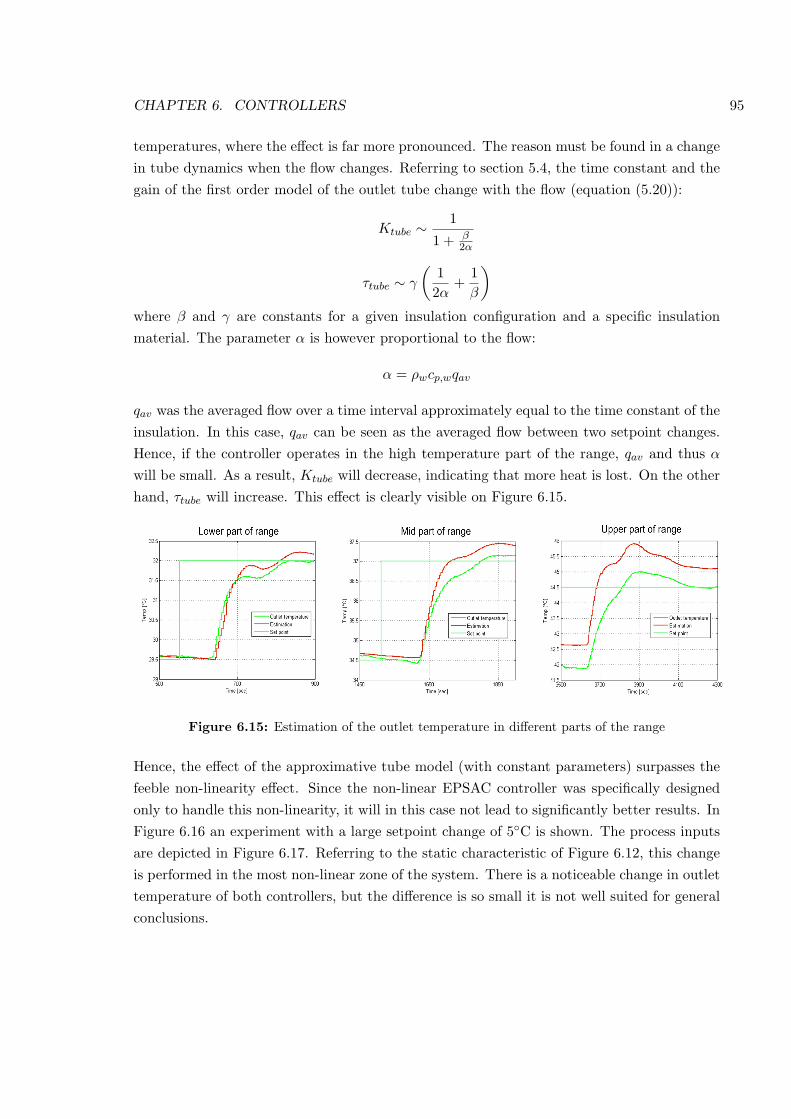
CHAPTER 6. CONTROLLERS 95
temperatures, where the effect is far more pronounced. The reason must be found in a changein tube dynamics when the flow changes. Referring to section 5.4, the time constant and thegain of the first order model of the outlet tube change with the flow (equation (5.20)):
Ktube ∼1
1 + β2α
τtube ∼ γ
(12α
+1β
)where β and γ are constants for a given insulation configuration and a specific insulationmaterial. The parameter α is however proportional to the flow:
α = ρwcp,wqav
qav was the averaged flow over a time interval approximately equal to the time constant of theinsulation. In this case, qav can be seen as the averaged flow between two setpoint changes.Hence, if the controller operates in the high temperature part of the range, qav and thus α
will be small. As a result, Ktube will decrease, indicating that more heat is lost. On the otherhand, τtube will increase. This effect is clearly visible on Figure 6.15.
Figure 6.15: Estimation of the outlet temperature in different parts of the range
Hence, the effect of the approximative tube model (with constant parameters) surpasses thefeeble non-linearity effect. Since the non-linear EPSAC controller was specifically designedonly to handle this non-linearity, it will in this case not lead to significantly better results. InFigure 6.16 an experiment with a large setpoint change of 5C is shown. The process inputsare depicted in Figure 6.17. Referring to the static characteristic of Figure 6.12, this changeis performed in the most non-linear zone of the system. There is a noticeable change in outlettemperature of both controllers, but the difference is so small it is not well suited for generalconclusions.
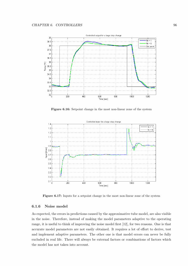
CHAPTER 6. CONTROLLERS 96
Figure 6.16: Setpoint change in the most non-linear zone of the system
Figure 6.17: Inputs for a setpoint change in the most non-linear zone of the system
6.1.6 Noise model
As expected, the errors in predictions caused by the approximative tube model, are also visiblein the noise. Therefore, instead of making the model parameters adaptive to the operatingrange, it is useful to think of improving the noise model first [12], for two reasons. One is thataccurate model parameters are not easily obtained. It requires a lot of effort to derive, testand implement adaptive parameters. The other one is that model errors can never be fullyexcluded in real life. There will always be external factors or combinations of factors whichthe model has not taken into account.
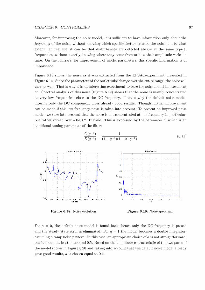
CHAPTER 6. CONTROLLERS 97
Moreover, for improving the noise model, it is sufficient to have information only about thefrequency of the noise, without knowing which specific factors created the noise and to whatextent. In real life, it can be that disturbances are detected always at the same typicalfrequencies, without exactly knowing where they come from or how their amplitude varies intime. On the contrary, for improvement of model parameters, this specific information is ofimportance.
Figure 6.18 shows the noise as it was extracted from the EPSAC-experiment presented inFigure 6.14. Since the parameters of the outlet tube change over the entire range, the noise willvary as well. That is why it is an interesting experiment to base the noise model improvementon. Spectral analysis of this noise (Figure 6.19) shows that the noise is mainly concentratedat very low frequencies, close to the DC-frequency. That is why the default noise model,filtering only the DC component, gives already good results. Though further improvementcan be made if this low frequency noise is taken into account. To present an improved noisemodel, we take into account that the noise is not concentrated at one frequency in particular,but rather spread over a 0-0.02 Hz band. This is expressed by the parameter a, which is anadditional tuning parameter of the filter:
C(q−1)D(q−1)
=1
(1− q−1)(1− a · q−1)(6.11)
Figure 6.18: Noise evolution Figure 6.19: Noise spectrum
For a = 0, the default noise model is found back, hence only the DC-frequency is passedand the steady state error is eliminated. For a = 1 the model becomes a double integrator,assuming a ramp noise pattern. In this case, an appropriate choice of a is not straightforward,but it should at least be around 0.5. Based on the amplitude characteristic of the two parts ofthe model shown in Figure 6.20 and taking into account that the default noise model alreadygave good results, a is chosen equal to 0.4.
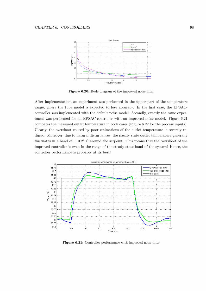
CHAPTER 6. CONTROLLERS 98
Figure 6.20: Bode diagram of the improved noise filter
After implementation, an experiment was performed in the upper part of the temperaturerange, where the tube model is expected to lose accuracy. In the first case, the EPSAC-controller was implemented with the default noise model. Secondly, exactly the same exper-iment was performed for an EPSAC-controller with an improved noise model. Figure 6.21compares the measured outlet temperature in both cases (Figure 6.22 for the process inputs).Clearly, the overshoot caused by poor estimations of the outlet temperature is severely re-duced. Moreover, due to natural disturbances, the steady state outlet temperature generallyfluctuates in a band of ± 0.2 C around the setpoint. This means that the overshoot of theimproved controller is even in the range of the steady state band of the system! Hence, thecontroller performance is probably at its best!
Figure 6.21: Controller performance with improved noise filter
CHAPTER 6. CONTROLLERS 99
Figure 6.22: Process input with default and improved noise filter
6.2 Genuine PI-controller and Smith predictor
To give an idea how well the tuned EPSAC controller performs, both a genuine PI-controllerand a PI-controller in the Smith predictor control-loop layout were implemented. The choicefor a genuine PI-controller might be seen as ‘unfair’ because it does not make use of any pre-dictions and is therefore not aware of neither variable time delay nor non-linearity. Though,in spite of all advances in process control, the PI-controller is still the most commonly en-countered controller in the process industry. PI-controllers can address delays in the systemdynamics, but serious practical limitations are reached when the delay becomes variable. Thissituation can be problematic when dealing with transportation delays, as in this case [1]. TheSmith predictor on the other hand can be categorized as an advanced control method sinceit uses process models to estimate the output. It allows the internal PI-controller to controlthe process as if there was no time delay involved. If the models are correctly identified, thiscontrol loop can significantly enhance the performance of the PI-controller.There are several tuning methods for PI-controllers used to control processes with time delay[1]:
• Cohen and Coon tuning formula: Cohen and Coon presented in [4] a method todetermine adjustable parameters in order to obtain a desired degree of stability.
• Frequency response method by Ziegler and Nichols: this method gives goodresults when the dead time is small. When there is a large dead time, the parametersof the controller are severely de-tuned, resulting in a slow response [24]. Refinementswere proposed by Hang, Astrom and Ho [10].
• Tavakoli-Fleming tuning rule: based on dimensional analysis and numerical opti-mization techniques an optimal method is proposed for tuning PI-controllers for first
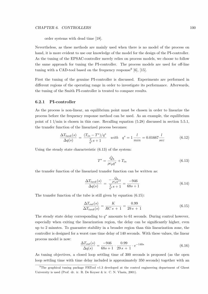
CHAPTER 6. CONTROLLERS 100
order systems with dead time [18].
Nevertheless, as these methods are mainly used when there is no model of the process onhand, it is more evident to use our knowledge of the model for the design of the PI-controller.As the tuning of the EPSAC-controller merely relies on process models, we choose to followthe same approach for tuning the PI-controller. The process models are used for off-linetuning with a CAD-tool based on the frequency response9 [6], [15].
First the tuning of the genuine PI-controller is discussed. Experiments are performed indifferent regions of the operating range in order to investigate its performance. Afterwards,the tuning of the Smith PI-controller is treated to compare results.
6.2.1 PI-controller
As the process is non-linear, an equilibrium point must be chosen in order to linearize theprocess before the frequency response method can be used. As an example, the equilibriumpoint of 1 l/min is chosen in this case. Recalling equation (5.28) discussed in section 5.5.1,the transfer function of the linearized process becomes:
∆Ttank(s)∆q(s)
=(Tin − T ∗)/q∗
Vq∗ s + 1
with q∗ = 1l
min= 0.01667
l
sec(6.12)
Using the steady state characteristic (6.13) of the system:
T ∗ =Qh
ρcpq∗+ Tin (6.13)
the transfer function of the linearized transfer function can be written as:
∆Ttank(s)∆q(s)
=− Qh
ρcpq∗2
Vq∗ s + 1
=−946
68s + 1(6.14)
The transfer function of the tube is still given by equation (6.15):
∆Tout(s)∆Ttank(s)
=K
RC s + 1=
0.9929 s + 1
(6.15)
The steady state delay corresponding to q∗ amounts to 61 seconds. During control however,especially when exiting the linearization region, the delay can be significantly higher, evenup to 2 minutes. To guarantee stability in a broader region than this linearization zone, thecontroller is designed for a worst case time delay of 140 seconds. With these values, the linearprocess model is now:
∆Tout(s)∆q(s)
=−946
68s + 1· 0.9929 s + 1
· e−140s (6.16)
As tuning objectives, a closed loop settling time of 300 seconds is proposed (as the openloop settling time with time delay included is approximately 350 seconds) together with an
9The graphical tuning package FRTool v1.3 developed at the control engineering department of Ghent
University is used (Prof. dr. ir. R. De Keyser & ir. C. N. Vlasin, 2001).
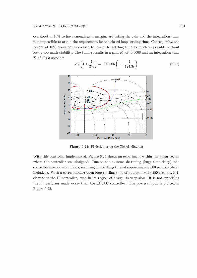
CHAPTER 6. CONTROLLERS 101
overshoot of 10% to have enough gain margin. Adjusting the gain and the integration time,it is impossible to attain the requirement for the closed loop settling time. Consequenlty, theborder of 10% overshoot is crossed to lower the settling time as much as possible withoutlosing too much stability. The tuning results in a gain Kc of -0.0006 and an integration timeTi of 124.3 seconds:
Kc
(1 +
1Tis
)= −0.0006
(1 +
1124.3s
)(6.17)
Figure 6.23: PI-design using the Nichols diagram
With this controller implemented, Figure 6.24 shows an experiment within the linear regionwhere the controller was designed. Due to the extreme de-tuning (huge time delay), thecontroller reacts overcautious, resulting in a settling time of approximately 600 seconds (delayincluded). With a corresponding open loop settling time of approximately 350 seconds, it isclear that the PI-controller, even in its region of design, is very slow. It is not surprisingthat it performs much worse than the EPSAC controller. The process input is plotted inFigure 6.25.
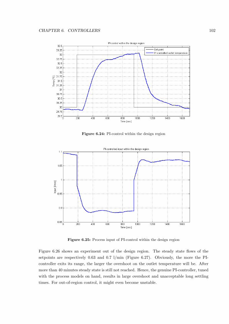
CHAPTER 6. CONTROLLERS 102
Figure 6.24: PI-control within the design region
Figure 6.25: Process input of PI-control within the design region
Figure 6.26 shows an experiment out of the design region. The steady state flows of thesetpoints are respectively 0.63 and 0.7 l/min (Figure 6.27). Obviously, the more the PI-controller exits its range, the larger the overshoot on the outlet temperature will be. Aftermore than 40 minutes steady state is still not reached. Hence, the genuine PI-controller, tunedwith the process models on hand, results in large overshoot and unacceptable long settlingtimes. For out-of-region control, it might even become unstable.
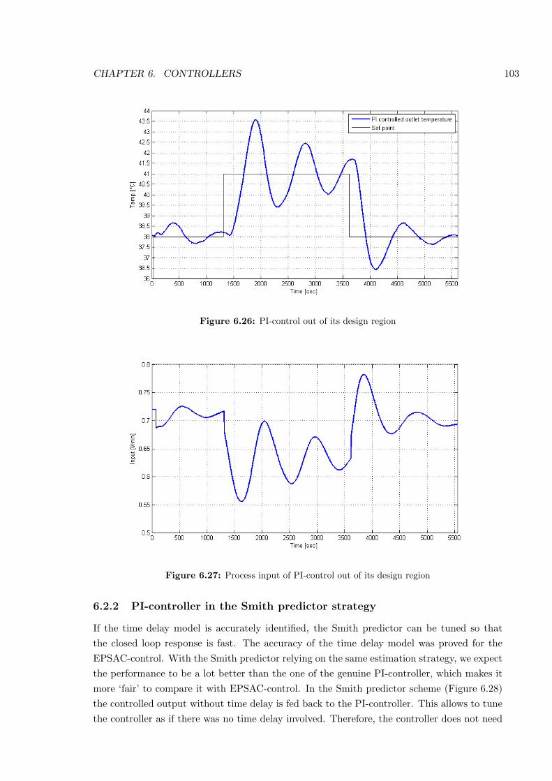
CHAPTER 6. CONTROLLERS 103
Figure 6.26: PI-control out of its design region
Figure 6.27: Process input of PI-control out of its design region
6.2.2 PI-controller in the Smith predictor strategy
If the time delay model is accurately identified, the Smith predictor can be tuned so thatthe closed loop response is fast. The accuracy of the time delay model was proved for theEPSAC-control. With the Smith predictor relying on the same estimation strategy, we expectthe performance to be a lot better than the one of the genuine PI-controller, which makes itmore ‘fair’ to compare it with EPSAC-control. In the Smith predictor scheme (Figure 6.28)the controlled output without time delay is fed back to the PI-controller. This allows to tunethe controller as if there was no time delay involved. Therefore, the controller does not need
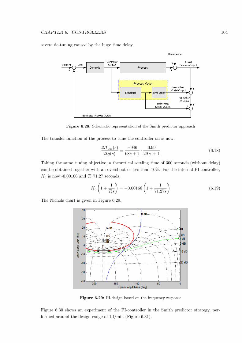
CHAPTER 6. CONTROLLERS 104
severe de-tuning caused by the huge time delay.
Figure 6.28: Schematic representation of the Smith predictor approach
The transfer function of the process to tune the controller on is now:
∆Tout(s)∆q(s)
=−946
68s + 1· 0.9929 s + 1
(6.18)
Taking the same tuning objective, a theoretical settling time of 300 seconds (without delay)can be obtained together with an overshoot of less than 10%. For the internal PI-controller,Kc is now -0.00166 and Ti 71.27 seconds:
Kc
(1 +
1Tis
)= −0.00166
(1 +
171.27s
)(6.19)
The Nichols chart is given in Figure 6.29.
Figure 6.29: PI-design based on the frequency response
Figure 6.30 shows an experiment of the PI-controller in the Smith predictor strategy, per-formed around the design range of 1 l/min (Figure 6.31).
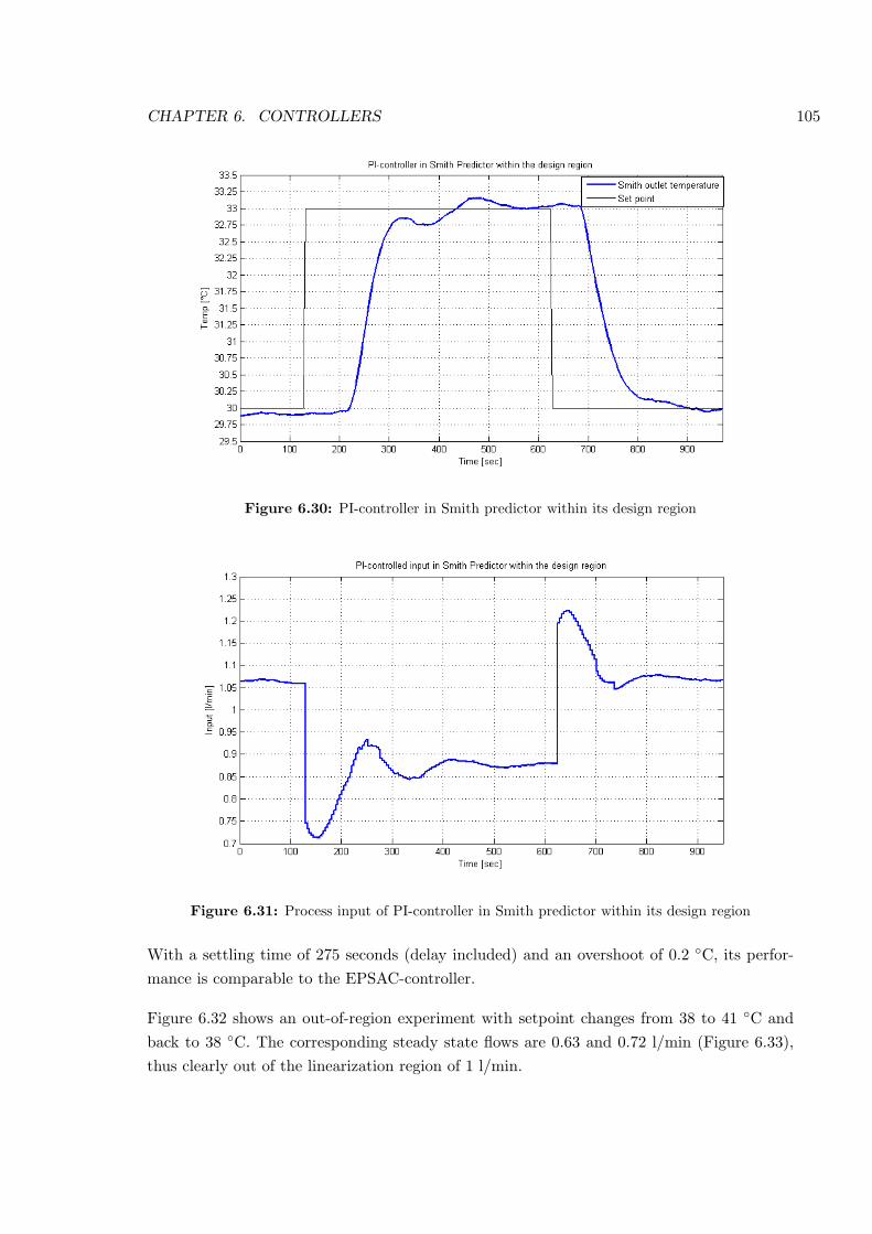
CHAPTER 6. CONTROLLERS 105
Figure 6.30: PI-controller in Smith predictor within its design region
Figure 6.31: Process input of PI-controller in Smith predictor within its design region
With a settling time of 275 seconds (delay included) and an overshoot of 0.2 C, its perfor-mance is comparable to the EPSAC-controller.
Figure 6.32 shows an out-of-region experiment with setpoint changes from 38 to 41 C andback to 38 C. The corresponding steady state flows are 0.63 and 0.72 l/min (Figure 6.33),thus clearly out of the linearization region of 1 l/min.
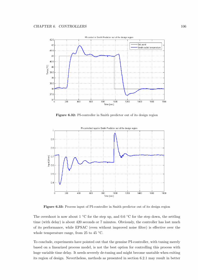
CHAPTER 6. CONTROLLERS 106
Figure 6.32: PI-controller in Smith predictor out of its design region
Figure 6.33: Process input of PI-controller in Smith predictor out of its design region
The overshoot is now about 1 C for the step up, and 0.6 C for the step down, the settlingtime (with delay) is about 420 seconds or 7 minutes. Obviously, the controller has lost muchof its performance, while EPSAC (even without improved noise filter) is effective over thewhole temperature range, from 25 to 45 C.
To conclude, experiments have pointed out that the genuine PI-controller, with tuning merelybased on a linearized process model, is not the best option for controlling this process withhuge variable time delay. It needs severely de-tuning and might become unstable when exitingits region of design. Nevertheless, methods as presented in section 6.2.1 may result in better
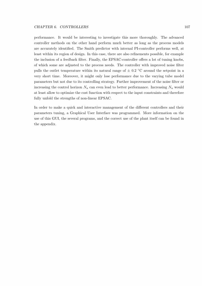
CHAPTER 6. CONTROLLERS 107
performance. It would be interesting to investigate this more thoroughly. The advancedcontroller methods on the other hand perform much better as long as the process modelsare accurately identified. The Smith predictor with internal PI-controller performs well, atleast within its region of design. In this case, there are also refinements possible, for examplethe inclusion of a feedback filter. Finally, the EPSAC-controller offers a lot of tuning knobs,of which some are adjusted to the process needs. The controller with improved noise filterpulls the outlet temperature within its natural range of ± 0.2 C around the setpoint in avery short time. Moreover, it might only lose performance due to the varying tube modelparameters but not due to its controlling strategy. Further improvement of the noise filter orincreasing the control horizon Nu can even lead to better performance. Increasing Nu wouldat least allow to optimize the cost function with respect to the input constraints and thereforefully unfold the strengths of non-linear EPSAC.
In order to make a quick and interactive management of the different controllers and theirparameters tuning, a Graphical User Interface was programmed. More information on theuse of this GUI, the several programs, and the correct use of the plant itself can be found inthe appendix.
Chapter 7
Conclusions
Having come to the end of this thesis, it is time to summarize a few realizations, conclusionsand proposals for further research.
7.1 The setup
The setup has been built and is operating well. Due to a good choice of the several parametersinvolved, the requirements for the process itself have been fullfilled:
1. A unit change in the input produces a significant change in the output.
2. The closed loop time constant equals roughly one minute.
3. The time constant of the tank is more or less equal to the transport delay.
A steep static characteristic explains the output sensitivity to input changes, while the choiceof a small tank volume and a high heat input, combined with a broad flow range results in afast response time. The transport delay is of the same order of magnitude as the tank timeconstant, as the volumes of the tank and the tube are 1.13 and 1.02 liter respectively. Abroad operational temperature range of approximately 12 C is reached.
A constant water level is obtained in a cheap and simple, but yet effective way via themechanical float switch. If the supply pressure of the tap water is sufficient, flows of up to 2l/min can be applied without causing the water level to decrease. The choice of a float switchallows to use an open tank, which makes it easy to put other elements like the heater, themixer and sensors inside the tank.
Using a peristaltic pump, a very accurate flow control is obtained, which is necessary fora precise temperature control. Besides its accuracy and fine resolution, it allows to makereliable calculations of the flow, which is very important in the calculation of the variabletime delay. This is possible due to the linear relation between the pump speed and the flow.The pump speed itself can not be measured easily, but this problem is solved by controllingthe DC-motor of the pump with a drive which has IxR feedforward compensation. Due tothis feature an almost linear relation between the control voltage to the drive and the pump
108
CHAPTER 7. CONCLUSIONS 109
speed is achieved, and, consequently, a linear relation between the control voltage and theflow can be assumed with a high reliability. Another advantage of the IxR compensation isthat changes in the setup (e.g. putting an outlet tube of different length) would not affect thelinear relation between control voltage and flow, although the load would have been changed.
A suitable data acquisition board was chosen, insuring measurements with a sufficient reso-lution. The board is provided with enough in- and outputs for the several measurements andthe flow control. More ports are available if one would consider further extensions.
Reliable Pt100 temperature sensors take care of the temperature registration. The circuitry toconvert the signals into a useful voltage range between 0 and 10 V is soldered. Investigationsand precautions have been taken thereby to insure measurements that are as accurate aspossible. Noise on the signals is filtered out via a passive RC filter combined with a digitalfilter on the computer. Finally, a calibration of the signals has been carried out in order toachieve reliable results.
All the electrical and electronic parts are put in a sealed box, separated from the water circuit.Switches for the different devices (pump, heater, mixer, main switch) are provided. All cablesand wires are placed in electrical wire grooves for protection and a neat arrangement.The water tank is made of plexiglass, which makes the process a bit more transparent andinteractive. Flexible plastic hoses are used for the in- and outlet tube. The 9.5 meters longoutlet tube is insulated, and curled up in a box. An easy attachment system to the watermains is provided.
7.2 Advanced Control
Regarding the EPSAC-based controller, first models of the several parts were derived andvalidated against experimental results. It turned out that the non-linear first order modelof the tank is very accurate, while the tube dynamics are in reality very complex. A linearfirst order approximation was used for it, and proved to give acceptable results, although farfrom ideal. Last but not least a model for the variable time delay was deduced, which wasrefined to compensate for the sensor reaction time. It is important for the controller that thiscalculation of the time delay is very precise, as an error of only one or two samples causesdifferences between the estimation of the current model output and the real process output.
The difficulties caused by the varying time delay were discussed (prediction of future timedelays, skipping samples or holding the same estimation over more samples, varying N1), andan appropriate strategy (based on the Smith predictor scheme) to deal with it was proposedand implemented.
The influence and importance of parameters like the prediction horizon N2 and the number ofiterations Ni has been examined. It turned out that N2 ·Ts should be a reasonable fraction ofthe (highest) time constant. Ni seems not to have a very important influence, but this is dueto the limited non-linearity within a limited temperature range. When ubase of EPSAC was
CHAPTER 7. CONCLUSIONS 110
compared to the one iterated by NEPSAC, it became clear that there was no much differencebetween the two, and hence, the influence of Ni remained small.
A first improvement of the noise model compared to the default one was implemented, andproved already its effectiveness. With this, the closed loop time constant of approximately1 minute is almost reached, while the overshoot remains very small.
As a reference, a genuine PI-controller and a PI-controller in the Smith predictor strategywere also implemented. It was shown that the genuine PI-controller, tuned with the processmodels on hand, needed severely de-tuning. Even then, it showed the tendency to becomeunstable when being operated out of the linearization region. The Smith predictor on theother hand can be classified as an advanced control method, which makes it a lot more suitableto control the heating tank system. It performed well for setpoint changes within its regionof design, but showed large overshoot when exiting it.Finally, a Graphical User Interface was programmed to make experimenting and switchingbetween the different controllers easier and more accessible.
Although very promising results are obtained, there are still a lot of interesting options leftfor further research and improvement. The ones we have in mind are summarized briefly.
• Probably the most expectant topic to be further examined is the model of the tube.Maybe a better but still simple model can be derived. The first thing that can be triedconcerning this problem is making the parameters of the transfer function adaptive tothe flow and/or temperature. In this way it should be possible to obtain a more reliabletube model, resulting in a better control. It also turned out that a correct estimationof the time delay is extremely important for a good control. As the conversion factorbetween control voltage and flow might change slightly depending on the temperatureof the pump motor (due to the not ideal IxR feedforward compensation, see section3.1.2) it is possible that there is an error of ± 5 seconds. Maybe a more steady motortemperature can be achieved by providing an efficient heat removal using heat sinks ora fan.
• Another promising feature is the noise model. A first improvement compared to thedefault noise model has been implemented, but it is certainly useful to investigate morecomplex models, resulting for example in a low pass filter with a very small cut-offfrequency and a very steep slope.
• Something that is not yet investigated is the shape of the reference trajectory. In allexperiments described in this thesis a step reference was used, while choosing a smoothertransition could result in a control output with for example less overshoot.
• Another possibility lies in the control horizon Nu, which has been chosen equal to 1 uptill now. Although this choice causes a profound simplification and has proved goodresults, there are some disadvantages: clipping is the only option as there are no other
CHAPTER 7. CONCLUSIONS 111
degrees of freedom to calculate the optimal input with respect to input constraints.Especially when making large setpoint steps, a clipping situation is very likely to occur.
• An attempt can be made to use the (N)EPSAC-algorithm without the decoupling of thevariable time delay from the dynamics. As explained complex problems and calculationscan however be expected if the theory is strictly applied. But it is always possible thatsome simplifying assumptions (for instance not predicting the future time delay, buttaking it equal to the current delay) could lead to good results.
Besides the EPSAC-method, also other controllers can be tried or improved. As the PI-controller in the Smith predictor scheme showed good results within its linearization region,it could be useful to split up the whole temperature range and to design for each separaterange an appropriate PI-controller. Then the parameters of the PI-controller can be madeadaptive depending on the current temperature (e.g. by interpolation between the parametersof the several designs).
The plant itself could also be extended with features which can make the heat input forinstance manipulable (e.g. via a dimmer). In this way the plant could also be used as atest setup for problems with a constant time delay (e.g. a constant pump speed with amanipulated heat input). As an ultimate bonus, by manipulating both the pump and theheater, the setup could also be used as a MIMO1 system (with variable time delay), whichwould pose another very challenging research topic.
Starting with these suggestions, it is clear that quite a lot of further research can be done onthis problem. A real setup is however available and working properly, while the difficultieswith a variable time delay are mapped out. The first steps have been made and alreadyresulted in a good control. Consequently, the most important conclusion that can be drawnfrom this thesis is that EPSAC - if applied in a proper way - has no problem at all in dealingwith real life processes with a variable time delay.
1Multiple Input Multiple Output
Appendix A
GUIDE
A.1 Introduction and Installation
This appendix serves as a manual on how to perform experiments on the heating tank systemin a safe way. It also guides the user through the implementation of the different self-tunedcontrollers classified as:
• a genuine PID-controller: Kp, Ti, Td
• a Smith predictor with internal PID-controller: Kp, Ti, Td
• a non-linear EPSAC controller: N2, Ni, a
The respective parameters form the heart of the controller and can be easily adapted in aGraphical User Interface (GUI). The GUI also serves to change the parameters of the dynamicmodels of the tank and the outlet tube and allows to redefine parameters which govern theexecution of the experiment (e.g. input constraints, sampling time).
The GUI organizes all files involved in controlling the heating tank system. NI-DAQ fromNational Instruments and the Matlab Data Acquisition Toolbox exchange the control andmeasurement signals between the GUI and the process. These packages together with theGUI and the control files can be installed from the CD which accompanies this thesis. Makesure these packages are properly installed before installing the GUI. Information can be foundin the readme.txt file. Once these packages are installed, select a directory and finish theinstallation by copying all GUI files to the directory. This includes all control files and thesupport files of the graphical user interfaces.
A.2 Control structure
The GUI control structure is shown in Figure A.1. This structure and its blocks are brieflydiscussed here. A detailed explanation is given in the following sections.STARTPROCESS allows to define general parameters that will be used during the experiment,for instance the parameters of the dynamic models. If these model parameters are changed,
112
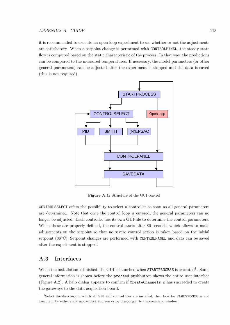
APPENDIX A. GUIDE 113
it is recommended to execute an open loop experiment to see whether or not the adjustmentsare satisfactory. When a setpoint change is performed with CONTROLPANEL, the steady stateflow is computed based on the static characteristic of the process. In that way, the predictionscan be compared to the measured temperatures. If necessary, the model parameters (or othergeneral parameters) can be adjusted after the experiment is stopped and the data is saved(this is not required).
Figure A.1: Structure of the GUI control
CONTROLSELECT offers the possibility to select a controller as soon as all general parametersare determined. Note that once the control loop is entered, the general parameters can nolonger be adjusted. Each controller has its own GUI-file to determine the control parameters.When these are properly defined, the control starts after 80 seconds, which allows to makeadjustments on the setpoint so that no severe control action is taken based on the initialsetpoint (38C). Setpoint changes are performed with CONTROLPANEL and data can be savedafter the experiment is stopped.
A.3 Interfaces
When the installation is finished, the GUI is launched when STARTPROCESS is executed1. Somegeneral information is shown before the proceed pushbutton shows the entire user interface(Figure A.2). A help dialog appears to confirm if CreateChannels.m has succeeded to createthe gateways to the data acquisition board.
1Select the directory in which all GUI and control files are installed, then look for STARTPROCESS.m and
execute it by either right mouse click and run or by dragging it to the command window.
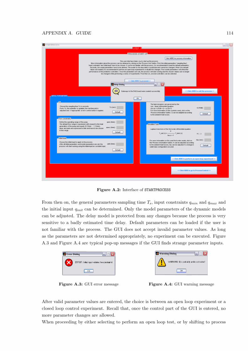
APPENDIX A. GUIDE 114
Figure A.2: Interface of STARTPROCESS
From then on, the general parameters sampling time Ts, input constraints qmin and qmax andthe initial input qinit can be determined. Only the model parameters of the dynamic modelscan be adjusted. The delay model is protected from any changes because the process is verysensitive to a badly estimated time delay. Default parameters can be loaded if the user isnot familiar with the process. The GUI does not accept invalid parameter values. As longas the parameters are not determined appropriately, no experiment can be executed. FigureA.3 and Figure A.4 are typical pop-up messages if the GUI finds strange parameter inputs.
Figure A.3: GUI error message Figure A.4: GUI warning message
After valid parameter values are entered, the choice is between an open loop experiment or aclosed loop control experiment. Recall that, once the control part of the GUI is entered, nomore parameter changes are allowed.When proceeding by either selecting to perform an open loop test, or by shifting to process
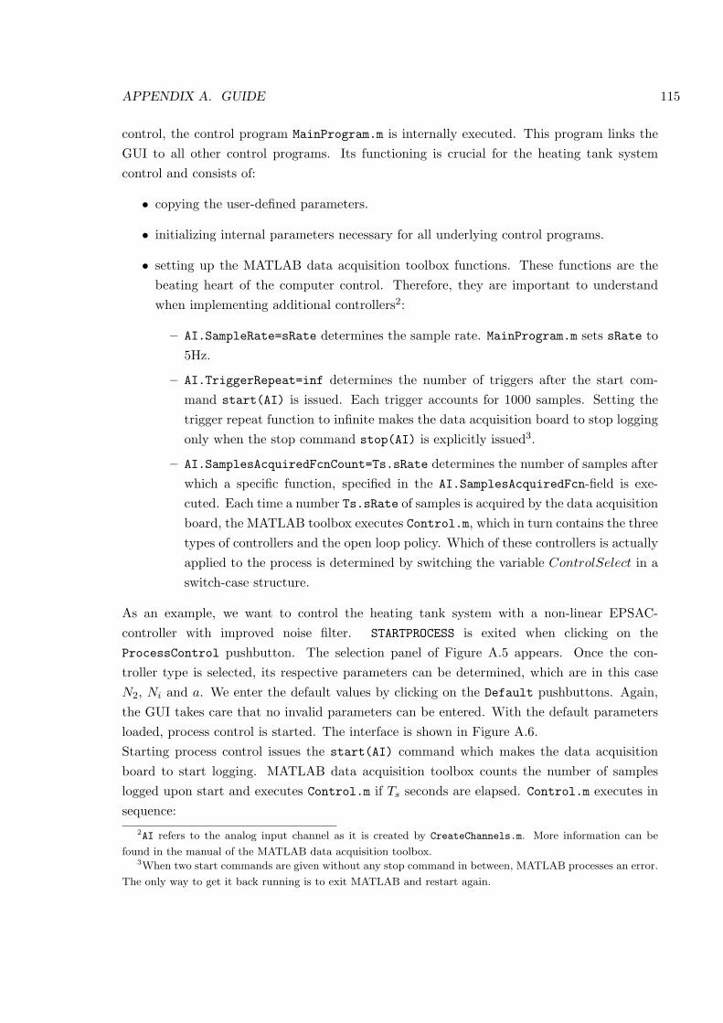
APPENDIX A. GUIDE 115
control, the control program MainProgram.m is internally executed. This program links theGUI to all other control programs. Its functioning is crucial for the heating tank systemcontrol and consists of:
• copying the user-defined parameters.
• initializing internal parameters necessary for all underlying control programs.
• setting up the MATLAB data acquisition toolbox functions. These functions are thebeating heart of the computer control. Therefore, they are important to understandwhen implementing additional controllers2:
– AI.SampleRate=sRate determines the sample rate. MainProgram.m sets sRate to5Hz.
– AI.TriggerRepeat=inf determines the number of triggers after the start com-mand start(AI) is issued. Each trigger accounts for 1000 samples. Setting thetrigger repeat function to infinite makes the data acquisition board to stop loggingonly when the stop command stop(AI) is explicitly issued3.
– AI.SamplesAcquiredFcnCount=Ts.sRate determines the number of samples afterwhich a specific function, specified in the AI.SamplesAcquiredFcn-field is exe-cuted. Each time a number Ts.sRate of samples is acquired by the data acquisitionboard, the MATLAB toolbox executes Control.m, which in turn contains the threetypes of controllers and the open loop policy. Which of these controllers is actuallyapplied to the process is determined by switching the variable ControlSelect in aswitch-case structure.
As an example, we want to control the heating tank system with a non-linear EPSAC-controller with improved noise filter. STARTPROCESS is exited when clicking on theProcessControl pushbutton. The selection panel of Figure A.5 appears. Once the con-troller type is selected, its respective parameters can be determined, which are in this caseN2, Ni and a. We enter the default values by clicking on the Default pushbuttons. Again,the GUI takes care that no invalid parameters can be entered. With the default parametersloaded, process control is started. The interface is shown in Figure A.6.Starting process control issues the start(AI) command which makes the data acquisitionboard to start logging. MATLAB data acquisition toolbox counts the number of sampleslogged upon start and executes Control.m if Ts seconds are elapsed. Control.m executes insequence:
2AI refers to the analog input channel as it is created by CreateChannels.m. More information can be
found in the manual of the MATLAB data acquisition toolbox.3When two start commands are given without any stop command in between, MATLAB processes an error.
The only way to get it back running is to exit MATLAB and restart again.
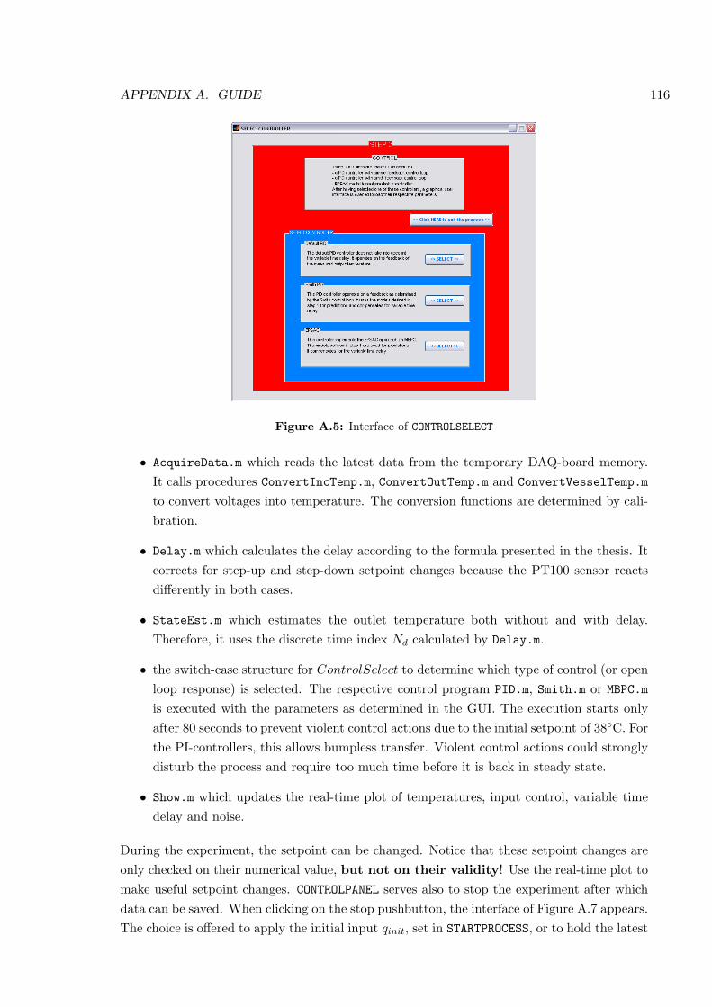
APPENDIX A. GUIDE 116
Figure A.5: Interface of CONTROLSELECT
• AcquireData.m which reads the latest data from the temporary DAQ-board memory.It calls procedures ConvertIncTemp.m, ConvertOutTemp.m and ConvertVesselTemp.m
to convert voltages into temperature. The conversion functions are determined by cali-bration.
• Delay.m which calculates the delay according to the formula presented in the thesis. Itcorrects for step-up and step-down setpoint changes because the PT100 sensor reactsdifferently in both cases.
• StateEst.m which estimates the outlet temperature both without and with delay.Therefore, it uses the discrete time index Nd calculated by Delay.m.
• the switch-case structure for ControlSelect to determine which type of control (or openloop response) is selected. The respective control program PID.m, Smith.m or MBPC.m
is executed with the parameters as determined in the GUI. The execution starts onlyafter 80 seconds to prevent violent control actions due to the initial setpoint of 38C. Forthe PI-controllers, this allows bumpless transfer. Violent control actions could stronglydisturb the process and require too much time before it is back in steady state.
• Show.m which updates the real-time plot of temperatures, input control, variable timedelay and noise.
During the experiment, the setpoint can be changed. Notice that these setpoint changes areonly checked on their numerical value, but not on their validity! Use the real-time plot tomake useful setpoint changes. CONTROLPANEL serves also to stop the experiment after whichdata can be saved. When clicking on the stop pushbutton, the interface of Figure A.7 appears.The choice is offered to apply the initial input qinit, set in STARTPROCESS, or to hold the latest
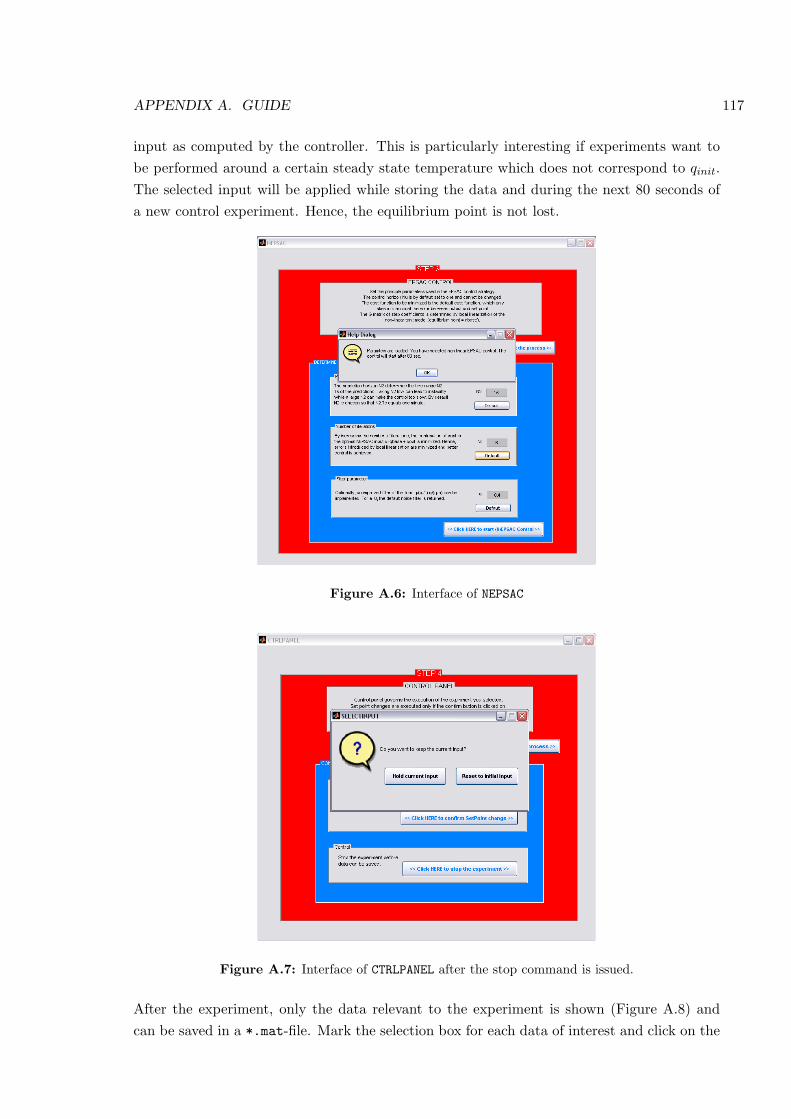
APPENDIX A. GUIDE 117
input as computed by the controller. This is particularly interesting if experiments want tobe performed around a certain steady state temperature which does not correspond to qinit.The selected input will be applied while storing the data and during the next 80 seconds ofa new control experiment. Hence, the equilibrium point is not lost.
Figure A.6: Interface of NEPSAC
Figure A.7: Interface of CTRLPANEL after the stop command is issued.
After the experiment, only the data relevant to the experiment is shown (Figure A.8) andcan be saved in a *.mat-file. Mark the selection box for each data of interest and click on the
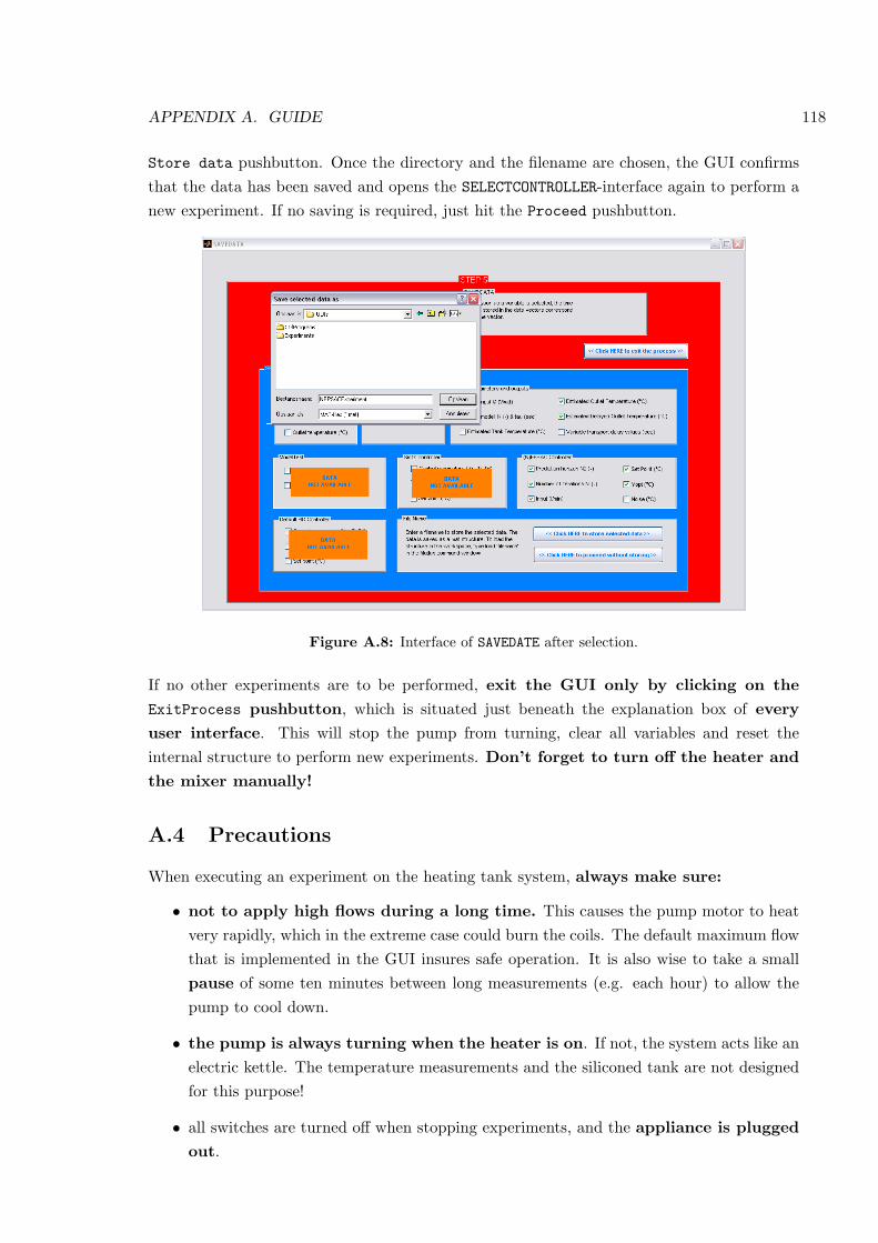
APPENDIX A. GUIDE 118
Store data pushbutton. Once the directory and the filename are chosen, the GUI confirmsthat the data has been saved and opens the SELECTCONTROLLER-interface again to perform anew experiment. If no saving is required, just hit the Proceed pushbutton.
Figure A.8: Interface of SAVEDATE after selection.
If no other experiments are to be performed, exit the GUI only by clicking on theExitProcess pushbutton, which is situated just beneath the explanation box of everyuser interface. This will stop the pump from turning, clear all variables and reset theinternal structure to perform new experiments. Don’t forget to turn off the heater andthe mixer manually!
A.4 Precautions
When executing an experiment on the heating tank system, always make sure:
• not to apply high flows during a long time. This causes the pump motor to heatvery rapidly, which in the extreme case could burn the coils. The default maximum flowthat is implemented in the GUI insures safe operation. It is also wise to take a smallpause of some ten minutes between long measurements (e.g. each hour) to allow thepump to cool down.
• the pump is always turning when the heater is on. If not, the system acts like anelectric kettle. The temperature measurements and the siliconed tank are not designedfor this purpose!
• all switches are turned off when stopping experiments, and the appliance is pluggedout.

APPENDIX A. GUIDE 119
• not to forget to close the water valve before leaving, as the float switch mightleak after some time. To avoid rusting of the mixer screw, the inlet tube should bedisconnected from the water mains to lower the water level below the mixer screw.Afterwards, the inlet tube can be connected again to avoid air coming into the tubes.
© Himpe Steven and Theunynck Vincent, academic year 2005-2006
List of Figures
1.1 Schematic representation of a steel rolling process . . . . . . . . . . . . . . . . 11.2 Schematic representation of the Smith predictor approach . . . . . . . . . . . 31.3 Schematic representation of the process . . . . . . . . . . . . . . . . . . . . . 4
2.1 Effect of a not tuned set of parameters on the operating range . . . . . . . . 102.2 Effect of a tuned set of parameters on the operating range . . . . . . . . . . . 112.3 Overflow system . . . . . . . . . . . . . . . . . . . . . . . . . . . . . . . . . . 122.4 Mounting of the temperature sensor in an overflow configuration . . . . . . . 122.5 Pressurized tank . . . . . . . . . . . . . . . . . . . . . . . . . . . . . . . . . . 132.6 Communicating vessels design . . . . . . . . . . . . . . . . . . . . . . . . . . . 142.7 Relay-guarded level . . . . . . . . . . . . . . . . . . . . . . . . . . . . . . . . . 152.8 Float switch guarded level . . . . . . . . . . . . . . . . . . . . . . . . . . . . . 162.9 Streamline for the Bernoulli equation . . . . . . . . . . . . . . . . . . . . . . . 172.10 Cross section enlargement at the fitting . . . . . . . . . . . . . . . . . . . . . 192.11 Curvature of the outlet tube . . . . . . . . . . . . . . . . . . . . . . . . . . . . 202.12 Comparison of results for D0 = 10mm . . . . . . . . . . . . . . . . . . . . . 222.13 Comparison of results for D0 = 15mm . . . . . . . . . . . . . . . . . . . . . 232.14 Variables of interest . . . . . . . . . . . . . . . . . . . . . . . . . . . . . . . . 24
3.1 Influence of IxR compensation on the linearity of flow control. . . . . . . . . . 313.2 DC-sources for temperature measurement . . . . . . . . . . . . . . . . . . . . 323.3 The National Instruments USB-6008 Data Acquistion Board . . . . . . . . . 333.4 Internal flow in the tank . . . . . . . . . . . . . . . . . . . . . . . . . . . . . . 353.5 Electric scheme of the setup . . . . . . . . . . . . . . . . . . . . . . . . . . . . 363.6 Protection of electric devices in the setup . . . . . . . . . . . . . . . . . . . . 373.7 Peristaltic pump . . . . . . . . . . . . . . . . . . . . . . . . . . . . . . . . . . 383.8 Fully insulated outlet tube . . . . . . . . . . . . . . . . . . . . . . . . . . . . . 383.9 Overview of the entire plant . . . . . . . . . . . . . . . . . . . . . . . . . . . . 39
4.1 Thermocouple . . . . . . . . . . . . . . . . . . . . . . . . . . . . . . . . . . . . 414.2 Comparison of characteristics . . . . . . . . . . . . . . . . . . . . . . . . . . . 424.3 Resistance-Temperature Characteristic of Pt100 . . . . . . . . . . . . . . . . . 434.4 Fixed Current Excitation . . . . . . . . . . . . . . . . . . . . . . . . . . . . . 45
120
LIST OF FIGURES 121
4.5 The Wheatstone bridge . . . . . . . . . . . . . . . . . . . . . . . . . . . . . . 464.6 Characteristic Wheatstone bridge & Amplifier . . . . . . . . . . . . . . . . . . 474.7 Scheme Differential Amplifier . . . . . . . . . . . . . . . . . . . . . . . . . . . 474.8 Scheme Instrumentation Amplifier . . . . . . . . . . . . . . . . . . . . . . . . 494.9 A typical first measurement . . . . . . . . . . . . . . . . . . . . . . . . . . . . 514.10 Noise Spectrum . . . . . . . . . . . . . . . . . . . . . . . . . . . . . . . . . . . 524.11 Measurement after filtering at 6 Hz . . . . . . . . . . . . . . . . . . . . . . . . 524.12 Noise spectrum after filtering at 6 Hz . . . . . . . . . . . . . . . . . . . . . . . 534.13 Noise spectra after filtering at 6 Hz for different pump speeds . . . . . . . . . 534.14 Lowpass filter with cutoff frequency of 1.1 Hz . . . . . . . . . . . . . . . . . . 544.15 Measurement after filtering at 1.1 Hz . . . . . . . . . . . . . . . . . . . . . . . 554.16 Temperature conversion schematics . . . . . . . . . . . . . . . . . . . . . . . . 554.17 Accuracy of temperature conversion . . . . . . . . . . . . . . . . . . . . . . . 574.18 Calibration of the inlet water temperature . . . . . . . . . . . . . . . . . . . 574.19 Calibration of the outlet water temperature . . . . . . . . . . . . . . . . . . . 58
5.1 Control volume of the tank for the energy balance . . . . . . . . . . . . . . . 615.2 Tank and outlet temperature as functions of the flow (tube without insulation) 655.3 Heat loss as function of flow for insulated and non-insulated tube . . . . . . . 665.4 Tank and Outlet Temperature as function of the flow, insulated tube . . . . . 675.5 Finite element grid of the insulated tube . . . . . . . . . . . . . . . . . . . . . 675.6 Insulated tube with simplified temperature distribution . . . . . . . . . . . . 685.7 Position at each sampling time of the mass particle flowing through the outlet
tube . . . . . . . . . . . . . . . . . . . . . . . . . . . . . . . . . . . . . . . . . 705.8 Definition time delay . . . . . . . . . . . . . . . . . . . . . . . . . . . . . . . . 715.9 Step response . . . . . . . . . . . . . . . . . . . . . . . . . . . . . . . . . . . . 735.10 Experimental versus theoretical time constants . . . . . . . . . . . . . . . . . 745.11 Experimental versus theoretical static gains . . . . . . . . . . . . . . . . . . . 745.12 Tank model validation . . . . . . . . . . . . . . . . . . . . . . . . . . . . . . . 755.13 Static Gain of the outlet tube for heating and cooling . . . . . . . . . . . . . 765.14 Tube model validation . . . . . . . . . . . . . . . . . . . . . . . . . . . . . . . 76
6.1 EPSAC control concept for Nu = 1 . . . . . . . . . . . . . . . . . . . . . . . . 806.2 Parallel model implementation . . . . . . . . . . . . . . . . . . . . . . . . . . 826.3 Estimation procedure for the outlet temperature . . . . . . . . . . . . . . . . 836.4 Example of the discrete time delay evolution according to (5.24) . . . . . . . 846.5 Prediction procedure of the outlet temperature . . . . . . . . . . . . . . . . . 866.6 Snapshots of the future outlet temperature profile at different sampling instants 876.7 Control loop layout of the heating tank system . . . . . . . . . . . . . . . . . 886.8 Effect of different N2 on the controller performance . . . . . . . . . . . . . . . 906.9 Process input for different N2 . . . . . . . . . . . . . . . . . . . . . . . . . . . 906.10 Evolution of gN2 · δuopt for different Ni . . . . . . . . . . . . . . . . . . . . . . 92
LIST OF FIGURES 122
6.11 Controlled outlet temperature for different Ni . . . . . . . . . . . . . . . . . . 936.12 Static characteristic of the tank . . . . . . . . . . . . . . . . . . . . . . . . . . 936.13 Computed input for different Ni . . . . . . . . . . . . . . . . . . . . . . . . . 936.14 Setpoint changes over the entire temperature region . . . . . . . . . . . . . . 946.15 Estimation of the outlet temperature in different parts of the range . . . . . . 956.16 Setpoint change in the most non-linear zone of the system . . . . . . . . . . . 966.17 Inputs for a setpoint change in the most non-linear zone of the system . . . . 966.18 Noise evolution . . . . . . . . . . . . . . . . . . . . . . . . . . . . . . . . . . . 976.19 Noise spectrum . . . . . . . . . . . . . . . . . . . . . . . . . . . . . . . . . . . 976.20 Bode diagram of the improved noise filter . . . . . . . . . . . . . . . . . . . . 986.21 Controller performance with improved noise filter . . . . . . . . . . . . . . . . 986.22 Process input with default and improved noise filter . . . . . . . . . . . . . . 996.23 PI-design using the Nichols diagram . . . . . . . . . . . . . . . . . . . . . . . 1016.24 PI-control within the design region . . . . . . . . . . . . . . . . . . . . . . . . 1026.25 Process input of PI-control within the design region . . . . . . . . . . . . . . 1026.26 PI-control out of its design region . . . . . . . . . . . . . . . . . . . . . . . . . 1036.27 Process input of PI-control out of its design region . . . . . . . . . . . . . . . 1036.28 Schematic representation of the Smith predictor approach . . . . . . . . . . . 1046.29 PI-design based on the frequency response . . . . . . . . . . . . . . . . . . . . 1046.30 PI-controller in Smith predictor within its design region . . . . . . . . . . . . 1056.31 Process input of PI-controller in Smith predictor within its design region . . . 1056.32 PI-controller in Smith predictor out of its design region . . . . . . . . . . . . 1066.33 Process input of PI-controller in Smith predictor out of its design region . . . 106
A.1 Structure of the GUI control . . . . . . . . . . . . . . . . . . . . . . . . . . . 113A.2 Interface of STARTPROCESS . . . . . . . . . . . . . . . . . . . . . . . . . . . . . 114A.3 GUI error message . . . . . . . . . . . . . . . . . . . . . . . . . . . . . . . . . 114A.4 GUI warning message . . . . . . . . . . . . . . . . . . . . . . . . . . . . . . . 114A.5 Interface of CONTROLSELECT . . . . . . . . . . . . . . . . . . . . . . . . . . . . 116A.6 Interface of NEPSAC . . . . . . . . . . . . . . . . . . . . . . . . . . . . . . . . . 117A.7 Interface of CTRLPANEL after the stop command is issued. . . . . . . . . . . . 117A.8 Interface of SAVEDATE after selection. . . . . . . . . . . . . . . . . . . . . . . . 118
Bibliography
[1] J. Barraud, Y. Creff, and N. Petit. PI controllers performances for a process model withvarying delay. A Diesel Hydrodesulfurization process.
[2] W. Bolton. Mechatronics, 3rd Edition. Pearson Education Limited, 2003.
[3] E.F. Camacho and C. Bordons. Model Predictive Control. Springer-Verlag, 1999.
[4] G.H. Cohen and G.A. Coon. Theoretical consideration of retarded control. Trans. ASME,75:827–834, 1953.
[5] S. Cristea, C. de Prada, and R. De Keyser. Predictive Control of a Process with VariableDead-Time. Preprints of the 16th IFAC World Congress, Prague, 4-8 July 2005.
[6] R. De Keyser. Computersturing van industriele processen, course notes Ghent University,Department of Electrical Energy, Systems and Automation, Academic year 2004-2005.
[7] R. De Keyser. A ‘Gent’le Approach to Predictive Control. UNESCO Encyclopaedia ofLife Support Systems (EoLSS), 2003.
[8] A. Van den Bossche and W. De Waele. Technologie en Veiligheid van Elektrische enMechanische Installaties, course notes Ghent University, Academic year 2005-2006.
[9] E. Dick. Turbomachines, course notes Ghent University, Department of Flow, Heat andCombustion mechanics, Academic year 2003-2004.
[10] C.C. Hang, K.J. Astrom, and W.K. Ho. Refinements of the Ziegler-Nichols tuning for-mulas. IEE Proceeding-D, 138:111–118, 1991.
[11] I.E. Idelchik. Handbook of Hydraulic Resistance, 3rd edition. CRC Press, 1993.
[12] B.P. Lathi. Signal Processing & Linear Systems. Oxford University Press, 1998.
[13] J. Melkebeek. Gestuurde Elektrische Aandrijvingen, course notes Ghent University, De-partment of Electrical Energy, Systems and Automation, Academic year 2004-2005.
[14] M.J. Moran and H.N. Shapiro. Fundamentals of Engineering Thermodynamics, 3rd Edi-tion. John Wiley & Sons, 1998.
[15] N.S. Nise. Control Systems Engineering, third edition. John Wiley & Sons, 2000.
123
BIBLIOGRAPHY 124
[16] R. Sierens. Zuigermachines, course notes Ghent University, Department of Flow, Heatand Combustion mechanics, Academic year 2004-2005.
[17] O.J.M. Smith. Closer Control of Loops with Dead Time. Chemical Engineering Progress,53:217–219, 1957.
[18] S. Tavakoli and P. Fleming. Optimal tuning of PI controllers for first order plus deadtime / long dead time models using dimensional analysis. In Proc. of the 7th EuropeanControl Conf., 2003.
[19] Temperatures.com, Inc. About Temperature Sensors. http://www.temperatures.com.
[20] A. Van Calster. Elektronische Systemen en Instrumentatie, course notes Ghent Univer-sity, Department of Electronics and Information Systems, Academic year 2002-2003.
[21] A. Van Calster. Industrieel Elektrische Meting, course notes Ghent University, Depart-ment of Electronics and Information Systems, Academic year 2005-2006.
[22] P. Vandevelde. Warmte- en Verbrandingstechniek, course notes Ghent University, De-partment of Flow, Heat and Combustion mechanics, Academic year 2003-2004.
[23] J.R. Welty, Ch.E. Wicks, R.E. Wilson, and G. Rorrer. Fundamentals of Momentum,Heat, and Mass Transfer, 4th Edition. John Wiley & Sons, 2001.
[24] J.G. Ziegler and N.B. Nichols. Optimum Settings for Automatic Controllers. Trans.ASME, 64:759–768, 1942.