Embed Size (px)
Citation preview

DESIGN OF A GAS HOLDUP SENSOR FOR FLOTATION DIAGNOSIS
DEPARTMENT OF MIN~NG AND METALLURGICAL ENG~NEERING
MCGILL UNIVERSITY
MONTREAL, CANADA
AUGUST, 1998
A TiiESiS SL~B~IITTEDTO THE FACULTY OF
GRADUATE SI-UDIES AND RESEARCH
IN PARTIAL FULFlLLhlENT OF Tt IE REQUiREMENTS OF THE DEGREE OF
MASTER OF ENGINEERING

I I
National Library l
BiMiothéque nationale du Canada
Acquisitions and Acquisitions et Bibliographie Services services bibliographiques
The author has granted a non- exclusive licence ailowing the National Library of Canada to reproduce, loan, distribute or seU copies of this thesis in microfom, paper or electronic formats.
The author retains ownership of the copyright in this thesis. Neither the thesis nor substantiai extracts fiom it may be printed or otherwise reproduced without the author's permission.
L'auteur a accordé une licence non exclusive permettant à la Bibliothèque nationale du Canada de reproduire, prêter, distribuer ou vendre des copies de cette thèse sous la fonne de microfiche/nlm, de reproduction sur papier ou sur format électronique.
L'auteur conserve la propriété du droit d'auteur qui protège cette thèse. Ni la thèse ni des extraits substantiels de celle-ci ne doivent être imprimés ou autrement reproduits sans son autorisation.

This fhesis is dediccred !O my wife Karen
And my son Javier who is leurning #O live

The mineral processing group of McGill University developed a novel gas
holdup probe that consists of two conductivity flow cells: an open ce11 used
to estimate dispersion (sluny + air) conductivity and a syphon ce11 used to
estimate sluny conductivity. These two values are entered into Maxwell's
mode1 to calculate gas holdup.
In this work some design criteria for conductivity flow celis and the syphon
ce11 are given. Effect of geometrical ceil constant and electrode width on
ce11 behaviour are analyzed. New dimensions for open and syphon cells are
proposed. Conditions to prevent bubbles from being entrained into the
syphon cell are established.
The new design of the gas holdup probe was tested successfully over a
prolonged period at the INCO Matte Separation Plant (Copper Cliff,
Ontario). Tests carried out in waste paper de-inking at BOWATER
(Gatineau, Quebec) showed ihc gas holdup va
with the values obtained froni prcssurc. The
holdup signal obtaincd by thc prohc could
operation.
lues given by the probe agreed
noise associated with the gas
be used to diagnose sparger
Gas holdup showed some degree of correlation with notation efficiency of
waste paper de-inking and tlotation rate constant. Chemistry and rheology of
the feed are other factors to be considered. Estimation of bubble surface area
flux should consider rheology properties (liquid viscosity and density).

Le groupe de procédés des minerais de l'université McGill a développé une
nouvelle sonde de fraction gazeuse qui consiste en deux cellules de
conductibilité du débit: une cellule ouverte, utilisée dans l'estimation de la
conductibilité de la dispersion (pulpe + air), et une cellule siphon, utilisée
dans l'estimation de la conductibilité de la pulpe. Ces deux valeurs entrent
dans le modèle de Maxwell utilisé, afin de calculer la fraction gazeuse.
Dans ce travail, quelques critères de design pour des cellules de
conductibilité du débit, et la cellule siphon, sont donnés. Les effets de la
constante géométrique de la cellule et de la largeur de l'électrode sur le
comporiement de la cellule sont analysés. De nouvelles dimensions pour des
cellules ouverte et siphon sont proposées. Des conditions de prévention
d'entraînement des bulles dans la cellule siphon sont établies.
Le nouveau design de la sonde de fraction gazeuse a été testé avec succès,
sur une période prolongée, à l'usine INCO Matte Separation Plant (Copper
Cliff. Ontario). Les tests effectués dans le désencrage de papier recyclé à
BOWATER (Gatineau, Québec) ont démontré que les valeurs de fraction
eazeuse obtenues par la sonde étaient en accord avec les valeurs obtenues b
des mesures de pression. L'interférence associée au signal de fraction
gazeuse obtenu par la sonde pourrait être utilisée dans le diagnostic
d'opération du barboteur.
La fraction gazeuse a démontré un certain degre de corrélation avec le
rendement de flottation du désencrage du papier recyclé et la constante du

taux de flottation. La chimie et la théologie de l'alimentation sont d'autres
facteurs à considérar. L'estimation du flux de surface des bulles devrait tenir
compte des propriktés rhéologiques (viscosité et densité du liquide).

1 would like to thank my supervisor, Professor J.A. Finch and Dr. C.O.
Gomez for their invaluable contributions and support of my work,
especially, for the opportunity of participating in the McGill mineral
processing group.
Also, 1 want to thank al1 members of the sensor/column flotation group at
McGilI University, and specialiy Mr. H. Hemindez, Dr. R. Escudero, Dr. F.
Tavera, Mr. G. Leichtle and Mr. C. Hardie for a most pleasant working
atmosphere.
1 want to express my gratitude to Mr. R. Agnew and Mr. C. Pollard for their
constant support during the plant tests and al1 the staff and crew of the
Matte Separation Plant, INCO ltd.
Finally, I want to thank the staff and crew at the waste paper de-inking plant,
BOWATER Pulp and Paper Inc.

1.1. UNDERSTANDING THE PROBLEM
1.2. OBJECTIVES AND ORGANIZXT~ON OF THE THESIS
CHAPTER 2: BACKGROUND
2.1. DEFINITION OF CONDCCTIVITY
2.3. ~IEASCRISG COSDCCTI VITI'
2.3. MASWELL'S MODEL
2.4. COSDL'CTIVITI- FLOW CELLS
2.5. Gxs HOLDCP PROBE: ~ ~ C G I L L PROTOTYPE
2.6. PRISCIPLES OF Tt IE Sj'Pt IO\ CELL
2.7. DESCRIPTIOS OF FL-OTXTIO\ C'OLLSIX
2.8. EFFECT OF OPERATISG AXD DESICX VARIABLES OS GAS HOLDUP
2.8.1. OPERATING VARIABLES
2.8.2. DESIGS VARIABLES
2.9. GAS HOLDUP ROLE 1s FLOTATIOS PERFORMANCE
2.1 0. BUBBLE SURFACE AREh FLUX ESTIMATION

CHAPTER 3: DESIGN CRITERIA FOR GAS HOLDUP SENSOR
3.1. INTRODUCTION
3.2. PLUGGING
3.3. DESIGN CRITERIA FOR THE CONDUCTIVITY CELL
3.4. DESIGN CRlTERlA FOR SYPHON CELL
3.5. EXAMPLE OF DESIGN
CHAPTER 4: EXPERIMENTAL
4.1. INTRODUCTION
4.2. DATA ACQUISITION SYSTEM
4.3. INCO: M A ~ E (CU-NI) SEPARATION PLANT.
4.4. BO WATER: DE-INKING FLOTATION COLUMN
CHAPTER 5: INCO RESULTS
5.1 . TEST OF RELIABILITY
5.2. RESPONSE TO A CHAKE OF THE A I R FLOW RATE.
5.3. GAS HOLDUP READISGS AT TH'O DIFFERENT DEPTHS.
CHAPTER 6: BOWATER R~sut:rs 6 1
6.1. GAS HOLOUP ~- IEASI~REVE~T~ FROU PRESSURE AND CONDUCTIVITY 61

vii
1.1. GAS HOLDUP ROLE IN FLOTATION
1.2. GAS HOLDUP ESTIMATION USlNG PRESSURE VALUES
1.3. GAS HOLDUP ESTIMATION USlNG MAXWELL'S XIODEL
1.4. SCHEMATIC REPRESENTATION OF GAS HOLDUP PROBE MODEL
2.1. SCHEMATIC DIAGRAM OF A CONDUCTIVITY FLOW CELL
2.2. THE CObIBINATION OF "OPEN'. ,AND "SYPHON.. CONDUCTIVITY CELLS
2.3. SCHEMATIC REPKESENTATION OF THE SYPHON CELL IN AN AIR-LIQUID
DISPERSION.
2.4. SCHEMATIC DIAGRAM OF A CONVENTIONAL FLOTATION COLUMN
2.5. GAS HOLDUP AS A FWCTIOX OF GAS RATE
2.6. GÂS HOLDUP VERSUS GAS RATE, EFFECT OF DOWNWARD LIQUID VELOCITY
2.7. GAS HOLDUP VERSCS G.4S RATE, EFFECT OF FROTHER DOSAGE
2.8. GAS HOLDUP VERSL'S G A S RATE .AS .-1 FUSCTION OF RS
2.9. GAS HOLDUP VERSL'S COSCESTR:\TE SOLIDS \1.4SS FLOW
2.10. COSIPARISON OF S,, TO c,,
3.1. S ~ i - i ~ h l t I ~ l ~ REPRESEST.4TIOS OF .4 COSDL'CTIVITY CELL WITH A THREE-
ELECTRODE ARRX\GE\IEST
3.2. CELL CONSTAST BE11 -\\'IOC'R I\ 'Ti{ O DIFFEREKT FLOW CELLS
~ .~ .DE\Y.~TIos FROXI GEO\~~:TRIC-:IL. (*I.I.l. <'O\Sî.-l\ l ' FOR 4 CELLS
\i'ITH 3-ELECTRODE :\HU \ \ C ; I . \ l l \ I
3.4. EFFECT OF THE RATIO :\, , , :\,, ( ) \ Ill \ I -\ 1 IO\ FROXf THE GEOXIETRICAL
CELL CONSTANT
3.3. EXPER~XIENTAL SETI'P t S13D l ' O < ' i l \ R . \ < ' l f KILE THE BOTTOM ORIFICE
Dl AhlETER OF SYPHOS CELI.
3.6. VA AS A FUNCTIOS OF l I FOU ix-II ORIFIC-t: DIAXIETER
VA AS A FbXCTIOS OF C,, FOR i<:\<'il ORIFICE DIAXIETER
DETERWISATION OF P:lR:\3lt~Tt.KS C',, : I \D Ci
MAXIXIUM ORIFICE DlASlETER AS r\ FI\CTION OF THE BUBBLE TERMINAL
VELOCITY AXD GAS HOLOUP

3.10. SCHEMATK REPRESENTATION OF THE GAS HOLDUP PROBE DESIGNED FOR AN
APPLICATION WlTH & = 1 O O ? AND DB = 1.0 MM.
4.1. SCHEMATIC REPRESENTATION OF THE DATA ACQUISITION SYSTEV
4.2. MA~N MENU OF THE DATA ACQUISITION SOFTWARE
5.1, RESULTS ON INCO COLUMN 2 FROM MARCH 13 TO MARCH 30
5.2. GAS HOLDUP RESPONSE TO CHANGES IN THE AIR FLOW RATE TO
M C 0 COLUMN 3 (3 1 -MARCH- 1998)
5.3. CONDUCTIVITY VALUES AND RATIO Y RESPONSES TO CHANGES IN THE
AIR FLOW RATE TO INCO COLUMN 3 (3 I-MARCH-19%)
5.4. ~ c O V E R Y RESPONSES TO CHANGES LN THE AIR FLOW RATE TO
M C 0 COLUMN 3 (3 1 -MARCH- 1 998)
5.5. FROTH DEPTH VARIATIONS IN COLUMN 3 (3 1 -MARCH- 1998)
5.6. GAS HOLDUP SIGNALS OF SENSOR 1 AND SENSOR 2 WORKING AT DIFFERENT
DEPTHS INSIDE INCO COLUhm 3(3-APRIL-I 998)
6.1. GAS HOLDUP ESTIMATES FROM CONDUCTIVITY AND PRESSURE
~IExSCRE~IENTS FOR BOWATER TESTS
6.2. G . ~ s HOLDUP EFFECT ON FLOTATION EFFICIENCY FOR TWO RESIDENCE TIMES
6.3. GAS HOLDUP EFFECT ON FLOTATION EFFICIENCY FOR TWO FROTH HEIGHTS
6.4. EFFEC~ OF SPXRGER SURFACE AREA ON GAS HOLDUP FOR TWO
ISlTlXL CONDITIOKS
6.5. EFFECT OF SPARGER SURFACE ARE.4 OS FLOTATION EFFICIENCY
6.6. FLOTATION EFFICIESCY VERSCS G A S HOLDUP
6.7. COLLECTIOX ZOSE RATE COSSTAST VERSCS GAS HOLDUP
6.8. BCBBLE SURFACE AREA FLLS \'ERSUS GAS HOLDUP
6.9. GXS HOLDLP VERSUS R.-ITIO JG/DB
6.1 O. BL'BBLE SURFACE AREA FLUX VERSLS COLLECTION ZONE RATE CONSTANT
C. 1. INCO M.ATTF. SEPARATION PLAST 94

3.1 - COLUMN CHARACTERISTICS, N C O MATE SEPARATION PLANT
4.2. CALIBRATION PARAMETERS N C O TESTS
4.3. CALIBRATION PARAMETERS FOR BOWATER TESTS
A. 1. CONDUCTIVITY AND CONDUCTANCE VALUES OBTAINED FOR
TWO 3-ELECTRODE CELLS
A.2- CELL CONSTANT VALUES (MEASURED AND GEOMETRICAL)
FOR 4 CELL DIAMETERS (3-ELECTRODE CELLS)
A.3. CELL CONSTANTS (MEASURED AND GEO~ETRICAL) FOR
THREE ELECTRODE WIDTHS (3-ELECTRODE CELLS)
A.4.A. LIQL'ID VELOCITY INSIDE THE SYPHON CELL AS FUNCTION OF
G . 6 HOLDUP AND H
Pl .4 .~ . CO;~TINWAT~ON FROhl A . ~ . A
C. 1 . CALIBRATION DATA. CONDUCTIVITY h1ETER FOR M C 0 TESTS
C.2. CALIBRATION DATA. OPEN CELL OF SENSOR 1 FOR INCO TESTS
C.3. CALIBRATION DATA. SSPHON CELL OF SESSOR 1 FOR INCO TESTS
C.4. CXL~BRATION DATA. OPEN CELL OF SENSOR 2 FOR INCO TESTS
C.5. CALISRATIOS DATA . SI'PHOS CELL OF SESSOR 2 FOR N C O TESTS
C.6. CALIBRATIOS DATA. COSDCCTI\'ITI' LIETER FOR BOWATER TESTS
C.7. CALIBRATIOS DATA. OPEN CELL FOR BOWATER TESTS
C.8. C.-\L~BRXTIOS DATA, sw ~ O V CELL. FOR BOWATER TESTS
D. 1 . INCO ~ ' ~ A T E SEFIARATIO\ PL.-I\T COl.1 \lx 2. G.As HOLDUP DATA
COLLECTED MARCH 13 ( 1998) L Sl\G SEXSOR 2 .
D.2. lNCO MATE SEPARATIOX P L A ? ~ r (-01.1 2 . GAS HOLDUP DATA
COLLECTED MARCH 14 ( 1998) cSIXG SEXSOR 2.
D.3. [ N C O MATE SEPXRATIOS PLAST C O L L ~ ~ N 2 . GAS HOLDUP DATA
COLLEcTED MARCH 15 ( 1998) L'SISG SENSOR 2.
DA. INCO MATE SEPARATIOS PLAST COLC'US 2. GAS HOLDUP DATA
COLLECTED MARCH 16 ( 1998) USISG SESSOR 2.

D.5. R\JCO MATE SEPARATION PLANT COLUIL& 2. GAS HOLDUP DATA
COLLECrED MARCH 17 (1 998) USWG SENSOR 2.
D.6. INCO MATE SEPARATION PLANT COLUMN 2. GAS HOLDUP DATA
COLLECTED MARCH 18 (1998) USING SENSOR 2.
D.7. iNCO MATE SEPARATION PLANT COLUMN 2. GAS HOLDUP DATA
COLLECTED MARCH 19 (1 998) USING SENSOR 2.
D.8. INCO MATE SEPARATION PLANT COLUMN 2. GAS HOLDUP DATA
COLLECTED MARCH 20 (1 998) USlNG SENSOR 2.
D.9. Iru'CO MATE SEPARATION PLANT COLUMN 2. GAS HOLDUP DATA
COLLEnED MARCH 2 1 (1 998) UStNG SENSOR 2.
D. 10. INCO MATE SEPARATION PLANT COLUMN 2. GAS HOLDUP DATA
COLLECTED MARCH 22 (1 998) USlNG SENSOR 2,
D. 1 1 . INCO MATE SEPARATION PLANT COLUMN 2. GAS HOLDUP DATA
COLLECTED MARCH 23 (1 998) USING SENSOR 2.
D. 12. INCO MATE SEPARATION PLANT COLUMN 2. GAS HOLDUP DATA
COLLECTED MARCH 24 ( 1 998) USING SENSOR 2.
D. 13. INCO MATE SEPARATION PLANT COLUX~N 2. GAS HOLDUP DATA
COLLECTED MARCH 25 (1 998) USlNG SENSOR 2.
D. 14. INCO MATE SEPARATION PLANT COLUMN 2. GAS HOLDUP DATA
COLLECTED MARCH 26 ( 1998) CSlh'G SENSOR 2.
D. 15. INCO MATE SEPARATION PLANT COLL'hlN 2. GAS HOLDUP DATA
COLLECTED MARCH 27 (1998) L'SING SENSOR 2.
D. 1 6 . INCO MATE SEPARATION PLAST COLUhlN 2. GAS HOLDUP DATA
COLLEC Ï F D MARCH 28 ( 1998) L'SiXG SENSOR 2.
D. 17. INCO MATE SEPARATION PLAST COLt'hlN 2. GAS HOLDUP DATA
COLLECTED MARCH 29 ( 1998) USING SENSOR 2.
D. 18.lNCO MATE SEPARATION PLANT COLUhlN 2. GAS HOLDUP DATA
COLLECTED MARCH 30 ( 1998) USING SENSOR 2.
D. 19.~. INCO MATE SEPARATION PLANT COLUMN 3. GAS HOLDUP DATA
COLLECTED MARCH 3 1 ( 1998) USING SENSOR 1.
D. 1 9 . ~ . CONTINUATION FROM D. 19.A.
D. 19 .~ . CONTINUATION FROM D-19 .~ .
D.20. MEASURED GRADES FOR WC0 TEST
D.2 1. GRADE VALUES USED TO ESTIMATE T H E WEIGHTS FOR
THE MASS BALANCE ADJUSTMENTS
D.22. ADJUSTED GRADES FOR WC0 TEST
D.23. RECOVERY AND TYPICAL DEVIATION VALUES FCR NCO TEST
D.23. DATA O N AIR FLOW RATE. LEVEL (FROTH DEPTH) AND SOLID PERCENT
FOR INCO TEST.
D.25.~. DATA FROM TWO SENSORS AT DIFFERENT DEPTHS INSIDE COLUMN 3
D . 2 5 . ~ . CO~TINUAT~ON FROM D.25.~.
D.23.~. C O N T ~ N U A T ~ O N FROM D.25.~.
E. 1. GAS HOLDUP FROM PRESSURE VERSUS GAS HOLDUP FROM CONDUCTIVITY
FOR BOWATER TESTS
E.2. TEST CONDITIONS FOR BOWATER TESTS
E.3. FLOTATIOX EFFICIENCY AND BRIGHTSESS GAIN FOR BOWATER TESTS
O E.4. TEST COSDITION FOR TEST 2B-%P HF = 100 CM: 5 SPARGERS: T = 6 MIN.
E.5. TEST COSDITIOS FOR TEST 2 I 3 - 4 ~ ~ HF = 100 CL1; 3 SPARGERS; f = 6 h1lN.
E.6. TEST COSDITIOS FOR TEST 2 B - ~ S P HF = 100 Chl: 3 SPARGERS; f = 6 hlIN.
E.7. TEST CONDITION FOR TEST ? A - ~ S P HF = 100 CX1: 5 SPARGERS: T = 3 hllN.
E.8. TEST COSDITIOV FOR TEST 2 A - k ~ Ht = 100 CXI: 4 SPARGERS: T = 3 h W .
E.9. TEST COSDITIOX FOR TEST 2.4-~SP Hf = 100 CM: 3 SPARGERS: T = 3 hllN.
E. 1 O. BLBULE SIZE. BCBBLE SC'RF--\CE :\RE.-\ FLCS AND COLLECTIOS ZONE
RXTE C O S S T A S T ESTIXIATED FOR BON'ATER TESTS.

parameters in equation 4.1
parameters in equation 4.2
parameters in equation 4.3
cross-sectional area of column, cm2
cross-sectional area in point A (Equation 2.1 1 )
cross-sectional area in point B (Equation 2.1 1)
cross-sectional area of conductivity ce11
sparger surface area
electrode exposed area
final ink concentration, ppm
initial ink concentration
geometrical cell constant. cm -
parameter in Equation 3.10
parameter in Equation 3.10
intemal diameter ot~conductivity cell, cm
syphon cd l intemal diameter
open cell intemal diamcter
bubble diametcr
column diamcter
orifice diameter at syphon çell bottom
friction coefticient
friction losses. cm2/s'
fraction volumrtric o f dispersed phase
de-inking notation efficiency
et-
Ef
f F.E.

gravitational acceleration, crn/s2
length of vessel, cm
height difference, cm (Figure 3.5)
collection zone height
froth zone height
current, A
current density, Akm'
superficial velocity, cm/s
superficial feed velocity
superficial gas velocity
superficial liquid velocity
superficial tailings velocity
AJAS
conductance, mS
collection zone rate constant. I /min
gap between electrodes. cm
open cell gap
syphon cell gap
total syphon cell Icngih. cm
parameter in Eqiiaiion 2.24
pressure in poini A. g cms-
pressure in poini B
pressure in poini A'
pressure in point B'
heat, cm%' (Equat ion 2.1 0)
Volumetric tlow rate. cm3/s

xiv
Resistance, R
Reynolds number of a single bubble (Equation 2.29)
Reynolds number of a bubble in a swarm (Equation 2.26)
collection zone recovery
fioth zone recovery
overall recovery
bubble surface area flux, 1 /s
slip velocity between gas and sluny, cm/s
bubble terminal velocity
liquid velocity in point A, cm/s (Equation 2.10)
liquid velocity in point B (Equation 2.10)
fluid work, cm%'
electrode width, cm
open ce11 electrode width
syphon ce11 electrode width
position in point A, cm
position in point B
bubble surface area moving through a vessel, cm%
parameter in equation 1.6
parameter in equation 2.10
parameter in equation 2.10
apparent relative conductivity
gas holdup

Psi
conductivity, mS/cm
dispersion conductivity
apparent conductivity (Equation 3.6)
liquid conductivity (Equation 2.6)
slurry conductivity
conductivity o f continuous phase (Equation 2.7)
conductivity of dispersed phase (equation t -7)
bubble density, g/cm3
slurry density
residence time
time taken a passing through a length h, s
time taken a passing through a length db
potential. volt
potential in electrode A. volt
potential in electrode B
slurry viscosity. @cm s

1.1 Understanding the Probtern
For many years a relationship between the performance of the flotation
process and some process variables has been sought. One of the latest
attempts suggests that the bubble superficial surface flux (or bubble surface
area rate) has a linear relationship with the flotation rate constant [ I l . The
bubble superficial surface flux, Sb is defined by the gas superficial velocity
and bubble diameter. The bubble superficial surface rate is difficult to
calculate because of the difficulty in obtaining a good estimation of the
bubble diameter in a 3-phase system. The gas holdup, an easier variable to
estimate, could be related to Sb.
When gas is introduced in the column, liquid (or slurry) is displaced. The
volumetric fraction displaced is called the gas holdup, E,. The role of gas
holdup in the flotation process has long been discussed but no relationship
has been found yet because of the lack of reliable industnal data. In theory,
gas holdup is defined by bubble size, liquid flow rate, solids content and
rnixing patterns [7-31. Gas holdup defines flotation kinetics and canying

capacities, which are associated with the performance 0f.a flotation device,
Figure 1.1.
Patterns )
Size Content
These facts have generated the following questions:
* How can we obtain a good rneasurement of gas holdup?
1s gas holdup related to flotation performance?
+ 1s there an optimum gas holdup?
The first question is raised because we do not have a reliable gas holdup
sensor for industrial applications. The common method to measure gas
holdup is based on pressure and estimations of the sluny density. A

description of this rnethod is presented in Figure 1.2. The main
disadvantage is the dificulty of obtaining the sluny density.
In an effort to solve the lack of si reliable sensor, the
group at McGill University devcloped a sensor based
estimate gas holdup. usine Maxwcl los model [4-51.
mineral processing - .
on conductivity to
Electrical conductivity is an intrnsive propcny. which is a fùnction of the
concentration of the difkrent phascs prcscnt in a dispersion. According to
Maxwell's model, if we have 3 disprsion ( s l uny plus air), we can determine
the volume concentration of the non-conducting phase (in this case air), if
we know the dispersion conductivity and sluny conductivity. In ~ i ~ u r e 1.3
we can see a conceptual description ol'Maxwell's model.

To fulfill the requirements of Maxwell's model, the gas holdup probe
applies the pnnciple of separation of phases. The probe consists of two flow
cells: an open ce11 and a syphon cell. A flow ce11 is defined as one that
allows a fluid or dispersion to flow through fieely while the electrical
conductivity is measured [4].
Dispersion
(Slurry + Air)
The open cell measures the slum.-air dispersion conductivity by ailowing a
relatively free flou of thc dispersion through the cell. The syphon ce11
measures the conductivity bt-tlic s lum. only. which requires the exclusion of
bubbles. This is achievrd by hm in- tlic upper end open and the lower end
constricted. With this desiyn. air bubbles are prevented fiom entering the
cell, which causes the drnsity of the crll contents to exceed that outside, thus
inducing a syphon effect. This means that fresh slurry is drawn in at the top,
replenishing the cell contents and. on its exit through the constriction
(orifice). further ensures the esclusion of bubbles [ 5 ] . Figure 1.4 shows a
schernatic representation of the gas holdup probe (open and syphon cell).

(dis ersion con B uctivity)
Syphon ce//
Figure 1.4. . Schematic representat ion of gas holdup probe.
1.2 Objectives and Organization of the Thesis
1.2.1 Objectives
The main objectives of this project can be summarized as follows:
Re-design of sensor to avoid plugging (syphon cell).
Establish some design criteria for the sensor.
Conduct long terrn testing of the gas holdup sensor at industrial level.
Study the relationship between gas holdup and flotation performance.
1.2.2. Organization
The thesis is organized into 7 chapters. Chapter 2 examines the background
to conductivity measurements and conductivity ceIl design, requirements of
sensor design and the relationship of flotation to some flotation variables.

Chapter 3 describes the design criteria for conductivity cells and critical
sensor parameters. An example of a complete design is given.
Chapter 4 examines the experïmental setup for two industnal applications:
mineral flotation (Copper Cliff, INCO) and de-inking (Gatineau.
BOWATER). Chapten 5 and 6 give the results obtained at these two sites.
Finally, Chapter 7 is devoted to discussion and conclusions with suggestions
for fùrther work.
This chapter defines conductivity and describes Maxwell's model, which
relates the volumetric concentration of air (gas holdup) in a dispersion to the
conductivity values of the dispersion and the slurry (dispersion without air).
Conductivity flow cells are described. The principles of the components of
the gas holdup sensor are descnbed: the open cell, used to measure the
dispersion conductivity, and the syphon cell, used to measure slurry
conductivity. The effects of operating and design variables on gas holdup
are also presented. Finally, the role of gas holdup in flotation performance is
discussed.
2.1. Definition of Conductivity
E lectrical conductivity, also called specific conductance [6-81, specific
conductivity [9-101, or conductivity [ l 1-1 71, is the ability of a substance to
conduct electric current. In this thesis, the term conductivity and the symbol
K will be used.

The conductivity is the proportionality constant in Ohm's law [18]:
where i is the current density (A/cm2), Av is the potential gradient (volt/crn),
and K is the conductivity (R-'/cm). In fact, the conductivity is the reciprocal
of the resistivity (Rcm) and the conductance is the reciprocal of the
resistance (R). The SI unit name for the conductance is the Siemens (S): 1 S
= 1 0 ' . Thus the SI units of conductivity are S/m. For convenience, the cgs
unit S/cm (or rnS/cm) will be used in this thesis.
The conductivity is an intensive property that may be thought of as the
conductance of a cube of 1 cm edge, assuming the current is perpendicular
to opposite faces of the cube [13, 181.
2.2. Measuring Conductivity
Al1 substances conduct electricity to some degree. Some materials are good
conductors (such as metals) and others are poor conductors (insulators). In
this work, we will discuss the conduction of electric energy in an aqueous
electrolyte solution.
The resistance of an electrolyte solution cannot be measured using direct
current, because it changes the concentration of the electrolyte. The
accumulation of electrolysis products at the electrodes also alters the

9
resistance of the solution. Instead of direct current, an alternating current is
used to overcome these effects [ 1 81.
In a conductivity ce11 with facing plate electrodes, it is assumed that the
current flux is at right angles to, and constrained by, the area of the plates;
under this assumption, the resistance of the electrolyte is given by:
drop of potenrial ( v , - v , ) R = - -
current I
where v, and are the potentials on the plates electrodes A and B,
respectively, and 1 is the current in the electnc circuit. In the case of a linear
conductor, the current density. i. on any equipotential surface is constant.
Therefore,
where A,,, is the cross sscrianril arc3 01' the cell. L is the length of the cell,
and a and b are the positions » t thc clectrodes A and B, respectively.
Substituting Equations 2.1. 2.3 and 2.4 into equation 2.2, yields:

where K is the conductance of the electrolyte. In Equation 2.5 the terni
A,,ll& is referred to as the ce11 constant, expressed in cm.
2.3. Maxwell's Model
The conductivity method is a technique to measure the gas holdup in a gas-
liquid system. Generally, the conductivity of a gas-liquid dispersion (a
continuous liquid phase with a dispersed gas phase) depends on the
conductivities of the two phases and their relative arnounts. However, the
relationship between the conductivity of the dispersion and the concentration
of the dispersed phase is not linear [19].
Maxwell considered a large sphere (continuous phase) containing many
small spheres (dispersed phase) of different conductivity. Assuming the
distance between small spheres is large enough so that their effect in
disturbing the path of the currrnt may be taken as negligible, the apparent
conductivity of this large sphere is given by [19-201:
where r , is the conduçtivitj. of' thc continuous phase, f is the volumetric
fraction of the dispersed phase oi'conductivity ~ 2 , and P is given by:

Recent research has found that this model c m be used to estimate the gas
holdup in three-phase flotation systems [3-51. Adapting Maxwell's model
by treating the sluny (solid plus water) as the continuous phase, then,
a, = ad, apparent conductivity of the mixture (dispersion) for any E,;
al = K , ~ , conductivity of the slurry (E, = 0);
a2 = O, conductivity of air;
f = E,, fractional gas holdup;
Thus, the gas holdup can be expressed in terms of apparent relative
conductivity y,
where
2.4. Conductivity Flow Cells
From experiments, it was shown that the design of a conduc tivity ce11 used
to measure the conductivity of a dispersion is important [3-5, 21-23].
Unifotm and parallel curent lines between two opposite electrodes in the
cell are essential. Once this condition is met, Equation 2.8 is satisfied.

A flow ce11 is defined as one that allows a fluid or dispersion to flow through
freely while the electrical conductivity is measured. One of the most
important features of a flow ce11 is the ce11 constant. The ce11 constant has
been defined as the ratio of the effective surface area used to transfer
electrical energy (normal to the 'flux of elecmc current) to the distance
between two points where the electrical energy is transferred [4]. Figure 2.1
shows a schematic of a conductivity flow cell.
Cross section arcri
Elcctrodes
Figure 2.1. Schematic diagram of a corrtlrrctivi@flow cell.
Experimental data on open cells indicate that the electric field formed inside
the ce11 extends beyond the edges of the electrodes [4]. This is because the
isopotential planes formed between the electrodes are not parallel but
concave to the cross section area of the cell. This extension of the electric
field increases with increasing conductivity of the aqueous media, as
reflected in a decrease of the ceIl constant. .

The ce11 constant of a flow ce11 is determined by calibration against
electrolyte solutions of known conductivity. The ce11 constant depends
mainly on ce11 dimensions; the experimental observations suggest that the
ce11 constant is independent of the type of electrolyte [4].
The effect of the addition of non conductive bodies in the flow ce11 has been
verified experimentally. It is concluded that the ce11 constant is not affected
by the presence of these bodies [4].
A three-ring arrangement was proposed to limit the electric field to the
volume in between the top and bottom rings: by maintaining these two
electrodes at the same potential and the central electrode at opposite polarity,
a current path outside this volume is avoided [3-41.
2.5. Cas Holdup Probe: McCill Prototype
An industrial prototype was built at McGill University based on the direct
measurement of the air-free dispersion conductivity. As described, the
simultaneous measurernent of the dispersion conductivity and the liquid
conductivity can be accomplished by using a combination of two
conductivity flow cells (open and syphon cells):
Open c d : a vertical cylinder open at both ends, with three intemal ring
- electrodes flush mounted to the wall, and used to measure the conductivity
of the dispersion (rd).

Syphon cell: a vertical cylinder with a conical bottom end, opened at the top .
and having û small opening (orifice) at the boaom. Again, three intemal
ring electrodes flush mounted to the wall were used. This ceil was used to
measure the liquid conductivity (K,,).
The prototype was built by combining these two cells in a single unit.
Figure 2.2 shows a schematic of the gas holdup probe.
Ring electrodes
Ring electrodes
Open cell Syphon cell
2.6. Principles of the Syphon cell
When a swarm of air bubbles passes through a column of water, the bubble-
water dispersion presents a lower (dispersion) density relative to that of
water with no air bubbles. This difference in density was exploited to

develop a technique to separate the continuous phase (water, in two-phase
systems; slurry in three-phase systems) of the dispersion and allow the
measure of its conductivity [4].
Because the syphon ce11 has a small hole at the bottom, it does not allow the
ascending air bubbles to enter the cell; therefore, the ce11 becomes filled with
liquid (sluny) without air, creating a hydrostatic pressure difference between
the orifice at the bottom of the cell and the sumoundings which causes the
liquid to flow out. This liquid flow increases until the pressure difference is
equal to zero. At steady state. a continuous replenishment of fkesh liquid
takes place fkom the top of the ce11 creating, in the end, a syphon effect.
Successfùl operation requires that the liquid velocity at the top of the ce11 be
lower than the terminal velocity of the rising bubbles outside the cell,
otherwise air bubbles could be drsiwn into the cell.
Figure 7.3 shows a schrmatic representation of the syphon ce11 in an air-
liquid (slurry) dispersion. The conscnation of energy between points A and
B is piven by:
where Q = O; w = 0; p = 0.5 for laminar tlow and P = 1 for turbulent. From
the mass conservation law Ive haw ihat:

As the fluid at both points A and B is in contact with the dispersion, we have
that:
P,, - P, = Plr - P r

and applying Bernoulli's principle between points A' and B',
where (ZT-ZB) = (Zr--ZB-) = LT. NOW substituting Equations 2.1 1 , 2.13, and
7.13 in Equation 2.10:
The friction loss, Er, can be defined as:
neglecting the term containing V,,;

Equation 2.1 7 relates the velocity of the fluid at the top of the ce11 with the
length of the syphon ce11 and the gas holdup of the system.
2.7. Description of Flotatioa Column
Column flotation consists of ta11 vertical reacton where gas bubbles are
eenerated with spargers at the bottom and wash water is added at the top. *
The main advantages of columns inciude: improved separation performance,
low capital and operational costs, low floor space requirements, and
adaptability to automated control [34]. Many different types of coiumn ce11
configuration exist. The conventional, or open flotation column, is
illustrated in Figure 2.4.
in column flotation. rising gas bubbles interact with the descending sluny
(or pulp) in the collection zone (H,). Gas bubbles are normally generated
with intemal spargers. such as porous stainless steel pipes or variable gap jet
spargers.
Wash water is added to stabilize the froth, by replacing the water that
naturally drains from the froth. The remainder of the wash water flows
through the froth and cleans the entrained particles. Therefore, the froth
zone is also called the cleaning zone (Hf). The flow of water moving
through the froth is called the bias water, a positive value corresponding to a
net flow downwards. For efficient cleaning of entrained particles bias rate
must be positive.

The overflow is rich in the floatable (hydrophobic) material, which often
forms the concentrate in minera1 systems. The unfloatable (hydrophilic)
material is collected as underflow from the bottom of the column. De-inking
is a reverse flotation process where the valuable (fibre) material (the accepts)

forms the underflow, the overflow consisting of the waste (ink) matenal (the
rej ects).
The flow rates of the different streams in a column are normally expressed
as superficial velocities (or rates). Superficial velocity is the volumetric
flow rate of a particular stearn divided by the column cross sectional area:
where i cm be gas (G), feed (F), wash water (W), bias (B). or
tai 1 ings/accepts (T). Superficial velocities are usefùl foi corn paring columns
of different diameters and are usually expressed in c d s .
0 When the transport in the collection zone is described by the plug flow
mode1 with residence time r, the overall recovery, when using the collection
zone rate constant k, (I/min). is given by [I l :
whcre R,- is the recovery in the froth zone. If we take R, as the collection
zone recovery, the overall flotation column recovery Rfc is [ 3 ] :

For de-inking, flotation efficiency (F.E.) is used to define cotation
performance. Flotation eficiency in this thesis is defined as:
where c is the concentration of ink and the subscripts i and f are for initial
and final, respectively. In order to estimate the flotation rate constant in
Equation 2.19, flotation efficiency can be taken as recovery.
2.8. Effect of Operating and Design Variables on Gas Holdup
2.8.1 Operating variables
Superficial Cas Rate (Jd
Volumetric gas flow varies with the static head. Unless moted otherwise, -
values of gas rate are referrrd t» the column overflow, Le., at atmospheric
pressure. Figure 2.5 shows the gencral rclationship between cg and J,. Gas
holdup increases approsimatrl? linccirl?. thcn deviates from linearity above a
cenain range of J,. The linear scçtion is characterized by a hornogeneous
distribution of bubbles of fairly unilimii s i x . rising at a fairly uniform rate.
This is called the bubbly tlow regime. Above the transition J,, gas holdup
becomes unstable and the flow is chancterized by large bubbkes rising
rapidly, displacing water and small bubbles downward. This is the chum-
turbulent flow regime. The desirable column operation regime is the bubbly
flow [3 ] .

Figure 2.5. Gus holJup US a fincrion of gas rule. general relarionship. From Finch and Dobbjl[.?$
Superfcia! Liquid Rate (Jr or JT)
Figure 1.6 shows the result of increasing JL countercurrently to the bubbles
(the usual column operation). As JI increases for a given J,, E, inrreases.
This is expected since the bubble rise velocity (relative to a stationary
observer) decreases. lncreasing J I decreases the maximum J, that can be
tolerated for operation to remain in the desired bubbly flow regime.
The addition of frothcr up 1 0 a certain concentration has a pronounced
impact on reducing bubble s i x . A reduced bubble size means reduced
bubble rise velocity and consrqurntly a gas holdup increase. The impact of
frother concentration is shown in Figure 2.7.

1 1 . i i i l A . . . l . . . os 1.0 1.5
Figure 2.6. Gus holdrcp versus gus rate. effer! of donnward liquid velociiy. From Finch
1 2 3 4 Sup.if icial gaa rata, Jl (cmls)
Figzo-e 2.7. Gus holJirp verslis gas rute. c'$&~t offiothrr dosuge. From Finch und Dobby Pl-

Solids Concentration
The role of solids is difficult to describe. A general consideration is that
soiid particles may promote or retard coalescence depending upon their
surface properties. Specific to flotation is that the solids distribute between
the liquid phase (i.e., remain in suspension) and the gas phase (i.e., attach to
the bubble).
Mineral solids in suspension generate a slurry density, psi, and a slurry
viscosity, psi, which have opposite effects on the bubble rise velocity. A
higher sluny density increases the bubble rise velocity while decreasing E,.
On the other hand, higher sluny viscosity decreases the bubble rise velocity
and increases E ~ . Finally, solids attached to the bubble yield a bubble-
particle aggregate density, pb. greater than zero, causing the bubble rise
velocity to decrease and, gas holdup to increase [ 2 ] .
A general observation in flotation columns is that increasing the percent
solids decreases gas holdup [35-261.
2.8.2. Design Variables
Sparger surface (internai spargers)
It is known that gas holdup decreases as the ratio R, (= Ac/As) increases (see
Figure M), i.e., the bubble diameter increases as Rs increases. As R,
increases there is also a tendency to produce a less unifom bubble size, and, e
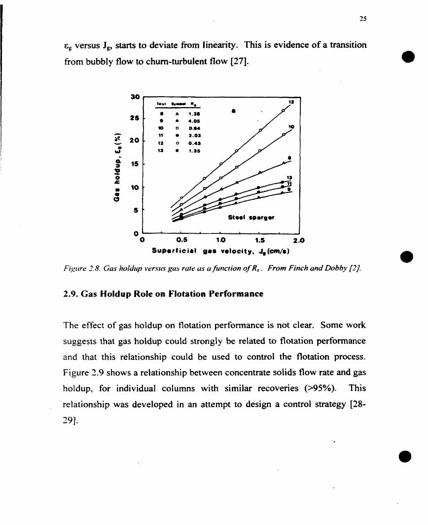
E~ versus J,, starts to deviate fiom linearity. This is evidence of a transition
fiom bubbly flow to churn-turbulent fiow [27]..
30
O O 0.5 1-0 1.5 2 .O
Suparticial 0.8 velocity, J, (cm/*)
Figzlre 3.8. Gas holdicp i7rrsi<s gus rute us u function of R, . Frorn Finch and Dobby [q
2.9. Cas Holdup Role on Flotation Performance
The effect of gas holdup on flotation performance is not clear. Some work
suggests that gas holdup could strongly be related to flotation performance
and that this relationship could be used to control the flotation process.
Figure 2.9 shows a relationship between concentrate solids flow rate and gas
holdup, for individual columns with similar recoveries (>95%). This
relationship was developed in an atternpt to design a control strategy 128-
291.

Little or no correlation between flotation rate constant and the gas holdup
has been reported for mechanical cells. Recent results have however shown
a strong relationship between bubble surface area flux and the flotation rate
constant [ l , 301. Bubble surface area flux is defined by:
From Equation 2.27 we can see that the main dificulty in calculating Sb is
obtaining a reliable estimation of db. This is even more problematic if we
consider that the bubbles have a size distribution rather than a unique size.
Exploring the role of Sb in de-inking flotation columns, Leichtle has
suggested a linear relationship between E, and Sb. Figure 1.10 shows the
results obtained by Leichtle for laboratory and pilot columns [3 11.

Figure 2.10. Cornparison of Sb 10 g using data points j iom all tests (i. e. laboratory and pilot scale columm) [31].
Apart from its possible direct role on flotation performance, gas holdup also
has diagnostic applications. For example, a ruptured sparger is readily
detected as the increase in bubble size will cause the gas holdup to drop
suddenly. . -
2.10. Bubble Surface Area F lux Estimation
The bubble size can be estimatrd by using direct [ l , 30, 321 or indirect
rnethods. Drift flux anûlysis. an indirect method, has been applied to
estimate bubble size in both two phase and three phase systems [2, 33-34].
A brief review of drift flux analysis. taken from Finch and Dobby [2], is
included.

The slip (relative) velocity of gas and liquid in countercurrent systems with
uniform bubbles is defined by :
where upward flow is positive.
The slip velocity is related to the system variables. For bubbie sizes o f
interest here, db =< 2 mm (Re =< 500), a suitable expression is an adaptation
of the multi-species hi~dered settling equation of Masliyah [2 ] , wt-itten
below for the gas-slurry system:
where
and m is a function of the Reynolds number:

1 < Re, < 200
m = 4.45 ~ e 2 . I 200 < Re, < 500
and
where U, is the terminal nse velocity of a single bubble in an infinite pool
(this is calculated using Equation 2.74 and assuming E, = 0).
Using drift flux analysis bubble size can be estimated
E,. Jg and Ji. Following is the step-by-step procedure.
1 ) Set J i = Jr
3 estimate dh;
3 calculate U,, Equation 2.14 with E, =O;
4) calculate Reh. Equation 1-29;
5 ) calculate m. Equation 1.27 or 2.28;
6 ) calculate Reh,, equation 1.19;
7) calculate dh , Equation 1.15; iterate on dh; Go to 2
ffom measurements of

CHAPTER 3: DESIGN CRITERIA FOR GAS HOLDUP SENSOR
3.1 Introduction
- The original sensor designed to measure gas holdup [3-51 experienced a
serious problem in industrial application, with plugging of the syphon ce11
by minera1 particles.
The design of the syphon ce11 had to overcome this problem while respecting
such electrical criteria as cell constant. separation between electrodes, and
electrode width.
3.2 Plugging
The original syphon ceIl was composed of a vertical cylinder (3.8 cm
diameter) closed at its bottom end ( 4 5 O angle) with a lateral opening (about
10 mm diameter) [3]. The first step was to modiQ the bottom of the ce11 to a
conical shape ( I O 0 angle) with an orifice at the bottorn. The second
modification was to increase the ce11 diameter from 3.8 cm to 7.5 cm. With
a larger diameter c d , we are in a position to increase the size of the (sluny

discharge) orifice at the bottom. Giveri that the previous design successfully
prevented bubbles fiom entering at both the top (entrained by the slurry
entenng the cell) and bottom, a sirnilar slurry velocity inside the ce11 can
now be obtained by increasing the orifice diameter. The larger orifice will
reduce plugging by solid particles.
From experience the intemal diameters of both cells were established at 9.6
cm (Do: open) and 7.5 cm (D,: syphon), while the lengths (LT) were
established at 50 cm (in the syphon case, this length includes the conical
section).
3.3 Design Criteria for the Conductivity Cell
In the design of a gas holdup sensor, we have to know the values of the ce11
constants and how they relate to the electrode width and the separation
between electrodes.
Figure 3.1 shows a schematic of the electrode arrangement using both the
open and syphon cells. A thtee-ring electrode arrangement is seen: a cectral
electrode at one polarity, with the two outer electrodes at opposite polarity.
With this design, the current flux is constrained to flow only inside the cell,
allowing for a more stable ceIl constant [4]. In Figure 3.1 W is the electrode
width, D, the intemal ce11 diameter, and L, the separation between
electrodes.
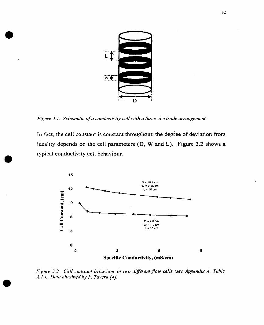
F i g e 3 1 Schemaiic of u condrrcriiiry ceff rith a three-elecrrode arrangement.
In fact, the ce11 constant is constant throughout; the degree of deviation fiom
ideality depends on the ce11 parameten (D, W and L). Figure 3.2 shows a
typical conductivity cell behaviour.
O O 3 6
Specific Conductivity, (&/cm)

23
A simple relationship between the cell parameters and a geometrical ceIl
constant, C, was proposed: Equation 3.1.
where
Using data obtained by F. Tavera during the development of the original gas
holdup sensor (measured ceil constants for di fferent ce11 arrangements) [4],
we can evaluate the effect of the cell parameters on the ce11 constant. From
Figure 3.3 we can see that deviation from th-e geometrical value became less
signiîïcant when the geometricol cell constant decreased. Thus, to ensure
the closest possible estimation of the real ceIl constant, the smallest feasible.
geornetrical value has to be used. C
Another important panrnetcr in thc design of a conductivity ce11 is the
electrode width (W). WC will Jetinc the esposed electrode area by:
.-f,,. = nDCV

Figure 3.3. Deviat ion f iom g~~onrctricul c d consfarrf for 4 cells with 3-elecrrode arrangement. (see =Ippc.nJi\: -4. Tuhie .4.2). Daia O biained by F. Tavera [JI .
Figure 3.4 shows the deviation from geornetrical ce11 constant values
(Equation 3.1 ) for cells with different ratios of AceII/A,v. We can see that the
deviation decreases if the ratio ACcII/A, decreases. As a design criterion a
ratio ACcII/A, equal to I could be chosen. for which W is defined as:
Substituting Equation 3.3 and 3.5 in Equation 3.1 and rearranging terms, we
get that the separation between electrodes necessary to yield a selected ce11 C
constant is given by:

F i 3 Eflect of the rafio ACe,/A,, on deviafion fiom the geomefricai ce11 consfant &y rrsing Equa f ion 3.1 (see Appendk A. Table A. 3). Data obrained &y F. Tavera [4J
3.1. Design criteria for the Syphon Cell
Since the length and diameter of the syphon ce11 are already defined (see
Section 3 4 , the diameter of the orifice, dmifice, at the bottom is the
remaining critical parameter.
Figure 3.5 shows the experimental setup used to characterize different
orifice diameters: 14, 16. 18. 20 and 22 mm. For each diameter, different
water flow rates were passed through the cell until a steady value of H was
obtained.

Fiprc 3 .3 Erperimrntol serup uscd ro churacterize the bottom orifce diurneter of sj phon cell l~&,,/;~$.
A
C . 1
If we apply Bernoulli's pnnciple between point A (ce11 top) and B (ce11
bottom) the water velocity at the top, V,,, is a functinri of H and is given by:
where g is the gravity acceleration. P = 0.5 for laminar flow, and P = 1 for
turbulent flow. The syphon cell diameter is represented by Ds (in this case,
Ds = 7.5 cm). Figure 3.6 shows the experimental data, VA versus H,
obtained for each orifice diameter.
4
9
B
J
H
1
d :13, 16.18, 20 and 22 mm
1 w

Figirrr 3.6. as a funcrion of H for each orajke diorneter, dorflm (See Appendir A. Tables A.4.a and A.4.b).
From section 1.6, when a syphon ce11 is working in a dispersion of slurry
and gas, VA is related to the gas holdup, as follows:
where LT is the syphon ceIl length (in this case 50 cm). Taking equations
3.6 and 3.17 the gas holdup is related to H for a givenVA by:

0 An important parameter to be considered for a particular application, is the
bubble terminal velocity, Ut. A method to estimate this parameter is
presented in Equations 3.8 and 3.9 [2 ] .
where
Figure 3.7 shows the curves V , venus E, (using Equation 3.7), and the
0 bubble terminal velocity, for three different bubble diameters (0.5, 1.0 and
1.5 mm). The bubble terminal velocities were calculated for a water-air
system. For a given application (where E, and db are known), Figure 3.7
indicates that every orifice diameter that gives a V, value lower than U,
(defined by dh) would allow a bubble-free environment inside the cell.
As an example, for a bubble diameter of 1.5 mm, al1 five oritice diameters
could be used (for any E,) because al1 five curves are uiider the terminal
velocity line for a 1.5 mm bubble. If we have a system with E, = 30 % and
db = 0.5 mm, we can use only an orifice smaller than 14 mm.

Figzu-e 3.7. I.:, as a func I ion of G;. -fir rwch or~$ce diameter (LT=50 cm). Bubb1e rerminai \;rlocir ies were esrima~rd us-ing Eqicrrrioris 3.8 artd 3.9 (water-air system. 4 = 1.5. 1. O and 0.5 rnrn)(see Appendik A. IU~/L?.V .-l. 4. tr tmd -4.4. h).
Rearranging Equation 3.6 yields:
where Co and CI are constants u hiçh ;ire independent of the orifice diameter.
Figure 3.8 shows the detemination of Ci, and CI using the data obtained for
the orifices. Substituting these panmeters in Equation 2.17, we can estimate
the maximum orifice diameter as a function of the bubble terminal velocity
and gas holdup (see Figure 3.9).

1200 -- - - . - - ..
Parameters Equation 3.10 Ce = 1.20
Figure 3.8. Determination ofpuron~c.rers Co arrd Cl (Equation 3.10). Data obtained for 5 orifice diamerers (1 4. 16. 18. .?O. und 22 mm).
- - -
4 X I 2 16 20
Bu hbleTcrminal Velocity, cm/s

3.5. Example of Design
A gas holdup sensor was designed for a flotation column application
(mineral system): eg = 10% and db = 1 .O mm. From Section 3.2, Do = 9.6
cm, Ds = 7.5 cm and LT= 5 0 cm (for both cells).
a The two ce11 constants must be the same to use the same conductivity
meter.
O The lowest possible C in this case (LT= 50 cm) is 8 cm.
O Substituting D, and Do in Equation 3.5: W, = 1.9 cm and W, = 1.4 cm.
Substituting C, Ds and Do in Equation 3.6: L, = 7.3 cm and L, = 13.3 cm.
From Figure 3.7. al1 VA values at E, = 10% are lower than U, = 1 1 .I cm/s
(dh = 1.0 mm; water-air system). Considering that smaller bubbles (0.5
m m ) could be present. a orifice diameter, d,nfi,,, of 15 mm is chosen.
Figure 3.10 is a schematic, with al1 dimensions, of the gas holdup sensor
design for this application (E, = 10% and db = 1 .O mm).

Top View Open Cell
Section AB 9.6 cm . -
Syphon Cell
Figr o-e 3.1 O. S c h e s r r i t ic (!/ /lie ,~CJ.V k M / i p pro he J e s i p e ~ l ji>r un applicuiion with .cc 1 0'% (117d dh = 1. O ??l??l.

4.1 Introduction
Two industrial applications in flotation were considered in this work:
mineral concentration (MC0 at Copper Cliff, Ontario) and de-inking of
waste paper (BOWATER at Gatineau, Quebec). The same data acquisition
system is used for both applications: a gas holdup sensor and an electronic
interface that converts the rough signal fiom the sensor to a digital signal,
which can be processed in any cornputer.
This chapter concems the description of the electronic interface, data
acquisition system cal ibration and the two processes. Three gas holdup
sensor units were used. The three sensors have the sarne characteristics as
the ones described in Figure 3 . l 0 (with donecc = 1.5 cm).
1.2. Data Acquisition System.
Figure 4.1 shows a schematic of the electronic associated with the gas
holdup sensor. The sensor (open plus syphon cells) is placed inside the

column. A relay board (Keithley Metrabyte, model REL- 16) perinits each of
the conductivity cells to be measured independently by using a conductivity
meter (Bailey, model TB440). The output of the conductivity meter,
consisting of a signal between O and 10 volts, is converted to digital values
by using an AID converter (Keithley Metrabyte, model DAS-8). The relay
board and the A/D converter are mounted inside a 386.33- cornputer.
b + + Multiplexer
REL-16
1 Conductirneter 1 lllL4
Cornputer 386-33MHz
A A/D Converter " 1 DAS-8
Figirre 4. I . Schematic representation ofthe data acquisition sysrem.
When the digital voltage value (v) is obtained, it is converted to conductance
by using the calibration curve of the conductivity meter (quadratic equation)
relating voltage to conductance, see Equation 4.1.

This conductance value is transformed to conductivity by using the
calibration curve of the specific ce11 that is being read (open or syphon cell).
This ce11 calibration curve is also of the quadratic form. For the open cell,
the equation is as follows:
K,, = An + B,K +C,J2
and for the syphon cell:
K,, = A, + B , K +c,K'
The data acquisition process is driven by a program in Visual Basic 3.0
(Appendix B). Figure 4.2 shows the main menu of the data acquisition
'are.

In order to control the REL-16 and DAS-8 boards, Visual Basic needs
special drivers. To control the REL-16 board and to provide special graph
features the driver package VTX (Keithley Metrabyte) was used. The DAS-
8 board was controlled by using DRIVERLINX-DASSNB (Keithley
Metrabyte).
4.3. INCO: Matte (Cu-Ni) Separation Plant, Column circuit
This plant is located at Copper Cliff, Ontario. The matte separation plant
has five flotation columns (see Appendix C, Figure CA). The main
characteristics of the columns are presented in Table 4.1. Al1 five columns
use Minnovex variable gap jet spargers. Two gas holdup sensors were used
in these tests.
The following experiments were carried out:
a Experiment 1: Sensor 2 \ras placed inside column 2 at a Cmeter depth
for two weeks. The objective \ras to detemine if the syphon ce11 could
work continuousl\. nithout plugginç in an industriai environment.
a Experiment 2 : Sensor I \vas placcd inside column 3 at a 4-meter depth,
and changes in the air f l o ~ rate wcre introduced. Samples of the feed,
concentrate, and tailings. were obtained before and after every air flow
rate change. Grades of Cu. Ni, Co and Fe were determined. Mass
balances were carried out using a method described in the literature [35-
361. The objectives were to determine if the sensor was able to detect
changes in gas holdup. induced by changes of the air -flow rate, and

whether changes in the column performance could be related to gas
holdup.
Table 4.1
Characteristics of lNCO marte separution plant
I i Column I
Height (m) 11.6 11.6 11.6 11.6 Diameter (m) 1.83 1.83 2.13 t -07 Baffles - No Yes / No Y es No S ~ a r g e r TY pe Vanable gap
Air flow (std.m3/hr) 235 - I 233
- - I 340 I 40
<Jas holdup ( O h ) - LU - 25
Midd. Rghr. 1 Lnd L U LIN. 1 Ni C h . 1 Midd. Chu.
Experiment 3: both sensors were placed inside column 3, sensor 1 at a 4-
meter depth and sensor 2 at a 7-meter depth. The objective was to
determine if there were variations in gas holdup with depth.
Calihrdon: Conductivir). meter and Sensor
The conductivity meter calibration was carried out by replacing the gas
holdup sensor with a known resistor, R (R), and reading the voltage value
displayed by the data acquisition software. Using several resistors, a set of
conductance ( 1 / R) values versus voltage was obtained.
The calibration of both cell constants (open and syphon) was carried out by
using electrolyte solutions of known conductivity (without air); the

conductance in each ce11 was measured with the data acquisition software,
using the conductivity meter calibration curve. The conductivity of each
electrolyte solution was measured using a portable conductivity meter
(VWR Scientific, mode1 2052). Calibration parameters for the conductivity
meter, sensor 1 and sensor 2 used in Equations 4.1 to 3, are presented in
Table 4.2.
Table 4.2
Calibrarion parumeters for the conducrivity meter, sensorl und sensor2
(See Appendix C. Tables C. i to C.5)
Conductivity meter Sensor 1 .
Open cell Syphon cell
Sensor 2 Open cell Syphon cell
Parameter
4.4. BOWATER: De-inking Pilot Flotation Column
The equipment was a pilot flotation column constructed of PVC, with an
intemal diameter of 50 cm and a height of 5.1 m. This column is described
elsewhere [3 1,371. The installed instrumentation consisted of mass air flow
meters, magnetic liquid flow meters ( I ) , pressure transducers (3), and
centrifuga1 pumps (2) with control valves (2). The software used for data

collection and control was FIX DMACS (32-bit) by Intellution. The 110
interface between the software and al1 instruments was an OPTOl serial
board by Transduction. The following parameters were continuously
monitored and registered by FIX DMACS: feed and accepts (i.e., underfiow)
superficial flow rates, superfi~cial gas rate, gas holdup obtained fiom pressure
values, bottom pressure, middle pressure, and level.
One gas holdup probe was used in this application: sensor 3. Two kinds of
bubble generating devices were used in these experiments: five sintered
stainiess steel powder (porous rigid) spargers and one variable gap
(Minnovex) sparger.
The experiments carried out were:
O Experiment 1: the E, versus J, was obtained by using the five porous rigid
spargers for three di fferent conditions (Hf= 100 cm; r = 3 min, Hf = 100
cm: r = 6 min, and Ur = 50 cm; t = 6 min). The flotation effkiency and
brightness gain were measured.
Experiment 2: from an initial condition with 5 porous rigid spargen, the
system was evaluated after closing one sparger, and then two spargen.
Two initial conditions were evaluated (J, = 2.5 cm/s; Hf = 100 cm; t = 3
min, and J, = 2.5 cmk; Hf = 100 cm; t = 6 min). The objective was to
detemine the effect on gas holdup and column performance resulting
from a sparger surface area (A,) decrease.

a Experiment 3: fiom an initial condition with 5 porous rigid spargers, the
system was evaluated after closing one sparger, and increasing J, until the
previous gas holdup with five spargers was reached. Two initial
conditions were evaluated (J, = 2.0 crn/s; Hf = 50 cm; T = 6 min, and J, =
1.5 c d s ; Hf = 50 cm; r = 6 min). The objective was to determine if
performance was the same for the same gas holdup obtained in different
ways.
a Experiment 4: the E, versus J, was obtained by using a variable gap
sparger. For this experiment the air flow meter was set to the maximum
(J, = 3.5 cm/s) air flow rate for that gap. The objective of this experiment
was to compare the response o f the system to both sparger types.
O In order to limit errors, al1 the experiments were evaluated 15 minutes after
the steady state was achieved (stable signals). To obtain the flotation
efficiency and brightness gain, pads of feed and accept pulp were prepared
according to the CPPA C.4U method [%]. An average of 10 ERIC values
(ink concentration in the pad) were obtained for flotation efficiency
calculations with an average of 1 O brightness values for brightness gain.
Cnlibration: Conductiviîy meter and Sensor
The calibration procedure of the conductivity meter and the sensor for this
application is the same as the one described in Section 4.3. Calibration
parameters for the conductivity rneter and sensor 3, used in Equation 4.1 to
3, are presented in Table 4.3.

Table 4.3
Calibration parameters for the conductivity meter and sensor 3.
(See Appendix C. Tables C. 6 fo C.8)
1
Conductivity meter Sensor 3
Open cell Syphon cell
Parameters
-7.63239
-0.2756 -0.23 187
4.29777
O. 14052 0. i 2879
0.07425
0.000 15 0.00069

Chapter 5: INCO Results
This chapter describes the results obtained in columns 2 and 3 at the Matte
Separation Plant, INCO limited (Copper Cliff, Ontario). Two gas holdup
sensors were used in these tests. The main objective of these expenments was
to evaluate the re-designed gas holdup sensor under industrial conditions
(especially with regard to plugging of the syphon cell). One o f the sensors
0 was tested continuously for 17 days in column 2. A second test was run in
column 3, to determine if the sensor was able to detect changes in gas holdup
from changes in the air flow rate to the column. Finally, both senson were
installed in column 3. to detemine variations of the gas holdup value with
depth. The raw data are given in Appendix D.
5.1. Test of Reliabiliîy
Figure 5.1 shows the results obtained by gas holdup sensor 2 in column 2 from
March 1 3 to, March 30 ( 1 998 ). Figure 5. l .a shows the gas holdup values and
Figure 5.1 .b, the conductivity values of the dispersion and slurry.

Figwe 5- I . Results on colt~mn 2fiom kfurch 13 to March 30 (sensor 2): (a) gus holdup. (b) conc/irctirity values (dispersion and s lurry). See Appendix D. Tables D. I fo D. 18.

Al1 the values plotted in Figure 5.1 are the averages of fifieen minutes of
a operation. The actual rate of sampling is 1 value per minute. Point A in
Figure 5.1 shows a spike, probably the level in the column was below the
sensor position. The colurnn quickly recovered normal operation, both
conductivity values increasing (unsteady state situation). Between point B
and point C (about 1 day) the column was shut down, both conductivity values
were close to zero since the column was empty. At point C the column was
re-started. Between point C and point D the plant was in unsteady operation.
At point E the air flow was increased (gap between two conductivity values
increases) leading to a gas holdup increase. AAer point E the gas holdup was
stable around 8%, although the conductivity values continued to present
notable changes.
During the test period, the syphon ceIl did not experience any sign of
plugging, even though the column was shut down for almost one day. In the
previous probe design a column shut down caused the syphon to plug. Afier
the test, the sensor was checked with solutions of known conductivity and it
did not show significant deviation from the readings prior to the test, Le., the
calibration (K versus K ) had not changed.
5.2. Response to a- Change of the Air Flow Rate.
Figure 5.2 shows the gas holdup response to a change in the air flow rate
injected into column 3. All the values plotted in Figure 5.2 are the averages of
5 minutes of operation (sampling rate: 1 value per minute). Sensor 1 was
placed at a 4 meter depth.

Figure 5.2. Gas holdup response to changes in the air flow rate to cofumn 3 (31-March- / 998). See Appendix D. Table D. 19
At point A, a change in the superficial air rate was introduced: fiom 1.83 cm/s
to 1.03 crn/s. The gas holdup response was slow, reaching a steady gas
holdup after one hour. In contrast, when the air rate was decreased, fiom 2.03
c m k to 1.69 cm/s (point B), the system quickly reached a new gas holdup.
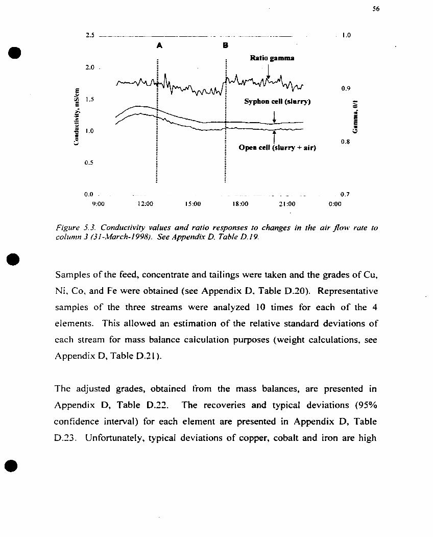
The same data is presented in Figure 5.3, but in terms of conductivity values
and ratio y (dispersion conductivity, open cell, over slurry conductivity,
syphon cell) responses to air flow rate changes. From this figure we can see
that at point B, the dispersion conductivity decreased (increasing the
difference between the two conductivities and giving a higher ratio y).
Ratio gamma I
i Syphon cell (slurry) - k
Figure 5.3. Conduc~iviy values and ratio responses to changes in the air j lo\r . rare ro coltrrnn 3 (3 1 -1March- 1 998). See rlppemiix D. Table D. 1 9.
Samples of the feed, concentrate and tailings were taken and the grades of Cu,
Ni, Co, and Fe were obtained (see Appendix D, Table D.30). Representative
samples of the three streams were analyzed 10 times for each of the 4
elements. This allowed an estimation of the relative standard deviations of
each stream for mass balance calculation purposes (weight calculations, see
Appendix D, Table D.3 1 ).
The adjusted grades, obtained from the mass balances, are presented in
Appendix D, Table D.22 The recoveries and typical deviations (95%
confidence interval) for each element are presented in Appendix D, Table
D.23. Unfortunately, typical deviations of Coppet, cobalt and iron are high

&d conclusions based on these elements are avoided. Fortunately, nickel
typical deviations are low, and can be used.
Figure 5.4 shows the recoveries of copper, nickel, cobalt and iron. Al1 of the
elements exhibit the same trend. Between A and B, we see a slight increase in
the recoveries initially, with a larger decrease at the end. From Figure 5.2, we
know that the gas holdup was increasing duhg this period.
This could be explained by the ohsenations in Figure 5.5. Figure 5.5 shows
the variation in level ( froth depth) during this experiment. From this figure
we can see that the level increased strongly at the end of the period A-B. This
could be related to the recovery decrease.

Figrcre 5.3. Fror h Jeph \*ariations of coltrmn 3 (3 I -March- 1 998). See Appendix D. Table D.24. Dura obtained 6). using a conJltc~irity probe ro d e r e . ~ level.
5.3. Gas Holdup Readings at TWO Different Depths.
Sensor 1 was placed at a 4-meter depth and sensor 2 at a 7-meter depth inside
column 3. Figure 5.6 shows similar results for both sensors. The average gas
holdup of sensor 1. at a +meter dcpth. was 4.7% + 0.1% (95% confidence)
and sensor 1. at a 7-mctcr depth. was 4.9% + 0.1% (95% confidence). These
results show that there was not a significant difference between the two
measurements. This is in contrast with some of the previous work, showing a
gas holdup decrease with increasing depth [ M I .

Figzrre 5.6. Gus holdup signals of sensor I and sensor 2 working at ciifferen! depths inside column 3: sensor 1 ai 4-meter @th: sensor 2 at 7-meter deprh (3-April-1998). See IIppendix D. Tables D.25.a to D.25.c.

CHAPTER 6: BOWATER RESULTS
This chapter describes the results obtained in the pilot column at the De-
inking of Waste Paper Plant, BOWATER Pulp and Paper Inc (Gatineau,
Quebec). Sensor 3 was used in these tests. One objective of the
experiments was to evaluate the re-designed gas holdup sensor on fibre
pulps, which are quite different from mineral slumes. Gas holdup values
obtained from pressure and conductivity were compared. The effect of gas
holdup on flotation efficiency was explored. The relationship between
bubble surface area flux (derived from drift flux analysis) and gas holdup
was tested. Changes in sparger surface area were induced to observe the gas
holdup response and its effect on flotation performance. Finally, a jetting
sparger (MINNOVEX) was tested. The raw data are given in Appendix E.
6.1. Gas Holdup Measurements from Pressure and Conductivity
Figure 6.1. summarizes the results including the ones for the jetting sparger.
From Figure 6.1, some scatter is evident. One explanation is that
conductivity gives a more local estimation than pressure, which is an

average between two points. Differences could be expected if gas holdup
would be distnbuted uniformly in the column
Figure 6.1. Gas holdup BOWATER tests. Every .-lppenJi-r E. Table E. 1.
estimaies fjom conductivity and pressure meusuremenrs for point is the average of 15 minutes of stable operation. See
a
To test it if the difference is signifkant, the t-student value for paired
samples rnust satisfy -1.03 < t (= 1.61) < 3.03, where 2.03 is obtained for
95% confidence and 36 degrees of freedom (t distribution). From this
analysis we c m conclude that the gas holdup obtained from conductivity
( 1 1.47% t 0.44%) is not different from the value given by pressure
( 1 1.77%). A slope analysis (m = 0.87 f 0.02) suggests that the gas holdup
obtained from conductivity, tends to underestirnate the one obtained fiom
pressure at low gas holdup, and to overestimate, at high values.

6.2. Effect of Cas Holdup on Flotation Efficiency
The relationship between flotation efficiency and gas holdup for two
residence times (3 and 6 min) is shown in Figure 6.2. It is clear that gas
holdup affects the flotation eff~ciency, but the latter is also affected by the
residence time, as we expected fiom the discussion in Section 2.7.
Another factor that can affect flotation efficiency is the fioth height. Figure
6.3 shows flotation efficiency venus gas holdup for two fioth heights (50
and 100 cm). For this particular case, Figure 6.3 shows fkoth height does not
seem to strongly affect the flotation performance. One might have expected
a higher recovery in the 50-cm froth case.
r = 6 min
O
T = 3 min
Cas holdup, %
Figwc 6.2. Gus hoidup elflecr on jlortrrion efficiency for IWO reside)tce rimes (3 und 6 r i Froih heighr (Hj is 100 cm. See Appendix E, Tables E. 2 and E. 3.

- - . - . - - - - - -
8 12
Cas holdup, ./.
Figure 6.3. Gas hoidup effecr on j h u r i o n eflciency for hvo fi.ofh heights (50 and 100 cm). r = 3 min- See Appendk E. Tc~hlt~s E.2 u r ~ d E.3.
The effect of sparger surface area. A,. on gas holdup, for two conditions, is
shown in Figure 6.4. When sparger surface area decreases, gas holdup
decreases for the same J,. as seen in Section 2-82. From this figure, we can-
see that the sensor reveals changes in the noise of the gas holdup signal. It
implies that the signal noise is rrlatcd to the bubble size, which increases as
the number of spargen decreasc.~. Thus. the gas holdup sensor could be a
useful diagnostic tool to monitor the spargw.
A test was perfomed to evaluate i F two similar values of gas holdup,
obtained with different sparger surface areas, give similar flotation
efficiency. Figure 6.5 shows the results for two initial conditions.

3 spargers
. - .
Timc
Figtire 6.4. Eflec~ of spurgw srlr$utu orrJtl on prs holdup for mfo conditions: (a) H/ = 100 cm: r = 6 min: 4 = 7 5 ends (hl I I , = i 00 cm r = 3 min: J, = 2.5 cm/s . See Appendix E. Tubles E.3 r~ : , E. 9.

.. - 0 60 . 1.33 cmh k 4 sprrgerr
2.93 cmh 4 spargem
Cas hoidup. O/,
Figure 6.5. Eflecr of sparger surface areo onfloiafion efficiency. Hf = 50 cm; r = 7 min. Ser -4ppendi-Y E. Tables E. 2 and E. 3.
Figure 6.5 indicates that gas holdup alone cannot de fine flotation efficiency.
From this figure we can see that a gas holdup even higher than the initial.
one. produces a lower flotation efficiency. We assume here that the system
chemistry has not changed during the test, which should be verified in future
work.
From Section 1.9, a relationship between gas holdup and flotation
performance could be expected. Figure 6.6 presents flotation efficiency
versus gas holdup for residence times close to 6 min. A relationship is
suggested. A mode1 fit is given with the parameters and a X' statistic
indicated.

FE. =7l.8(1 -~xp(.(&&6)~~)) xz = 3.3 c 16.9 (95% confidence. 9 df)
Gas holdup, %
Figure 6.6. Floiarion eflciencv versus gus holdup for r = 6 min. See Appendix E. Tables E. 3 and E. 3.
A relationship between gas holdup and flotation rate constant has been
reported in mechanical cells for particular cases [ I l . Figure 6.7 shows the
pas holdup versus the collection zone rate constant, k. The collection zone C
rate constant was estimated using the considerations outlined in Section 1.7
(plug flow), assuming Ri equal to 0.5 (same for froth height of 50 and 100
cm). Al1 the results are shown in Appendix E, Table E. 10.
I t is evident from Figure 6.7 that there is some correlation (R' = 0.72)
between the collection zone rate constant and the gas holdup. The scatter in
the data could be explained by changes in the chemistry or rheology of the
feed during the tests.

5 10 15
Cas holdup, ./.
Figure 6.7. Collection zone rate consfant versus gas holdup. Plugflow inside the colurnn M*US asslrmed to calculate rate constant. Froth recovery. RJr is eqtrol50%.. See Appendir E. Tables E. 2 and E- 10.
6.3. Relationship between Sb and E,
To estimate the bubble surface area flux, the bubble diameter was calculated
using drift flux analysis (described in Section 2.10). The properties of the
liquid were assumed to be those of water (psi = 0.01 gkms; psi = 1.0 &cm3)
and bubbles were considered without a load of particles (pb = O gkrn3).
Results giving bubble diameters bigger than 0.2 cm were discarded.
Figure 6.8 shows a linear relationship between gas the holdup and the bubble
surface area flux, as expected from Section 2.9. This relationship shows a
good fit (R' = 0.95).

8 12
Cas holdup, O h
Figure 6.8. Bubble surface area flux versus gus holdup al point is the average of 1.5 minutes of stable operurion. See
323 K and pressure P. Erery Appendix E. Table E. 10.
Following Figure 6.8, if we plot J,/dh (at a pressure and temperature of the
pas holdup measurement) versus gas holdup, we obtain another linear C
relationship (see Figure 6.9). This time however, a slight improvement in
the fit is observed (R' = 0.96). Such a relationship could be used to estirnate
the bubble diameter for a given application.
Bubble surface area flux has been reported having a linear relationship with
the flotation rate constant [ I l . From Figure 6.8 we could anticipate also a
linear relationship between gas holdup and the flotation rate constant. But,
as we saw in Figure 6.7, the gas holdup is not linearly related to the flotation
rate constant.
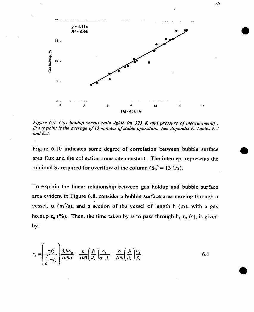
Figure 6.9. Cas hoIdup i*ersirs ruiio Jg/Jh (ut 323 K and pressure of measwement) . Eivery point is the average 4 / 5 rniniifcs 0 f stable operation See Appendix E. Tubles E. 2 un J E. 3.
Figure 6.1 0 indicates some degree of correlation between bubble surface
area flux and the collection zone rate constant. The intercept represents the
minimal Sh required for overflow of the column (Sb0 = 13 US) .
To explain the linear relationship hctween gas holdup and bubble surface
area evident in Figure 6.8. consider a hubble surface area moving through a
vessel, a (m2/s), and a section of thc vcssel of length h (m), with a gas
holdup E, (%). Then. the tirne t<iLcn h?. u to pass through h, (s), is given
by :

O 20 10 60 80 100 120
Bubblc surface area flux, 1 /s
Figure 6.10. Collecrion zone rate constuttt versus bubble surface areayux (ut 273 K and pressure P). Pfugfloar r w s ussunicd to calciriate the rate consfanf. See Appendix E. Tubles E. 2 and E. 1 0.
If we take h = db. then we have a T,," that is independent of db. Rearranging
Equation 6.1 :
The parameter ruo must be a tunciion of the superficial liquid velocity, the
rheology (viscosity and densit~ ot'thc liquid), and bubble load. From Figure
6.8 we can see that the paranleter r.," was independent of JT (the superficial
liquid rate) for these tests. If the system had any significant fluctuation in
rheology, a non-linear relationship between gas holdup and bubble surface
area flux would be expected. In this case, a linear relationship was obtained,
with constant raO. This suggests a constant rheology or may just be an
artifact of taking water as the liquid to estimate bubble size using the drifi
flux analysis. Ta have considered a constant rheology (water) may explain
the absence of a better correlation between the bubble surface area flux and
flotation rate constant.
Substituting Equation 2.1 9 in Equation 6.2 and rearranging:
This relationship is demonstrated in Figure 6.9. Taking the slope of the plot O in Figure 6.8' we have that T, is about I l ms. Therefore, the bubble
diameter c m now be estimated directly from Equation 6.3.

CHAPTER 7: CONCLUSIONS AND FUTURE WORK
7.1 Conclusions
- Some criteria to design the gas holdup probe were established:
The electrode width is a critical parameter in a conductivity
flow ce11 design. An electrode width equal to a quarter of
the cell diameter is recommended.
The lowest possible cell constant is recommended. Cells
with low ce11 constant behave closer to ideality (less
deviation from geometri cal ce1 1 constant).
A simple relationship for three electrode cells was verified,
which relates the geometrical cell constant to the gap
between clectrodes.
A new syphon cell design. having a conical bottom with a
small orifice, was presented.
The syphon ce11 diameter was increased (7.5 cm) from the
original design to allow a larger diameter orifice, which
decreases the chance of plugging.

0 An equation that relates the velocity inside the syphon ce11
(cylindrical part) to the gas holdup and the orifice diameter
was presented. The fluid velocity inside the ce11 must be
lower than the terminal velocity of the rising bubbles to
ensure a fiee-bubble environment inside the syphon cell.
The new design of the gas holdup probe was tested 17 days at INCO Matte
Separation Plant (Copper Cliff, Ontario). The syphon cell did not plug. The
gas holdup probe was able to detect changes in gas holdup upon changes in
air flow rate. Flotation performance (recovery) did not change with air flow
rate, probably due to uncontrolled changes in froth depth.
Tests camied out in waste paper de-inking at BOWATER (Gatineau,
Quebec) showed the gas holdup values obtained by the probe agreed with
those obtained from pressure measurements. This indicates that a bubble-
free environment was obtained inside the syphon cell.
Tests carried out using sparger surface areas showed that the noise
associated to the gas holdup signal could be related to the bubble diameter.
This noise may be used to diagnose sparger operation.
Gas holdup is an important variable in flotation, but alone does not define
flotation performance. The relationship between the gas holdup and the
collection zone rate constant showed some degree of correlation. Chernistry
and rheology of the feed are other factors to be considered. Bubble surface
area flux also showed little correlation with the collection zone rate constant.

The dispersion in the Sb data might be related to the assumption made to
calculate the bubble diameter using the drift flux analysis.
From a conceptual analysis, the bubble surface area flux would be a function
of the gas holdup and a parameter raO. This parameter is defined as the time
it takes a bubble surface area, moving through a vessel, to cover a distance
equal to the bubble diameter. This parameter seems to be constant for a
system with constant rheology. A Iinear relationship between gas holdup
and bubble surface area flux is predicted. This linear relationship was
verified in Chapter 6.
7.2 Future Work
The potential use of this sensor in the diagnostic of sparger operation may
justify further exploratory research in that direction. Trying to relate
changes in the noise of the gas holdup signal to changes in bubble diameter
is one approach.
An exhaustive analysis of the gas holdup relation to the bubble surface area
f l ~ i s is recommended. Minerd systems may have smaller changes in
rlicolorrv L d than those we suspect occurred For waste paper de-inking.
Gorain, B.K., "The Effect of Bubble Surface Area Flux on the Kinetics of
Flotation and its Relevance to Scale-Up". Ph.D. Thesis, University of
Queensland, Australia, 1997, pp. 59-1 44.
Finch, J.A. and Dobby, G.S., Column Flotation, Pergamon Press, 1990.
Gomez, CO., Tavera, F., Finch, J.A., Perez, R. and del Villar, R., 1995
(b). "Continuous Gas Holdup Measurements in Flotation Columns".
Proc. IV Meeting of the Southem Hemisphere on Mineral technology,
Castro S. and Alvarez J. Editors. Vol. 3, Concepcion, Chile, 1994; pp.
123- 136.
Tavera, F., "Flow Cells to Measurr Electrical Conductivity: Use in
Estimating Gas Holdup in Flotation Systems". Ph.D. Thesis, McGill
University. Canada. 1996.
Tavera. F., Gomez. C O . and Finch. LA.. "Novel Cas Holdup Probe and
Application in Flotation C'olut~ins". 'I'rans. Instn. Min: Metall. (Sect. C:
Mineral Process. Esir. MetriIl. ). 105. May-August 1996, pp. 99- 104.
Condon, E.U. (Ed.). Handbook of Physics. Chapter 9, McGraw Hill Book
CO., 1 967, pp. 146- i 69.
Andrews, D.H., I ntroductory Physical Chemistry, McGraw Hill Book
Co., 1970, pp. 689.

8. Barrow, G.M., Physical Chernistry, McGraw Hill Book Co., 1973, pp.
787.
9. Adamson, A.W., A Textbook of Physical Chemistry, Academic Press,
1979, pp. 953.
1 O.Kasper, C., "The Theory of the Potential and Technical Practice of
Electrodeposition", Trans. Electrochem. Soc., 1940, Vol. 77 pp. 353-384,
Vol. 78 pp. 131-161.
1 1 .Atkins, P. W., Physical Chemistry, W.H. Freeman and Company, 1981,
pp. 1095.
P.Levine, LN.. Physical Chemistry, McGraw Hi11 Book Co., 1988, pp. 920.
13.Braunstein. J. and Robbins, G.D., "Electrical Conductance Measurements
and Capacitive Balance". J. Chem. Ed.. 197 1, Vol. 48, No. 1, pp. 53-59.
14.Gilmont. R.. and Walton, R. F.. "New Design of an Electrolytic Ce11 for
the Study of Electroplating Phenomena", Jour. Electrochem. Soc., 1956,
Vol. 103, No. 1 O, pp. 549-552.
I5.Lord Rayleigh, "On the Influence of Obstacles Arranged in Rectangular
Order Upon the Propenies of a Medium", Phil. Mag., 1892, Vol. 34, pp.
48 1-502.

lG.Meredith, R.E and Tobias, C.W., "Resistance to Potential Flow through a .
Cubical Array of Spheres", J. Appl. Phys., 1960, Vol. 3 1, No. 7, pp.
17.Wagner, C., "The Scope of Electrochemical Engineering", in Advances
in Electrochernistry and Electrochemical engineering, Vol. 3. (ed.
Tobias, C. W.), Inerscience Publishers, 1962, pp. 1 - 14.
18.Shen, G., "Bubble Swarm Velocities in a Flotation Column". Ph.D.
Thesis, McGill University, Canada, 1 994.
19.Maxwel1, J-C., A Treatise of Electricity and magnetism, 3rd Edn., Oxford
university Press, 1 891. Vol. 1. part II, Chapter IX, pp. 435-449.
20.Tumer. J .C .R.. "Two-Phase Conductivi ty-The Electrical Conductance of
Liquid Fiuidized Beds of Spheres". Chem. Eng. Sci., 1976, Vol. 3 1 , pp.
487-492.
2 I .Y ianatos. J.B.. "Column Flotriti.on Froths", Ph.D. Thesis, McGill
University. Canada. 1987.
1 2 . X ~ . M.. "Radial Gûs Holdup Protilr and Mixing in the Collection Zone
of Flotation Columns". Ph.D. Thesis, McGill University, Canada, 1990.
23.Uribe-Salas, A., "Process Measurements in Flotation Columns Using
Electrical Conductivity". Ph.D. Thesis, McGill University, Canada, 1991.

24. Wills, B.A., Mineral Processing Technology, Pergamon Press, 1993.
25.Banisi, S., Finch, J.A., Laplante, A.R. and Weber, M.E., "Effect of Solid
Particles on Gas Holdup in Flotation Columns - 1. Measurements",
Chem. Eng. Sci., 1995, Vol. 50, No. 14, pp. 3319-2334.
26.Banisi, S., Finch, LA., Laplante, A.R. and Weber, M.E., "Effect of Solid
Particles on Gas Holdup in Flotation Columns - II. Investigation of
Mechanism of Gas Holdup Reduction in Presence of Solids", Chem. Eng.
Sci., 1995, Vol. 50, No. 14. pp. 335-2342.
27.Xu. M. and Finch. J.A.. "Eflrct of Sparger Type and Surface Area on
Bubble Size in a Flotation colurnn". Canadian Metallurgical Quarterly,
1989. Vol. 38 ( 1 ). pp. 1-6.
XDobby. G.S.. Amelunscn. K. and Finch. J.A., "Column Flotation: some
Plant Esperience and h l d c l I>cvelopment", Symp.. Automation for
Mineral Resourcc Dwcl.. .-Iiisir<iliri. 1985. pp. 559-264.
29.Arnelunsen. R.. "'Hi2 !tlcch.irii~-3 <if Opention of Column Flotation
Machines". Proc. 17"' :\nnci.il Mxt ing of the Canadian Mineral
Processors. C.1 .M.. Jmucir? I W 5 . pp. 1 - 7 4 1 .
30.Gorain, B.K., Manlapig. E X . and Fnnzidis, J.P., "The Effect of Gas
Dispersion Propefiies o n ihc Kinctics of Flotation", Proc. of the
international Symposium on C'olumn Flotation (Gomez. C.O. and Finch,

J.A. ed.), the Metallurgical Society of the Canadian Institute of Mining,
Metallurgy and Petroleum, Montreal, Canada, 1996, pp. 299-3 1 3.
3 1 .Leichtle, G.F., "Analysis of Bubble Generating Devices in a De-inking
Column", Master Thesis, McGill University, Canada, 1998.
3?.Yianatos, J.B. and Puelle, P.C., "Development and Calibration of a
Flotation Bubble Size Sensor", Proc. IV Meeting of the Southem
Hemisphere on Mineral technology, Castro S. and Alvarez J. Editors.
Vol. 4, Concepcion, Chile. 1 994, pp. 1 57- 164.
33. Wallis, G.B., One Dimensional Two-Phase Flow, McGraw Hill Book
Co., 1969, Chapter 9.
34.Banisi. S. and Finch. J A . . Tcchnicd Note: " Reconciliation of Bubble
Size Estimation blethods Using Drift Flux Analysis", Minerals Eng.,
1997. Vol. 1 O. p l i 367-380.
35. Simpson. D E . \'ol lcr. \'.K. and i%rrcti. M.G.. "An Efficient Algorithm
for Minera1 Procrssin< d;)t;i Adjiistriicnt". Int. J. Miner. Process., 199 1 ,
NO. 3 1 , pp. 73-96
36.Cortés-Lopez. F.. "liwluriç iim del Comportamiento de la Molibdenita en
el Circuito de Flotacion C'olcctiva de Division Andina de CODELCO-
Chile", B.Sc. Thesis. Uniwrsidrid Técnica Fedérico Santa Maria, Chile,
1994.

3 7. Watson, J.A., "De-inking Recycled Paper Using Co lumn Flotation".
Master Thesis, McGill university, 1996.
38.CPPA Usefbl Method C.4U, "Forming Pads for Reflectance Tests of
Pulp", CPPA Usefbl method, CPPA Standard Method.

APPENDIX A
Table A. 1. Conduciivity and conductame values obtained for nt.0 3-elecrrode c e f k Data obtained by Francisco Taveru [4]

Tub le A. 3. Cell constants (measured and geometrical) for three electrode width (3- electrode cells). D = 7.5 cm: L = 10 cm. Data obtained by Francisco Tmera [-/]
Tubir .J.-l.u. Liqrrid relocify inside the syphon cell as function of gus holdup and H (as
18 mm H Eg VA
(cm) ( O ) (cm/s)
3.6 7.2 4-20 4.0 8.0 4.47 6.1 12.4 5.67 6.7 13.4 5.94 8.7 17.4 6.70 8.9 17.8 6.82
I 1.8 23.6 7.96 12.2 24.4 8.1 1 14-5 29.0 8.85 15.1 30.2 9.10 17.3 34.6 9.75 18.1 36.2 10.00
. 14 mm
H
(cm) 7 6 -. 4.1 5.6 7.4
1 1 . 1 1 1 . 1 15.5 19.9
4 ( O h )
3 2 8.2
I 1.2 14.8 22.2 22.2 3 1.0 39.8
V A (cm/s)
7 70 - .- 2.87 3.30 3-84 4.71 4.75 5.59 6.30

Table A. 4. b. ContinuarionJion Table A. 4. a.
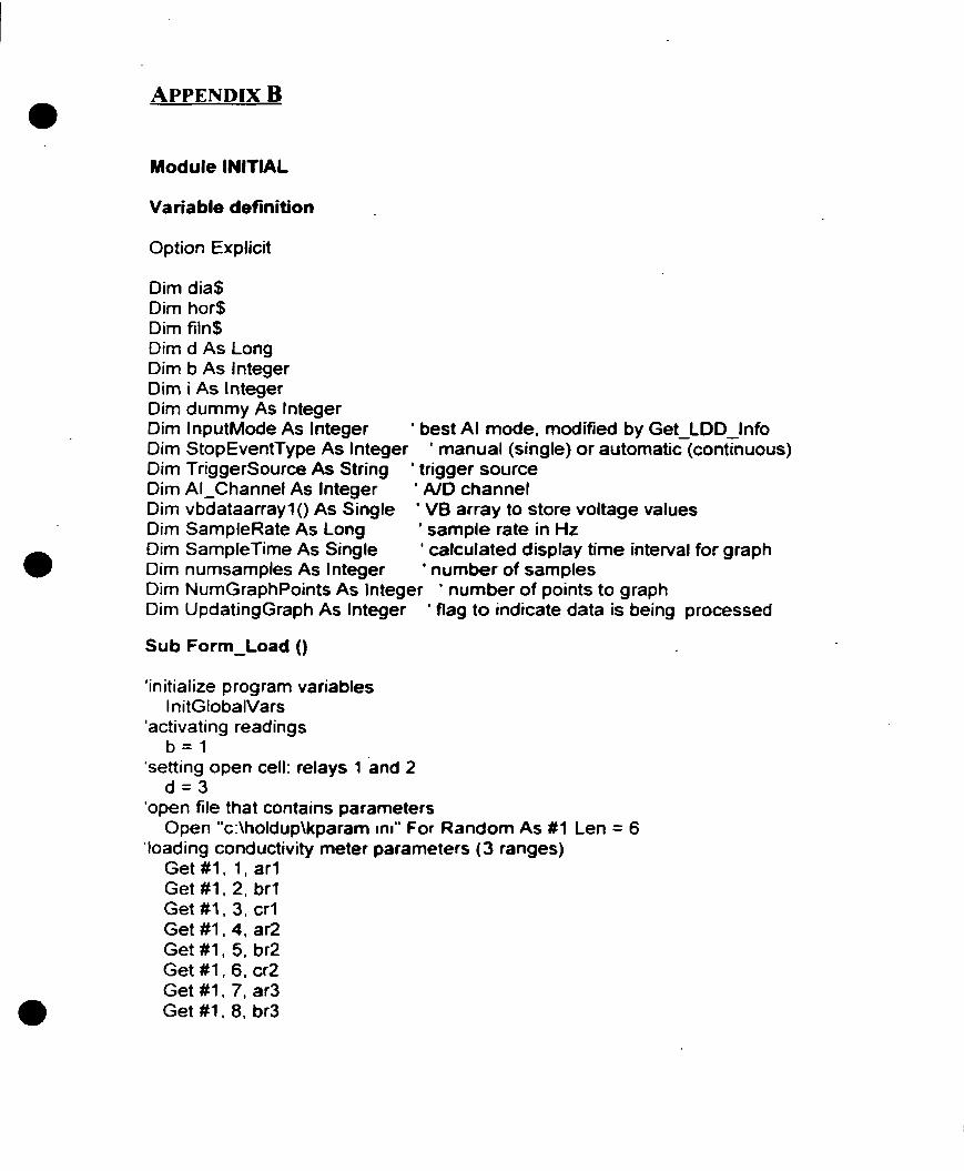
Module INITIAL
Variable definition
Option Explicit
Dirn dia$ Dirn hor$ Dirn fiIn$ Dim d As Long Dirn b As lnteger Dirn i As lnteger Dirn dummy As lnteger Dirn InputMode As lnteger ' best Al mode, moâified by Get-LOD-lnfo Dirn StopEventType As lnteger ' manual (single) or automatic (continuous) Dirn TriggerSource As String ' trigger source Dirn AI-Channel As lnteger ' AID channel Dirn vbdataarrayl () As Single ' VB array to store voltage values Dim SampleRate As Long ' sample rate in Hz
a Dirn SampleTime As Single ' calculated display time interval for graph Dirn numsamples As lnteger ' number of sarnples Dirn NumGraphPoints As lnteger ' number of points to graph Dim UpdatingGraph As lnteger ' flag to indicate data is being processed
Sub Form-Load ()
'in itialize program variables InitGlobalVars
'activating readings b = l
'setting open cell: relays 1 and 2 d = 3
'open file that contains parameters Open "c:\holdup\kparam mi" For Random As 81 Len = 6
'loading conductivity meter parameters (3 ranges) Get #1, 1, ar l Get #1, 2, br l Get #1, 3, cr l Get #1, 4, ar2 Get #1, 5, br2 Get #1, 6, cr2 Get # I l 7, ar3 Get #1, 8, br3

Get #1, 9, cr3 'defining active conductivity meter range
Get #1, 22, r 'loading open cell parameters
Get # I l 10, a01 Get #1, 11, bo l Get #1, 12, col
'loading syphon ceII parameters Get #1, 13, as1 Get #1, 14, bs1 Get #Il 15, csl Close #1
'setting relays related to the conductivity meter I f r = l T h e n a = O If r = 2 Then a = 40960 If r = 3 Then a = 61440
'setting control status editexesrEnabled = False 'start disable command2.Enabted = False 'sensor disable comrnand3.Enabled = False 'conductivity meter disable command5.Enabled = False 'end disable cornmandl .Enabled = True 'stop enable
'setting date and time dia$ = Date$ hors = Tirne$
'defining name of data file fiIn$ = "c:\data\" + MidS(dia$. 9. 2) + Left$(dia$, 2) + Mid$(dia$, 4, 2) + ".datWt
'displaying date and time on INITIAL from fecha.Caption = dias hora-Caption = Times
'closing relays rel-DOScalar = d + a rel.ArmState = 1 'running relay control
End Sub
Sub InitGlobalVars ()
'initialize variables 'Al-Channel = O 'SampleRate = 10000 'numsamples = 1500 StopEventType = DL-TCEVENT
End Sub

Sub reiJrocessDone (WamingCode As lnteger)
a . 'routine associated to relay control
reLArmState = 2 Call waiting(8) das8
End Sub
'stopping relay control 'calfing delay routine 'calling AIC converter routine
Sub waiting (s As Integer) 'delay routine
Dirn ax As lnteger Dim m$ Dirn tnew$ Dirn tne - Dirn told
ax = O told = O
30 ttt$ = Tirne$ tnew$ = Mid$(ttt$, 8, 1) tne = Asc(tnew$) If told = O Then told = tne If tne = told GoTo 30 ax = ax + 1 told = tne If ax < s GoTo 30
End Sub
Sub das8 () ' N C converter routine
ReDim vbdataarrayl(1500) Dim j As lnteger Dirn in As lnteger 'defining number of samples and sampling rate (Hz)
numsamples = 1500 SampleRate = 10000
'initiaking N C converter board init-device sr-ai
'defining A/C converter parameters sr-ai. Reqop = dldevice sr-ai.Req-device = O sr-ai. Req-subsystem = d l a i soi.Req-mode = dljolled
'starting AIC converter

sr-ai.Req-0~ = dl-start sr-ai. Refresh
' Call procedure ta start data acquisition GetAnalogBuffer sr-ai, InputMode, AI-Channel. numsamples. SampleRate. StopEventType 'Filling the output array
durnmy = VBArrayBufferConvert(sr-ai, O, 0. numsamples, vbdataarrayl (O), DL-tsingle, O, 0)
End Sub
Sub SR-AI-ServiceDone (task As Integer, device As Integer, subsystem As Integer, mode As Integer) 'routine associated to N C converter control
If (d = 3) Then 'identifying cell 'calculating the average voltage measured for the open cell
aux = O For i = 1 To 1500
aux = aux + vbdataarrayl (i) Next i vo = aux / 1500
'calculating open cell conductance aux = conductance(r, vo) vol = VO
'calculating open cell conductivity ko = a01 + bol ' aux + col ' aux * aux
'displaying open cell conductivity advafuel .Text = Format(Str$(ko), "#.##") advaluel Refresh advaluel .ArrnState = 1 'running open cell label control
Else 'calculating the average voltage measured for the syphon cell
aux = O - For i = 1 To 1500
aux = aux + vbdataarrayl(1) Next i vs = aux 1 1500
'calculating syphon cell conductance aux = conductance(r, vs) vs1 = VS
'calculating open ceIl conductivity ks = as1 + bs1 ' aux + csl ' aux ' aux
'dispiaying open cell conductivity

advalue2.Text = ~orrnat(Str$(ks); "#-WB) advalue2 .Refresh advalue2.ArmState = 1 'ninning syphon cell label control
End If
End Sub
Function conductance (r As Integer, aux As Single) As Single
If r = 1 Then conductance = arl + b r l ' aux + c r l ' aux 'aux If r = 2 Then conductance = ar2 + br2 " aux + cr2 ' aux ' aux If r = 3 Then conductance = ar3 + br3 * aux + cr3 *aux ' aux
End Function
Sub ADVALUEI-ProcessDone (WarningCode As Integer) 'routine associated to open cell label control
advaluel .ArmState = 2 d = 12 relay (a + d)
End Sub
Sub relay (m As Long) 'relay routine
closing relays forml .rel.DOScalar = m form 1 .reI.Refresh forml .rel.ArmState = 1
End Sub
'stopping label control ' setting syphon cell: relays 3 and 4 ' calling relay routine
'setting relays
'running relay control
Sub ADVALUE2-ProcessDone (WarningCode As Integer) 'routine associated to syphon cell label controt
advalue2.ArmState = 2 d = 3 graph 1 .ArmState = 1
'stopping label control 'setting open cell relays: 1 and 2 'running conductivity graph control
End Sub
Sub GraphlProcessDone (WarningCode As Integer) 'routine associated to conductivity graph control
Dim aux1 As Currency Dim aux2n As Single

Dim aux3n As Single graphl .Anstate = 2 'stopping conductivity graph control aux2n = Val(advalue1 .Text) If aux2n < .O1 Then aux2n = -001 aux3n = Val(advalue2.Text) If aux3n < -01 Then aux3n = -001
'calculating ratio y auxl = (aux2n) / (aux3n)
'calculating gas holdup aux1 = (1 - auxl) / (1 + -5 ' auxl) eg = auxl ' 100 holdup.Text = Str$(eg) holdup.Refresh holdup.AmState = 1
'displaying gas holdup value
'ninning gas holdup label control
End Sub
Sub holdup-ProcessDone (WarningCode As Integer) 'routine associated to gas holdup label control
holdup-ArrnState = 2 'stopping gas holdup label control GRAPH2.ArmState = 1 'running gas holdup graph control
End Sub
Sub graph2-ProcessDone (WarningCode As Integer) 'routine associated to gas holdup graph control
GRAPH2.ArmState = 2 'stopping gas holdup graph control 'open file to save data
Open fiIn$ For Append As #l Print #1. hor$, Format(vo1, "#.#Mt"). Format(vs1, "#.fi##'') Close #1
'determining if click on stop If b = O Then
'stopping data acquisition b = l d = 3 'setting open cell: relays 1 and 2 editexesr. Enabled = True 'start enable cornmand2.Enabled = True 'sensor enable command3.Enabled = True 'conductivity meter enable command5.Enabled = True 'end enable editexesr.SetFocus GoTo 100 'stop data acquisition
End If Start 'calling routine start

100 End Sub
Sub start () 'routine start
'defining date and time .
hor$ = Tirne$ dia$ = Date$
'defininig name of data file fiIn$ = "c:\data\" + Mid$(dia$. 9. 2) + Left%(dia$. 2) + Mid$(dia$, 4. 2) +
".datu 'displaying data and time
fecha-Caption = dia$ hora.Caption = Time$ relay (a + d) 'calling relay routine
End Sub
'if a control (button) is enable can induce an event (click)
Sub Commandl-Click () 'routine executed after click on stop button .
b = O command 1 .Enabled = False 'stop button disable
End Sub
Sub Command2-Click () 'routine executed after click on conductivity meter button
form 1 .Enableci = Faise form3.Show
End Sub
Sub Command3-Click () 'routine executed after click on sensor button
form 1. Enabled = False form2.Show
'initial form disable 'Go to conductivity rneter module
'initial form disable 'Go to sensor module
End Sub

Sub editexesr-click () 'routine executeâ after click on start button
editexesr. Enab ted = False comrnand2.Enabled = False cornmand3.Enabled = False command5Enabled = False commandl .Enabled = True commandl .Setfocus start
End Sub
Sub CornmandS-Click () 'routine executed after click on end button
End
End Sub
'start button disable 'sensor disable 'conductivity meter disable 'end button disable 'stop button enable
'calling start mutine
'end of program
Module General 'Copyright 1994 DriverLlNXNB Source Code Example Library
Option Explicit
Dim i As fnteger Dim dummy As lnteget Global aux As Single Dim Sample() As Single Dim NumSamples As Integer Dim numchannels As lnteger
Conductivity meter parameters Global r As lnteger
Range 0.1 Global arl As Single Global br1 As Single Global crl As Single
' Range 1 .O Global ar2 As Single Global br2 As Single Global cr2 As Single
' Range 10 Global ar3 As Single Global br3 As Single

Global cr3 As Single
' Siphon cell parameters Global as1 As Single Global bs1 As Single Global cs1 As Single
' Open cell parameters Global a01 As Single Global bol As Single Global w l As Single
Global ko As Single Global ks As Single Global eg As Single Global vo As Single Global vs As Single
Global a As Long
Global vol As Single Global vsl As Single
Sub GetAnalogBuffer (SR As Control. Mode As Integer. Channel As Integer. NumSamples As Integer. SampleRate As Long. StopEventType As Integer)
' Specify timing event SR.Evt_Tim-type = DLRATEEVENT SR.Evt-Tim-rateChannel = DCDEFAULlTIMER SR-Evt-Tim-rateMode = DL-RATEGEN SR. Evt-Tim-rateclock = DL-INTERNALA
'lkample rate in Hz SR. Evt-TimratePeriod = DLSecsZTics(SR. SR-Evt-Tim-ratechannet (1 1
SampleRate))
' Specify start event SR.Evt-Str-type = DL-COMMAND
SR-Evt-Str-type = DL-AIEVENT ' SR-Evt-Str-aiChannel = O ' SR-E-Str-aiGainCode = DLGainPCode(SR. -1) ' SR-Evt-Str-aiUpperThreshold = 1000 ' SR.Evt-Str-aiLowerThreshold = 900 ' SR-Evt-Str-aiSIope = True
' Specify stop event SR. Evt-Stp-type = StopEventType

' Specify number and size of buffers SR.Sel-buf_N = 1 SR-Sel-b-ize = DLSamplesZBytes(SR. Channel. NumSamples) SR-Sel-buf-notrfy = True
' Specify data format and channels to acquire SR-Sel-chan-format = DLtNATlVE SR-Sel-chan_N = 2 SR-Selchan-start = O SR-Selchan-startGainCode = DLGain2Code(SR, 1 ) ' unipolar, unity gain SR-Selchan-stop = Channel SR-Selchan-stopGainCode = DLGain2Code(SR, 1) ' unipolar, unity gain
' Initiate the Service Request SRSR-execute = 1
' Display a result message End Sub
Sub init-device (SR As Control)
'initialize device and service request control SR.Req-subsystem = DL-device SR.Req-mode = DL-other SR.Req-op = DL-INITIALIZE
End Sub

BESSEMER MA-€

Table C. 1. Calibration data. conduct ivity meter for M O tests. .
8 Average ' 068 -- 2.069 2.815 2.817 3.575 3.573 4.304 4.299 5.022 5.016 5.707 5.701 6.420 6.410 7.181 7.169 7.838 7.823 8.420 8.a3 8.918 8.897
Tuhle C. 2. Calibra fion data. open ceif qf sensor l for I'VCO tests.
S 10 . -
6.05 7.40 9.55 12.49 15.16 17.93 21.12 23 -85
Average 4.20 6.05 7.39 9.55 1 2.18 15.16 17.93 21-12 23.83

Table C.4. Ca/ibralion data. open ce// of sensor 2 for iNCO tests.
Average
0.62 0.80 1 .O8 1.18 1'86 2.26 2.74 3.12
TXdr C. S. Calibra~ion duru. s~pllon cdl of sensor 2 for INCO rem.
Average
0.62 0.80 1 .O8 1.48 1.86 2.26 2.71 3.1 t
Average
2.797 3.631 4.445 S. 236 5.998 6.789 7.639 8.36 1 8.999 9.490

Table C. 7. Calibrafion duru, open cetifor BOWATER tests.
Average 6.24 10.63 14-19 18.87 24.10 29.25 34.26 39.3 I
Tubk C. 8. Calibrurion duru. s~pitort ce// for BOIK4 TER resrs

APPENDIX D
Table D. 1. INCO Matfe Separafion Plant column 2. Gus holdup dura collected hfarch

99
Table D.2. INCO LMarte Separaiion Plant column 2. Gas holdup data collected i e c h
Lg (Y* ) 8.48
8.47 8.63 8: 50 8.19 8.25 8.52 8.48 8.36 7.9 1 8.27 7.75 7.62 7.02 7.50 7.79 7.83 7.40 7.57 7.x5 7.57 7.47 7 2.3 - - 7: ' 43 7 10 7 52 7 X? O - ' . 5 - o. , -8
?hl - -0 - -n - M i
- 1: - -- - t.1 - - 7
+
- t,G - C'
- 'JI t X? - 54 - -* 1 1 -
7 71 7
'hl 7 3
k sypnon (mS/cm)
7 - - 1.01 1-01 1 .O0 1 .O0 0.99 0.99 0.99 0.99 1.00 1.00 1.01 1 .O2 1 *O2 1 .O2 1 .O3 1 .O3 1 .O3 1-03 1 .O3
. 1 .O3 1 .O1 1.06 1-07 1 .O9 1-10 1.1 I 1.11 1.13 1.13 1.13 1.13 1.12 1.1 I 1.10 I .O4 1 .O8 1 .O7 1 .O7 1-06 I -0s 1 .O5 I .O4 1.03 1 .O2 1-01

Table 0.3. INCO Mutte Separation Plant c h m n 2. Gus holdup data col/ected March 15 (1 998) using sensor 2.
w open (mSfcm) 0.89
0.89 0.88 0.88 0.88 0.87 0.87 0.88 0.88 0.87 0.87 0.87 0.88 0.87 0.87 0.87 0.87 0.86 0.86 0.85 0.86 0.86 0.85 0.84 0.84 0.82 0.82 0.8 1 0.82 0.82 0.8 1 0.8 1 0.80
0.8 1 0.8 1 0.n 1 0.82 0.83 0.83 0.85 0.88 0.9 1 0.93 0.94 0.95 0.96 0.95 0.95 0.93
w sypnon 1 (mSkm) 1.01 1 .O0 0.98 0.97 0.97 0.96 0.95 0.94 0.93 0.93 0.93 0.93 0.93 0.91 0.95 0.96 0.99 1 .O I 1-03 1 .O6 1 .O8 1-10 1.11 1.12 1.12 1.1 1 1.10 1-10 1.09 1 .O8 I .O8 1 .O7 1.06 1 .O6 1 .O5 1 .O5 1 .O3 1-04 I .O4 1 .O3 1 .O2 1-02 1 .O2 1 .O2 1 .O2 1 .O2
r open (mS/cm)
0.9 3 0.9 1 0.90 0.89 0.88 0.87 0.87 0.8 1 0.8 I o. 80 0.80 0.79 0.8 1 0.8 1 0.82 0.83 0.86 O. 89 0.9 1 0.93 0.95 0.96 0.98 0.97 0.97 0.97 0.97 0.96 0.95 0.96 0.96 0.96 0.95 0.95 0.94 0.94 0.93 0.93 0.93 0.92 0.9 1 0.9 1 0.9 1 0.91 .
0.9 1 0.9 1
m

101
Table D.4. INCO Matte Separorion Plant column 2. Gus holdup data collecred March

101
Table D.5. INCO Matte Separation Plant colzrmn 2. Gas holdrrp data collecred Jhrcli
K sypnon (mS1cm) 7 m r
0.928 6.93 0.93 0.93 0.93 0.93 0.93 0.93 0.93 0.93 0.94 0.95 0.95 0.96 0.96 0.97 0.97 0.07 0.w O 97 o 97 11 YX
0 9%
0 crX O crn t 1 ' J X
O &JX
( t ' f i #
(1 V'I
O '4')
(1 ' F b
(1 'F4
1 tr l
[ i i !
l i a i
1 i n i
1 l m 1
I l ' C d
I I ' F I
t l '4s (1 ' 4 X
O un ( 1 (J-
( 1 '4s 0 ' 4X
( 1 '1-
Il 'lx ( I vx -
k sypnon (mS/cm)
0-99
1 .O0 1 .O1 1 .O2 1 .O2
-1 .O3 1 . 0 1 1 .O6 1.1 1 1-15 1.18 1.17 1-15 1. Id 1.13 1.12 1.12 1.12 1.12 1.13 1.13 1.13 1.13 1.14 1-15 1.17 1.18 1.20 1.21 1.22 1 . 3 1 -24 1 -24 1.25 I . 3 1.25 1.25 1-24 1.24 I .Z3 1.12 i 22 1.21 1-21 1.21 1-20

Table D.6. INCO Matte Separafion Plant column 2. Gus holdup data collected March 18 (1 998) using sensor 2.
#
0:22:40 0:37:42 0:52:46 1:07:49 1 :22:5 1 1 :37:57 1 :53:O2 2:08:06 2:X :O9 X 8 : 14 2:53: 17 3:08: 18 3 2 3 2 1 3:38:23 3 5 3 2 6 J:08:27 4 2 3 2 9 4:38:3 1 1:53:36 5:08:38 5:23:J 1 5:38:46 5 5 3 3 1 6:OX:F-l 6:23:57 h:39:00 6:SJ:02 7:09:02 7:24:07 7:;v: IO ?;M: 14 n.00. 1 t i X:2J:2 1 X:30:2j X:Sl.I4 '#:09:27 Y:24.2V 9: 39: j 5 9:5J:40 l OWi: J2 I0:2J:J7 1 O: j9: J9 10:jJ:jO 1 1 :09:53 1 1 :24:55 l 1:40:0l 1 I :55:04 12: IO: (KJ
k ' ' P B (mSlcm)
1.0/ 1 .O7 1 .O4 1.06 1 .O6 1 .O4 1 .Cu 1-04 1 .O3 1 .O3 l .O3 1-02 1 .O3 1 .O3 1.02 1-01 1 .O1 1.01 1 .OC)
1 .O()
1 .(Ml
I .OZ I .O I 1 .O2 1.02 1 .O'
1 .O3 1 .O<
1 0' 1 ( 1 1
1 H l
I (il ( t <FI
O 'W
O 'U,
O 9 5 0 ')J
i t (1;
O 'II
( 1 '):
i t ' ) Z 0 OZ
0.9;
0 . 0 5
0.95 0.95 O.'H* o. oh (i.9..
E7YJjm (mS/cm) l m r
1.190 1.19 1.18 1.18 1.17 1.17 1.16 1.15 1.15 1.14 1-14 1.1 J
1.14 1.11 1-13 1.13 1.12 1.12 1.12 1.12 1.13 I . I J I.1J 1 I J I 1' 1. 15 1.15 1 I J I 1; 1.1:
1 II I I i J f 1 in. I if(
I IJ 1 1,:
I il'
1 Il' I il: 1 o; 1 o'i 1 OP
1 0 5 l tut
1 (n, 1 in1 1 tu?

104
Table 0 . 7 . INCO Matte Sepuration Plant column 2. Gas holdup data collected :tfurch
I Z:J5:ZJ l3:ûO:X 13: 1 S:32 13:30:33 13:45:34 1 J:00:37 14: I5:38 l4:3O:39 14:45:13 1 5:00:46 15:15:51 15:30:54 15:45:59 l6:ûû:J9 16: 1559 l6:3 1 :O2 l6:-t6:O7 17:01:13 17:16:15 17:31:17 17:46:7 1 18:C) 122 ln: 1623 183 125 18:46:30 l9:O 1 5 6 19: 16:39 19:; 1:40 1 9:46:45 2o:o 1 145 20: lh:J7 2o:j 1:49 31~4Ci:Sj 2 l :O 155 ZI:17:01 2 I :32:06 21:47:[ 1 22:02: 1 1 22: i7:12 2252: 15 22:47: 19 23:O2:2 1 23:17:27 23:32:29 23:47:33
n sypnon (mSicm) T
1 .O3 1.04 1-04 1 .O4 1 .O5 1 .O5 1 .O5 1 .O6 1 .O5 1-05 1 .O5 1 .O5 1.04 1.04 1 -04 1 .O3 1 .O3 1 .O2 1 .O2 1.01 1.01 1.01 1 .O1 1 .O 1 1-01 1 .O0 1.00 0.99 0.99 0.99 0.99 0.98 0.98 0.98 0.98 0.99 0.99 0.98 0.98 0.98 0.97 0.97 0.97 0.96 0.97

IO5
Table D.8. INCO Marre Separaiion Plani column 2. Gus holdup data collected hfarch

lo6
Table D.9. INCO Matte Separation Plant column 2. Gas holdup data collected hfarch 2 I (1 998) using sensor 2.
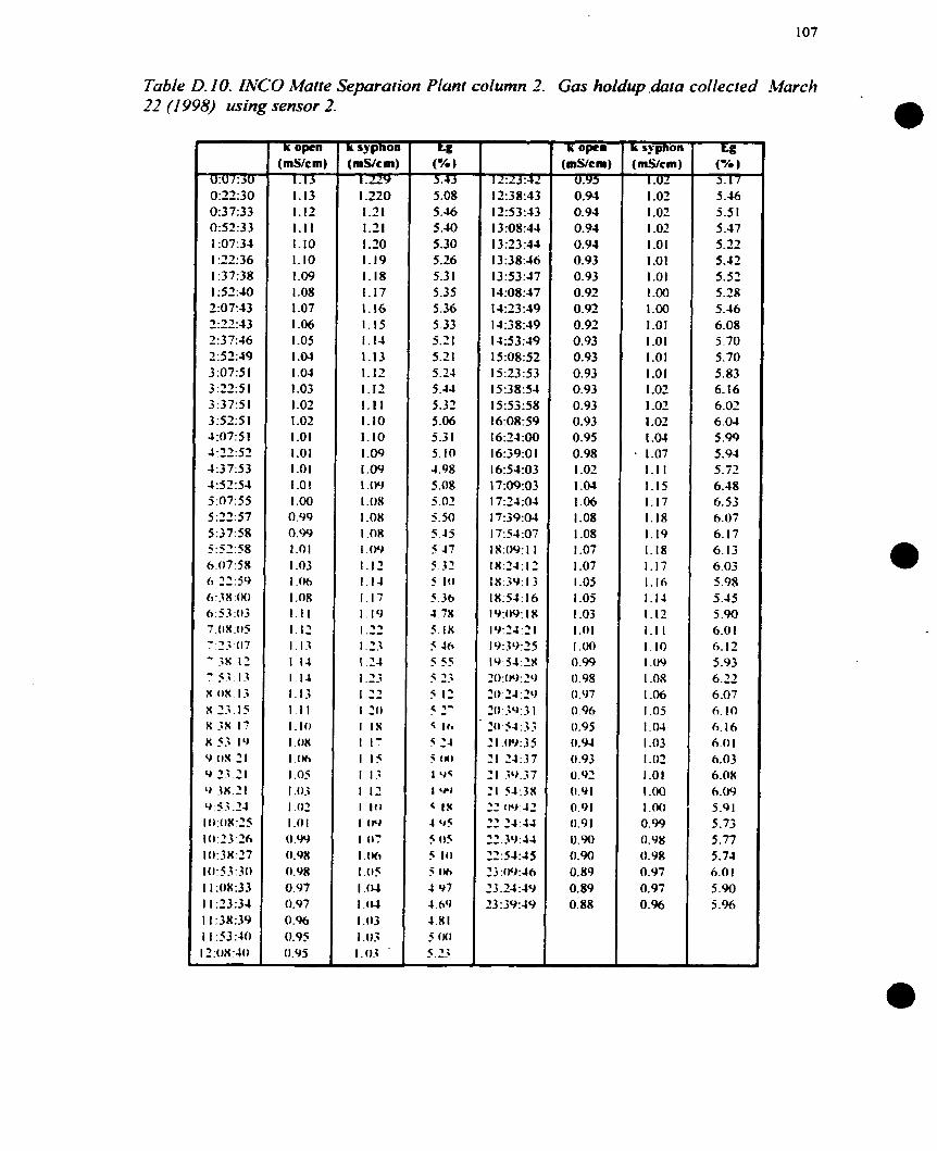
1 O7
Table D. 1 0. INCO Matte Separarion Plant column 2. Gus holdup .dam collected Marck
(mS/cm)
1.220 1.2 1 1.21 1-20 1.19 1.18 1.17 1.16 1.15 1.14 1.13 1.12 1.12 1.1 1 1.10 1.10 1.09 1.09 1-04 1 -08 1 .O8 I .on I .O9
1.12 1.14 1.17 1.19 1.12 1 .23 l 24 1.3 1 1' I Zr) 1 1% 1 1 - I 15 11; 1 12 I Ili I trr I tif 1 .im I .oc I .(cl I .CU 1-03 I .o; 1.03

Table D. I I . IXCO Matte Separarion Phnr column 2. Gas hoZdup data collected Mrch

Table D. I 2 INCO Matte Separation P la~t column 2. Gar holdup data collected March 24 (1 998) using sensor 2.

110
Table D. 13. INCO Marie Separafion Plant coiumn 2. Gus hofdup dala collecred March

1 1 1
Table D. 14. INCO Matte Separation PIant column 2. Gas holdup data collected March 26 (1 998) using sensor 2.
w sy pnon (mS/cm)
1.14
I . I1 1.15 1-17 1-19 1-21 1.23 1.24 l -24 1 .23 1.23 1-22 1.21 1-20 1.20 1.19 1.19 1.18 1.18 1.18 1.18 1.18 1.18 1.18 1-20 1.22 1-24 1-25 1.27 1.28 1-29 1.29 1.30 1.29 1-29 1-28 1.27 1.26 1-24 1-24 1-23 1.24 1.26 1.27 1 .26 1-25

112
Table D. 15. INCO Mutte Separation Plant column 2. Gas holdup data colfected lMarch 27 (1 998) using sensor 2.
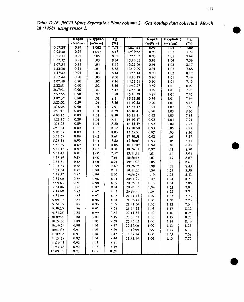
113
Table D. 16. INCO Marte Separaiion Plant column 2. Gus holdup.daro colleetrd Match ,
w =Y Pnom (mSlcm)
1.057 I .O5 1 .O5 1.04 1 .O4 1-03 1 .O3 1 .O2 1.02 1 .O2 1 .O2 1.02 1.01 1 .O1 1.01 1.01 1 .O 1 1.01 1.02 1 .O2 1.02 1 .O 1 I .O 1 1-01
1 . ( X I
1 .in) 1 .(MI 0.w 0.w
O . ' N
0 9%
O trx
O C r
O 9'
( t 'r ( 1 'Hl
0 <HI ( 1 Vf t I 'P) I ( H l
1 O'
I 0 3 1 .O3 1 .O4 1 .OM I .or I .oc 1.05
u sypnon (mYcm)
1.u5 1.05 1 .O5 1-04 1 .O3 1 .O2 1 .O2 1.01 1.01 1.01 1.01 1.01 1.01 1 .O t 1 .O2 1 .O3 1 .O3
- 1-04 1 .Cu 1-05 1 .O5 1 .OS 1 .O5 1 .O8 1. 1 1 1.11 1.17 1-20 1.22 1.24 1 . 3 1 -24 1.14 1 .2j 1.22 1-21 1-20 1.18 1.17 1.16 1.15 1-14 1.13 1.13 1.13 1.13

114
Table D. 1 7. M O Mutte Separarion Plant column 2. Gus holdup data collecrrd Jfarch 29 11 998) using sensor 2.
l q x z (mSJcm) l T T
1.120 1.1 1 1.10 1.09 1 .O8 1 .O8 I .O7 1 .O6 1 .O5 1 .O5 1 .O5 I .04 I .M 1 .O3 1 .O2 I .O 1 l .(K) 0 . w O w O V*
o vn O v- O 'J-
O km 0 Wb
( 1 '45
O V C
il W r
O '4-
Il us ( I 'CL1
1 I I ,
1 JI
1 11 l 11:
1 1 1 :
l f l :
1 1 1 :
I ( 1 I 1 ( i l
O 'P l
I I Y'
( J 'Ur
(1 'Wr
Il '45 O '14
II '1C
4 1 '15

Table D. 18. INCO Maffe Separaiion Plant column 2. Gus holdup data collecied March
OP="
(mS1cm) 1-01 1 .O8 1 .O8 1.09 1 .O9 1.1 1 1.12 1.17 1.21 1.29 1.35 l,39 r .43 I .J7 I .J9 1 .SZ 1.54 I .F6 1.57 I 57 1 .vl 1 5 5 I 5 ; 1 1'4 1 4 5 l J J
1 l ( 1
1 :9 I :K 1 :- 1 ;z
1 :! 1 :;
l :: I ; 1
i ; I 1 :4 i
1 I l -

II6
Table D.19.a. INCO Matte Separalion Plant column 3. Gas holdup data colfectrd

Table D. 19.6. Continuation fiom Table D. 19.a.
=Fi== (mS1cm) 1.23
1-22 1-22 1.21 1-21 I.20 1-20 1.20 1.19 1.18 1.18 1.17 1.17 1.16 1.16 1-15 1-15 1-15 1.15 1.15 1.16 1.15 1.16 1-16 1-10 1.16 I . l h 1.16 1.10 I . l a 1.16 1.16 1.16 I Ih
1 Ifr
1 Itt I I t r
1 It* 1 l t l
I 1t.
I t r * 1 lh
1 . I t l 1 Ir, 1.16 1.16 1.16 1.16 1.Ib

Table D. 19. c. Continuation fiom Table D. 19.6.

Table D. 20. Measured grades for INCO test.
Ti- m 10.56 11.10 13.82 13-97 13-93 12.2 1 10.88 10.15 -
Tuhfe D. .? I . Grude d u e s rrsv J to estikiu~re rhe weighrsfor the mass balunce u~trsrrnmrs
I I 1 1 I I I I I Average I 1 8.06 0.14 1 0.42 174.17 1 3.511 1 0.06 I 0.30 1 b4.33 1 I I
7262 1 0.22 1 0 . c I 1 I I I I 1 1 I 1 1 I

Table 0.23. Recovery and @pical deviation d u e s for NCO test.
Tuhfr D.24. Data on Airfloii. rate. Ia*el ( f i d depth) and solidpercent for /.!*CO lesr.

Table D.2j.a. Dafafiom two sensors ut di#ierent deplhs inside column 3. Sensor I al 4- rneïer deprh and sensor 2 at 7-meter depth.
Time
8:07:28 8: I N 9 8: 1729 8 2 2 3 0 8:27:30 8:32:30 8:37:30 8:42:30 8:47:30 8:52:31 8:57:3 1 9:O2:3 1 9:07:32 9: l2:32 9: 17:32 9:22:32 9:27:33 9 3 2 3 3 9:37:33 9:41:33 9:47:33 9 5 1 3 3 9:57:34 10:02:34 1 O : O i : j j
10: 1 3 5 I O : 1 7:3C 10:22:3t> 10.27;jh i ri:32:36 10.3?33 I o J : 3 7 lo:J7:37 10:52:37 10:57: 37 1 1 :O2127 1 1 :0?:37 I I:I2:3X 1 1: 17:3X
,
k syphon (mS1cm)
1 S U 1.50 1-50 1.50 1-50 1.50 1.50 1.50 1.50 1.50 1 .JO l .49 1-49 1.49 I .4U 1.49 1 .JX I Jn 1 4% 14% 1 J' 1 J' I J' 1 4- I Ji-
l Jti
1 4h 1 10
I 4fr
1 l f 1
I JI.
f 1'
I If.
l 1 8 %
- 1 0.
l W .
l I r .
1 U.
l a*.
I J -
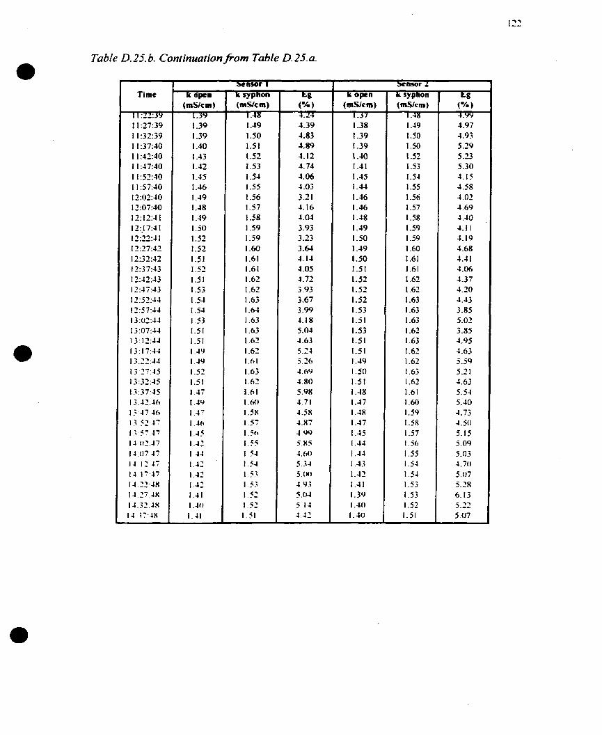
Table 0.25. b. Continuation fiom Table D. 25. a.
k syphon (mSlcm)
1.48 1-49 1.50 1.51 I .5Z 1.53 1.54 1.55 1-56 1.57 1-58 1.59 1.59 1.60 1.61 1.6 1 1.62 1.62 1.63 1-64 1.63 1.63 1.62 1.61 1.61 1.63 I .hZ 1 .tl l I .HI 1 .CK 1.57 1 . i t l 1.35 1 3-1 1 ..il 1 . z ; I 3.; 1 2' 1 .SZ 1.51


Table E. l. Erperimental dam on gas holdup: gas holdup f iom pressure versus gas. hoId~ipJ;orn conduciivity. Every point is the average of 25 min of operation. (Zast 4 points correspond to jetting sparger tests). Temperature 323 K.

Table E. 2. Test conditions for BO WA TER tests
1 s t R
1 A- l 1 A-? I A-3 I A 3 1 A-5 10-1 1 8-2 1 B-3 1 B 3 1 B-5 1 C- l I C-2 I C-3 1 C-l 1 C-5
2.4-5sp 2 A-Ssp 2.4-3sp ZB-5sp ZB-lsp îB-jsp 5.4-Ssp 3.4-4sp
-;.A-4sp-b -; B-Ssp ;B-4sp
;B-lsp-b 4. l - I 4.A-2 4 .A - 3 4.A-4
(min-) 3.z 3.2 3 -2 3.1 3 -2 6.0 6.1 6.3 6.2 6.1 5.8 6.2 6.2 6.1 6.2 3.3 3.4 3 -5 6.0 6.2 6.6 6.9 7.2 6.9 7.3 7.4 7.2 6.0 6.1 6.1 6.7

Table E. 3. Flotat ion eficiency and brighrness gain for BO WA TER tests.
. 1 est e
1A-1 1 A-2 1 A-3 I A 4 I A-5 1 5 1 I B-2 I B-3 I B-l I f3-5 fC-l I C-2 I C-3 I C-l 1 C-5
ZA-SSP ZA-lsp ?A-3sp ZB-5sp ZB-lsp 2 B-3 sp 3 t l - 5 ~ ~ ;A-lsp
;A-4sp-b 3B-jsp 3 B-Jsp
3R-lsp-b
- - m teed
1075 975 934 915 12% 1225 1308 1226 1 146 1230 1187 1207 1319 1 290 101 1 98 1 1023 1255 1167 I 142 120 I 1095 1233 1100 94 5 IO43
n ) accepts - 3443
3 89 441 739 927 308 31 l 338 476 1 O7 1 32 1 348 3 72 460 1048 446 F 16 869 3 16 4;o 94 5 275 332 439 298 355 352
t tticrency ( 9 6 ) bl.7
63.8 54.7 20.9 0.0 74.8 74.6 74.2 6 1.2 6.5 73 -9 70.7 69.1 65.1 18.8 55.9 47.1 15.1 74.8 63.2 17.3 77.1 w 7
t 4 4 1.
-9 O h2.5 M. 2
t eed 45.95
36.06 47.43 48.02 47.96 42.95 42.7 1 42-48 43.60 43.45 43.50 43.35 42.94 43 -77 42.95 44.20 46.03 46.53 43-16 44.35 45.45 43.4 I 45.4 1 44.87 45.73 47.39 46.23
accepts 3 1-06 56.07 55.85 50.92 47.62 -56.2 1 56.5 1 55.9 1 52.97 46.25 56.03 55.90 55.35 54 -27 45.56 52.67 52.23 48.29 57.40 55.13 48.19 58.42 57.36 55.58 58.31 57.00 56.66
C a m - 11.1 I 10.0 1 8.42 2.90 0.00 13.26 13.80 13.43 9.37 2.80 12-53 12.55 12.4 1 10.50 2.6 1 8.47 6.20 1.76
IJ.24 10.79 2.74 15.0 1 1 1.95 1 O.? 1 12-58 9.6 1
10.4;

Table E. 4 Test condition for test dB-jsp Hf = 100 cm: 5 spargers: r = 6 min..

Table E.5 Test condition for test ZB-4sp Hf = 100 cm: 4 spargers: r = 6 rnin..

Table E.6. Test condition for test 223-3sp Hf = 100 cm: 3 spargers; r = 6 min..
tlP (*A)
S.P 9.2 9.9 9.7 8.4 9.2 9.5 8.7 9.4 9.9 9.4 8.7 9 2 9.6 8.3 8.8 9.7 9.5 9.0 9.4 8 -4 8.3 8.9 9.1 8.5 9.1 9.;
8.X n.7 n-3 'J. I X.7 Y . -: 9. I 8.7 n . 9 - - I I
x 'J
Y' 0 I
O
n 5 X X x 5 n 2

Table E. 7. Test condition for test 2A-jsp H/ = 100 cm: 5 spargers: r = 3 min..

Table E.8. Test condition for tesr ?A-4sp 4 = 100 cm: 4 spargers: -r = 3 min..

Table E. 9. Test condition for test ZA-3sp Hf = 100 cm: 3 spurgers: r = 3 min..
Ym (cmHZ01
Laa.Y 288.7 289.0 288.6 288.9 289.7 289.0 290.0 289.5 289.8 288.3 289.8 289.4 289.0 289.5 290.3 290.0 289.2 289.5 289.8 290.5 291.1 289.8 290.6 289.7 290.3 189.7 190.R 289.5 289.5 29 l .O
289.5 290.2 2nv.x ?XX h
2x9 4 2VO.h 2n9 - '90 x 'X0.5 29 1 .ll .xu K 291 O
190.' 'XV ' -

Table E. IO. Bubble size. bubble surface aareaflux and collection zone rate constant . esfirnafed for BOWATER tesrs. Bubble sizes over 0.2 cm are invalid
lcsl s
I A-T I A-2 I A-3 I A 4 I A-5 I B-I I B-2 1 5 3 1 B4 1 B-5 1C-1 1 C-2 IC-; ICA I C-5
2 A-Ssp A 4 s p Z A-3sp 2 6-5 sp 2BAsp 25-isp .;A-Ssp .:A-lsp
;A-!spb :R-?sp 7n4sp
:B4\pb J A - I 4A-2 JA-; 4 A-!
JI3 (JU h ( a n i s )
, i -.- 1.77 1 36 0.86 O66 2.79 '3.4 1.86 1 37 090 2 70 2.29 181 1 32 O 89 2 JI 2 35 2.32 2.34 2 22 2.31 1 76 I f 5 . 9.7
l -3' l -73
1 68 2 32 7 94 1 40 1 08